Technical note: A view from space on global flux towers by MODIS and Landsat: the FluxnetEO data set

The eddy-covariance technique measures carbon, water, and energy fluxes between the land surface and the atmosphere at hundreds of sites globally. Collections of standardised and homogenised flux estimates such as the LaThuile, Fluxnet2015, National Ecological Observatory Network (NEON), Integrated Carbon Observation System (ICOS), AsiaFlux, AmeriFlux, and Terrestrial Ecosystem Research Network (TERN)/OzFlux data sets are invaluable to study land surface processes and vegetation functioning at the ecosystem scale. Space-borne measurements give complementary information on the state of the land surface in the surroundings of the towers. They aid the interpretation of the fluxes and support the benchmarking of terrestrial biosphere models. However, insufficient quality and frequent and/or long gaps are recurrent problems in applying the remotely sensed data and may considerably affect the scientific conclusions. Here, we describe a standardised procedure to extract, quality filter, and gap-fill Earth observation data from the MODIS instruments and the Landsat satellites. The methods consistently process surface reflectance in individual spectral bands, derived vegetation indices, and land surface temperature. A geometrical correction estimates the magnitude of land surface temperature as if seen from nadir or 40^∘ off-nadir. Finally, we offer the community living data sets of pre-processed Earth observation data, where version 1.0 features the MCD43A4/A2 and MxD11A1 MODIS products and Landsat Collection 1 Tier 1 and Tier 2 products in a radius of 2 km around 338 flux sites. The data sets we provide can widely facilitate the integration of activities in the eddy-covariance, remote sensing, and modelling fields.

1 Introduction

The installation and maintenance of instrumental infrastructure at eddy-covariance (EC) sites worldwide require considerable financial and logistical efforts and labour force. The precious data sets of land–atmosphere fluxes, biometeorological data, and environmental conditions allow fundamental insights into ecosystem functioning (Baldocchi, 2008; Baldocchi et al., 2018; Baldocchi, 2020; Besnard et al., 2018; Migliavacca et al., 2021; Nelson et al., 2020). A significant achievement is the central processing, quality control, and open standardised distribution of a large number of the available observational records in data collections such as LaThuile, Fluxnet2015, and ABCflux (amongst others, Papale et al., 2006; Baldocchi, 2008; Pastorello et al., 2020; Virkkala et al., 2022; Papale, 2020) to which many site teams contribute.

Complementary information from satellites or digital cameras (phenocams,  Wingate et al., 2015) aids and refines studies of local land–atmosphere interactions as they relate to ecosystem structure, phenology, and functioning and the state of the land surface (e.g. Migliavacca et al., 2015; Bao et al., 2022). Earth observation (EO) data for varying regional sizes around the sites can represent the actual area that contributes to the flux measurements – partly even more accurately than similar ground-based measurements can (Gamon, 2015) – provided sufficiently high spatial resolution and temporal overlap with the site-level records. Next to local studies, the combination of flux and satellite observations is also a basic ingredient for upscaling exercises of the in situ fluxes to larger areas or even the globe (Ueyama et al., 2013; Tramontana et al., 2016; Jung et al., 2019, 2020; Joiner et al., 2018; Reitz et al., 2021; Virkkala et al., 2021; Zeng et al., 2020).

Independent of the nature of the scientific application, the quality control and gap structure of both the EC and the EO data are the groundwork of each analysis. Different criteria help to identify problematic data points with differing levels of strictness depending on the given application. Moffat et al. (2007) and Falge et al. (2001) describe techniques to fill gaps due to missing data points in the EC data. The literature also offers a diverse set of methods to gap-fill EO data that include spatial, temporal, cross-sensor, and cross-variable approaches (to name a few, Wang et al., 2012; van Buttlar et al., 2014; Weiss et al., 2014; Verger et al., 2011, 2013; Kandasamy et al., 2013; Moreno et al., 2014; Moreno-Martínez et al., 2020; Yan and Roy, 2018; Ghafarian Malamiri et al., 2018; Li et al., 2018; Dumitrescu et al., 2020; Bessenbacher et al., 2021). The pre-processing steps are laborious, and they are key to the results and interpretation of the analyses.

We propose a set of systematic pre-processing steps for key land surface indicators from EO data: sub-setting global EO data for an area around an EC site; systematic control for good-quality retrievals as well as cloud, snow, and water effects; and estimating missing data points in a flexible and ecologically meaningful way. For both the quality control and the gap filling, the approaches aim to be generalisable across all sites without accounting for specific local conditions, yet flexible enough to accurately reproduce phenological behaviour and characteristic features such as disturbances or fast transitions in managed ecosystems. The procedure shall be as simple as possible, computationally efficient, and not resort to additional data sources to facilitate a potential application to EO data at the global scale.

We apply the proposed processing steps to official data products from the Moderate Resolution Imaging Spectroradiometer (MODIS) instruments and the sensors on board the Landsat satellites. Both MODIS and Landsat have extensive observational coverage with a high temporal overlap with most freely available EC records. Landsat measurements are of particular interest because they resolve small spatial details in pixels of 30 m size, but at the cost of missing out on short temporal features. The opposite is true for MODIS data products, which partly average over heterogeneous areas in spatially comparatively coarse pixels of several hundred metres. However, MODIS offers daily, partly even sub-daily, temporal resolution. We process EO data sets of surface reflectance, vegetation indices, and land surface temperature (LST) for a limited area around a given flux site.

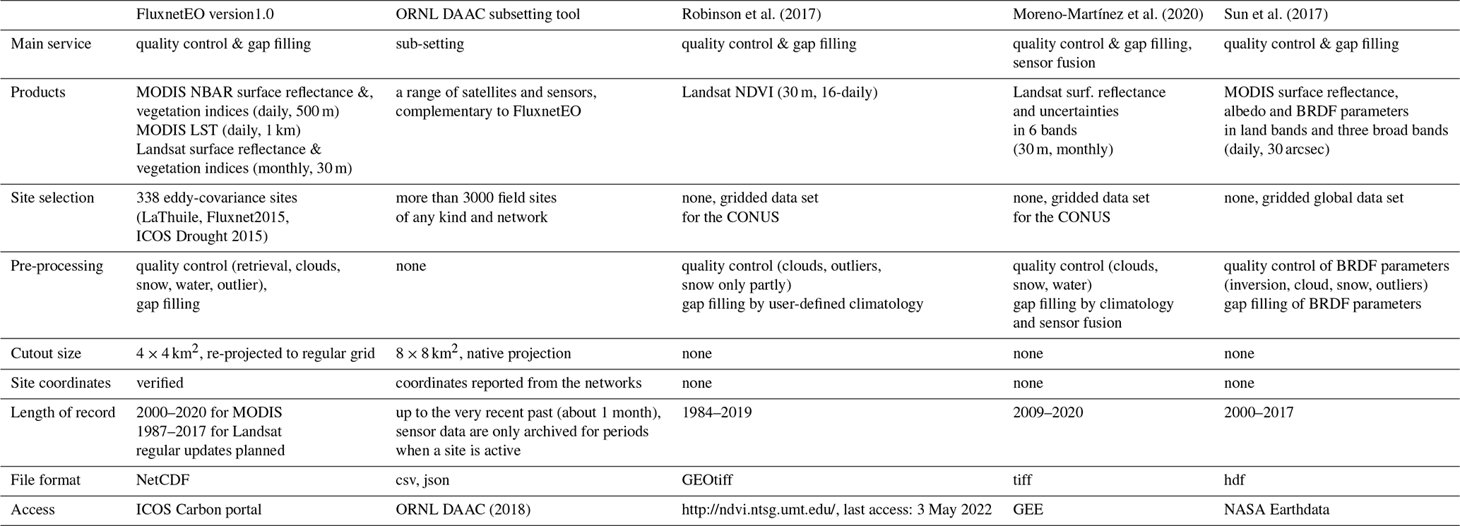
As missing data points in EO data are a ubiquitous problem, a number of related initiatives also provide access to EO data that underwent certain pre-processing. For example, Robinson et al. (2017) offer 30 m Landsat NDVI for all pixels in the CONUS every 16 d between 1984–2019. They removed cloud effects and filled gaps with climatological averages. Moreno-Martínez et al. (2020) controlled Landsat and MODIS surface reflectance for cloud, snow, and water effects and fused them to a gap-free and smoothed product. It covers surface reflectance and its uncertainty in six Landsat spectral bands at monthly, 30 m resolution for the CONUS and the years 2009–2020. An example product for gap-free MODIS surface reflectance (as well as albedo and BRDF parameters) at approximately 1 km resolution is the MCD43GF product (Sun et al., 2017). In this case, the time series of the parameters of the bidirectional reflectance distribution function are temporally and spatially gap-filled for days and pixels with bad inversion quality or cloud and snow influence, and from those gap-free model parameters a global gap-free product of surface reflectance is provided for the MODIS land bands and three broad spectral bands. Finally, a sub-setting tool (ORNL DAAC, 2018) facilitates access to a range of global EO data sets at a large selection of eddy-covariance sites.

FluxnetEO is unique in proposing the completion of all pre-processing steps necessary for scientific analysis at site level, hence resulting in an analysis-ready data set. The products in version 1.0 of the data cover the period 1984–2017 and 2000–2020 for Landsat and MODIS, respectively, and are freely available by the services of the ICOS Carbon Portal (see data availability statement; Walther et al., 2021a, b). Each data set has a complementary data layer with additional flags to inform the user whether data points correspond to actual good-quality observations according to the proposed criteria and, if not, how they have been estimated in different gap-filling steps. FluxnetEO provides a ready-to-use data set, which, however, means limited flexibility for the users to make their own decisions on the pre-processing steps. For example, they depend on the site selection made by the authors (see Table E1 for the site selection in version 1.0) and their decision to cover an area within a radius of 2 km around a site. Conversely, the ORNL DAAC (2018) offers larger cutout radii of 4 km around a considerably larger collection of sites than FluxnetEO and from a complementary selection of global EO products. But users will need to invest considerable work in quality control and gap filling. Regarding available quality-controlled and gap-free large-scale or even global gridded EO data (Moreno-Martínez et al., 2020; Robinson et al., 2017; Sun et al., 2017), the user needs to find ways to access these data sets at site level (while Moreno-Martínez et al., 2020, is available on Google Earth Engine (GEE), Sun et al., 2017, is not, and Robinson et al., 2017, needs shape files) and needs to understand whether the applied quality filters match the needs of their application.

To allow potential users to make an informed decision on the product which suits their application best, we describe details about data inputs in FluxnetEO in Sect. 2.2, explain the quality control and gap-filling approaches in Sect. 3, illustrate examples, and benchmark the products against a selection of independent products and approaches in Sect. 4. Table 2 and the data availability section provide detailed information on the resulting products, while Table A1 summarises and compares the main characteristics of the selected studies and services mentioned above (Robinson et al., 2017; Sun et al., 2017; Moreno-Martínez et al., 2020; ORNL DAAC, 2018) and the one in this contribution. We expect FluxnetEO to be a living data set with regular updates regarding the site selection, the temporal coverage, the release of new Landsat/MODIS collections and processing improvements based on user feedback. Potential users are therefore advised to refer to the ICOS Carbon Portal for the latest product version and site availability information (Walther et al., 2021a, b).

2 Data

2.1 Eddy-covariance sites

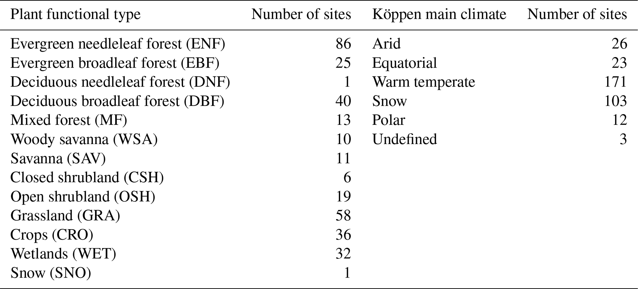
For the current version 1.0 of the product we select the 338 sites from the LaThuile, Fluxnet2015 (Pastorello et al., 2020), and ICOS Drought 2018 Initiative (Drought 2018 Team and ICOS Ecosystem Thematic Centre, 2020) flux data releases. Site coordinates given in different sources (AmeriFlux, AsiaFlux, Europe-Fluxdata, Fluxdata.org, and a previously compiled in-house Fluxnet site location list) may differ. In that case, the coordinates with the highest precision were selected. In case the coordinates differed by more than 0.001^∘ for a given site, a manual check in Google Earth identified the correct or most probable location of the site. The final set of 338 sites for which we process the MODIS and Landsat EO data in product version 1.0 is listed in Table E1. Forests and grasslands are best represented among the 338 sites. The collection includes fewer sites from savannas and shrublands and only one site from a deciduous needleleaf forest (Table 1).

Table 1 Representation of different plant functional types and Köppen climate classes across the 338 sites in the FluxnetEO v1.0 collection.

2.2 MODIS and Landsat

The MCD43A4 product combines Aqua and Terra observations and provides estimates of surface reflectance in the MODIS bands 1–7 (Schaaf and Wang, 2015b). Time series represent observations modelled at nadir view at a resolution of 16 d and 500 m spatial pixels. For the quality control of MCD43A4, a complementary product, MCD43A2, contains band-specific information on the quality of the inversion of the bidirectional reflectance distribution function as well as snow cover, platform information, and land–water coverage in the scene (Schaaf and Wang, 2015a).

The MODIS MOD11A1 (Terra, starting in 2000) and MYD11A1 (Aqua, starting in 2002) products (hereafter jointly referred to as MxD11A1, Wan et al., 2015a, b) provide daily LST and emissivity estimates aligned with quality and view angle information at 1 km spatial pixel sizes. The LST values represent instantaneous values and are selected based on viewing zenith angle and LST values (MOD11A1 user guide, https://lpdaac.usgs.gov/documents/118/MOD11_User_Guide_V6.pdf, last access: 3 May 2022). Four LST data streams are available: TERRA_day with observations around 10:30 local time, AQUA_day with observations around 13:30 local time, TERRA_night around 22:30 local time and AQUA_night around 01:30 local time. For each of them, observation times vary between overpasses by about ± 1.5 h.

Observation geometries need special attention as the MODIS instruments measure in a wide swath to obtain high temporal coverage. They scan across their track from right to left with view zenith angles up to 65^∘ from nadir. The wide range of viewing geometries leads to different fractions of surface types seen from one overpass to the next for a given site. In addition, vegetation structure and topography, together with the position of the sun relative to the sensors, cause variable shadowing effects. The reflectance product (MODIS MCD43A4, Schaaf and Wang, 2015b) partly accounts for these anisotropy effects and simulates a nadir view. In order to partly account for variability in the observed LST that is related to changing observation geometry (Rasmussen et al., 2011; Guillevic et al., 2013; Ermida et al., 2014), a correction approach developed by Ermida et al. (2018) estimates an LST offset as if the instrument were measuring from directly above a site. For some applications, an oblique view might be favourable over a nadir constellation, for example to enhance the contribution of vegetation canopy to the LST estimate and minimise fractions of soil or understorey. In addition, we provide LST corrected to a viewing zenith angle of 40^∘.

Reflectance-based Landsat time series comprise the entire multi-temporal collection 1 of the Landsat 4, 5, 7, and 8 archives (https://landsat.gsfc.nasa.gov/data, last access: 3 May 2022) covering the period 1984–2017 at 30 m spatial pixel size. The seven spectral bands of the Landsat product were collected: blue, green, red, near infrared (NIR), shortwave infrared 1 and 2 (SWIR1, SWIR2), and thermal infrared (TIR) (https://landsat.usgs.gov/what-are-band-designations-landsat-satellites, last access: 3 May 2022). Landsat data have been pre-processed using the Landsat Ecosystem Disturbance Adaptive Processing System (LEDAPS, Schmidt et al., 2013) and the Landsat Surface Reflectance Code (LaSRC, https://landsat.usgs.gov/landsat-surface-reflectance-data-products, last access: 3 May 2022) for atmospheric correction. The pixelQA layer contains information related to clouds, cloud shadows, snow, and water and is useful for the quality control of the Landsat data (Zhu and Woodcock, 2012; Zhu et al., 2015). In contrast to MODIS, the Landsat sensors acquire images at much smaller view angles around 7.5^∘ from nadir. Ground control points and a digital elevation model help to correct for small directional effects related to terrain structure and viewing angles (Wulder et al., 2019). Corrections for the small but significant differences between the spectral characteristics of Landsat ETM+ and OLI (Roy et al., 2016) are not applied.

The services by GEE provided cutouts of the above-mentioned products at the EC sites. Independently of the product and its spatial resolution, the cutout area was limited to a maximum distance of 2 km between a given tower and the centre of a given satellite pixel. No single cutout size will fit the flux footprint extents of all sites (Chu et al., 2021). The decision for a radius of 2 km in product version 1.0 compromises reasonable data set sizes and the inclusion of the high-temporal-resolution flux footprints for the majority of sites. Downloading the EO data in tiff format avoided nontransparent re-projection of the data from sinusoidal to regular grid by GEE, which would have been problematic for the quality flags in the MCD43A2 and MxD11A1 products. The Landsat data were already provided in regular grid by GEE.

3 Methods

We describe here the overall concept and rationale of the quality filter and the gap filling, but we report all technical details in Appendix A.

3.1 Processing steps of reflectance-based indicators

The processing steps for reflectance-based land surface variables can be summarised by the following steps:

1. quality control for effects of snow, water, bad inversion per spectral band, and individual pixel in a cutout (henceforth subpixel) using the MODIS/Landsat quality flags;

2. optionally compute vegetation index per subpixel, or use the raw spectral bands;

3. optionally spatially aggregate over a selection of subpixels in the cutout to obtain one time series per site, or decide to process all subpixels individually;

4. remove values of an index outside its defined ranges and apply an additional outlier filter;

5. gap filling.

3.1.1 Quality control and computation of spectral indices

Quality control of the MODIS reflectance-based vegetation indices focused on three aspects: good inversion quality of the bidirectional reflectance distribution function as indicated by the BRDF_Albedo_Band_Quality_Bandx flags in the MCD43A2 product, snow-free conditions according to the Snow_BRDF_Albedo flag, and the omission of reflectance values that are affected by the presence of water in the field of view using the BRDF_Albedo_LandWaterType flag. For the selected data samples which passed those criteria, we computed a large set of spectral vegetation indices (Table 2). An additional check removed possible values of the vegetation indices outside their defined ranges. Some of the time series contained obvious outlier values. We employed an empirical filter which largely removed those samples which had a particularly large difference to the median of their surrounding values in a temporal window (Papale et al., 2006, technical details on all filters in Appendix A).

In the Landsat data, the flag pixel_qa provided quality attributes (CFMask, Foga et al., 2017) and removed pixels that contained snow/ice, water, cloud, and/or cloud shadow using a binary flag of presence. Similar to the MODIS product, we computed a series of spectral vegetation indices (Table 2) using the good-quality observations and removed possible values of the indices outside their defined ranges. A slightly modified filter removed possible outlier values also for the Landsat data (see details in Appendix A.).

3.1.2 Gap filling

In the literature several gap-filling and smoothing approaches are available which work in one or more dimensions (e.g. Wang et al., 2012; Kandasamy et al., 2013; van Buttlar et al., 2014; Weiss et al., 2014; Yan and Roy, 2018; Zhang et al., 2021) or use fusion methods between sensors (Verger et al., 2011; Moreno-Martínez et al., 2020). They differ in their levels of sophistication and computational efforts. One of our requirements for the gap-filling approach was that it employs exclusively temporal operations and does not use additional data sources. It is hence very generalisable and allows the gap filling to be generally applicable to a single time series per site, several subpixels in a cutout around a site, and global EO data. A number of possible applications will require the analysis of actual observations, and consequently approaches that fit smooth functions to available good-quality data (e.g. Jonsson and Eklundh, 2002; Gonsamo et al., 2013) to represent a gap-free time series are not suitable. Therefore, the idea was to retain the good-quality data and make as realistic of estimates as possible for the gaps between them. The following recipe describes the steps to estimate missing data points conceptually; all technical details we report in Appendix A. Unless stated otherwise, for each gap-filling step, the values filled in previous steps guide the current and subsequent gap-filling steps together with the good-quality observations.

1. Fill short non-snow-related gaps (≤ 5 d or ≤ 1 month for MODIS and Landsat, respectively) with a median across valid values in moving windows of 16 d (3 months for Landsat). The moving median only fills gaps; it does not change/smooth valid data points.

2. Fill snow-related gaps with a constant baseline value which is identified as the average of valid data points adjacent to snow-covered periods, i.e. immediately before snowfall or after snowmelt (after  Beck et al., 2007, but see details in Appendix A). Consider all times with a snow flag larger than 0.1 or missing snow information as snow covered. The latter periods are included as the snow flag appears to systematically miss snow periods in higher latitudes in the beginning of the winter. Still, frequent gaps with missing snow information also occur during the growing season. In order to avoid wrong filling with a constant value during the growing season, this gap-fill step is not applied when the probability of snow cover is low, i.e. when the average seasonal cycle indicates typically snow-free conditions at a given time of the year, or when typically no snow occurs at all at a given site.

3. Subsequently, another moving median in windows of 40 d (4 months for Landsat) fills gaps shorter than 65 d (2 months for Landsat).

4. Linearly regress the time series on its own median seasonal cycle (MSC). Compute a re-scaled MSC with the obtained regression parameters and use it to fill longer gaps. Execute the regression and re-scaling in temporal moving windows as this guarantees more flexibility to correctly represent inter-annual variations in the time series and even partly accounts for changes in the shape of the seasonal cycle due to disturbances. It is, however, not suited to fill regularly recurring gaps at a certain time of the year, e.g. during rain seasons (Verger et al., 2013).

5. Fill the remaining gaps by piecewise cubic polynomial interpolation. Time series with fewer than 300 valid data (12 months for Landsat) points in the whole record after application of all the previous gap-filling steps will not be meaningful for analysis but are still filled by nearest-neighbour interpolation.

6. Temporal operations cannot meaningfully fill gaps at the beginning and at the end of the record. Therefore the first (last) valid data points are repeatedly appended at the beginning (end) of the record.

The described processing steps are generalisable across a range of spectral vegetation indices and can reliably fill missing data points across sites globally (see examples in Sect. 4). However, a number of sites have extremely low data availability after quality checks, and the gaps in their time series are challenging to temporally interpolate in a meaningful way. This can lead to problematic gap-filled data points with questionable reliability and realism. Examples are tropical sites and/or sites with a pronounced wet season with permanent cloud cover. The same generally applies for MODIS in the years 2000–2002 when observations stem mainly from the Terra satellite, and therefore data availability is comparatively low. For Landsat, the number of available scenes is relatively heterogeneous across the globe (https://www.usgs.gov/media/images/cumulative-number-scenes-landsat-archive, last access: 3 May 2022), with some regions having very good coverage (e.g. North America) while other regions are observed less frequently (e.g. Russia and Africa). Such differences in the availability of good-quality data between sites strongly affect the quality of the gap filling at the site level. In addition, FluxnetEO provides for each data layer a gap-fill flag, consisting of a range of integer values to identify original good-quality data (flag = 0) from gap-filled estimates (flags = 1…n) where information is provided in which gap-filling step a certain data sample has been imputed. This allows users to explore individual sites and use (parts of) the gap-filled data or resort to only using the high-quality original data points.

3.2 Preprocessing of MODIS land surface temperature

The processing of the LST follows this order:

1. outlier filter for each LST data stream and check that any daytime LST is higher than any nighttime LST per subpixel and day

2. optionally apply a geometrical correction per subpixel

3. optionally aggregate over a selection of subpixels in the cutout per time step and LST data stream

4. gap-fill the aggregated time series or each subpixel for all four MODIS LSTs simultaneously.

3.2.1 Quality checks

The quality control of the MODIS LST focused on removing outlier values. Negative outlier values in LST might represent residual cloud contamination, whereas unusually high values might originate from undetected saturation in the level 1 data. We found that the flags provided in the MxD11A1 products are insufficient to achieve this. Instead, empirical quality checks followed the procedure for the MODIS reflectances; i.e. they discarded data points that deviated strongly from the median of their surrounding values in temporal windows of 30 d (Papale et al., 2006). An additional sanity check eliminated any daytime LST lower than the minimum of Aqua and Terra nighttime LST for a given day.

3.2.2 Geometrical correction

For several applications, variable viewing geometries as inherent in the MODIS LST observations are not desirable. A geometrical correction approach developed by Ermida et al. (2018) accounted for directionality in LST retrievals due to vegetation structure and topographical effects. A parametric model estimates the magnitude of LST as if constantly observed from nadir or an angle of 40^∘ between the sensor and the zenith above a given site. Ermida et al. (2018) derived the coefficients for this geometrical model at a resolution of 0.05^∘. We followed the pragmatic approach of selecting the model coefficients for the correction from the pixel containing a given site. We acknowledge that we did not investigate to what extent the given site conditions represent the overall characteristics of the land surface in the allocated pixel. Further input to the geometrical model were the viewing azimuth angles, solar angles at the overpass time, and estimates of daily potential radiation at the top of the atmosphere. The geometrical correction was applied to each subpixel in a cutout separately.

3.2.3 Gap filling

Also for the gap filling of LST, several approaches are present in the literature (e.g. Gerber et al., 2018; Ghafarian Malamiri et al., 2018; Li et al., 2018; Dumitrescu et al., 2020). When using exclusively operations in time and no ancillary data to estimate invalid LST observations, one needs to consider the shorter autocorrelation of LST compared to the reflectance-based indicators. According to Vinnikov et al. (2008), the weather-related component of clear-sky LST has an autocorrelation of about 3 d. The following sequence of steps filled the four MODIS LST data streams (for technical details refer to Appendix B).

1. Similar to the reflectances, a first step consisted of a temporal moving median in windows of 8 d to fill gaps.

2. A second step was inspired by Li et al. (2018) and Crosson et al. (2012) and foresaw using one of the four MODIS LST time series as a “reference” to fill gaps in a second “imputed” one. We computed a MSC of the difference between the “reference” and the “imputed” MODIS LST. This average shift was linearly scaled to the actual shift in temporal windows. The scaled average shift added to the “reference” LST represented the values used to fill gaps in the “imputed” LST time series. This procedure iteratively used three of the MODIS LST data streams to fill the fourth; i.e. each one is imputed once by all three others (see details in Appendix B). This gap-fill step was only possible in cases where not all four MODIS LST observations were invalid during a given day, but extremely advantageous to preserve short synoptic variability in the gap-fill estimates.

3. In fully cloudy days without any valid LST observation, or in case a period has too few valid observations for a meaningful calibration of the linear model in the previous step, the gap-filling followed the same steps as for the reflectance-based spectral indices: in temporal windows, find a linear scaling between one LST time series and its own MSC. Use the slope and intercept parameters to compute a re-scaled MSC, which fills gaps in the time series for days of the year when the MSC is valid.

4. Interpolate the remaining gaps with cubic polynomials, or nearest neighbour in case of very low data availability (fewer than 300 valid data points in the entire time series).

5. Missing values at the beginning and the end of the record cannot be meaningfully filled by temporal methods and are therefore simply repeated.

Steps 3–5 produced very smooth and, therefore, less realistic LST estimates than steps 1–2. Also, one needs to be aware that any LST estimate in data gaps from this procedure necessarily represents an LST estimate under clear-sky conditions, which can be very different from the real LST under overcast skies (Ermida et al., 2019). This needs to be considered for a given application to prevent the effects of clear-sky bias in the LST data sets on the results. Like the vegetation indices, LST data layers have a gap-fill flag in FluxnetEO describing which data points are original and which gap-filling step filled the missing values.

3.3 Evaluation and benchmarking

3.3.1 FluxnetEO performance in comparison to a machine learning approach (missForest)

A common approach to benchmarking gap-filling methods is to artificially remove samples at positions where the true data value is known and then subject the time series to the gap-filling approach and compare the gap-filled estimates with the original values (Moreno-Martínez et al., 2020; Zhang et al., 2021; van Buttlar et al., 2014; Wang et al., 2012; Verger et al., 2011, 2013; Gerber et al., 2018). We apply this approach to FluxnetEO in artificial gaps for MODIS and Landsat variables and randomly remove 20 % and 40 % of data samples (corresponding to a low and medium gap fraction; compare Fig. 1) per site at positions with originally good quality. We remove data points from a gap-free time series; i.e. the data points which had been gap-filled before guide the gap filling in the artificial gaps. We feed the time series of the station pixel with artificial gaps into the gap-filling approaches described in Sect. 3 and quantify the gap-filling performance compared to the true values with the Nash–Sutcliffe efficiency (NSE, Nash and Sutcliffe, 1970). NSE close to 1 indicates good performance, while negative values mean worse performance than inputting the simple average into the gaps. Decidedly, the NSE refers exclusively to the data samples from the artificial gaps and not to the complete time series.

To have an independent benchmark of FluxnetEO, we compare to the performance of a versatile imputation method, missForests (Stekhoven and Bühlmann, 2011), in the same artificial gaps. MissForest is based on random forests and can handle variables of different types and dimensions. It is a multi-output machine learning method that iteratively fills gaps across variables, considering their potential non-linear dependencies. We input all MODIS (Landsat) variables per site together with the information on snow fraction and the day of year or month of year for MODIS or Landsat, respectively. Hence, per site and mission, missForest iteratively imputes all variables collectively.

3.3.2 Comparison with other gap-filled data sets: Moreno-Martínez et al. (2020)

A complementary and mandatory approach to assessing the quality and characteristics of the proposed pre-processing steps is a comparison against independent data sets and approaches (e.g. Moreno-Martínez et al., 2020; Robinson et al., 2017; Sun et al., 2017). Different spatio-temporal resolutions in the provided data sets and the fact that often mass downloads of data are necessary to evaluate them at the site level challenge this approach. However, Moreno-Martínez et al. (2020) provide their gap-filled Landsat surface reflectance at the same spatio-temporal resolution as FluxnetEO, and access and cutout at the site level via GEE are feasible. We, therefore, compare the FluxnetEO Landsat product and the Moreno-Martínez et al. (2020) surface reflectance at 86 sites in the CONUS for the years 2009–2017, which corresponds to the spatiotemporal domain in which both are available. In the comparison, we do not differentiate between original good-quality and gap-filled estimates because quality control and, therefore, gap structure differ between the products. However, unphysical reflectance values lower than 0 or larger than 1 occur, especially in winter, and were removed before the cross-consistency analysis, from both good-quality and gap-filled estimates.

4 Results and discussion

Huete et al. (2002)Tucker (1979)Camps-Valls et al. (2021)Gao (1996)Gao (1996)Gao (1996)Badgley et al. (2017)Gitelson (2004)

Table 2 Data sets presented in FluxnetEO bx refer to the spectral bands. Each data set spans the time period 2000–2020 (MODIS) and 1984–2017 (Landsat) and contains a flag describing whether a data point is good quality or whether and how it has been estimated in the gap-filling procedures.

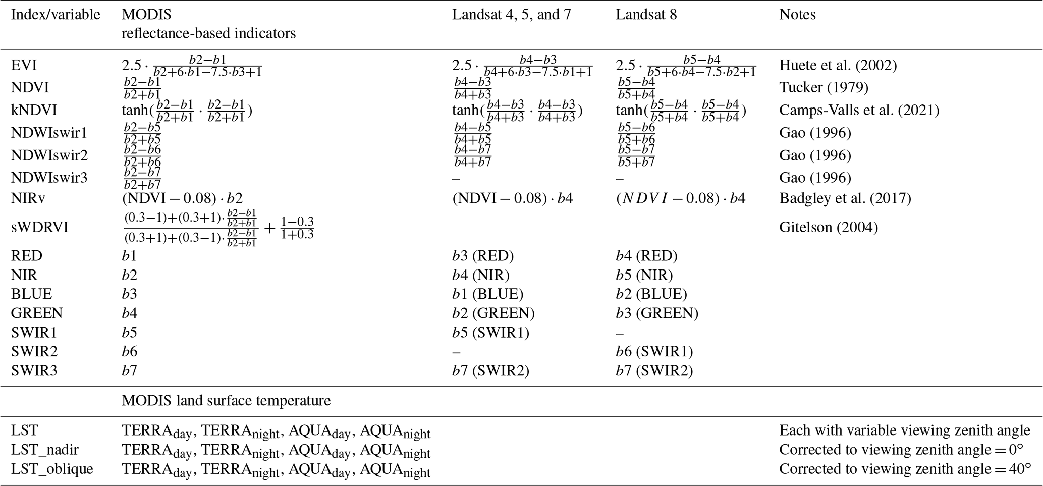
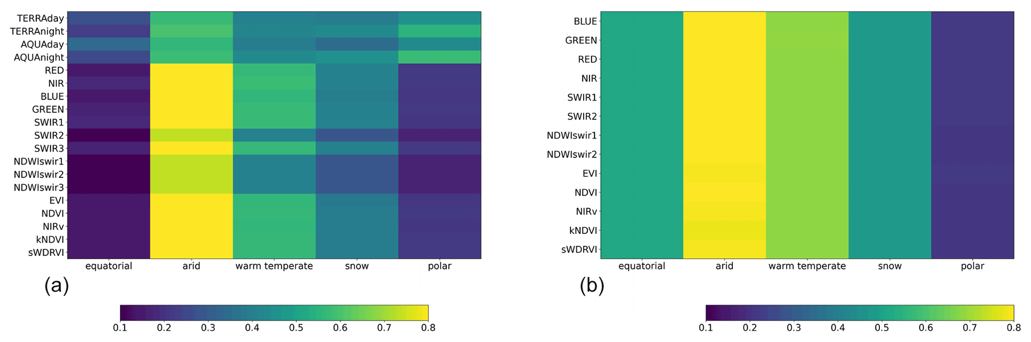
Figure 1 Fraction of good-quality data in the MODIS (a) and Landsat (b) time series. Colours represent the median data availability in tower pixels across sites grouped by Köppen climate classification. Data refer to the period 2003–2020 for MODIS (the time period when both Terra and Aqua satellites are in space) and 1990–2017 for Landsat.

4.1 Gap statistics across indices

Data availability after quality screening is highly variable between sites and depends on the data stream (Fig. 1). Large differences in the amount of good-quality data in groups of different climate regions, especially for the reflectances, mirror general atmospheric conditions in different regions. Differences between spectral bands and reflectance-based indices are very minor in both MODIS and Landsat. MODIS LST generally has fewer valid data points among the data sets than the reflectance-based indicators, and often fewer during daytime than nighttime. While the LSTs are instantaneous values, the reflectances represent averages over 16 d periods. A lower number of good-quality observations in indices that rely on band 6 relate to degraded detectors in Aqua MODIS band 6.

4.2 Temporal patterns of the gap-filled time series

We illustrate some characteristics of the time series in FluxnetEO using the pixel containing an EC station at example sites. The Austrian site Neustift (AT-Neu) was situated in a valley in the Alps and surrounded by grasslands which were typically mown three times a year (Wohlfahrt et al., 2008). According to their nature, the MODIS LST time series exhibit faster variability than the vegetation indices (Fig. 2). Midday observations (AQUA_day) partly show an LST increase after the first harvest event in a year around the 150th day of the year. The MSC of most vegetation indices clearly marks the mowing timing, although the relative magnitude varies between indices. Constant values in winter represent snow-covered times. For Landsat, the granularity of temporal patterns is clearly lower due to the monthly sampling, but the characteristic management effects are also visible here (Fig. 3).

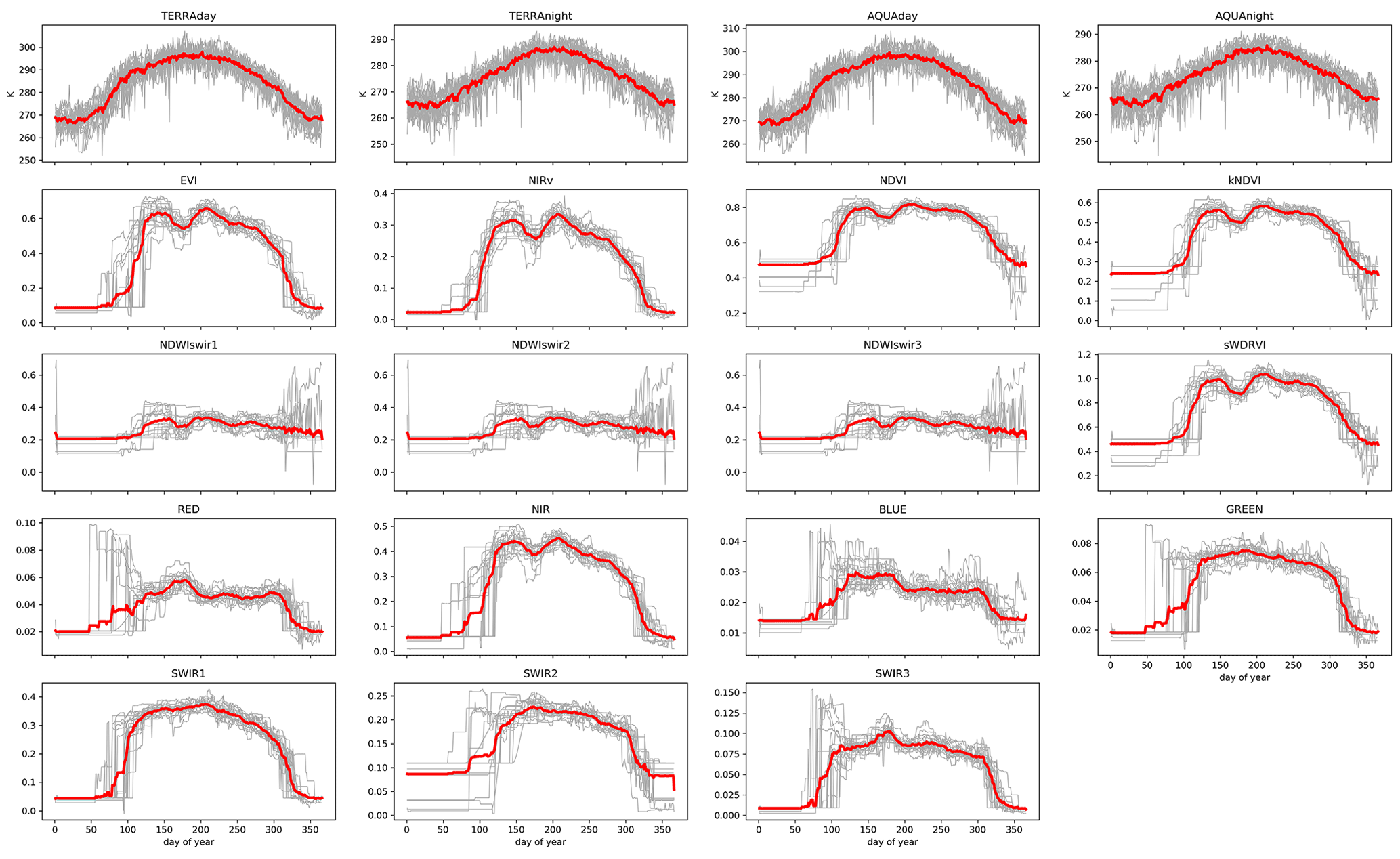
Figure 2 Median seasonal cycle (red) and individual yearly trajectories (grey) for MODIS LST (top row) and MODIS vegetation indices and surface reflectance (second to last rows) in the pixel containing the Austrian site Neustift (AT-Neu). Depending on the data set the central pixel measures 500 m or 1 km.

Figure 3 Median seasonal cycle (red) and individual yearly trajectories (grey) of the different data sets in the 30 m pixel containing the Austrian site Neustift (AT-Neu) Landsat.

Focusing on the example of the EVI, other sites illustrate a few characteristics of the gap-filling procedure in more detail (Figs. 4, 5): at the evergreen needleleaf forest site El Saler in Spain (ES-ES1) much data pass the quality control, and mostly short gaps are reliably filled, also in the absence of a very regular seasonal cycle in EVI in both MODIS and Landsat. The boreal forest site Saskatchewan (CA-SF1) illustrates the effect of a disturbance that happened in 2015 (though the site was operated only until 2006). The gap-filling procedure adapts to the modified conditions both abruptly when the disturbance happens and gradually during recovery in the following years. There is a problematic group of high MODIS EVI values during winter 2006/2007. The moving window outlier filter applied to the MODIS reflectances is by design unable to detect those outliers as they occur consecutively in a short period of time. Tharandt (DE-Tha, evergreen needleleaf forest) and Lonzée (BE-Lon, crops) are examples of the challenges that data-scarce periods bring for both Landsat and MODIS. For MODIS, estimated values in the years 2000–2002 (where only Terra was in operation) are less reliable at both sites. Landsat is particularly scarce and the gap filling unsuccessful at Tharandt in the 1980s, 1994–1995, and 2008–2012, and in Lonzée a clear seasonality in EVI establishes only after 2000. In addition, for MODIS false filling by the snow baseline value during the growing season could not entirely be prevented, causing an unrealistic dip in one year in each of the sites. Note that the snow flag contains partly long data gaps in CA-SF1, DE-Tha, and BE-Lon. Finally, the woody savanna site Adelaide River (AU-Ade) is a typical example of EC sites in climates with a dry and a wet season. While in the dry season basically no data gaps occur, cloud coverage in the rainy season is long enough such that mainly the last gap-filling steps of a linearly scaled MSC and interpolation take effect for MODIS (Fig. 2). Although the scaling of the MSC does not fully succeed in all years to produce smooth transitions between the good-quality data and the gap-filled ones, the interpolation is able to preserve inter-annual variations in the MODIS EVI.

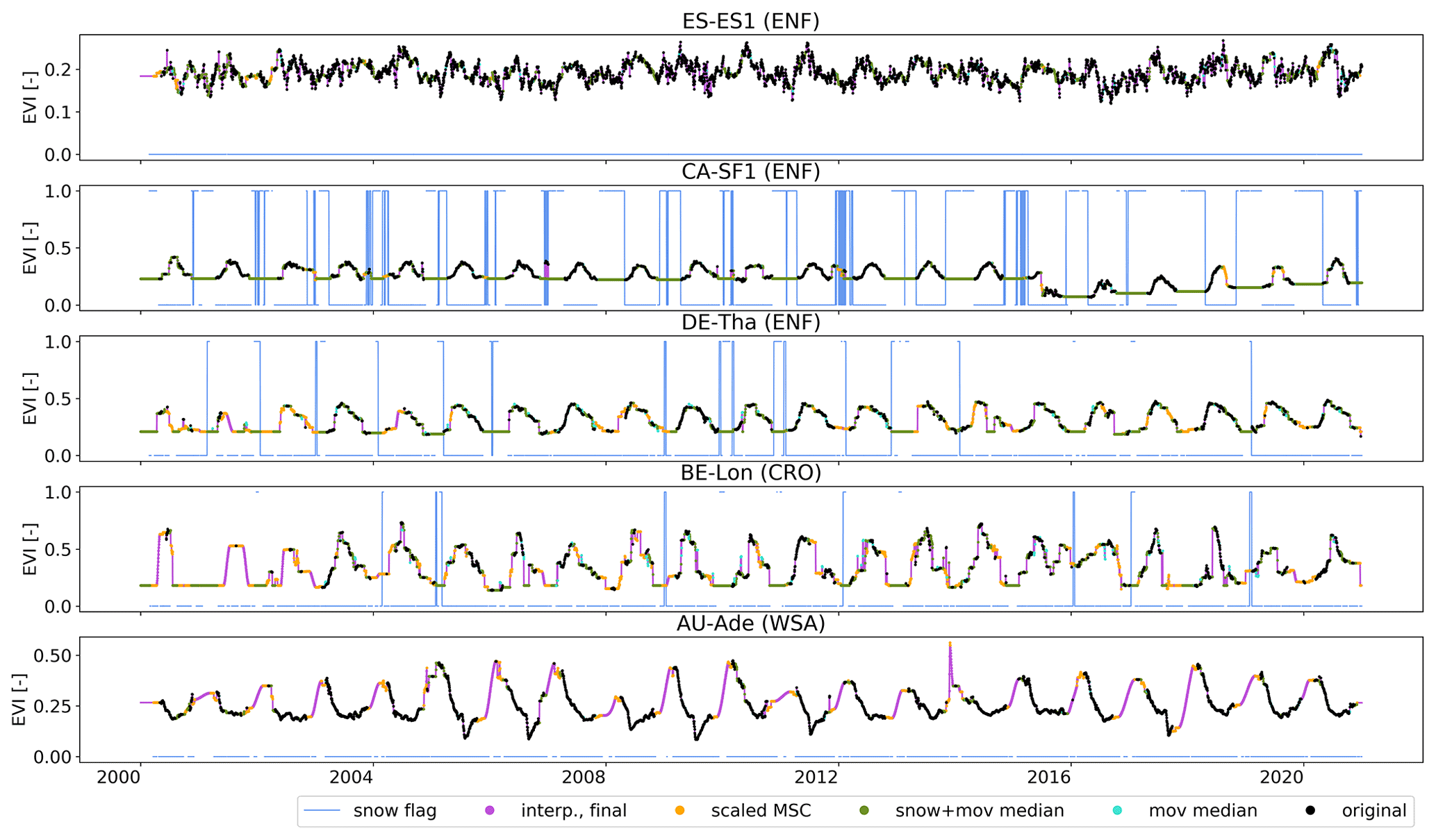
Figure 4 Illustration of gap-filling steps in the 500 m pixel containing selected eddy-covariance sites for the MODIS EVI.

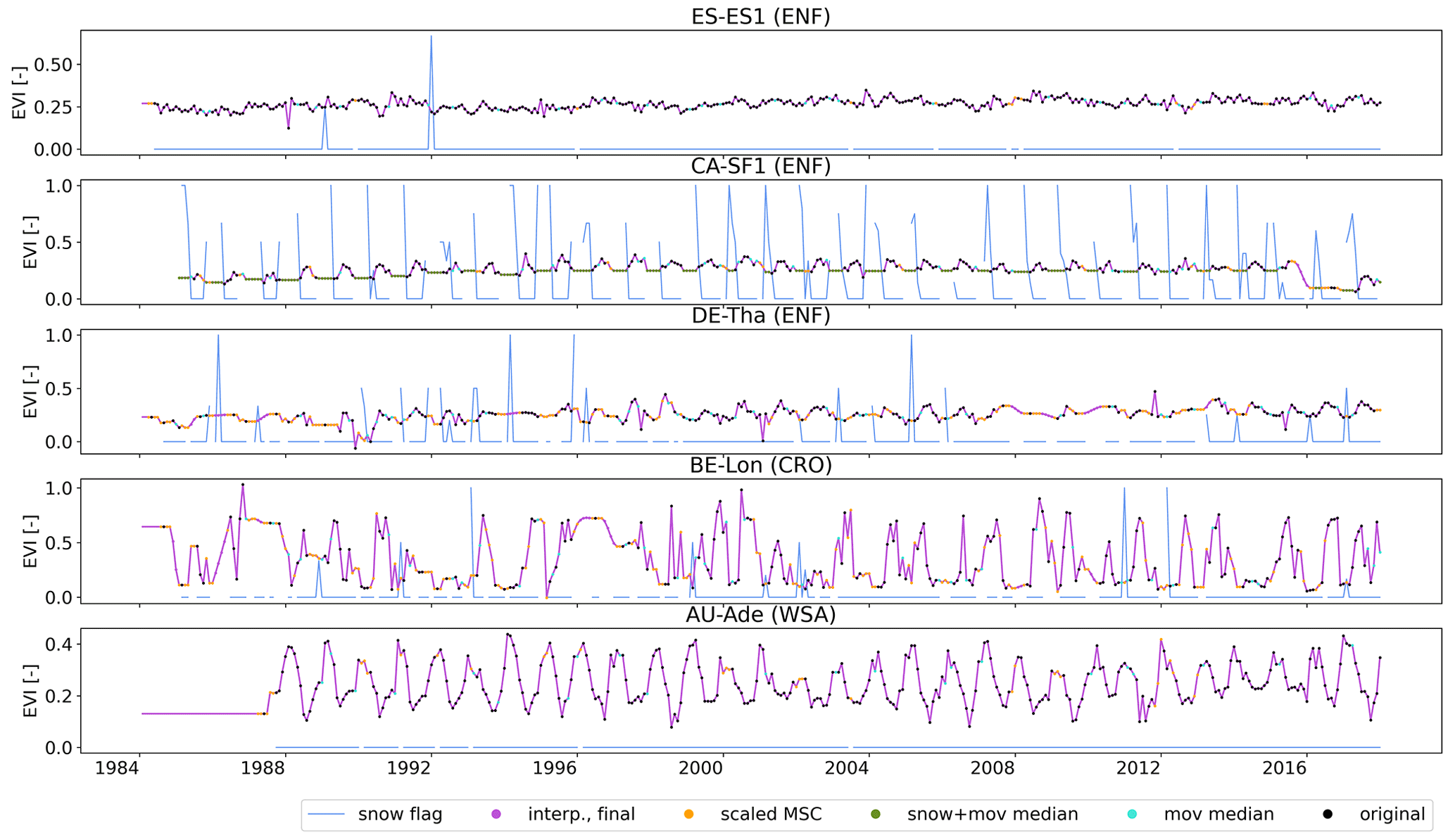
Figure 5 Illustration of gap-filling steps in the 30 m pixel containing selected eddy-covariance sites for the Landsat EVI.

Missing MODIS LST values were estimated most reliably in the gap-filling steps 1–2 (moving median and scaled average shift to observations at other overpass times) because the typical short-term variability in the time series could be preserved. In the Spanish site Majadas de Tiétar (ES-LMa, Fig. 6 top panel), savanna-type vegetation is prevalent with a dry summer and wet winter. Visually the gap-filling procedure succeeds in preserving the typical higher LST variability in the dry season and seasonally changing diurnal amplitudes. Also, in Saskatchewan (CA-SF1), gap-filling step 2 successfully estimates the largest fraction of missing values for each data stream from the complementary observation times. The EVI indicated a disturbance event at the beginning of 2015 (Fig. 4) that continued to strongly affect the EVI also in the following year. The event also marks the LST time series in that daytime LST, and therefore, the diurnal amplitude clearly increases in summer after 2015. The gap-filling procedure follows this behaviour. Relative to Majadas de Tiétar or Saskatchewan, in the mixed forest in Vielsalm (BE-Vie), data gaps are much more persistent throughout a day, and the gap filling works more often with the third gap-filling step using an average seasonal cycle of LST to estimate missing observations. Finally, at the woody savanna site Howard Springs in northern Australia (AU-How, Fig. 6 bottom panel) there is a strong seasonal phasing between daytime and nighttime LST. Data availability also changes with the seasons. In the monsoon season, synoptic variability in the filled data points is unrealistically low because the gap-filling needs to resort to filling by a median seasonal cycle of LST (obtained from those years in which the monsoon starts late) or by interpolation.

Geometrical corrections to the nadir viewing angle are much larger and have a stronger seasonality for daytime LST than for nighttime observations (rightmost panel in Fig. 6, Ermida et al., 2018). The daytime LST value from a nadir view is consistently estimated to be several kelvin higher than from an oblique view. The Australian Howard Springs site is an exception in that the correction offset to nadir has no consistent sign during the wet season.

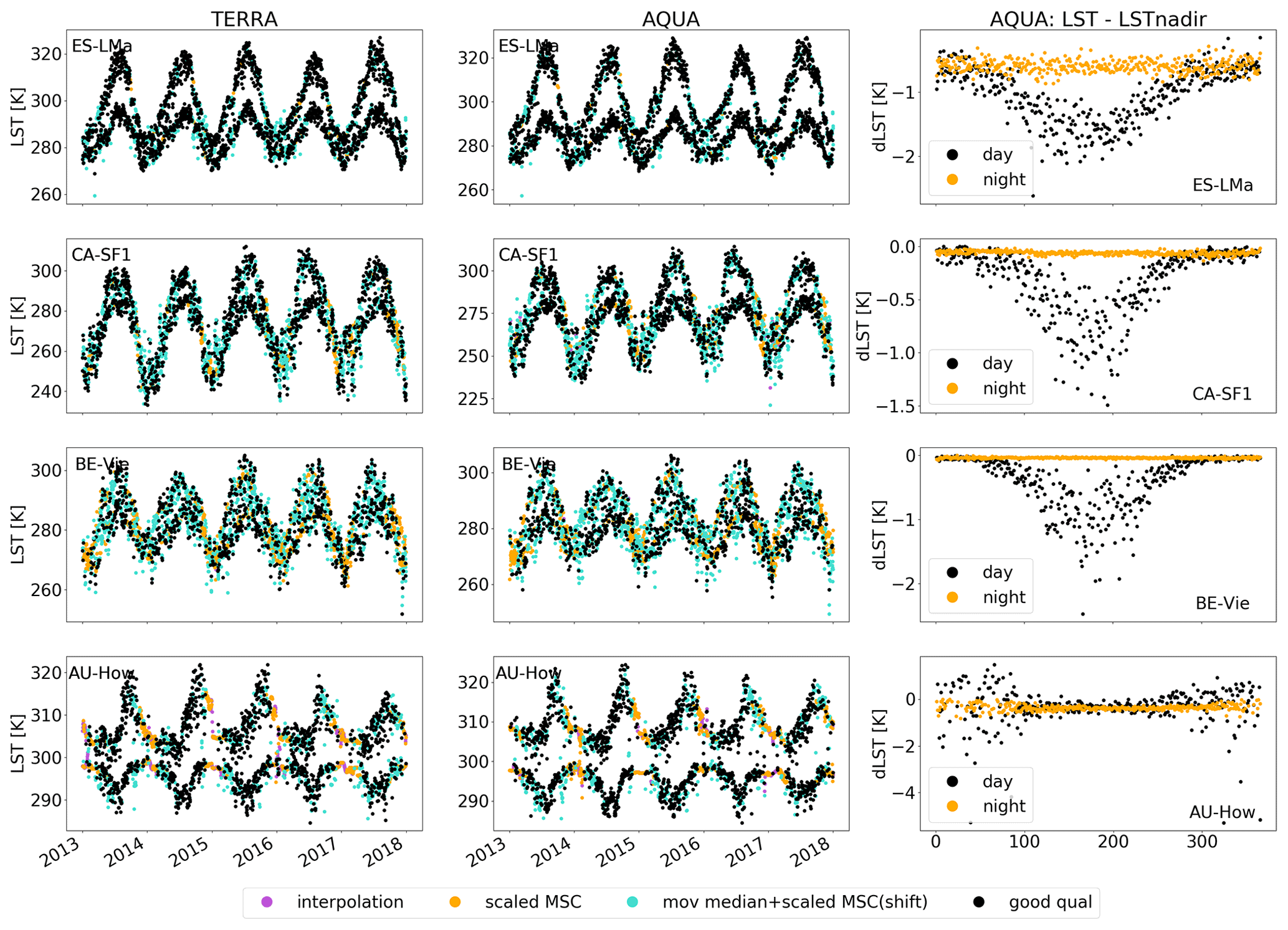
Figure 6 MODIS LST gap-filling steps in the 1 km pixel containing selected eddy-covariance sites for daytime and nighttime LST. The rightmost column shows the average annual cycle of the correction factor between LST from variable viewing angles and LST corrected to nadir view.

4.3 Benchmarking

In the experiments where artificial gaps are introduced at data points with known and valid values in the pixel containing the eddy-covariance site, FluxnetEO performance for MODIS is excellent with NSE values clearly above 0.9 for all reflectance-based indices, and even above 0.95 for artificial gap fractions of 20 % (Fig. C1 top left). The NSE of the gap-fill estimates for LST is systematically lower but above 0.8 and therefore still very good. Interestingly, the median NSE across sites is very similar for the 20 % and 40 % gap fraction experiments for the LST but clearly different for the reflectance. Overall, FluxnetEO outperforms missForest in the realism of the gap-fill estimates slightly but consistently across most reflectance-based MODIS variables, and more strongly so for the larger (and more realistic for the majority of sites) artificial gap fraction of 40 % (Fig. 7a). The NDWI variables are a special case, where missForest does not succeed in producing reliable estimates (Fig. C1b) and interestingly more so for low fractions of missing data. For LST, the ranking between missForest and FluxnetEO gap filling depends on the gap fraction: missForest consistently produces higher NSE for the lower gap fractions and FluxnetEO for 40 % of samples removed (Fig. 7a). For Landsat, the NSE of the gap-fill estimates in FluxnetEO is generally comparable to (derived vegetation indices) or better (spectral bands) than from missForest (Fig. 7b). The performance of FluxnetEO is more sensitive to the number of missing values than missForest (Fig. C1c, d). A few more points are of note: for both MODIS and Landsat, the gap-fill estimates of spectral surface reflectance in the visible range (blue, green, red) are less reliable than the one in channels with longer wavelength or derived vegetation indices. The overall gap-fill performance is not satisfactory for Landsat, either from FluxnetEO or from missForest. We did additional tests and found that the signal-to-noise ratio and the temporal resolution are decisive for the success of the gap filling. The time series of the average across all subpixels in the Landsat cutout exhibit less noise than the time series of the centre pixel, which also clearly increases the NSE of the artificial gap-fill estimates (Fig. C2a). FluxnetEO generally performs better on daily than on monthly data (see the lower NSE for MODIS at monthly resolution in Fig. C2b), which calls for attempts to improve the reliability of FluxnetEO at different temporal resolutions in future releases.

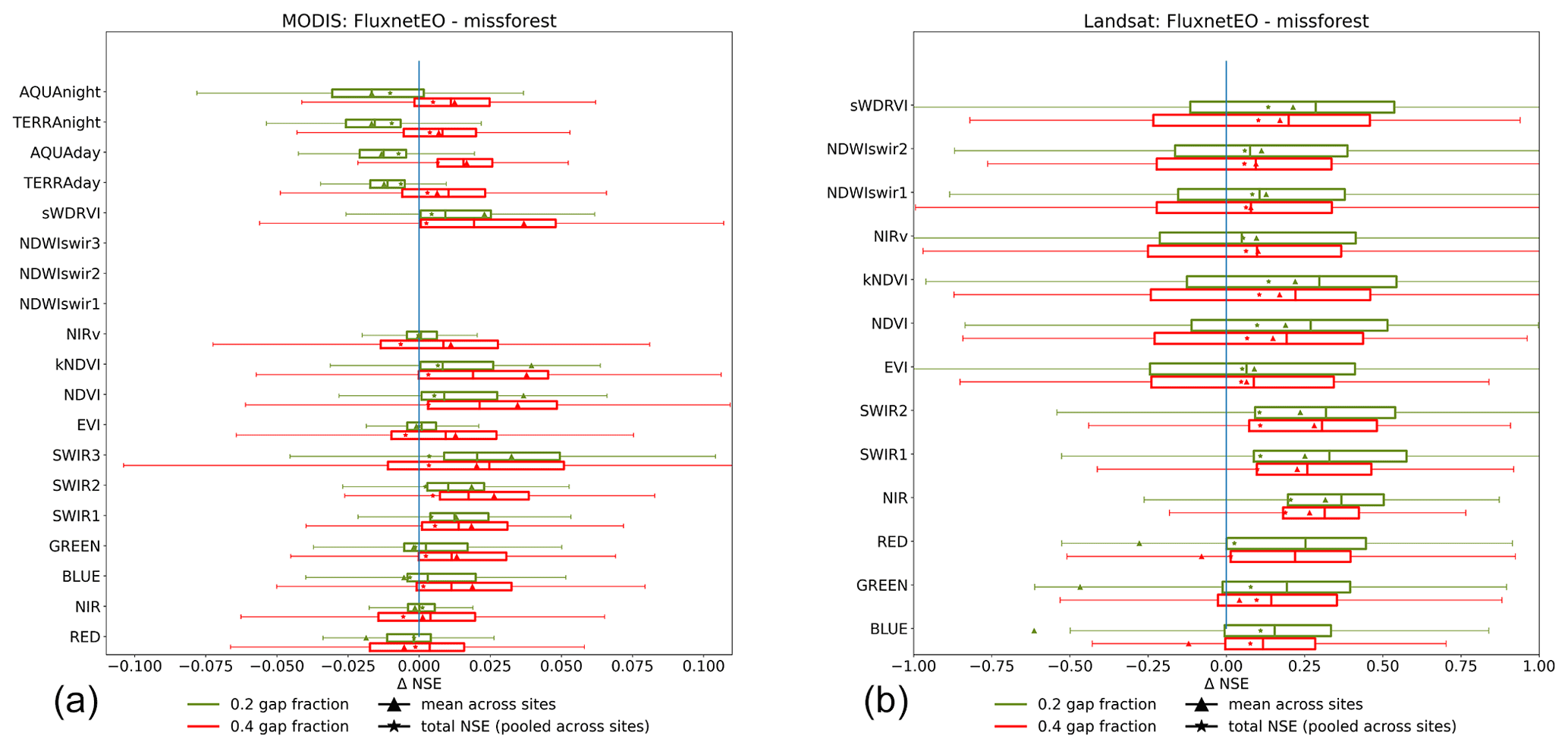
Figure 7 Benchmarking in artificial gaps: distribution of NSE per site of the gap-fill estimates in artificial gaps by FluxnetEO compared to missForest within the physical ranges of the indices for 20 % and 40 % of good-quality data removed. For MODIS (a) and Landsat (b), random good-quality samples are removed from the tower pixel.

Figure 8 compares the spatial and temporal patterns of Landsat NIR reflectance from FluxnetEO and Moreno-Martínez et al. (2020) across sites and shows a high consistency (panels a, b, d). The largest differences and lowest consistency in both spatial and temporal patterns happen outside the growing season (DJF in large parts of the CONUS, panels b, d, f). This can be expected as NIR reflectance is low during this time of the year, and because the treatment of snow and clouds differs between the products (see time series of one example site in Fig. C8). The temporal correlation of the deviations from the mean seasonality has a bimodal pattern with partly low Pearson correlations of under 0.5 (panel e). The consistency between FluxnetEO and Moreno-Martínez et al. (2020) surface reflectance products generally increases with wavelength, with the lowest agreement for the blue spectral band (Figs. C3, C4, C5, C6, C7).

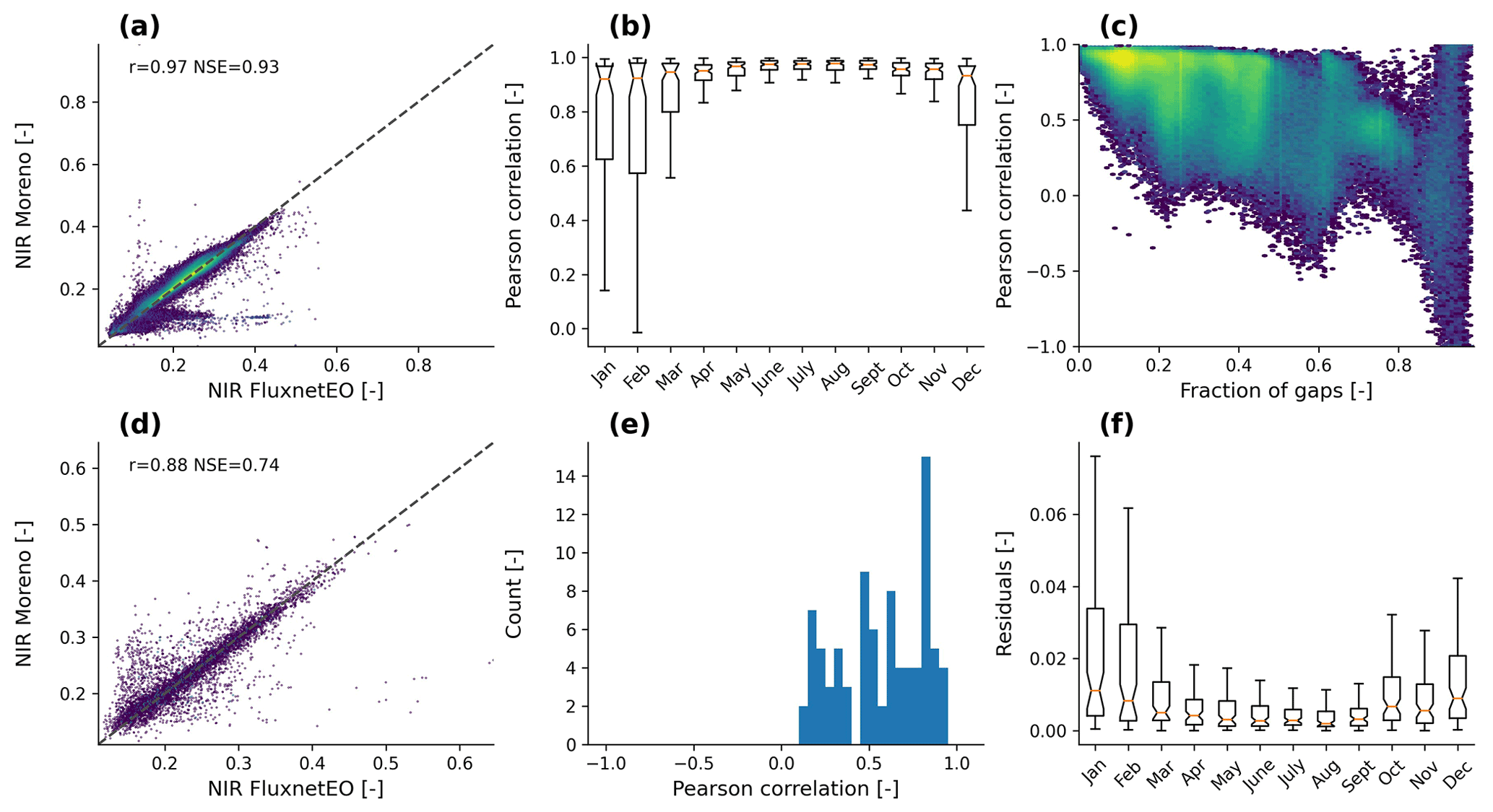
Figure 8 Benchmarking Landsat NIR reflectance from FluxnetEO against the product produced by Moreno-Martínez et al. (2020) at EC sites in the CONUS. Each sample NIR_s,t,p refers to one site (s), time step (t), and subpixel (p). Comparing spatial patterns: (a) scatterplot of the temporally averaged NIR reflectance (mean_t(NIR_s,p,t), each dot reflects one subpixel and site. (b) Temporal average across years for each month separately and the spatial Pearson correlation across all subpixels in a cutout per site and month cor_p(mean_t-month(NIR FluxnetEO_s,p,t), mean_t-month(NIR Moreno et al_s,p,t)). (c) Temporal correlation as a function of the number of missing values in the FluxnetEO product in each subpixel and site (cor_t(NIR FluxnetEO_s,t,p, NIR Moreno_s,t,p). (d–f) Compute a spatial average across all subpixels in a cutout per time step: NIR^*_s,t = mean_p(NIR_s,t,p). (d) Temporal Pearson correlation of the spatially averaged NIR (cor_t(NIR FluxnetEO^*_s,t, NIR Moreno^*_s,t). (e) Pearson correlation of the deviations from the mean seasonal cycle of the spatially averaged time series. (f) Difference between FluxnetEO and Moreno NIR reflectance and their average per month of the year mean_t-month(NIR FluxnetEO^*_s,t – NIR Moreno^*_s,t). r refers to the Pearson correlation coefficient and NSE to the Nash–Sutcliffe efficiency (Nash and Sutcliffe, 1970).

These benchmarking exercises illustrate important shortcomings but at the same time clearly support the quality of the gap-filling approach proposed by FluxnetEO as being comparable to or slightly higher than independent approaches and products. The artificial gaps at random positions in the first experiment might be comparable to those expected from bad inversion or clouds. Removing longer consecutive periods such as during snow periods or persistent cloud cover in rainy seasons is not feasible due to limited consecutive good-quality data, so we cannot test the performance for gaps of this type. Compared to missForest, FluxnetEO has the great advantage of being easily scalable to large-scale gridded data products. Compared to the product of Moreno-Martínez et al. (2020) FluxnetEO offers coverage at global sites and is not restricted to the CONUS but lacks the availability of gridded data.

4.4 On the importance of spatial context

In this section, we present different examples of the relevance of spatial context. The type and distribution of the vegetation around a given EC measurement station are not necessarily homogeneous. Instead, clusters of different vegetation or land use types might prevail in different sections of the immediate surroundings of a site. The area that a given flux measurement is representative of (the flux footprint, Schmid, 1997) changes rapidly with wind direction, turbulence conditions, atmospheric stability, and surface resistance (Schmid, 1997; Vesala et al., 2008; Chu et al., 2021). An exact match between the flux footprint and EO data (or a model grid cell) is challenging due to the often unknown or uncertain flux footprints and coarse spatial grid sizes. The scale mismatch is equally important for validation exercises for site-level measurements of surface reflectance (Romá et al., 2009; Cescatti et al., 2012), site-level energy-balance closure (Stoy et al., 2013), and model–data integration (Williams et al., 2009). The role that the scale mismatch between site-level and EO data plays for ecosystem analyses clearly depends on the site and the application. Some applications try to account for the mismatch (Pacheco-Labrador et al., 2017; Wagle et al., 2020); others ignore it and use a custom area around each EC site. Approaches to quantify and account for heterogeneity within a satellite pixel or a certain area around a given site do exist in the literature (Romá et al., 2009; Chu et al., 2021; Duveiller et al., 2021) but seem less exploited.

We computed the average flux footprints for every day (MODIS) and month (Landsat) around three example EC stations (Majadas de Tiétar, ES-LM1, Gebesee, DE-Geb, and Zotino, RU-Zo2). We illustrate how the relationship between EC-derived gross primary productivity (GPP) and EVI as an EO-derived proxy of the same changes according to whether the footprint area is taken into account or custom cutout sizes are chosen. In RU-Zo2, we compare surface temperature inverted from sensible heat flux to LST and illustrate how the pixel sizes relate to the flux footprint area (see details on the data processing in Appendix D).

The site ES-LM1 (El-Madany et al., 2018) is a tree–grass ecosystem. While the trees are evergreen, the herbaceous layer senesces in summer and re-greens in autumn (Luo et al., 2018). The EO cutout includes irrigated agricultural areas north of the flux footprint. These fields are barren in winter and are covered with crops in summer. MODIS and Landsat EVI are strongly negatively correlated to GPP derived from EC in the pixels over agricultural areas, as are the anomalies of EVI and GPP (Fig. D1a–d). Conversely, high positive correlations prevail across the remaining larger parts of the EO cutouts. Landsat EVI overlaid by the average flux footprint for two example months illustrates that the EC GPP is only representative of the tree–grass ecosystem (Fig. 9e, g). Hence, the spatial representativeness of EO data for EC fluxes might differ strongly depending on which satellite pixels are chosen for the analysis. We computed the average EVI that is representative of the flux footprint (henceforth fpa for footprint area). We compared it with an average EVI weighted with the probability density function of the flux footprint in order to take into account the decreasing influence of subpixels further away from the tower (henceforth fpw for weighted footprint area), as well as with two pragmatic approaches in case a flux footprint is unknown: an EVI average over all subpixels in the cutout with a radius of 2 km (henceforth fex for full extent) or only the single subpixel that contains the tower (cpx for centre pixel). The most noticeable difference between the time series for the different intersection methods is that the full extent (fex) in both Landsat and MODIS EVI is comparatively lower during the winter period (Fig. 9a,c). The agricultural areas contribute to fex, while the footprint intersection methods (fpa and fpw) and the centre pixel (cpx) EVI consistently indicate high greenness in the tree–grass ecosystem.

Gebesee, DE-Geb, is an agricultural site. The common approach in conducting EC measurements is to put the tower in a location where the land use is as homogeneous as possible, to be able to attribute fluxes to a targeted ecosystem, e.g. a known crop type. In Gebesee, this was assured for most of the years in the long site history (e.g. Fig. 9h), but not from 2011–2013. In these years, the field was split into two different adjacent crop types that contributed to the measured fluxes (Fig. 9f), raising the risk for pitfalls in the analyses of the fluxes. Also, in situations/years when the flux footprint represents a single field, additional potential difficulties originate from phenological differences between fields within the EO cutouts (Fig. 9f, h) if not properly matched. For example, the anomalies of both GPP and EVI are only highly correlated with each other in the immediate surroundings of the tower (Fig. D1g–h). Phenological heterogeneity between fields might explain why the EVI averaged over the full cutout (fex) is clearly different from the EVI in the footprint area (fpa, fpw) or the tower pixel (cpx) during the growing season maxima in 2015/2016 (Fig. 9b, d). Also, consistent with the GPP, the EVI in the tower pixel indicates slightly later senescence in 2017 than averaged over the footprint area or the full cutout, highlighting considerable effects of a mismatch between the flux footprint and the EO area.

Irrespective of the match between flux footprint and the area that the EVI is representative of, Fig. 9 illustrates the complimentarity between MODIS and Landsat in terms of resolution. Although Landsat offers high spatial detail, the temporal patterns that can be resolved with monthly averages are much coarser than the shorter variations that daily MODIS data can describe. Depending on the application, the user of FluxnetEO might choose one or the other.

Figure 9 Time series of EVI and GPP for ES-LM1 (a, c) and DE-Geb (b, d). MODIS EVI (a, b) and Landsat EVI (c, d) represent areas with different extents: full extent of the cutout (EVI_fex), the centre pixel that contains a tower (EVI_cpx), the EVI averaged over the flux footprint area (EVI_fpa), and the EVI_fpa weighted with the flux probability density function (EVI_fpw). Panels (e)–(h): Landsat EVI overlaid with the monthly flux footprint (black line) for ES-LM1 in November 2014 (e) and April 2016 (g) and for DE-Geb in February 2012 (f) and February 2016 (h). Non-original low-quality EVI values are blacked out. Red circles indicate the location of the EC station, and the white circle denotes 1 km diameter from the station.

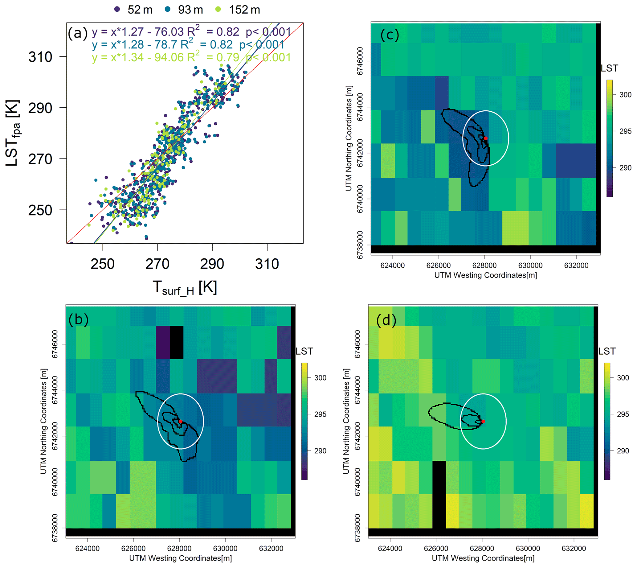
Figure 10 Relationship between MODIS AQUA_day LST_fpa and surface temperature (T_{surf_H}) calculated from the inverted sensible heat flux (details about the methods in Appendix D). The red line represents the 1:1 line. Panels (b) to (d) show example footprints at the three levels (black lines) overlaid on the LST map from 31 May to 2 June 2017, respectively. Non-original low-quality LST values are blacked out. The white circle indicates the 1 km diameter around the tower.

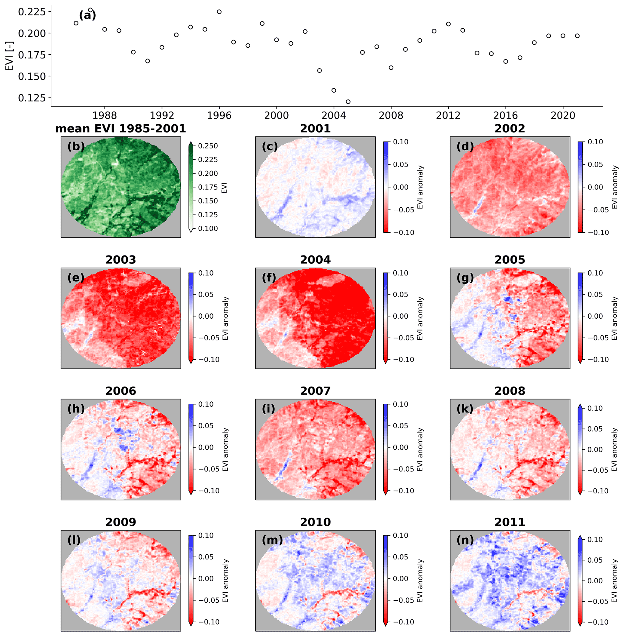
Figure 11 Annual EVI dynamics at the site US-SO₃ as observed by Landsat. Time series of spatial average annual EVI for the full 4×4 km² cutout (a) and the long-term temporal average spatial patterns of EVI (b). Annual anomalies of EVI for the period 2003–2011 in panels (c)–(n) (anomaly EVI${}_{=\mathrm{year}n}={\mathrm{EVI}}_{\mathrm{year}n}-\mathrm{mean}({\mathrm{EVI}}_{\mathrm{1985}-\mathrm{2001}}$)).

RU-Zo2, the Zotino tall tower observatory ZOTTO, is located in the taiga–tundra transition zone. The landscape in the proximity of the EC station is a heterogeneous mix of forest, bogs, and wetlands. At the tall tower, fluxes are measured at different heights above the canopy. The size of the flux footprint strongly increases with height, and the fluxes at the highest level partly represent areas more than 2 km away from the site (Fig. 10b–d). Flux footprints of measurements closer to the canopy are usually much smaller than the MODIS pixel size of 1 km for the LST, but the flux footprints of the higher measurement levels at RU-Zo2 partly integrate over multiple such pixels. Size and direction of the footprint extents strongly vary over time (note that Fig. 10b–d represent 3 consecutive days), such that the vegetation types and surface conditions sampled not only differ between measurement heights but also between days. We compare spaceborne LST AQUA_day integrated over the flux footprint area (LST_fpa) with surface temperature inverted from sensible heat flux measured at the tower for clear-sky days (Fig. 10a; see details about the methods in Appendix D). We observe a tendency of LST_fpa at all three measurement heights to be slightly lower than inverted surface temperature under freezing conditions with a notable scatter. For temperatures above 0 ^∘C, the scatter decreases, and LST_fpa of all three heights is consistently higher than the inverted surface temperature. For the peak surface temperatures during a year (above approximately 285 K), the slope between LST_fpa and surface temperature visually decreases, which might indicate significant changes in surface emissivity during the brief peak growing season when vegetation extent is highest and the surface has drained from snowmelt.

Next to matching the flux footprints with the EO data pixels, spatial context is equally important in studies of vegetation recovery after a disturbance event. The Sky Oaks-Young Stand (US-SO3) is a closed shrubland with less than 2 m tall woody vegetation. The US-SO3 site experienced a fire during the period 2002–2003, followed by regrowth. Landsat allows us to observe the impact structure and the spatially very heterogeneous recovery dynamics with remarkable detail (Fig. 11): the fire caused lower-than-average EVI in large parts of the cutout during the period 2002–2004 (Fig. 11d-f). From 2005 onwards, some patches, particularly the western part of the cutout, appear to have recovered faster from the disturbance than other patches (Fig. 11g). By 2011, EVI has reached pre-fire values in most parts of the area around the site with only small patches as exceptions indicating that regrowth was complete (Fig. 11n). This example illustrates how high-spatial-resolution EO combined with EC at the site level can provide complementary insights for better understanding disturbance regimes and the associated recovery dynamics.

5 Conclusions

The proposed methods aim at assuring good quality and producing as reliable as possible gap-free estimates of EO-derived surface reflectance, vegetation indices, and LST for pixels around EC sites, while remaining independent of additional data sources and being generalisable. Depending on the question/application at hand, either MODIS or Landsat EO data might be more suitable with their inherently very diverse spatial and temporal resolutions, reliability of the gap-filling approach, and temporal coverage. The requirements for the strictness of the quality checks and the sophistication of the gap-filling methods differ by use case. No approach can fit all requirements, but we expect FluxnetEO to offer many opportunities to advance our understanding of land–atmosphere fluxes for individual sites across regional networks and globally. It helps bridging the Fluxnet, remote sensing, and modelling communities and facilitates consistent benchmarking of EO-based flux models of any kind. We anticipate that this will accelerate our ability to monitor and understand land–atmosphere fluxes across spatial and temporal scales. For the future, we plan to maintain, update, and improve FluxnetEO. This will include extending the time series to the most recent years, adding EC sites as measurements become available in one of the networks, improving the processing based on newly identified drawbacks and/or user needs (e.g. Landsat sensors harmonisation, better performance also at lower temporal resolutions), and updating to new EO data collections (e.g. Landsat collection 2, integration of Landsat 9). Importantly, forthcoming FluxnetEO versions shall more strongly facilitate complementary usage of multiple missions to exploit their synergy potential, so that future additions will include further EO products, for example the Sentinel missions. Although temporal overlap with most of the EC records is low, it will grow with the lifetime of the different Sentinel missions because strong efforts in the EC community target the timely, free, and open distribution of site-level measurements.

Appendix A: Technical details about the processing of surface reflectance

In this section we provide all specific technical details necessary to reproduce our processing steps for the surface reflectance of MODIS and Landsat.

The quality control of the MODIS reflectance-based land surface indicators included the following steps.

• Omission of the MCD43A2 BRDF_Albedo_Band_Quality_BandX flags ≥ 3 for each band to remove bad inversion quality from the surface reflectances.

• The flag Snow_BRDF_Albedo eliminated pixels that contain snow. As the gap-filling procedure used the snow information, a spatially aggregated snow flag was needed for the processing version that averages valid data within 1 km of the tower. For this, we defined the aggregated snow flag as the fraction of subpixels in the cutout that are snow covered. If more than 50 % of subpixels have missing snow information for a certain day, the aggregated snow flag is set to missing as well.

• The presence of water in a scene seen by an optical sensor can strongly affect the observation. The BRDF_Albedo_LandWaterType flag allowed us to filter for pixels exclusively on land (flag = 1). This eliminated all data for many Swiss, Dutch, Italian, and Finnish sites which are situated close to water bodies. Inclusion of ocean coastlines and lake shorelines (flag = 2) and shallow inland water (flag = 3) resulted in reasonable time series at most sites. This came at the cost of having a few other sites that were affected by the presence of water. As a trade-off between data availability and quality, we decided to include land–water flags 1–3.

• After the computation of the vegetation indices from the individual spectral bands, an additional check removed possible values of the spectral vegetation indices outside their defined ranges. An outlier filter compared each value to the median of all valid values in temporal windows of 30 d (Papale et al., 2006). A large difference of a given value to the median of its surrounding values indicates a potential outlier. The threshold z as in Papale et al. (2006) was set to 2, and only a less conservative threshold of z=3 acted when more than 20 valid values were available in a given window.

Robinson et al. (2017)Moreno-Martínez et al. (2020)Sun et al. (2017)ORNL DAAC (2018)

Table A1 FluxnetEO compared to a selection of other products and services featuring Landsat and MODIS EO data.

The empirical outlier filter for Landsat slightly differed from the one for MODIS and removed observations in the five highest and lowest percentiles of the median seasonal cycle of an index if they differed more than 75 % from their surrounding 3-month moving window median. The second criterion was critical in order to preserve observations of disturbance events or recovery dynamics.

Technical details for the gap filling are as follows.

• 1.

  The first step is a moving window median to fill short non-snow-related gaps. If the entire time series has less than 40 % valid data, a given moving window contains both the actual values and the median seasonal cycle for the given time of the year. The median for the moving window then refers to the distribution of both.

• 2.

  The second step fills reflectance values with a constant value in the presence of snow (snow flag ≥ 0.1). Partly long periods with missing snow information in the Snow_BRDF_Albedo flag needed special treatment. Some of these gaps appeared systematically in early winter in higher latitudes, so times of missing snow information are also considered as snow covered. However, also during the growing season long periods of missing snow information occur at several sites globally. The following criteria check whether a period that is considered snow covered by high values or missing snow flags is filled with a constant baseline value or not.

  • –

    If a given site has fewer than 60 d (10 months for Landsat) with valid snow coverage (i.e. Snow_BRDF_Albedo=1) in the total record, snow typically does not occur at the site. In this case the gap-filling procedure does not apply this gap-filling step at all for this site.

  • –

    The gap filling with a constant value only addresses gaps with a minimum length of 20 consecutive days (1 month for Landsat) with snow flag missing or 1. This avoids filling very short intermittent snow periods or short gaps in snow information during the growing season.

  • –

    This gap-filling step does not consider gaps due to missing snow information if the median seasonal cycle of snow coverage indicates ≤ 5 % of snow cover at the given time of the year and the difference between the fill value and the median seasonal cycle is large (i.e. exceeds the 85th percentile of the differences in times of missing snow information).

  The constant baseline value that is used to fill snow periods in the time series for a site represents the third percentile of the median seasonal cycle of the spectral vegetation indices. If a given index typically has high values outside the growing season, the baseline value represents the 97th percentile instead. However, if for a given winter the average over the last five (one observation for Landsat) valid data points at the end of the growing season or over the first five valid data points at the beginning of the next growing season is lower than the baseline value (higher than the baseline for indices which are typically high outside the growing season), the baseline takes the value of this average for the given winter (similar to  Beck et al., 2007).

• 3.

  Linearly scale the median seasonal cycle (MSC) to the time series to fill longer gaps (Verger et al., 2013). Calibration happens in moving temporal windows of 80 d (24 months for Landsat) and application of the scaling in steps of 20 d (4 months for Landsat). In the following x represents a time series of reflectance-based indices and x^* the time series with some of its gaps filled by a scaled MSC.

  $$\begin{array}{c}{\displaystyle }{\mathit{x}}_{t=k:k+\mathrm{80}}=f\left(\mathrm{MSC}(\mathit{x}{)}_{t=k:k+\mathrm{80}}\right)\\ {\displaystyle }{\mathit{x}}_{t=k:k+\mathrm{20}}^{*}=m\cdot \mathrm{MSC}(\mathit{x}{)}_{t=k:k+\mathrm{20}}+n\end{array}$$

Appendix B: Technical details about the processing of MODIS LST

In this section we provide all specific technical details necessary to reproduce the processing steps for the MODIS LST.

The empirical filter to remove potential outlier values (Papale et al., 2006) followed the same procedure as for the vegetation indices but used a constant z value of 1.5 as it provided the best trade-off between filter success, false positives, and false negatives.

Estimates of LST in data gaps originate from the following steps.

• –

  In contrast to the procedure for the reflectance-based vegetation indices, the distribution of values in the temporal windows of 8 d is not supplied by the median seasonal cycle in case of low data availability. The moving window median was not applied for windows with fewer than three valid values.

• –

  Filling by linearly scaling the median seasonal shift between any two of the four MODIS LST time series to each other (Crosson et al., 2012; Li et al., 2018). The following explains this gap-filling step for TERRA_day as the “imputed” time series.

  • 1.

    Compute the shift between TERRA_day and AQUA_day (Δ(TERRA_day, AQUA_day)) and obtain the MSC of the shift: MSC(Δ(TERRA_day, AQUA_day)).

  • 2.

    Linearly scale the MSC of the shift to the shift itself in temporal windows of 80 d (provided a minimum of 10 valid values in a given window). Apply the scaling in windows and steps of 20 d to obtain estimates of the shift (Δ(TERRA_day, AQUA_day)^*) from its MSC where it is missing.

    $$\begin{array}{c}{\displaystyle }\mathrm{\Delta }{\left({\mathbf{TERRA}}_{\mathrm{day}},{\mathbf{AQUA}}_{\mathrm{day}}\right)}_{t=k:k+\mathrm{80}}\\ {\displaystyle }=f\left(\mathrm{MSC}{\left(\mathrm{\Delta }\left({\mathbf{TERRA}}_{\mathrm{day}},{\mathbf{AQUA}}_{\mathrm{day}}\right)\right)}_{t=k:k+\mathrm{80}}\right)\\ {\displaystyle }\mathrm{\Delta }{\left({\mathbf{TERRA}}_{\mathrm{day}},{\mathbf{AQUA}}_{\mathrm{day}}\right)}_{t=k:k+\mathrm{20}}^{*}\\ {\displaystyle }=m\cdot \mathrm{MSC}{\left(\mathrm{\Delta }\left({\mathbf{TERRA}}_{\mathrm{day}},{\mathbf{AQUA}}_{\mathrm{day}}\right)\right)}_{t=k:k+\mathrm{20}}\\ {\displaystyle }+n\end{array}$$
  • 3.

    Add the scaled average shift to the AQUA_day to obtain an estimate of ${\mathrm{TERRA}}_{\mathrm{day}}^{*}\left[{\mathrm{AQUA}}_{\mathrm{day}}\right]$ that can fill gaps in TERRA_day.

    $$\begin{array}{c}{\displaystyle }{\mathbf{TERRA}}_{\mathrm{day}t=k:k+\mathrm{20}}^{*}\left[{\mathbf{AQUA}}_{\mathrm{day}}\right]\\ {\displaystyle }={\mathbf{AQUA}}_{\mathrm{day}t=k:k+\mathrm{20}}\\ {\displaystyle }+\mathrm{\Delta }{\left({\mathbf{TERRA}}_{\mathrm{day}},{\mathbf{AQUA}}_{\mathrm{day}}\right)}_{t=k:k+\mathrm{20}}^{*}\end{array}$$

  Analogously to TERRA${}_{\mathrm{day}}^{*}$[AQUA_day], the night-time LST observations also contributed to estimate TERRA${}_{\mathrm{day}}^{*}$[TERRA_night] and TERRA${}_{\mathrm{day}}^{*}$[AQUA_night]. All three estimates, TERRA${}_{\mathrm{day}}^{*}$[AQUA_day], TERRA${}_{\mathrm{day}}^{*}$[TERRA_night], and TERRA${}_{\mathrm{day}}^{*}$[AQUA_night], served to fill gaps in TERRA_day, namely in the order of increasing standard deviation of the differences between valid TERRA_day and each of the three estimated TERRA${}_{\mathrm{day}}^{*}$ values.

  The procedure analogously filled AQUA_day, TERRA_night, and AQUA_night accordingly using valid observations of the remaining three, respectively.

• –

  Linearly scale the valid LST observations of each of the four data streams to their own median annual cycle in temporal windows. As in step 2, the calibration happened in temporal windows of 80 d, while the scaling was applied in windows of 20 d. Exemplarily for TERRA_day.

  $$\begin{array}{c}{\displaystyle }{\mathbf{TERRA}}_{\mathrm{day}t=k:k+\mathrm{80}}=f\left(\mathrm{MSC}{\left({\mathbf{TERRA}}_{\mathrm{day}}\right)}_{t=k:k+\mathrm{80}}\right)\\ {\displaystyle }\begin{array}{rl}{\mathbf{TERRA}}_{\mathrm{day}t=k:k+\mathrm{20}}^{*}& =m\cdot \mathrm{MSC}{\left({\mathbf{TERRA}}_{\mathrm{day}}\right)}_{t=k:k+\mathrm{20}}\\ & +n\end{array}\end{array}$$

Appendix C: Details about the benchmarking exercises

Figure C1 Benchmarking in artificial gaps: distribution of NSE per site of the gap-fill estimates in artificial gaps by FluxnetEO (a, c) and missForest (b, d) within the physical ranges of the indices for 20 % and 40 % of good-quality data removed. For MODIS (a, b) and Landsat (c, d), random good-quality samples are removed from the tower pixel. Note the different x-axis limits.

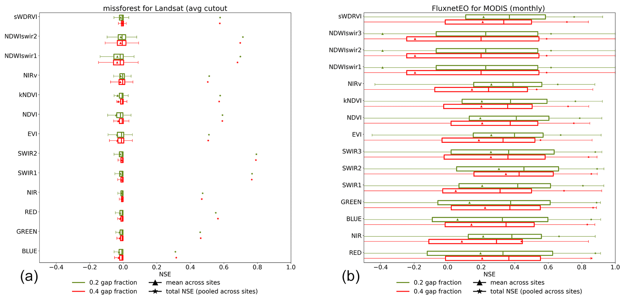
Figure C2 Benchmarking in artificial gaps: distribution of NSE per site of the gap-fill estimates in artificial gaps by FluxnetEO. A total of 20 % and 40 % of data were removed and gap-filled. (a) Landsat time series of the average reflectance/vegetation index across the whole cutout. (b) The centre pixel of MODIS data aggregated to monthly temporal resolution.

Figure C3 Benchmarking Landsat reflectance in the blue spectral band from FluxnetEO against the product produced by Moreno-Martínez et al. (2020) at EC sites in the CONUS. Each sample reflectance_s,t,p refers to one site (s), time step (t), and subpixel (p). Comparing spatial patterns: (a) scatterplot of the temporally averaged reflectance (mean(reflectance_s,p)_t); each dot reflects one subpixel and site. (b) Spatial Pearson correlation across all subpixels in a cutout per site of the average grouped by month. (c) Temporal correlation as a function of the number of missing values in each subpixel and site. (d–f) Compute a spatial average across all subpixels in a cutout per time step. (d) Temporal Pearson correlation of the spatial average. (e) Pearson correlation of the deviations from the mean seasonal cycle of the spatially averaged time series. (f) Difference between FluxnetEO and Moreno reflectance and their average per month of the year. r refers to the Pearson correlation coefficient and mef to the Nash–Sutcliffe efficiency (Nash and Sutcliffe, 1970).

Figure C4 Same as Fig. C3 but for the green spectral band.

Figure C5 Same as Fig. C3 but for the red spectral band.

Figure C6 Same as Fig. C3 but for the first shortwave infrared spectral band.

Figure C7 Same as Fig. C3 but for the second shortwave infrared spectral band.

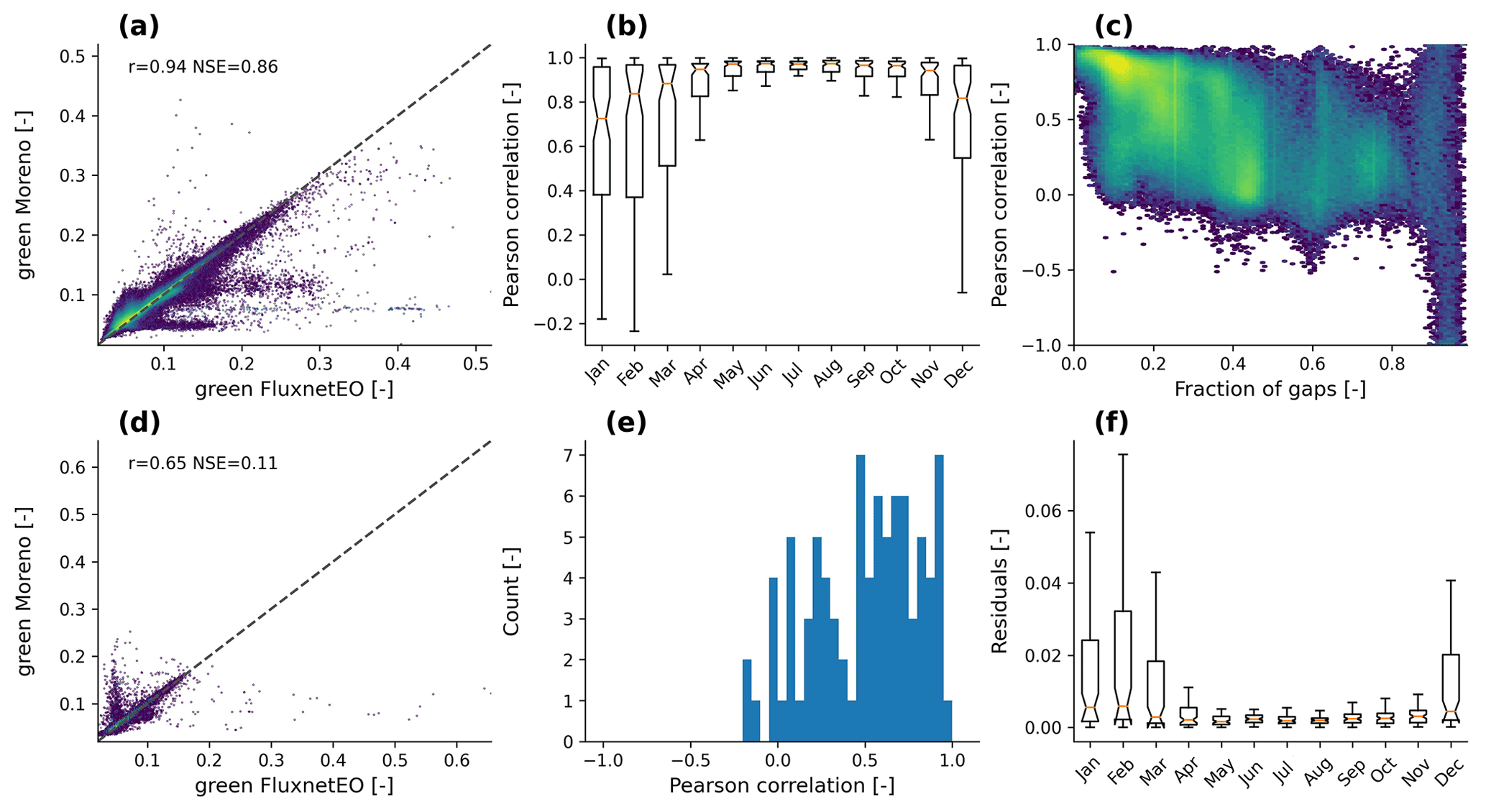
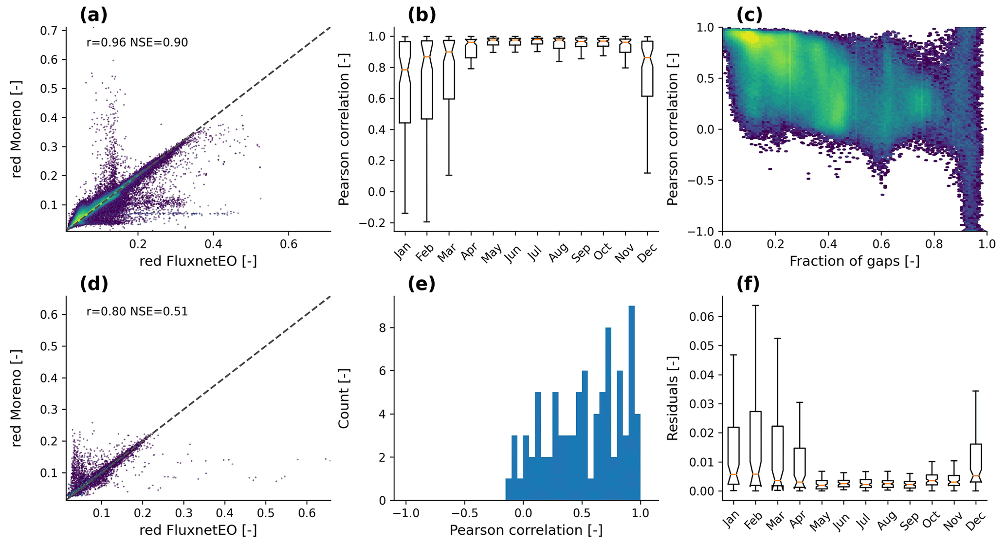
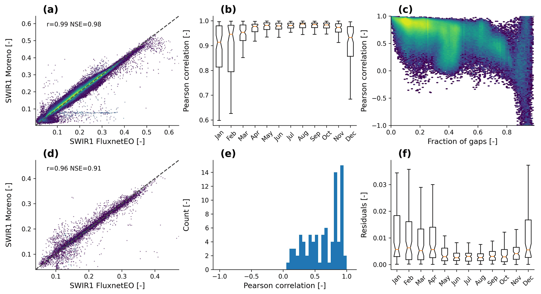
Figure C8 Example site US-Fmf: comparing the gap-filled surface reflectance products in spectral channels.

Appendix D: Details about the analysis of spatial context

For the analysis at DE-Geb and ES-LM1 we used night-time partitioned GPP (Reichstein et al., 2005) with the mean of the variable u^* threshold (GPP_NT_VUT_MEAN) from the Drought 2018 Team and ICOS Ecosystem Thematic Centre (2020) data release (Migliavacca et al., 2020; ICOS Ecosystem Thematic Centre and Gebesee, 2019). We computed the actual flux footprints after Kljun et al. (2015) from ICOS drought 2018 data (Drought 2018 Team and ICOS Ecosystem Thematic Centre, 2020) using the R-code version (V1.41) of the FFP tool. As a flux footprint for the intersection with EVI, we define the area that contributes 80 % to the flux footprint probability density function (80 % isoline of the monthly/daily cumulative flux footprint for Landsat and MODIS, respectively).

Flux footprint calculation followed the same procedure for the three measurement heights at RU-Zo2. Surface temperature was inverted from sensible heat flux and meteorological variables (Knauer et al., 2018) with the following equation:

$$\begin{array}{}\text{(D1)}& T_{\mathrm{surf}}=T_{\mathrm{air}}+H/\left(\mathit{\rho }\cdot c_{\mathrm{p}}\cdot G_{\mathrm{ah}}\right),\end{array}$$

with T_air the air temperature at measurement height (K), H the sensible heat flux (W m⁻²), ρ the density of air (kg m⁻³), c_p the specific heat capacity of the air (J kg⁻¹ K⁻¹), and G_ah the aerodynamic conductance to heat (m s⁻¹). G_ah is defined as $G_{\mathrm{ah}}=\mathrm{1}/({\mathrm{Ra}}_{\mathrm{m}}+{\mathrm{Rb}}_{\mathrm{h}})$, with the aerodynamic resistance to momentum Ra${}_{\mathrm{m}}=\mathit{u}/u^{*\mathrm{2}}$ and the canopy boundary layer resistance for heat Rb${}_{\mathrm{h}}=\mathrm{6.2}\times u^{*-\mathrm{2}/\mathrm{3}}$. As the inverted surface temperature was compared to LST AQUA_day, the average of half-hourly sensible heat flux of the nominal overpass time at 1.30 ± 1.5 h was taken. Only days with good quality in both the LST and sensible heat flux are used according to the following criteria: (i) more than 90 % of the EO cutouts have valid (i.e. non-gap-filled) values, which restricts the comparison to clear-sky conditions, and (ii) at least 50 % of the half-hourly long-wave fluxes and all meteorological data in a given day are of good quality. A larger cutout of 5×5 km² was extracted for MODIS LST to fully also cover the extent of the flux footprint of the highest measurement level but is used only for illustrative purposes and not in the data provided in the FluxnetEO collections.

Figure D1 Spearman correlation between EVI and GPP using monthly Landsat (a, c, e, g) and daily MODIS (b, d, f, h) data for ES-LM1 (a–d) and DE-Geb (e–h) Fluxnet sites. The correlation estimates were computed on the raw time series (a, b, e, f) and on the anomalies (c, d, g, h).

Appendix E: Site selection

Table E1 Sites in FluxnetEO product version 1.0: site codes and coordinates (rounded to four decimals). Site codes including a ^* indicate sites for which currently only MODIS data are provided.