On the impact of canopy model complexity on simulated carbon, water, and solar-induced chlorophyll fluorescence fluxes

Lack of direct carbon, water, and energy flux observations at global scales makes it difficult to calibrate land surface models (LSMs). The increasing number of remote-sensing-based products provide an alternative way to verify or constrain land models given their global coverage and satisfactory spatial and temporal resolutions. However, these products and LSMs often differ in their assumptions and model setups, for example, the canopy model complexity. The disagreements hamper the fusion of global-scale datasets with LSMs. To evaluate how much the canopy complexity affects predicted canopy fluxes, we simulated and compared the carbon, water, and solar-induced chlorophyll fluorescence (SIF) fluxes using five different canopy complexity setups from a one-layered canopy to a multi-layered canopy with leaf angular distributions. We modeled the canopy fluxes using the recently developed land model by the Climate Modeling Alliance, CliMA Land. Our model results suggested that (1) when using the same model inputs, model-predicted carbon, water, and SIF fluxes were all higher for simpler canopy setups; (2) when accounting for vertical photosynthetic capacity heterogeneity, differences between canopy complexity levels increased compared to the scenario of a uniform canopy; and (3) SIF fluxes modeled with different canopy complexity levels changed with sun-sensor geometry. Given the different modeled canopy fluxes with different canopy complexities, we recommend (1) not misusing parameters inverted with different canopy complexities or assumptions to avoid biases in model outputs and (2) using a complex canopy model with angular distribution and a hyperspectral radiation transfer scheme when linking land processes to remotely sensed spectra.

1 Introduction

Land surface models (LSMs) simulate the carbon, water, and energy fluxes at the land–atmosphere interface at regional and global scales and are a key component for Earth system models (ESMs). The ability of LSMs to accurately model the carbon, water, and energy fluxes within vegetation canopy largely determines the predictive skills of the ESMs. Modeling canopy carbon, water, and energy fluxes dates back to the early 20th century, and various canopy models have different complexities from a single layer to multiple layers (see Bonan et al., 2021, for an overview). To date, the most widely used canopy models in the LSM community are the “big-leaf model family”.

It should be noted that a big-leaf model may refer to different models within the last decades given their interchangeable uses (Luo et al., 2018). According to Luo et al. (2018), the big-leaf model can be categorized at least as the following types given the purposes for which they were developed. (1) The one-big-leaf canopy model considers a canopy to be a single big leaf and was typically used with the Penman–Monteith equation (Penman, 1948; Monteith, 1965) to compute land surface evaporation in early LSMs. Sellers et al. (1992) updated the one-big-leaf model by adding an exponentially diminishing photosynthetic rate within the canopy depth to upscale photosynthesis for the carbon–water coupled LSMs. Yet, this scheme often underestimated the canopy assimilation rate, as the exponential function cannot properly represent the vertical light and photosynthesis profiles. (2) A two-leaf radiation scheme separates the canopy into a group of sunlit leaves and a group of shaded leaves (Norman, 1982; De Pury and Farquhar, 1997; Campbell and Norman, 1998; Chen et al., 1999) and was used to account for the horizontal and vertical light heterogeneity in the canopy. (3) A two-big-leaf canopy model combines the one-big-leaf canopy model and two-leaf radiation scheme to upscale carbon and water fluxes and treats each of the sunlit and shaded fractions as a single big leaf, where leaf biochemical parameters and radiation are upscaled to the canopy level (De Pury and Farquhar, 1997; Wang and Leuning, 1998). (4) A two-leaf canopy model uses a two-leaf radiation scheme and treats each of the sunlit and shaded fractions as a leaf with average traits for its representation (not an integrated value as in a big leaf) (Chen et al., 1999, 2012; Sprintsin et al., 2012). Therefore, one needs to be cautious when using the term big-leaf model, as it may refer to (i) a two-leaf radiation scheme which is a canopy radiative transfer model or (ii) upscaling schemes which differ in the way leaf biochemical parameters are integrated (such as the one-big-leaf and two-big-leaf models) or averaged (such as the two-leaf canopy model).

The biggest advantage of the big-leaf model family is computational efficiency given the simple mathematical formulation. The potential disadvantages of the big-leaf model family are also obvious; e.g., the model is too simplified and thus not able to resolve vertically varying profiles and microclimates in the canopy, such as air temperature, humidity, and wind speed (Bonan et al., 2021). Thus, there is an increasing demand for LSMs to move from a simple one-layered canopy to a multi-layered one.

One of the most important functions of canopy models is to predict carbon, water, and energy fluxes globally in the future to determine whether the land will remain a carbon sink. Though canopy models with different complexity levels have been extended to a global scale in different LSMs, researchers are facing a key problem: a lack of direct global-scale carbon, water, and energy flux observations. The lack of data makes it difficult to calibrate the LSMs at global scales, particularly those using more complex canopy setups given the more parameters required. As a result, though it is shown that a multi-layered canopy model better resolves energy fluxes in the canopy (Bonan et al., 2021), little is known about whether the multi-layered canopy models show improved predictive skills (particularly in terms of carbon and water fluxes) compared to the big-leaf models which are widely used in existing LSMs.

To better constrain LSMs with data, people realized the promise of remote sensing data given their global coverage and satisfactory spatial and temporal resolutions. Regarding carbon, research has shown that solar-induced chlorophyll fluorescence (SIF) and the near-infrared reflection of vegetation (NIRv) are correlated with plant gross primary productivity (GPP; Frankenberg et al., 2011; Zhang et al., 2016; Sun et al., 2018; Badgley et al., 2019). Regarding water, researchers also found SIF to be useful for inverting the transpiration rate by prescribing stomatal responses to the environment (e.g., Shan et al., 2021) and the vegetation optical depth to be useful in sensing aboveground biomass and canopy water stress (Momen et al., 2017; Zhang et al., 2019). Regarding energy, various models and algorithms have been used to detect the surface energy balance using optical light and microwaves (e.g., Roerink et al., 2000; Norman et al., 2003). Further, methods and applications have been developed to invert plant traits from remote sensing data, such as leaf area index (e.g., Colombo et al., 2003; Deng et al., 2006) and chlorophyll content (Croft et al., 2020).

Despite the increasing number of inverted fluxes and plant trait datasets, there is limited research into testing the capability of these data in improving LSM predictions. Among the various reasons that hamper the fusion of large-scale datasets into LSMs, incompatibility between model and data assumptions seems to be the major reason. For example, the disagreement in canopy complexity may introduce errors into modeling if one uses the data inverted from a canopy complexity level (e.g., one-layered canopy) in a model with a different canopy complexity level (e.g., multi-layered canopy). Further, the flux and trait maps inverted from remote sensing data often use simplified plant physiological representations, which are, however, key processes in land modeling. For example, studies that derive GPP from SIF or NIRv often assume linear correlation between them, whereas vegetation models must account for light saturation (Zhang et al., 2016).

Ideally, LSMs can be constrained using raw reflection and fluorescence spectra. This, nevertheless, requires the LSMs to move from broadband canopy radiation to a hyperspectral representation and from sunlit and shaded fractions to leaf angular distributions (such as the land model developed by Climate Modeling Alliance, CliMA Land; Wang et al., 2021b). This way, the LSM can be directly coupled to remotely sensed canopy spectra (e.g., Shiklomanov et al., 2021) rather than to reprocessed datasets using often incompatible assumptions. The increasing canopy complexity, however, comes with high costs: (a) many more computational resources are required by the increasing number of leaves (e.g., CliMA Land canopy has a default of 6500 leaves per tree in the canopy, whereas a two-leaf canopy has two “leaves”); (b) canopy radiation and fraction (e.g., the CliMA Land model calculates the radiation and fraction based on leaf angular distribution for a default of 6500 leaves) are more complicated; and (c) most importantly, there is increasing difficulty for research communities when understanding or using the model.

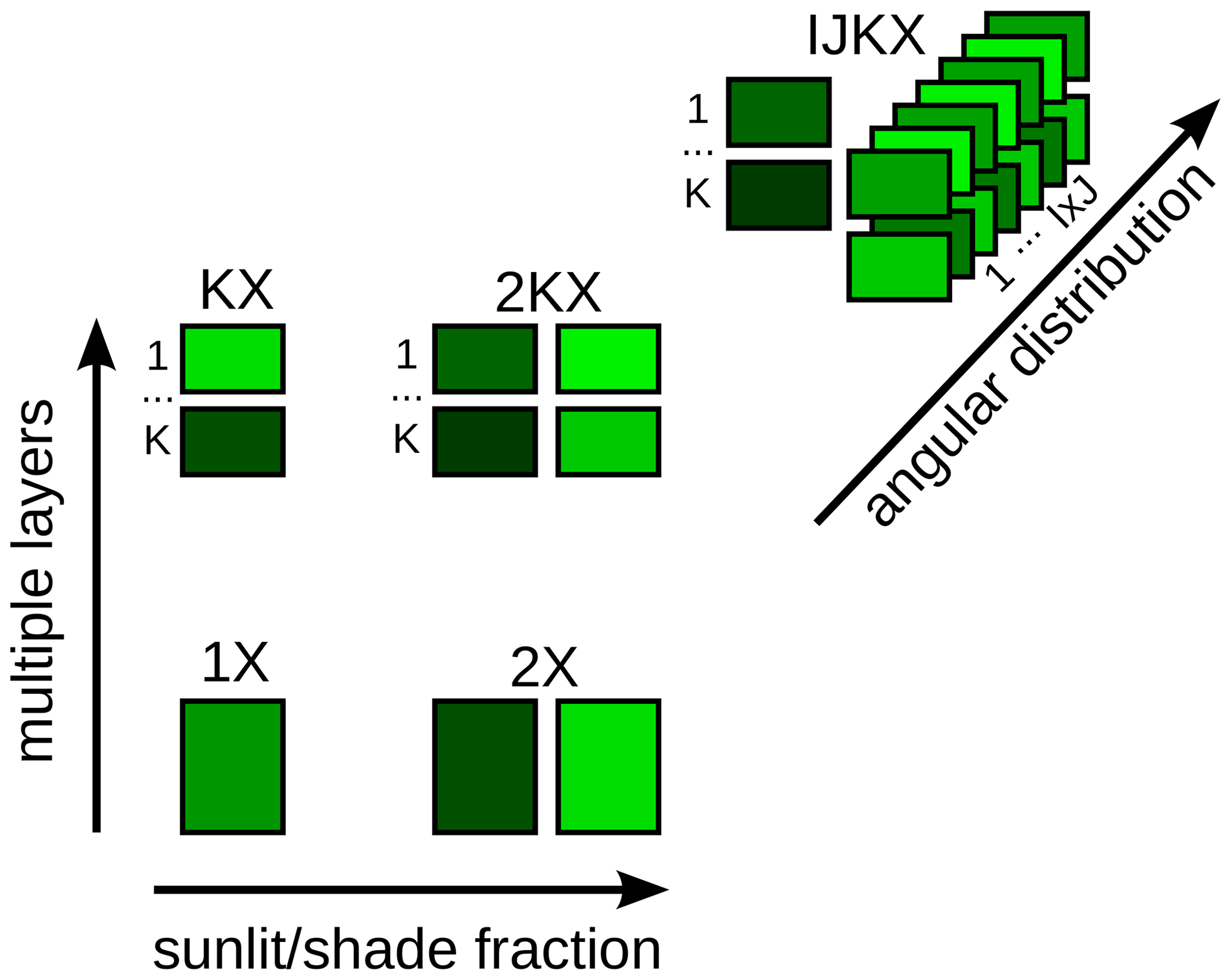
Figure 1 Canopy complexity levels. 1X: single-layer canopy without sunlit or shaded fractions. 2X: single-layer canopy with sunlit and shaded fractions. KX: multiple-layer canopy without sunlit or shaded fractions. 2KX: multiple-layer canopy with sunlit and shaded fractions per layer. IJKX: multiple-layer canopy with sunlit and shaded fractions per layer, with the sunlit fraction being further partitioned based on leaf inclination and azimuth angular distributions.

To resolve the problems of a complicated canopy, we examined by how much carbon, water, and SIF fluxes may differ when using different canopy complexity representations in the CliMA Land model, spanning from a one-layered canopy to a multi-layered canopy with hyperspectral radiation and leaf angular distributions (Fig. 1). With the model simulations, we were able to answer the following questions: (1) how does canopy complexity impact modeled canopy fluxes, and (2) could data inverted using different canopy complexity levels be compatible? Regarding the ease of understanding and using an LSM with various canopy complexities, we presented and suggested the highly modularized CliMA Land model, which can be easily set up to simulate canopy fluxes using different canopy complexity levels.

2 Materials and methods

We used the CliMA Land model (v0.1) to evaluate how canopy model complexity impacts the simulated carbon, water, and SIF fluxes. The CliMA Land model mechanistically addresses soil–plant–air continuum processes and is able to simulate canopy carbon and water fluxes as well as SIF simultaneously (Wang et al., 2021b). CliMA Land model code and documentation are freely and publicly available at https://github.com/CliMA/Land (last access: 15 November 2021).

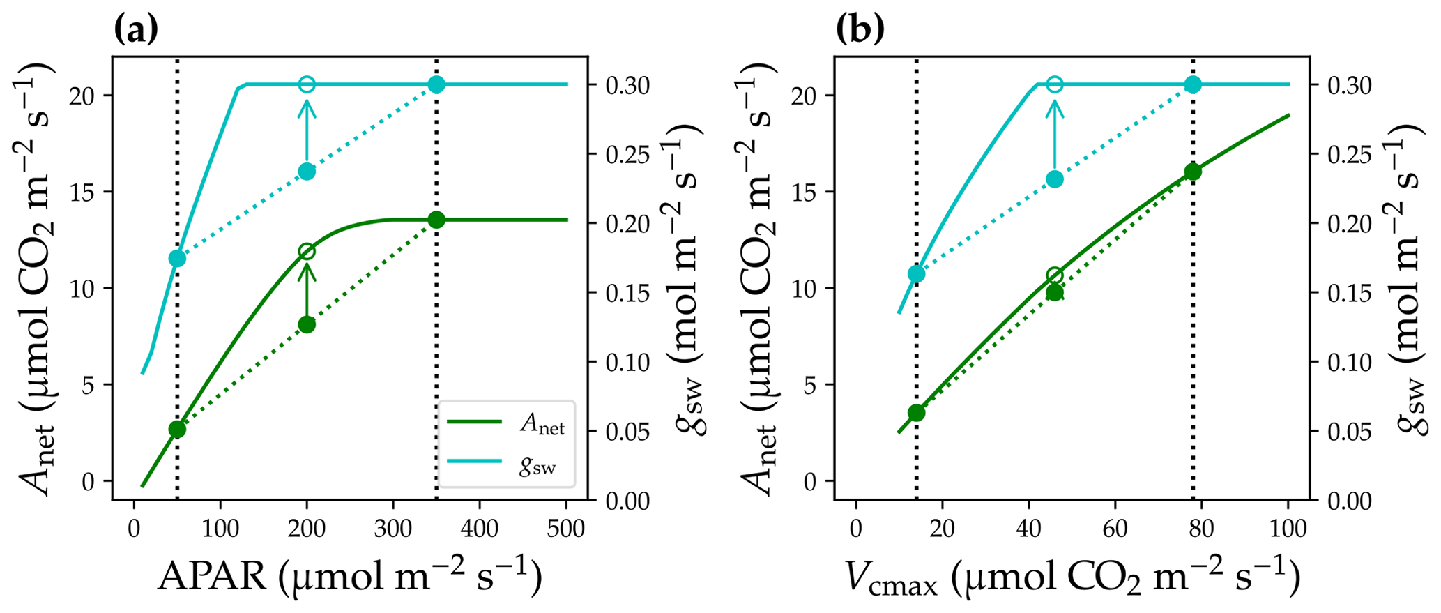
Figure 2 Non-linear leaf responses to the environmental and physiological parameters. (a) Responses of stomatal conductance to water vapor (g_sw; cyan solid curve) and net photosynthetic rate (A_net) to absorbed photosynthetically active radiation (APAR). The black dotted vertical lines indicate two leaves at low- and high-light conditions. Mean behavior of the two leaves ought to be the closed circles on the colored dotted lines. However, using mean APAR for the leaves would result in overestimated g_sw and A_net (open circles). (b) Non-linear g_sw and A_net responses to leaf photosynthetic capacity, represented by the maximum carboxylation rate (V_cmax). Environmental and leaf physiological settings for the simulations are the following: air and leaf temperatures at 298.15 K, atmospheric vapor pressure at 1500 Pa (relative humidity at 0.47), atmospheric CO₂ partial pressure at 40 Pa, atmospheric pressure at 101 325 Pa, V_cmax (for panel a) at 60 $\mathrm{\mu }\mathrm{mol}{\mathrm{m}}^{-\mathrm{2}}{\mathrm{s}}^{-\mathrm{1}}$, and maximal stomatal conductance at 0.3 $\mathrm{mol}{\mathrm{m}}^{-\mathrm{2}}{\mathrm{s}}^{-\mathrm{1}}$.

2.1 Canopy complexity levels

Leaf physiological responses to light are highly non-linear, such as stomatal conductance to water vapor (g_sw) and net photosynthetic rate (A_net). Typically, when absorbed photosynthetically active radiation (APAR) is low, g_sw and A_net increase with higher APAR (Fig. 2a); when APAR is high, g_sw and A_net saturate. If one has a leaf with low APAR and a leaf with high APAR (e.g., closed circles on the solid curves of Fig. 2a), the mean behavior of the two leaves ought to be the average g_sw and A_net values (closed circles on the colored dashed lines of Fig. 2a). However, if one uses the mean APAR of the two leaves and calculates g_sw and A_net based on the mean APAR, g_sw and A_net would be overestimated (open circles on the colored solid curves of Fig. 2a). Note that averaging APAR values that are beyond the turning point, say 350 $\mathrm{\mu }\mathrm{mol}{\mathrm{m}}^{-\mathrm{2}}{\mathrm{s}}^{-\mathrm{1}}$, may not result in any bias in modeled g_sw and A_net (such as for sunlit and shaded leaves in the top canopy layer); however, averaging APAR for leaves with high APAR and low APAR, say 300 and 50 $\mathrm{\mu }\mathrm{mol}{\mathrm{m}}^{-\mathrm{2}}{\mathrm{s}}^{-\mathrm{1}}$, would result in overestimated g_sw and A_net (such as for shaded leaves in an upper and lower canopy as typically done in the two-leaf radiation scheme). Thus, an overly simplified canopy model may overestimate canopy-level carbon and water fluxes, because of the inappropriately averaged APAR, as $f\left(\stackrel{\mathrm{‾}}{x}\right)\ne \stackrel{\mathrm{‾}}{f\left(x\right)}$ when averaging non-linear functions ($A_{\text{net}}\left(\stackrel{\mathrm{‾}}{\text{APAR}}\right)>\stackrel{\mathrm{‾}}{A_{\text{net}}\left(\text{APAR}\right)}$ in leaf photosynthesis).

Bonan et al. (2011)Lawrence et al. (2019)Bonan et al. (2018)Carrer et al. (2013)Boone et al. (2017)Jogireddy et al. (2006)Clark et al. (2011)Clark et al. (2011)Ryder et al. (2016)van der Tol et al. (2009)Yang et al. (2021)Yang et al. (2021)

Table 1 A list of vegetation models corresponding to our tested canopy complexity schemes. CLM: Community Land Model. ISBA: Interactions between soil–biosphere–atmosphere. JULES: Joint UK Land Environment Simulator. ORCHIDEE: Organising Carbon and Hydrology In Dynamic Ecosystems. SCOPE: Soil Canopy Observation, Photochemistry and Energy fluxes. 2X: single-layer canopy with sunlit and shaded fractions. KX: multiple-layer canopy without sunlit or shaded fractions. 2KX: multiple-layer canopy with sunlit and shaded fractions per layer. IJKX: multiple-layer canopy with sunlit and shaded fractions per layer, with the sunlit fraction being further partitioned based on leaf inclination and azimuth angular distributions.

To evaluate how much canopy model complexity matters, we modeled the canopy using five different levels of complexity, and they are denoted as “1X”, “2X”, “KX”, “2KX”, and “IJKX” (Fig. 1). 1X represents the scenario in which the canopy is treated as a single average leaf without sunlit or shaded fractions, and leaf radiation is averaged for the entire canopy. 2X complicates 1X by partitioning the average leaf to sunlit and shaded fractions. KX enhances 1X by partitioning the canopy to multiple layers (but no sunlit or shaded fractions per layer). 2KX partitions each canopy layer of KX to sunlit and shaded fractions. IJKX further modifies 2KX by accounting for leaf inclination and azimuth angle distributions per layer (Fig. 1). See Table 1 for the canopy model complexity adopted by other vegetation models (see https://yujie-w.github.io/PAGES/dev/methods/#Vegetation-canopy-model-complexity for a growing list).

For IJKX, we simulated the canopy radiative transfer using the CliMA Land-adapted SCOPE model (Soil Canopy Observation, Photochemistry and Energy fluxes; SCOPE v1.7; Yang et al., 2017). The adaptations included that carotenoid absorption was accounted for as APAR (Wang et al., 2021b) and that canopy clumping was addressed using a clumping index (Braghiere et al., 2021). At layer i, the shaded-leaf fraction (relative to total leaf area in the canopy) is p_sh,i, and the sunlit-leaf fraction (relative to total leaf area in the canopy) is p_sl,i(incl, azi) (“incl” is the inclination angle, and “azi” is the azimuth angle). The fraction of sunlit leaves relative to total canopy leaf area in a given canopy layer is computed as

$$\begin{array}{}\text{(1)}& \begin{array}{rl}\sum _{\text{incl,azi}}{p}_{\text{sl},i}\left(\text{incl,azi}\right)=& {\displaystyle \frac{\text{LAI}(i+\mathrm{1})-\text{LAI}\left(i\right)}{\text{LAI }}}\\ & \cdot \underset{\text{LAI}\left(i\right)}{\overset{\text{LAI}(i+\mathrm{1})}{\int }}\exp (-k\mathrm{\Omega }x)\cdot \mathrm{d}x,\end{array}\end{array}$$

where LAI is total leaf area index, LAI(i) is the leaf area index above the ith canopy layer, LAI(i+1) is the leaf area index in and above the ith canopy layer, k is the extinction coefficient as a function of leaf inclination angle distribution, and Ω is the clumping index. Then p_sl,i(incl,azi) is computed using

$$\begin{array}{}\text{(2)}& p_{\text{sl},i}\left(\text{incl,azi}\right)=\sum _{\text{incl,azi}}{p}_{\text{sl},i}\left(\text{incl,azi}\right)\cdot {\displaystyle \frac{\mathrm{1}}{I}}\cdot {\displaystyle \frac{\mathrm{1}}{J}},\end{array}$$

where I is the number of inclination angles and J is the number of azimuth angles. The fraction of shaded leaves relative to total canopy leaf area in a given canopy layer is computed as

$$\begin{array}{}\text{(3)}& \begin{array}{rl}{p}_{\text{sh},i}=& {\displaystyle \frac{\text{LAI}(i+\mathrm{1})-\text{LAI}\left(i\right)}{\text{LAI}}}\\ & \cdot \left[\mathrm{1}-\underset{\text{LAI}\left(i\right)}{\overset{\text{LAI}(i+\mathrm{1})}{\int }}\exp (-k\mathrm{\Omega }x)\cdot \mathrm{d}x\right].\end{array}\end{array}$$

Corresponding APAR values for the shaded and sunlit leaves are APAR_sh and APAR_sl,i(incl, azi), respectively. We used default values of I = 9 inclination angles, J = 36 azimuth angles, and K = 20 vertical layers for IJKX (K = 20 for 2KX and KX as well).

The 2KX fraction and APAR were derived from IJKX by weighing APAR for sunlit leaves per canopy layer:

$$\begin{array}{}\text{(4)}& \begin{array}{rl}& {}^{\text{2KX}}{p}_{\text{sl},i}=\sum _{\text{incl,azi}}{p}_{\text{sl},i}\left(\text{incl,azi}\right),\\ & {}^{\text{2KX}}{p}_{\text{sh},i}=p_{\text{sh},i},\\ & {}^{\text{2KX}}{\text{APAR}}_{\text{sl},i}={\displaystyle \frac{{\sum }_{\text{incl,azi}}\left[{\text{APAR}}_{\text{sl},i}\left(\text{incl,azi}\right)\cdot p_{\text{sl},i}\left(\text{incl,azi}\right)\right]}{{\sum }_{\text{incl,azi}}\left[p_{\text{sl},i}\left(\text{incl,azi}\right)\right]}},\\ & {}^{\text{2KX}}{\text{APAR}}_{\text{sh},i}={\text{APAR}}_{\text{sh},i}.\end{array}\end{array}$$

The KX fraction and APAR were derived from 2KX by weighing APAR for all sunlit and shaded leaves per canopy layer:

$$\begin{array}{}\text{(5)}& \begin{array}{r}{}^{\text{KX}}{p}_i={}^{\text{2KX}}{p}_{\text{sl},i}+{}^{\text{2KX}}{p}_{\text{sh},i},\\ {}^{\text{KX}}{\text{APAR}}_i={\displaystyle \frac{{}^{\text{2KX}}{\text{APAR}}_{\text{sl},i}{\cdot }^{\text{2KX}}{p}_{\text{sl},i}+{}^{\text{2KX}}{\text{APAR}}_{\text{sh},i}{\cdot }^{\text{2KX}}{p}_{\text{sh},i}}{{}^{\text{KX}}{p}_i}}.\end{array}\end{array}$$

The 2X fraction and APAR were derived from 2KX by weighing APAR for sunlit and shaded leaves for all canopy layers, respectively, the following:

$$\begin{array}{}\text{(6)}& \begin{array}{rl}& {}^{\text{2X}}{p}_{\text{sl}}=\sum _i{p}_{\text{sl},i},\\ & {}^{\text{2X}}{p}_{\text{sh}}=\sum _i{p}_{\text{sh},i},\\ & {}^{\text{2X}}{\text{APAR}}_{\text{sl}}={\displaystyle \frac{{\sum }_i\left({}^{\text{2KX}}{\text{APAR}}_{\text{sl},i}{\cdot }^{\text{2KX}}{p}_{\text{sl},i}\right)}{{\sum }_i\left({}^{\text{2KX}}{p}_{\text{sl},i}\right)}},\\ & {}^{\text{2X}}{\text{APAR}}_{\text{sh}}={\displaystyle \frac{{\sum }_i\left({}^{\text{2KX}}{\text{APAR}}_{\text{sh},i}{\cdot }^{\text{2KX}}{p}_{\text{sh},i}\right)}{{\sum }_i\left({}^{\text{2KX}}{p}_{\text{sh},i}\right)}}.\end{array}\end{array}$$

1X APAR was derived from KX by weighing APAR for all layers:

$$\begin{array}{}\text{(7)}& {}^{\text{1X}}\text{APAR}=\sum _i\left({}^{\text{KX}}{\text{APAR}}_i{\cdot }^{\text{KX}}{p}_i\right).\end{array}$$

Figure 3 Comparison of profiles of mean absorbed photosynthetically active radiation (APAR) for four different canopy complexity levels. 1X: single-layer canopy without sunlit or shaded fractions. 2X: single-layer canopy with sunlit and shaded fractions. KX: multiple-layer canopy without sunlit or shaded fractions. 2KX: multiple-layer canopy with sunlit and shaded fractions per layer. IJKX: multiple-layer canopy with sunlit and shade fractions per layer, with the sunlit fraction being further partitioned based on leaf inclination and azimuth angular distributions. The abbreviations “sl” and “sh” stand for sunlit and shaded leaves, respectively.

We emphasize here that to derive canopy fluorescence spectrum and its sun-sensor geometry, we need to simulate the canopy radiative transfer using hyperspectral reflectance, transmittance, and fluorescence. Due to the high spectral resolution and multiple layers required, radiative transfer and canopy fractions in complex models such as SCOPE are computed numerically. In comparison, radiative transfer and sunlit/shaded fractions are computed analytically in the two-leaf radiation scheme, as the model is single layered and uses broadband reflectance and transmittance (Campbell and Norman, 1998; Bonan et al., 2021). Yet, the two-leaf radiation schemes that use broadband radiative transfer are not adequate for accurate fluorescence modeling. Crucially, the difference in the analytic and numerical solutions could result in biases in the simulated APAR and fraction. To avoid such bias, we computed APAR and sunlit/shaded fractions for the simpler canopy setups numerically using the algorithm in IJKX. See Fig. 3 for the APAR profiles for 2KX, KX, 2X, and 1X derived from IJKX. Also, we note here that leaf biochemical parameters and APAR were not integrated within a canopy layer or sunlit/shaded fractions; instead, we used average APAR and leaf traits in our simulations. Thus, our 1X model is a one-leaf model rather than a one-big-leaf model, and our 2X model resembles the two-leaf model rather than the two-big-leaf model.

2.2 Vertical canopy profile

Leaf traits in the canopy are not uniform among the canopy layers. Typically, leaf photosynthetic capacity (usually represented by the maximum carboxylation rate at 25 ^∘C, V_cmax) is higher in upper canopy because of the better light environment. Further, leaf physiological responses to V_cmax are also highly non-linear, and using average V_cmax may also result in overestimated g_sw and A_net and thus carbon and water fluxes (e.g., shift from solid circles to open circles in Fig. 2b).

To examine how much the vertical V_cmax profile impacts modeled canopy flux simulations, we ran the model simulation in two scenarios, one using uniform V_cmax in the canopy and one using decreasing V_cmax towards the lower canopy. For the latter scenario, V_cmax at layer i was tuned using an exponential function following De Pury and Farquhar (1997) and Chen et al. (2012):

$$\begin{array}{}\text{(8)}& V_{\text{cmax},i}=V_{\text{cmax,top}}\cdot \exp \left[-\mathrm{0.15}\cdot \text{LAI}\left(i\right)\right],\end{array}$$

where V_cmax,top is V_cmax at the top of the canopy and 0.15 is the shape factor that describes the decreasing V_cmax with canopy depth. Note that as leaves are experiencing dynamically changing light environment throughout the day, it is unrealistic to assume the sunlit and shaded leaves have different traits; thus, we only accounted for the vertical heterogeneity but neglected the horizontal heterogeneity in each canopy layer, namely using the same characteristics for leaves within the same canopy layer.

The V_cmax profile was applied to IJKX, 2KX, and KX directly, whereas weighed mean $V_{\text{cmax}}={\sum }_i{V}_{\text{cmax},i}{\cdot }^{\text{KX}}{p}_i$ was used in 1X. The V_cmax profile or value stayed constant in these four scenarios throughout the simulation, as sunlit/shaded fractions did not impact them. We note here that mean V_cmax changed with sunlit/shaded fractions in 2X (Chen et al., 2012) and particular averages of V_cmax for sunlit and shaded fractions (^2XV_cmax,sl and ^2XV_cmax,sh, respectively) need to be updated with sunlit and shaded fractions:

$$\begin{array}{}\text{(9)}& \begin{array}{r}{}^{\text{2X}}{V}_{\text{cmax,sl}}={\displaystyle \frac{{\sum }_i\left({}^{\text{2KX}}{V}_{\text{cmax},i}{\cdot }^{\text{2KX}}{p}_{\text{sl},i}\right)}{{\sum }_i\left({}^{\text{2KX}}{p}_{\text{sl},i}\right)}},\\ {}^{\text{2X}}{V}_{\text{cmax,sh}}={\displaystyle \frac{{\sum }_i\left({}^{\text{2KX}}{V}_{\text{cmax},i}{\cdot }^{\text{2KX}}{p}_{\text{sh},i}\right)}{{\sum }_i\left({}^{\text{2KX}}{p}_{\text{sh},i}\right)}}.\end{array}\end{array}$$

Note that we tuned the maximum electron transport rate and leaf respiration rate in the same manner as V_cmax.

2.3 Canopy flux simulations

We simulated the canopy carbon and water fluxes using a stomatal optimization model developed in Wang et al. (2020) given the good model performance and scalability (Wang et al., 2021a). The stomatal optimization model posits that stomatal opening is optimized when the difference between carbon gain and risk is maximum:

$$\begin{array}{}\text{(10)}& max\underset{\text{gain}}{\underbrace{A_{\text{net}}}}-\underset{\text{risk}}{\underbrace{A_{\text{net}}\cdot {\displaystyle \frac{E}{E_{\text{crit}}}}}},\end{array}$$

where E is the leaf transpiration rate and E_crit is the critical transpiration rate of the leaf beyond which leaf hydraulic conductance drops below 0.1 % of the maximum (see Sperry et al., 2016, and Wang et al., 2021b, for more details of E_crit).

At each canopy complexity level, for a given environmental condition set, we were able to obtain the steady-state stomatal conductance for each APAR, from which we computed steady-state A_net using the classic C3 photosynthesis model (Farquhar et al., 1980) and E as well as leaf fluorescence quantum yield (ϕ_F) using the model developed in van der Tol et al. (2014). Stand-level carbon flux, namely net ecosystem exchange (NEE; normalized per ground area), was computed using $\text{NEE}=\text{LAI}\cdot \sum \left(A_{\text{net}}\cdot p\right)-R_{\text{remain}}$:

$$\begin{array}{}\text{(11)}& \begin{array}{rl}{}^{\text{IJKX}}\text{NEE}=& \text{LAI}\cdot \sum _{\text{i,incl,azi}}\left[A_{\text{net}}\left({\text{APAR}}_{\text{sl},i}\left(\text{incl,azi}\right)\right)\right.\\ & \left.\cdot p_{\text{sl},i}\left(\text{incl,azi}\right)\right]+\text{LAI}\cdot \sum _i\left[A_{\text{net}}\left({\text{APAR}}_{\text{sh},i}\right)\right.\\ & \left.\cdot p_{\text{sh},i}\right]-R_{\text{remain}},\\ {}^{\text{2KX}}\text{NEE}=& \text{LAI}\cdot \sum _i\left[A_{\text{net}}\left({}^{\text{2KX}}{\text{APAR}}_{\text{sl},i}\right){\cdot }^{\text{2KX}}{p}_{\text{sl},i}\right.\\ & \left.+A_{\text{net}}\left({}^{\text{2KX}}{\text{APAR}}_{\text{sh},i}\right){\cdot }^{\text{2KX}}{p}_{\text{sh},i}\right]-R_{\text{remain}},\\ {}^{\text{KX}}\text{NEE}=& \text{LAI}\cdot \sum _i\left[A_{\text{net}}\left({}^{\text{KX}}\text{APAR}\right){\cdot }^{\text{KX}}{p}_i\right]-R_{\text{remain}},\\ {}^{\text{2X}}\text{NEE}=& \text{LAI}\cdot A_{\text{net}}\left({}^{\text{2X}}{\text{APAR}}_{\text{sl}}\right){\cdot }^{\text{2X}}{p}_{\text{sl}}\\ & +\text{LAI}\cdot A_{\text{net}}\left({}^{\text{2X}}{\text{APAR}}_{\text{sh}}\right){\cdot }^{\text{2X}}{p}_{\text{sh}}-R_{\text{remain}},\\ {}^{\text{1X}}\text{NEE}=& \text{LAI}\cdot A_{\text{net}}\left({}^{\text{1X}}\text{APAR}\right)-R_{\text{remain}},\end{array}\end{array}$$

where LAI is the leaf area index and R_remain is the ecosystem respiration rate per ground area excluding the leaves. The transpiration rate from the canopy is computed and used as a proxy for estimating the difference in model ecosystem evapotranspiration (ET; normalized per ground area) using $\text{ET}\approx \text{LAI}\cdot \sum (E\cdot p)$:

$$\begin{array}{}\text{(12)}& \begin{array}{rl}{}^{\text{IJKX}}\text{ET}\approx & \text{LAI}\cdot \sum _{\text{i,incl,azi}}\left[E\left({\text{APAR}}_{\text{sl},i}\left(\text{incl,azi}\right)\right)\right.\\ & \left.\cdot p_{\text{sl},i}\left(\text{incl,azi}\right)\right]+\text{LAI}\cdot \sum _i\left[E\left({\text{APAR}}_{\text{sh},i}\right)\cdot p_{\text{sh},i}\right],\\ {}^{\text{2KX}}\text{ET}\approx & \text{LAI}\cdot \sum _i\left[E\left({}^{\text{2KX}}{\text{APAR}}_{\text{sl},i}\right){\cdot }^{\text{2KX}}{p}_{\text{sl},i}\right.\\ & \left.+E\left({}^{\text{2KX}}{\text{APAR}}_{\text{sh},i}\right){\cdot }^{\text{2KX}}{p}_{\text{sh},i}\right],\\ {}^{\text{KX}}\text{ET}\approx & \text{LAI}\cdot \sum _i\left[E\left({}^{\text{KX}}\text{APAR}\right){\cdot }^{\text{KX}}{p}_i\right],\\ {}^{\text{2X}}\text{ET}\approx & \text{LAI}\cdot E\left({}^{\text{2X}}{\text{APAR}}_{\text{sl}}\right){\cdot }^{\text{2X}}{p}_{\text{sl}}\\ & +\text{LAI}\cdot E\left({}^{\text{2X}}{\text{APAR}}_{\text{sh}}\right){\cdot }^{\text{2X}}{p}_{\text{sh}},\\ {}^{\text{1X}}\text{ET}\approx & \text{LAI}\cdot E\left({}^{\text{1X}}\text{APAR}\right).\end{array}\end{array}$$

We remind the reader here that soil evaporation is a function of soil water content, soil surface temperature, and atmospheric-vapor-pressure deficit and that soil evaporation should be the same for all tested canopy complexity models; this is also the case for evaporation from intercepted water on plant surface. Therefore, the modeled ET difference is 100 % caused by canopy transpiration, and using transpiration would not result in any biases in the relative difference of modeled ET.

For IJKX, we used ϕ_F computed for each sunlit and shaded leaf at each layer to compute the canopy-level SIF spectrum. For 2KX, we plugged the ϕ_F calculated for sunlit fraction into all the sunlit leaves of the corresponding layer of IJKX and the shaded ϕ_F into the shaded leaf of the corresponding layer of IJKX. Then we re-simulated the SIF spectrum at IJKX and used it as that of 2KX. For KX, we plugged the ϕ_F calculated for the whole layer into all the leaves of the corresponding layer of IJKX and recalculated the SIF spectrum. For 2X, we plugged the ϕ_F of the sunlit fraction into all the sunlit leaves in IJKX and shaded ϕ_F into all the shaded leaves in IJKX and recalculated the SIF spectrum. For 1X, we plugged the ϕ_F into all the leaves in IJKX and recalculated the SIF spectrum. We compared SIF at 740 nm (SIF₇₄₀) among different complexity levels.

Despite the importance of vertical microclimate heterogeneity in modeled canopy energy fluxes (e.g., Bonan et al., 2021), we held environmental conditions constant among vertical canopy layers for all tested canopy complexities. Doing this allowed us to tease apart the impact of APAR distribution in the canopy (due to canopy complexity) on simulated carbon, water, and SIF fluxes.

2.4 Sensitivity analysis

We ran a sensitivity analysis to environmental cues for all five complexity levels to examine how much they differ in predicted carbon, water, and SIF fluxes. The tested cues included solar radiation, atmospheric-vapor-pressure deficit (VPD), temperature, soil water potential (Ψ_soil), and atmospheric CO₂ partial pressure ($P_{{\mathrm{CO}}_{\mathrm{2}}}$). When we altered temperature, we changed the air and leaf temperature at the same time and held air relative humidity (RH) constant at 0.47 (fraction; unitless). Saturated water vapor pressure was computed using the Clausius–Clapeyron equation:

$$\begin{array}{}\text{(13)}& \begin{array}{rl}{P}_{\text{sat}}=& P_{\text{triple}}\cdot {\left({\displaystyle \frac{T}{T_{\text{triple}}}}\right)}^{\frac{\mathrm{\Delta }{c}_{\text{p}}}{R_{\text{v}}}}\\ & \cdot \exp \left[{\displaystyle \frac{{\text{LH}}_{\text{v0}}-\mathrm{\Delta }{c}_{\text{p}}\cdot T_{\text{triple}}}{R_{\text{v}}}}\cdot \left({\displaystyle \frac{\mathrm{1}}{T_{\text{triple}}}}-{\displaystyle \frac{\mathrm{1}}{T}}\right)\right],\end{array}\end{array}$$

where P_triple is the vapor pressure at the triple point (in Pa), T is the temperature (in K), T_triple is the temperature at the triple point (in K), Δc_p is the difference in isobaric specific heat of vapor and liquid (in $\mathrm{J}{\mathrm{Kg}}^{-\mathrm{1}}{\mathrm{K}}^{-\mathrm{1}}$), R_v is the gas constant of water vapor (in $\mathrm{J}{\mathrm{Kg}}^{-\mathrm{1}}{\mathrm{K}}^{-\mathrm{1}}$), and LH_v0 is the latent heat of vaporization at the triple point. Atmospheric vapor pressure was computed using P_sat⋅RH. For each tested environmental cue, we changed only the tested cue while holding all other environmental conditions constant. We ran the sensitivity test in two scenarios: (a) V_cmax was uniform throughout the canopy, and (b) V_cmax decreased exponentially in the lower canopy. For the two scenarios, we let the entire-canopy mean V_cmax be the same (namely mean V_cmax at 1X). We compared the modeled site-level NEE, ET, and SIF₇₄₀ among canopy complexity levels.

2.5 Diurnal cycles

To evaluate how much the canopy complexity models differ in real-world simulations, we ran the model using weather data from a flux tower located at Ozark, Missouri, USA (US-MOz; Gu et al., 2016). We used the weather and soil moisture data from day 177 to 179 in the year 2019 and prescribed leaf temperature and soil water potential to maximally reduce uncertainty among model setups. Briefly, we used outgoing longwave radiation from flux tower measurements to invert canopy temperature and used it as leaf temperature; we also used soil water content to estimate soil water potential and used it as a boundary condition for the soil–plant–air continuum. Prescribing leaf temperature and soil water potential allowed us to tease apart the difference caused by canopy complexity from that caused by environmental and physiological differences. See Wang et al. (2021b) for the model setup details for US-MOz. In addition to the observations that were used to set up the CliMA Land model (Wang et al., 2021b), we further applied vertical V_cmax profiles in the simulations (note that V_cmax changed in the sunlit and shaded fractions with time for 2X and stayed constant for the other four complexity levels). We tuned V_cmax and the whole-plant hydraulic conductance to let IJKX predict reasonable NEE and ET values and used these tuned parameters in all the tested canopy complexity levels. We note here that we were not trying to argue one complexity was better than others but to examine how much the complexity levels differ when we used exactly the same model input parameters.

We compared the model-predicted carbon, water, and SIF fluxes. Note here that observed SIF depends on the sun-sensor geometry and that SIF retrievals often have different sun-sensor geometries (e.g., the TROPOMI satellite; Köhler et al., 2018). Thus, it is necessary to examine how the sun-sensor geometry may impact the SIF flux across canopy complexity levels. We ran the test using the weather data from (a) 12:00–12:30 and (b) 16:00–16:30 of day 177 in the year 2019. At each tested time window, we computed the theoretical SIF at 740 nm for a series of viewing zenith angles from 0 to 85^∘ and relative azimuth angles (angle between the sensor and sun) from 0 to 360^∘. We compared how much 2KX, KX, 2X, and 1X differed from IJKX.

Given that averaging APAR theoretically results in overestimated carbon and water fluxes, we expected that the difference among different canopy complexity levels meets the following trends: (a) 1X > 2X > 2KX and (b) 1X > KX > 2KX. Further, as V_cmax also theoretically results in overestimated carbon and water fluxes, we expected that adding a vertical V_cmax profile further increases the difference in fluxes across canopy complexity levels.

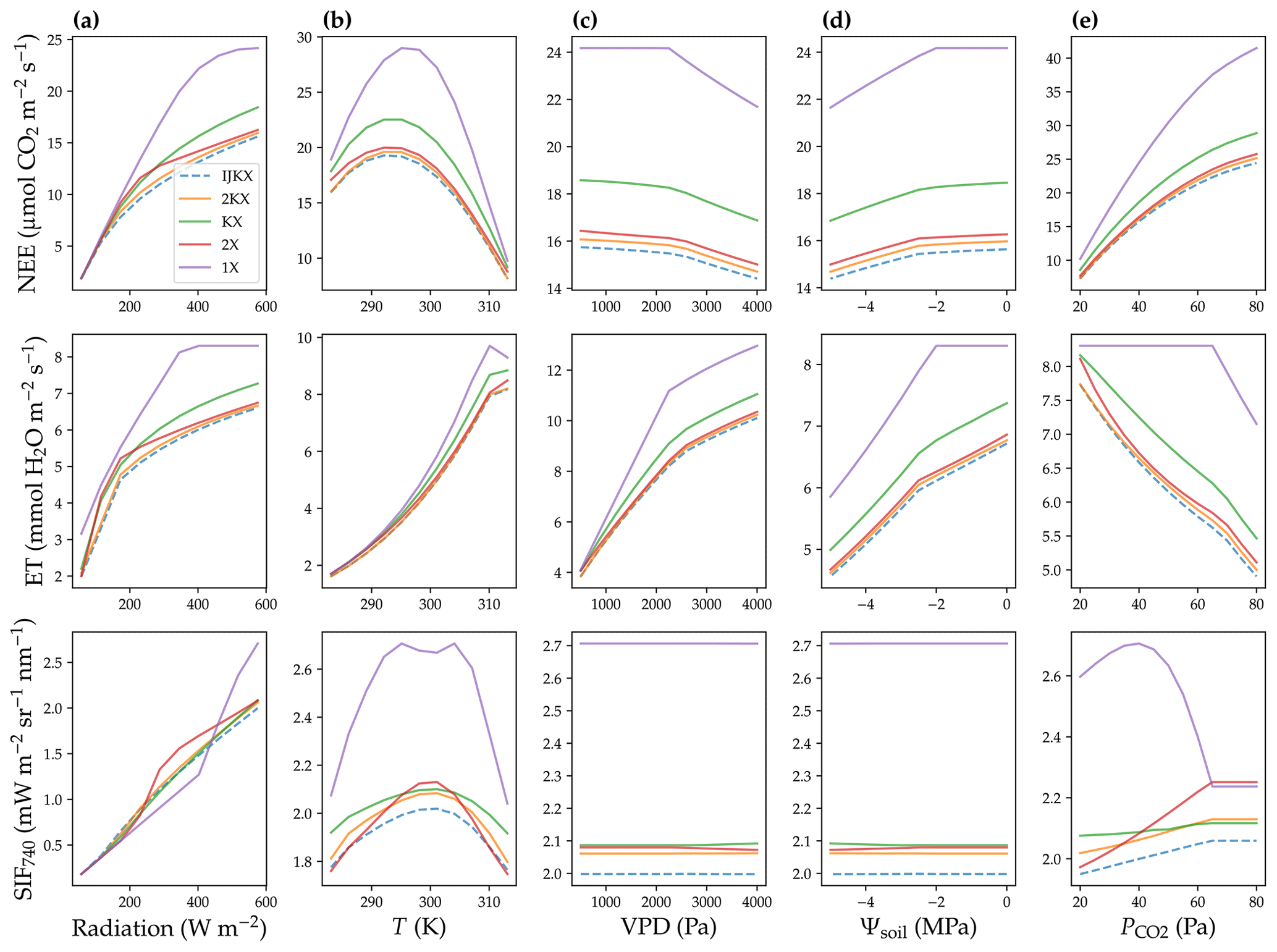
Figure 4 Net ecosystem exchange of CO₂ (NEE, normalized per ground area), evapotranspiration rate (ET, normalized per ground area), and solar-induced fluorescence (SIF) responses to changes in environmental cues. (a) Responses to total radiation. (b) Responses to air and leaf temperature (T). (c) Responses to atmospheric-vapor-pressure deficit (VPD). (d) Responses to soil water potential (Ψ_soil). (e) Responses to atmospheric CO₂ partial pressure ($P_{{\mathrm{CO}}_{\mathrm{2}}}$). This sensitivity analysis was done assuming uniform photosynthetic capacity in the canopy.

3 Results

3.1 Sensitivity analysis

When a uniform V_cmax profile was applied, all tested five canopy complexity levels exhibited similar carbon and water flux responses to changing environmental cues (Fig. 4). The responses included increasing canopy photosynthesis and transpiration with higher radiation (Fig. 4a), increasing and then decreasing photosynthesis and increasing transpiration with a higher temperature (Fig. 4b), decreasing photosynthesis and increasing transpiration with a higher VPD (Fig. 4c), decreasing photosynthesis and transpiration with drier soil (Fig. 4d), and increasing photosynthesis and decreasing transpiration with higher atmospheric CO₂ partial pressure (Fig. 4e). Further, as expected, 1X, 2X, KX, and 2KX all overestimated canopy photosynthesis and transpiration compared to the IJKX mode; and the overestimation ratios met 1X > 2X > 2KX and 1X > KX > 2KX.

The SIF responses to changing environmental cues in general agreed in trends among tested complexity levels (Fig. 4). However, SIF responses to radiation, temperature, and atmospheric CO₂ differed dramatically among the five canopy complexity levels given the different response magnitudes (Fig. 4b and e). 1X and KX often resulted in different trends compared to IJKX (Fig. 4). 2X and 2KX overall tracked the SIF responses though slightly overestimated SIF of IJKX well. Notably, we found high disagreement between 2X and IJKX at intermediate radiation and increasing disagreement at higher atmospheric CO₂ (Fig. 4a and e).

Figure 5 Net ecosystem exchange of CO₂ (NEE, normalized per ground area), evapotranspiration rate (ET, normalized per ground area), and solar-induced fluorescence (SIF) responses to changes in environmental cues. (a) Responses to total radiation. (b) Responses to air and leaf temperature (T). (c) Responses to atmospheric-vapor-pressure deficit (VPD). (d) Responses to soil water potential (Ψ_soil). (e) Responses to atmospheric CO₂ partial pressure ($P_{{\mathrm{CO}}_{\mathrm{2}}}$). This sensitivity analysis was done assuming exponentially decreasing photosynthetic capacity in the lower canopy.

When an exponential vertical V_cmax profile (lower V_cmax in the lower canopy) was applied when simulating canopy fluxes, we found similar trends compared to the scenario with constant V_cmax (Fig. 5). The differences, however, were that all carbon, water, and SIF fluxes were lower when we applied a vertical V_cmax profile (Fig. 5). Again, like the scenario of a uniform V_cmax, we also found divergent SIF responses to radiation and increasing disagreements among 2X, 2KX, and IJKX for elevated CO₂ (Fig. 5a and e). The divergent flux responses to $P_{{\mathrm{CO}}_{\mathrm{2}}}$ underlined the importance of adopting a more complex canopy in future land modeling given that (i) CO₂ concentration within the canopy airspace may change dramatically within a diurnal cycle due to plant carbon fixation and (ii) atmospheric mean CO₂ is increasing rapidly due to anthropogenic emissions.

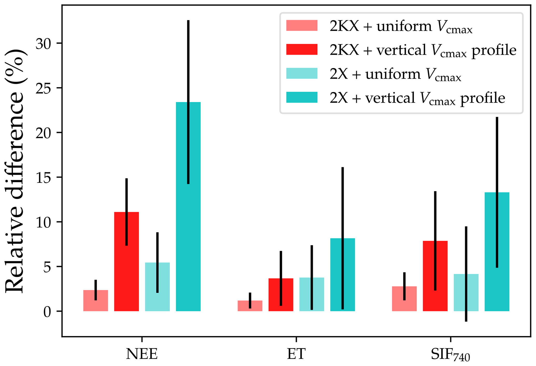
Figure 6 Relative differences between IJKX, 2KX, and 2X for the net ecosystem exchange of CO₂ (NEE), evapotranspiration (ET), and solar-induced chlorophyll fluorescence (SIF₇₄₀) fluxes. The lighter bars indicate the case with uniform leaf photosynthetic capacity in the canopy. The darker bars indicate the case with a profile of vertical photosynthetic capacity (exponentially decreasing capacity in the lower canopy). The bars plot relative differences of the fluxes compared to IJKX (positive value means overestimated flux).

2KX and 2X had a lower difference from IJKX compared to KX and 1X, and 2KX had the lowest error given the better-resolved APAR fractions (Figs. 4 and 5). Combining all response curves together from Fig. 4, we found that when V_cmax was evenly distributed in the canopy, relative differences between 2KX and IJKX for carbon, water, and SIF fluxes were 2.4 %, 1.2 %, and 2.8 %, respectively (Fig. 6). In comparison, the differences between 2X and IJKX were all higher at 5.4 %, 3.8 %, and 4.2 %, respectively (Fig. 6). Overall, 2KX had a relative error lower than 5 % (Fig. 6).

When accounting for a vertically heterogeneous V_cmax profile, we still found a lower difference between 2KX and IJKX, and the relative differences were 11.1 %, 3.7 %, and 7.9 % (the differences for 2X were 23.4 %, 8.2 %, and 13.2 %; Fig. 6). Overall, 2KX had a relative error lower than 10 %. Further, the higher error when adopting a vertical V_cmax profile agreed with our expectation as the impacts from APAR and V_cmax added up (canopy fluorescence was lower for the simpler canopy model at low radiations; Fig. 6).

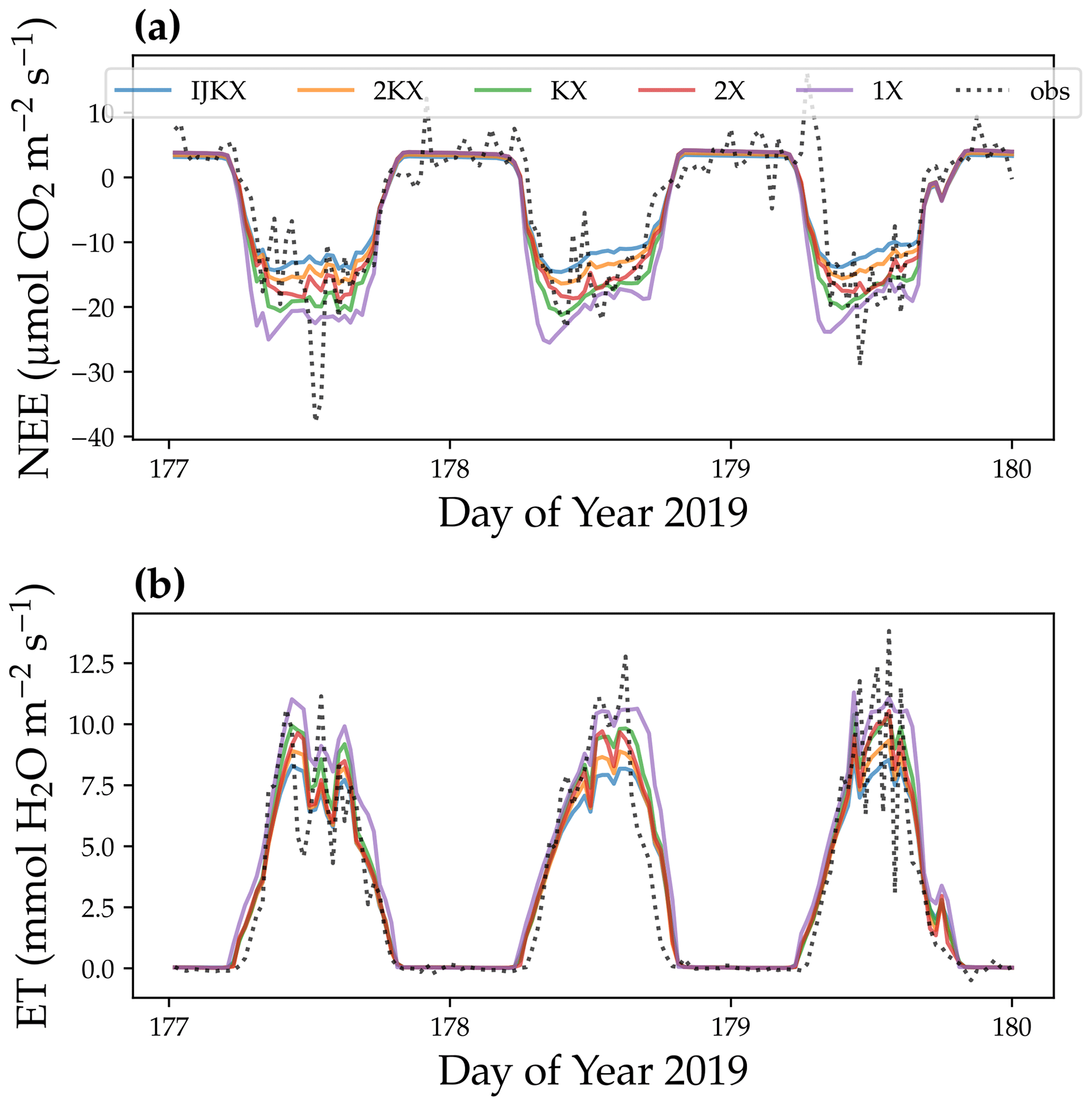
Figure 7 Diurnal cycle of carbon and water fluxes using five different canopy complexity levels. (a) Site-level net ecosystem exchange of CO₂ (NEE). (b) Site-level evaporation transpiration using plant transpiration as a proxy (ET). The dotted lines were observations from a flux tower at Ozark, Missouri, USA (US-MOz). The colored lines were model simulations with a profile of vertical leaf photosynthetic capacity using observed weather drivers from day 177 to 179 in the year 2019, such as air and soil humidity. For NEE, a more negative value means higher carbon flux; for ET, a higher value means higher water flux.

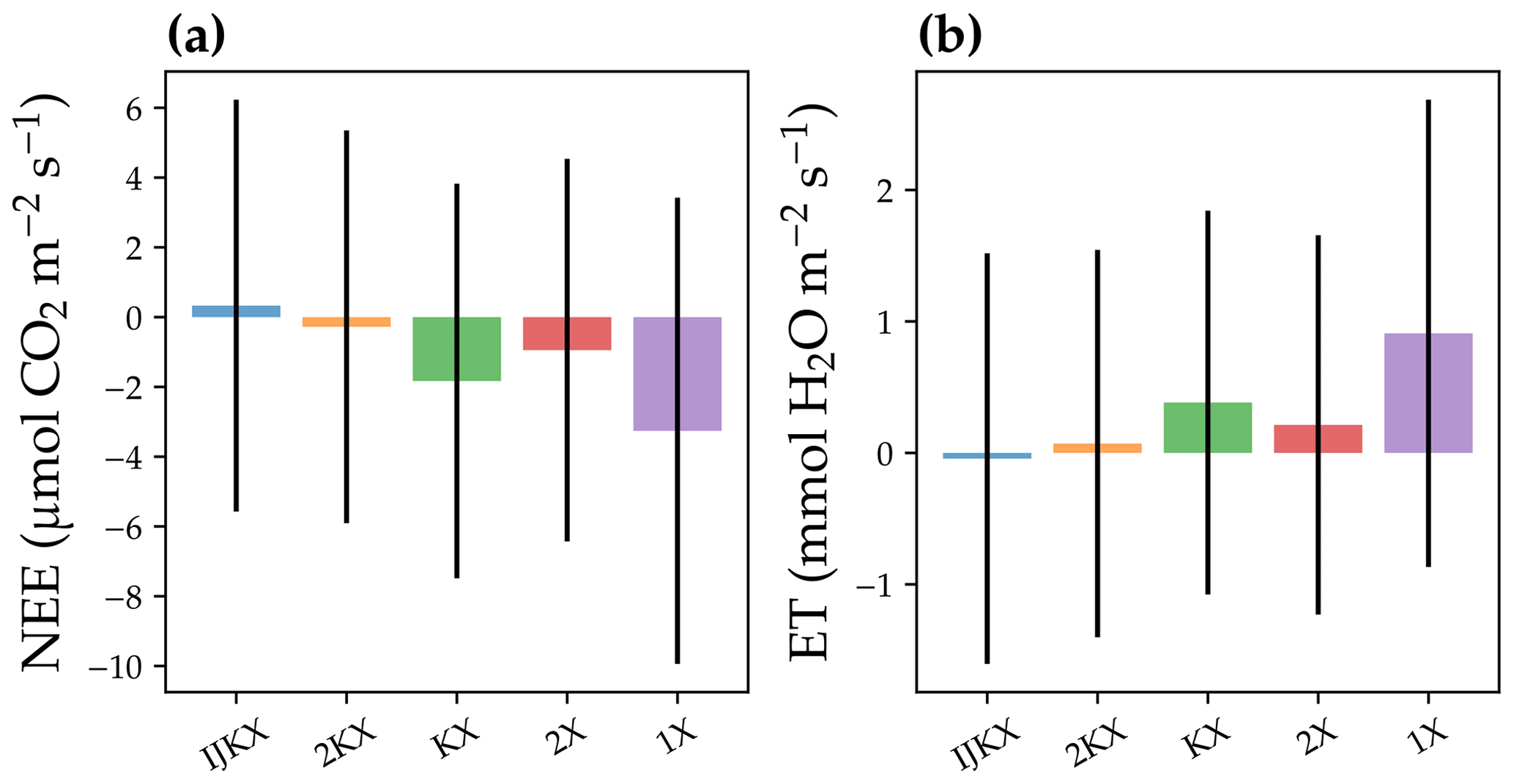
Figure 8 Difference between five different canopy complexity levels in a diurnal-cycle simulation of carbon and water fluxes. The carbon flux was represented by the site-level net ecosystem exchange of CO₂ (NEE). The water flux was represented by site-level evaporation transpiration using plant transpiration as a proxy (ET). The bars plot the mean difference between model simulation and observations, and error bars plot 1 standard deviation. The observation was from a flux tower at Ozark, Missouri, USA (US-MOz). The model simulations were run with a profile of vertical leaf photosynthetic capacity using observed weather drivers from day 177 to 179 in the year 2019, such as air and soil humidity. For NEE, negative values stand for overestimated carbon fluxes; for ET, positive values stand for overestimated water fluxes.

3.2 Diurnal cycle

Our model simulations suggest that all tested canopy complexity levels can qualitatively capture the trends of carbon and water fluxes at the tested flux tower site (Fig. 7). However, the tested complexity levels differed dramatically in the magnitudes of carbon and water fluxes. In general, 1X had the highest fluxes for both carbon and water fluxes (represented by NEE and ET), followed by KX, 2X, 2KX, and IJKX (Figs. 7 and 8). Though 2KX and 2X, in general, had relatively small differences from IJKX, we were still able to distinguish the difference (Figs. 7 and 8). We note here again that Figs. 7 and 8 were meant to highlight the difference between canopy complexity levels in model simulations but not to say that some models were better than others.

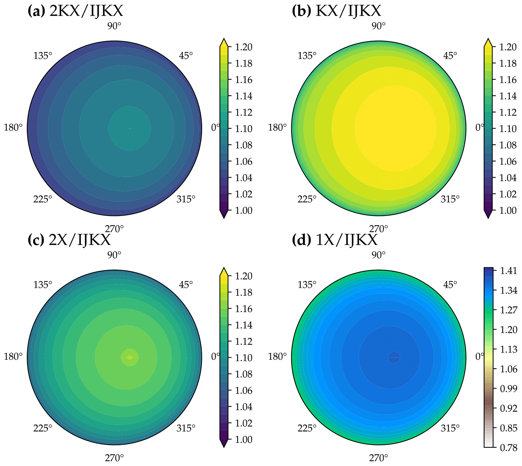
Figure 9 Difference between five different canopy complexity levels in modeled solar-induced chlorophyll fluorescence (SIF) at a different viewing zenith angle and relative azimuth angle. The color indicates SIF at 740 nm of a tested canopy complexity level relative to IJKX. The model simulations were run with a profile of vertical leaf photosynthetic capacity using observed weather drivers at 12:00–12:30 of day 177 in the year 2019 at a flux tower at Ozark, Missouri, USA (US-MOz).

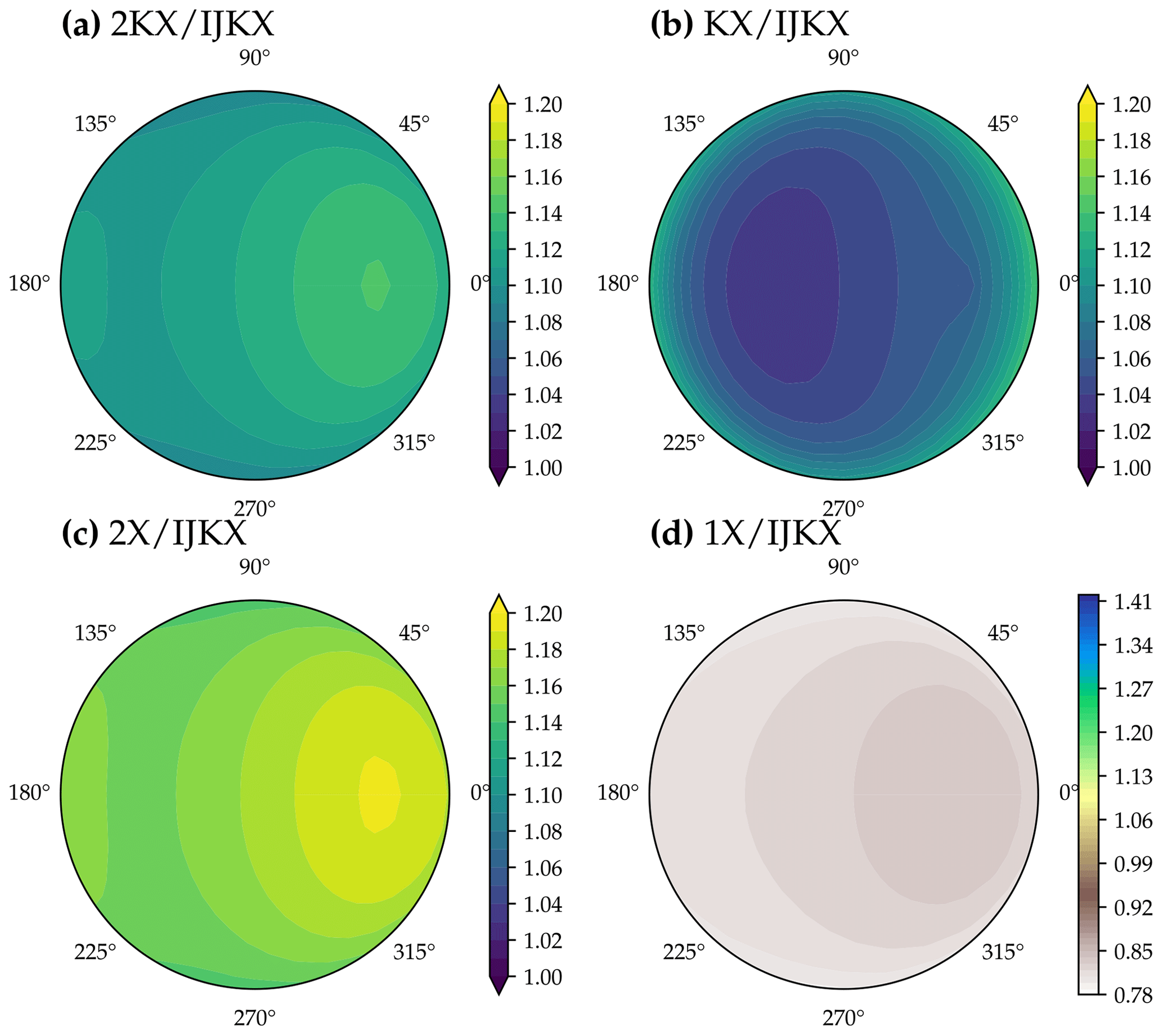
Figure 10 Difference between five different canopy complexity levels in modeled solar-induced chlorophyll fluorescence (SIF) at different viewing zenith angle and relative azimuth angle. The color indicates SIF at 740 nm of a tested canopy complexity level relative to IJKX. The model simulations were run with a profile of vertical leaf photosynthetic capacity using observed weather drivers at 16:00–16:30 of day 177 in the year 2019 at a flux tower at Ozark, Missouri, USA (US-MOz).

3.3 Sun-sensor geometry

Using less complicated canopy complexity (namely 2KX, KX, 2X, and 1X) impacted the observed SIF depending on the sun-sensor geometry (Figs. 9 and 10). For the tested time window at 12:00–12:30, 2KX has the least difference from IJKX, followed by 2X, KX, and 1X. In general, 2KX had a difference lower than 11 % at any viewing zenith angle or relative azimuth angle for the tested time window (Figs. 9). The impact of sun-sensor geometry changed with time because of changes in solar zenith angle and total radiation (e.g., at 16:00–16:30 in the afternoon; Fig. 10). While 2KX still had lower overestimated SIF compared to 2X, KX had better agreement with IJKX, and 1X even underestimated SIF. The dramatic changes in SIF from KX and 1X were due to lower incident radiation from 16:00 to 16:30 (Fig. 5a).

Figure 11 Leaf fluorescence responses to radiation, CO₂ partial pressure, and the leaf maximum carboxylation rate. (a) Photosynthesis system II quantum yield responses to leaf absorbed photosynthetically active radiation (APAR) and leaf internal CO₂ partial pressure. (b) Leaf fluorescence quantum yield (ϕ_F) responses to APAR and leaf internal CO₂. (c) Product of ϕ_F and APAR vs. APAR for leaves with different internal CO₂ (number labeled next to each curve; unit: Pa). (d) Product of ϕ_F and APAR vs. internal CO₂ at different APAR values (number labeled next to each curve; unit $\mathrm{\mu }\mathrm{mol}{\mathrm{m}}^{-\mathrm{2}}{\mathrm{s}}^{-\mathrm{1}}$). The simulations of panels (a–d) are done at a leaf temperature of 25 ^∘C and a maximum carboxylation rate (V_cmax) of 60 $\mathrm{\mu }\mathrm{mol}{\mathrm{CO}}_{\mathrm{2}}{\mathrm{m}}^{-\mathrm{2}}{\mathrm{s}}^{-\mathrm{1}}$. (e) ϕ_F of different canopy layers was at a given atmospheric CO₂ partial pressure. V_cmax was the same among canopy layers. The simulation results are from Fig. 4e. (f) ϕ_F of different canopy layers was at a given atmospheric CO₂. V_cmax was lower in the lower canopy. The simulation results are from Fig. 5e.

4 Discussion

4.1 Fluorescence and radiation

While simpler canopy models in general predicted higher carbon, water, and SIF fluxes, there were some scenarios that the simpler models predict contrasting SIF responses compared to IJKX: (a) when total radiation increased, SIF of the simpler canopy models was lower than that of IJKX at low radiation but were higher than that of IJKX at high radiation (Figs. 4 and 5); (b) 1X model SIF increased and then decreased and stayed unchanged with higher atmospheric CO₂ (Figs. 4 and 5); and (c) KX model SIF increased marginally with higher atmospheric CO₂ for a canopy without a vertical V_cmax gradient but decreased with higher CO₂ for a canopy with a vertical V_cmax profile (Figs. 4 and 5). These contrasting patterns of the simpler models resulted from the different photosynthesis system II (PSII) quantum yield and fluorescence quantum yield (namely ϕ_F) responses to APAR and CO₂ (Fig. 11a, b). The PSII quantum yield measures the efficiency of converting absorbed photons to electrons by PSII; and ϕ_F measures the efficiency of converting absorbed photons to fluorescence photons. The PSII yield increases and then saturates with higher leaf internal CO₂ and lower APAR. In our model, ϕ_F follows the parameterization of van der Tol et al. (2014) but fitted on leaves measured by Flexas et al. (2002), as first used in Lee et al. (2015). Typically, the PSII-to-ϕ_F relationship depends on the state of non-photochemical quenching (NPQ; Porcar-Castell et al., 2014). ϕ_F has a maximum at intermediate PSII levels (around 0.6) but decreases at lower PSII yields (increased NPQ) as well as higher PSII yields (increased competition with photochemical quenching). This general behavior explains what we see the following: ϕ_F (a) stays unchanged at low radiation with higher leaf internal CO₂, (b) increases and then decreases and stays unchanged with higher leaf internal CO₂ at intermediate APAR, (c) increases with higher CO₂ at high CO₂, and (d) increases and then decreases with higher APAR (Fig. 11a, b). Though ϕ_F in general agrees with the PSII yield patterns at high APAR (typical experimental and top-of-canopy scenarios), the disagreements at low APAR could result in problems when APAR is inappropriately averaged. In our case, the turnover from APAR regions in which PSII and ϕ_F are anticorrelated (light-limited) to the region in which they are correlated (increase in NPQ) happens at around 200 µmol m² s⁻¹.

When total radiation was higher, the product of ϕ_F and APAR (leaf-level SIF) increased (Fig. 11c). When ϕ_F stayed unchanged at low APAR, leaf-level SIF increases linearly with higher APAR, and SIF increases faster when ϕ_F starts to increase after a certain threshold (the threshold increased with higher leaf internal CO₂; Fig. 11b). Then leaf-level SIF slowed down with higher APAR due to decreasing ϕ_F at higher APAR and was higher when leaf internal CO₂ was higher (Fig. 11b, c). As leaf internal CO₂ was theoretically lowest for 1X, then followed by KX, 2X, and 2KX given the way APAR was averaged, it was expected that 2KX increased earliest with higher APAR and that 1X had the highest SIF value at high radiation (Figs. 4a and 5a). Therefore, in the diurnal-cycle simulations, 1X SIF overestimated SIF at noon when radiation was high (Fig. 9) but underestimated SIF in the late afternoon as a result of lower radiation (Fig. 10). The inconsistent SIF patterns at low and high radiation from simpler canopy models may potentially result in biases in modeled diurnal and seasonal SIF, and thus we suggest using a complex canopy model when possible to minimize the impact from heterogeneous canopy radiation and leaf physiology.

The 1X model SIF response to atmospheric CO₂ ought to depend on the mean canopy APAR (Fig. 11b): (a) if mean APAR was low, 1X SIF should stay constant with higher CO₂; (b) if mean APAR was moderate, 1X SIF ought to increase and then decrease and stay constant with higher CO₂; and (c) if mean APAR was high, 1X SIF would increase with higher CO₂ (Fig. 11b, d). For the simulations in Figs. 4 and 5, mean APAR was 156 $\mathrm{\mu }\mathrm{mol}{\mathrm{m}}^{-\mathrm{2}}{\mathrm{s}}^{-\mathrm{1}}$, and thus 1X SIF increased and then decreased with higher CO₂.

The KX model SIF response to atmospheric CO₂ was impacted by both leaf internal CO₂ and the vertical APAR profile given the heterogeneous APAR. As ϕ_F was higher in the middle layers at lower atmospheric CO₂ when there is no vertical V_cmax gradient, modeled SIF showed marginal increase with higher CO₂ (Figs. 4 and 11e). However, when there was a vertical V_cmax gradient, ϕ_F was much higher in the lower canopy at lower CO₂, potentially resulting in higher SIF at low atmospheric CO₂, which was contrary to the IJKX prediction. The erroneous predicted SIF patterns of 1X and KX highlighted the importance of appropriately averaged leaf APAR, particularly the partitioning of sunlit and shaded leaves.

4.2 Dataset compatibility

Our model simulations showed that different canopy complexity levels predicted divergent carbon, water, and SIF fluxes. 1X and KX without partitioning the canopy to sunlit and shaded fractions, in particular, showed very high biases compared to the other three levels of complexity, namely 2X, 2KX, and IJKX. Further, as we expected, IJKX, which has the most complex canopy, had the lowest predicted carbon and water fluxes, followed by 2KX and 2X and then KX and 1X. Moreover, when we accounted for a profile of vertical canopy photosynthetic capacity, the difference among canopy complexity levels increased. Though 2KX and 2X were, in general, close to IJKX in predicted canopy fluxes, the disagreements may range up to > 20 % (maximum) for 2KX and up to > 40 % (maximum) for 2X. Given the differences in predicted fluxes using different canopy complexity levels and the varying difference (not a constant ratio), we do not recommend using photosynthetic parameters inverted from different canopy complexity models; i.e., parameter fitting has to be performed with the same underlying model as for the full forward modeling. Given the higher realism of the enhanced complexity models, however, leaf-level fits of photosynthetic parameters could be employed in models of higher complexity but would result in high biases when used in simple big-leaf models.

The disagreements among canopy complexity levels make it difficult to parameterize a land model using a complex canopy setup and thus hamper the fusion of large-scale remote-sensing-based datasets with land models at a global scale. Thus, it is necessary to revisit the flux and plant trait inversions using more applicable land model setups to make sure the inverted datasets and land models are consistent in their assumptions. This is the only way to ensure that inverted parameters are quantitatively useful in future land surface modeling. Moreover, it is also possible for land models to go without the inverted fluxes or traits if the land model runs using a complex canopy such as IJKX. This way, the model can be directly compared against satellite observations (Shiklomanov et al., 2021) without an intermediate step that performs the inversion from radiation observation canopy properties and thus surface water and carbon fluxes.

4.3 Necessity of a complex canopy

As suggested by Bonan et al. (2021), modelers need to move to a multi-layered canopy modeling to account for the vertical profiles and microclimates in the canopy. Further, to better utilize the broadly available remote sensing data, modelers need to move from broadband radiation to hyperspectral radiation and from sun/shade fractions to leaf angular distribution. One may ask whether it is necessary to implement a way more complex and inefficient multi-layered canopy with leaf angular distributions to account for an average 5 %–22 % difference, while the difference can be compensated by tuning plant traits such as photosynthetic capacity and hydraulic conductance. The answer varies depending on what types of data are used in the model. If one uses parameters meant to use with 2X (namely a two-leaf canopy), using a multi-layered canopy such as 2KX and IJKX would not improve the model performance but instead could result in higher biases. In this case, we suggest keeping the same canopy complexity as used to derive plant traits. However, if one wants to bridge plant physiology to both leaf-level measurements as well as remotely sensed data such as the reflection and fluorescence spectra, we would suggest using IJKX or using an even more complicated canopy model to be as accurate as possible. We note here that 2KX approximates IJKX well with an average 3 %–12 % difference, and 2KX would be useful to speed the calculations for more qualitatively oriented research as the trends generally agree between 2KX and IJKX.

We recognize that increasing model complexity can make it (a) less user-friendly for researchers to use (e.g., when implementing the model into their research projects) and (b) slower to run the model, particularly using less efficient programming languages such as Python and R (compared to C). In our highly modularized CliMA Land model, we use Julia, a just-in-time compiled programming language that allows for the versatility of a scripting language like Python but with the speed of fully compiled languages such as C and Fortran (see https://julialang.org/benchmarks/, last accedss: 22 December 2021). The CliMA Land model can simulate canopy radiation using either the mSCOPE-based radiative transfer scheme (Yang et al., 2017) or the traditional sunlit- and shaded-fraction scheme (e.g., De Pury and Farquhar, 1997; Campbell and Norman, 1998). Further, CliMA Land supports both stomatal optimization models (including those from Sperry et al., 2017; Anderegg et al., 2018; Eller et al., 2018; Wang et al., 2020) and empirical stomatal models (including those from Ball et al., 1987; Leuning, 1995; Medlyn et al., 2011). For the empirical stomatal models, CliMA Land supports using an ad hoc tuning factor to account for stomatal responses to soil moisture through tuning either the empirical fitting parameter (such as g₁ in the Ball et al., 1987, and Medlyn et al., 2011, models) or the leaf photosynthetic capacity (as done in Kennedy et al., 2019). Users may freely customize the model setup by choosing among the provided alternatives. We believe the practice of making land models more open and modular will benefit the land model and plant physiology communities in future research.

5 Conclusions

We evaluated how much canopy carbon, water, and SIF fluxes differ when using five different canopy complexity levels in a land model. We found that when using the same model inputs, simpler canopy models predicted higher carbon, water, and SIF fluxes, and when we accounted for a profile of vertically heterogeneous photosynthetic capacity, we found more disagreements among canopy models with varying complexity levels. We also found that the modeled SIF varied with sun-sensor geometry among tested canopy complexity levels. Our model results suggest that misusing parameters inverted from different canopy complexities and assumptions may have resulted in biases in predicted canopy fluxes, and thus we recommend more cautious model parameterization regarding canopy complexity levels. Further, we recommend using complex canopy models with leaf angular distribution and a hyperspectral radiation transfer scheme to compare against remote sensing data in order to accurately mimic observed radiation. However, the use of complex canopy models in land surface modeling may be less efficient and not user-friendly for researchers. We believe more open and modular land models like CliMA Land will help lower the threshold to researchers.