Wintertime process study of the North Brazil Current rings reveals the region as a larger sink for CO₂ than expected

The key processes driving the air–sea CO₂ fluxes in the western tropical Atlantic (WTA) in winter are poorly known. WTA is a highly dynamic oceanic region, expected to have a dominant role in the variability in CO₂ air–sea fluxes. In early 2020 (February), this region was the site of a large in situ survey and studied in wider context through satellite measurements. The North Brazil Current (NBC) flows northward along the coast of South America, retroflects close to 8^∘ N and pinches off the world's largest eddies, the NBC rings. The rings are formed to the north of the Amazon River mouth when freshwater discharge is still significant in winter (a time period of relatively low run-off). We show that in February 2020, the region (5–16^∘ N, 50–59^∘ W) is a CO₂ sink from the atmosphere to the ocean (−1.7 Tg C per month), a factor of 10 greater than previously estimated. The spatial distribution of CO₂ fugacity is strongly influenced by eddies south of 12^∘ N. During the campaign, a nutrient-rich freshwater plume from the Amazon River is entrained by a ring from the shelf up to 12^∘ N leading to high phytoplankton concentration and significant carbon drawdown (∼20 % of the total sink). In trapping equatorial waters, NBC rings are a small source of CO₂. The less variable North Atlantic subtropical water extends from 12^∘ N northward and represents ∼60 % of the total sink due to the lower temperature associated with winter cooling and strong winds. Our results, in identifying the key processes influencing the air–sea CO₂ flux in the WTA, highlight the role of eddy interactions with the Amazon River plume. It sheds light on how a lack of data impeded a correct assessment of the flux in the past, as well as on the necessity of taking into account features at meso- and small scales.

1 Introduction

The North Brazil Current (NBC) is one of the dominant features of the tropical Atlantic circulation. In a region dominated by zonal jets, it flows northward along the coast of South America and separates from the coast around 6–8^∘ N. The NBC seasonally turns back on itself in a tight loop, called the NBC retroflection, and feeds the North Equatorial Counter Current, closing off the equatorial wind-driven gyre (Fig. 1). This retroflection occasionally pinches off some of the world's largest eddies, the North Brazil Current rings (Johns et al., 1990; Richardson et al., 1994).

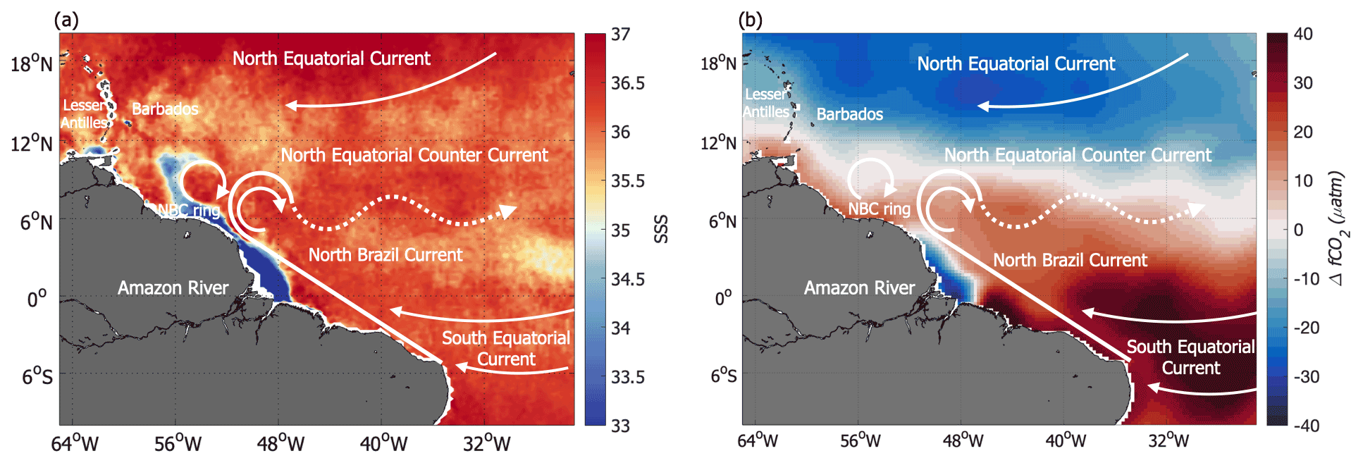
Figure 1 Schematic of the main ocean currents in the western tropical Atlantic superimposed over the SSS field of 7 February 2017 (a) and over the February ΔfCO₂ climatology from Landschützer et al. (2020) (b).

After their separation from the NBC retroflection region, the rings travel northwestward toward the Lesser Antilles in a course parallel to the coast of South America. These eddies have been extensively studied using modelling and both in situ (e.g. 1998–2001 NBC Ring experiment; Wilson et al., 2002) and satellite observations (e.g. Goni and Johns, 2001; Fratantoni and Glickson, 2002; Aroucha et al., 2020). They have a mean radius of 200 km, and their diameter can exceed 450 km. Vertically, some of them extend down to more than 1000 m (Fratantoni and Glickson, 2002; Fratantoni and Richardson, 2006; Johns et al., 2003). The NBC rings swirl clockwise and travel with an average northwestward translation speed of 8–15 km d⁻¹ (Johns et al., 1990; Mélice and Arnault, 2017). Most of the anticyclonic eddies detectable by altimetry are rather shallow, extending from the surface to 200–300 m (Garraffo et al., 2003; Wilson et al., 2002). When they reach the Lesser Antilles, they start to coalesce and disintegrate partly due to interactions with the topography (Fratantoni and Richardson, 2006; Jochumsen et al., 2010). There is substantial variability in the number of rings shed per year, ranging from five (Aroucha et al., 2020; Fratantoni and Glickson, 2002; Mélice and Arnault, 2017; Goni and Johns, 2001) to nine (Johns et al., 2003). NBC rings play a crucial role in the inter-hemispheric transport of salt and heat in the Atlantic Ocean and are an important part of the meridional overturning circulation (Johns et al., 2003). The NBC rings disrupt an already complex region located in the vicinity of the Amazon River mouth and at the transition between equatorial and subtropical waters. While most of the studies on rings focused on their physical properties, little is known about their biogeochemical properties and how they affect the air–sea CO₂ flux of the western tropical Atlantic.

The global ocean acts as an atmospheric CO₂ sink, taking up 23 % of total anthropogenic CO₂ emissions (Friedlingstein et al., 2020) and leading to ocean acidification (Masson-Delmotte et al., 2021; Pörtner et al., 2019). The concentration of atmospheric CO₂ is increasing due to human activities (IPCC, 2019, 2021), and characterizing the role of the ocean in mitigating climate change through CO₂ uptake is thus a key investigation. The equatorial Atlantic Ocean is the second-largest source of CO₂ to the atmosphere after the equatorial Pacific (Landschützer et al., 2014; Takahashi et al., 2009). Previous works in this region examined the influence of the equatorial upwelling and of the Amazon plume on the CO₂ flux. CO₂-rich equatorial waters, originating from the equatorial upwelling (Andrié et al., 1986), strongly contrast with the CO₂-undersaturated Amazon River plume waters. The magnitude of the Amazon River discharge is unique in the global ocean. It represents as much freshwater as the next seven largest rivers in the world combined and contributes to almost 20 % of global river freshwater input to the ocean (Dai and Trenberth, 2002). It therefore strongly impacts the physical, biogeochemical and biological properties of the coastal and the open ocean. Often overlooked, the Amazon River plume is an atmospheric CO₂ sink of global importance (Ibánhez et al., 2016). The plume carries water rich in silicate, nitrogen and phosphate into the tropical oceanic waters that are strongly depleted in nutrients. As water mixes and turbidity decreases, the primary producer's growth and associated biological drawdown are stimulated (Chen et al., 2012). Nitrogen is rapidly consumed, and nitrogen fixation by diazotrophs becomes the main pathway of carbon sequestration in the plume (Subramaniam et al., 2008). This strong carbon drawdown leads to a significant sink of atmospheric CO₂ (Körtzinger, 2003; Lefèvre et al., 2010). Not taking into account the Amazon plume would result in overestimating the tropical Atlantic air–sea CO₂ flux by 10 % (Ibánhez et al., 2016).

The Amazon River's discharge reaches a minimum in December and progressively increases from January onwards. The plume extension is minimum from January to March (Fournier et al., 2015), and as a result, it is the period of maximum salinity in the northwestern tropical Atlantic. The Amazon outflow region is particularly hard to reconstruct due to its strong variability and a severe lack of data. Waters located in the southeasternmost part of the domain act as a strong source of CO₂ to the atmosphere. The source gradually turns into a sink north of 10^∘ N as waters become colder due to seasonal winter cooling. This situation is typical of a transition zone between equatorial and subtropical waters in winter (Landschützer et al., 2020; Fig. 1b). The northwestern tropical Atlantic is commonly divided into two parts: the northern much less variable part (also called “Trade wind region”) and the southern part, also referred to as Eddy Boulevard (Stevens et al., 2021). The freshwater of the Amazon remains mainly confined to the continental shelf due to winds perpendicular to the coast as it travels northwestward into the Caribbean Sea (Coles et al., 2013). However, it has recently been documented that off-shore freshwater transport is often present in February and significantly alters the physical properties of the region (Reverdin et al., 2021). This is partly due to the interaction of the NBC rings with the Amazon plume (Fig. 1a). The ocean colour signature of the Amazon (Muller-Karger et al., 1988) has been used as a tracer to delineate the rings and better understand their generation, evolution and characteristics (Johns et al., 1990; Fratantoni and Glickson, 2002). The Amazon River also influences the surface temperature and salinity of the rings. For example, Fig. 1a shows a freshwater plume stirred by a large ring. They are considered warm-core rings but have a warm sea surface temperature (SST) anomaly in the first half of the year and a cold one in the second half because the anomaly is relative to the regional SST, with an extensive warm pool in late summer and autumn (Ffield, 2005). Their signature in salinity is therefore plume-dependent as well. Ffield (2005) reported that three out of four rings were surrounded by lower-salinity water. Salinity and chlorophyll a are therefore critical to understand the surface physical and biogeochemical properties of the region, as well as the air–sea fluxes of CO₂.

The northwestern tropical Atlantic is a dynamically active region, with eddies several hundred kilometres in diameter and connected to the world's largest river. There are surprisingly few biogeochemical observations available for winter months during low outflow of the Amazon River. Few tropical Atlantic measurements of biogeochemical tracers are available, with one transect in winter in the Surface Ocean CO₂ Atlas (SOCAT; Bakker et al., 2016) database south of 10^∘ N crossing the region. This scarcity is a major impediment in understanding the biological and physical processes underlying the oceanic carbon and nutrient cycles in the region. Satellite salinity shows a contrasted spatial structure with eddies and filaments (Fig. 1a). In this study, we take advantage of the physical and biogeochemical data collected during the EUREC⁴A-OA/ATOMIC (Elucidating the Role of Clouds–Circulation Coupling in Climate Ocean–Atmosphere and Atlantic Tradewind Ocean–Atmosphere Mesoscale Interaction Campaign) experiment in January–February 2020, combined with satellite data, to understand how the NBC rings and their related structures impact the air–sea CO₂ flux in winter. The paper is organized as follows. We present the in situ observational data from the EUREC⁴A-OA/ATOMIC experiment, as well as the satellite data, in Sect. 2. We identify the water masses observed in the region and their physical and biogeochemical properties and estimate the CO₂ fluxes at regional scale using empirical relationships in Sect. 3. In Sect. 4, we compare the results with climatologies of air–sea CO₂ fluxes to evaluate the added knowledge brought by the intensive surveys of February 2020. We discuss the results and the inter-annual variability in Sect. 4, and we conclude in Sect. 5.

2 Data and methods

2.1 In situ data

The EUREC⁴A-OA/ATOMIC (Stevens et al., 2021) campaign took place in January and February 2020 and involved research vessels (RVs) from France (RV Atalante; Speich and The Embarked Science Team, 2021), Germany (RV Maria S. Merian, hereby designated as Merian; Karstensen et al., 2020; and RV Meteor, not considered in this study since no CO₂ measurements were taken on board) and the United States (RV Ronald H. Brown, hereby designated as Ron Brown; Quinn et al., 2021). These cruises provided numerous in situ measurements, and, in this study, we will focus on the continuous near-surface measurements of temperature, salinity and fCO₂.

Temperature and salinity from thermosalinographs (TSGs), as well as fCO₂, were measured from water pumped ∼5 m below the surface. For each ship, the resulting CO₂ data are corrected (Lefèvre et al., 2010; Pierrot et al., 2009) from the temperature difference between the water at the ship's water intake and the one analysed by the instrument. RV Atalante fCO₂ measurements started on 30 January and ended on 18 February 2020 (Olivier et al., 2020). The underway oceanic and atmospheric fCO₂ were detected by infrared detection using a LI-COR LI-7000 (Takahashi et al., 1993). The fCO₂ system was the same as in Lefèvre et al. (2010). It uses a shower air–sea equilibrator described by Poisson et al. (1993). Seawater from the TSG pumping circuit circulates in the equilibrator at a rate of 2 L min⁻¹. A closed loop of about 100 mL of air flows through the equilibrator designed to avoid bubbles at the air–sea interface. To minimize temperature corrections, the equilibrator is thermostated with the same seawater as the one used for CO₂ measurements. The temperature difference between the equilibrator and the sea was on the order of 0.5 ^∘C.

Furthermore, 138 samples for dissolved inorganic carbon (DIC) and total alkalinity (TA) analysis were collected on board RV Atalante, as well as inorganic nutrients (silicate, phosphate, nitrate and nitrite). DIC and TA were measured at the SNAPO-CO₂ (French National Facility for Analysis of Carbonate System Parameter) facility by potentiometric titration using a closed cell, following the method of Edmond (1970). Nutrients were conserved by heat pasteurization and analysed by colourimetry at IRD LAMA service in Brest.

An OceanPack CUBE FerryBox system from SubCtech was installed on RV Merian measuring continuously the oceanic fCO₂ from 23 January to 19 February 2020. Water is pumped at a rate of ∼7 L min⁻¹ through a debubbler unit subsequently followed by a SeaBird SBE 45 thermosalinograph before it circulates along a membrane through which CO₂ diffuses. On the other side of the membrane, the air loop is circulated at a rate of 0.5 L min⁻¹ through a LI-COR LI-840 non-dispersive infrared gas analyser (e.g. Arruda et al., 2020). RV Ron Brown completed two legs, from 10 to 25 January and from 29 January to 13 February 2020. The General Oceanic Inc. 8500 pCO₂ instrument installed on board follows a similar methodology to the underway fCO₂ system deployed on the Atalante and is detailed in Pierrot et al. (2009).

An inter-comparison of the fCO₂ measured by RVs Atalante and Merian is attempted when the ships were navigating together at a distance of less than 5 km (Fig. 2). On average, the fCO₂ measured by RV Merian is 6.4 µatm higher than the one measured on RV Atalante, with a standard deviation of 4.8 µatm. RVs Merian and Ron Brown crossed the same water mass at 13–14^∘ N, 57^∘ W on 12 February. On average, RV Merian fCO₂ is 6 µatm higher than RV Ron Brown fCO₂. In part we link these differences to the slower response time of the membrane system; however, differences also lie within the uncertainties of the fCO₂ observing systems (∼5 µatm for the membrane system installed on RV Merian, see Arruda et al., 2020, and ∼2 µatm for the equilibrator systems installed on RVs Atalante and Ron Brown). The region where RV Merian and RV Atalante were close is very variable (standard deviation of 20 µatm), and RV Merian and RV Ron Brown were never in the same place at the same time, so the observed differences could also be due to the natural variability in fCO₂ sampled differently by the various ships. Hence, we did not apply any correction, and we checked that the effect of a 6 µatm systematic bias in RV Merian fCO₂ had a minor effect on our resulting interpolations. A comparison between the reconstructed flux with and without a correction for the 6 µatm systematic bias suggests that such a systematic bias would lead to less than 2 µatm difference in our mean interpolated fCO₂ and less than 0.1 $\mathrm{mmol}{\mathrm{m}}^{-\mathrm{2}}{\mathrm{d}}^{-\mathrm{1}}$ in the mean derived air–sea CO₂ flux.

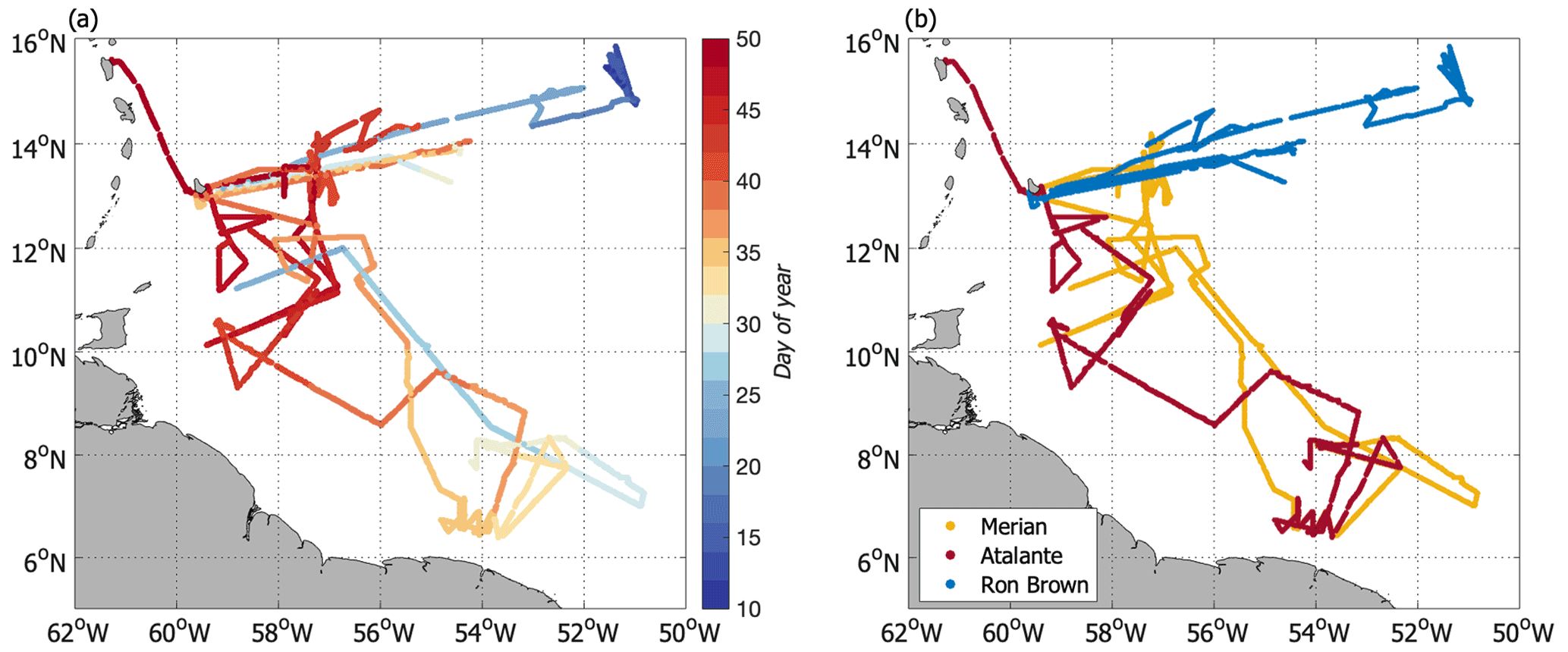
Figure 2 Ship tracks colour-coded by day of year (a) and by ship name (b).

2.2 Satellite and atmospheric reanalysis data

Daily satellite maps of chlorophyll-a (chl a) and SST, as well as absolute dynamic topography (ADT) and sea surface salinity (SSS), are used in this study.

The salinity maps are a blend of the Soil Moisture Ocean Salinity (SMOS, January 2010–present) and Soil Moisture Active Passive (SMAP, April 2015–present) measurements developed by Reverdin et al. (2021). The European SMOS and US SMAP missions observe the sea surface by L-band radiometry from sun-synchronous polar-orbiting satellites (Entekhabi et al., 2010; Font et al., 2009; Kerr et al., 2010; Piepmeier et al., 2017). Combining 06:00 and 18:00 local time measurements of both missions provides an almost complete coverage each day. When the coverage was not complete over our region, the 06:00 track of the following day was also included. This daily field is available for the first 20 d of February and leaves out only 2 d without sufficient coverage to retrieve salinity data. It has a spatial resolution close to 70 km and an uncertainty on the order of 0.5. This product is optimized for the northwestern tropical Atlantic in February 2020 and has an almost daily resolution. It is an experimental daily product built to have the best representation possible of the Amazon plume variability. The product, its uncertainties and the comparison between the TSG salinity and the satellite SSS are detailed in Reverdin et al. (2021).

Daily chl a concentration maps and SST maps are produced by CLS (Stum et al., 2016) on a spatial grid of 0.02^∘. The chl a concentration maps are composites built from VIIRS (Visible Infrared Imaging Radiometer Suite; on Suomi NPP (Suomi National Polar-orbiting Partnership) and NOAA-20 US platforms) and OLCI (Ocean and Land Colour Instrument; on Sentinel 3A and 3B Copernicus European platforms) satellite sensors. The SST product is a 1 d average of infrared radiometer satellite data. Both datasets are sensitive to the cloud cover, but during our period of interest, they are usually without many gaps except at the end of February. The comparison between the TSG SST and the satellite SST product is detailed in RV Atalante's cruise report (Speich and The Embarked Science Team, 2021).

Daily ADT maps at a $\mathrm{1}/\mathrm{4}$^∘ resolution combine data from all satellites available for the period 1993 to present. From these ADT fields, the TOEddies algorithm, developed by Laxenaire et al. (2018), identifies eddies and their trajectories. The eddy detection is based on the closed contours of ADT, as well as the maximum geostrophic velocity associated with the eddy.

In order to compute the air–sea CO₂ fluxes, the European Centre for Medium-Range Weather Forecasts (ECMWF) Reanalysis v5 (ERA5) hourly wind speed and mean sea level pressure, P_atm, are used. ERA5 covers the period from January 1950 to present and provides hourly data on a 30 km grid. In addition, the monthly wind speed and SST fields over the period 1998–2015 are used, and a climatology over this period is computed. The wind speed in the region in winter is on average between 6 and 8 m s⁻¹, and its variability is low.

We compare the EUREC⁴A-OA/ATOMIC observations with the observation-based CO₂ partial pressure (pCO₂) climatology developed by Landschützer et al. (2020), created using a two-step neural network method (Landschützer et al., 2016) and combining open and coastal ocean datasets. The associated ΔpCO₂ and air–sea CO₂ flux monthly field climatologies over the 1998–2015 period are computed using the ERA5 climatological wind, SST and P_atm fields, as well as the atmospheric CO₂ from the Ragged Point, Barbados, station.

2.3 Methods

2.3.1 Air–sea CO₂ flux

We compute the air–sea flux (F; $\mathrm{mmol}{\mathrm{m}}^{-\mathrm{2}}{\mathrm{d}}^{-\mathrm{1}}$) as follows:

$$\begin{array}{}\text{(1)}& F=k\cdot K_{\mathrm{0}}\cdot (f{\mathrm{CO}}_{\mathrm{2}}-f{\mathrm{CO}}_{\text{2atm}}),\end{array}$$

where K₀ is the solubility of CO₂ in seawater, expressed as a function of SSS and SST by Weiss (1974); fCO_2atm is the atmospheric CO₂ fugacity; and k is the gas transfer velocity. k is calculated following the relation from Wanninkhof (2014):

$$\begin{array}{}\text{(2)}& k=\mathrm{0.251}\cdot \langle U^{\mathrm{2}}\rangle \cdot (\mathit{Sc}/\mathrm{660}{)}^{-\mathrm{0.5}},\end{array}$$

where Sc is the Schmidt number, and U is the wind speed at 10 m above sea level derived from ERA5 wind speed. The ERA5 wind speed is used for the satellite-based analysis and the air–sea CO₂ flux climatology. The measured winds from the ships are adjusted to 10 m following a logarithmic profile (Tennekes, 1973) and used to compute the along-track flux for visualization purposes.

In order to compute fCO_2atm over that period, we first derived the saturation vapour pressure ($P_{{\mathrm{H}}_{\mathrm{2}}\mathrm{O}}$) from SSS and SST and then the atmospheric pCO₂ using the monthly averaged CO₂ mole fraction (xCO_2atm) measured at the NOAA/Earth System Research Laboratory (ESRL) station in Ragged Point, Barbados (13.17^∘ N, 59.43^∘ W):

$$\begin{array}{}\text{(3)}& f{\mathrm{CO}}_{\text{2atm}}=x{\mathrm{CO}}_{\text{2atm}}\cdot (P_{\text{atm}}-P_{{\mathrm{H}}_{\mathrm{2}}\mathrm{O}})\cdot C_{\mathrm{f}},\end{array}$$

where C_f is the fugacity coefficient, a function of the atmospheric pressure and SST (Weiss, 1974).

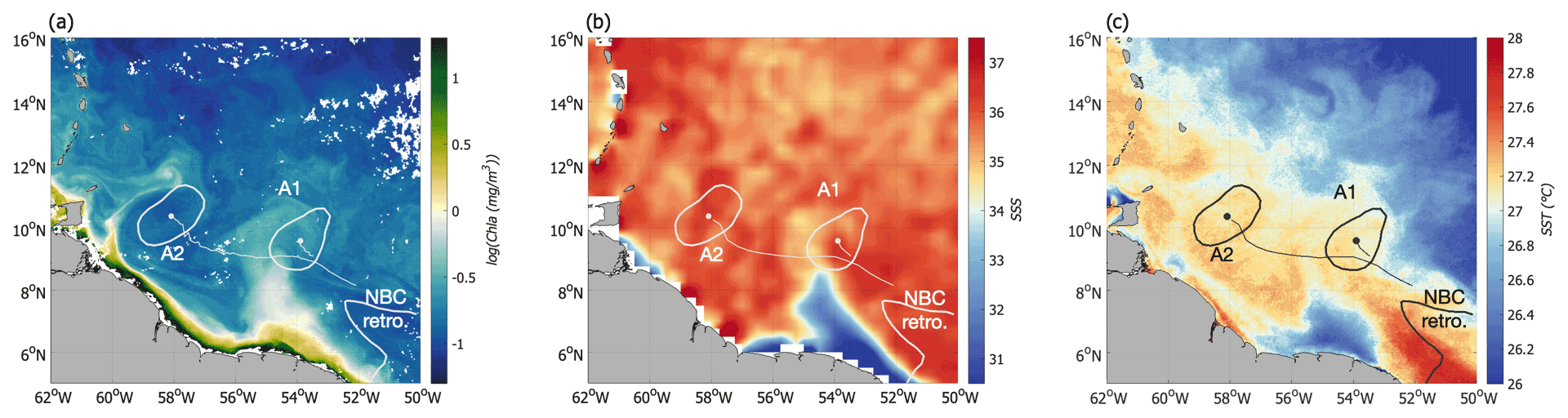
Figure 3 (a) Chlorophyll a, (b) SSS and (c) SST on 6 February 2020 with the contours of NBC rings A1 and A2, their centre, and their trajectory. The NBC retroflection is identified from the 0.51 m contour of the satellite-derived ADT.

2.3.2 Reconstruction of fCO₂ from satellite maps

Our approach is to derive from the large EUREC⁴A-OA dataset a relationship linking fCO₂ to SST, SSS and chl a in order to provide maps of fCO₂ based on the satellite maps of SST, SSS and chl a. Chl a was not measured on board; thus, we use satellite surface chl a co-located along the ship track. This set of parameters is used as proxy to describe the influence of ocean dynamics, chemistry and also marine biology on fCO₂. The biological carbon pump is one of the major components of the oceanic and global carbon cycles as the photosynthetic production of organic carbon by marine phytoplankton accounts for about half of the carbon fixation associated with global primary production (Arrigo, 2007; Behrenfeld et al., 2006; Field et al., 1998). However, while chl a is an indicator of biological activity, it is also a very good tracer of ocean circulation, so, depending on the water masses origin, fCO₂ and chl a are not expected to be systematically negatively correlated. Waters rich in detrital material tend to limit the phytoplankton growth, and microbial respiration of riverine material on the continental shelf likely dominates (Aller and Blair, 2006; Medeiros et al., 2015; Mu et al., 2021). Even considering the extent of the EUREC⁴A-OA atomic cruise, the dataset is still sparse and cannot fully represent the small-scale variability it highlights. In order to understand the fluxes at regional scale the need for a good spatial resolution arises. For that, the surface T (temperature), S (salinity) and chl a diagram computed from the ship measurements (and co-located satellite chl a) is interpolated using a linear 3D interpolation on a grid of SST, SSS and chl a. The grid has a resolution of 0.01 ^∘C in SST, 0.1 in SSS and 0.01 in log(chl a (mg m⁻³)). Using a 3D linear interpolation to map the fCO₂ data over a grid is a simple yet effective solution for a dataset that is still relatively sparse. The method is presented in more details in the Supplement (Text S1 in the Supplement). Using a linear fit prevents oscillations between two data points and yields good results. Along the ship track, the standard deviation between the measured and reconstructed fCO₂ is ∼4 µatm. Each triplet of surface T, S and log(chl a) in the range of the values measured by the ship is therefore associated with a value of fCO₂ based on the 3D linear interpolation of the in situ values. In order to cover the whole range of T–S–log(chl a) present in the region, we extrapolate to lower temperatures and lower salinities than the ones measured by the ship. In order to do so, we add four points to the T–S–chl a diagram at lower salinities and lower temperatures based on previous knowledge of the region. For the low-salinity domain (SSS<30), fCO₂ is strongly dominated by salinity, and the influence of temperature is weak (Lefèvre et al., 2010). The SSS–fCO₂ relation developed by Lefèvre et al. (2010) is in good agreement with the SSS–fCO₂ relationship computed from this study data (Fig. S1 in the Supplement) in the common range, and we therefore use it to compute fCO₂ at a salinity of 26 ($f{\mathrm{CO}}_{\mathrm{2}}(S=\mathrm{26})=\mathrm{251.4}$ µatm). The lower temperature is mostly located in the northern part of the domain, which is the least variable and where the variations in fCO₂ are dominated by the ones in temperature. From this dataset we compute a variation of 15 $\mathrm{\mu }\mathrm{atm}{}^{\circ }{\mathrm{C}}^{-\mathrm{1}}$, which is consistent with the 4.23 % ${}^{\circ }{\mathrm{C}}^{-\mathrm{1}}$ expected variation in fCO₂ with temperature due to the temperature sensitivity of the carbonate dissociation constants and CO₂ solubility (Takahashi et al., 2002; Wanninkhof et al., 1999). We use this dependency to compute the fCO₂ at a temperature of 24 ^∘C to cover the whole range of temperature in the region.

We combine the interpolated fCO₂ with satellite maps of SST, SSS and chl a to obtain daily high-resolution maps of fCO₂. Some days, either the presence of clouds altering the chl a and SST or the lack of salinity coverage prevents the retrieval of fCO₂. In order to limit the error in fCO₂, we only keep 9 d out of the first 20 days of February (2, 4, 6, 7, 9, 11, 12, 17 and 19 February) when the coverage is sufficient. Then, daily mean sea level pressure maps and wind fields are used to compute the air–sea CO₂ flux over the region in a similar way as described in Sect. 2.3.1. The salinity maps present major errors near islands because no correction of the island effect was applied on the SMAP maps (Grodsky et al., 2018). Therefore, the reconstructed flux will be studied over a region excluding the close vicinity of the islands (5–16^∘ N, 59–50^∘ W).

3 Results

3.1 A transition region presenting strong mesoscale activity

Figure 3 shows how in February 2020 the ocean currents of the western tropical Atlantic (WTA) strongly influenced the variability in SSS, SST and chl a at many scales, with an NBC ring stirring a plume of fresher water rich in chlorophyll a toward the open ocean. This is also supported by the measurements done during the EUREC⁴A-OA/ATOMIC campaign in January–February 2020 (Fig. 4). They show a complex environment – for example ΔfCO₂ presents similar large-scale features as the climatology – but it also reveals numerous smaller-scale structures (Fig. 4a). Among the latter, two stand out. These are the very low fCO₂ in the southeastern part of the domain and the high fCO₂ around 11^∘ N. In early 2020, the NBC retroflection was very variable and shed two large anticyclonic rings (Fig. 3). They are long-lived 250 km large eddies travelling northwestward toward the Lesser Antilles in the Eddy Boulevard region. The ring detection algorithm TOEddies based on ADT indicates that NBC ring A2 separated from the retroflection in late December, was fairly stationary during the cruise period (February 2020) and was located around 11^∘ N, 58^∘ W. NBC ring A1 separated from the retroflection in early February 2020 and then stayed around 10^∘ N, 54^∘ W for 10 d before translating northwestward toward the Lesser Antilles after 20 February. These eddies contribute to the variability in the region in two ways. As they travel, they transport the water trapped in their core during their formation (eddy trapping), but they also stir the surrounding waters (eddy stirring).

Figure 4 In situ measurements of (a) ΔfCO₂, (b) salinity and (c) temperature.

3.2 Surface water mass identification

In an effort to understand how biogeochemistry is forced by physical processes in the ocean, we used surface chl a to complement SST and SSS data in defining surface water masses. We observed that in the northwestern tropical Atlantic in winter in situ fCO₂ strongly depends on these three variables (Figs. 4 and 5). There is a strong positive dependence of fCO₂ on SSS, with low fCO₂ for low SSS (Fig. 5c and d). Across the whole EUREC⁴A-OA/ATOMIC region, SST did not vary much (mean SST of 27 ^∘C and standard deviation of 0.5 ^∘C), but warmer waters present higher fCO₂. The dependence on chl a allows for the discrimination of water masses with the same surface T and S properties but not the same fCO₂ (Fig. 5). Satellite-based chl a is hard to discriminate from detrital material using ocean colour where both are present as they have close spectral characteristics. Figure 5 shows that waters with an SST of 26.5 ^∘C and SSS between 35–36 can either be rich in chl a and have a high fCO₂ or be low in chl a and have a low fCO₂. By combining SST and SSS with chl a and using information from the dynamical structures of the region, we identified six upper-ocean water masses (Fig. 5a and b). The along-track ΔfCO₂ for each ship is presented in Fig. 6, colour-coded with the identified water mass, highlighting the link between the surface T–S–chl a relation and ΔfCO₂. The way we defined water masses, considering time-varying boundaries, is relatively similar to the one used by Longhurst (2010) and some of the surface water masses compare well with Longhurst's (2010) biogeochemical provinces. He identified three provinces in the northwestern tropical Atlantic: the North Atlantic Tropical Gyre province (NATR), the Western Tropical Atlantic province (WTRA) and the Guiana Coastal province. In this first part, we will present two surface water masses that are usually identified in the region (e.g. Longhurst et al., 1995, 2010) and their physical properties.

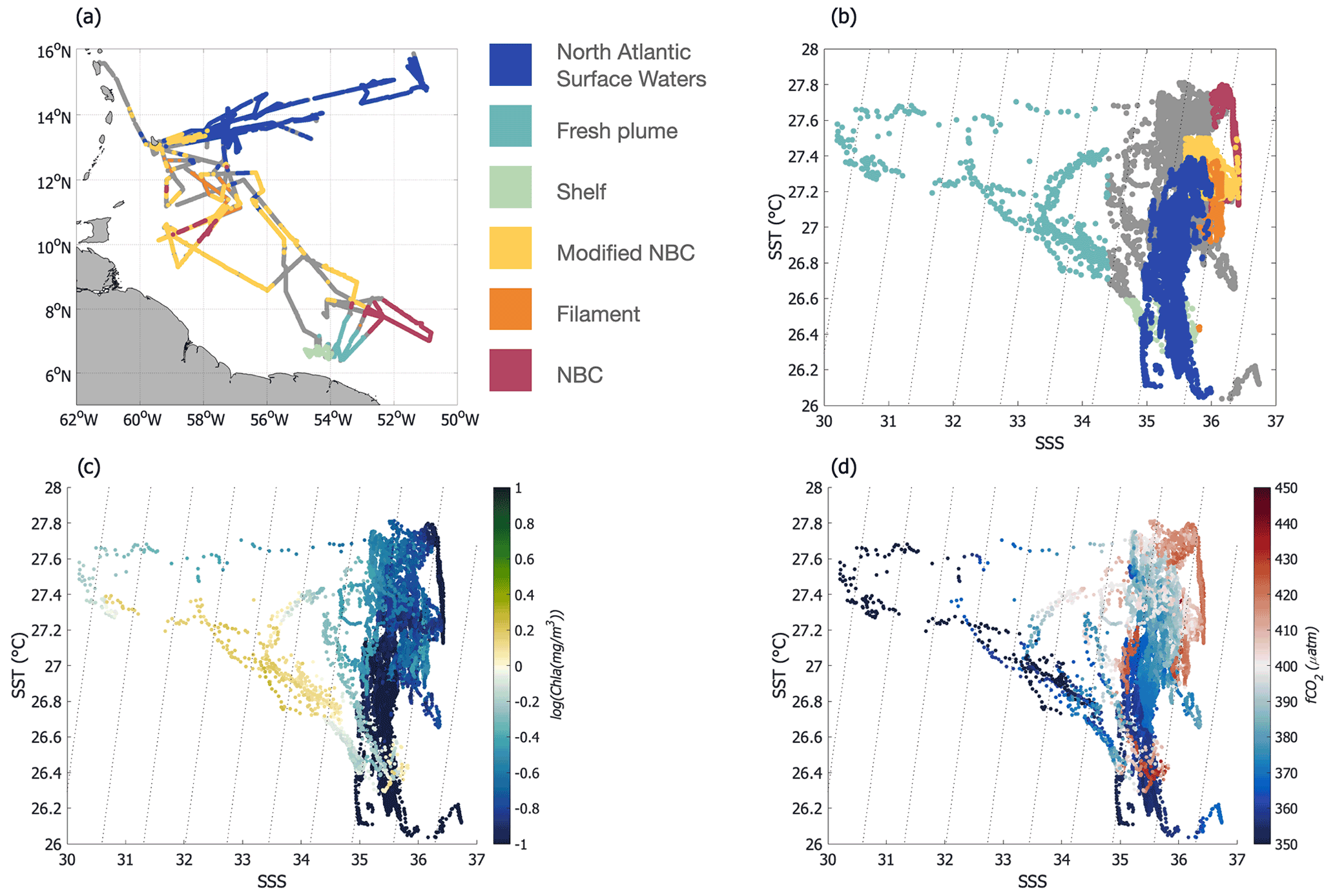
Figure 5 (a) Map representing Atalante, Merian and Ron Brown ship tracks colour-coded with the identified water masses. (b) T–S diagram colour-coded with the water masses; the grey colour corresponds to points that do not fit into the definition of the identified water masses.

North of Barbados, the domain is mostly dominated by North Atlantic Subtropical Waters (NASW), similar to Longhurst's NATR. They have a SSS in the range of 35 to 36 and are relatively cold (Table 1). Their SST diminishes over time towards the end of February. These waters are less influenced by coastal dynamics and therefore are not very productive at the surface (chl a levels inferior to 0.14 mg m⁻³) due to low nutrient levels. They are mainly located north of 13^∘ N and get progressively colder toward the northeast. RV Ron Brown stayed in that Trade Wind region for almost a month (Fig. 5). The observations collected from this ship show lower fCO₂ in NASW with respect to the atmosphere ($\mathrm{\Delta }f{\mathrm{CO}}_{\mathrm{2}}\sim -\mathrm{40}\mathrm{\mu }\mathrm{atm}$). Similar results are found on one of RV Merian's transects, with $\mathrm{\Delta }f{\mathrm{CO}}_{\mathrm{2}}<-\mathrm{30}$ µatm.

Table 1 Thresholds in SSS, SST and chl a used to define the six water masses identified in the winter WTA.

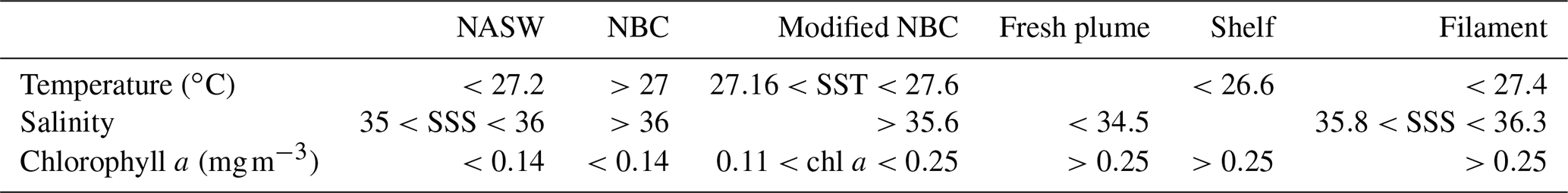
The NBC is surface-intensified and fed by the central branch of the South Equatorial Current (SEC; Schott et al., 1998). As the cold and saline water from the upwelling region is transported westward by the SEC, it warms up (SST>27 ^∘C) but retains its saline characteristic (SSS>36, Table 1) as it reaches the NBC retroflection region (Fig. 4). This NBC water mass is oligotrophic (Fig. 3b) and therefore in our area of interest distinguished itself by its low level of surface chl a (chl a<0.14 mg m⁻³). These waters are found in the retroflection area and were sampled by both RVs Merian and Atalante at the beginning of February (Fig. 5). The NBC water mass is in some way similar to the WTRA but does not extend beyond the retroflection, therefore representing a more limited part of the WTRA. We will introduce four new water masses in the following parts, as well as their associated dynamical structures. They can be considered as subsets of the WTRA and Guiana Coastal provinces, these two provinces being too large and not well suited to represent small-scale processes.

3.3 North Brazil Current rings

The extension of the NBC retroflection varies depending on the state of eddy formation. It moves northwestward up until 9^∘ N as an eddy is forming and then retracts to the southeastern part of the region. During our period of interest, the retroflection shed anticyclone A1 at the beginning of February. It is difficult to estimate the date of shedding as the area is highly dynamic, and detecting the first closed contour of ADT is complicated and may be inaccurate. It is however interesting that the two ships sampled the retroflection when it was expanding to generate A1, and this northwestward expansion is well observed on several physical and biogeochemical parameters (Fig. 7a). RV Merian crossed the retroflection on 27 January and stayed in the area until 2 February (Fig. 6). Chl a present on the shelf is advected by the strong currents on the periphery of the retroflection and delineates well its southwestern side (Fig. 7a). The NBC waters stand out on the surface T–S diagram as they are the most saline waters observed in the region (Fig. 7b). They are also high in fCO₂ which reflects their equatorial origin. Their SST is relatively warm, varying from 27.8 ^∘C at the crossing of the first retroflection front to 27.2 ^∘C. The region is rather homogeneous, with an almost constant SSS of 36.3 and ΔfCO₂ along the multiple crossings, as observed on the Merian and Atalante transects (Fig. 6). On average along those transects, the NBC fCO₂ is higher than fCO_2atm by 20 µatm.

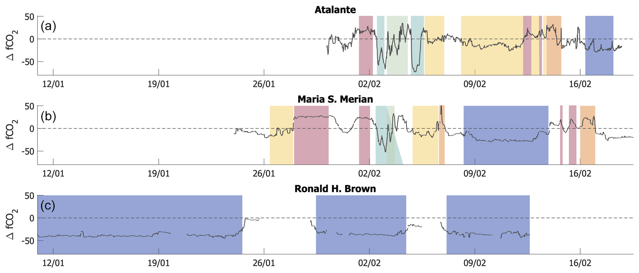
Figure 6 RVs Atalante (a), Merian (b) and Ron Brown (c) ΔfCO₂ time series. The background colour indicates the crossed water mass domains (see definition in legend of Fig. 5).

Anticyclone A1 is further crossed by RV Atalante on 6 February, just a few days after its separation from the retroflection (Fig. 7c). The surface signal is almost lost, both in SST and in fCO₂ (Fig. 7c and d). It is mainly composed of modified NBC water, whose properties are close to the NBC water (high SSS, high SST, low chl a) but not as pronounced. This water mass covers a larger area, which mainly encompasses the Eddy Boulevard region. It is defined here as SSS>35.6, $\mathrm{27.16}{}^{\circ }\mathrm{C}<\text{SST}<\mathrm{27.6}{}^{\circ }\mathrm{C}$ and $\mathrm{0.11}\mathrm{mg}{\mathrm{m}}^{-\mathrm{3}}<\text{chl}a<\mathrm{0.25}$ mg m⁻³ (Table 1). While the high chl a water delimits well the retroflection area, it partly covers eddy A1.

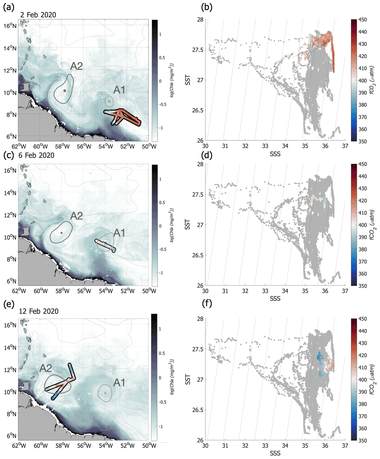
Figure 7 (a) RVs Atalante and Merian ship tracks in the NBC retroflection (Merian: 27 January to 2 February; Atalante: 2 February), (c) in NBC ring A1 (Atalante: 6 February) and (e) in NBC ring A2 (Atalante: 12–13 February; Merian: 13–14 February) colour-coded with fCO₂. The background represents the chl a on 2 (a), 6 (c) and 12 February (e), and the contours of NBC rings A1 and A2 are indicated. (b, d and f) Corresponding T–S diagrams colour-coded with fCO₂.

NBC ring A2 presents a different situation. Detached from the retroflection in early December 2019 (as defined from altimetry detection), it travelled northwestward while retaining an intense coherent core. Coastal waters identified by their high chl a content were less present and mostly entrained at the northwestward edge of the eddy. After 2 months, A2 almost reached Trinidad and Tobago and was located around 11^∘ N, 58^∘ W when it was sampled by the two ships (Fig. 7e). The SST signal is eroded, and most of the eddy is mostly made of modified NBC water with relatively low fCO₂. However, high SSS (36.5) and fCO₂ (415 µatm) are still visible near the eddy centre on the two crossings made by RV Atalante on 12 and 13 February. This is confirmed by the two sections of the Merian that crossed the altimetric eddy centre and measured SSS at 0.5 higher in the 50 km radius around the centre and above 36. The NBC water mass is therefore found close to the centre of eddy A2, as well as its associated high fCO₂.

From the collected observations, it appears that the surface signature of NBC rings is relatively variable and complex. It is well marked in their formation area in the NBC retroflection, where waters brought north by the NBC are warmer, saltier and higher in fCO₂ than the water of the northwestern tropical Atlantic. As the eddies travel northwestward, further away from the retroflection, they may be subject to various processes that modify the surface signal. Unfortunately, the data collected are not sufficient to shed light on which processes are involved in this situation. South of Barbados, away from the retroflection, the modified NBC is therefore the most common water mass. Nevertheless, the NBC water is still sometimes observed months after the separation from the retroflection in the eddy centre.

3.4 Freshwater plume

The NBC rings form and evolve in an area highly influenced by the Amazon River plume. Even if February is a period of low Amazon River outflow (Dai and Trenberth, 2002), freshwater events are relatively common. In February 2020, a freshwater plume detached from the Guiana plateau and spread out into the northwestern tropical Atlantic. The off-shelf plume was steered northward by the retroflection and NBC ring A1 up to 12^∘ N and then extended westward toward the Caribbean Sea. Waters carried by the plume strongly contrast with the saline waters of the retroflection. They include water from the Amazon and present low SSS (SSS<34.5), low fCO₂ (fCO₂<380 µatm) and high chl a (Table 1). The plume was crossed three times: twice on 2 February and once on 5 February (Fig. 6). Freshwater from the Amazon arrived on the plateau on 1–2 February and was then entrained northwestward by Ekman transport and geostrophic currents (Reverdin et al., 2021). On 2 February RVs Atalante and Merian left the retroflection area to cross the adjacent nascent plume. SSS rapidly decreased, reaching 33, which is associated with a strong decrease in fCO₂ (Fig. 8). From 2 to 5 February, the plume formed, and on 5 February the plume was approximately 100 km wide, with the lowest salinities around 30. Based on satellite SSS data of the following days, the plume appears to have reached even lower salinities and then spread out over the northwestern tropical Atlantic. It first spread northward, steered by A1, and then northwestward, channelled between A1 and A2 and reaching all the way up to 12^∘ N and extending over more than 100 000 km² (Reverdin et al., 2021). The plume can be followed by satellite SSS and chl a maps (Fig. 7a, c and e). Indeed, the low SSS is also accompanied by high chl a as water from the Amazon is considered highly productive. The northwestern tropical Atlantic is in general nutrient-limited, but the nutrients brought by the Amazon can support the occurrence of a bloom. The plume is also characterized by high silicate (between 4 and 10 µmol kg⁻¹ in the plume, almost 0 elsewhere), while nitrate and phosphate are rapidly consumed. Traces of inorganic phosphorus were observed in the plume, while nitrates were absent from surface waters (Fig. S2 in the Supplement). Low salinity combined with high biological productivity led to low fCO₂ and a strong carbon drawdown in the plume as the ΔfCO₂ reached −73 µatm on 5 February (Fig. 6).

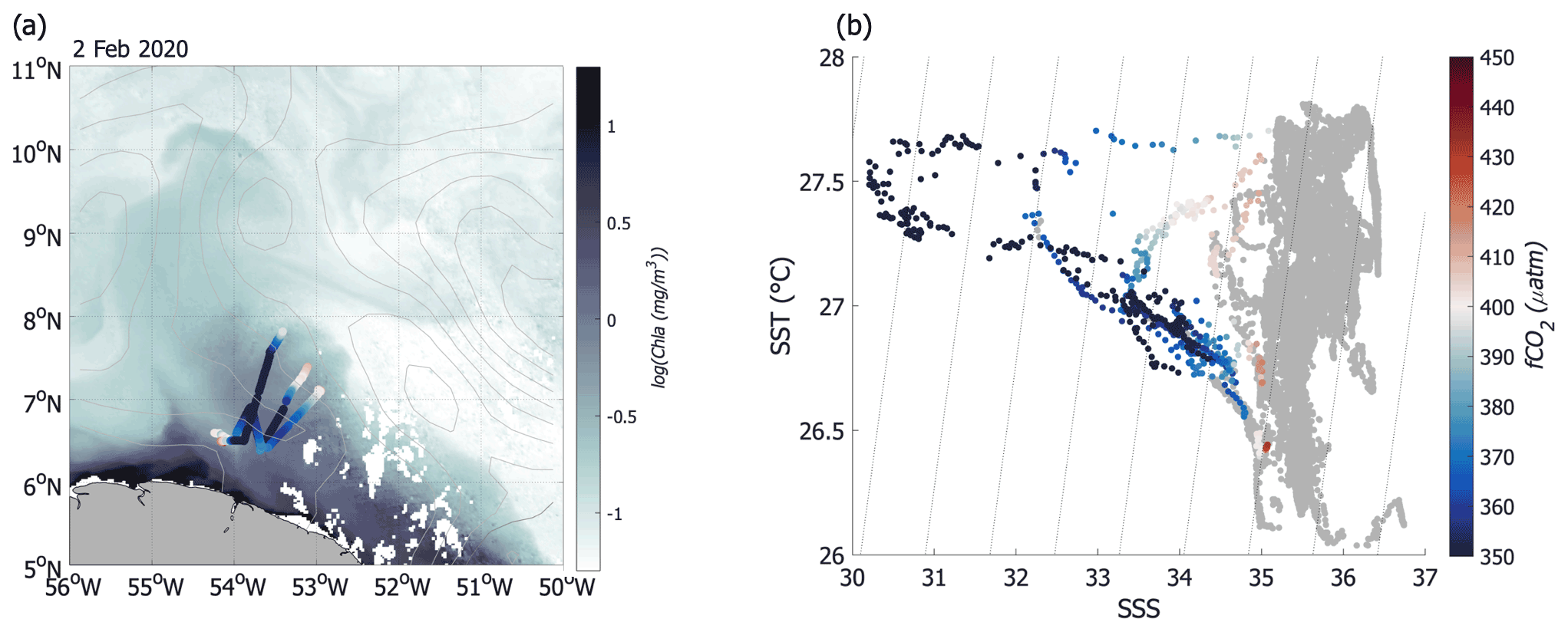
Figure 8 (a) RVs Atalante and Merian ship tracks in the freshwater plume (Atalante: 2 and 5 February; Merian: 2 February) colour-coded with fCO₂. The background represents the chl a on 2 February. (b) Corresponding T–S diagram colour-coded with fCO₂.

In an area highly influenced by the NBC waters, through rings or the retroflection, the plume stands out and modifies the biogeochemical dynamics of the region.

3.5 Shelf water and filaments

The freshwater plume is not the only water stirred by the NBC rings travelling from the NBC retroflection towards the Lesser Antilles. The shelf water is very different from the plume water and was only sampled sparsely on the way in and out of the plume (Figs. 4 and 5). On the Guiana plateau water is very rich in chl a and detrital material, rather saline (SSS∼35.5), and relatively cold (SST∼26.5 ^∘C) (Fig. 5 and Table 1). Since the water sampled on the edge of the plume was cold due to a local upwelling event (and/or vertical mixing event) detailed in the Supplement (Fig. S3 in the Supplement), temperature is not homogenous on the shelf.

Further north, a filament is stirred on the western side of NBC ring A2 (Fig. 9a). It is a small-scale structure, approximately 10 km wide and easily identifiable due to its high chl a. The filament is continuously stirred by A2 and so is already visible on chl a maps on 2 February (Fig. 7). It followed A2's westward translation and was crossed on 6 and 17 February by RV Merian and on 14 February by RV Atalante (Fig. 6). It has a SSS close to 36 and an SST between 27 and 27.5 ^∘C; thus, it is slightly colder and more saline than its surrounding waters (Fig. 9b and Table 1). It stands out because of its high chl a content (chl a>0.25 mg m⁻³) even if this is lower than close to the coast or in the freshwater plume. The strongest signal is observed on the ocean carbon parameters. In contrast to the freshwater plume, this filament presents very high fCO₂ (>430 µatm), highlighting different origins. It stands out from the ship track time series by also having a larger positive ΔfCO₂ (50 µatm). Whereas the freshwater plume observed more southeastward carries water recently arrived on the plateau from the Amazon, the northwestward filament contains shelf waters.

3.6 Air–sea CO₂ flux

In order to better characterize the impact of each structure on the regional flux, we computed air–sea CO₂ flux maps from satellite data, at a resolution of 2.5 km (Fig. 10), averaged over the period of the cruise (2–19 February). The along-track flux represented in Fig. 10a and the reconstructed regional field (Fig. 10b) show the importance of the small-scale dynamical structures and highlight two strong regimes that are found on the reconstructed map. The air–sea CO₂ flux in the northeastern part of the domain, characterized by the NASW, is mainly dominated by temperature effects, while further south the presence of NBC rings and their interactions with coastal waters create a strong dependence of the CO₂ flux on SSS and on the biological and biogeochemical processes highlighted by the chl a.

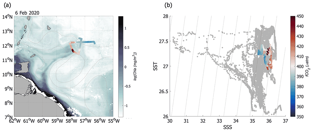
Figure 9 (a) RV Merian ship track in the shelf water filament (6 February) colour-coded with fCO₂. The background represents the chl a on 6 February. (b) Corresponding T–S diagram colour-coded with fCO₂.

We evaluate the integrated air–sea CO₂ flux over the region. In February, waters are the coldest, and the region is a strong CO₂ sink of −1.7 Tg C pr month (Fig. 11). Three biogeochemical domains mainly contribute to the air–sea CO₂ flux: the NASW, the freshwater plume and the NBC retroflection. The impact on the flux of the small-scale coastal filament is evident along the ship tracks (Fig. 10b). However, its contribution to the total flux is weak as the signal is smoothed when averaging over 2–19 February as the filament moves following the A2 ring's northwestward translation. Each of the main three regions is identified based on its averaged SST, SSS and chl a properties in February, and the region-specific flux is determined (Fig. 11).

NASW contributes about 60 % of the total sink due to the relatively cold temperature and to strong winds that enhance the air–sea exchanges. These waters extend from Barbados northward and eastward, cover more than one third of the domain, and show a weak variability over 2–19 February.

The NBC retroflection is a source of CO₂ to the atmosphere. In February, the strongest signal is observed in the southeastern part of the domain up to 8^∘ N, 53^∘ W. The retroflection nevertheless impacts the region as far as 10^∘ N, 54^∘ W as it is spatially variable, reaching up to 10^∘ N when shedding an eddy. The two NBC rings present a small positive February air–sea CO₂ flux average. Eddy A1 is almost stationary from its formation date (around 6 February) until 20 February, and its neutral to slightly positive CO₂ flux is centred around 10^∘ N, 54.5^∘ W (Fig. 10). Eddy A2 translates rapidly westward at the beginning of February and then northward from 15 February. Its signal is therefore not as visible as on the ship tracks as it is averaged over 19 d. The retroflection is the main region with a positive air–sea CO₂ flux; even if the region is too small to have a big global impact, understanding small-scale features may be significant for the total flux. The NBC rings carry part of the signal, which is heavily modified as they travel northwestward. As a result, on average in early to late February only the retroflection maintains a positive flux, while a large part of the domain dominated by modified NBC waters (not influenced by the plume) behaves as a small sink.

The freshwater plume with Amazon water is nascent when crossed by the ships (Fig. 10b) but is already the strongest signal of the time series. As the plume develops, it is entrained by NBC ring A1, then A2, and spreads out into the open ocean, as observed on SSS and chl a maps. The plume generates a strong CO₂ sink that is amplified by strong winds and reaches up to 12^∘ N (Fig. 10). The freshwater plume covers only 10 % of the total area but contributes to almost 20 % of the sink. In winter, this region either is not characterized in previous studies or is considered as dominated by high fCO₂ waters brought by the NBC to the climatology. We observe here that the trapping of CO₂-rich water by the NBC ring effect is relatively weak in winter, and the main signal is associated with the filaments they stir.

The northwestern tropical Atlantic therefore behaves as a sink of CO₂ in early to mid-February, driven by the cold North Atlantic subtropical waters and the Amazon freshwater plume stirred by NBC rings.

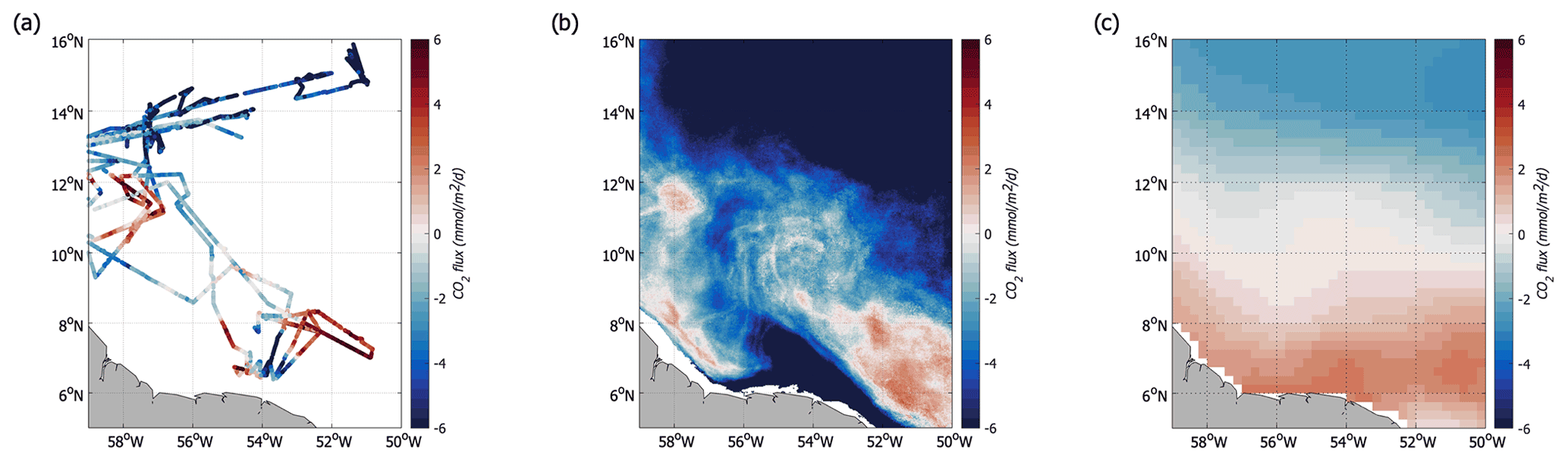
Figure 10 (a) Air–sea CO₂ flux measured in January–February 2020 during the EUREC⁴A-OA/ATOMIC cruise. (b) Air–sea CO₂ flux reconstructed over February 2020. (c) February climatology of the air–sea CO₂ flux over 1998–2015 (Landschützer et al., 2020).

4 Discussion

4.1 Integrated air–sea CO₂ flux

The northwestern tropical Atlantic presents a strong seasonal variability in air–sea CO₂ fluxes (Landschützer et al., 2016). In February, waters are the coldest, and we estimate the 5–16^∘ N, 59–50^∘ W domain to be a strong CO₂ sink of −1.7 Tg C per month (Fig. 11). This region, located at tropical latitudes but combining characteristics of subtropical waters and river outflow, is difficult to represent in large-scale climatologies. Indeed, the sink for the month of February is smaller by a factor of 10 in Landschützer et al. (2020) and is also considerably smaller in Takahashi et al. (2009), but the low spatial resolution of this last product does not allow for a good quantitative comparison. This region has been rarely observed, and the inter-annual variability described in Landschützer et al.'s (2020) climatology is therefore rather uncertain. The compensating effect of different years cannot explain entirely the difference of signal observed in February 2020 with respect to the two climatologies.

Three water masses mainly contribute to the air–sea CO₂ flux: the NASW, the fresh plume and the NBC retroflection. The NASW contributes about 60 % of the total sink and is not well captured in climatologies, with noticeable differences of more than 20 µatm between the measured ΔfCO₂ in 2020 and the one computed from Landschützer et al. (2020) and Takahashi et al. (2009) (the closest grid point is considered for this comparison). The retroflection is the main region with a positive air–sea CO₂ flux. Its influence is observed up to 10^∘ N, 55^∘ W, but its area is small, so its impact on the regional flux is weak. The positive flux of the retroflection is slightly overestimated in the climatologies, but it could also be due to the difficulty to detect the retroflection at the beginning of February. The main difference is that the NBC waters rich in CO₂ are localized in the retroflection area and are heavily modified when spreading into the Eddy Boulevard.

The freshwater plume is a feature previously not well described for this region in winter, and we found a contribution of almost 20 % to the sink. The impact of the Amazon River has been overlooked so far in winter, but it accounts for a large part of the salinity and biogeochemical variability. Freshwater from the Amazon is not just located on the shelf, but it can spread northward, advected by the strong current variability associated with the NBC rings (Reverdin et al., 2021). These rings are the largest, faster rotating and the most energetic during boreal winter compared to other seasons (Aroucha et al., 2020). Combined with a seasonal increase in the Amazon's outflow, it induces a large variability in SSS, chl a and fCO₂. The occurrence of freshwater export from the shelf to the open ocean has a strong influence on the salinity and therefore on the mixed layer depth and air–sea heat exchanges (Reverdin et al., 2021). It also strongly impacts the biogeochemistry of the region as the low fCO₂ is due both to the low salinity of the plume waters and to the biological activity. The plume stirred into the open ocean by the NBC rings brings nutrients in a region strongly nutrient-limited and generates a local winter bloom. This in turn plays an important role in the air–sea CO₂ flux and is a crucial feature of the southern part of the northwestern tropical Atlantic.

4.2 Extension to other years and inter-annual variability

Few tropical Atlantic measurements of biogeochemical tracers are available, in particular in the northwestern tropical Atlantic. The EUREC⁴A-OA/ATOMIC campaign provides the first in situ comprehensive measurements of fCO₂ in this region for the boreal winter season. The reconstruction of fCO₂ maps likely provides a good understanding of the spatial evolution of fCO₂ and air–sea CO₂ fluxes and is fitted for the months of January–February 2020. Although the processes described here are specific to winter and thus cannot be extended to other seasons, they will be useful to understand the winter variability in other years.

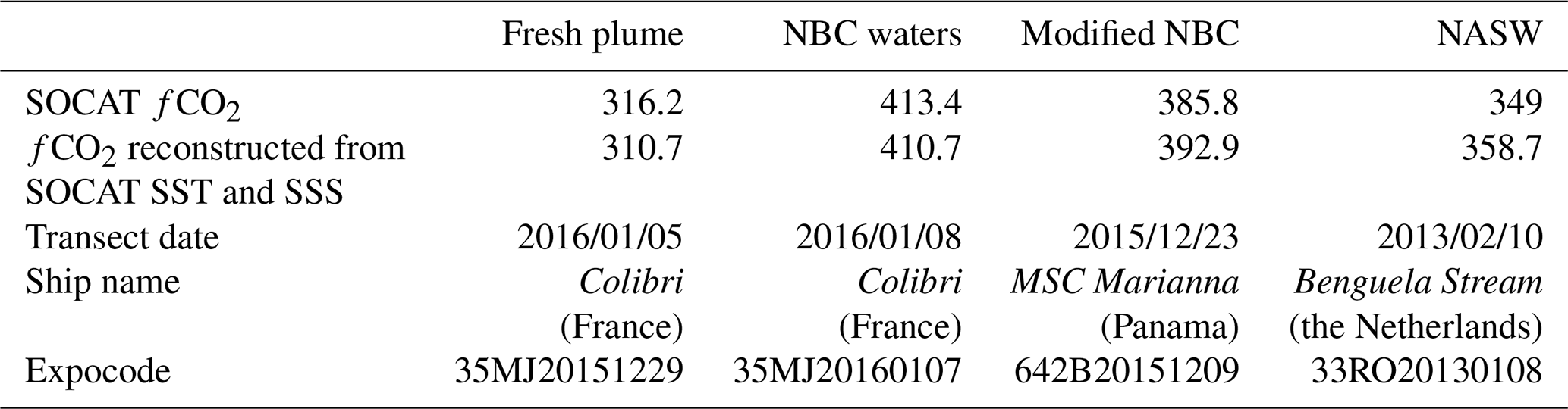
Only a few cruises crossed the region according to the SOCAT database between 2010 and 2019 (period with satellite SSS data), and investigating inter-annual variability is not possible. However, we can test the relation developed for 2020 for other years by using selected cruises from the SOCAT database. We thus first use the relationship to reconstruct fCO₂ along the ship tracks (using in situ SSS and SST and colocalized chl a) and then over the whole region based on satellite products (OSTIA (Operational Sea Surface Temperature and Sea Ice Analysis) SST, GlobColour chl a, CCI+SSS (Climate Change Initiative Sea Surface Salinity), detailed in Appendix A). A comparison between the measured and reconstructed fCO₂ for the water masses sampled by the SOCAT cruises (NASW, fresh plume, NBC retroflection, modified NBC) is presented in the appendix (Table A1). Good agreement is found between the fCO₂ from the SOCAT database and the one reconstructed from the in situ temperature and salinity, as well as co-localized chl a for the four water masses (averaged difference of 5.5 µatm). When comparing reconstructed fCO₂ maps with fCO₂ on ship tracks (Fig. A1), the agreement between fCO₂ in various water masses is very clear even though the spatial structures are sometimes a bit misplaced. This is attributable to the slightly coarser resolution of satellite products not designed specifically for each campaign, to the high spatio-temporal variability in fCO₂, and to missing chl a and SST observations in cloudy areas. February 2020 was mainly cloud free, so we were able to use high-resolution daily SST and chl a. The SSS product used in 2020 is also a daily product. However, for the other years, the satellite chl a (if clouds) and SSS products have a weekly temporal resolution which smears the fast-moving structures. The gradients between water masses are therefore not always well represented, but we find a good agreement between the fCO₂ of each structure, which is encouraging for future studies on inter-annual variability in winter.

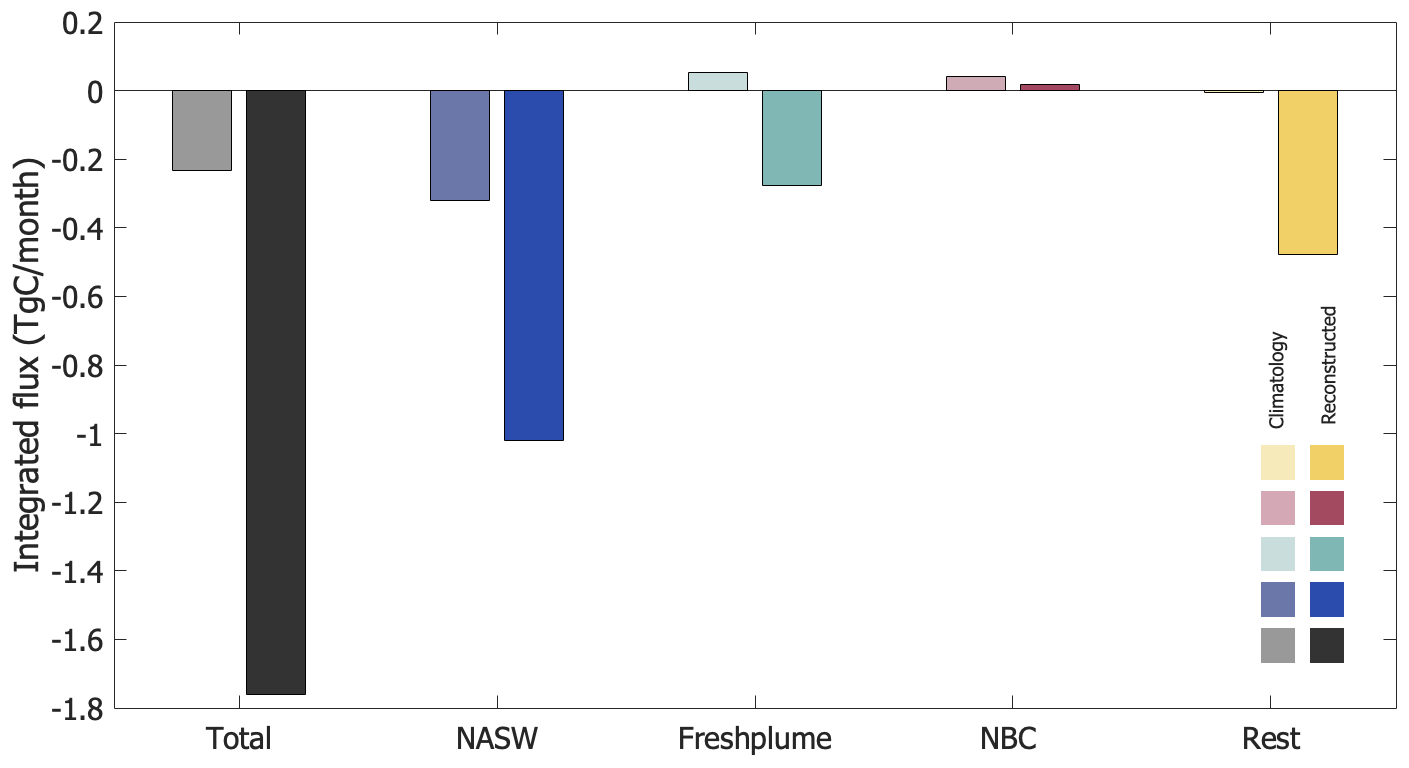
Figure 11 Integrated flux for the (5–16^∘ N, 59–50^∘ W) domain and for three water masses. For each bar duet, the one on the left in faded colours represents the integrated flux from Landschützer et al.'s (2020) February climatology, while the one on the right is computed from the reconstructed flux. Same colour code as in Fig. 5.

By identifying the main processes responsible for the variability in the air–sea CO₂ flux in 2020, we can better understand the inter-annual variability in the region. Indeed, each of the main water masses has its own inter-annual variability that shapes the CO₂ variability. The northern part of the domain is dominated by the variation in temperature, and therefore its inter-annual variability is mainly linked to the one of SST. From 32 years of monthly mean SST data, the SST standard deviation in the area is relatively weak and does not exceed 0.5 ^∘C. The northern sink of CO₂ is therefore rather similar from year to year, coherent with the low standard deviation of the air–sea CO₂ flux computed from Landschützer et al. (2020). Some variability is still observed in the snapshot of the reconstructed fCO₂ (Fig. 12) but to a much smaller extent than south of Barbados. For example, the strong sink observed in March 2014 is caused by cold SST anomalies over the whole domain. Some small-scale variability in the northern part of the domain is sometimes correlated to SSS anomalies, as in 2019.

The freshwater plume sampled during EUREC⁴A-OA is a common feature in February. During the 2010–2019 period, events of freshwater reaching the open ocean were observed each year, and freshwater plumes similar to the one described in this paper were observed during 7 out of 10 years of satellite salinity data (Reverdin et al., 2021). Two of the main mechanisms driving the occurrence of the plume are the winds near the Amazon estuary that can induce along-shelf transport to the Guyana plateau and the presence of NBC rings. Most of the plume events similar to the one in this study suggest the presence of an anticyclone to its east. This region is commonly crossed by several NBC rings during winter (Jochumsen et al., 2010; Johns et al., 2003; Mélice and Arnault, 2017), but it also is subject to a strong year-to-year variability that has linkages with the variability in the Amazon River outflow (Aroucha et al., 2020). Therefore, identifying and understanding the processes happening in 2020 should contribute to the better assessment of the inter-annual variability in fCO₂, as well as air–sea CO₂ fluxes, in the northwestern tropical Atlantic during winter. Using a combination of SSS, SST and chl a brings information on the biogeochemistry of the area in winter and represents well the mesoscale structure.

Figure 12 Snapshot of reconstructed fCO₂ for all occurrences of fresh plumes extending at least to 10^∘ N and east of 56^∘ W in January–March 2010–2019 (2010, 2011 and 2013 do not present this type of event).

5 Conclusions

The EUREC⁴A-OA/ATOMIC campaign provides for the first time synoptic measurements related to the air–sea fluxes of CO₂ in the northwestern tropical Atlantic in winter. Six main surface water masses are identified, one of them north of Barbados (North Atlantic Subtropical Water) and the other five (the NBC retroflection, modified NBC waters, the freshwater plume, the shelf water and the shelf filament) south of Barbados. The investigation highlights the two different regimes of the region. In the northern part, the variability in the CO₂ flux is low, and the area is covered by relatively cold, saline and low-chlorophyll NASW. The southern part is highly variable due to the presence of large mesoscale anticyclonic eddies. In January and February 2020, two NBC rings influence the physical and biogeochemical properties of the region. The NBC retroflection is characterized by waters with equatorial origins that are relatively warm, saline and high in fCO₂. As the rings separate from the retroflection, they interact with the surrounding waters, and the initial signal in fCO₂ is dampened. The main impact of the rings is therefore not necessarily on the surface water they transport in their core (eddy trapping) but rather on the filaments they stir off the coast (eddy stirring). A fresh plume from the Amazon River is transported by the coastal current up to the French Guiana shelf in the beginning of February. The NBC rings entrain the plume of freshwater up to 12^∘ N. This plume is fresh, rich in chl a, and low in fCO₂, strongly contrasts with the surrounding waters, and spreads over ∼100 000 km². On the shelf not influenced by the plume, water is relatively saline and high in fCO₂ and chl a probably due to a high concentration of detrital material. As ring A2 propagates westward, it continuously stirs a thin (10 km wide) filament of high fCO₂ shelf water up to 12^∘ N.

Based on the ship observations we identify distinct regimes in fCO₂ linked to certain combinations of SST, SSS and chl a properties. We use this information to construct high-resolution maps of fCO₂ and air–sea CO₂ flux using satellite maps of SSS, SST and chl a. On average over early to mid-February, the region acts as a strong sink of CO₂ (−1.7 Tg C per month), the sink being 10 times smaller in air–sea CO₂ flux climatologies. The NASW is responsible for most of the flux (60 %) due to low temperatures associated with winter cooling and strong winds. South of Barbados, the region also acts as a sink of CO₂. The influence of equatorial water is localized in the retroflection region that acts as a small source of CO₂. The main feature in this part of the domain is the fresh plume that contributes almost 20 % of the total sink.

The processes described here highlight the high variability in air–sea CO₂ fluxes in winter that are quite different from the ones in summer. These features are relatively common in winter and can be used to better understand the inter-annual variability in air–sea CO₂ fluxes. The northern part of the domain is driven by the variability in SST, while the southern one is a combination of the inter-annual variability in temperature, salinity and chlorophyll. It is therefore linked to the year-to-year variability in the NBC rings and the Amazon outflow.

This study is limited by the paucity of data in the region and for this time period. More fCO₂ data closer to the coast would help us to better quantify the influence of shelf water on the flux. The signature of the NBC rings has been described for only two rings that had different signatures. In order to reach more robust conclusions on the transport of surface NBC water by the rings, more eddies should be observed. The variability in fCO₂ occurs at large and small scales. Salinity is one of the most valuable predictors of fCO₂ south of 10^∘ N, but the satellite salinity resolution is much lower than those of temperature and chlorophyll. To have a more accurate prediction of the fCO₂, a high-resolution SSS product would also be very useful.

Appendix A

Due their long time series, the following SST, chl a and SSS products are used to reconstruct fCO₂ maps in winter in the northwestern tropical Atlantic for years other than 2020. Results are shown in Figs. A1 and 12. They are different than the satellite products used in the main study that were only available for a short period.

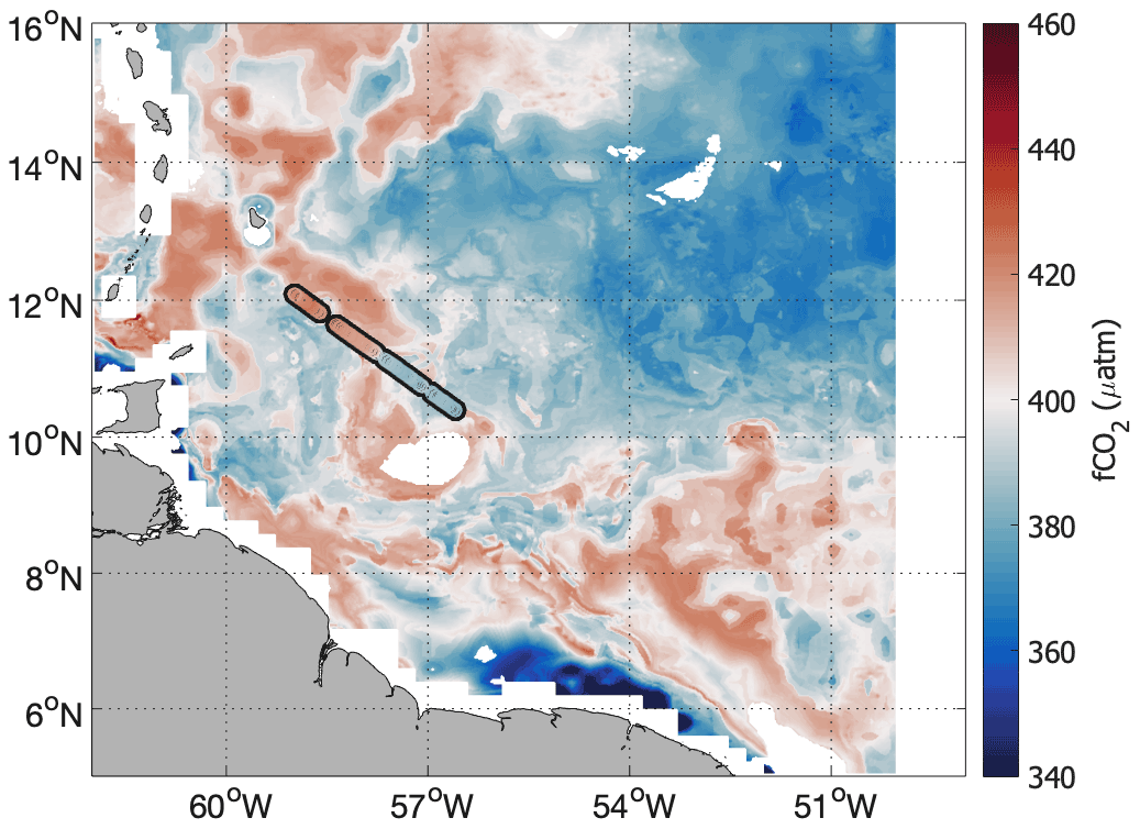
Figure A1 fCO₂ reconstructed from OSTIA SST, CCI+SSS and GlobColour chl a for 23 December 2015 superimposed with the fCO₂ from cruise 642B20151209.

Table A1 Comparison for the four main water masses between the fCO₂ from SOCAT transect and the fCO₂ reconstructed from in situ SSS and SST and colocalized chl a.

The OSTIA SST product, distributed by the Copernicus Marine Service (CMEMS) is used here. Daily maps of SST are produced at a resolution of $\mathrm{1}/\mathrm{20}$^∘ and are available from 1981 to present. OSTIA SST uses most SST data available for a day from both infrared and microwave inferred SST.

Surface chl a from GlobColour dataset derived from ocean colour at a $\mathrm{1}/\mathrm{24}$^∘ resolution is used. It is a merged product from multiple satellite missions' observations (SeaWiFS, MERIS, MODIS, VIIRS NPP, OLCI-A, VIIRS JPSS-1 and OLCI-B). GlobColour data are developed and validated by ACRI-ST and distributed by the CMEMS.

We also use SMOS and SMAP combined weekly SSS generated by the Climate Change Initiative Sea Surface Salinity (CCI+SSS) project (Boutin et al., 2021, https://doi.org/ 10.5285/5920a2c77e3c45339477acd31ce62c3c). It provides weekly level-3 SSS data from 2010 to 2019 at a spatial resolution of 50 km, sampled daily on a 25 km×25 km grid, by combining data from the SMOS, Aquarius and SMAP missions.