the Creative Commons Attribution 4.0 License.
the Creative Commons Attribution 4.0 License.
 | 21 Jul 2022
Benthic silicon cycling in the Arctic Barents Sea: a reaction–transport model study
James P. J. Ward
Katharine R. Hendry
Sandra Arndt
Johan C. Faust
Felipe S. Freitas
Sian F. Henley
Jeffrey W. Krause
Christian März
Allyson C. Tessin
Ruth L. Airs
Over recent decades the highest rates of water column warming and sea ice loss across the Arctic Ocean have been observed in the Barents Sea. These physical changes have resulted in rapid ecosystem adjustments, manifesting as a northward migration of temperate phytoplankton species at the expense of silica-based diatoms. These changes will potentially alter the composition of phytodetritus deposited at the seafloor, which acts as a biogeochemical reactor and is pivotal in the recycling of key nutrients, such as silicon (Si). To appreciate the sensitivity of the Barents Sea benthic system to the observed changes in surface primary production, there is a need to better understand this benthic–pelagic coupling. Stable Si isotopic compositions of sediment pore waters and the solid phase from three stations in the Barents Sea reveal a coupling of the iron (Fe) and Si cycles, the contemporaneous dissolution of lithogenic silicate minerals (LSi) alongside biogenic silica (BSi), and the potential for the reprecipitation of dissolved silicic acid (DSi) as authigenic clay minerals (AuSi). However, as reaction rates cannot be quantified from observational data alone, a mechanistic understanding of which factors control these processes is missing. Here, we employ reaction–transport modelling together with observational data to disentangle the reaction pathways controlling the cycling of Si within the seafloor. Processes such as the dissolution of BSi are active on multiple timescales, ranging from weeks to hundreds of years, which we are able to examine through steady state and transient model runs.
Steady state simulations show that 60 % to 98 % of the sediment pore water DSi pool may be sourced from the dissolution of LSi, while the isotopic composition is also strongly influenced by the desorption of Si from metal oxides, most likely Fe (oxyhydr)oxides (FeSi), as they reductively dissolve. Further, our model simulations indicate that between 2.9 % and 37 % of the DSi released into sediment pore waters is subsequently removed by a process that has a fractionation factor of approximately −2 ‰, most likely representing reprecipitation as AuSi. These observations are significant as the dissolution of LSi represents a source of new Si to the ocean DSi pool and precipitation of AuSi an additional sink, which could address imbalances in the current regional ocean Si budget. Lastly, transient modelling suggests that at least one-third of the total annual benthic DSi flux could be sourced from the dissolution of more reactive, diatom-derived BSi deposited after the surface water bloom at the marginal ice zone. This benthic–pelagic coupling will be subject to change with the continued northward migration of Atlantic phytoplankton species, the northward retreat of the marginal ice zone and the observed decline in the DSi inventory of the subpolar North Atlantic Ocean over the last 3 decades.
- Article
(4866 KB) - Full-text XML
-
Supplement
(2184 KB) - BibTeX
- EndNote


Diatoms are photosynthesising algae that take up dissolved silicic acid (DSi) from seawater to build silica-based frustules (termed “biogenic silica” (BSi) or “opal”), which are then recycled or reworked in transition to and within the seafloor. The seafloor acts as a biogeochemical reactor, generating a benthic return flux of DSi across the pan-Arctic region that is estimated to equal the input from all Arctic rivers (März et al., 2015). These recycling and reworking processes are therefore important for the regional silicon (Si) budget and for fuelling subsequent blooms, where seafloor-derived nutrients are able to be advected into the photic zone. Typically, Barents Sea phytoplankton spring blooms are dominated by diatoms (Wassmann et al., 1999; Orkney et al., 2020). However, temperate flagellate species are becoming more dominant in the Eurasian Basin of the Arctic Ocean and are expected to become the resident bloom formers in the region (Neukermans et al., 2018; Orkney et al., 2020; Oziel et al., 2020; Ingvaldsen et al., 2021). This shift in species composition is thought to be driven in part by an expansion of the Atlantic Water realm (“Atlantification”) (Fig. 1). Furthermore, nutrient concentrations in Atlantic Water flowing into the Barents Sea have declined over the last 3 decades and are forecast to do so throughout the 21st century (Neukermans et al., 2018, and references therein). Crucially, a much more significant drop in DSi concentrations has been observed relative to nitrate (Rey, 2012; Hátún et al., 2017), creating less favourable conditions for diatom growth (Neukermans et al., 2018).
This shift in phytoplankton community composition is predicted to reduce the export efficiency of phytodetritus, with potentially significant implications for pelagic–benthic coupling and thus the Si cycle (Fadeev et al., 2021; Wiedmann et al., 2020). Observations from long-term sediment trap data show that carbon export and aggregate sinking rates are 2-fold higher underneath diatom-rich blooms in seasonally sea-ice-covered areas of the Fram Strait, compared with that in Phaeocystis pouchetii-dominated blooms in the ice-free region (Fadeev et al., 2021). A similar contrast was observed in carbon export fluxes measured using short-term sediment trap deployments north of Svalbard (Dybwad et al., 2021). It is estimated that 40 %–96 % of surface ocean primary production is exported to the seafloor in the Barents Sea (Cochrane et al., 2009, and references therein), while the export efficiency of net primary production out of the euphotic zone in the central gyres is typically < 10 % (Turner, 2015, and references therein).
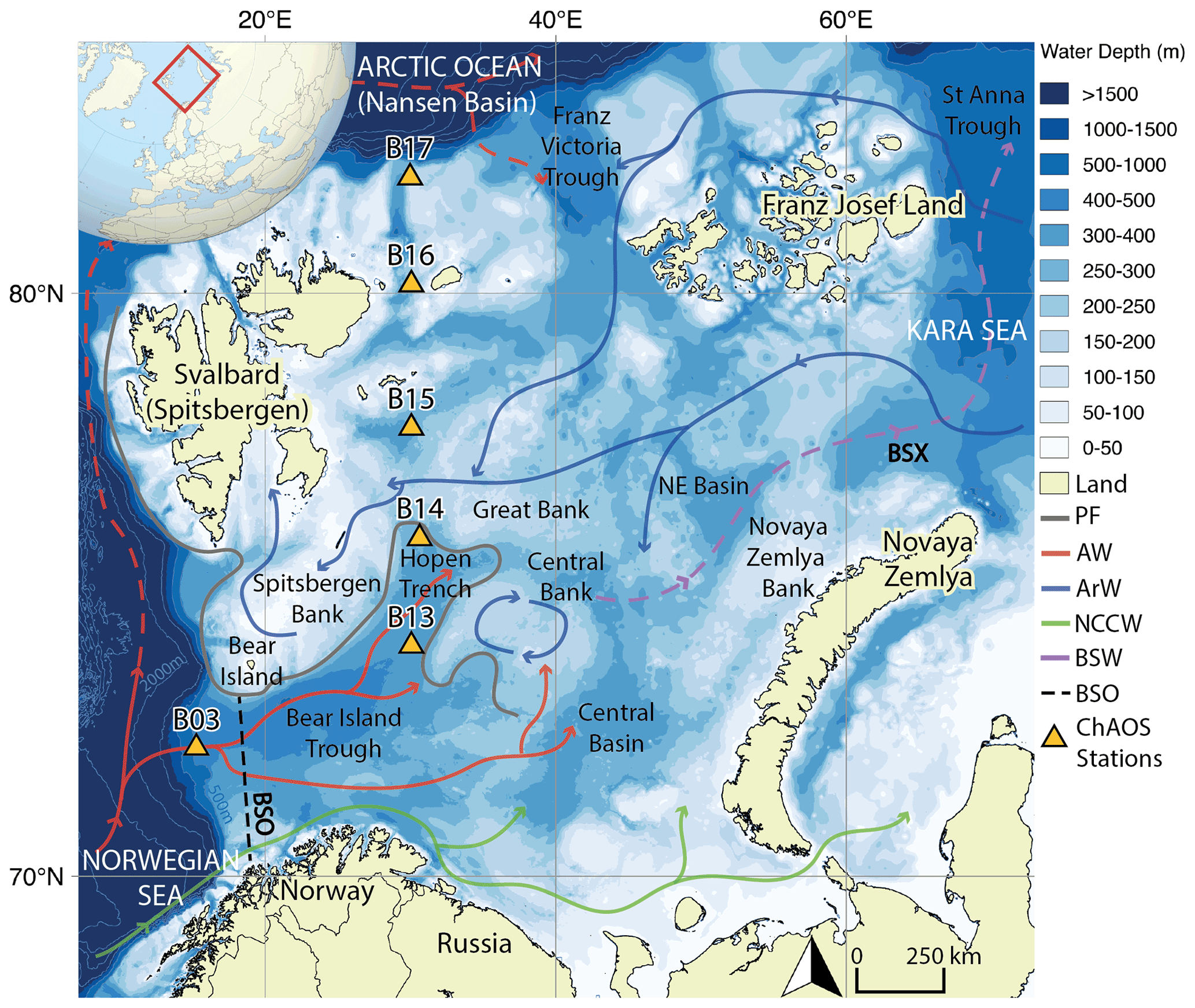
Figure 1Map of the Barents Sea shelf, including ChAOS stations, the main hydrographic features and water masses from Ward et al. (2022) (PF – oceanic polar front, AW – Atlantic Water, ArW – Arctic Water, NCCW – Norwegian Coastal Current Water, BSW – Barents Sea Water, BSO – Barents Sea Opening, BSX – Barents Sea Exit). Dashed red path refers to a subsurface water mass (Lien et al., 2013). High-resolution bathymetry data taken from the General Bathymetric Chart of the Oceans (GEBCO) (Jakobsson et al., 2012).
Given the changes forecast in the pelagic–benthic coupling of Si in the Arctic, it is important to understand the baseline benthic biogeochemical system in order to anticipate the implications of further perturbations. Based on Si isotopic data from various reactive sedimentary pools and the sediment pore water dissolved phase from the Barents Sea seafloor, Ward et al. (2022) hypothesised that the Si cycle is isotopically coupled to the redox cycling of metal oxides, most likely solid-phase Fe (oxyhydr)oxides. The reductive dissolution of Fe (oxyhydr)oxides and release of adsorbed Si (FeSi) are thought to drive marked shifts in the isotopic composition of the Barents Sea sediment pore water DSi pool towards lower values. Further, Ward et al. (2022) propose that sediment pore water undersaturation drives the contemporaneous dissolution of lithogenic silicate minerals (LSi) alongside BSi, some of which are reprecipitated as authigenic clay minerals (AuSi), representing a sink of isotopically light Si to the regional Si budget. Finally, Ward et al. (2022) propose that seasonal pelagic phytoplankton blooms generate stark peaks in pore water DSi that dissipate on the order of weeks to months. However, to fully understand the early diagenetic cycling of Si within the seafloor of the Barents Sea, we must be able to quantify the relative contribution of LSi and BSi to the DSi pool, as well as establish whether AuSi precipitation removes a significant portion of that pool. Here we employ steady state reaction–transport modelling to reconstruct the benthic cycling of Si in the Barents Sea, informed by our dataset of solid- and dissolved-phase Si isotopic compositions (Ward et al., 2022) to test these hypotheses. Such techniques allow for the disentangling and quantification of the aforementioned early diagenetic reactions (Geilert et al., 2020a; Ehlert et al., 2016a; Cassarino et al., 2020), as well as the return benthic flux of DSi to the overlying bottom water. Furthermore, reaction–transport modelling allows for the quantification of processes on much shorter timescales; thus we use transient model runs to validate the hypothesis that the pulsed deposition of bloom-derived BSi can perturb the benthic Si cycle. We then quantify the bloom-derived BSi contribution to the total annual benthic DSi flux, the deposition of which is subject to the anticipated shifts in community compositions of pelagic primary producers across the Arctic Ocean.
Understanding the key aims presented here not only is important for anticipating the biogeochemical response of the Barents Sea seafloor to physical, chemical and biological changes in the surface ocean but also has implications for the pan-Arctic Si budget. Currently there are disparities in the isotopic and mass balances of the Arctic Ocean Si budget, with Torres-Valdés et al. (2013) concluding that the Arctic Ocean is a slight net exporter of Si. Furthermore, a recent isotopic assessment identified the need for an additional benthic sink of light Si to close the Si budget (Brzezinski et al., 2021). However, current understanding is limited by a lack of direct observations from major gateways, including the Barents Sea (Brzezinski et al., 2021). By coupling observational data with reaction–transport modelling, we are able to construct a balanced Si budget for the Barents Sea (Sect. 3.5), contributing to the data gaps that currently limit our understanding of pan-Arctic Ocean Si cycling.
2.1 Oceanographic setting
The Barents Sea is one of seven shelf seas encircling the central Arctic Ocean and lies on the main inflow route for Atlantic Water. Oceanic circulation is driven by regional cyclonic atmospheric circulation and constrained by areas of prominent bathymetry (Fig. 1) (Smedsrud et al., 2013). Atlantic Water is fed in through the Barents Sea Opening between mainland Norway and Bear Island. This water mass then flows northwards, where it is met by colder, fresher Arctic Water, infiltrating the Barents Sea from the northern openings (Oziel et al., 2016). The oceanic polar front delineates these two water masses, the geographic position of which is tightly constrained in the western basin by the bathymetry but is less well defined in the east (Barton et al., 2018; Oziel et al., 2016). The heat content of the Atlantic Water-dominated region south of the polar front maintains a sea-ice-free state year-round, whereas the northern Arctic Water realm is seasonally sea-ice-covered, with a September minimum and a March/April maximum (Årthun et al., 2012; Faust et al., 2021).
The Barents Sea winter sea ice extent has been in decline since circa 1850 (Shapiro et al., 2003), but from 1998 the rate of retreat has become the most rapid observed on any Arctic shelf (Oziel et al., 2016; Årthun et al., 2012). Current forecasts suggest the Barents Sea will become the first year-round, sea-ice-free Arctic shelf by 2075 (± 28 years) (Onarheim and Årthun, 2017). The atmospheric and water column warming driving this sea ice retreat is a result of both anthropogenic and natural processes, with recent Atlantification arising from a northward expansion of the Atlantic Water realm (Årthun et al., 2012) and a reduction in sea ice import to the northern Barents Sea. The impact of these changes is an increase in upward heat fluxes, which inhibits sea ice formation (Lind et al., 2018).
The dynamic nature of the Barents Sea with respect to the physical oceanographic characteristics is reflected biologically in the ecosystems of the two main hydrographic realms. Annual primary production is estimated to range from 70 to 200 g C m−2, with lower values found in the northern Arctic Water realm, where a deep meltwater-formed pycnocline limits nutrient replenishment through wind-induced mixing (Sakshaug, 1997; Wassmann et al., 1999). However, the most distinct peaks in the rates of primary production are found in the marginal ice zone (MIZ) (reaching 1.5–2.5 g C m−2 d−1; Hodal and Kristiansen, 2008; Titov, 1995) (Fig. 2), which forms in spring/early summer as sea ice melts and retreats northwards, stratifying the water column and stabilising the nutrient-rich photic zone (Wassmann et al., 2006; Reigstad et al., 2002; Olli et al., 2002; Krause et al., 2018; Wassmann et al., 1999; Vernet et al., 1998; Wassmann and Reigstad, 2011). The phytoplankton communities of the Barents Sea in proximity to the polar front and MIZ tend to be dominated by pelagic and ice-associated diatom species, as well as the prymnesiophyte P. pouchetii (Syvertsen, 1991; Wassmann et al., 1999; Degerlund and Eilertsen, 2010; Makarevich et al., 2022).
2.2 Reaction–transport modelling
2.2.1 General approach
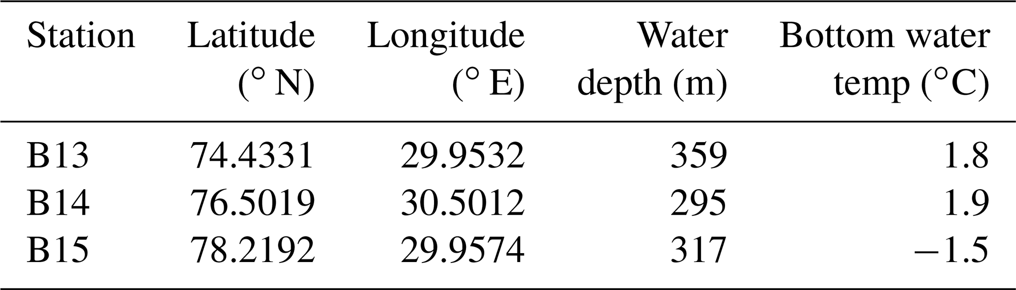
We use the Biogeochemical Reaction Network Simulator (BRNS) to disentangle the interplay of chemical and physical processes involved in the early diagenetic cycling of Si at stations B13, B14 and B15 of the Changing Arctic Ocean Seafloor (ChAOS) project in the Barents Sea (Figs. 1 and 2, Table 1). These stations span the main hydrographic features (polar front) and realms (Atlantic Water and Arctic Water) of the Barents Sea. BRNS is an adaptive simulation environment suitable for large, mixed kinetic–equilibrium reaction networks (Regnier et al., 2002, 2003; Aguilera et al., 2005), which is based on a vertically resolved mass conservation equation (Eq. 1) (Boudreau, 1997), simulating concentration changes for solid and dissolved species (i) in porous media at each depth interval and time step.
where ω, Ci, t and z represent the sedimentation rate, concentration of species i, time and depth respectively. The porosity term σ is given as for solid species and σ=φ for dissolved species, where φ is sediment porosity (Table S2). This term ensures that the respective concentrations represent the amount or mass per unit volume of sediment pore water or solids as required (Boudreau, 1997). Dbio is the bioturbation coefficient (cm2 yr−1) and was determined experimentally alongside this study (Solan et al., 2020). Di (cm2 yr−1) is the effective molecular diffusion coefficient (Di=0 for solids), and αi (yr−1) represents the bioirrigation rate (αi=0 for solids). Rj represents the rate of each reaction (j), and is its stoichiometric coefficient. A full description of the model can be found in Sect. S2 of the Supplement.
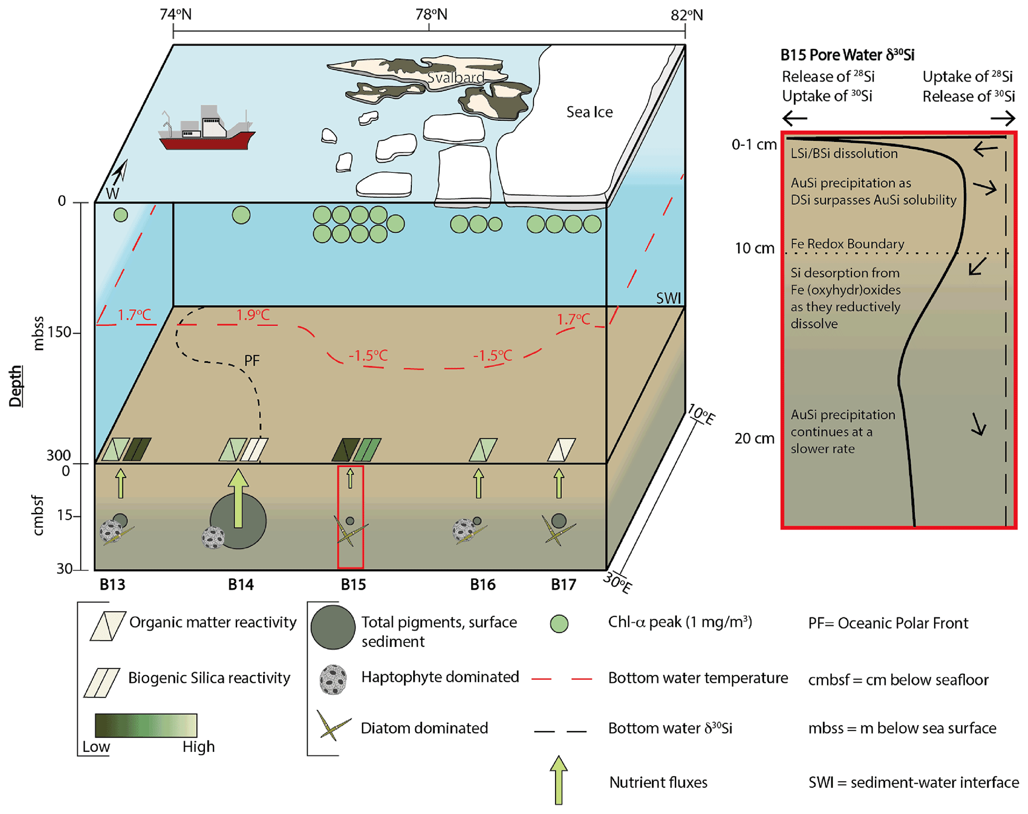
Figure 2Changing Arctic Ocean Seafloor (ChAOS) project summary. Chlorophyll α represents the peak value measured at each station during JR16006 CTD casts; data are available at https://www.bodc.ac.uk/data/published_data_library/catalogue/10.5285/89a3a6b8-7223-0b9c-e053-6c86abc0f15d/ (last access: 14 April 2022). Benthic nutrient flux magnitudes are for DSi measured in this study and Ward et al. (2022), as well as and from Freitas et al. (2020). The red box is a schematic summary of the main processes involved in the early diagenetic cycling of Si in the Barents Sea, derived from the results of the steady state model simulations in this study. Sea ice extent represents an approximation of the conditions at the time of sampling in 2017 and 2019. BSi reactivities were determined by the steady state model simulations. Please see Supplement Sect. S4 for a description of sediment pigment extraction methods. BSi – biogenic silica; LSi – lithogenic silica; AuSi – authigenic clay minerals; DSi – dissolved silicic acid.
2.2.2 Steady state reaction–transport modelling
Steady state modelling was employed to reproduce Si isotopic observational data in order to quantify the reaction rates of key processes involved in the cycling of Si within the seafloor. The version of the Si BRNS model employed here is adapted from Cassarino et al. (2020), which largely follows the approach of Ehlert et al. (2016a) and assumes a steady state. To ensure a steady state was achieved in the baseline simulations, the applied run time was dependent upon the sedimentation rate (0.05–0.06 cm yr−1; Zaborska et al., 2008; Faust et al., 2020) and core length so as to allow for at least two full deposition cycles (∼ 2500 years for a 50 cm Barents Sea core). The implemented reaction network accounts for a pool of pore water DSi, sourced by a dissolving BSi phase, from which Si can be incorporated into authigenic clay minerals (AuSi) as they precipitate. The kinetic rate law for the dissolution of BSi follows Eq. (2) (Hurd, 1972), where kdiss is the reaction rate constant (yr−1) and BSisol is the solubility of BSi (mol cm−3), implying that the rate of dissolution is proportional to the saturation state. The rate of BSi dissolution is allowed to decrease exponentially downcore in order to account for a reduction in reactivity due to BSi maturation and interaction with dissolved Al, as well as the preferential dissolution of more reactive material at shallower depths (Rickert, 2000; Van Cappellen and Qiu, 1997b; Rabouille et al., 1997; Dixit et al., 2001). The rate constants for BSi dissolution (kdiss, Eq. 2) were constrained using the solid-phase BSi content measurements (Fig. 3).
Equation (2) represents a simplification of the reaction rate law, which in reality is influenced by processes not incorporated into the model, such as surface area, temperature, pH, pressure and salinity. It is possible in some circumstances for the dissolution rate to deviate from the linear rate law (Van Cappellen et al., 2002); however, it is generally accepted that the dissolution of BSi is predominantly driven thermodynamically by the degree of undersaturation, leading to the linear rate law implemented in this study (Van Cappellen et al., 2002; Rimstidt and Barnes, 1980; Van Cappellen and Qiu, 1997b; Loucaides et al., 2012).
The precipitation of AuSi was modelled through Eq. (3), where kprecip is the precipitation rate constant (Ehlert et al., 2016a). This rate law assumes that the reaction will proceed, providing the concentration of DSi is greater than the solubility of the AuSi (AuSisol). The rate is thus proportional to the degree of pore water DSi oversaturation (Ehlert et al., 2016a). We assume a value of 50 µM for AuSisol at all three stations (Lerman et al., 1975; Hurd, 1973) (Table S2). As with BSi dissolution, the rate of AuSi precipitation was allowed to decrease exponentially with depth, compatible with the hypothesis that the majority of AuSi precipitation occurs in the upper portion of marine sediment cores. Here, DSi can more easily precipitate in the presence of more readily available dissolved Al, the concentration of which is typically higher in the upper reaches of shelf sediments, sourced from the dissolution of reactive LSi (e.g. feldspar and gibbsite) contemporaneously to that of BSi (Aller, 2014; Rabouille et al., 1997; Van Beusekom et al., 1997; Ehlert et al., 2016a).
In addition to the dissolution of BSi and precipitation of AuSi accounted for in previous early diagenetic modelling studies of the benthic Si cycle (Ehlert et al., 2016a; Cassarino et al., 2020), we incorporate the dissolution of LSi, which is thought to be an important oceanic source of numerous elements, including Si (Geilert et al., 2020a; Tréguer et al., 1995; Jeandel et al., 2011; Fabre et al., 2019; Ehlert et al., 2016b; Jeandel and Oelkers, 2015; Pickering et al., 2020; Morin et al., 2015). Here we assume that the dissolution of LSi is predominantly driven by the degree of undersaturation (Eq. 4), although as with the dissolution of BSi, LSi dissolution is a complex reaction and sensitive to processes that are not included in the model, including the potential for being catalysed by microbes (Vandevivere et al., 1994; Vorhies and Gaines, 2009; Liu et al., 2017). The undersaturation of Si minerals is known to include most primary and secondary silicates; thus dissolution extends beyond BSi in marine sediments (Isson and Planavsky, 2018, and references therein). Indeed, a suite of experiments have shown that primary silicates and clay minerals can rapidly release Si when placed in DSi-undersaturated seawater and take up Si in DSi-enriched waters (Siever, 1968; Mackenzie et al., 1967; Lerman et al., 1975; Hurd et al., 1979; Fanning and Schink, 1969; Mackenzie and Garrels, 1965; Gruber et al., 2019; Pickering, 2020). Lerman et al. (1975) determined in one such experiment that the dissolution of eight clay minerals could be described by a first-order reaction rate law driven by the saturation state, consistent with that applied here. Further, our assumption that LSi dissolution is driven by the degree of undersaturation is consistent with the suggestion that low bottom water DSi concentrations of the North Atlantic Ocean could allow for the dissolution of silicate minerals and thus account for high benthic DSi flux magnitudes in areas almost devoid of BSi (< 1 wt %) (Tréguer et al., 1995). A value of ∼ 100 µM was used for the solubility of LSi (LSisol) at all three stations, consistent with observations during multiple dissolution experiments of common silicate minerals in seawater (Table S3) as well as the estimated solubility of amorphous silica in high-detrital-component estuarine sediments (Kemp et al., 2021).
The desorption of Si from solid Fe (oxyhydr)oxide phases under anoxic conditions was simulated using a simple reaction rate constant (kFeSi), representing the rate of desorption. The value assigned to kFeSi was calculated during the modelling exercise, and no assumed amount of FeSi was included in the upper boundary conditions. This parameter likely represents a significant simplification; however the exact process pertaining to the adsorption of Si onto Fe (oxyhydr)oxides is unclear and requires further study (Geilert et al., 2020a). Step functions were included in the FeSi reactions in the model to simulate the desorption of this phase at specific depth intervals, representing the Fe redox boundaries identified in Ward et al. (2022). The step functions act as a cut-off mechanism, either setting reaction rates to zero or activating them at specific depths. A full description of the model, including all boundary conditions and how isotopic fractionation was imposed in the AuSi precipitation and FeSi desorption reactions, can be found in Sect. S2 of the Supplement.
Our estimates for all reaction rate constants in the steady state simulations (kdiss, kprecip, kLSidiss and kFeSi) were not based on published values and were model-derived (Table S2). These values were constrained by ensuring the best fit of the observational data with the simulated solid-phase BSi content and pore water DSi concentration and isotopic compositions, which were obtained by minimising the root-mean-square error (RMSE) between simulated and measured values (Table S1). Despite being model-derived, kdiss values (0.0055–0.074 yr−1) are found to lie within the published range for marine sediment BSi (Sect. 3.2). After the best-fit scenarios were established for each station, a sensitivity experiment was carried out by sequentially setting each reaction rate constant to zero in order to assess the importance of each process to the model fit (Fig. 3).
2.2.3 Processing the simulated data
Depth-integrated rates (R) of a given reaction (j) were calculated across the model domain using Eq. (5), for the best-fit simulation data of each station.
where L is the model domain length and dx denotes the given depth interval.
The deposition flux of BSi at the sediment–water interface (SWI) (JBSi,in) was then calculated based on Eq. (6), which states that JBSi,in equates to the sum of the flux of BSi out of the sediment (assumed to equate to the integrated rate of BSi dissolution, Rdb) and the BSi burial flux (JBSi,bur) (Burdige, 2006; Freitas et al., 2021). JBSi,bur was estimated at the base of the model domain (50.4 cm), following Eq. (7) on mass accumulation (Varkouhi and Wells, 2020, and references therein), which is controlled solely by advection. The sedimentation rate at depth (ωz) was corrected for compaction following Eq. (8) (Berner, 1980). JBSi,bur calculations assume a sediment wet bulk density of 1.7 g cm−3, consistent with previously assumed values for the Arctic seabed (Brzezinski et al., 2021; Backman et al., 2004) and that measured in clay-rich sediments of the Barents Sea (Orsi and Dunn, 1991).
We are also able to use the model simulation output to determine the total benthic flux of DSi at the SWI (Jtot), which has multiple constituent parts that contribute to the benthic flux magnitude. Following Eq. (9) (Freitas et al., 2020), we calculate Jtot and thus the relative contributions from bioturbation (Jbioturb), bioirrigation (Jbioirr), advection (Jadv) and molecular diffusion (Jdiff) to complement the calculated Jdiff estimates and core-incubation-derived Jtot of Ward et al. (2022).
2.2.4 Transient reaction–transport modelling
The influence of seasonality in pelagic primary production on the benthic Si cycle of the Barents Sea has been inferred through interpretation of pore water DSi depth profiles at station B14 (Ward et al., 2022). However, BRNS assumes a steady state and therefore cannot resolve seasonal biogeochemical dynamics without modification to allow certain boundary conditions to become time-dependent, enabling their activation and deactivation on a temporal scale. Here we use transient model runs to test the hypothesis that the pulsed deposition of bloom-derived BSi can rapidly perturb the benthic DSi pool, which is then able to recover on the order of weeks to months.
The steady state baseline simulations at station B14 represent a data–model best fit of the 2018 observational data, wherein we do not observe transient peaks in sediment pore water DSi concentrations (Fig. 4). This steady state scenario was used as the initial conditions for the transient simulations, which were run for 1 simulation year, producing output data at weekly time intervals. We simulate the phytoplankton spring bloom event by incorporating a step function to temporarily increase the BSi deposition flux and reactivity, simulating the effects of a 1- to 3-week spring bloom in late spring/early summer on the delivery of BSi to the seafloor. Durations of 1 and 3 weeks are thought to represent the typical length of a Barents Sea MIZ and spring bloom respectively (Sakshaug, 1997; Dalpadado et al., 2020) (Fig. 4). All boundary conditions were kept constant, with the exception of those related to the bloom-derived BSi pool.
During the 1- to 3-week time interval, the bloom-derived material was deposited at a rate equivalent to an increase in the steady state BSi deposition flux of 10- to 30-fold (Fig. 4). The background BSi deposition flux magnitude at station B14 is a model-derived parameter, constrained in the steady state simulations with the measured sediment BSi content and pore water DSi depth profiles. A 30-fold increase on the background deposition flux is similar to observations of a 10 d post-bloom diatom mass sinking event in the subpolar North Atlantic down to 750 m depth (26-fold increase) (Rynearson et al., 2013). The Barents Sea covers a relatively shallow continental shelf (average depth 230 m), and intense physical mixing at the polar front has been shown to enhance rates of vertical organic carbon flux at depth, close to station B14 (Wassmann and Olli, 2004). We could therefore anticipate an even greater increase in BSi depositional flux under bloom conditions than the maximum value assumed here. The reactivity of the bloom-derived material (kdissbloom) ranged from 5 to 20 yr−1, which is within the reactivity range of fresh pelagic BSi (3 to 100 yr−1; Ragueneau et al., 2000; Nelson and Brzezinski, 1997) (Fig. 4). Each of these three boundary conditions (length of the bloom period, kdissbloom and the deposition flux) was varied across multiple simulations within the constraints of published values to assess the influence of each parameter on the size and longevity of the sediment pore water DSi peak. The boundary conditions were determined to test whether peaks in pore water DSi concentrations are able to form within 1.5 months and dissipate within 3 months of the bloom, as proposed by Ward et al. (2022) and evidenced by contrasting sea ice conditions across the three cruises (Sect. 3.2; Fig. 4).
2.3 Observational data
As many reactions responsible for the biogeochemical cycling of Si between the solid and dissolved phases fractionate the isotopes of Si (28Si, 29Si, 30Si) relative to each other, we are able to use stable Si isotopes as a tool to trace these pathways. All solid-phase, core top and sediment pore water samples collected for Si isotopic analysis were collected over three summers in the Barents Sea (30∘ E transect spanning 74 to 81∘ N) aboard the RRS James Clark Ross (2017, 2018, 2019). Dissolved-phase pore and core top water DSi concentration measurements were determined on board using a Lachat QuikChem 8500 flow injection analyser with an accuracy of 2.8 %, defined using certified reference materials (CRMs; Kanso Technos Co., Ltd.). Stable Si isotopic compositions of the samples were determined at the University of Bristol in the Bristol Isotope Group laboratory. Isotopic compositions are expressed in δ30Si notation (per mille, ‰), relative to the international Si standard NBS-28 (Eq. 10). A full description of field methods, as well as Si isotopic and concentration data of the solid- and dissolved-phase reconstructed using BRNS, is provided in Ward et al. (2022).
Model upper boundary conditions for the dissolved phase were based on the DSi concentration and Si isotopic composition of the core top waters (+1.64 ± 0.19 (n=5), +1.46 ± 0.15 (n=3) and +1.69 ± 0.18 ‰ (n=6) at stations B13, B14 and B15 respectively). The Si isotopic compositions of the solid phases (BSi, LSi, FeSi) implemented in the model were determined based on a series of sequential digestion experiments carried out on surface sediment samples of the three aforementioned stations (Ward et al., 2022). The digestion sequence (0.1 M HCl, 0.1 M Na2CO3, 4 M NaOH) activates operationally defined reactive pools of Si, including Si-HCl (Si associated with metal oxide coatings on BSi, assumed here to represent the FeSi pool), Si-Alk (authigenically altered and unaltered BSi) and Si-NaOH (LSi and refractory BSi) (Pickering et al., 2020). The composition of the FeSi (−2.88 ± 0.17 ‰, n=20) and LSi (−0.89 ± 0.16 ‰, n=18) pools in Barents Sea sediment leachates was within long-term reproducibility of diatomite standard measurements (2σ ± 0.14 ‰, n=116) across the three stations, whereas the BSi phase was found to vary spatially, with an isotopic composition of +0.82 ± 0.16 ‰ (n=14) at station B15 and +1.43 ± 0.14 ‰ (n=8) and +1.50 ± 0.19 ‰ (n=7) at stations B13 and B14 respectively (Ward et al., 2022).
Table 1Sampling station information averaged across the three Changing Arctic Ocean Seafloor (ChAOS) cruises.
Gaining a better mechanistic understanding of benthic biogeochemical Si cycling in the Barents Sea is important to anticipate the effects of further natural and anthropogenically driven environmental perturbations, as well as to begin to address key knowledge gaps that currently limit our understanding of the pan-Arctic Ocean Si budget (Brzezinski et al., 2021). Ward et al. (2022) propose that LSi is dissolving alongside BSi in Barents Sea sediments, that part of the DSi pool is reprecipitated as AuSi, that the benthic Si and Fe redox cycles are coupled, and that seasonal variability in the deposition of BSi is expressed in the sediment pore water DSi pool. Here we reconstruct the benthic Si cycle of the Barents Sea using a reaction–transport model to further investigate and disentangle the interplay of processes that combined to produce our observational dataset and test these hypotheses. This approach allows for the quantification of reaction rates and fractionation factors, as well as of deposition and benthic flux magnitudes, which are used to inform a balanced Barents Sea Si budget that could have implications for the pan-Arctic Ocean budget.
3.1 What can reaction–transport modelling reveal about the controls on the background, steady state benthic Si cycle?
Coupling a reaction–transport model with δ30Si values measured in the solid and dissolved phases represents a powerful tool with which to trace early diagenetic reactions, given that multiple reaction pathways have been shown to fractionate Si isotopes. One early diagenetic process that fractionates isotopes of Si is the formation of clay minerals, which preferentially takes up the lighter isotope from the dissolved phase, leaving residual waters relatively isotopically heavy in composition. A Si isotopic fractionation factor (30ϵ) associated with AuSi formation has yet to be thoroughly established; however Ehlert et al. (2016a) and Geilert et al. (2020a) modelled a 30ϵ of −2 ‰ for marine AuSi formation. A 30ϵ of this magnitude is consistent with the formation of clay minerals in riverine and terrestrial settings (−1.8 ‰ to −2.2 ‰) (Hughes et al., 2013; Ziegler et al., 2005a, b; Opfergelt and Delmelle, 2012) and similar to that observed in the adsorption of Si onto Fe (oxyhydr)oxide minerals (30ϵ of −0.7 ‰ to −1.6 ‰) (Zheng et al., 2016; Delstanche et al., 2009; Wang et al., 2019; Opfergelt et al., 2009). However, the magnitude of 30ϵ associated with AuSi precipitation can reach up to −3 ‰ in deep-sea settings (Geilert et al., 2020b), likely depending on pore water properties (pH, temperature, salinity, saturation states). This relatively high 30ϵ is also consistent with repetitive clay mineral dissolution–reprecipitation cycles (Opfergelt and Delmelle, 2012). Similarly, 30ϵ during Si adsorption onto Fe (oxyhydr)oxides is thought to increase with mineral crystallinity (30ϵ of −1.06 ‰ for ferrihydrite and −1.59 ‰ for goethite) (Delstanche et al., 2009). Isotopic fractionation during dissolution is less well constrained, with previous work suggesting that BSi dissolution could induce a slight fractionation that enriches the DSi pool in the lighter isotope (30ϵ of −0.55 ‰ to −0.86 ‰; Demarest et al., 2009; Sun et al., 2014) or occur without isotopic fractionation (Wetzel et al., 2014; Egan et al., 2012). Here we assume the latter and thus impose a 30ϵ of 0 ‰ for the dissolution of BSi and LSi, which is consistent with similar, previous reaction–transport model studies (Geilert et al., 2020a; Ehlert et al., 2016a).
3.1.1 LSi dissolution and AuSi precipitation
Model results show that the sediment pore water DSi profiles cannot be reproduced by the dissolution of BSi alone at all three stations (B13, B14 and B15) (dash-dotted blue lines, Fig. 3). At station B13 the simulations suggest that while there is sufficient DSi released to reproduce the asymptotic DSi concentration due to the higher BSi content at depth compared to B15, the rate of release in the upper sediment layers is not consistent with that in the pore water DSi concentration profiles downcore of the SWI in the observational data (Fig. 3). This observation is in contrast to B15, where the simulated asymptotic DSi concentration is just 23 µM when BSi is the only source of DSi, consistent with the measured BSi content profiles that suggest a cessation in BSi dissolution by the middle of the sediment cores (∼ 15 cm, asymptotic BSi content of ∼ 0.2 wt %) (Fig. 3). Because of the continued increase in DSi with depth at station B13 (solid grey line), partly driven by the elevated BSi content in the mid-core relative to B15, a relatively slow rate of AuSi precipitation is required at depth to take up the excess DSi and reproduce the observed asymptotic DSi value. Generally it is assumed that AuSi precipitation is concentrated in near-SWI sediments (0–5 cm), where the concentration of other essential solutes (Al, Fe, Mg2+, K+, Li+, F−) is generally highest, sourced from Fe and Al (oxyhydr)oxides and reactive LSi (Ehlert et al., 2016a; Van Cappellen and Qiu, 1997a; Mackin and Aller, 1984; Aller, 2014). However, the uptake of DSi through AuSi precipitation has previously been inferred in terrigenous-dominated shelf sediments of the Arctic Ocean at > 50 cm depth (März et al., 2015).

Figure 3Dashed red lines show best-fit steady state model simulations for stations B13 (a, b, c) and B15 (d, e, f) (see Fig. S2 for station B14), which require BSi and LSi dissolution, AuSi precipitation, and FeSi desorption (see Table S2 for all boundary conditions). Additional simulations are based on a series of sensitivity experiments carried out to assess the importance of each reaction pathway. Left to right: sediment pore water DSi concentration, sediment pore water DSi δ30Si, solid-phase BSi content. Vertical dashed black lines represent the core top water δ30Si from 2017; open shapes show observational pore water data (Ward et al., 2022). Error bars on δ30Si data are based on long-term reproducibility, derived from repeat measurements of the diatomite standard (2σ ± 0.14, n=116), unless the error derived from analytical replicates was greater.
Due to the discrepancies between observational and simulated DSi pore water concentration data, we incorporated a LSi phase into our model, which dissolves according to the presumed degree of undersaturation. Without this additional phase (when kLSidiss is set to zero), model simulations show that the rate of DSi release is insufficient to reconstruct the observational DSi data (Fig. 3). Implementing LSi dissolution in conjunction with BSi produced the best data–model fit (dashed red lines). The dissolution of LSi has been inferred in a similar study of marine sediment pore waters of the Guaymas Basin (Geilert et al., 2020a), as well as in beach and ocean margin sediments (Fabre et al., 2019; Ehlert et al., 2016b). Indeed, Morin et al. (2015) report Si dissolution rates for basaltic glass particles in seawater that exceed those of diatoms (Pickering et al., 2020, and references therein).
The inference based on the pore water DSi concentration profiles that an additional phase, most likely LSi, is dissolving into Barents Sea pore waters is supported by the simulated isotopic composition of the pore water phase at stations B13 and B15. Without the dissolution of the LSi phase, the δ30Si of the pore waters represents a mixture of the composition of the core top water and the BSi phase composition (+1.44 ‰ and +1.04 ‰ at B13 (solid grey line) and B15 (dash-dotted blue line) respectively) (Fig. 3). In this simulation scenario at station B15, the integrated rate of AuSi precipitation is zero as the concentration of pore water DSi has not surpassed the imposed AuSi solubility so cannot influence the sediment pore water δ30Si. Therefore, the model set-up without LSi dissolution cannot reproduce the intricacies of the downcore isotopic profile, as the lack of DSi released results in an insufficient concentration to allow for the precipitation of AuSi; thus the relative shift from isotopically lighter to heavier compositions between 0.5 and 2.5 cm cannot be resolved. The downcore shift to heavier isotopic compositions between 0.5 and 2.5 cm is thought to be caused by AuSi formation as the pore water DSi concentration crosses the saturation of the AuSi phase, facilitating its precipitation. Autochthonous benthic diatoms have been found in the Barents Sea at a maximum depth of 245 m (Druzhkova et al., 2018), which could fractionate the DSi pool during uptake with a 30ϵ of ∼ −1.1 ‰ (De La Rocha et al., 1997). However, they are in very low abundance and so unlikely to contribute significantly to sediment pore water DSi uptake or isotopic fractionation in the uppermost sediment layers.
Figure 3 indicates that the observational data from stations B13 and B15 can be reproduced by a model that assumes a steady state, which is less the case for the data from station B14, particularly for the 2017 and 2019 profiles (Fig. S2). This observation suggests that the reaction–transport model will need to resolve transient, non-steady state dynamics in order to better represent the observational data, which will be discussed further in Sect. 3.2.
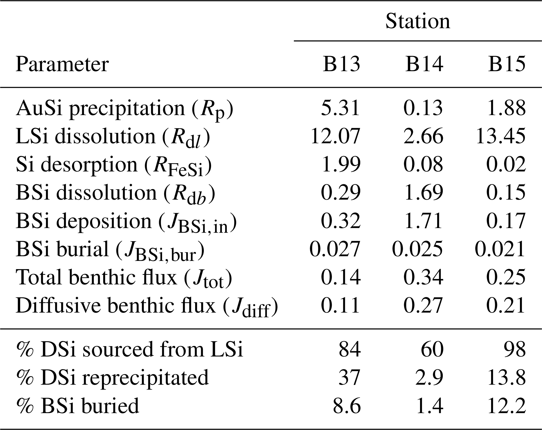
These model observations are consistent with a mass balance calculation using the isotopic compositions of the 0.5 cm pore water sample, as well as the BSi and LSi leachate samples at stations B13 and B14, which indicate a contemporaneous release of both phases. Our model findings therefore support the hypothesis of Ward et al. (2022) that LSi minerals are likely to be dissolving in the upper few centimetres of the Barents Sea seafloor. The depth-integrated reaction rates of the best-fit steady state simulations suggest that between 60 % and 98 % of the DSi released into the sediment pore water from the solid phase is sourced from the dissolution of LSi (Table 2). This range was determined by calculating the depth-integrated rate of LSi dissolution across the model domain and three stations as a proportion of the total integrated rate of DSi input from the three simulated sources (BSi dissolution, LSi dissolution and desorption from metal oxides). The predominance of LSi over BSi dissolution is consistent with the observation that Barents Sea sediments consists of ∼ 96 % terrigenous material (Ward et al., 2022), which is compatible with previous work showing that clay mineral assemblages in the Barents Sea are dominated by terrestrial signals from Svalbard and northern Scandinavia (Vogt and Knies, 2009). The Si isotopic composition of the LSi phase in surface sediments of stations B13, B14 and B15 (−0.89 ± 0.16 ‰; Ward et al., 2022) is also closer to secondary clay minerals (−2.95 ‰ to −0.16 ‰; Opfergelt and Delmelle, 2012, and references therein) than primary silicates of the crust and mantle (∼ 0 ‰ and −0.34 ‰ respectively; Opfergelt and Delmelle, 2012, and references therein). This isotopic composition is not surprising, given the predominance of the clay and silt size fraction in these sediment cores (87 % < 63 µm) (Faust et al., 2020). However, δ30Si measured in the Si-NaOH pool could also represent a combination of reactive primary and secondary silicates, ranging from ∼ 0 ‰ to −2.95 ‰.
While previous mass balance calculations and the model-derived integrated reaction rates presented here agree that both LSi and BSi dissolution contribute to the sediment pore water DSi pool, the magnitudes of the LSi dissolution contribution vary significantly. Ward et al. (2022) suggest that just 14 % and 13 % of the DSi pool in the 0.5 cm pore water interval are sourced from the dissolution of LSi at stations B13 and B14 respectively, while at station B15 it is inferred that the δ30Si can be resolved through BSi dissolution alone. This is in contrast to the 84 %, 60 % and 98 % contributions calculated here (Table 2). There are multiple contributing factors to this discrepancy. Firstly, previous mass balance calculations are based on one depth interval, whereas the estimates presented here are derived from depth-integrated dissolution rates of the entire 50.4 cm model domain. Furthermore, reaction–transport modelling has revealed that this contradiction is likely born of the assumption that the BSi pool at all three stations is sufficient to fuel the pore water DSi stock. Dissolution dynamics were not taken into account in the simple mass balance calculation of Ward et al. (2022); however here we have shown that the composition of Barents Sea surface sediments, which are almost devoid of BSi (0.26 wt %–0.52 wt %, or 92–185 µmol g−1 dry wt), cannot reproduce the rate of pore water DSi build-up with depth from the SWI and can only support an asymptotic DSi concentration of 23 µM at station B15 (dash-dotted blue line, Fig. 3). This observation implies that the additional assumption of Ward et al. (2022) that the 0.5 cm pore water δ30Si value is not impacted by AuSi precipitation could be invalid. If the 0.5 cm pore water interval was directly or indirectly influenced by AuSi precipitation, such an assumption would lead to an underestimation of the LSi contribution as the δ30Si value would be isotopically heavier than if it were derived solely from dissolving solid phases mixing with trapped core top water.
Previously it has been suggested that the quantification of AuSi precipitation rates in marine sediments is not critical in order to fully understand the early diagenetic cycling of Si as reverse weathering typically represents a diagenetic solid-phase conversion from BSi to AuSi, via the dissolved phase (DeMaster, 2019). Model simulations reveal that 37 %, 2.9 % and 13.8 % of the DSi released across the 50 cm model domain at stations B13, B14 and B15 respectively are taken out of solution in the formation of AuSi. This observation is consistent with a similar, previous study of the Peruvian margin upwelling region, which determined that 24 % of DSi released from the dissolution of BSi was reprecipitated as AuSi at a rate of 1.53 mmol Si m−2 d−1 (Ehlert et al., 2016a). AuSi precipitation rates in sediments of the Amazon Delta on the other hand can reach 7.7 mmol Si m−2 d−1 (Michalopoulos and Aller, 2004). Reprecipitation of the DSi pool within the relatively shallow cores studied here will inhibit its exchange with overlying bottom waters. Therefore, in this context, AuSi precipitation can be considered a sink term for the regional Si budget (Ward et al., 2022). In a setting where AuSi precipitation occurs at such a depth where pore water DSi exchange with bottom waters is not possible, this reaction pathway could instead be considered an early diagenetic solid-phase conversion (from BSi and/or LSi to AuSi), as opposed to a true sink term (Frings et al., 2016; DeMaster, 2019).
Table 2Depth-integrated reaction rates of the steady state, best-fit simulations across the upper 50 cm of sediment (Fig. 3), as well as calculated BSi deposition rates and model-derived DSi benthic fluxes. All magnitudes are given in units of mmol Si m−2 d−1.
3.1.2 Evidence for coupling of the benthic Fe and Si cycles in the Barents Sea
Ward et al. (2022) suggest that the benthic Fe and Si cycles are coupled in the Barents Sea, evidenced by a contemporaneous increase in pore water Fe concentrations with an enrichment in the lighter Si isotope of the DSi pool at all three stations. Model simulations support this hypothesis by demonstrating that the Barents Sea DSi pore water profiles can be reconstructed when applying the dissolution of both a BSi and a LSi phase; however under the model scenario where the desorption of FeSi is inhibited (kFeSi=0), the δ30Si pore water profiles are inconsistent with the observational data (solid black lines, Fig. 3). With the dissolution of the LSi phase implemented at both stations B13 and B15, it is possible to resolve the δ30Si pore water profiles in the upper 2.5 and 8.5 cm respectively. However, below these depths the simulated profiles have isotopically heavier compositions than the observational data. Release of an isotopically light phase at specific depth intervals (beginning at 1.5 cm at B13 and 10 cm at B15) results in a simulated δ30Si profile within the range of the observational data (Fig. 3). This isotopic shift to lower pore water δ30Si is interpreted to represent the desorption of Si from solid Fe (oxyhydr)oxide phases, wherein the depth intervals of the same isotopic shifts correspond to the depths at which Fe is released into the pore waters (Faust et al., 2021; Ward et al., 2022). This increase in pore water Fe also occurs at similar depth intervals to decreases in pore water dissolved O2 and concentrations, consistent with a transition from oxic to anoxic conditions (Freitas et al., 2020; Ward et al., 2022).
As discussed above, the Si-HCl reactive Si pool is isotopically light and thought to be associated with metal oxide coatings on BSi (Pickering et al., 2020). The δ30Si composition of the Si-HCl phase is assumed here to represent the composition of the phase desorbing across the Fe redox boundaries. When using a composition of −2.88 ‰ for the FeSi phase, simulation scenarios have identical DSi concentration profiles whether kFeSi is active or set to zero (dashed red and solid black lines, Fig. 3). This similarity is in contrast to the δ30Si pore water profiles, which cannot be reproduced without release of this isotopically light phase at the redox boundaries of all three modelled stations.
This discrepancy between the sediment pore water DSi and δ30Si profiles when the FeSi desorption is active and inactive may explain why the influence of FeSi desorption is so apparent in Barents Sea sediment cores and more ambiguous in similar, previous studies of the Si cycle in lower-latitude marine sediments. The preferential adsorption of 28Si onto Fe (oxyhydr)oxides and the subsequent dissolution or formation of these minerals have been used to interpret both heavy and light δ30Si marine sediment pore water signals in previous work (Ehlert et al., 2016a; Geilert et al., 2020a). In addition, while not inducing a clear signal in the δ30Si, redox cycling of Fe was highlighted as a potential regulating factor in the release of DSi into pore waters of the Greenland margin (Ng et al., 2020). Ng et al. (2020) hypothesised that the reductive dissolution of Fe mineral coatings increased the reactivity of the BSi pool, hence the elevated DSi concentrations found in cores with increased pore water Fe (Ng et al., 2020). In the Barents Sea, FeSi desorption across sedimentary redox boundaries is thought to be so prominent in the δ30Si data because the asymptotic concentration of pore water DSi (∼ 100 µM) is much lower than that in the aforementioned studies (∼ 350–900 µM). The low sediment pore water DSi concentration allows for the direct detection of this process, whereas in previous studies the influence of Fe on the benthic Si cycle is inferred either through elevated DSi and Fe concentrations (Ng et al., 2020) or by depositional context, for example in cores sampled from systems with an abundance of reactive Fe (e.g. hydrothermal vent systems (Fe sulfides) – Geilert et al., 2020a, or the Peruvian oxygen minimum zone – Ehlert et al., 2016a).
At stations B13 and B14, as well as to a lesser extent at B15, there is an increase in the sediment pore water DSi concentration downcore of the middle to the base of the profiles. This feature can be reproduced in the model simulations with the desorption of FeSi from the respective redox boundary depths (Fig. S1); however the required ratio of kFeSi for 28Si and 30Si suggests an isotopic composition of the FeSi phase of just −1.0 ‰ to −1.5 ‰. This isotopic composition is heavier than that measured in the Si-HCl pool (−2.88 ‰), likely reflecting a complexity in the desorption process not captured by the model. Nevertheless, both scenarios support the release of an isotopically light phase at depth, most likely sourced from the Fe redox cycle.
In summary, model simulations somewhat support the hypothesis, based on observational data, that the Barents Sea benthic Si cycle is influenced by the Fe redox system. Model results suggest that the influence of the Fe redox cycle is relatively unimportant for the magnitude of the pore water DSi pool, which appears to be controlled by release from the BSi and LSi phases. However, the coupling of these element cycles is evidenced in the pore water δ30Si data, indicating that the Fe cycle is important for the isotopic budget within the seafloor. We suggest the influence of FeSi desorption is detectable in the Barents Sea pore water δ30Si data, due to the relatively low pore water DSi concentrations and the distinctly isotopically light nature of the FeSi phase. These findings indicate that FeSi desorption should be considered when interpreting downcore δ30Si trends, especially in low-DSi-concentration settings.
3.2 What can transient reaction–transport modelling reveal about non-steady state dynamics in the benthic Si cycle?
Observational pore water DSi concentration data from station B14 suggest that a pulsed increase in the deposition of reactive phytodetritus to the seafloor, derived from phytoplankton blooms, can drive transient peaks in pore water DSi of up to ∼ 300 µM (Ward et al., 2022). This non-steady state dynamic is evidenced in the 3 consecutive years of pore water DSi concentration data collected during the summers of 2017 to 2019, which show that in 2017 and 2019, when the MIZ was above station B14 just 1.5 months prior to sediment coring, a sediment pore water DSi peak is present. This characteristic is in contrast to 2018 when station B14 had been sea-ice-free for 3 months prior to sampling (Downes et al., 2021) and no peak in DSi concentration was observed in the pore water nutrient data (Fig. S6). This observation may indicate that the sediment pore water DSi peaks form under the MIZ, which supports the formation of phytoplankton blooms in late spring/early summer, supplying fresher BSi to the benthos relative to the background BSi pool. Dissolution of this fresher BSi could then fuel subsurface peaks in pore water DSi concentration that dissipate between 1.5 and 3 months after formation, driven by the increased concentration gradient across the SWI that would enhance the rate of molecular diffusion. Additional model simulations were carried out on the baseline, steady state, best-fit model scenario of station B14 to assess this hypothesis.
Results of the transient simulations show that it is possible for the deposition of fresh, bloom-derived BSi to reproduce the observed peaks in pore water DSi concentration in 2017 and 2019 (Fig. 4). Calculated rates of background BSi deposition across the three stations (0.17 to 1.71 mmol Si m−2 d−1, Table 2) are similar to BSi export rates measured in short-term and moored sediment traps in Kongsfjorden, Svalbard at 100 m depth and the eastern Fram Strait at 180–280 m depth (0.2–1.3 mmol Si m−2 d−1) (Lalande et al., 2013, 2016). A simulated 3-week, 10-fold increase in this BSi depositional flux at a much higher reactivity (kdissbloom 20 yr−1) than the background value (kdiss 0.074 yr−1) derived from the 2018 baseline simulation, results in a DSi peak consistent with the magnitude of that in the observational data after 1.5 months (dashed red lines, Fig. 4). This simulated peak in DSi concentration is then able to dissipate by 3 months after bloom initiation. Similarly, with a shorter bloom (1 week), compatible with the typical length of an ice edge bloom in the Barents Sea (Dalpadado et al., 2020) and a 30-fold increase in BSi depositional flux of kdissbloom 15 yr−1, the DSi peak is able to form and dissipate on a time frame similar to that of the former scenario (solid black lines, Fig. 4). The generated peak in DSi concentration must be able to disperse after 3 months if the timing of core sampling relative to MIZ retreat is valid as the explanation for the lack of pore water DSi peak observed in the 2018 data.
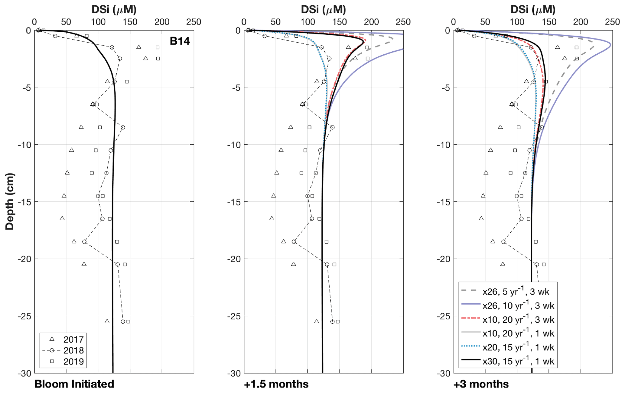
Figure 4Results of the transient simulations under different conditions. Multiplier refers to the increase in the deposition flux (JBSi,in) of the bloom-derived BSi, which was assigned a reactivity (kdissbloom in yr−1) and deposited over either 1 or 3 weeks. Note that the “Bloom Initiated” panel represents the first day of the simulated bloom; therefore all the modelled scenarios overlap and reflect the background steady state simulation. The panels “+1.5 months” and “+3 months” refer to the time elapsed since the bloom was initiated, which are presented to demonstrate how the DSi peak evolves over time. Ward et al. (2022) suggested that DSi peaks could form within 1.5 months and dissipate after 3 months, as evidenced by contrasting sea ice conditions across the three cruises.
The implemented kdissbloom values (5–20 yr−1) are higher than those typically observed in marine sediment cores. kdiss values of 0.98–1.38 yr−1 have been observed at 1 to 20 cm depth in sediment cores collected from the Porcupine Abyssal Plain (mean water depth of 4850 m), considered high for BSi in deep marine sediments (Ragueneau et al., 2001), while values of up to 6.8 yr−1 have been measured in much shallower sediments of Jiaozhou Bay in the Yellow Sea (Wu et al., 2015). kdiss values are highly sensitive to species assemblage and temperature, generally decreasing from the surface ocean towards the seafloor (Natori et al., 2006; Rickert et al., 2002; Rickert, 2000; Roubeix et al., 2008; Kamatani, 1982; Tréguer et al., 1989; Ragueneau et al., 2000). However, kdiss values in fresh diatoms are thought to range from 3 to ∼ 100 yr−1 (Ragueneau et al., 2000; Nelson and Brzezinski, 1997), and previous experiments have measured dissolution rate constants of 27 yr−1 and above (Rickert, 2000; Kamatani and Riley, 1979) at lower temperatures (2–4 ∘C) in seawater, consistent with the values employed in this study. Station B14 is located beneath the polar front, which is a location of intense physical mixing due to the interleaving of multiple water masses (Barton et al., 2018), which has been shown to drive enhanced depositional fluxes of particulate organic carbon relative to that measured both north and south of the frontal zone (Wassmann and Olli, 2004). Furthermore, data collected from sediment traps deployed to the north and north-west of Svalbard have uncovered an approximately 2-fold-higher vertical carbon export flux from diatomaceous aggregates formed in seasonally sea-ice-covered regions, compared with aggregates from P. pouchetii blooms (Fadeev et al., 2021; Dybwad et al., 2021). Therefore, it is considered here that given the shallow depth of the Barents Sea seafloor and the location of station B14 beneath the polar front, fresh and reactive BSi formed in MIZ blooms could be efficiently ferried to the seafloor.
The kdissbloom of the bloom-derived BSi is much higher than that required to reproduce the solid-phase BSi content profiles of the background system (kdiss) (Fig. 3). At stations B13, B14 and B15, the implemented kdiss values in the steady state simulations were 0.0055, 0.074 and 0.0105 yr−1 respectively (Table S2, Fig. 2), which are not dissimilar to those estimated for deep-sea sediments from DSi pore water profile-fitting procedures and flow-through reactor experiments (0.006–0.44 yr−1) (McManus et al., 1995; Rabouille et al., 1997; Ragueneau et al., 2001; Rickert, 2000). The inverse of the dissolution rate constant provides an estimate of the residence time or mean lifetime of the given pool of BSi (McManus et al., 1995), which suggests that the less reactive pool of BSi has a mean lifetime of 182, 13.5 and 95 years at stations B13, B14 and B15 respectively. These mean lifetimes are too long to influence the Si cycle on a seasonal scale, which must be < 1 yr−1 to do so, as is the case for organic matter (Burdige, 2006). The model-derived estimates of kdissbloom on the other hand would suggest a mean lifetime of approximately 20 d for the fresh BSi.
Therefore, this work suggests that there are at least two types of BSi in Barents Sea sediments, one less reactive pool that dissolves at a slower rate and one fresher, bloom-derived pool that is able to perturb the sediment pore water DSi stock on a seasonal timescale. This conclusion is compatible with findings from a study of the equatorial Pacific region (McManus et al., 1995) and observations from the Arabian Sea, indicating that the bulk sediment BSi content should not be treated as a single pool of uniform reactivity but should instead be separated into reactive and unreactive fractions (Rickert, 2000; Schink et al., 1975). Consistent with these conclusions, previous experiments have demonstrated that dissolution patterns of some diatom frustules can be best described by two kdiss values, an order of magnitude apart (Boutorh et al., 2016; Moriceau et al., 2009). These results indicate the presence of two phases of BSi within diatom frustules, denoting a potential physiological basis for the differentiation in reactivity of seafloor BSi.
3.3 What is the simulated benthic DSi flux, and how important is the contribution of bloom-derived BSi dissolution to the annual flux?
The simulated Jdiff magnitudes (0.11–0.27 mmol Si m−2 d−1) that contribute to Jtot (Table 2) are within error of previously calculated Jdiff values (0.10–0.37 mmol Si m−2 d−1) for these Barents Sea sediment cores (Ward et al., 2022). Thus, our model-derived benthic DSi fluxes are well within the range of a compilation of pan-Arctic shelf benthic DSi fluxes (−0.03 to +6.2 mmol Si m−2 d−1) (Bourgeois et al., 2017). Based on previous calculations and the simulation results presented here, we estimate that the mean DSi Jdiff benthic flux magnitude for the Barents Sea is +0.23 (±0.11 1σ) mmol Si m−2 d−1, ranging from +0.08 to +0.54 mmol Si m−2 d−1.
Jtot at all stations is dominated by the molecular diffusive component (Jdiff) (76 %–85 %), in agreement with simulated estimates of phosphate fluxes at the same stations (Freitas et al., 2020) (Fig. 5). Jtot at station B13 has the highest contribution from bioturbation (6 %), consistent with the highest experimentally determined bioturbation diffusion coefficient of the Barents Sea stations (Solan et al., 2020). The advective component of Jtot is negligible at all stations, while the bioirrigation element represents the greatest source of uncertainty in the simulated flux magnitudes as this parameter was not constrained in parallel to this work; thus a global value was assumed (Thullner et al., 2009). At station B15, the model-derived Jtot (+0.25 mmol Si m−2 d−1) is greater than JBSi,in (0.17 mmol Si m−2 d−1) (Table 2). This observation points to the release of an additional source of DSi to the dissolving BSi, which is compatible with the hypothesis that LSi is being released into the pore water dissolved phase.
DSi benthic flux magnitudes were also calculated for the transient simulations carried out on station B14 to quantify the influence of fresh bloom-derived BSi. Dissolution of the fresher BSi has an immediate and significant effect on the benthic flux, doubling the steady state background value of +0.34 to +0.66 mmol Si m−2 d−1 within 1 week, which peaks 2 weeks after bloom material deposition at +1.84 mmol Si m−2 d−1, representing a 5-fold increase (an additional +1.5 mmol Si m−2 d−1) in the background steady state benthic flux magnitude. The prominent DSi peak then dissipates and becomes largely undetectable after 3 months (Fig. 4). The average DSi benthic flux at the SWI over the 12-week period is +1.07 mmol Si m−2 d−1, indicating that the bloom-derived BSi releases an additional +0.73 mmol Si m−2 d−1 to the overlying bottom water. The steady state and transient model simulations therefore suggest that the background benthic flux of Si from the benthos is +124 mmol Si m−2 yr−1 at station B14, while the additional contribution over the 12-week period sourced from fresh BSi dissolution is +61.3 mmol Si m−2 (based on a rate of +0.73 mmol Si m−2 d−1). This estimate suggests that a minimum of 33 % of the total annual benthic flux of DSi discharging from the seafloor at station B14 is sourced from the deposition of fresh BSi during the 1-week MIZ bloom.
The contribution of bloom-derived BSi dissolution to the annual benthic DSi flux magnitude reported here (an additional +0.73 mmol Si m−2 d−1 over the 3 months) for station B14 is greater than that in Ward et al. (2022) (an additional +0.23 mmol Si m−2 d−1 over the same time interval), although the proportion is consistent across the two estimates (approximately one-third of the total annual benthic DSi flux). In part, this is due to the simulated fluxes incorporating the contribution from bioirrigation and bioturbation (Jtot). When using only the simulated Jdiff component, an additional +0.46 mmol Si m−2 d−1 is estimated to be sourced from the bloom-derived BSi, which is more consistent with the observational data calculations. However, this disparity is also due to the nature of the simulated flux calculation. The model-derived benthic flux magnitudes are calculated at the SWI, whereas previous Jdiff estimates are based on observational data of a much lower resolution, with the concentration gradient determined based on the DSi concentration in the core top water and in the sediment pore water at 0.5 cm depth. Furthermore, the simulated benthic flux estimates are based on a mean value derived from a weekly temporal resolution, which is not accessible in the observational data. However, both estimates can be used to draw a range of possible contributions from the bloom-derived BSi, and although there is a disparity in the benthic flux magnitude, both methodologies suggest that at least one-third of the annual DSi benthic flux at station B14 is sourced from the dissolution of BSi deposited after a short MIZ bloom.
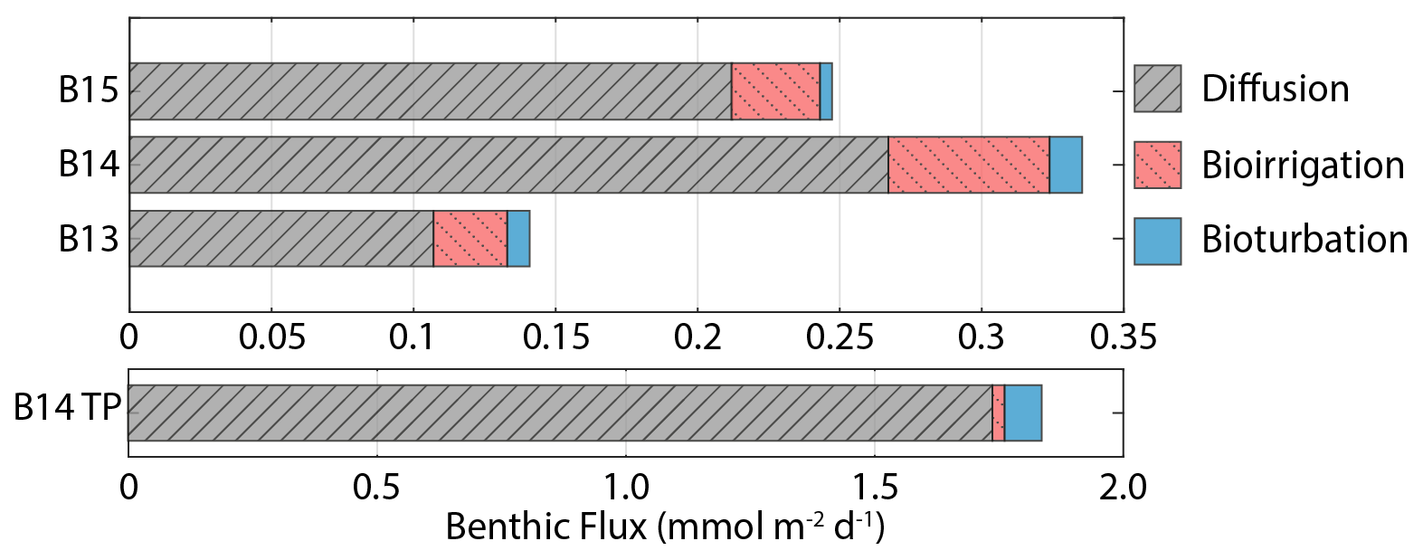
Figure 5Benthic DSi flux magnitudes at the SWI calculated from steady state simulations, including contributions from molecular diffusion, bioirrigation and bioturbation. B14 TP refers to the B14 DSi flux magnitude at the peak of the transient simulations (×30 BSi depositional flux, 15 yr−1 kdissbloom, 1-week bloom duration).
3.4 How much BSi is buried in the long term in the Barents Sea?
Traditionally, burial efficiencies of BSi were not included within Si budgets of the Arctic Ocean due in part to a low mean BSi content (< 5 wt %), as well as to a low estimated sedimentation rate (a few mm kyr−1) (Brzezinski et al., 2021; März et al., 2015). However, more recently Arctic Ocean seafloor BSi burial efficiencies are being re-evaluated due to revised models of sediment accumulation rates (Brzezinski et al., 2021). Asymptotic BSi content profiles approach 0.2 wt % at 14.5 cm below the SWI and remain constant with depth at all three Barents Sea stations (Figs. 3, S2), suggesting that some BSi is buried and able to accumulate in the seabed. Assuming a sedimentation rate of 0.05–0.06 cm yr−1 (Zaborska et al., 2008), BSi particulates deposited at the SWI would approach 14.5 cm depth within approximately 240–300 years due to sediment accumulation, where BSi dissolution appears to cease. This timescale is of a similar magnitude to the calculated mean lifetime based on kdiss from the model simulations at station B13 (182 years), indicating that some BSi from this pool could accumulate at depth. However, the steady state BSi pools at stations B14 and B15 have mean lifetimes of just 95 and 13.5 years respectively, theoretically precluding burial of this pool below 14.5 cm depth. The observation that BSi is present at ∼ 40 cm depth at all three stations with a concentration of ∼ 0.2 wt % indicates that there may be three fractions of BSi constituting the bulk BSi phase: fresh bloom-derived BSi represented by kdissbloom, the less reactive background BSi (kdiss) and a non-reactive pool that contributes to the 0.2 wt % BSi at depth alongside any surviving component from the background pool. A mean BSi burial rate of 0.024 mmol Si m−2 d−1 is estimated here for the Barents Sea (Eq. 7, Table 2), corresponding to 0.012 Tmol Si yr−1 for the whole shelf, assuming an area of 1.4×10⁶ km2.
Global seafloor BSi burial efficiencies (calculated as the BSi burial flux divided by the deposition rate) range from 1 %–97 % (Westacott et al., 2021; Frings, 2017; Ragueneau et al., 2001, 2009; DeMaster, 2001; DeMaster et al., 1996; Liu et al., 2005), averaging ∼ 11 % (Tréguer et al., 2021; Frings, 2017). Typically, BSi burial efficiencies are much higher in coastal and shelf settings and underneath polar fronts, due in part to higher rates of sedimentation (DeMaster, 2001). Indeed, studies of the Southern Ocean (Indian sector and the Ross Sea) and the Peruvian margin uncovered a 4- to 30-fold increase in BSi burial efficiency at the continental shelf stations (22 %–58 %), relative to the open-ocean counterparts (2 %–17 %) (Dale et al., 2021; DeMaster, 2001; Ragueneau et al., 2001). BSi burial efficiencies estimated here for three Barents Sea stations (1.4 %–12 %, Table 2) are within the range of published values and similar to the global mean at stations B13 and B15 but low relative to other continental shelves. Our estimated BSi burial efficiencies are based on the same sedimentation rates employed in the model (Table S2), which are similar to the Barents Sea mean of 0.07 cm yr−1 (Zaborska et al., 2008). However, Barents Sea sedimentation rates of up to 0.21 cm yr−1 have been estimated since the last glacial period (Faust et al., 2021), which would significantly increase the estimated BSi burial efficiencies (5 %–33 %) (Eq. 7).
While the BSi burial efficiency calculated at station B14 is also within previously published values, it is much lower than the Barents Sea stations to the north and south. Solid-phase BSi contents in the surface intervals were determined from samples collected during the third cruise in summer 2019. As discussed, the pore water DSi profiles at B14 from this cruise are thought to be influenced by the dissolution of bloom-derived BSi, which would account for the elevated BSi content in the surface sediment relative to that at stations B13 and B15. The higher BSi content has likely resulted in an elevated estimation of JBSi,in and thus a reduced burial efficiency, which would also explain why the model-derived estimate of the contribution of LSi dissolution to the DSi released from the solid phase is lower at station B14 (60 %), due to an elevated Rdb, which is enhanced by the deposition of fresher BSi. In addition, this would also explain why the estimated mean lifetime of the BSi from the steady state simulations at station B14 is much shorter than for the other two sites (13.5 years vs. 95–182 years). If the measured surface BSi content at station B14 is indeed influenced by residual bloom-derived BSi, this would result in an overestimate of the background BSi reactivity in the model.
Relatively low burial efficiencies of BSi in sediments underneath oxygen-depleted bottom waters (7 %–12 %), similar in magnitude to those calculated here for the Barents Sea, have previously been attributed to low rates of bioturbation, resulting in less efficient export of BSi towards more saturated pore waters (Dale et al., 2021). Bioturbation coefficients were determined experimentally for the Barents Sea stations (2–6 cm−2 yr−1) (Table S2) and are much lower than might be expected, based on an empirical global relationship with water depth (∼ 24 cm−2 yr−1) (Middelburg et al., 1997). Furthermore, the impacts of the low rates of macrofaunal mixing on BSi burial efficiency are likely exacerbated by slow rates of sediment accumulation in the Barents Sea. High rates of BSi burial in the Bohai Sea (60 %) and Yellow Sea (42 %) are thought to be driven by high sediment accumulation rates (Liu et al., 2002), which as with bioturbation is much lower in the Barents Sea than might be expected based on an empirical global relationship with water depth (0.55 cm yr−1) (Middelburg et al., 1997). The combination of low rates of macrofaunal mixing and sediment accumulation may therefore be the cause of the lower BSi burial efficiencies observed here relative to other continental shelves.
3.5 What are the implications of this work for the Arctic Ocean Si budget?
Brzezinski et al. (2021) uncovered an imbalance in the Arctic Ocean Si budget after carrying out an assessment using Si isotopes. The δ30Si values measured in the main Arctic Ocean water mass inflow and outflows are similar (∼ +1.70 ‰; Giesbrecht, 2019; Liguori et al., 2020; Brzezinski et al., 2021), suggesting that the cycling of Si within the Arctic Ocean has little net effect on δ30Si. Brzezinski et al. (2021) conclude that given the relatively isotopically light input from fluvial sources (+1.30 ± 0.3 ‰; Sun et al., 2018), as well as that emerging from seafloor sediments (+1.16 ± 0.11 ‰; Ward et al., 2022), balance must be maintained through the burial of isotopically light Si by BSi. However, a mass balance showed that the isotopically light inputs to the system are only partially offset by the burial of BSi (0.16–0.30 Tmol Si yr−1), assumed to have a δ30Si of +1.16 ± 0.10 ‰ (Brzezinski et al., 2021). There must therefore be an additional sink of isotopically light Si if the Arctic Ocean Si isotope budget is to maintain balance (Fig. 6). The absence of direct isotopic observations from some of the major gateways, including the Barents Sea shelf over which most of the DSi sourced from the Atlantic Ocean flows (Torres-Valdés et al., 2013), as well as a lack of data for the isotopic composition of BSi in Arctic Ocean sediments, must be addressed to confirm the mechanisms proposed by Brzezinski et al. (2021). Si isotopes measured in the weak alkaline leachate (0.1 M Na2CO3, δ30SiAlk) extracted from surface sediment sequential digestion experiments and measurements of δ30Si in core top waters (Ward et al., 2022), coupled with reaction–transport modelling (this study) for stations B13, B14 and B15, contribute to the Arctic Ocean Si isotope dataset and help to fill these knowledge gaps.
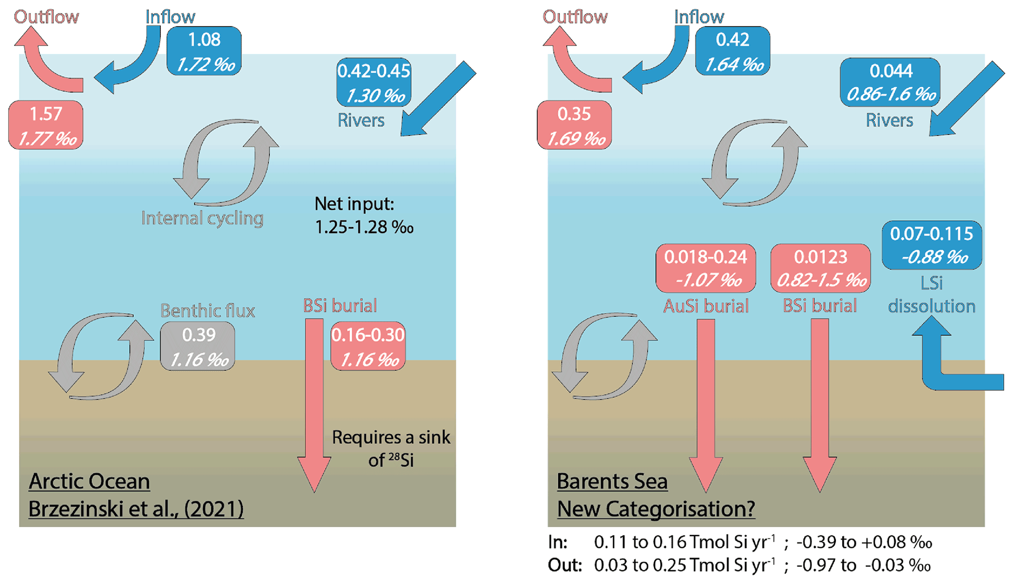
Figure 6The Arctic Ocean Si budget (Brzezinski et al., 2021) (left) and a proposed Si budget for the Barents Sea (right), including a benthic flux recategorisation (i.e. contributions from BSi and LSi) and AuSi burial. Boxes include flux magnitudes given in Tmol Si yr−1 (top values) and the flux δ30Si in per mille (‰; italicised bottom values). “In” and “Out” refer to the Si fluxes, discounting the water mass inflow and outflow (i.e. in (blue) includes rivers + LSi; out (red) includes AuSi + BSi). Grey boxes and arrows represent internal cycling. See Supplement Sect. 3 for further information on how the Barents Sea Si budget was calculated.
δ30SiAlk in the Barents Sea ranges from +0.82 ± 0.16 ‰ at station B15 to +1.50 ± 0.19 ‰ at B14 (Ward et al., 2022). The Na2CO3 leachate activates an operationally defined reactive pool of Si, thought to be associated with authigenically altered and unaltered BSi (Pickering et al., 2020). Molar ratios of the Na2CO3 support this concept, which fall within the range of that expected of BSi (Ward et al., 2022). δ30Si values measured in the core top waters at the Atlantic Water station (B13, +1.64 ± 0.19 ‰) and Arctic Water station (B15, +1.69 ± 0.18 ‰) are similar to the composition of the main Arctic Ocean inflow and outflow water masses (∼ 1.7 ‰) (Giesbrecht, 2019; Brzezinski et al., 2021; Liguori et al., 2020) and heavier than that measured in the BSi deposited at the seafloor. Therefore, assuming the composition of the BSi below the BSi dissolution zone within the seafloor is similar to that at the SWI, Barents Sea sediments represent a sink of 28Si, relative to the composition of the inflow waters. However, δ30SiAlk at stations B13 and B14 is still isotopically heavier than the Arctic Ocean riverine input (+1.30 ± 0.3 ‰), as well as the assumed composition of the BSi buried across the Arctic seabed (+1.16 ± 0.10 ‰) in the Si budget (Brzezinski et al., 2021) (Fig. 6). Through reaction–transport modelling we have estimated that between 2 % and 40 % of the sediment pore water DSi pool is sourced from the dissolution of BSi. Moreover, 2.9 %–37 % of the total amount of DSi released is reprecipitated as AuSi (Table 2). AuSi preferentially takes up the lighter isotope in the Barents Sea with a 30ϵ of −2.0 ‰ to −2.3 ‰ (Table S2), thereby enhancing the preservation of BSi and further enriching the solid phase in the lighter isotope. Clays formed during weathering have a δ30Si composition ranging from −2.95 ‰ to −0.16 ‰ (Opfergelt and Delmelle, 2012). The burial of AuSi alongside BSi could therefore account for some of the isotopic imbalance.
Our reaction–transport model study has also highlighted the important contribution of LSi dissolution to the sediment pore water DSi pool (60 %–98 %). If our findings on the dissolution of LSi are consistent across other Arctic shelves, a portion of the benthic DSi flux cannot be defined as internal cycling of Si and should be recategorised as an additional input to that from the major ocean gateways and discharge from rivers. It is currently estimated that the benthic flux of DSi across the whole Arctic Ocean seafloor is ∼ 0.39 Tmol Si yr−1 (März et al., 2015); therefore between 0.23 and 0.38 Tmol Si yr−1 may represent an input of Si rather than a recycling term. This recategorisation could account for the additional Si inputs required to close the Si budget, as currently 32 %–47 % (or 0.21–0.38 Tmol Si yr−1) of the estimated net Si output is unaccounted for (Brzezinski et al., 2021). The addition of AuSi as an output to resolve the isotopic imbalance would offset to some extent the release of DSi from LSi, while the LSi input compounds the isotopic imbalance identified by Brzezinski et al. (2021). However, here we show that through AuSi precipitation acting as an additional sink for 28Si, both mass and isotopic balance can be attained in our proposed Si budget for the Barents Sea (Fig. 6, Supplement Sect. S3). Future work should look to assess whether similar relationships exist between the dissolution of LSi and precipitation of AuSi on other Arctic Ocean shelves if we are to use these mechanisms to balance the pan-Arctic Si budget. Additional work could include empirical assessments, such as through batch or flow-through reactor experiments, to study dissolution (both BSi and LSi) and precipitation (AuSi) kinetics in Arctic Ocean sediments and to further examine and better constrain the relationship between benthic Si and Fe redox cycles.
In this study we quantify and disentangle the processes involved in the early diagenetic cycling of Si in the Arctic Barents Sea seafloor by reproducing Si isotopic and DSi concentration data from the solid and dissolved phase in a reaction–transport model (Figs. 2 and 3). Baseline simulations are able to reproduce the observational data well; however we have also shown that the benthic Si cycle is responsive on the order of days to the delivery of fresh BSi. Therefore, while the transient disturbances appear to be short-lived, future work should look to incorporate these processes into the baseline simulations.
Baseline model simulations also reveal that a significant proportion of the Si released from the solid phase within Barents Sea surface sediments is sourced from the dissolution of LSi (60 %–98 %) on account of the low BSi contents (0.26 wt %–0.52 wt %). Furthermore, we demonstrate that without the influence of the Fe redox cycle, which results in the release of Si adsorbed onto solid Fe (oxyhydr)oxides under anoxic conditions, the observed isotopic composition of the pore water DSi pool cannot be reconciled. Both the LSi and FeSi sources are depleted in the heavier isotope (−0.89 ‰ and −2.88 ‰ respectively), as demonstrated in a sequential digestion experiment (Ward et al., 2022), consistent with the observation that sediments of the Barents Sea represent a source of light DSi to the overlying bottom waters (Brzezinski et al., 2021). Of the DSi sourced from BSi, LSi and FeSi, we show that between 2.9 % and 37 % is reprecipitated as AuSi. Coupled with the observation that a significant proportion of the sediment pore water DSi pool is sourced from the dissolution of LSi, this hypothesis is significant for the regional Si budget. The dissolution of LSi represents a source of “new” Si to the ocean DSi pool, and the precipitation of AuSi inhibits exchange of pore water DSi with overlying bottom waters and therefore represents a sink term. These observations could require a recategorisation of a portion of the benthic flux in the Arctic Ocean Si budget, which is currently defined as a recycling term, as well as the inclusion of an additional Si sink. If LSi dissolution and AuSi precipitation are not exclusive to the Barents Sea shelf, the additional input and isotopically light output could account for both the isotopic imbalance and the remaining proportion of net Si outflow that is currently unaccounted for (Brzezinski et al., 2021).
Model simulations also highlight a dichotomy in the cycling of Si in the Barents Sea seafloor, which is hypothesised to occur on at least two timescales. Observational data at stations B13 and B15 can be reproduced by assuming a steady state dynamic, thus representing a background system, which is controlled by the release of Si into the DSi pool from LSi and the reprecipitation of DSi as AuSi. However, sampling across 3 years at station B14 has uncovered Si cycling on a much shorter timescale, controlled by the deposition of fresh phytodetritus. In this transient dynamic, the release of DSi is controlled by the dissolution of more reactive BSi. The processes occurring on the former steady state time frame will likely remain largely unaltered with further Atlantification of the Barents Sea due to the mineralogical control on DSi release, whereas the latter transient system is reliant upon the seasonal delivery of fresh BSi, which is subject to change as the community compositions of the MIZ and spring phytoplankton blooms shift to favour temperate Atlantic flagellate species (Neukermans et al., 2018; Orkney et al., 2020) or diatoms with lower silica content than polar species (Lomas et al., 2019). Furthermore, we have shown that the benthic DSi flux magnitude can increase 5-fold after a simulated 1-week bloom, which is calculated here to contribute a minimum of one-third of the total annual flux of DSi from the seafloor at station B14. Any perturbation in the delivery of bloom-derived, relatively reactive BSi to the seafloor could therefore be detrimental to the total annual supply of DSi from Barents Sea sediments.
Research data associated with this article can be accessed at https://doi.org/10.5285/8933AF23-E051-4166-B63E-2155330A21D8 (Ward et al., 2021b). Reaction–transport model code (Si BRNS) can be accessed at https://doi.org/10.5281/zenodo.6023767 (Ward et al., 2021a).
The supplement related to this article is available online at: https://doi.org/10.5194/bg-19-3445-2022-supplement.
JCF, FSF, SFH and ACT helped in the sampling and processing of onboard samples. SFH and JPJW measured Si concentrations; JPJW carried out Si isotopic analysis. JPJW and KRH designed the sediment digestion experiments, carried out by JPJW. JCF, CM and ACT measured pore water major and trace element concentrations, and RLA conducted surface sediment pigment analysis. SA, FSF and JPJW developed the steady state and transient model code; JPJW performed the simulations. All authors contributed to data interpretation. JPJW prepared the manuscript with contributions from all authors.
The contact author has declared that none of the authors has any competing interests.
Publisher’s note: Copernicus Publications remains neutral with regard to jurisdictional claims in published maps and institutional affiliations.
This work formed part of the Changing Arctic Ocean Seafloor project (ChAOS) of the Changing Arctic Ocean programme, funded by the UKRI Natural Environment Research Council (NERC). We would like to express our gratitude to the captain and crew of RRS James Clark Ross for their support on cruises JR16006, JR17007 and JR18006. Additional logistical support was provided by National Marine Facilities and the British Antarctic Survey. Further thanks go to colleagues for their support and advice, including Christopher Coath, Lucie Cassarino, Jade Hatton, Stephanie Bates, Rachael Ward, Adam McAleer, Rebecca Pickering, Hong Chin Ng, Matteo Puglini, Joshua Lucas, Alex Stewart and Jason Sharkey. Finally, we would like to thank the editor and reviewers for their constructive comments and feedback to help improve this article.
This research has been supported by the Natural Environment Research Council (grant nos. NE/P005942/1, NE/P006108/1 and NE/P006493/1).
This paper was edited by Jack Middelburg and reviewed by two anonymous referees.
Aguilera, D. R., Jourabchi, P., Spiteri, C., and Regnier, P.: A knowledge-based reactive transport approach for the simulation of biogeochemical dynamics in Earth systems, Geochem. Geophy. Geosy., 6, https://doi.org/10.1029/2004GC000899, 2005. a
Aller, R. C.: 8.11 – Sedimentary Diagenesis, Depositional Environments, and Benthic Fluxes, Treatise on Geochemistry, 2nd Edn., 8, 293–334, https://doi.org/10.1016/B978-0-08-095975-7.00611-2, 2014. a, b
Årthun, M., Eldevik, T., Smedsrud, L. H., Skagseth, and Ingvaldsen, R. B.: Quantifying the influence of atlantic heat on barents sea ice variability and retreat, J. Clim., 25, 4736–4743, https://doi.org/10.1175/JCLI-D-11-00466.1, 2012. a, b, c
Backman, J., Jakobsson, M., Løvlie, R., Polyak, L., and Febo, L. A.: Is the central Arctic Ocean a sediment starved basin?, Quaternary Sci. Rev., 23, 1435–1454, https://doi.org/10.1016/j.quascirev.2003.12.005, 2004. a
Barton, B. I., Lenn, Y. D., and Lique, C.: Observed atlantification of the Barents Sea causes the Polar Front to limit the expansion of winter sea ice, J. Phys. Oceanogr., 48, 1849–1866, https://doi.org/10.1175/JPO-D-18-0003.1, 2018. a, b
Berner, R.: Early diagenesis: a theoretical approach, Princeton University Press, Princeton, NJ, ISBN 9780691082608, 1980. a
Boudreau, B. P.: Diagenetic models and their implementation: modelling transport and reactions in aquatic sediments, Springer, New York, 1st Edn., ISBN 3540611258, 1997. a, b
Bourgeois, S., Archambault, P., and Witte, U.: Organic matter remineralization in marine sediments: A Pan-Arctic synthesis, Global Biogeochem. Cy., 31, 190–213, https://doi.org/10.1002/2016GB005378, 2017. a
Boutorh, J., Moriceau, B., Gallinari, M., Ragueneau, O., and Bucciarelli, E.: Effect of trace metal-limited growth on the postmortem dissolution of the marine diatom Pseudo-nitzschia delicatissima, Global Biogeochem. Cy., 30, 57–69, https://doi.org/10.1002/2015GB005088, 2016. a
Brzezinski, M. A., Closset, I., Jones, J. L., de Souza, G. F., and Maden, C.: New Constraints on the Physical and Biological Controls on the Silicon Isotopic Composition of the Arctic Ocean, Front. Mar. Sci., 8, 699762, https://doi.org/10.3389/fmars.2021.699762, 2021. a, b, c, d, e, f, g, h, i, j, k, l, m, n, o, p, q, r
Burdige, D.: Geochemistry of Marine Sediments, Princeton University Press, Princeton, NJ, ISBN 9780691095066, 2006. a, b
Cassarino, L., Hendry, K. R., Henley, S. F., MacDonald, E., Arndt, S., Freitas, F. S., Pike, J., and Firing, Y. L.: Sedimentary Nutrient Supply in Productive Hot Spots off the West Antarctic Peninsula Revealed by Silicon Isotopes, Global Biogeochem. Cy., 34, https://doi.org/10.1029/2019GB006486, 2020. a, b, c
Cochrane, S. K., Denisenko, S. G., Renaud, P. E., Emblow, C. S., Ambrose, W. G., Ellingsen, I. H., and Skardhamar, J.: Benthic macrofauna and productivity regimes in the Barents Sea – Ecological implications in a changing Arctic, J. Sea Res., 61, 222–233, https://doi.org/10.1016/j.seares.2009.01.003, 2009. a
Dale, A. W., Paul, K. M., Clemens, D., Scholz, F., Schroller-Lomnitz, U., Wallmann, K., Geilert, S., Hensen, C., Plass, A., Liebetrau, V., Grasse, P., and Sommer, S.: Recycling and Burial of Biogenic Silica in an Open Margin Oxygen Minimum Zone, Global Biogeochem. Cy., 35, https://doi.org/10.1029/2020GB006583, 2021. a, b
Dalpadado, P., Arrigo, K. R., van Dijken, G. L., Skjoldal, H. R., Bagøien, E., Dolgov, A. V., Prokopchuk, I. P., and Sperfeld, E.: Climate effects on temporal and spatial dynamics of phytoplankton and zooplankton in the Barents Sea, Prog. Oceanogr., 185, 102320, https://doi.org/10.1016/j.pocean.2020.102320, 2020. a, b
De La Rocha, C. L., Brzezinski, M. A., and DeNiro, M. J.: Fractionation of silicon isotopes by marine diatoms during biogenic silica formation, Geochim. Cosmochim. Ac., 61, 5051–5056, https://doi.org/10.1016/S0016-7037(97)00300-1, 1997. a
Degerlund, M. and Eilertsen, H. C.: Main Species Characteristics of Phytoplankton Spring Blooms in NE Atlantic and Arctic Waters (68–80∘ N), Estuaries Coast, 33, 242–269, https://doi.org/10.1007/s12237-009-9167-7, 2010. a
Delstanche, S., Opfergelt, S., Cardinal, D., Elsass, F., André, L., and Delvaux, B.: Silicon isotopic fractionation during adsorption of aqueous monosilicic acid onto iron oxide, Geochim. Cosmochim. Ac., 73, 923–924, https://doi.org/10.1016/j.gca.2008.11.014, 2009. a, b
Demarest, M. S., Brzezinski, M. A., and Beucher, C. P.: Fractionation of silicon isotopes during biogenic silica dissolution, Geochim. Cosmochim. Ac., 73, 5572–5583, https://doi.org/10.1016/j.gca.2009.06.019, 2009. a
DeMaster, D.: Marine Silica Cycle, in: Encyclopedia of Ocean Sciences, Academic Press, 1659–1667, https://doi.org/10.1006/rwos.2001.0278, 2001. a, b, c
DeMaster, D. J.: The global marine silica budget: Sources and sinks, in: Encyclopedia of Ocean Sciences, Elsevier Ltd., 473–483, https://doi.org/10.1016/B978-0-12-409548-9.10799-7, 2019. a, b
DeMaster, D. J., Ragueneau, O., and Nittrouer, C. A.: Preservation efficiencies and accumulation rates for biogenic silica and organic C, N, and P in high-latitude sediments: The Ross Sea, J. Geophys. Res.-Ocean., 101, 18501–18518, https://doi.org/10.1029/96JC01634, 1996. a
Dixit, S., Van Cappellen, P., and Van Bennekom, A. J.: Processes controlling solubility of biogenic silica and pore water build-up of silicic acid in marine sediments, Mar. Chem., 73, 333–352, https://doi.org/10.1016/S0304-4203(00)00118-3, 2001. a
Downes, P. P., Goult, S. J., Woodward, E. M. S., Widdicombe, C. E., Tait, K., and Dixon, J. L.: Phosphorus dynamics in the Barents Sea, Limnol. Oceanogr., 66, S326–S342, https://doi.org/10.1002/lno.11602, 2021. a
Druzhkova, E., Oleinik, A., and Makarevich, P.: Live autochthonous benthic diatoms on the lower depths of Arctic continental shelf, Preliminary results, Oceanologia, 60, 97–100, https://doi.org/10.1016/j.oceano.2017.07.001, 2018. a
Dybwad, C., Assmy, P., Olsen, L. M., Peeken, I., Nikolopoulos, A., Krumpen, T., Randelhoff, A., Tatarek, A., Wiktor, J. M., and Reigstad, M.: Carbon Export in the Seasonal Sea Ice Zone North of Svalbard From Winter to Late Summer, Front. Mar. Sci., 7, 525800. https://doi.org/10.3389/fmars.2020.525800, 2021. a, b
Egan, K. E., Rickaby, R. E., Leng, M. J., Hendry, K. R., Hermoso, M., Sloane, H. J., Bostock, H., and Halliday, A. N.: Diatom silicon isotopes as a proxy for silicic acid utilisation: A Southern Ocean core top calibration, Geochim. Cosmochim. Ac., 96, 174–192, https://doi.org/10.1016/j.gca.2012.08.002, 2012. a
Ehlert, C., Doering, K., Wallmann, K., Scholz, F., Sommer, S., Grasse, P., Geilert, S., and Frank, M.: Stable silicon isotope signatures of marine pore waters – Biogenic opal dissolution versus authigenic clay mineral formation, Geochim. Cosmochim. Ac., 191, 102–117, https://doi.org/10.1016/j.gca.2016.07.022, 2016a. a, b, c, d, e, f, g, h, i, j, k, l
Ehlert, C., Reckhardt, A., Greskowiak, J., Liguori, B. T., Böning, P., Paffrath, R., Brumsack, H. J., and Pahnke, K.: Transformation of silicon in a sandy beach ecosystem: Insights from stable silicon isotopes from fresh and saline groundwaters, Chem. Geol., 440, 207–218, https://doi.org/10.1016/j.chemgeo.2016.07.015, 2016b. a, b
Fabre, S., Jeandel, C., Zambardi, T., Roustan, M., and Almar, R.: An Overlooked Silica Source of the Modern Oceans: Are Sandy Beaches the Key?, Front. Earth Sci., 7, 231, https://doi.org/10.3389/feart.2019.00231, 2019. a, b
Fadeev, E., Rogge, A., Ramondenc, S., Nöthig, E.-M., Wekerle, C., Bienhold, C., Salter, I., Waite, A. M., Hehemann, L., Boetius, A., and Iversen, M. H.: Sea ice presence is linked to higher carbon export and vertical microbial connectivity in the Eurasian Arctic Ocean, Commun. Biol., 4, 1255, https://doi.org/10.1038/s42003-021-02776-w, 2021. a, b, c
Fanning, K. A. and Schink, D. R.: Interaction of Marine Sediments with Dissolved Silica, Limnol. Oceanogr., 14, 59–68, https://doi.org/10.4319/lo.1969.14.1.0059, 1969. a
Faust, J. C., Stevenson, M., Abbott, G., and Knies, J.: Does Arctic warming reduce preservation of organic matter in Barents Sea sediments?, Philos. T. R. Soc. A, 378, 2181, https://doi.org/10.1098/rsta.2019.0364, 2020. a, b
Faust, J. C., Tessin, A., Fisher, B. J., Zindorf, M., Papadaki, S., Hendry, K. R., Doyle, K. A., and März, C.: Millennial scale persistence of organic carbon bound to iron in Arctic marine sediments, Nat. Commun., 12, 2181, https://doi.org/10.1038/s41467-020-20550-0, 2021. a, b, c
Freitas, F. S., Hendry, K. R., Henley, S. F., Faust, J. C., Tessin, A. C., Stevenson, M. A., Abbott, G. D., März, C., and Arndt, S.: Benthic-pelagic coupling in the Barents Sea: an integrated data-model framework, Philos. T. R. Soc. A, 378, 2181, https://doi.org/10.1098/rsta.2019.0359, 2020. a, b, c, d
Freitas, F. S., Pika, P. A., Kasten, S., Jorgensen, B. B., Rassmann, J., Rabouille, C., Thomas, S., Sass, H., Pancost, R. D., and Arndt, S.: New insights into large-scale trends of apparent organic matter reactivity in marine sediments and patterns of benthic carbon transformation, Biogeosciences, 18, 4651–4679, https://doi.org/10.5194/bg-18-4651-2021, 2021. a
Frings, P.: Revisiting the dissolution of biogenic Si in marine sediments: a key term in the ocean Si budget, Acta Geochim., 36, 429–432, https://doi.org/10.1007/s11631-017-0183-1, 2017. a, b
Frings, P. J., Clymans, W., Fontorbe, G., De La Rocha, C. L., and Conley, D. J.: The continental Si cycle and its impact on the ocean Si isotope budget, Chem. Geol., 425, 12–36, https://doi.org/10.1016/j.chemgeo.2016.01.020, 2016. a
Geilert, S., Grasse, P., Doering, K., Wallmann, K., Ehlert, C., Scholz, F., Frank, M., Schmidt, M., and Hensen, C.: Impact of ambient conditions on the Si isotope fractionation in marine pore fluids during early diagenesis, Biogeosciences, 17, 1745–1763, https://doi.org/10.5194/bg-17-1745-2020, 2020a. a, b, c, d, e, f, g, h
Geilert, S., Grasse, P., Wallmann, K., Liebetrau, V., and Menzies, C. D.: Serpentine alteration as source of high dissolved silicon and elevated δ30Si values to the marine Si cycle, Nat. Commun., 11, 5123, https://doi.org/10.1038/s41467-020-18804-y, 2020b. a
Giesbrecht, K. E.: Biogenic Silica Dynamics of Arctic Marine Ecosystems, Ph.D. thesis, University of Victoria School of Earth and Ocean Sciences, https://hdl.handle.net/1828/10697, 2019. a, b
Gruber, C., Harlavan, Y., Pousty, D., Winkler, D., and Ganor, J.: Enhanced chemical weathering of albite under seawater conditions and its potential effect on the Sr ocean budget, Geochim. Cosmochim. Ac., 261, 20–34, https://doi.org/10.1016/j.gca.2019.06.049, 2019. a
Hátún, H., Azetsu-Scott, K., Somavilla, R., Rey, F., Johnson, C., Mathis, M., Mikolajewicz, U., Coupel, P., Tremblay, J., Hartman, S., Pacariz, S. V., Salter, I., and Ólafsson, J.: The subpolar gyre regulates silicate concentrations in the North Atlantic, Sci. Rep., 7, 14576, https://doi.org/10.1038/s41598-017-14837-4, 2017. a
Hodal, H. and Kristiansen, S.: The importance of small-celled phytoplankton in spring blooms at the marginal ice zone in the northern Barents Sea, Deep-Sea Res. Pt. II, 55, 2176–2185, https://doi.org/10.1016/j.dsr2.2008.05.012, 2008. a
Hughes, H. J., Sondag, F., Santos, R. V., André, L., and Cardinal, D.: The riverine silicon isotope composition of the Amazon Basin, Geochim. Cosmochim. Ac., 121, 637–651, https://doi.org/10.1016/j.gca.2013.07.040, 2013. a
Hurd, D. C.: Factors affecting solution rate of biogenic opal in seawater, Earth Planet. Sc. Lett., 15, 411–417, https://doi.org/10.1016/0012-821X(72)90040-4, 1972. a
Hurd, D. C.: Interactions of biogenic opal, sediment and seawater in the Central Equatorial Pacific, Geochim. Cosmochim. Ac., 37, 2257–2282, https://doi.org/10.1016/0016-7037(73)90103-8, 1973. a
Hurd, D. C., Fraley, C., and Fugate, J. K.: Silica Apparent Solubilities and Rates of Dissolution and Precipitation for ca. 25 Common Minerals at 1∘–2 ∘C, pH 7.5–8.5 in Seawater, in: Chemical Modeling in Aqueous Systems, edited by: Jenne, E., chap. 21, American Chemical Society, Washington, DC, 413–445, https://doi.org/10.1021/bk-1979-0093.ch021, 1979. a
Ingvaldsen, R. B., Assmann, K. M., Primicerio, R., Fossheim, M., Polyakov, I. V., and Dolgov, A. V.: Physical manifestations and ecological implications of Arctic Atlantification, Nat. Rev. Earth Environ., 2, 874–889, 2021. a
Isson, T. T. and Planavsky, N. J.: Reverse weathering as a long-term stabilizer of marine pH and planetary climate, Nature, 560, 471–475, https://doi.org/10.1038/s41586-018-0408-4, 2018. a
Jakobsson, M., Mayer, L., Coakley, B., Dowdeswell, J. A., Forbes, S., Fridman, B., Hodnesdal, H., Noormets, R., Pedersen, R., Rebesco, M., Schenke, H. W., Zarayskaya, Y., Accettella, D., Armstrong, A., Anderson, R. M., Bienhoff, P., Camerlenghi, A., Church, I., Edwards, M., Gardner, J. V., Hall, J. K., Hell, B., Hestvik, O., Kristoffersen, Y., Marcussen, C., Mohammad, R., Mosher, D., Nghiem, S. V., Pedrosa, M. T., Travaglini, P. G., and Weatherall, P.: The International Bathymetric Chart of the Arctic Ocean (IBCAO) Version 3.0, Geophys. Res. Lett., 39, https://doi.org/10.1029/2012GL052219, 2012. a
Jeandel, C. and Oelkers, E. H.: The influence of terrigenous particulate material dissolution on ocean chemistry and global element cycles, Chem. Geol., 395, 50–66, https://doi.org/10.1016/j.chemgeo.2014.12.001, 2015. a
Jeandel, C., Peucker-Ehrenbrink, B., Jones, M. T., Pearce, C. R., Oelkers, E. H., Godderis, Y., Lacan, F., Aumont, O., and Arsouze, T.: Ocean margins: The missing term in oceanic element budgets?, Eos, 92, 217–224, https://doi.org/10.1029/2011EO260001, 2011. a
Kamatani, A.: Dissolution rates of silica from diatoms decomposing at various temperatures, Mar. Biol., 68, 91–96, https://doi.org/10.1007/BF00393146, 1982. a
Kamatani, A. and Riley, J. P.: Rate of dissolution of diatom silica walls in seawater, Mar. Biol., 55, 29–35, https://doi.org/10.1007/BF00391714, 1979. a
Kemp, E., Roseburrough, R., Elliott, E., and Krause, J.: Spatial Variability of Sediment Amorphous Silica and its Reactivity in a Northern Gulf of Mexico Estuary and Coastal Zone, Gulf Caribb. Res., 32, SC6–SC11, 2021. a
Krause, J. W., Duarte, C. M., Marquez, I. A., Assmy, P., Fernández-Méndez, M., Wiedmann, I., Wassmann, P., Kristiansen, S., and Agustí, S.: Biogenic silica production and diatom dynamics in the Svalbard region during spring, Biogeosciences, 15, 6503–6517, https://doi.org/10.5194/bg-15-6503-2018, 2018. a
Lalande, C., Bauerfeind, E., Nöthig, E. M., and Beszczynska-Möller, A.: Impact of a warm anomaly on export fluxes of biogenic matter in the eastern Fram Strait, Prog. Oceanogr., 109, 70–77, https://doi.org/10.1016/j.pocean.2012.09.006, 2013. a
Lalande, C., Moriceau, B., Leynaert, A., and Morata, N.: Spatial and temporal variability in export fluxes of biogenic matter in Kongsfjorden, Polar Biol., 39, 1725–1738, https://doi.org/10.1007/s00300-016-1903-4, 2016. a
Lerman, A., Mackenzie, F. T., and Bricker, O. P.: Rates of dissolution of aluminosilicates in seawater, Earth Planet. Sci. Lett., 25, 82–88, https://doi.org/10.1016/0012-821X(75)90213-7, 1975. a, b, c
Lien, V. S., Vikebø, F. B., and Skagseth, O.: One mechanism contributing to co-variability of the Atlantic inflow branches to the Arctic, Nat. Commun., 4, 1488, https://doi.org/10.1038/ncomms2505, 2013. a
Liguori, B. T., Ehlert, C., and Pahnke, K.: The Influence of Water Mass Mixing and Particle Dissolution on the Silicon Cycle in the Central Arctic Ocean, Front. Earth Sci., 7, 202, https://doi.org/10.3389/fmars.2020.00202, 2020. a, b
Lind, S., Ingvaldsen, R. B., and Furevik, T.: Arctic warming hotspot in the northern Barents Sea linked to declining sea-ice import, Nat. Clim. Change, 8, 634–639, https://doi.org/10.1038/s41558-018-0205-y, 2018. a
Liu, G., Qiu, S., Liu, B., Pu, Y., Gao, Z., Wang, J., Jin, R., and Zhou, J.: Microbial reduction of Fe(III)-bearing clay minerals in the presence of humic acids, Sci. Rep., 7, 45354, https://doi.org/10.1038/srep45354, 2017. a
Liu, S. M., Ye, X. W., Zhang, J., and Zhao, Y. F.: Problems with biogenic silica measurement in marginal seas, Mar. Geol., 192, 383–392, https://doi.org/10.1016/S0025-3227(02)00531-5, 2002. a
Liu, S. M., Zhang, J., and Li, R. X.: Ecological significance of biogenic silica in the East China Sea, Mar. Ecol. Prog. Ser., 290, 15–26, https://doi.org/10.3354/meps290015, 2005. a
Lomas, M. W., Baer, S. E., Acton, S., and Krause, J. W.: Pumped up by the cold: Elemental quotas and stoichiometry of cold-water diatoms, Front. Mar. Sci., 6, 286, https://doi.org/10.3389/fmars.2019.00286, 2019. a
Loucaides, S., van Cappellen, P., Roubeix, V., Moriceau, B., and Ragueneau, O.: Controls on the Recycling and Preservation of Biogenic Silica from Biomineralization to Burial, Silicon, 4, 7–22, https://doi.org/10.1007/s12633-011-9092-9, 2012. a
Mackenzie, F. and Garrels, R.: Silicates: Reactivity with Sea Water, Science, 150, 57–58, https://doi.org/10.1126/science.150.3692.57, 1965. a
Mackenzie, F. T., Garrels, R. M., Bricker, O. P., and Bickley, F.: Silica in sea water: Control by silica minerals, Science, 155, 1404–1405, https://doi.org/10.1126/science.155.3768.1404, 1967. a
Mackin, J. E. and Aller, R. C.: Dissolved Al in sediments and waters of the East China Sea: Implications for authigenic mineral formation, Geochim. Cosmochim. Ac., 48, 281–297, https://doi.org/10.1016/0016-7037(84)90251-5, 1984. a
Makarevich, P. R., Larionov, V. V., Vodopyanova, V. V., Bulavina, A. S., Ishkulova, T. G., Venger, M. P., Pastukhov, I. A., and Vashchenko, A. V.: Phytoplankton of the Barents Sea at the Polar Front in Spring, Oceanology, 61, 930–943, https://doi.org/10.1134/S0001437021060084, 2022. a
März, C., Meinhardt, A. K., Schnetger, B., and Brumsack, H. J.: Silica diagenesis and benthic fluxes in the Arctic Ocean, Mar. Chem., 171, 1–9, https://doi.org/10.1016/j.marchem.2015.02.003, 2015. a, b, c, d
McManus, J., Hammond, D. E., Berelson, W. M., Kilgore, T. E., DeMaster, D. J., Ragueneau, O. G., and Collier, R. W.: Early diagenesis of biogenic opal: Dissolution rates, kinetics, and paleoceanographic implications, Deep-Sea Res. Pt. II, 42, 871–903, https://doi.org/10.1016/0967-0645(95)00035-O, 1995. a, b, c
Michalopoulos, P. and Aller, R. C.: Early diagenesis of biogenic silica in the Amazon delta: Alteration, authigenic clay formation, and storage, Geochim. Cosmochim. Ac., 68, 1061–1085, https://doi.org/10.1016/j.gca.2003.07.018, 2004. a
Middelburg, J. J., Soetaert, K., and Herman, P. M.: Empirical relationships for use in global diagenetic models, Deep-Sea Res. Pt. I, 44, 327–344, https://doi.org/10.1016/S0967-0637(96)00101-X, 1997. a, b
Moriceau, B., Goutx, M., Guigue, C., Lee, C., Armstrong, R., Duflos, M., Tamburini, C., Charrière, B., and Ragueneau, O.: Si-C interactions during degradation of the diatom Skeletonema marinoi, Deep-Sea Res. Pt. II, 56, 1381–1395, https://doi.org/10.1016/j.dsr2.2008.11.026, 2009. a
Morin, G. P., Vigier, N., and Verney-Carron, A.: Enhanced dissolution of basaltic glass in brackish waters: Impact on biogeochemical cycles, Earth Planet. Sc. Lett., 417, 1–8, https://doi.org/10.1016/j.epsl.2015.02.005, 2015. a, b
Natori, Y., Haneda, A., and Suzuki, Y.: Vertical and seasonal differences in biogenic silica dissolution in natural seawater in Suruga Bay, Japan: Effects of temperature and organic matter, Mar. Chem., 102, 230–241, https://doi.org/10.1016/j.marchem.2006.04.007, 2006. a
Nelson, D. M. and Brzezinski, M. A.: Diatom growth and productivity in an oligotropic midocean gyre: A 3-yr record from the Sargasso Sea near Bermuda, Limnol. Oceanogr., 42, 473–486, https://doi.org/10.4319/lo.1997.42.3.0473, 1997. a, b
Neukermans, G., Oziel, L., and Babin, M.: Increased intrusion of warming Atlantic water leads to rapid expansion of temperate phytoplankton in the Arctic, Glob. Change Biol., 24, 2545–2553, https://doi.org/10.1111/gcb.14075, 2018. a, b, c, d
Ng, H. C., Cassarino, L., Pickering, R. A., Woodward, E. M. S., Hammond, S. J., and Hendry, K. R.: Sediment efflux of silicon on the Greenland margin and implications for the marine silicon cycle, Earth Planet. Sc. Lett., 529, 115877, https://doi.org/10.1016/j.epsl.2019.115877, 2020. a, b, c, d
Olli, K., Wexels Riser, C., Wassmann, P., Ratkova, T., Arashkevich, E., and Pasternak, A.: Seasonal variation in vertical flux of biogenic matter in the marginal ice zone and the central Barents Sea, J. Mar. Syst., 38, 189–204, https://doi.org/10.1016/S0924-7963(02)00177-X, 2002. a
Onarheim, I. H. and Årthun, M.: Toward an ice-free Barents Sea, Geophys. Res. Lett., 44, 8387–8395, https://doi.org/10.1002/2017GL074304, 2017. a
Opfergelt, S. and Delmelle, P.: Silicon isotopes and continental weathering processes: Assessing controls on Si transfer to the ocean, C. R.-Geosci., 344, 723–738, https://doi.org/10.1016/j.crte.2012.09.006, 2012. a, b, c, d, e
Opfergelt, S., de Bournonville, G., Cardinal, D., André, L., Delstanche, S., and Delvaux, B.: Impact of soil weathering degree on silicon isotopic fractionation during adsorption onto iron oxides in basaltic ash soils, Cameroon, Geochim. Cosmochim. Ac., 73, 7226–7240, https://doi.org/10.1016/j.gca.2009.09.003, 2009. a
Orkney, A., Platt, T., Narayanaswamy, B. E., Kostakis, I., and Bouman, H. A.: Bio-optical evidence for increasing Phaeocystis dominance in the Barents Sea: Increasing Phaeocystis in Barents Sea, Philos. T. R. Soc. A, 378, 2181, https://doi.org/10.1098/rsta.2019.0357, 2020. a, b, c
Orsi, T. H. and Dunn, D. A.: Correlations between sound velocity and related properties of glacio-marine sediments: Barents sea, Geo-Mar. Lett., 11, 79–83, https://doi.org/10.1007/BF02431033, 1991. a
Oziel, L., Sirven, J., and Gascard, J. C.: The Barents Sea frontal zones and water masses variability (1980–2011), Ocean Sci., 12, 169–184, https://doi.org/10.5194/os-12-169-2016, 2016. a, b, c
Oziel, L., Baudena, A., Ardyna, M., Massicotte, P., Randelhoff, A., Sallée, J. B., Ingvaldsen, R. B., Devred, E., and Babin, M.: Faster Atlantic currents drive poleward expansion of temperate phytoplankton in the Arctic Ocean, Nat. Commun., 11, 1705, https://doi.org/10.1038/s41467-020-15485-5, 2020. a
Pickering, R.: Silica Cycling at the Sediment Water Interface of Coastal Systems, Ph.D. thesis, The University of South Alabama College of Arts and Sciences, ISBN 9798662450950, 2020. a
Pickering, R., Cassarino, L., Hendry, K., Wang, X., Maiti, K., and Krause, J.: Using Stable Isotopes to Disentangle Marine SedimentarySignals in Reactive Silicon Pools, Geophys. Res. Lett., 47, https://doi.org/10.1029/2020GL087877, 2020. a, b, c, d, e
Rabouille, C., Gaillard, J. F., Tréguer, P., and Vincendeau, M. A.: Biogenic silica recycling in surficial sediments across the Polar Front of the Southern Ocean (Indian Sector), Deep-Sea Res. Pt. II, 44, 1151–1176, https://doi.org/10.1016/S0967-0645(96)00108-7, 1997. a, b, c
Ragueneau, O., Tréguer, P., Leynaert, A., Anderson, R. F., Brzezinski, M. A., DeMaster, D. J., Dugdale, R. C., Dymond, J., Fischer, G., François, R., Heinze, C., Maier-Reimer, E., Martin-Jézéquel, V., Nelson, D. M., and Quéguiner, B.: A review of the Si cycle in the modern ocean: Recent progress and missing gaps in the application of biogenic opal as a paleoproductivity proxy, Glob. Planet. Change, 26, 317–365, https://doi.org/10.1016/S0921-8181(00)00052-7, 2000. a, b, c
Ragueneau, O., Gallinari, M., Corrin, L., Grandel, S., Hall, P., Hauvespre, A., Lampitt, R. S., Rickert, D., Stahl, H., Tengberg, A., and Witbaard, R.: The benthic silica cycle in the Northeast Atlantic: Annual mass balance, seasonality, and importance of non-steady-state processes for the early diagenesis of biogenic opal in deep-sea sediments, Prog. Oceanogr., 50, 171–200, https://doi.org/10.1016/S0079-6611(01)00053-2, 2001. a, b, c, d
Ragueneau, O., Regaudie-de Gioux, A., Moriceau, B., Gallinari, M., Vangriesheim, A., Baurand, F., and Khripounoff, A.: A benthic Si mass balance on the Congo margin: Origin of the 4000 m DSi anomaly and implications for the transfer of Si from land to ocean, Deep-Sea Res. Pt. II, 56, 2197–2207, https://doi.org/10.1016/j.dsr2.2009.04.003, 2009. a
Regnier, P., O'Kane, J., Steefel, C., and Vanderborght, J.: Modeling complex multi-component reactive-transport systems: towards a simulation environment based on the concept of a Knowledge Base, Appl. Math. Model., 26, 913–927, https://doi.org/10.1016/S0307-904X(02)00047-1, 2002. a
Regnier, P., Jourabchi, P., and Slomp, C. P.: Reactive-transport modeling as a technique for understanding coupled biogeochemical processes in surface and subsurface environments, Neth. J. Geosci., 82, 5–18, https://doi.org/10.1017/S0016774600022757, 2003. a
Reigstad, M., Wassmann, P., Wexels Riser, C., Øygarden, S., and Rey, F.: Variations in hydrography, nutrients and chlorophyll a in the marginal ice-zone and the central Barents Sea, J. Mar. Syst., 38, 9–29, https://doi.org/10.1016/S0924-7963(02)00167-7, 2002. a
Rey, F.: Declining silicate concentrations in the Norwegian and Barents Seas, ICES J. Mar. Sci., 69, 208–212, https://doi.org/10.1093/icesjms/fss007, 2012. a
Rickert, D.: Dissolution kinetics of biogenic silica in marine environments, Ph.D. thesis, Christian-Albrecht University of Kiel, Vol. 351, https://doi.org/10.2312/BZP_0351_2000, 2000. a, b, c, d, e
Rickert, D., Schlüter, M., and Wallmann, K.: Dissolution kinetics of biogenic silica from the water column to the sediments, Geochim. Cosmochim. Ac., 66, 439–455, https://doi.org/10.1016/S0016-7037(01)00757-8, 2002. a
Rimstidt, J. D. and Barnes, H. L.: The kinetics of silica-water reactions, Geochim. Cosmochim. Ac., 44, 1683–1699, https://doi.org/10.1016/0016-7037(80)90220-3, 1980. a
Roubeix, V., Becquevort, S., and Lancelot, C.: Influence of bacteria and salinity on diatom biogenic silica dissolution in estuarine systems, Biogeochemistry, 88, 47–62, https://doi.org/10.1007/s10533-008-9193-8, 2008. a
Rynearson, T. A., Richardson, K., Lampitt, R. S., Sieracki, M. E., Poulton, A. J., Lyngsgaard, M. M., and Perry, M. J.: Major contribution of diatom resting spores to vertical flux in the sub-polar North Atlantic, Deep-Sea Res. Pt. I, 82, 60–71, https://doi.org/10.1016/j.dsr.2013.07.013, 2013. a
Sakshaug, E.: Biomass and productivity distributions and their variability in the Barents Sea, ICES J. Mar. Sci., 54, 341–350, https://doi.org/10.1006/jmsc.1996.0170, 1997. a, b
Schink, D. R., Guinasso, N. L., and Fanning, K. A.: Processes affecting the concentration of silica at the sediment-water interface of the Atlantic Ocean, J. Geophys. Res., 80, 3013–3031, https://doi.org/10.1029/jc080i021p03013, 1975. a
Shapiro, I., Colony, R., and Vinje, T.: April sea ice extent in the Barents Sea, 1850–2001, Polar Res., 22, 5–10, https://doi.org/10.1111/j.1751-8369.2003.tb00089.x, 2003. a
Siever, R.: Establishment of equilibrium between clays and sea water, Earth Planet. Sc. Lett., 5, 106–110, https://doi.org/10.1016/s0012-821x(68)80023-8, 1968. a
Smedsrud, L. H., Esau, I., Ingvaldsen, R. B., Eldevik, T., Haugan, P. M., Li, C., Lien, V. S., Olsen, A., Omar, A. M., Risebrobakken, B., Sandø, A. B., Semenov, V. A., and Sorokina, S. A.: The role of the Barents Sea in the Arctic climate system, Rev. Geophys., 51, 415–449, https://doi.org/10.1002/rog.20017, 2013. a
Solan, M., Ward, E. R., Wood, C. L., Reed, A. J., Grange, L. J., and Godbold, J. A.: Climate-driven benthic invertebrate activity and biogeochemical functioning across the Barents Sea polar front: Climate driven benthic activity, Philos. T. R. Soc. A, 378, 2181, https://doi.org/10.1098/rsta.2019.0365, 2020. a, b
Sun, X., Olofsson, M., Andersson, P. S., Fry, B., Legrand, C., Humborg, C., and Mörth, C. M.: Effects of growth and dissolution on the fractionation of silicon isotopes by estuarine diatoms, Geochim. Cosmochim. Ac., 130, 156–166, https://doi.org/10.1016/j.gca.2014.01.024, 2014. a
Sun, X., Mörth, C. M., Porcelli, D., Kutscher, L., Hirst, C., Murphy, M. J., Maximov, T., Petrov, R. E., Humborg, C., Schmitt, M., and Andersson, P. S.: Stable silicon isotopic compositions of the Lena River and its tributaries: Implications for silicon delivery to the Arctic Ocean, Geochim. Cosmochim. Ac., 241, 120–133, https://doi.org/10.1016/j.gca.2018.08.044, 2018. a
Syvertsen, E. E.: Ice algae in the Barents Sea: types of assemblages, origin, fate and role in the ice-edge phytoplankton bloom, Polar Res., 10, 277–288, https://doi.org/10.3402/polar.v10i1.6746, 1991. a
Thullner, M., Dale, A. W., and Regnier, P.: Global-scale quantification of mineralization pathways in marine sediments: A reaction-transport modeling approach, Geochem. Geophy. Geosy., 10, https://doi.org/10.1029/2009GC002484, 2009. a
Titov, O.: Seasonal Dynamics of Primary Production in the Barents Sea, in: ICES CM 1995/Mini, Vol. 16, International'Council for the Exploration of the Sea, 1995. a
Torres-Valdés, S., Tsubouchi, T., Bacon, S., Naveira-Garabato, A. C., Sanders, R., McLaughlin, F. A., Petrie, B., Kattner, G., Azetsu-Scott, K., and Whitledge, T. E.: Export of nutrients from the Arctic Ocean, J. Geophys. Res.-Ocean., 118, 1625–1644, https://doi.org/10.1002/jgrc.20063, 2013. a, b
Tréguer, P., Kamatani, A., Gueneley, S., and Quéguiner, B.: Kinetics of dissolution of Antarctic diatom frustules and the biogeochemical cycle of silicon in the Southern Ocean, Polar Biol., 9, 397–403, https://doi.org/10.1007/BF00442531, 1989. a
Tréguer, P., Nelson, D. M., Van Bennekom, A. J., DeMaster, D. J., Leynaert, A., and Quéguiner, B.: The silica balance in the world ocean: A reestimate, Science, 268, 375–379, https://doi.org/10.1126/science.268.5209.375, 1995. a, b
Tréguer, P. J., Sutton, J. N., Brzezinski, M., Charette, M. A., Devries, T., Dutkiewicz, S., Ehlert, C., Hawkings, J., Leynaert, A., Liu, S. M., Monferrer, N. L., López-Acosta, M., Maldonado, M., Rahman, S., Ran, L., and Rouxel, O.: Reviews and syntheses: The biogeochemical cycle of silicon in the modern ocean, Biogeosciences, 18, 1269–1289, https://doi.org/10.5194/bg-18-1269-2021, 2021. a
Turner, J. T.: Zooplankton fecal pellets, marine snow, phytodetritus and the ocean's biological pump, Prog. Oceanogr., 130, 205–248, https://doi.org/10.1016/j.pocean.2014.08.005, 2015. a
Van Beusekom, J. E., Van Bennekom, A. J., Tréguer, P., and Morvan, J.: Aluminium and silicic acid in water and sediments of the Enderby and Crozet Basins, Deep-Sea Res. Pt. II, 44, 987–1003, https://doi.org/10.1016/S0967-0645(96)00105-1, 1997. a
Van Cappellen, P. and Qiu, L.: Biogenic silica dissolution in sediments of the Southern Ocean, I. Solubility, Deep-Sea Res. Pt. II, 44, 1109–1128, https://doi.org/10.1016/S0967-0645(96)00113-0, 1997a. a
Van Cappellen, P. and Qiu, L.: Biogenic silica dissolution in sediments of the Southern Ocean. II. Kinetics, Deep-Sea Res. Pt. II, 44, 1129–1149, https://doi.org/10.1016/S0967-0645(96)00112-9, 1997b. a, b
Van Cappellen, P., Dixit, S., and van Beusekom, J.: Biogenic silica dissolution in the oceans: Reconciling experimental and field-based dissolution rates, Global Biogeochem. Cy., 16, 23-1–23-10, https://doi.org/10.1029/2001gb001431, 2002. a, b
Vandevivere, P., Welch, S. A., Ullman, W. J., and Kirchman, D. L.: Enhanced dissolution of silicate minerals by bacteria at near-neutral pH, Microb. Ecol., 27, 241–251, https://doi.org/10.1007/BF00182408, 1994. a
Varkouhi, S. and Wells, J.: The relation between temperature and silica benthic exchange rates and implications for near-seabed formation of diagenetic opal, Results Geophys. Sci., 1–4, 100002, https://doi.org/10.1016/j.ringps.2020.100002, 2020. a
Vernet, M., Matrai, P. A., and Andreassen, I.: Synthesis of particulate and extracellular carbon by phytoplankton at the marginal ice zone in the Barents Sea, J. Geophys. Res.-Ocean., 103, 1023–1037, https://doi.org/10.1029/97jc02288, 1998. a
Vogt, C. and Knies, J.: Sediment pathways in the western Barents Sea inferred from clay mineral assemblages in surface sediments, Nor. J. Geol., 89, 41–55, 2009. a
Vorhies, J. S. and Gaines, R. R.: Microbial dissolution of clay minerals as a source of iron and silica in marine sediments, Nat. Geosci., 2, 221–225, https://doi.org/10.1038/ngeo441, 2009. a
Wang, W., Wei, H. Z., Jiang, S. Y., Liu, X., Lei, F., Lin, Y. B., and Zhao, Y.: Silicon isotope geochemistry: Fractionation linked to silicon complexations and its geological applications, Molecules, 24, 1415, https://doi.org/10.3390/molecules24071415, 2019. a
Ward, J., Hendry, K., Arndt, S., and Freitas, F. S.: Biogeochemical Reaction Network Simulator (BRNS) for the Barents Sea benthic silica cycle, Zenodo [code], https://doi.org/10.5281/zenodo.6023767, 2021a. a
Ward, J., Freitas, F. S., Henley, S. F., and Faust, J. C.: Benthic silica flux magnitudes and silicon isotopic composition of marine sediment pore waters and solid phase leachates for the Barents Sea (summer 2017–2019), Polar Data Centre [dataset], https://doi.org/10.5285/8933af23-e051-4166-b63e-2155330a21d8, 2021b. a
Ward, J., Hendry, K., Arndt, S., Faust, J., Freitas, F., Henley, S. F., Krause, J., Maerz, C., Ng, H. C., and Pickering, R.: Stable Silicon Isotopes Uncover a Mineralogical Control on the Benthic Silicon Cycle in the Arctic Barents Sea, Geochim. Cosmochim. Ac., 329, 206–230, https://doi.org/10.1016/j.gca.2022.05.005, 2022. a, b, c, d, e, f, g, h, i, j, k, l, m, n, o, p, q, r, s, t, u, v, w, x, y, z, aa, ab, ac, ad, ae, af, ag, ah
Wassmann, P. and Olli, K.: Central Barents Sea and Northern Spitsbergen, in: The Organic Carbon Cycle in the Arctic Ocean, edited by: Stein, R. and Macdonald, R. W., Springer, Berlin, 112–114, https://doi.org/10.1007/978-3-642-18912-8_5, 2004. a, b
Wassmann, P. and Reigstad, M.: Future Arctic Ocean seasonal ice zones and implications for pelagic-benthic coupling, Oceanography, 24, 220–231, https://doi.org/10.5670/oceanog.2011.74, 2011. a
Wassmann, P., Ratkova, T., Andreassen, I., Vernet, M., Pedersen, G., and Rey, F.: Spring bloom development in the marginal ice zone and the central Barents Sea, Mar. Ecol., 20, 321–346, https://doi.org/10.1046/j.1439-0485.1999.2034081.x, 1999. a, b, c, d
Wassmann, P., Slagstad, D., Riser, C. W., and Reigstad, M.: Modelling the ecosystem dynamics of the Barents Sea including the marginal ice zone: II. Carbon flux and interannual variability, J. Mar. Syst., 59, 1–24, https://doi.org/10.1016/j.jmarsys.2005.05.006, 2006. a
Westacott, S., Planavsky, N. J., Zhao, M. Y., and Hull, P. M.: Revisiting the sedimentary record of the rise of diatoms, P. Natl. Acad. Sci. USA, 118, https://doi.org/10.1073/pnas.2103517118, 2021. a
Wetzel, F., de Souza, G. F., and Reynolds, B. C.: What controls silicon isotope fractionation during dissolution of diatom opal?, Geochim. Cosmochim. Ac., 131, 128–137, https://doi.org/10.1016/j.gca.2014.01.028, 2014. a
Wiedmann, I., Ershova, E., Bluhm, B. A., Nöthig, E. M., Gradinger, R. R., Kosobokova, K., and Boetius, A.: What Feeds the Benthos in the Arctic Basins? Assembling a Carbon Budget for the Deep Arctic Ocean, Front. Mar. Sci., 7, https://doi.org/10.3389/fmars.2020.00224, 2020. a
Wu, B., Lu, C., and Liu, S. M.: Dynamics of biogenic silica dissolution in Jiaozhou Bay, western Yellow Sea, Mar. Chem., 174, 58–66, https://doi.org/10.1016/j.marchem.2015.05.004, 2015. a
Zaborska, A., Carroll, J. L., Papucci, C., Torricelli, L., Carroll, M. L., Walkusz-Miotk, J., and Pempkowiak, J.: Recent sediment accumulation rates for the Western margin of the Barents Sea, Deep-Sea Res. Pt. II, 55, 2352–2360, https://doi.org/10.1016/j.dsr2.2008.05.026, 2008. a, b, c
Zheng, X. Y., Beard, B. L., Reddy, T. R., Roden, E. E., and Johnson, C. M.: Abiologic silicon isotope fractionation between aqueous Si and Fe(III)-Si gel in simulated Archean seawater: Implications for Si isotope records in Precambrian sedimentary rocks, Geochim. Cosmochim. Ac., 187, 102–122, https://doi.org/10.1016/j.gca.2016.05.012, 2016. a
Ziegler, K., Chadwick, O. A., Brzezinski, M. A., and Kelly, E. F.: Natural variations of δ30Si ratios during progressive basalt weathering, Hawaiian Islands, Geochim. Cosmochim. Ac., 69, 4597–4610, https://doi.org/10.1016/j.gca.2005.05.008, 2005a. a
Ziegler, K., Chadwick, O. A., White, A. F., and Brzezinski, M. A.: δ30Si systematics in a granitic saprolite, Puerto Rico, Geology, 33, 817–820, https://doi.org/10.1130/G21707.1, 2005b. a