Variability and uncertainty in flux-site-scale net ecosystem exchange simulations based on machine learning and remote sensing: a systematic evaluation

Net ecosystem exchange (NEE) is an important indicator of carbon cycling in terrestrial ecosystems. Many previous studies have combined flux observations and meteorological, biophysical, and ancillary predictors using machine learning to simulate the site-scale NEE. However, systematic evaluation of the performance of such models is limited. Therefore, we performed a meta-analysis of these NEE simulations. A total of 40 such studies and 178 model records were included. The impacts of various features throughout the modeling process on the accuracy of the model were evaluated. Random forests and support vector machines performed better than other algorithms. Models with larger timescales have lower average R² values, especially when the timescale exceeds the monthly scale. Half-hourly models (average R² = 0.73) were significantly more accurate than daily models (average R² = 0.5). There are significant differences in the predictors used and their impacts on model accuracy for different plant functional types (PFTs). Studies at continental and global scales (average R² = 0.37) with multiple PFTs, more sites, and a large span of years correspond to lower R² values than studies at local (average R² = 0.69) and regional (average R² = 0.7) scales. Also, the site-scale NEE predictions need more focus on the internal heterogeneity of the NEE dataset and the matching of the training set and validation set.

1 Introduction

Net ecosystem exchange (NEE) of CO₂ is an important indicator of carbon cycling in terrestrial ecosystems (Fu et al., 2019), and accurate estimation of NEE is important for the development of global carbon-neutral policies. Although process-based models have been used for NEE simulations (Mitchell et al., 2009), their accuracy and the spatial resolutions of the model outputs are limited probably due to a lack of understanding and quantification of complex processes. Many researchers have tried to use a data-driven approach as an alternative (Fu et al., 2014; Tian et al., 2017; Tramontana et al., 2016; Jung et al., 2011). On the one hand, this was made possible by the increase in the growth of global carbon flux observations and the large number of flux observation data being accumulated. Since the 1990s, the use of the eddy covariance technique to monitor NEE has been rapidly promoted (Baldocchi, 2003). Several regional and global flux measurement networks have been established for the big data management of the flux sites, including CarboEuro-flux (Europe), AmeriFlux (North America), OzFlux (Australia), ChinaFLUX (China), and FLUXNET (global). On the other hand, machine learning approaches are increasingly used to extract patterns and insights from the ever-increasing stream of geospatial data (Reichstein et al., 2019). The rapid development of various algorithms and high public availability of model tools in the field of machine learning have made these techniques easily available to more researchers in the fields of geography and ecology (Reichstein et al., 2019). With the above two major advances (i.e., increasing availability of flux data and machine learning techniques) in the last 2 decades, various machine learning algorithms have been used to simulate NEE at the flux station scale with various predictor variables (e.g., meteorological variables, biophysical variables) incorporated for spatial and temporal mapping of NEE or understanding the driving mechanisms of NEE.

To date, studies on using machine learning to predict NEE have high diversity in terms of modeling approaches. To obtain a comprehensive understanding of machine-learning-based NEE prediction, a synthesis evaluation of these machine learning models is necessary. At the beginning of this century, when machine learning approaches were still rarely used in geography and ecology research, neural networks were already being used to perform simulations and mapping of NEE in European forests (Papale and Valentini, 2003). Subsequently, considerable efforts have been made by researchers to improve such predictive models. Many studies have demonstrated the effectiveness of their proposed improvements (i.e., using predictors with a higher spatial resolution – Reitz et al., 2021 – and using data from the local flux site network – Cho et al., 2021) by comparing them with previous studies. However, the improvements achieved in these studies may be limited to smaller areas and specific conditions and may not be generalizable (Cleverly et al., 2020; Reed et al., 2021; Cho et al., 2021). We are more interested in guidelines with universal applicability that improve model accuracy, such as the selection of appropriate predictors and algorithms under different conditions. Therefore, we seek to synthesize the results of models applied to different conditions and regions to obtain general insights.

Many factors may affect the performance of these NEE prediction models, such as the predictor variables, the spatial and temporal span of the observed flux data, the plant functional type (PFT) of the flux sites, the model validation method, the machine learning algorithm used, as described below.

Predictors. Various biophysical variables (Zeng et al., 2020; Cui et al., 2021; Huemmrich et al., 2019) and other meteorological and environmental factors have been used in the simulation of NEE. The most commonly used predictor variables include precipitation (P), air temperature (T_a), wind speed (W_s), net/solar radiation (R_n/R_s), soil temperature (T_s), soil texture, soil moisture (SM) (Zhou et al., 2020), vapor-pressure deficit (VPD) (Moffat et al., 2010; Park et al., 2018), the fraction of absorbed photosynthetically active radiation (FAPAR) (Park et al., 2018; Tian et al., 2017), vegetation indices (e.g., normalized difference vegetation index – NDVI, enhanced vegetation index – EVI), the leaf area index (LAI), and evapotranspiration (ET) (Berryman et al., 2018). The predictor variables used vary with the natural conditions and vegetation functional types of the study area. In contrast, in models that include multiple PFTs, some variables that play a significant role in the prediction of each of the multiple PFTs may have higher importance. For example, growing degree days (GDDs) may be a more effective variable for NEE of tundra in the Northern Hemisphere high latitudes (Virkkala et al., 2021), while measured groundwater levels may be important for wetlands (Zhang et al., 2021). Some of these predictor variables are measured at flux stations (e.g., meteorological factors such as precipitation and temperature), while others are extracted from reanalyzed meteorological datasets and satellite remote sensing image data (e.g., vegetation indices). The spatial and temporal resolution of predictors can lead to differences in their relevance to NEE observations. Most measured in situ meteorological factors have a good spatio-temporal match to the observed NEE (site scale, half-hourly scale). However, the proportion of NEE explained by remotely sensed biophysical covariates may depend on their spatial scales and timescales. For example, the MODIS-based 8-daily NDVI data may better capture temporal variation in the relationship between NEE and vegetation growth than the Landsat-based 16-daily NDVI data. In contrast, the interpretation of NEE by variables such as soil texture and soil organic content (SOC), which do not have temporal dynamic information, may be limited to the interpretation of spatial variability, although they are considered to be important drivers of NEE. Therefore, the importance of variables obtained from NEE simulations based on a data-driven approach may differ from that in process-based models as well as in the actual driving mechanisms. This may be related to the spatial and temporal resolution of the predictors used and the quality of the data. It is necessary to consider the spatio-temporal resolution of the data for the actual biophysical variables used in the different studies in the systematic evaluation of data-driven NEE simulations.

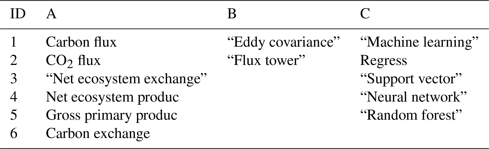
Table 1 Article search query design: “[A1 OR A2 OR A3, etc.] AND [B1 OR B2, etc.] AND [C1 OR C2, etc.]”.

The spatio-temporal heterogeneity of datasets and validation method. The spatio-temporal heterogeneity of the dataset may affect model accuracy. Typically, training data with larger regions, multiple sites, multiple PFTs, and longer spans of years may have a higher degree of imbalance (Kaur et al., 2019; Van Hulse et al., 2007; Virkkala et al., 2021; Zeng et al., 2020). Modeling with unbalanced data (where the difference between the distribution of the training and validation sets is significant even if selected at random) may result in lower model accuracy. To date, the most commonly used methods for validating such models include spatial (Virkkala et al., 2021), temporal (Reed et al., 2021), and random (Cui et al., 2021) cross-validation. The imbalance of data between the training and validation sets may affect the accuracy of the models when using these validation methods. Spatial validation is used to assess the ability of the model to adapt to different regions or flux sites of different PFTs, and a common method is “leave-one-site-out” cross-validation (Virkkala et al., 2021; Zeng et al., 2020). If the data from the site left out are not covered (or only partially covered) by the distribution of the training dataset, the model's prediction performance at that site may be poor due to the absence of a similar type in the training set. Temporal validation typically uses some years of data as training and the remaining years as validation to assess the model's fitness for interannual variability. For a year that is left out (e.g., a special extreme drought year which does not occur in the training set), the accuracy of the model may be limited if there are no similar years (extreme drought years) in the training dataset. K-fold cross-validation is commonly used in random cross-validation to assess the fitness of the model with regards to the spatio-temporal variability. In this case, different values of K may also have a significant impact on the model accuracy. For example, for an unbalanced dataset, the average model accuracy obtained from a 10-fold (K=10) validation approach is likely to be higher than that of a 3-fold (K=3) validation approach (Marcot and Hanea, 2021).

Machine learning algorithms used. Simulating NEE using different machine learning algorithms may influence the model accuracy, which may be induced by the characteristics of these algorithms themselves and the specific data distribution of the NEE training set. For example, neural networks can be used effectively to deal with nonlinearities, while as an ensemble learning method, random forests can avoid overfitting due to the introduction of randomness. Therefore, a comprehensive evaluation of this is necessary.

In this study, to evaluate the impacts of predictor use, algorithms, spatial scale/timescale, and validation methods on model accuracy, we performed a meta-analysis of papers with prediction models that combine NEE observations from flux towers, various predictors, and machine learning for the data-driven NEE simulations. In addition, we also analyzed the causality of multiple features in NEE simulations and the joint effects of multiple features on model accuracy using the Bayesian network (BN) (a multivariate statistical analysis approach; Pearl, 1985). The findings of this study can provide some general guidance for future NEE simulations.

2 Methodology

2.1 Criteria for including articles

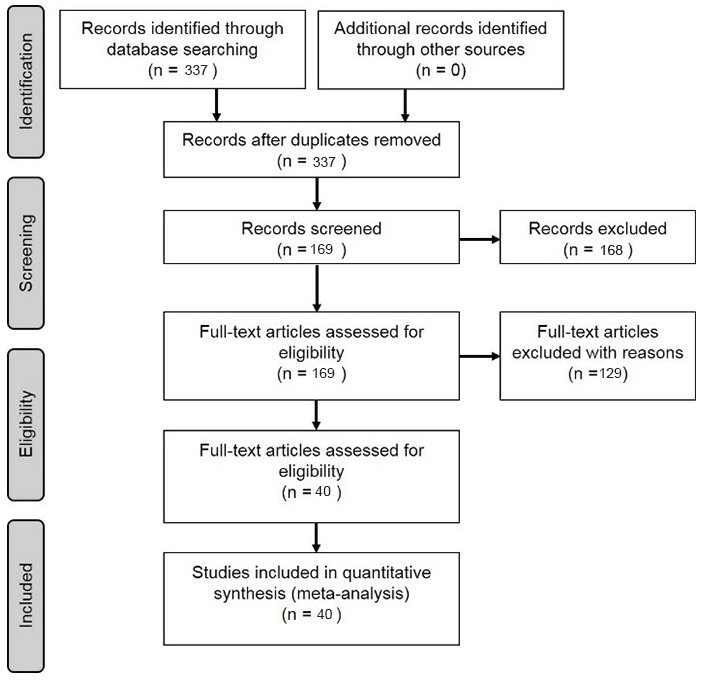
In the Scopus database, a literature query was applied to titles, abstracts, and keywords (Table 1) according to preferred reporting items for systematic reviews and meta-analyses (PRISMA) guidelines (Moher et al., 2009) (Fig. 1):

• a.

  Articles were filtered for those that modeled NEE. Articles that modeled other carbon fluxes such as methane flux were not included.

• b.

  Articles that used only univariate regression rather than multiple regression were screened out.

• c.

  Articles reported the determination coefficient (R²) of the validation step (Shi et al., 2021; Tramontana et al., 2016; Zeng et al., 2020) as the measure of model performance. Although RMSE is also often used for model accuracy assessment, its dependence on the magnitude of water flux values makes it difficult to use for fair comparisons between studies.

• d.

  Articles were published in journals with language limited to English.

• e.

  Articles were filtered for those that were published in specific journals (Table S1 in the Supplement) for research quality control because the data, model implementation, and peer review in these journals are often more reliable.

Figure 1 PRISMA-based paper filtering flowchart.

2.2 Features of prediction models

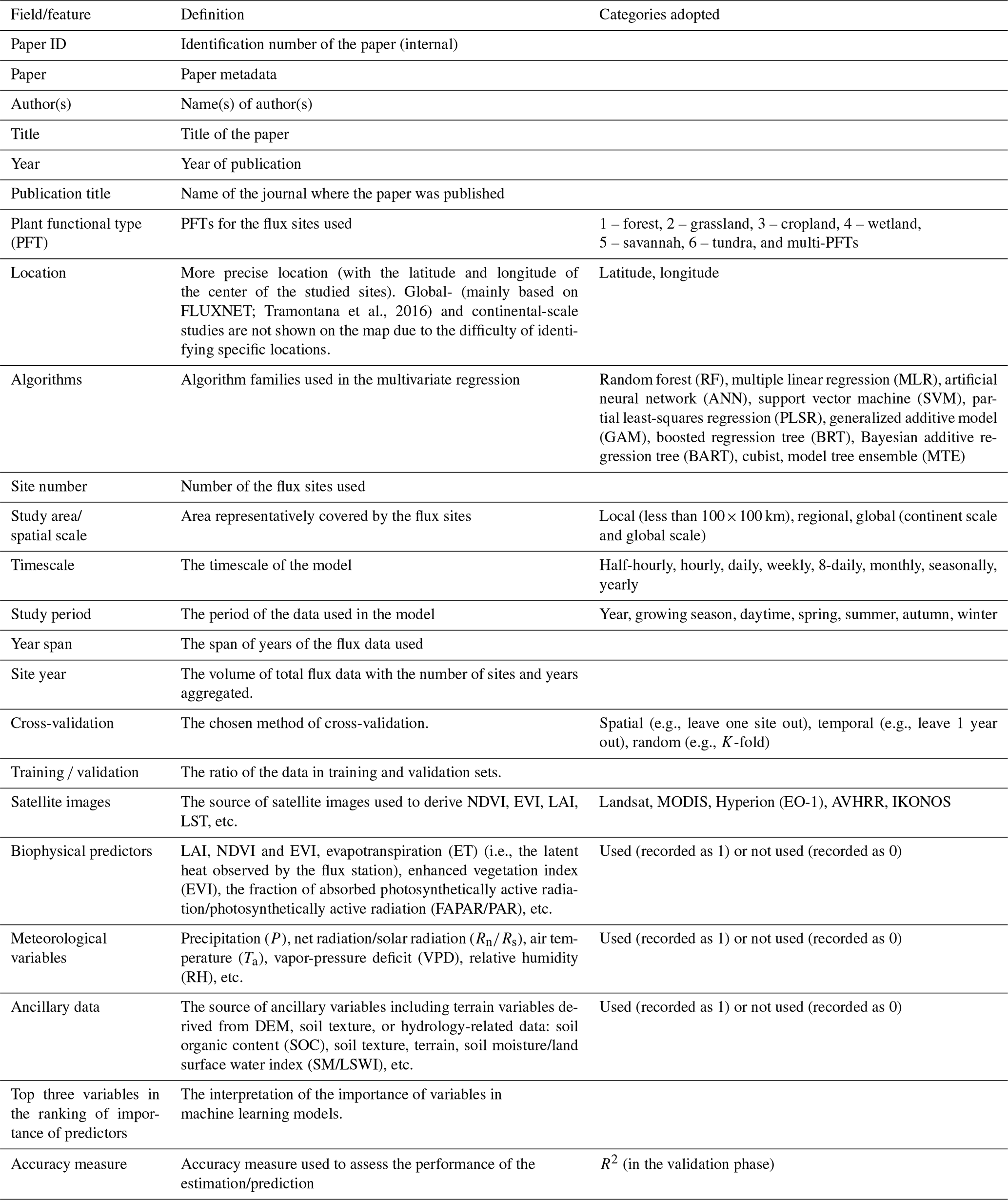
Typically, the flow of the NEE prediction modeling framework (Fig. 2) based on flux observations and machine learning is as follows: first, half-hourly scale NEE flux observations are aggregated into various timescale NEE data, and gap-filling techniques (Moffat et al., 2007) are often used in this step to obtain complete NEE series when data are missing. Various predictors including meteorological variables, remote-sensing-based biophysical variables, etc. are extracted to match site-scale NEE series to generate a training dataset containing the target variable NEE and various covariates. Subsequently, various algorithms are used for the NEE prediction model construction and validated in different ways (e.g., leave-one-site-out validation; Zeng et al., 2020). Finally, in some studies, prediction models were applied to gridded covariate data to map the regional- or global-scale NEE spatial and temporal variations (Zeng et al., 2020; Papale and Valentini, 2003; Jung et al., 2020). The information of R² (at the validation phase) and the associated model features reported in the article are considered one data record for the formal meta-analysis (i.e., each R² record corresponding to a prediction model). From the included papers, R² records and various features (Table 2) involved in the NEE modeling framework (Fig. 2) were extracted (including the algorithms used, modeling/validation methods, remote sensing data, meteorological data, biophysical data, and ancillary data). In some studies, multiple algorithms were applied to the same dataset or models with different features were developed (Virkkala et al., 2021; Zhang et al., 2021; Cleverly et al., 2020; Tramontana et al., 2016). In these cases, multiple data records will be documented.

In the practical information-extracting step, we categorized such features in a comparable manner. First, we categorized the various algorithms used in these papers, although the same algorithm may also have a variant form or an optimized parameter scheme. They are categorized into the following families of algorithms: random forest (RF), multiple linear regression (MLR), artificial neural network (ANN), support vector machine (SVM), partial least-squares regression (PLSR), generalized additive model (GAM), boosted regression tree (BRT), Bayesian additive regression tree (BART), cubist, and model tree ensemble (MTE). Second, we classified the spatial scales of these studies. Models with study areas (spatial extent covered by flux stations) smaller than 100×100 km were classified as “local”-scale models; those with study area sizes exceeding the continental scale were classified as “global” scale; and those with study area sizes in between were classified as “regional” scale. Third, for various predictors, we only recorded whether the predictors were used or not without distinguishing the detailed data sources and categories (e.g., grid meteorological data from various reanalysis datasets and in situ meteorological observations from flux stations), measurement methods (e.g., soil moisture measured/estimated by remote sensing or in situ sensors), etc. Fourth, we documented PFTs for the prediction models from the description of study areas or sites in these papers. They are classified into the following types: forest, grassland, cropland, wetland, savannah, tundra, and multi-PFTs (models containing a mixture of multiple PFTs). Models not belonging to the above PFTs were not given a PFT field and were not included in the subsequent analysis of the PFT differences. Other features (Table 2) are extracted directly from the corresponding descriptions in the papers in an explicit manner.

Subsequently, the model accuracies corresponding to different levels of various features are compared in a cross-study fashion. In the evaluation of algorithms and timescales, we also implement comparisons within individual studies. For example, in the evaluation of the effects of the algorithms, we compare the accuracy of models using the same training data and keeping other features as constants in individual studies. In this intra-study comparison step, only algorithms with relatively large sample sizes in the cross-study comparisons were selected. In this study, algorithms with fewer than 10 available model records are not considered to have a sufficient sample size and we do not give further conclusive opinions on the accuracy of these algorithms due to their small samples (e.g., PLSR and BART with high R² but very few records as evidence). MLR, RF, SVM, and ANN algorithms were found to have large sample sizes (Fig. 5a), and thus their accuracies can be comparable. Based on this, in the intra-study comparison step, we only compare the accuracy differences between MLR, RF, SVM, and ANN algorithms in the context of using the same data and the same other model features (Fig. 5b).

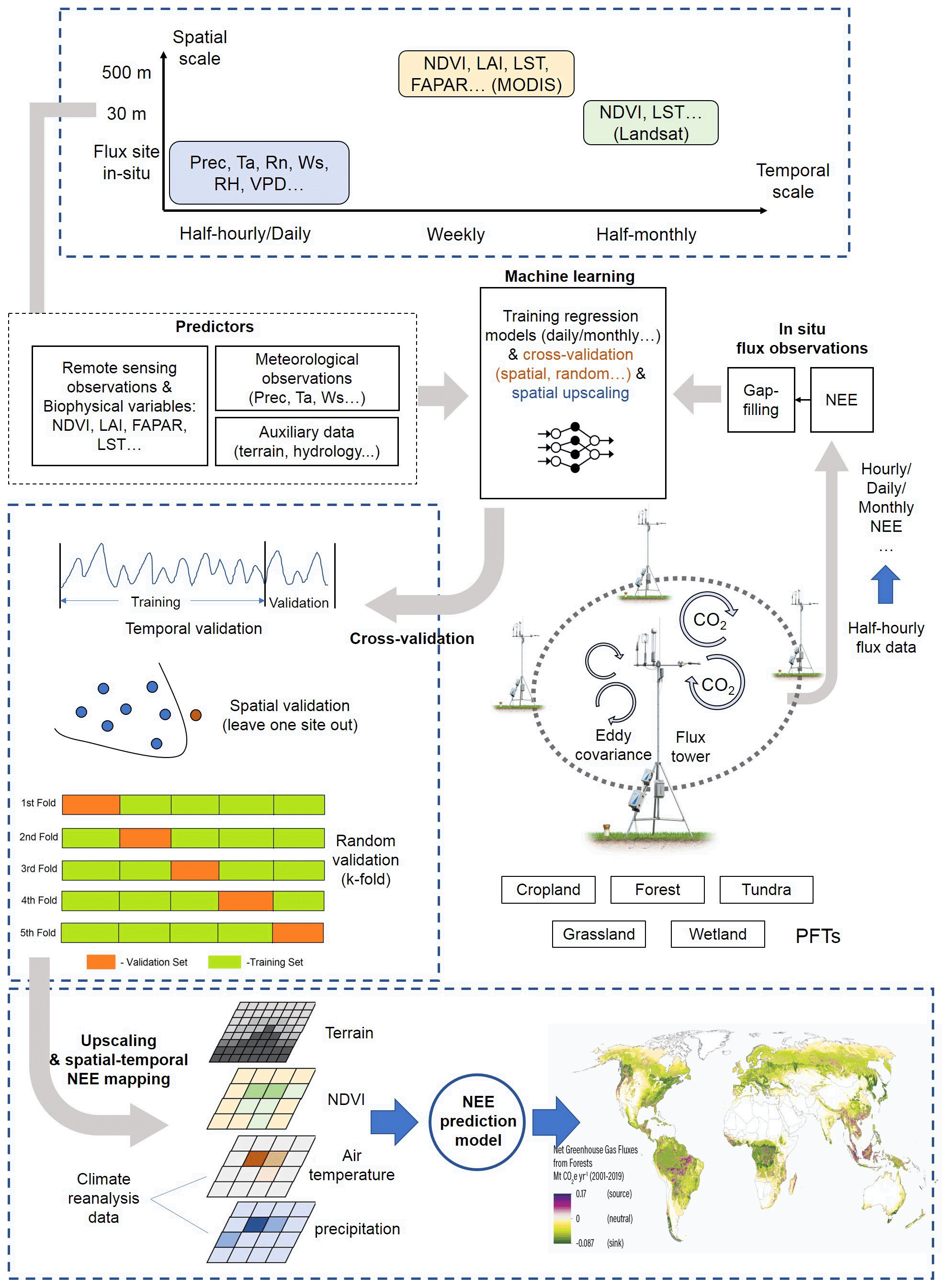
Figure 2 Features of the machine-learning-based NEE prediction process. The flux tower photo is from https://www.licor.com/env/support/Eddy-Covariance/videos/ec-method-02.html (last access: 23 March 2022). The map in the lower part is from Harris et al. (2021). P, T_a, R_n, W_s, RH, and VPD represent precipitation, air temperature, net surface radiation, wind speed, relative humidity, and vapor-pressure deficit, respectively. FAPAR is the fraction of absorbed photosynthetically active radiation. LST is the land surface temperature. LAI is the leaf area index.

Table 2 Description of information extracted from the included papers.

2.3 Bayesian network for analyzing joint effects

Based on the Bayesian network (BN), the joint impacts of multiple model features on the R² are analyzed. A BN can be represented by nodes (X₁, X_n) and the joint distribution (Pearl, 1985):

$$\begin{array}{}\text{(1)}& P\left(X\right)=P\left(X_{\mathrm{1}},X_{\mathrm{2}},\mathrm{\dots },X_n\right)=\prod _{i=\mathrm{1}}^{n}P\left(X_i|\mathrm{pa}\left(X_i\right)\right),\end{array}$$

where pa(X_i) is the probability of the parent node X_i. The expectation–maximization (EM) approach (Moon, 1996) is used to incorporate the collected model records and compile the BN.

Sensitivity analysis is used for the evaluation of node influence based on mutual information (MI), which is calculated as the entropy reduction of the child node resulting from changes at the parent node (Shi et al., 2020):

$$\begin{array}{}\text{(2)}& \begin{array}{rl}\mathrm{MI}=& H\left(Q\right)-H\left(Q\left|F\right.\right)\\ =& {\sum }_q{\sum }_{f}P\left(q,f\right){\log }_{\mathrm{2}}\left({\displaystyle \frac{P\left(q,f\right)}{P\left(q\right)P\left(f\right)}}\right)\end{array},\end{array}$$

where H represents the entropy, Q represents the target node, F represents the set of other nodes, and q and f represent the status of Q and F.

3 Results

3.1 Articles included in the meta-analysis

We included 40 articles (Table S2) and extracted 178 model records for the formal meta-analysis (Fig. 1). Most studies were implemented in Europe, North America, Oceania, and China (Fig. 3). The number of such papers has been increasing recently (Fig. 4), and it can be seen that the machine learning approach for NEE prediction has recently been of interest to more researchers. The main journals in which these articles have been published (Fig. 4) include Remote Sensing of Environment, Global Change Biology, Agricultural and Forest Meteorology, Biogeosciences, and Journal of Geophysical Research: Biogeosciences.

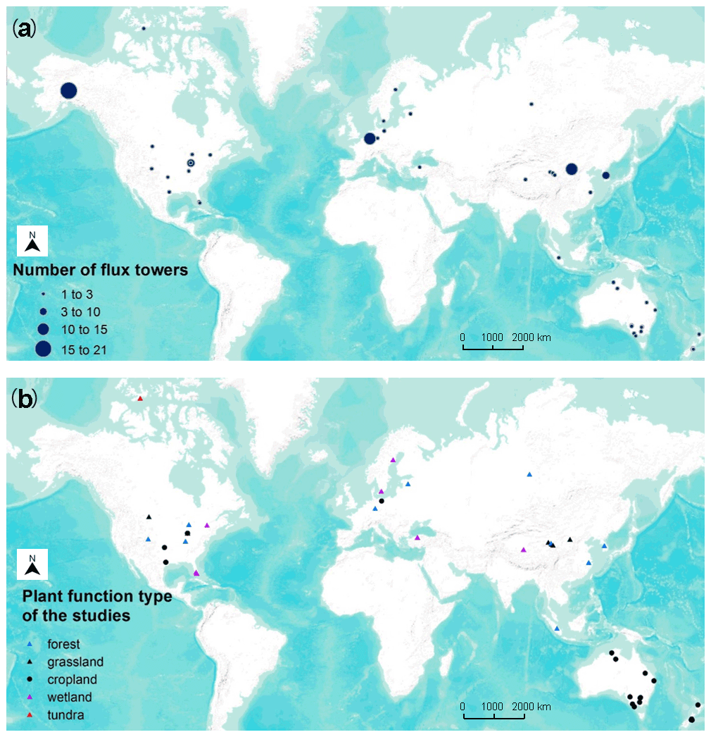
Figure 3 Location of studies (a) with the number of flux sites included and (b) their PFTs in the meta-analysis (total of 40 studies and 178 model records). Global- (mainly based on FLUXNET; Tramontana et al., 2016) and continental-scale studies are not shown on the map due to the difficulty of identifying specific locations.

3.2 The formal meta-analysis

We assessed the impact of the features (e.g., algorithms, study area, PFTs, number of data, validation methods, predictor variables) used in the different models based on differences in R².

3.2.1 Algorithms

Among the more frequently used algorithms, ANN and SVM algorithms performed better (Fig. 5a) on average across studies (slightly better than RF). On the other hand, since cross-study comparisons of algorithm accuracy include differences in data used in model construction, we performed a pairwise comparison (Fig. 5b) of these four algorithms (i.e., ANN, SVM, RF, and MLR). In these studies, multiple models are developed for consistent training data with the interference of training data differences removed. It shows that RF and SVM algorithms perform best in the inter-study comparison (Fig. 5b). Whereas the ANN category performed slightly worse than RF and SVM, all three of them were stronger than MLR. Overall, the performance of RF and SVM algorithms may be good and similar in the NEE simulations.

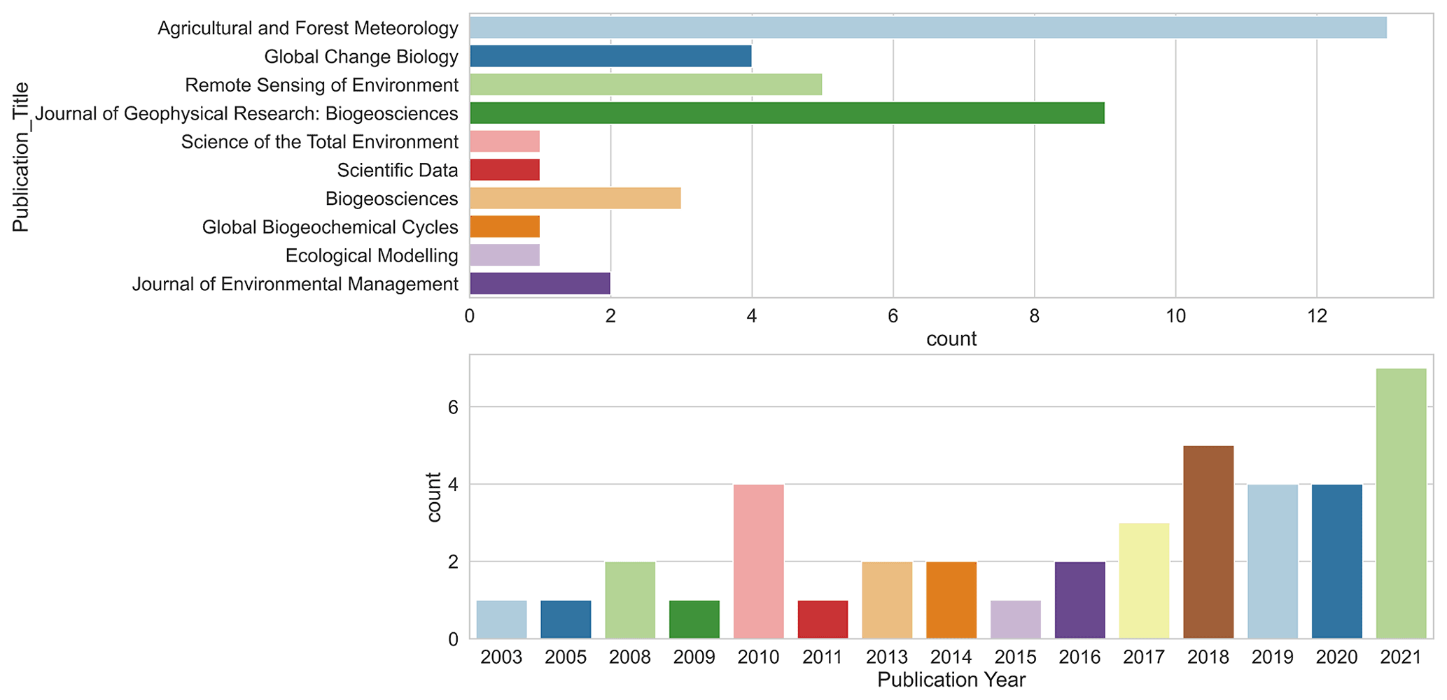
Figure 4 The number of studies published across journals and the total number of publications per year.

3.2.2 Timescales

The impact of timescale on R² is considerable (Fig. 6), with models with larger timescales having lower average R², especially when the timescale exceeds the monthly scale. The most frequently used scales were the daily, 8 d, and monthly scales. In studies where multiple timescales were used with other characteristics being the same, we found that models with half-hourly scales were significantly more accurate than models with daily scales (Fig. 6). However, the difference in accuracy between the day-scale and week-scale models is small. The accuracy of models with a monthly scale is the lowest.

3.2.3 Various predictors

Among the commonly used predictors for NEE, there are significant differences in the predictors used and their impacts on model accuracy for different PFTs (Fig. 7). Ancillary data (e.g., soil texture, soil organic content, topography) that do not have temporal variability are used less frequently because they can only explain spatial heterogeneity. In contrast, the biophysical variables LAI, FAPAR, and ET were used significantly less frequently than NDVI and EVI, especially in the cropland and wetland types. The meteorological variables T_a, $R_{\text{n}}/R_{\text{s}}$, and VPD were used most frequently. For forest sites, $R_{\text{n}}/R_{\text{s}}$ and W_s appear to be the variables that improve model accuracy. For grassland sites, we found that NDVI and EVI appear to be the most effective, despite the small sample size. For sites in croplands and wetlands, we did not find predictor variables that had a significant impact on model accuracy.

For different PFTs, the top three variables in the ranking of model importance differed (Fig. S1 in the Supplement). SM, $R_{\text{n}}/R_{\text{s}}$, T_a, T_s, and VPD all showed high importance across PFTs. This suggests that the variability in measured site-scale moisture and temperature conditions is important for the simulation of NEE for all PFTs. In contrast, in the importance ranking, other variables such as precipitation and NDVI and EVI may not lead because of the lag in their effect on NEE (Hao et al., 2010; Cranko Page et al., 2022). And some other variables may improve model accuracy for specific PFTs such as groundwater table depth (GWT) for wetland sites and growing degree days (GDDs) for tundra sites.

3.2.4 Other features

In addition, we evaluated other features of the model construction that may contribute to differences in model accuracy (Fig. 8). Studies at continental and global scales with a large number of sites and a large span of years correspond to lower R² values than studies at local and regional scales, suggesting that studies with a large number of sites across large regions are likely to have high variability in the relationship between NEE and covariates and that studies at small scales are more likely to have higher model accuracy. Spatial validation (usually leave one site out) corresponds to lower model accuracy compared to random and temporal validation. This again confirms the dominant role of heterogeneity in the relationship between NEE and covariates across sites in explaining model accuracy. This seems to be indirectly supported by the fact that a high ratio of training to validation sets corresponds to a low R² as this high ratio tends to be accompanied by the use of the leave-one-site-out validation approach. The accuracy of the models with a growing season period was slightly higher than that of the models with an annual period. For the satellite remote sensing data used, the models based on MODIS data with biophysical variables extracted were slightly less accurate than those based on Landsat data. For the daily scale models, Landsat data performed a little better than MODIS (Fig. S2). This suggests that the higher temporal resolution of MODIS compared to Landsat may not play a dominant role in improving model accuracy. This may also be partially attributed to studies using MODIS-based explanatory data that tend to include too large surrounding areas around the site (e.g., 2×2 km), which can lead to a scale mismatch between the flux footprint and the explanatory variables.

3.3 The joint causal impacts of multi-features based on the BN

We selected the features that had a more significant impact on model accuracy in the above assessment and further incorporated them into the BN-based multivariate assessment to understand the joint impact of multiple features on R². The features incorporated included the spatial scale, the number of sites, the timescale, the span of years, the cross-validation method, and whether some specific predictors were used. We discretized the distribution of individual nodes and compiled the BN (Fig. 9a) using records from different PFTs as input. Sensitivity analysis of the R² node (Fig. 10) showed that R² was most sensitive to “year span”, the cross-validation method, $R_{\text{n}}/R_{\text{s}}$, and the timescale under multi-feature control. In the forest and cropland types, R² is more sensitive to $R_{\text{n}}/R_{\text{s}}$, while in the wetland type it is more sensitive to SM and LSWI and T_a. The sensitivity of R² to year span was much higher in the cropland type compared to the other PFTs, which may suggest that the interannual variability in the NEE simulations of the cropland type is higher due to potential interannual variability in the planting structure and irrigation practices. For the cropland type, differences in the phenology, harvesting, and irrigation (water volume and frequency) in different years can lead to significant interannual differences in NEE simulations. Subsequently, using the constructed BN (with the empirical information in previous studies incorporated), for new studies we can instructively infer the probability distribution of the possible R² (Fig. 9b) with some model features predetermined. In previous studies, spatio-temporal mapping of NEE based on statistical models has often lacked accuracy assessment since there are no grid-scale NEE observations, and this BN may have the potential to be used to validate the accuracy (R²) of the NEE time series output of the grid scale (i.e., inferring possible R² values from model features, where the output of the grid scale is considered to be of the form leave one site out).

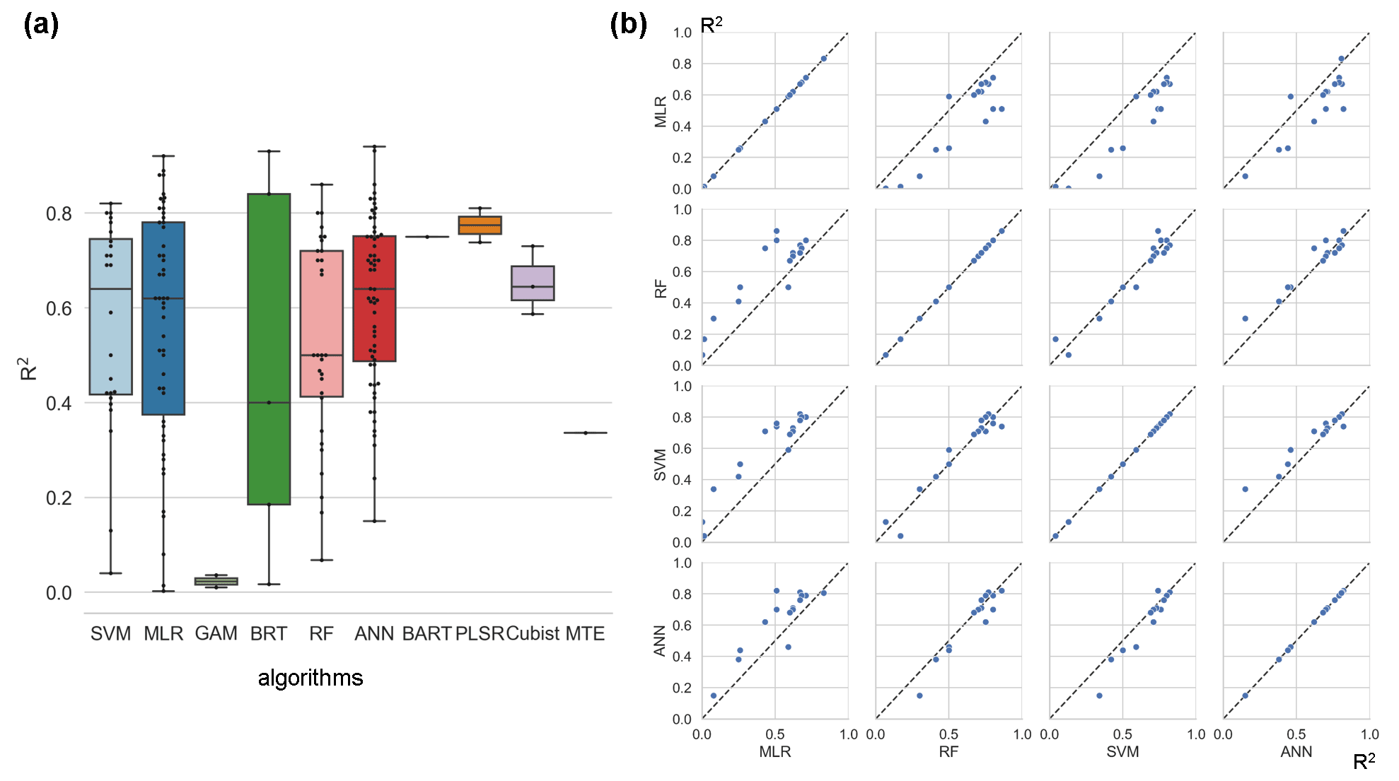
Figure 5 Differences in model accuracy (R²) using different algorithms across studies (a) and internal comparisons of the model accuracy (R²) of selected pairs of algorithms within individual studies (b). Regression algorithms: random forest (RF), multiple linear regression (MLR), artificial neural network (ANN), support vector machine (SVM), partial least-squares regression (PLSR), generalized additive model (GAM), boosted regression tree (BRT), Bayesian additive regression tree (BART), cubist, model tree ensemble (MTE). In (a) the horizontal line in the box indicates the medians. The top and bottom border lines of the box indicate the 75th and 25th percentiles, respectively.

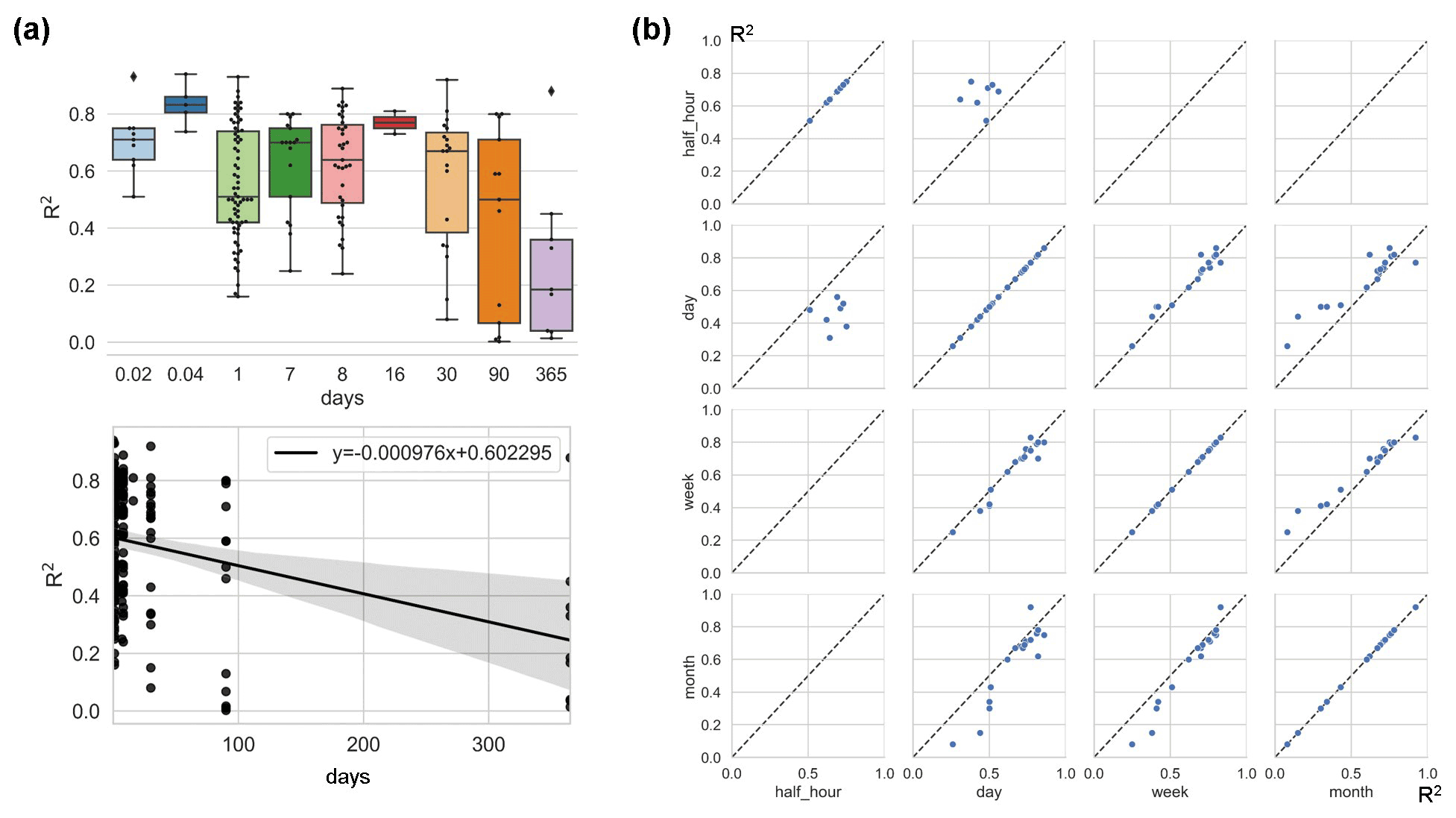
Figure 6 Differences in model accuracy (R²) at different timescales across studies with the linear regression between R² and timescales (a) and comparison of the model accuracy (R²) of selected pairs of timescales within individual studies (b). All model records were included in (a), while studies that used multiple timescales (with other model characteristics unchanged) were included in (b). Timescales: 0.02 d (half-hourly), 0.04 d (hourly), 30 d (monthly), and 90 d (quarterly).

4 Discussions

Many studies have evaluated the incorporation of various predictors and model features using machine learning for improving the site-scale NEE predictions (Tramontana et al., 2016; Zeng et al., 2020; Jung et al., 2011). A comprehensive evaluation of these studies to provide definitive guidance on the selection of features in NEE prediction modeling is limited. This study fills the research gap with a meta-analysis of the literature through statistics on the accuracy and performance of models. Machine-learning-based NEE simulations and predictions still suffer from high uncertainty. By better understanding the expected improvements that can be achieved through the inclusion of different features, we can identify priorities for the consideration of different features in modeling efforts and avoid operations decreasing model accuracy.

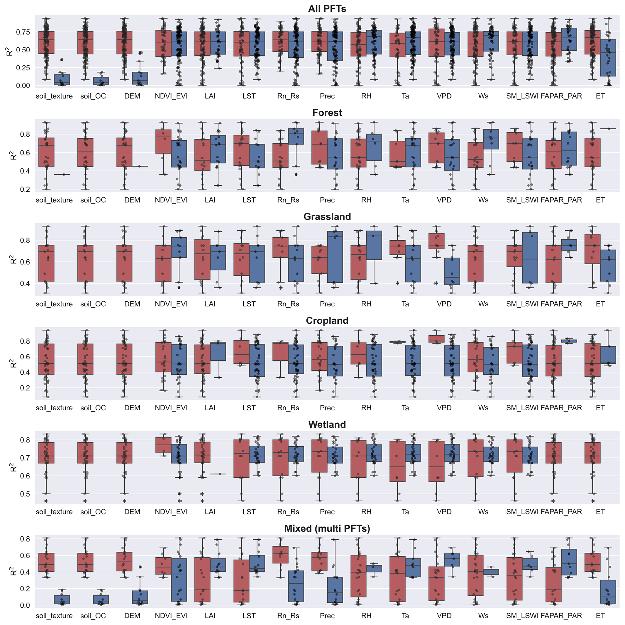
Figure 7 The impact of the various predictors incorporated in models of different PFTs on R². Dark blue boxes indicate that the predictor was used in the model, while dark red boxes indicate that the predictor was not used. Predictors: soil organic content (soil_OC), precipitation (P), soil moisture and land surface water index (SM_LSWI), net radiation/solar radiation (R_n_R_s), enhanced vegetation index (EVI), air temperature (T_a), vapor-pressure deficit (VPD), the fraction of absorbed photosynthetically active radiation/photosynthetically active radiation (FAPAR_PAR), relative humidity (RH), evapotranspiration (ET), leaf area index (LAI).

Compared to previous comparisons of machine-learning-based NEE prediction models, this study is more comprehensive. Previous studies (Abbasian et al., 2022) have also found advantages of RF over other algorithms in NEE prediction. This study consolidated this finding using a larger amount of evidence. Previous studies (Tramontana et al., 2016) have also compared the impact of different practices in NEE prediction models based on R², such as comparing the difference in accuracy between the two predictor combinations (i.e., using only remotely sensed data and using remotely sensed data and meteorological data together). In contrast, since this study incorporated more detailed factors influencing model accuracy, the understanding of such issues was deepened. However, there are still many uncertainties and challenges in NEE prediction that have not been clarified in this study.

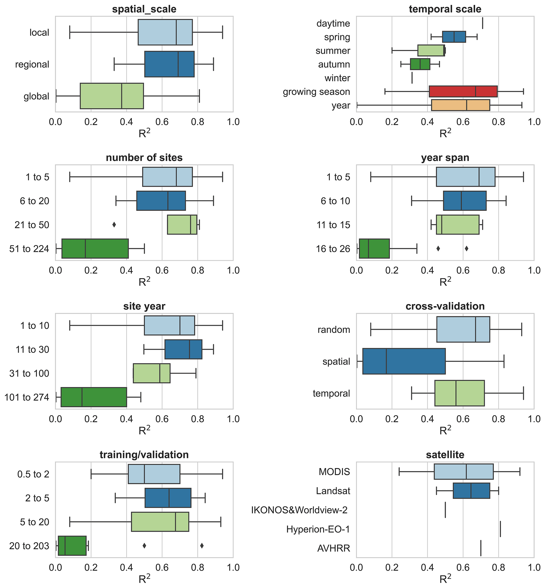
Figure 8 The impacts of other features (i.e., spatial scale, study period, number of sites, year span, site year, cross-validation method, training $/$ validation, and satellite imagery) on the model performance.

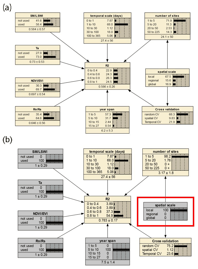
Figure 9 The joint effects of multiple features on R² based on the BN with all records input (a) and the inference on the probability distribution of R² based on the BN with the status of some nodes determined (b). The values before and after the “±” indicate the mean and standard deviation of the distribution, respectively. The gray boxes indicate that the status of the nodes has been determined. In (b), specific values of parent nodes such as “spatial scale” are determined (shown in the red box), leading to an increase in the expected R² compared to the average scenario of (a) (as inferred from the posterior conditional probabilities with the status of the node spatial scale determined as local).

4.1 Challenges of the site-scale NEE simulation and implications for other carbon flux simulations

4.1.1 Variations in timescales

In the above analysis, we found that the effect of the timescale of the model is considerable. This suggests that we should be careful in determining the timescale of the model to consider whether the predictor variables used will work at this timescale. Previous studies have reported the dependence of the NEE variability and mechanism on the timescales. On the one hand, the importance of variables affecting NEE varies at different timescales. For example, in tropical and subtropical forests in southern China (Yan et al., 2013), seasonal NEE variability is predominantly controlled by soil temperature and moisture, while interannual NEE variability is controlled by the annual precipitation variation. A study (Jung et al., 2017) showed that for annual-scale NEE variability, water availability and temperature were the dominant drivers at the local and global scales, respectively. This indicates the need to recognize the temporal and spatial driving mechanisms of NEE in advance in the development of NEE prediction models. On the other hand, dependence may exist between NEE anomalies at various timescales. For example, previous studies (Luyssaert et al., 2007) showed that short-term temperature anomalies may be interpreted as both the daily and the seasonal NEE anomalies. This implies that the models at different timescales may not be independent. In the previous studies, the relationship between prediction models at different scales has not been well investigated, and it may be valuable to compare the relations between data and models at different scales in depth. Larger timescales correspond to lower model accuracy, possibly related to the fact that some small-timescale relations between NEE and covariates (especially meteorological variables) are smoothed. In particular, for models with timescales smaller than 1 d (e.g., half-hourly models), the 8-daily and 16-daily biophysical variable data obtained from satellite remote sensing are difficult to use to explain the temporal variation in the sub-daily NEE. Therefore, for models at small timescales (i.e., half-hourly, hourly, daily scale models), in situ meteorological variables may be more important. The inclusion of some ancillary variables (e.g., soil texture, topographic variables) with no temporal dynamic information may be ineffective unless many sites are included in the model and the spatial variability in the ancillary variables for these sites is sufficiently large (Virkkala et al., 2021).

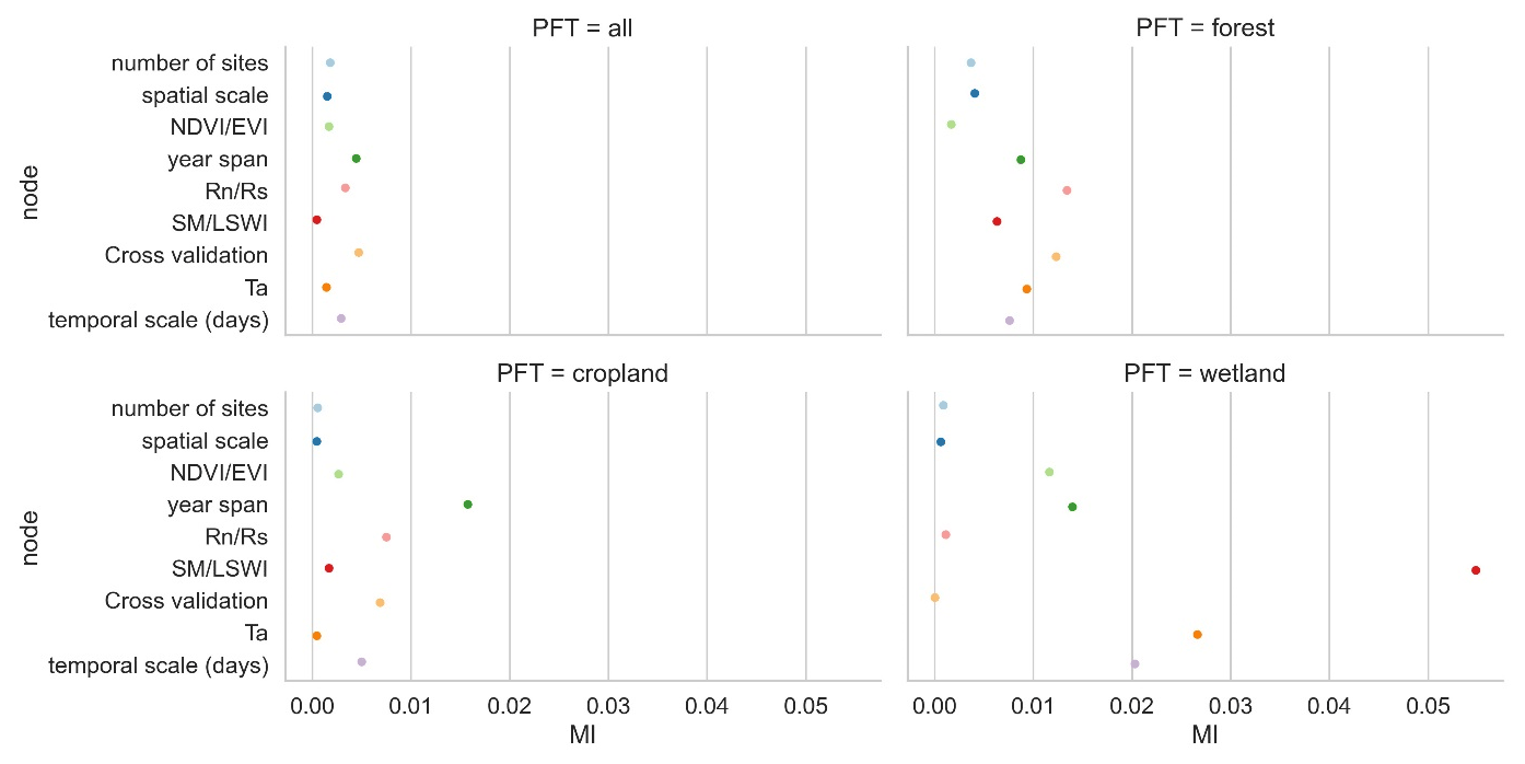
Figure 10 The sensitivity analysis of the R² node to other nodes based on the mutual information (MI) across PFTs. “Cross-validation” is the cross-validation method including spatial, temporal, and random cross-validation.

In terms of completeness and purity of training data, hourly and daily models can be better compared to monthly and yearly models. Hourly and daily models can usually preclude those low-quality data and gaps in the flux observations. However, for monthly and yearly scale models, gap filling (Ruppert et al., 2006; Moffat et al., 2007; Zhu et al., 2022) is necessary because there are few complete and continuous flux observations without data gaps on the monthly to yearly scales. Since various gap-filling techniques rely on environmental factors (Moffat et al., 2007) such as meteorological observations, this may introduce uncertainty into the predictive models (i.e., a small fraction of the observed information of NEE is estimated from a combination of independent variables). How it would affect the accuracy of prediction models at various timescales remains uncertain, although various gap-filling techniques have been widely used in the pre-processing of training data.

In addition, the impacts of lagged effects (Hao et al., 2010; Cranko Page et al., 2022) of covariates are not considered in most models, which may underestimate the degree of explanation of NEE for some predictor variables (e.g., precipitation). Most of the machine-learning-based models use only the average T_a and do not take into account the maximum temperature, minimum temperature, daily difference in temperature, etc. as in the process-based ecological models (Mitchell et al., 2009). This suggests that the inclusion of different temporal characteristics of individual variables in machine-learning-based NEE prediction models may be insufficient.

4.1.2 Scale mismatch of explanatory predictors and flux footprints

An excessively large extraction area of remote sensing data (e.g., 2×2 km) may be inappropriate. In the non-homogeneous underlying conditions, the agreement of the area of flux footprints with the scale of the predictors should be considered in the extraction of the predictor variables in various PFTs (Chu et al., 2021).

The effects of this mismatch between explanatory variables and flux footprints may be diverse for different PFTs. For example, for cropland types, the NEE is monitored at a range of several hundred meters around the flux towers, but remote sensing variables such as FAPAR, NDVI, or LAI can be extracted at coarse scales (e.g., 2×2 km) and some effects outside the extent of the flux footprint (Chu et al., 2021; Walther et al., 2021) are incorporated (e.g., planting structures with high spatial heterogeneity, agricultural practices such as irrigation). And for more homogeneous types such as grasslands, coarse-scale meteorological data may still cause spatial mismatches, even though the differences in land cover types within the 2×2 km and 200×200 m extent around the flux stations in grasslands may not be considerable. For example, precipitation with high spatial heterogeneity can dominate the spatial variability in soil moisture and thus affect the spatial variability in grassland NEE (Wu et al., 2011; Jongen et al., 2011). However, using ${\mathrm{0.25}}^{\circ }\times {\mathrm{0.25}}^{\circ }$ reanalysis precipitation data (Zeng et al., 2020) may make it difficult for predictive models to capture this spatial heterogeneity around the flux station.

Since few of the studies included in this meta-analysis considered the effect of variation in the flux footprint, this feature was difficult to consider in this study. However, its influence should still be further investigated in future studies. With flux footprints calculated (Kljun et al., 2015) and the factors around the flux site (Walther et al., 2021) that affect the flux footprint incorporated, it is promising to clarify this issue.

4.1.3 Possible unbalance of training and validation sets

In addition to the timescale of the models, the most significant differences in model accuracy and performance were found in the heterogeneity within the NEE dataset and the match of the training set and validation set. Often NEE simulations can achieve high accuracy in local studies, where the main factor negatively affecting model accuracy may be the interannual variability in the relationship between NEE and covariates. However, the complexity may increase when the dataset contains a large study area and many sites, PFTs, and year spans. Under this condition, the accuracy of the model in the leave-one-site-out validation may be more dependent on the correlation and match between the training and validation sets (Jung et al., 2020). When the model is applied to an outlier site (of which the NEE, covariates, and their relationship are very different compared with the remaining sites), it appears to be difficult to achieve a high prediction accuracy (Jung et al., 2020). If we further upscale the prediction model to large spatial scales and timescales, the uncertainties involved may be difficult to assess (Zeng et al., 2020). We can only infer the possible model accuracy based on the similarity of the distribution of predictors in the predicted grid to that of the existing sites in the model. In the upscaling process, reanalysis data with coarse spatial resolution are often used as an alternative for site-scale meteorological predictors. However, most studies did not assess in detail the possible errors associated with spatial mismatches in this operation.

In summary, the site-scale NEE predictions may require more focus on the internal heterogeneity of the NEE dataset and the matching of the training set and validation set and also require a better understanding of the influence of different scales of the same variable (e.g., site-scale precipitation and grid-scale precipitation in the reanalysis meteorological data) across modeling and upscaling steps. For the prediction of other carbon fluxes such as methane fluxes (in the same framework as the NEE predictions), the results of this study may also be partially applicable, although there may be significant differences in the use of specific predictors (Peltola et al., 2019).

4.2 Uncertainties

The uncertainties in this analysis may include the following:

• a.

  Publication bias and weighting. Publication bias is not refined due to the limitations of the number of articles that can be included. Meta-analyses often measure the quality of journals and the data availability (Borenstein et al., 2011; Field and Gillett, 2010) to determine the weighting of the literature in a comprehensive assessment. However, a high proportion of the articles in this study did not make flux observations publicly available or share the NEE prediction models developed. Furthermore, meta-analysis studies in other fields typically measure the impact of papers by evidence/data volume and the variance of the evaluated effects (Adams et al., 1997; Don et al., 2011; Liu et al., 2018). However, in this study, because no convincing method is found to quantify the weights of results from included articles, some features (e.g., the number of flux sites, the span of years) were directly assessed rather than used to determine the weights of the articles.

• b.

  Limitations of the criteria for inclusion in the literature. In the model-accuracy-based evaluation, we selected only literature that developed multiple regression models. Potentially valuable information from univariate regression models was not included. In addition, only papers in high-quality English journals were included in this study to control for possible errors due to publication bias. However, many studies that fit this theme may have been published in other languages or other journals.

• c.

  Independence between features. There is dependence between the evaluated features (e.g., the dependency between the spatial extent and the number of sites). This may negatively affect the assessment of the impact of individual features on the accuracy of the model, although the BN-based analysis of joint effects can reduce the impact of this dependence between variables by specifying causal relationships between features. The interference of unknown dependencies between features may still not be eliminated when we focus on the effects of an individual feature on the model performance. We should pay more attention to the effect of features on model accuracy individually in future studies, and it may be valuable to keep other features as constants while changing the level of only one feature and assessing the difference. This may help us to understand the real sensitivity of model accuracy to different features in specific conditions. The sample size collected in this study (178 records in total) is not very large. This also suggests that more efforts in future should be devoted to the comprehensive evaluation and summarization of NEE simulations.

• d.

  Other potential factors. Additionally, there are still other potential factors not considered by this study such as the uncertainty in climate data (site vs. reanalysis), footprint matching between site and satellite images, etc. Overall, although the quantitative results of this study should be used with caution, they still have positive implications for guiding such studies in the future.

5 Conclusions

We performed a meta-analysis of the site-scale NEE simulations combining in situ flux observations; meteorological, biophysical, and ancillary predictors; and machine learning. The impacts of various features throughout the modeling process on the accuracy of the model were evaluated. The main findings of this study include the following:

1. RF and SVM algorithms performed better than other evaluated algorithms.

2. The impact of timescale on model performance is significant. Models with larger timescales have lower average R² values, especially when the timescale exceeds the monthly scale. Models with half-hourly scales (average R² = 0.73) were significantly more accurate than models with daily scales (average R² = 0.5).

3. Among the commonly used predictors for NEE, there are significant differences in the predictors used and their impacts on model accuracy for different PFTs.

4. It is necessary to focus on the potential imbalance between the training and validation sets in NEE simulations. Studies at continental and global scales (average R² = 0.37) with multiple PFTs, more sites, and a large span of years correspond to lower R² values than studies at local (average R² = 0.69) and regional (average R² = 0.7) scales.