Local-scale evaluation of the simulated interactions between energy, water and vegetation in ISBA, ORCHIDEE and a diagnostic model

The processes involved in the exchange of water, energy and carbon in terrestrial ecosystems are strongly intertwined. To accurately represent the terrestrial biosphere in land surface models (LSMs), the intrinsic coupling between these processes is required. Soil moisture and leaf area index (LAI) are two key variables at the nexus of water, energy and vegetation. Here, we evaluated two prognostic LSMs (ISBA and ORCHIDEE) and a diagnostic model (based on the LSA SAF, Satellite Application Facility for Land Surface Analysis, algorithms) in their ability to simulate the latent heat flux (LE) and gross primary production (GPP) coherently and their interactions through LAI and soil moisture. The models were validated using in situ eddy covariance observations, soil moisture measurements and remote-sensing-based LAI. It was found that the diagnostic model performed consistently well, regardless of land cover, whereas important shortcomings of the prognostic models were revealed for herbaceous and dry sites. Despite their different architecture and parametrization, ISBA and ORCHIDEE shared some key weaknesses. In both models, LE and GPP were found to be oversensitive to drought stress. Though the simulated soil water dynamics could be improved, this was not the main cause of errors in the surface fluxes. Instead, these errors were strongly correlated to errors in LAI. The simulated phenological cycle in ISBA and ORCHIDEE was delayed compared to observations and failed to capture the observed seasonal variability. The feedback mechanism between GPP and LAI (i.e. the biomass allocation scheme) was identified as a key element to improve the intricate coupling between energy, water and vegetation in LSMs.

1 Introduction

Terrestrial ecosystems modulate the surface fluxes of heat, water and carbon and are thereby an essential driver of weather and climate (Pielke et al., 1998). They are a substantial dynamic component of the global carbon budget, with 15 % of the global atmospheric CO₂ being exchanged yearly through the stomata of leaves and assimilated through photosynthesis (IPCC, 2013). Furthermore, the pivotal role of vegetation in the global climate is mediated by its impact on the hydrological cycle (Falkenmark et al., 2004). Despite its importance in the framework of the globally changing climate, large uncertainties remain in our understanding of the coupling of the energy, water and carbon cycle in the terrestrial biosphere (Piao et al., 2013; De Kauwe et al., 2017; IPCC, 2019).

Land surface models (LSMs) are key tools to quantify these surface fluxes and to better the representation of their interactions. They allow the coupled simulation of the fluxes of water, energy and carbon between the surface and the atmosphere and are a crucial component of numerical weather models and earth system models. Over the past decades, they have evolved from their initial simple biophysical configuration to include more complex feedback mechanisms, such as soil moisture dynamics, dynamic vegetation and plant phenology (Delire et al., 2020; Fisher and Koven, 2020).

The processes involved in the surface fluxes from the terrestrial biosphere, such as photosynthesis, transpiration, soil hydrology and leaf phenology, are deeply intertwined with each other. Soil moisture and leaf area index (LAI) are two key variables at the nexus between energy, water and vegetation processes.

Root zone soil moisture affects the leaf exchange of water and carbon by modulating the stomatal closure (Raschke, 1979). Although the physiological processes involved are well described, there is a substantial disagreement in the stomatal behaviour across various models (De Kauwe et al., 2017). An evaluation of the impact of soil moisture in the CMIP5 models (Taylor et al., 2012) indicated that the LSMs were generally oversensitive to drought stress and wet events (Huang et al., 2016). Whereas several other studies have reported similar outcomes (Piao et al., 2013; Kolus et al., 2019), Rebel et al. (2012) found an underestimation of ORCHIDEE response to drought. Some of the key challenges lie in the upscaling of leaf-level processes to canopy-scale and ecosystem-scale simulations (De Kauwe et al., 2017); the broad range of processes contributing to evapotranspiration (ET), along with numerous feedback mechanisms (Bonan et al., 2014; Fisher and Koven, 2020); and the difficulty to simulate soil moisture dynamics and infiltration itself (Li et al., 2018; Vereecken et al., 2019). Furthermore, the validation of these simulations is hampered due to the scale mismatch between flux footprint and model grid and the challenge in accurately observing the partitioning of the surface fluxes (transpiration, soil evaporation, canopy intercept evaporation, etc.; Nelson et al., 2020).

Leaf area index is another key variable in terrestrial ecosystem models. It is used to represent the abundance of foliar vegetation and its canopy state. Many leaf-scale processes are scaled to canopy-scale surface fluxes, proportional to LAI. Over the past decades, simulations with prognostic LAI have become an established approach to account for interseasonal variability in the terrestrial vegetation in land surface models (Calvet et al., 1998; Dickinson et al., 1998; Krinner et al., 2005; Gibelin et al., 2006). The coupling of the carbon assimilation to a biomass allocation scheme allows the simulation of the variable phenological cycle and the vegetation response to atmospheric forcings. The degree of complexity of this scheme is very variable amongst models and ranges from fairly simplistic (e.g. in ISBA, Le Moigne et al., 2018, or CHTESSEL, Boussetta et al., 2013) to advanced, with dedicated phenology modules or non-structural carbohydrate dynamics (e.g. in ORCHIDEE, Krinner et al., 2005; CLM, Lawrence et al., 2019; or CLASS, Asaadi et al., 2018). Previous studies have concluded that LSMs are capable of representing the amplitude of the seasonal LAI cycle with reasonable accuracy (Gibelin et al., 2008), but substantial shortcomings are found in the timing of the phenological cycle and the interseasonal variability (Lafont et al., 2012). The disagreement amongst models (and observations) can be attributed to our limited knowledge of the drivers of budburst and senescence, biomass allocation, reserve dynamics, and belowground processes (Le Roux et al., 2001; Fatichi et al., 2019). As a consequence of the coupling of the vegetation dynamics with the water and carbon cycles, the uncertainty associated with the seasonal cycle of LAI propagates back to the surface fluxes.

The resulting feedbacks from the coupling are summarized in Fig. 1. Soil moisture and LAI are state variables which determine the exchange of heat, water and carbon. Through the feedback to soil moisture in prognostic models, uncertainties in the exchange of heat and water (e.g. sensible heat flux, H; latent heat flux, LE; or evapotranspiration) propagate to the carbon assimilation. Inversely, uncertainties in gross primary production (GPP) or the vegetation growth affect the heat and water fluxes over LAI. Finally, through phenology equations in some models (e.g. ORCHIDEE for grass), soil moisture can also affect LAI directly.

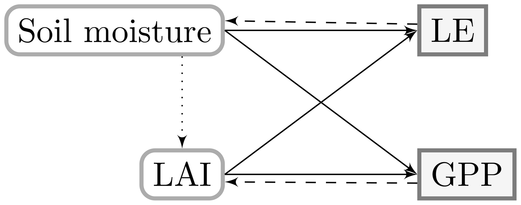
Figure 1 First-order relations (plain lines) and feedbacks (dashed lines) of the state variables and surface fluxes in prognostic LSMs. The feedback mechanisms are not present in diagnostic models, and the soil moisture–LAI relation (dotted line) occurs only in prognostic LSMs with dedicated phenology schemes.

This study focuses on the representation of these interactions in two well-established prognostic LSMs – ORCHIDEE (Krinner et al., 2005) and ISBA (Le Moigne et al., 2018) – and one diagnostic model (Ghilain et al., 2011; Martínez et al., 2020). The evaluation of LSMs is typically achieved by validating components of the LSMs individually, as mediated by the ever-increasing availability of long-term in situ measurements of energy, water and carbon fluxes from eddy covariance (EC) tower networks (Balzarolo et al., 2014; Napoly et al., 2017; Dirmeyer et al., 2018). In situ observations of surface fluxes, meteorological conditions and soil moisture are an essential resource in the study of terrestrial ecosystems and the development of LSMs. In combination with remote-sensing-based observations of LAI, they provide key insights in the interactions between the surface fluxes and the biosphere.

Beyond the validation of the model outputs, the assessment of the model dynamics and internal interactions is needed to further advance LSM development. Approaches to tackle this include sensitivity analyses, anomaly analysis or isolation of extreme events (e.g. Alton, 2016; Huang et al., 2016). Additionally, the quality of the prognostic state variables can be assessed through a functional evaluation. Here, the diagnostic LSM is used as a vehicle to test the impact of the prognostic soil moisture and LAI on the surface fluxes. Diagnostic LSMs are typically designed to estimate fluxes from observed state variables, such as remote-sensing-based soil moisture and LAI. Replacing the observed states by the prognostic states allows their impact on the surface fluxes to be tested. To our knowledge, this is the first study to perform such a functional evaluation of LSMs.

The objective of this paper is to evaluate the performance and internal dynamics of three LSMs at the local scale. Our focus is the relation between the surface fluxes (LE, GPP) and important state variables (soil moisture, LAI). This is done by (1) validation and intercomparison of the simulated surface fluxes and prognostic states in these models, (2) comparison of the model dynamics (phenology and flux partitioning), and (3) evaluation of the interactions with soil moisture and LAI. Given the degree of coupling in the current LSM, we try to disentangle the relation between key facets of the terrestrial vegetation in a holistic way.

2 Materials and methods

2.1 Models

Three well-established models were used to simulate the intrinsically coupled fluxes of water, energy and carbon from terrestrial vegetation: a diagnostic model based on the LSA SAF (Satellite Application Facility for Land Surface Analysis) algorithms (hereafter referred to as DiagMod), ISBA and ORCHIDEE. Each model has a different approach to represent plant phenology. Whereas ISBA has a fairly simple biomass allocation scheme to represent the phenological cycle, ORCHIDEE relies on dedicated phenology modules, and DiagMod is driven by remote-sensing-based forcing variables, such as LAI.

Simulations were performed for a wide range of hydro-climatic biomes and plant functional types at the local scale (i.e. a single grid point). The simulated fluxes were validated using eddy covariance measurements, and the simulated phenology was compared to remote-sensed observations of LAI.

For adequate intercomparison, the models were configured to run with identical land cover and atmospheric forcing. The land cover at each site was derived from ECOCLIMAP 2 (Faroux et al., 2013) and corrected manually if this was not representative of the tower footprint area (based on ICOS and FLUXNET metadata and satellite imagery). The sources of the forcing variables are listed in Table 1. ERA5 was used to replace tower variables with large gaps in the time series (e.g. relative humidity; Hersbach et al., 2020). It was verified that the impact of the use of ERA5 instead of local forcings was limited (not shown here). The forcing from ERA5 (hourly resolution) was linearly interpolated to match the 30 min temporal resolution from the tower observations.

Monteith (1972)Goudriaan et al. (1985)Jacobs et al. (1996)Farquhar et al. (1980)Collatz et al. (1992)Wösten et al. (1999)Clapp and Hornberger (1978)Carsel and Parrish (1988)

Table 1 Source of forcing variables. Tower: flux tower observations from FLUXNET2015 dataset (Pastorello et al., 2020) and the ICOS “2018 drought initiative” dataset (Drought 2018 Team and ICOS Ecosystem Thematic Centre, 2019); TRENDY (Sitch et al., 2015; https://sites.exeter.ac.uk/trendy, last access: 15 July 2022); CGLS: Copernicus Global Land Service (Camacho et al., 2013); ECMWF: soil texture used in the ECMWF Integrated Forecast System (https://apps.ecmwf.int/codes/grib/param-db?id=43, last access: 15 July 2022); HWSD: harmonized world soil database (Nachtergaele et al., 2010); FAO/USDA: USDA texture map based on FAO digital Soil Map of the World (Reynolds et al., 2000). θ ($h=-\mathrm{100}$ cm) refers to the water content at matric head, which equals −100 cm, derived from the water retention curve.

An overview of some key plant physiology parameters and soil physical parameters is given in the Supplement, along with full option name lists of the ISBA and ORCHIDEE runs to allow reproducibility.

Most of the vegetation parameters in ISBA are derived from the TRY plant trait database (Kattge et al., 2011; Delire et al., 2020). Parameters in ORCHIDEE are regularly calibrated using various data types, including satellite observations and in situ observations of fluxes and atmospheric CO₂ concentration (e.g. Kuppel et al., 2012, 2014; MacBean et al., 2015; Peylin et al., 2016). Kuppel et al. (2014) used 78 FLUXNET sites to optimize parameters related to the NEE (net ecosystem exchange) and LE fluxes (see their Table S2). Hence, whereas the ORCHIDEE parameters were not optimized using the specific dataset of this study, a part of it may have been used formerly in this regard. Similarly, key parameters of the diagnostic model have been (indirectly) derived from a subset of the global eddy covariance network (Garbulsky et al., 2010; Martínez et al., 2020).

2.1.1 Diagnostic model (DiagMod)

The diagnostic model used in this study is based on the algorithms applied in the LSA SAF products. The LSA SAF algorithm to simulate surface turbulent energy fluxes was developed in the framework of the EUMETSAT deployment of “Satellite Applications Facilities” (SAFs; https://www.eumetsat.int/about-us/satellite-application-facilities-safs, last access: 15 July 2022) and is used to generate LSA SAF ET, LE and H products operationally (i.e in near-real time). It is a soil vegetation atmosphere transfer (SVAT) model, largely driven by remote-sensing-based observations of downwelling long- and shortwave radiation, LAI, and albedo. It relies on the Jarvis (1976) approach to calculate the stomatal response to environmental factors.

In operational mode, the observations of the Spinning Enhanced Visible and Infrared Imager (SEVIRI) on board the Meteosat Second Generation Satellite (MSG) are the primary source of the forcing variables. A more in-depth outline of the algorithm is given in Ghilain et al. (2011, 2012). Consequently, it was designed to run at the resolution of MSG observations, but its capabilities at the sub-kilometre scale were recently demonstrated (Barrios et al., 2020). For this study, the model was configured to run at the kilometre scale (i.e. the local scale corresponding to the footprint of eddy covariance measurements), using LAI from the European Copernicus Global Land Service (CGLS) and soil moisture from ERA5.

More recently, a LSA SAF GPP product was developed, based on the Monteith light use efficiency (LUE) concept (Martínez et al., 2020). This product is calculated at the end of the LSA SAF pipeline, as it relies on several other LSA SAF products, such as ET, reference ET, LAI and FAPAR. The same formulation was adopted in the diagnostic model in our study, resulting in coherent surface fluxes.

Contrary to ISBA and ORCHIDEE, the calculations for LE and GPP in the diagnostic model do not share parameters like stomatal resistance. Instead, the GPP calculations are coupled to LE by using the actual evapotranspiration as an input variable.

2.1.2 ISBA

Within the Surfex (SURFace Externalisée) land surface model, ISBA (Interactions between Soil, Biosphere and Atmosphere) is the component dedicated to modelling the exchange of water, energy and carbon fluxes between the soil–vegetation–snow continuum and the atmosphere (Masson et al., 2013; Le Moigne et al., 2018). In this case, a configuration of ISBA with interactive carbon cycling is used, i.e. ISBA-CC (Gibelin et al., 2008; Delire et al., 2020). The fluxes of water and carbon from the vegetation are coupled through the stomatal resistance. This shared parameter is calculated through the A-gs surface scheme and largely depends on soil moisture stress and air temperature (Calvet et al., 2004). The parametrization for this scheme is based on plant traits derived from the TRY database (Kattge et al., 2011; Delire et al., 2020).

The assimilation of carbon results in the evolution of LAI through a biomass allocation scheme. The growth and senescence of leaves is purely photosynthesis-driven. The biomass reservoirs are coupled to a soil organic matter module to calculate the respiration terms.

The simulations with ISBA were performed on the Surfex v8.1 platform (https://www.umr-cnrm.fr/surfex/, last access: 15 July 2022). The soil profile was discretized in 14 layers (up to 12 m depth), using a diffusion scheme for soil heat and water transfer and an exponential decrease in hydraulic conductivity through the profile. The nitrogen dilution scheme (Calvet and Soussana, 2001) and canopy radiation transfer scheme (Carrer et al., 2013) were enabled. In the forest patches, the energy fluxes were calculated with the recently developed multi-energy balance scheme (MEB; Boone et al., 2017). Contrary to the standard soil–vegetation composite version of ISBA (which was used for the non-forest patches), MEB explicitly solves the transfer of mass and energy between the soil surface, the snowpack, the canopy and the atmosphere. At the time of this study, the combination of MEB and prognostic LAI modelling is still considered experimental (Le Moigne et al., 2018). A spin-up period of 3 years was sufficient to eliminate effects from the initial model state on the surface fluxes (respiration is not analysed in this study). ISBA was not coupled to a hydrological model (e.g. CTRIP; Decharme et al., 2019). Consequently, there was no lateral groundwater flow or a water table, only free drainage at the bottom of the soil profile.

2.1.3 ORCHIDEE

ORCHIDEE is the land surface model of the Institut Pierre Simon Laplace (IPSL) earth system model and was initially described in Krinner et al. (2005). We used the version prepared for the 6th Coupled Model Inter-comparison Project (CMIP6) (Boucher et al., 2020; Cheruy et al., 2020).

The LAI is prognostic, and the phenology models used for the various plant functional types (PFTs) are described in Botta et al. (2000) and MacBean et al. (2015). The canopy is discretized in layers of increasing thickness from the top to the bottom of the canopy. The incoming light is attenuated through the canopy following a Beer–Lambert extinction law. The photosynthesis is modelled at the leaf level following Farquhar et al. (1980) for C₃ species and Collatz et al. (1992) for C₄ species. The maximum carboxylation rate at 25 ^∘C is a PFT-dependent parameter. The maximum carboxylation rate varies with the temperature following Medlyn et al. (2002) and Kattge and Knorr (2007). A water stress function depending on soil moisture and root profile (de Rosnay and Polcher, 1998) is applied to the maximum carboxylation rate and the stomatal and mesophyll conductances. An analytical solution to the three equations linking CO₂ assimilation, stomatal conductance and CO₂ leaf intercellular concentration is computed following Yin and Struik (2009). The assimilation is then upscaled over the layers to calculate the GPP.

A single-layer energy balance is computed per grid cell. LE is the weighted average of the snow sublimation, the soil evaporation, the canopy transpiration and the evaporation of foliage water; all these terms were initially computed following Ducoudré et al. (1993). The soil is now discretized over 2 m into 11 layers of increasing thickness, and the hydrology scheme follows Richard's equation (De Rosnay et al., 2002; d'Orgeval et al., 2008). There is free drainage at the bottom. The soil thermodynamics are described in Wang et al. (2016), and the snow scheme is detailed in Wang et al. (2013).

To initialize the simulations, a first spin-up phase was performed, where we cycled over the available FLUXNET years for at least 45 years. This enables an equilibrium to be reached for the aboveground biomass and the water stocks and fluxes, as an initial state for the transient simulation.

2.2 Test sites

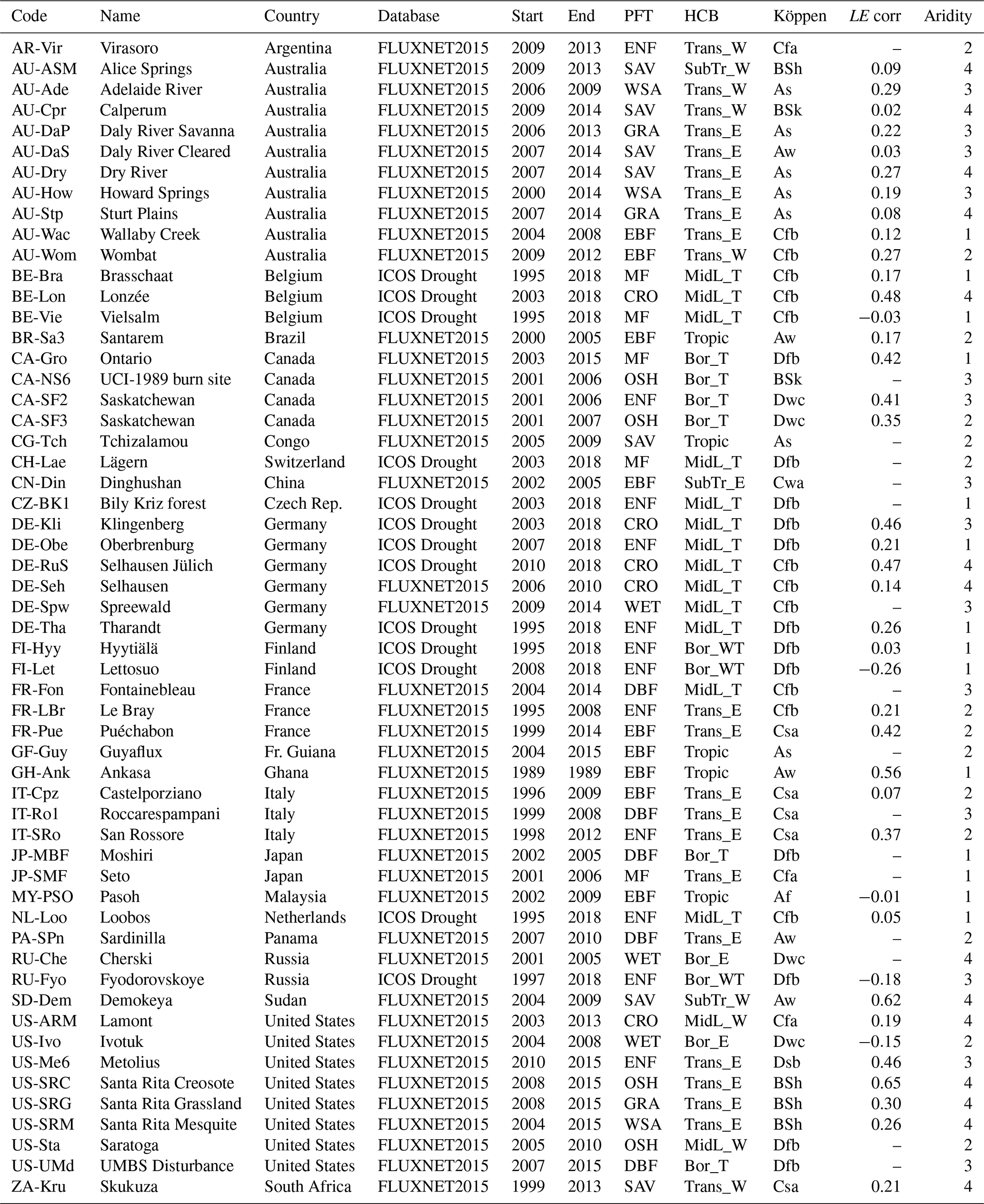
The performance of the models was evaluated at the field scale, using observations from flux towers. From the FLUXNET2015 dataset (Pastorello et al., 2020) and the ICOS “2018 drought initiative” dataset (Drought 2018 Team and ICOS Ecosystem Thematic Centre, 2019), sites were selected with adequate EC data quality (at least 1 year of carbon fluxes, dominated by observations with quality flag 1 or better), homogeneous land cover (within 1 km radius from the tower, assessed via Google Earth) and limited disturbance due to management. This resulted in the 56 sites listed in Table 2 and a total of 526 simulation years. A total of 33 of these sites are dominated by forest land cover, whereas 18 are dominated by herbaceous vegetation, and 5 are crop sites (the models are configured to run without management practices). The FLUXNET and ICOS data products had been pre-processed with the ONEFLUX processing pipeline (Pastorello et al., 2020). The test sites were classified per PFT (taken from the FLUXNET/ICOS IGBP metadata), dominant vegetation type (forest, herbaceous or crop) and hydro-climatic biome (HCB; Papagiannopoulou et al., 2018).

In addition to the classification based on land cover and meteorology, the sites were classified in “aridity classes”. In the LSMs, the root zone soil moisture modulates the stomatal conductance when it drops below field capacity (ISBA) or below 80 % of the difference between field capacity and wilting point (ORCHIDEE). As a proxy for aridity, the fraction of the simulation time that the simulated soil moisture in the topsoil (0–7 cm) drops below this threshold was used. It was found that this was significantly (Wilcoxon signed-rank test p<0.05) more frequent in ISBA (48 % of the time, median value of all sites) compared to ORCHIDEE (26 % of the time). Significant differences persisted deeper in the soil profile, until 70 cm depth. Using this metric, the sites were classified in four classes, equal in size, going from least (class 1) to most arid (class 4) (see Table 2). This classification was based on the ISBA simulations, but a similar classification was obtained with ORCHIDEE (despite the differences in absolute values). The vegetation at sites with aridity class 1 was mainly dominated by forest, whereas the aridity class 4 sites were mostly occupied by herbaceous vegetation. No evident relation with the hydro-climatic biomes was found.

Table 2 Selection of 56 FLUXNET/ICOS sites used in this study. Classification by PFT, HCB (boreal-/mid-latitude-/transitional-/subtropical-/tropical+energy-/water-/temperature-driven) and Köppen. LE corr: relative change in the mean LE flux after correction for energy balance closure (no value: correction not available). Aridity: aridity class, derived from ISBA simulations.

Not all sites are equipped with soil moisture sensors, nor is there a standardized set-up or post-processing for soil moisture in the datasets used for this study. Consequently, the validation of the simulated soil moisture and the sensitivity analysis was only performed for the sites with sensors. Furthermore, some sites were equipped with multiple sensors in the soil profile. Here, only the median score of the sensors was used in the statistics (i.e. one score per site). For the validation, all sensors up to 2 m depth were used, whereas only the sensors up to 0.5 m depth (i.e. the shallow root zone) were used in the sensitivity analysis (though the impact on the results was minimal).

2.3 Validation

The simulated H and LE were validated with the observed daily mean fluxes from flux towers. The non-closure of the energy balance is a well-known issue in the eddy covariance observations (Cui and Chui, 2019). The turbulent fluxes in the FLUXNET and ICOS datasets were corrected for this, under the assumption that the measured Bowen ratio was correct (Pastorello et al., 2020). Due to missing observations of the ground heat flux, this correction was not possible for all sites. The validation of H and LE was only performed for the sites where all fluxes were available. The mean correction of LE of each site is listed in Table 2.

Similarly, the simulated GPP was validated with the FLUXNET/ICOS GPP data. The net ecosystem exchange (NEE) observed at the flux tower was partitioned into its ecosystem respiration (RECO) and GPP components using the daytime fluxes and constant friction velocity (USTAR) threshold method (Pastorello et al., 2020). Only data with a quality flag indicating good quality (1) or better were used in this analysis. Though some authors have recommended correcting the carbon fluxes in a similar way as the turbulent fluxes, such a procedure was not included in the processing pipeline (Massman and Lee, 2002; Gao et al., 2019; see also Sect. 4).

An important key to the feedback mechanism between the surface fluxes is the LAI. The simulated LAI from ISBA-CC and ORCHIDEE was validated using the remote-sensing-based LAI from the European Copernicus Global Land Service (http://land.copernicus.eu/global/, last access: 15 July 2022). The LAI data product used here is derived from SPOT-VGT and PROBA-V satellite data; it has a spatial resolution of 1 km and a temporal resolution of 10 d (Camacho et al., 2013). The sites were selected to be fairly homogeneous within the footprint area, and the observed LAI is assumed to be representative of the direct surroundings of the eddy covariance stations.

The simulated soil moisture profiles of ISBA and ORCHIDEE and the ERA5 soil moisture (used in DiagMod) were validated where possible. To reduce biases caused by different soil physical properties of the soil profiles or differences in scale between models and observations, the observed and simulated volumetric soil moisture (θ) was converted to the effective saturation (S_e) as follows:

$$\begin{array}{}\text{(1)}& S_{\mathrm{e}}={\displaystyle \frac{\mathit{\theta }-{\mathit{\theta }}_{min}}{{\mathit{\theta }}_{max}-{\mathit{\theta }}_{min}}},\end{array}$$

where θ_min and θ_max were assumed to be the 5th and 95th percentile of the observed soil moisture at a site for the observations or the residual and saturated water content for the simulations.

For H, LE, GPP, LAI and S_e, the classical validation indices are calculated: mean error (ME), root mean square error (RMSE), Pearson correlation (r) and Nash–Sutcliffe model efficiency (NS). They were calculated as in Eqs. (2)–(5), in which y^* and y^o are the predicted and observed values, $\stackrel{\mathrm{‾}}{y}$ the mean of y, and n_o the number of observations:

$$\begin{array}{}\text{(2)}& {\displaystyle }\mathrm{ME}={\displaystyle \frac{{\sum }^{n_o}\left(y^{*}-y^o\right)}{n_o}}\text{(3)}& {\displaystyle }\mathrm{RMSE}=\sqrt{{\displaystyle \frac{{\sum }^{n_o}{\left(y^{*}-y^o\right)}^{\mathrm{2}}}{n_o}}}\text{(4)}& {\displaystyle }r={\displaystyle \frac{{\sum }^{n_o}(y^{*}-\stackrel{\mathrm{‾}}{y^{*}})(y^o-\stackrel{\mathrm{‾}}{y^o})}{\sqrt{{\sum }^{n_o}(y^{*}-\stackrel{\mathrm{‾}}{y^{*}}{)}^{\mathrm{2}}{\sum }^{n_o}(y^o-\stackrel{\mathrm{‾}}{y^o}{)}^{\mathrm{2}}}}}\text{(5)}& {\displaystyle }\mathrm{NS}=\mathrm{1}-{\displaystyle \frac{\sum (y^{*}-y^o{)}^{\mathrm{2}}}{\sum (y^o-\stackrel{\mathrm{‾}}{y^o}{)}^{\mathrm{2}}}}.\end{array}$$

Taylor diagrams were constructed using the Pearson correlation (r) and standard deviation (σ) of the observed and simulated variables. The validation was performed using the daily totals and averages.

Furthermore, the same analysis was also performed on the anomalies in the mean annual cycles to isolate the capability of the models to capture seasonal variability. The mean annual cycles were computed per site, across all its site years. The validation indices of the seasonal anomalies have the subscript ANOM, e.g. NS_ANOM.

Significant differences between the models were evaluated with the Wilcoxon signed-rank test (paired), and the significance of the PFT, HCB, aridity class and dominant land cover to classify the model performances was evaluated with the Kruskal–Wallis H test. Differences between classes were tested with the Mann–Whitney U test (non-paired).

2.4 Model dynamics

2.4.1 Phenology

The capability of the models to reproduce the timing of the seasonal cycle of LE, GPP and LAI was evaluated. The detection of the start, maximum and end of the seasonal cycle (SOS, MOS and EOS) was achieved by applying a smoothing operation (20 d rolling mean), followed by a threshold procedure (Maleki et al., 2020). In this threshold procedure, the minima and maxima were used to delineate the growing and senescent phase of the season. MOS was defined as the date when the maximum of the season is reached; SOS and EOS were defined as the date where the growing or senescent phase crosses the threshold value T. T was calculated for each growing or senescent phase as $T=P_{\mathrm{5}}+\mathrm{0.2}(P_{\mathrm{95}}-P_{\mathrm{5}})$, where P₅ and P₉₅ are the 5th and 95th percentile.

2.4.2 Partitioning

To compare the model dynamics, the simulated LE flux partitioning, water balance and water use efficiency (WUE) were evaluated as well. Direct observations of the LE flux partitioning were not available, but it is possible to extract the transpiration component from the total LE flux, using the underlying water use efficiency (uWUE) method (Zhou et al., 2016; Nelson et al., 2020). From the GPP and transpiration (Tr), the WUE was derived:

$$\begin{array}{}\text{(6)}& \mathrm{WUE}={\displaystyle \frac{\mathrm{GPP}}{\mathrm{Tr}}}.\end{array}$$

2.5 Evaluation of prognostic LAI and soil moisture

2.5.1 Sensitivity and error correlation

To assess the sensitivity of the fluxes to the state variables (S_e and LAI), the slope of the seasonal anomalies of the fluxes against the anomalies of the state variables was determined. This analysis was performed for the observations and the simulations and compared. Note that the linear slope was used here, though a linear response is not necessarily expected (e.g. the response to soil moisture anomalies depends on a wet/dry regime). The goal of this analysis was to investigate whether LSMs are capable of reproducing a similar relationship as found in the observations. Significant differences between the models were evaluated with the Wilcoxon signed-rank test.

To evaluate whether errors in the state variables result in errors in the surface fluxes (or vice versa), the Spearman rank correlation between both was calculated. Since Copernicus LAI was the reference LAI, this analysis was not possible for LAI in DiagMod.

2.5.2 Functional evaluation with DiagMod

The diagnostic model is a suitable vehicle to test the impact of the prognostic state variables from ISBA and ORCHIDEE on the surface fluxes. Given its architecture to easily ingest state variables, it can serve as an independent model platform to evaluate the quality of the soil moisture and LAI. DiagMod simulations were performed using soil moisture and/or LAI from ISBA and ORCHIDEE and compared to simulations with soil moisture from ERA5 and CGLS LAI (resulting in seven runs per site; see Table 4).

The fraction of absorbed photosynthetically active radiation (FAPAR) is an important variable in DiagMod to produce GPP, but it is no output of the prognostic models. In order to be consistent with the prognostic LAI, FAPAR was estimated using a simple Beer law with a general-purpose extinction coefficient value of 0.5 (Eq. 7; Monsi and Saeki, 2005).

$$\begin{array}{}\text{(7)}& \mathrm{FAPAR}=\mathrm{1}-\exp (-\mathrm{0.5}\mathrm{LAI})\end{array}$$

The soil moisture of the soil profiles in the prognostic models was integrated to match the four layers in DiagMod (0–7, 7–21, 21–72, 72–189 cm). Furthermore, the soil moisture was rescaled using the wilting point and field capacity parameters of the models.

Prior to the evaluation of the prognostic state, the reproducibility of the prognostic models by the DiagMod was tested. The detailed results are shown in the Supplement. It was found that the surface fluxes produced by DiagMod, forced by the same atmospheric conditions, soil moisture and LAI, were more closely correlated to those from ISBA compared to ORCHIDEE. Differences can be caused by different parametrization of the plant physiology, as well as the representation of processes (or lack thereof), such as rainfall interception, snow cover or canopy radiation transfer.

3 Results

3.1 Validation

3.1.1 Surface fluxes: LE and GPP

The bias (ME) and accuracy (RMSE) of the simulated LE and GPP are shown in Fig. 2, together with Taylor diagrams of the simulated fluxes and their seasonal anomalies. It was evident that the inter-site variability in the model performance is much larger than the inter-model variability. In terms of bias and accuracy, the differences between the models were relatively limited. All models suffered a substantial underestimation of LE, whereas the overall bias in GPP was relatively small. Significant differences (Wilcoxon p<0.05) were found in the bias of GPP between DiagMod (overestimation) and ISBA (underestimation), and the simulated LE was significantly more accurate in ISBA compared to ORCHIDEE.

Notably, no substantial bias was found in the simulated H of any model to compensate for the consistent bias in LE (results shown in the Supplement). In this study, the corrected fluxes from the FLUXNET/ICOS dataset were used as a reference. If the non-corrected fluxes were used instead, the bias in LE was reduced, but the simulated H was overestimated (not shown here). This points at the significant uncertainty associated with the observed fluxes from eddy covariance measurements. The estimated observation uncertainty in the turbulent fluxes (associated with random measurement errors and energy balance correction) had the same order of magnitude as the model errors.

The Taylor diagrams in Fig. 2 show that the average variability in the simulated LE and GPP was in fair agreement with the observations. After removal of the mean seasonal cycle, the performance of the models decreased (r_ANOM, NS_ANOM), but the mean variability in the anomalies is reasonably accurate. In terms of r and r_ANOM of LE and GPP, ORCHIDEE was significantly outperformed by ISBA and DiagMod (Wilcoxon p<0.05). No significant differences were found between ISBA and DiagMod.

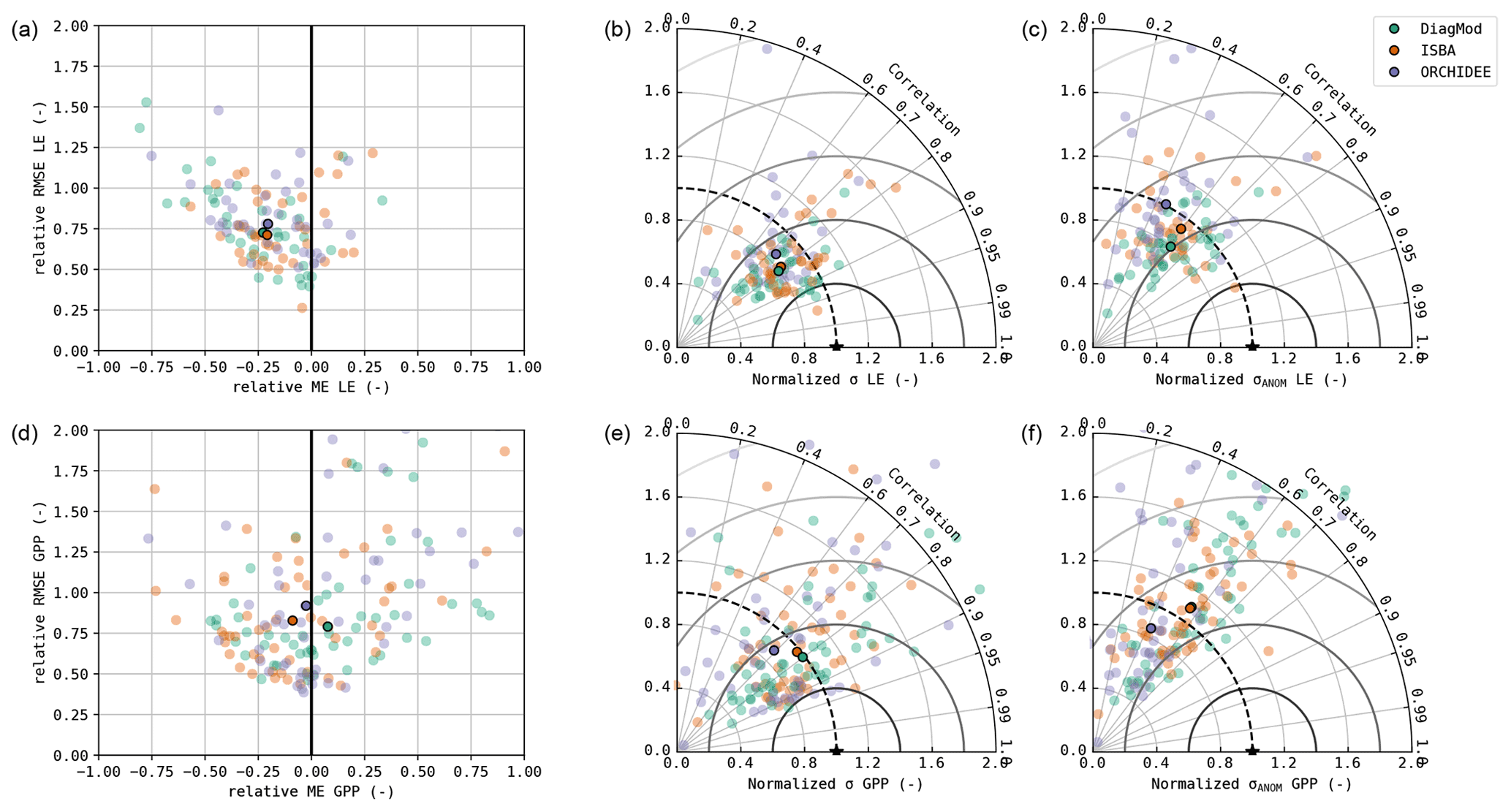
Figure 2 Accuracy plot (a, d), Taylor diagram (b, e) and Taylor diagram of the seasonal anomalies (c, f) of the simulated daily mean LE (a–c) and GPP (d–f). The median performance is shown with the opaque markers.

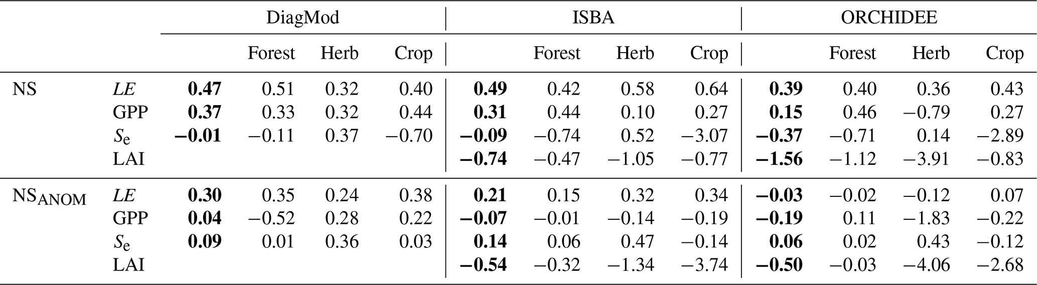
The impact of the land cover type of the test site on the model performance is illustrated in Fig. 3. Here, the test sites are classified by the dominant vegetation type. The NS and NS_ANOM of the simulated LE were not significantly impacted in any of the models, whereas a significant influence (Kruskal p<0.05) was found on the quality of the simulated GPP in DiagMod and ORCHIDEE. The NS and NS_ANOM of the simulated GPP in ORCHIDEE were significantly better (Mann–Whitney U p<0.05) for forest sites compared to sites that were dominated by herbaceous vegetation. Inversely, the simulation of the seasonal GPP anomalies in DiagMod were significantly better at herbaceous test sites (Mann–Whitney U p<0.05). No significant impact was found in the ISBA simulations. Notably, the differences between the models were most pronounced at the herbaceous sites (see also Table 3). Yet, despite its poorer performance at the herbaceous sites, ORCHIDEE simulated GPP at forest sites most accurately compared to the other models.

Table 3 Nash–Sutcliffe model efficiency coefficient of LE, GPP, S_e and LAI and their seasonal anomalies. Median scores given for all sites and grouped per dominant land cover type. The scores for the DiagMod S_e are computed using the ERA5 S_e. Overall median scores are given in bold font.

Figure 3 NS and NS_ANOM of the simulated daily LE and GPP, grouped per land cover type.

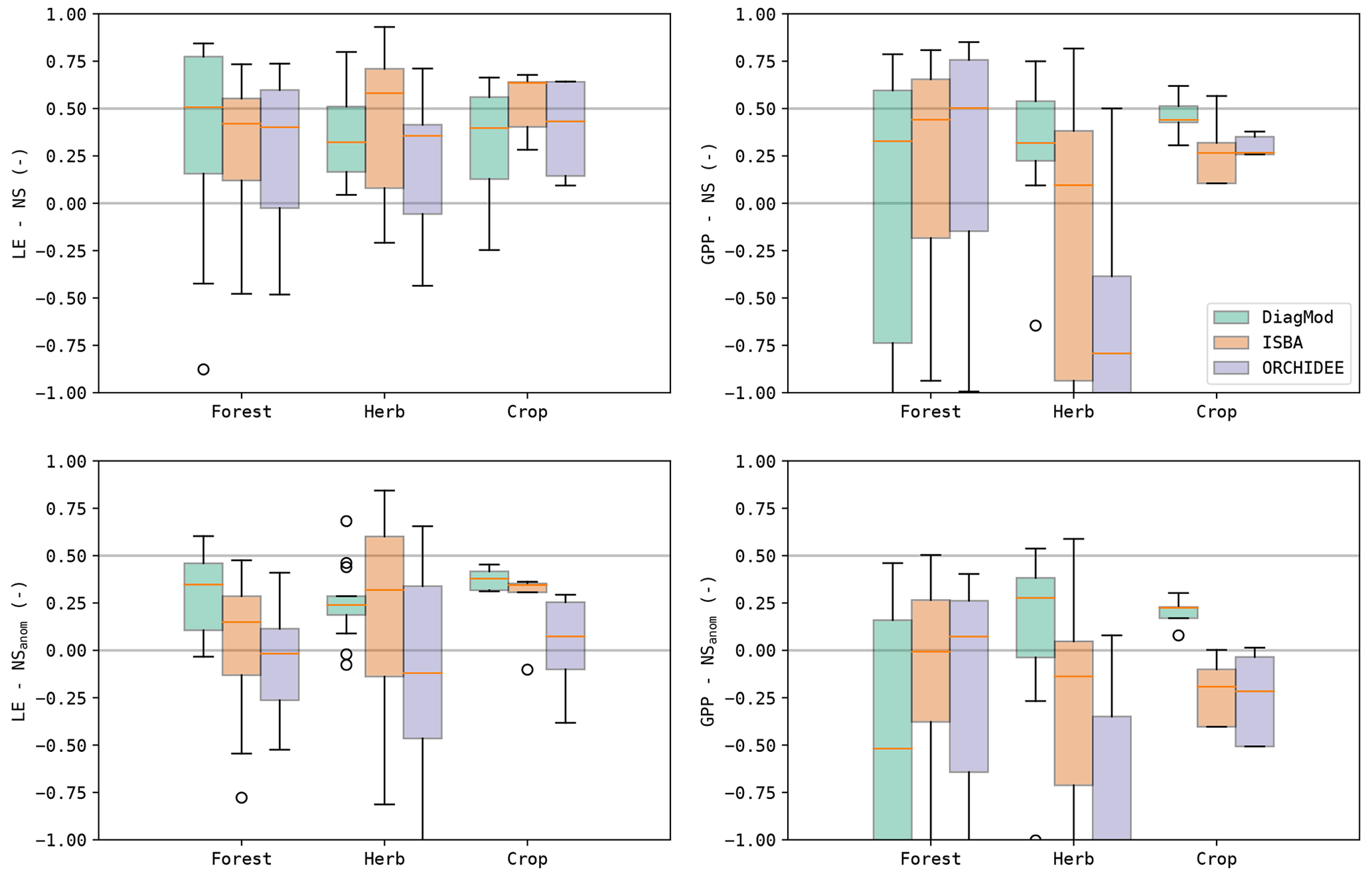
Similar results were found with the other validation indices. A more detailed breakdown of the results per PFT and HCB is given in the Supplement. A significant impact of PFT and HCB on the NS of the simulated GPP (Kruskal p<0.05) was found in all models. This was contrasted by LE, where a significant impact of HCB (Kruskal p<0.05) was found only for ORCHIDEE.

3.1.2 State variables: soil moisture and LAI

The validation results of S_e and LAI are shown in Fig. 4. The soil moisture from ERA5 (used in DiagMod) tended to be overestimated compared to in situ observations, whereas an overall negative bias was found in ISBA and ORCHIDEE. The simulated variability in soil moisture was too low in all models, in particular for ORCHIDEE. Notably, ERA5 outperformed ISBA (p>0.05) and ORCHIDEE (p<0.05) in terms of accuracy, despite their use of in situ meteorological forcings (e.g. precipitation). ORCHIDEE performed significantly worse than the other two models for all validation metrics (Wilcoxon p<0.05). The highest correlation in the anomalies was simulated by ISBA.

Compared to the surface fluxes, the accuracy of the simulated soil moisture was substantially lower. The validation scores of S_e are given in Table 3, separated per dominant land cover type. In all models, the simulated S_e was significantly better for herbaceous sites compared to forest sites. The herbaceous sites are generally found in a water-driven dryland climate, with strong precipitation-driven anomalies.

Similarly, the prognostic LAI was also of poorer quality than the simulated surface fluxes. ISBA had a significantly better ME and RMSE than ORCHIDEE, but both models overestimated LAI and strongly underestimated its variability. In particular, the variability in LAI in the evergreen needleleaf forests was strongly underestimated in both models, as well as the variability in LAI in evergreen broadleaf forests in ORCHIDEE. Furthermore, both models obtained only a poor correlation and achieved a very poor correlation of the seasonal anomalies. In both models, the simulated LAI for forest sites was better than for the herbaceous sites, though not significantly (p>0.05). The simulated anomalies were modelled significantly better (p<0.05) at forest sites than herbaceous sites (Table 3).

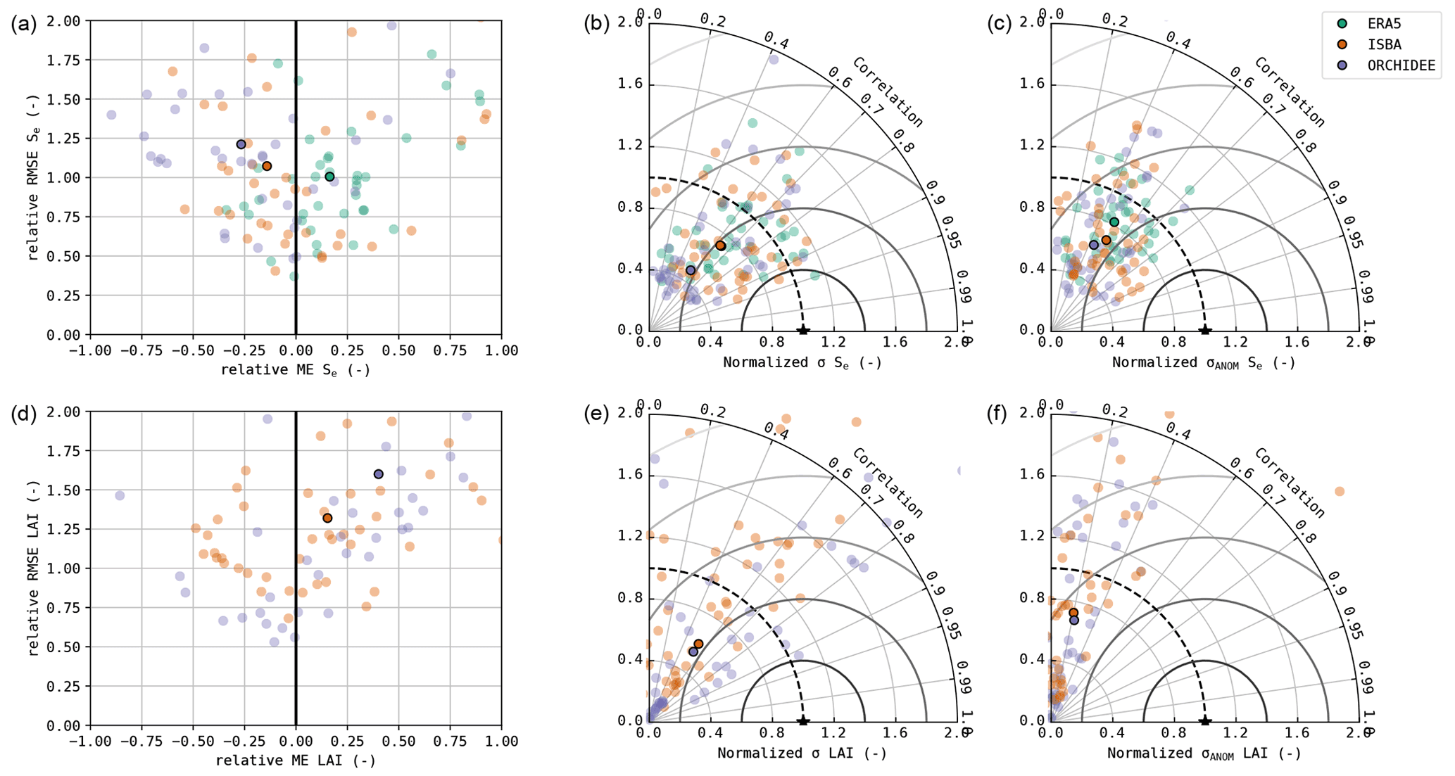
Figure 4 Accuracy plot (a, d), Taylor diagram (b, e) and Taylor diagram of the seasonal anomalies (c, f) of S_e (a–c) and LAI (d–f). The median performance is shown with the opaque markers.

3.2 Model dynamics

3.2.1 Phenology

The timing of the start, maximum and end of the seasonal cycle was validated for LE, GPP and LAI. Figure 5 shows the boxplots of the mean errors at all sites. In all models, the bias and accuracy of the seasonality of LE and GPP were comparable, whereas the leaf phenology (i.e. LAI) was poorer. The simulated phenology of LAI was delayed substantially, in particular in ISBA. This bias was most pronounced by the MOS, and to a lesser extent in EOS.

ISBA performed significantly worse than ORCHIDEE (Wilcoxon p<0.05) for ME of MOS GPP and MOS LAI and RMSE of MOS LAI. The prognostic LAI in both models tended to peak towards the end of the growing season, whereas the maximum LAI was reached in the beginning of the season according to the observations. This is illustrated in Fig. 6, where the mean annual LE, GPP and LAI cycles of ENF and DBF sites are shown. The delayed GPP phenology in ISBA is a feedback effect of the delayed prognostic LAI. However, the effect is dampened since GPP is largely driven by atmospheric forcings as well.

At forest sites, EOS of LAI tended to be simulated with the highest accuracy. The phenology of herbaceous sites had a higher variability (median standard deviation of EOS LAI at forest sites was 7.7 d compared to 20.6 d at herbaceous sites), which turned out to be challenging to capture for ISBA and ORCHIDEE. An example is shown for the savanna sites in Fig. 7. DiagMod relied on the remote-sensing-based LAI and was significantly more accurate than the prognostic models in capturing EOS of GPP (Wilcoxon p<0.05).

As the models were configured to run without dedicated management practices for the crop sites, EOS was estimated too late due to the harvest practice (Fig. 7). Even in DiagMod, EOS of GPP was delayed.

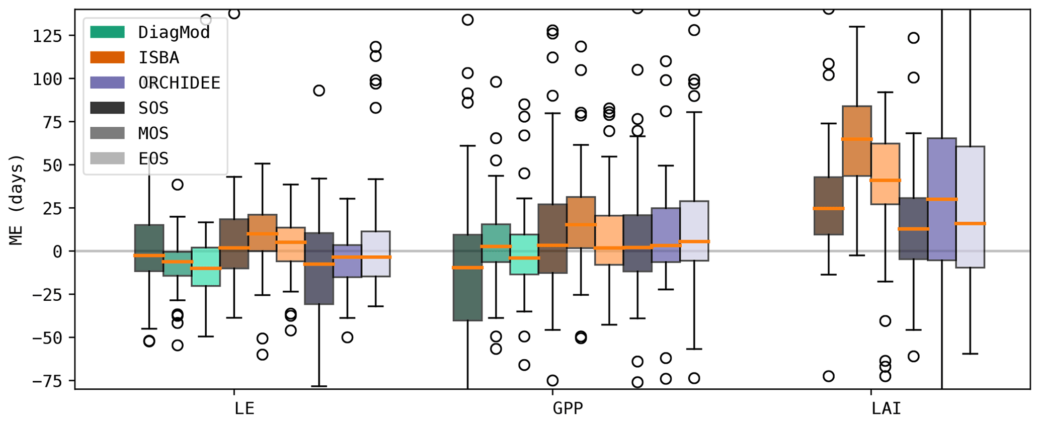
Figure 5 Mean error in the timing of the simulated seasonal cycle (start, max and end of season) for LE, GPP and LAI.

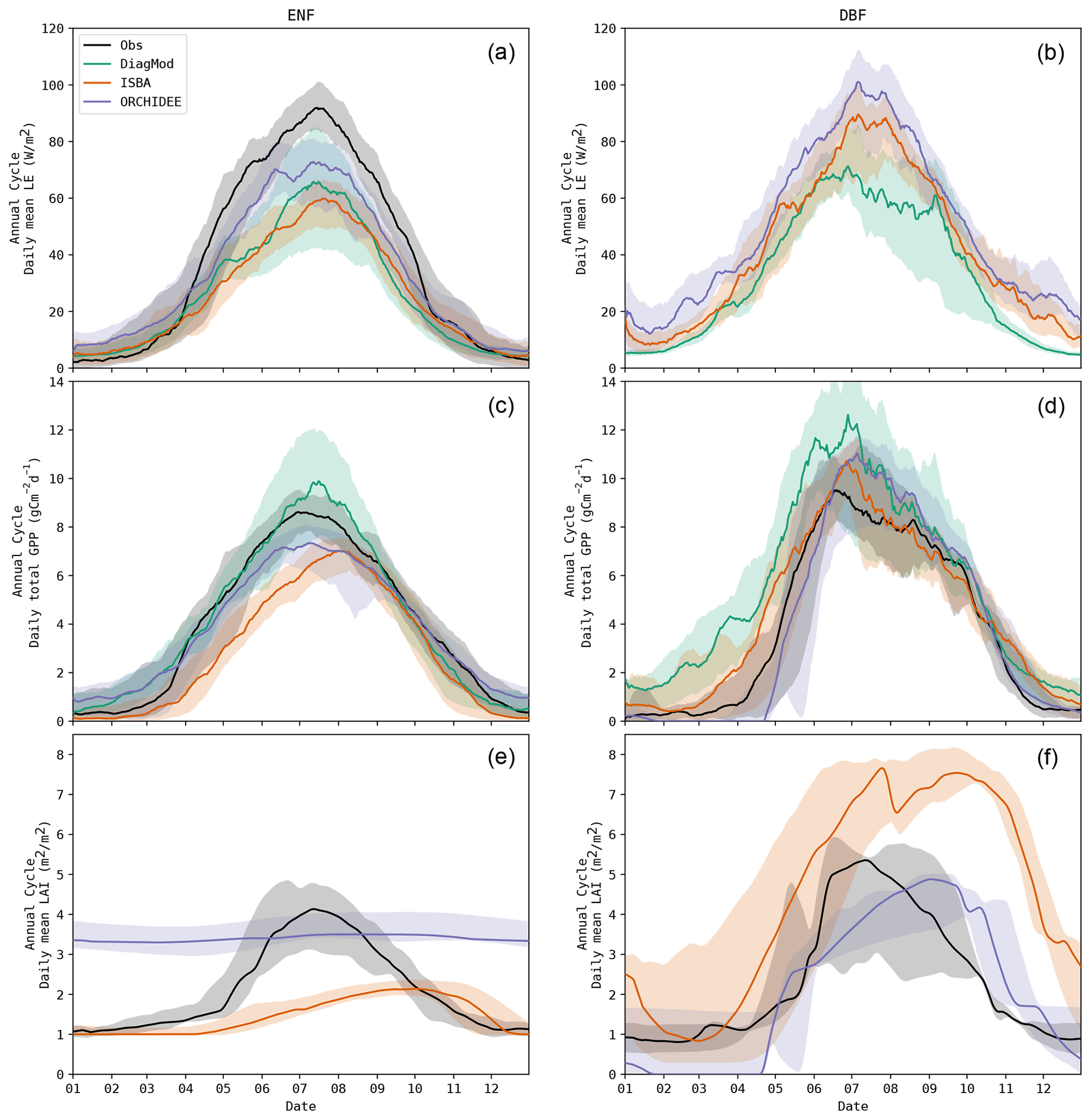
Figure 6 Mean annual cycle for LE, GPP and LAI in all evergreen needleleaf forest (a, c, e) and deciduous broadleaf forest (b, d, f) sites, observed and simulated. Note: corrected LE observations were missing at all DBF sites.

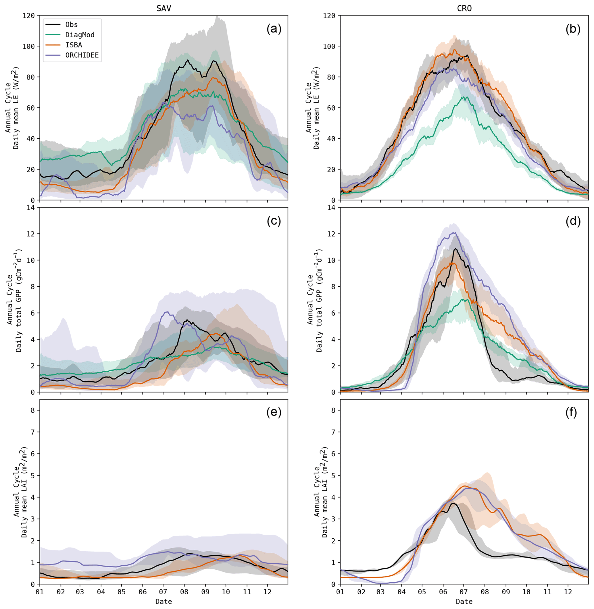
Figure 7 Mean annual cycle for LE, GPP and LAI at all savanna (a, c, e) and crop (b, d, f) sites, observed and simulated.

3.2.2 Water balance, WUE and LE partitioning

The water balance partitioning in ISBA and ORCHIDEE is shown in Fig. 8. In both models, the evapotranspiration fraction across PFTs was similar, but substantial differences were found in the drainage and runoff in both models. Whereas nearly no water was lost through runoff in the ISBA simulations, a substantial amount of runoff was simulated with ORCHIDEE. On the other hand, the drainage in ISBA was consistently larger than in ORCHIDEE. DiagMod does not compute a water balance, so it could not be included in this comparison.

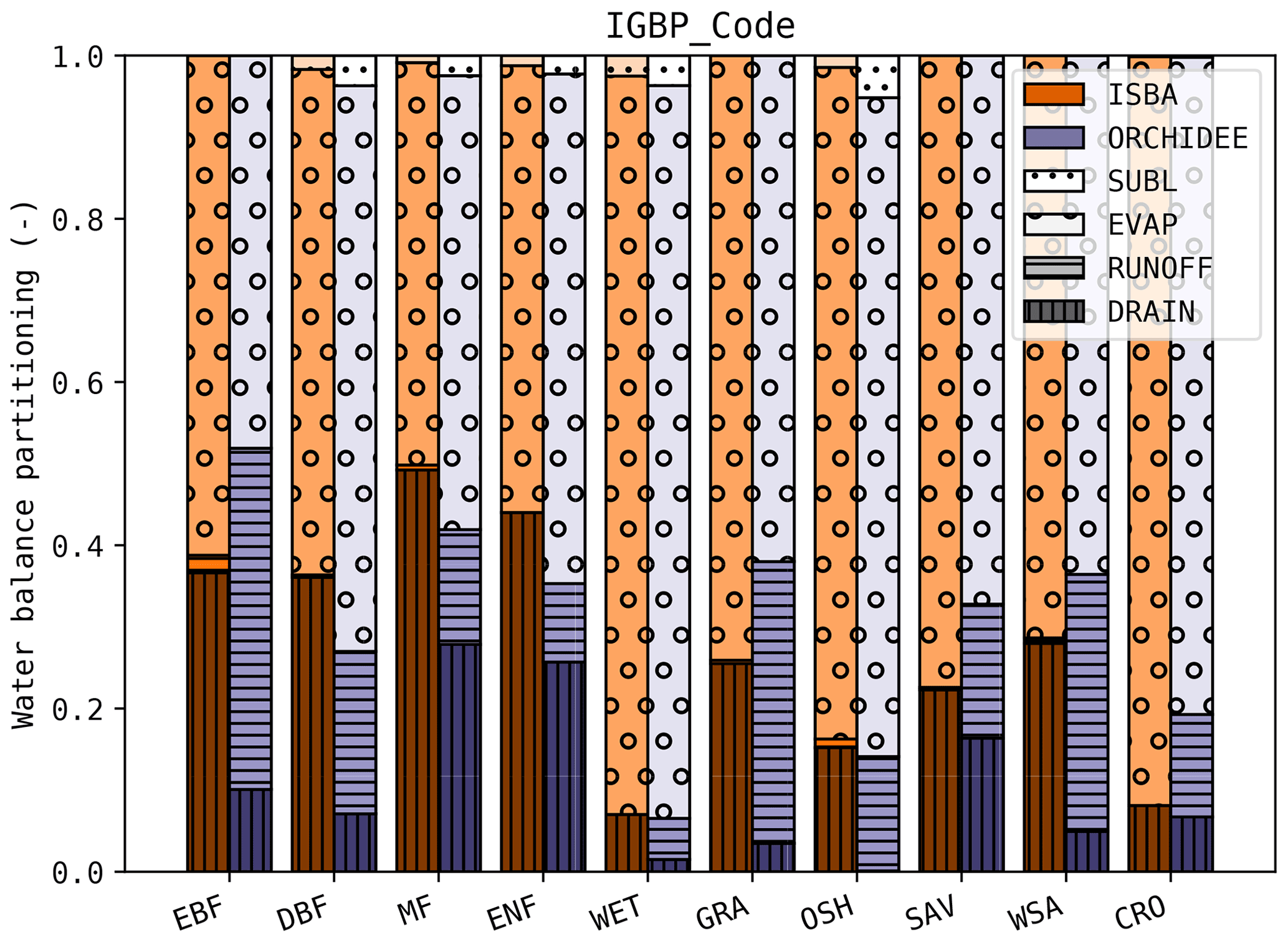
Figure 8 Average water balance partitioning (deep drainage, runoff, evapotranspiration and sublimation) per PFT class in ISBA and ORCHIDEE.

Both models agreed that the largest fraction of LE is through transpiration of the vegetation (Fig. 9). Aside from a few exceptions, T $/$ ET in ORCHIDEE was larger than in ISBA. The median T $/$ ET in ISBA (0.53) is lower than in ORCHIDEE (0.68) and is closer to the values derived from the tower observations with the uWUE method (0.54). However, measurements by Lian et al. (2018) indicate that this is an underestimation and suggest 0.62±0.06 as a global estimate.

Figure 9 Average LE partitioning per PFT class in ISBA and ORCHIDEE. LETR: transpiration; LER: intercept evaporation; LEG: soil evaporation; LEI: ice/snow evaporation; other: including evaporation from flooded surfaces.

When the observed average water use efficiency is plotted versus the average LE flux, a pattern emerges in which the sites are grouped per PFT (Fig. 10). A similar pattern was found in the ISBA simulations, but not in the ORCHIDEE simulations. The range in WUE across the test sites was much smaller in ORCHIDEE than in the observations.

Figure 10 Median water use efficiency and LE in observations and simulations. Sites classified per PFT.

The difference in water use efficiency can be attributed to differences in the modelled plant physiology or the amount of drought stress experienced by the vegetation. As mentioned above, the root zone soil moisture dropped significantly more frequently below field capacity in ISBA compared to ORCHIDEE.

3.3 Evaluation of prognostic LAI and soil moisture

3.3.1 Sensitivity and error correlation

The sensitivity of the surface fluxes to soil moisture and LAI was quantified with a simple linear regression between their anomalies. The slope of these regressions indicates the strength of the response to the state variables.

It was found that the sensitivity of the fluxes to the soil moisture was strongly dependent on the land cover type, in both the observations and the models (Fig. 11). A stronger response was found at the herbaceous sites compared to the forest sites. ISBA and ORCHIDEE have too high a sensitivity to soil moisture, whereas the response in the diagnostic model was closer to that in the observations. In Fig. 12, the same data are plotted but classified per aridity class. This illustrates the oversensitivity of ISBA and ORCHIDEE to drought stress. Despite their differences in implementation and parametrization, a striking similarity in their sensitivity to drought was found, for both LE and GPP. The observations did not show an increase in sensitivity of GPP to S_e at dryer sites.

At the forest sites, the response of GPP to S_e anomalies is counterintuitively negative. This might indicate that soil moisture anomalies at forest sites were more dominated by wet anomalies, associated with rainfall events. These events coincide with a reduction in solar radiation, hence resulting in a negative GPP response. At herbaceous sites soils were generally drier, so the positive impact of the reduced drought stress after the rainfall event was more dominant, resulting in a positive response. This behaviour was mimicked well in the models.

The sensitivity of LE and GPP to LAI was generally higher at the herbaceous sites. Here, the models tended to underestimate the sensitivity to LAI. At the forest sites, the sensitivity was lower according to the observations. The modelled sensitivity of LE to LAI was reasonably accurate, whereas the sensitivity of GPP to LAI was too strong.

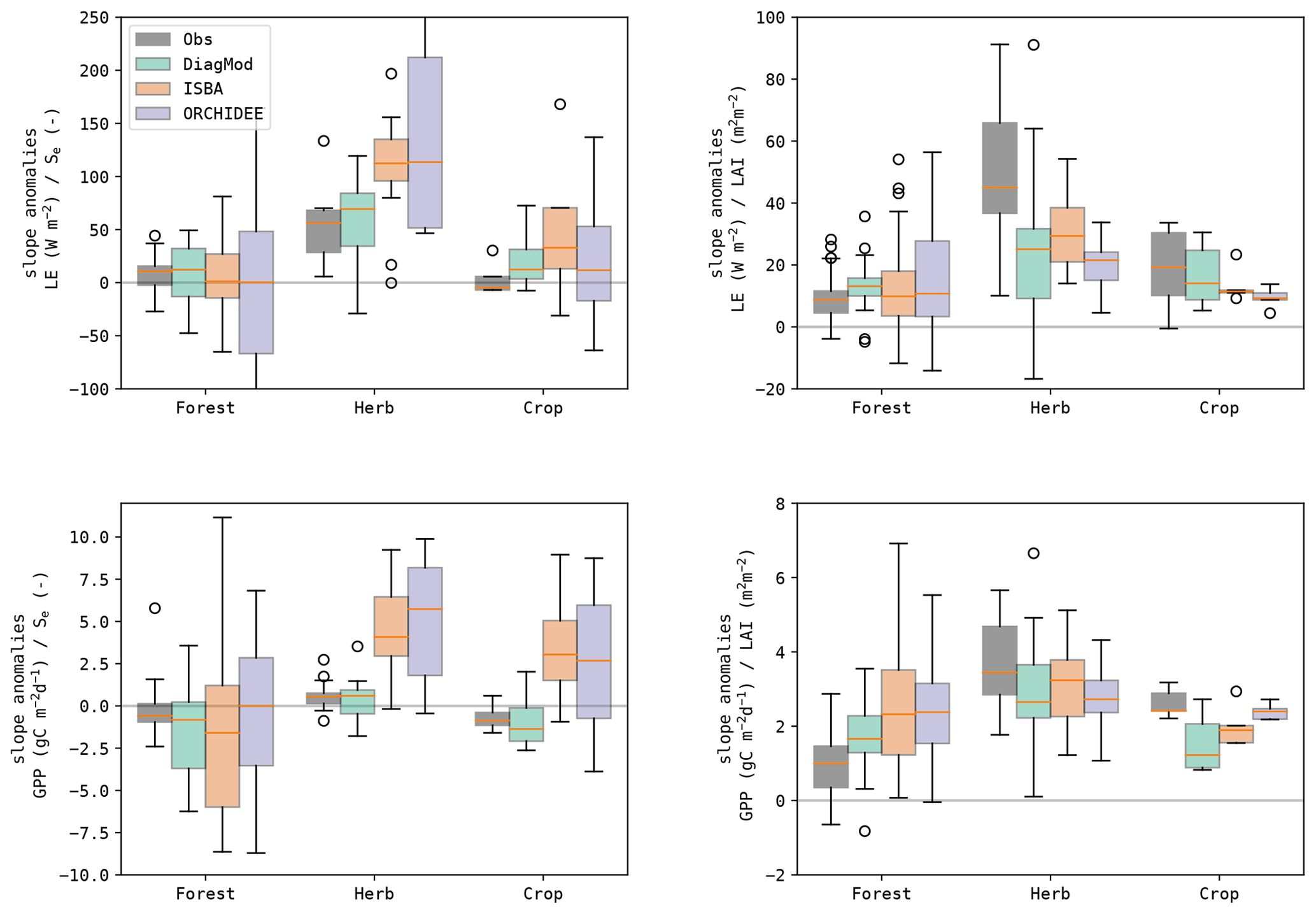
Figure 11 Boxplots of the slope of the linear regression between the anomalies in the state variables (S_e and LAI) and the fluxes (LE and GPP) at the test sites, grouped per dominant land cover.

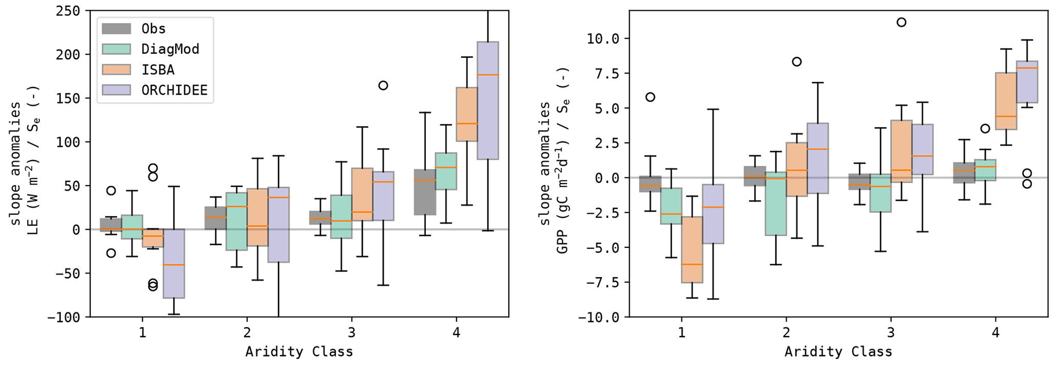
Figure 12 Boxplots of the slope of the linear regression between the anomalies in the state variables (S_e and LAI) and the fluxes (LE and GPP) at the test sites, grouped per aridity class (1: least frequent drought stress; 4: most frequent drought stress).

To evaluate the impact of the quality of S_e and LAI on the simulated surface fluxes, the Spearman correlation of the errors in the state variables and the fluxes was calculated (Fig. 13). It was found in both ISBA and ORCHIDEE that LAI had a stronger error correlation to LE and GPP compared to S_e. Grouped per dominant land cover type (Fig. 14), both models agree that the error correlation between LAI and GPP was higher at the herbaceous sites compared to the forest sites. Notably, this was not the case for LAI–LE.

Furthermore, the errors in LE were most strongly correlated to those in S_e for all models. The highest error correlation was found in DiagMod, where this was most pronounced for the herbaceous sites. At these sites, the S_e–GPP error correlation was also the strongest for DiagMod, whereas no strong S_e–GPP error correlation was found in the other models.

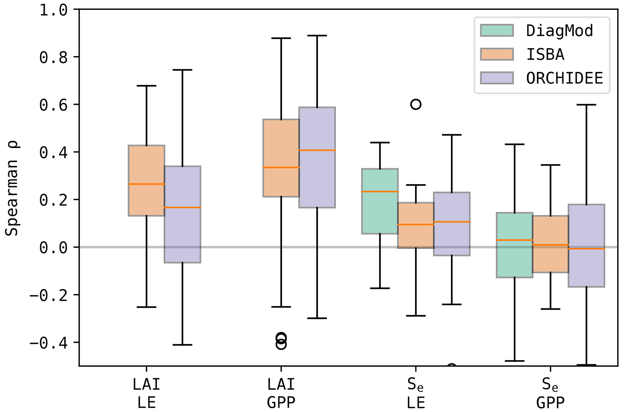
Figure 13 Boxplots of the Spearman correlation between the errors in the state variables (S_e and LAI) and the fluxes (LE and GPP) at all test sites.

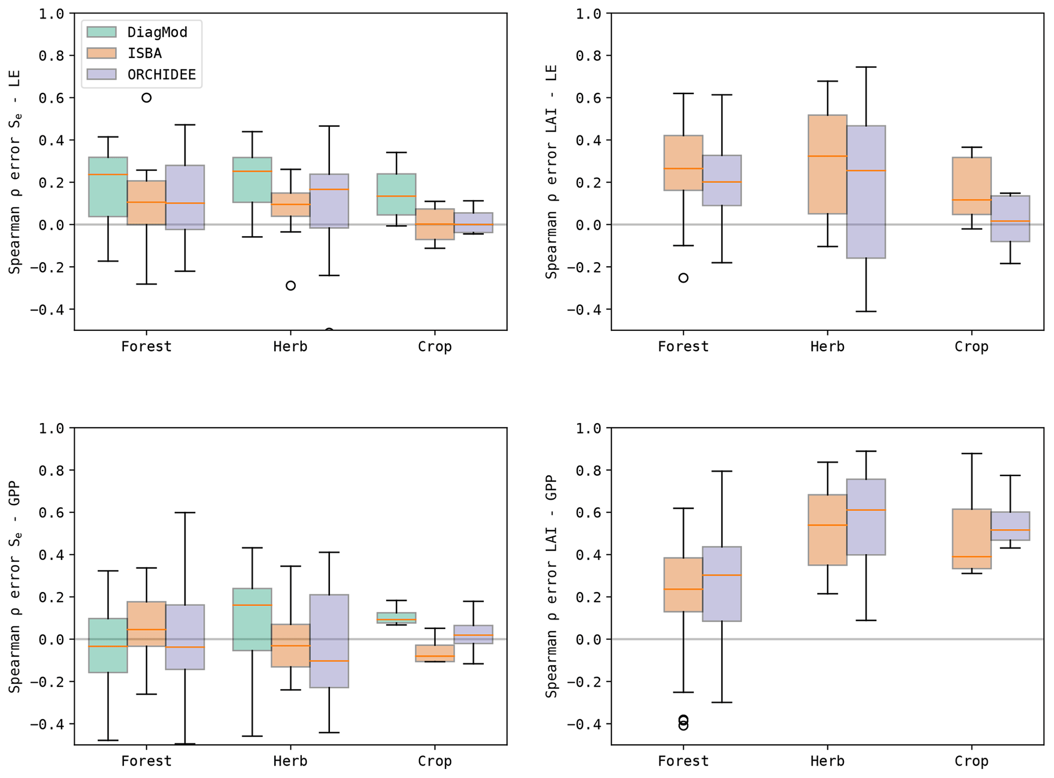
Figure 14 Boxplots of the Spearman correlation between the errors in the state variables (S_e and LAI) and the fluxes (LE and GPP) at the test sites, grouped per dominant land cover.

3.3.2 Functional evaluation with DiagMod

The simulated LE and GPP from the DiagMod runs with soil moisture and/or LAI from the prognostic models were validated with tower observations. The resulting NS is shown in Table 4 and Fig. 15. Similar tendencies were found in RMSE, Pearson r and validation of the seasonal anomalies (not shown here). The DiagMod run with CGLS LAI and ERA5 soil moisture serves as a reference to evaluate the prognostic state variables.

Soil moisture had a stronger impact on LE compared to LAI. A significant (Wilcoxon p<0.05) reduction in NS was found when using soil moisture from ORCHIDEE. This effect is most pronounced at the herbaceous (more water-limited) sites. This is in contrast with the runs using soil moisture from ISBA, which seemed to improve the simulated LE at herbaceous sites (though not significantly). Similar but smaller effects were found at the forest (less water-limited) sites. On the other hand, the opposite was found for the crop sites (n=4) where simulations with soil moisture from ISBA reduced the NS of the simulated LE significantly.

Despite strong differences in LAI, no significant impact was found on LE (with the exception of crop sites with ISBA LAI). A stronger sensitivity to LAI was found in the DiagMod simulations of GPP. A significant reduction in NS was found in all DiagMod runs, but most explicitly in the runs using the prognostic LAI. As in the simulations of LE, this was most pronounced for the herbaceous sites. The use of LAI from ISBA and ORCHIDEE strongly degraded the simulated GPP at these sites, whereas it was unaffected by injecting the prognostic soil moisture.

Overall these results are in line with the error correlations in Fig. 13. The higher error correlation of LAI to LE and GPP compared to the error correlations of soil moisture was confirmed. Additionally, the stronger impact of prognostic LAI on errors in GPP and of soil moisture on LE was found in both analyses.

Table 4 Median Nash–Sutcliffe model efficiency index of the DiagMod runs (functional evaluation of the prognostic LAI and soil moisture). Results presented for all sites and classified per dominant land cover. Significant differences (Wilcoxon p<0.05) with reference DiagMod runs are marked. Overall median scores are given in bold font.

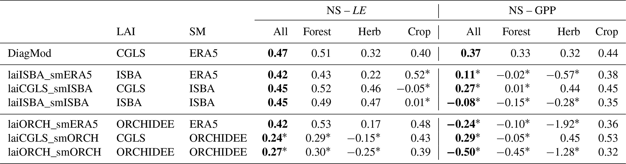
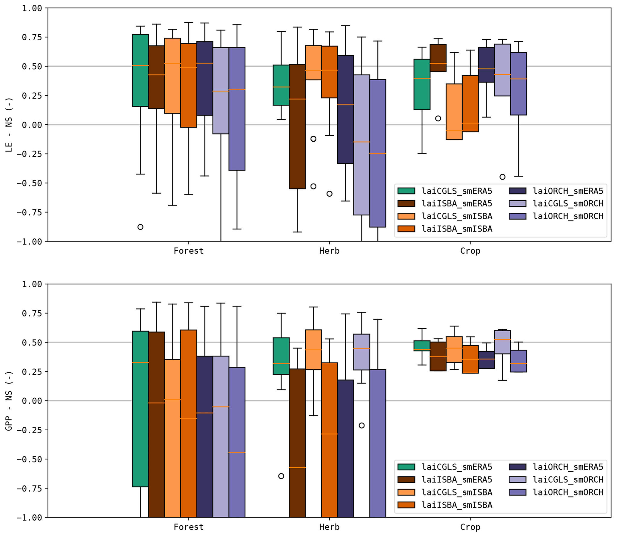
Figure 15 Nash–Sutcliffe model efficiency index of the DiagMod runs for the functional evaluation.

4 Discussion

4.1 Model performance

The validation metrics of the three models were generally in agreement with previously performed local-scale evaluations. Similar simulations with the diagnostic model were done in the validation reports of both the LSA SAF evapotranspiration and surface flux products (Ghilain et al., 2018) on one hand and the LSA SAF GPP product (Martínez et al., 2020) on the other hand. The accuracy and Pearson correlation obtained here were better than the ones previously reported. This can be attributed to the use of local forcings in this study, which are not used in the LSA SAF products. The weaker performance of the algorithm for the sensible heat flux was also identified by Ghilain et al. (2018).

The GPP product is a recent addition to the ensemble of LSA SAF MSG products. It was demonstrated to outperform similar products which also rely on the Monteith light-use efficiency method (Martínez et al., 2020). Here, it was found to perform consistently well for forest and herbaceous sites and achieve a comparable model performance to ISBA.

In previous intercomparison studies at the local scale (Balzarolo et al., 2014) or global scale (Friedlingstein et al., 2021), GPP was simulated more accurately with ORCHIDEE than with ISBA, but this was not confirmed here. Since these studies, substantial improvements have been made to ISBA: introduction of the MEB scheme, parametrization update, diffuse multilayer soil scheme, etc. (Boone et al., 2017; Delire et al., 2020). The introduction of the MEB scheme for forests on the energy fluxes was evaluated in-depth by Napoly et al. (2017) at the local scale (though prognostic LAI was not included in that study). Substantial improvements to G and H were reported, thanks to the addition of an insulating litter layer. The introduction of the MEB scheme improved the mechanistic representation of the canopy, and issues due to a shared roughness length of the vegetation and bare soil in the composite scheme were circumvented. Our findings agree with that outcome, but the bias we found for LE is not in agreement with previous findings.

4.1.1 Observation uncertainties

With the emergence of freely available data from eddy covariance networks, the use of local datasets is an increasingly standardized approach to evaluate the performance of land surface models (Balzarolo et al., 2014; Napoly et al., 2017; Williams et al., 2020; Chen et al., 2018; Joetzjer et al., 2015). However, the eddy covariance observations notoriously suffer from substantial biases and non-closure of the energy balance (Foken, 2008; Mauder et al., 2020). The non-closure of the energy balance is attributed to (1) large advective fluxes caused by surface heterogeneities; (2) systematic measurement errors due to mismatch in observation footprint or inadequate sample rate; or (3) thermal processes, such as heat storage or vegetation metabolism (Mauder et al., 2020; Chu et al., 2021; Liu et al., 2021). The test sites in this study were selected to have a relatively homogeneous land cover. Regardless, the resulting uncertainty in the observations was of the same order of magnitude as the model errors. The turbulent fluxes are typically underestimated, as is the GPP (Massman and Lee, 2002; Gao et al., 2019). Note that GPP is not corrected for this possible bias in the ONEFLUX processing pipeline (Pastorello et al., 2020). Furthermore, some studies have indicated that the eddy covariance observations are closer to lysimeter data if the energy balance is closed by correcting LE only (Wohlfahrt et al., 2010). Considering this, the negative bias of the simulated LE (and GPP) in this study could be even underestimated. Conversely, others suggest that most or all of the deficit might be related to H (Ingwersen et al., 2011) or found a good match with independent reference data without LE correction (Graf et al., 2014). Validation results of the turbulent fluxes without energy balance closure correction are given in the Supplement.

4.1.2 Forest vs. herbaceous

Generally, the differences between the accuracy of the simulated surface fluxes was most distinct at the sites dominated by herbaceous vegetation (excluding crop sites). These sites have the most pronounced inter-annual variability, and seasonal anomalies are strongly driven by precipitation events (Weber et al., 2009). This can be largely attributed to their natural occurrence in dryer climates and shallower root system compared to forests. The seasonal cycle of LAI at the herbaceous sites and its variability were simulated poorly with the prognostic models. The error correlation analysis indicated that these errors were strongly related to errors in the surface fluxes.

At the crop sites, management practices were missing in the prognostic models. In the mean annual cycle of LAI (Fig. 7), it is evident that no harvest occurs. Despite this, the simulations of LE were not significantly less accurate compared to other land cover types. After harvest, LE consists largely of bare soil evaporation. Though vegetation was still present in the models, the bulk LE was still reasonably accurate. More evident degradation of the results was found in GPP after harvest, which was overestimated. Even in the diagnostic model, where management practices were incorporated implicitly in the forcing variables, GPP was overestimated. Notably, despite the missing management practices in the prognostic models, the quality of the simulated LE and GPP (and their anomalies) was not significantly different from that at natural herbaceous sites.

Still, the diagnostic model performed consistently well for all types of land cover, contrary to the prognostic models. Only the seasonal variability in GPP at forest sites was simulated less accurately than with the prognostic models. Whereas the remote-sensing-based observations adequately captured this variability for the herbaceous and crop sites, they seemed to fall short for the forest sites.

4.2 Interactions

LAI and soil moisture are two key variables in the interaction between water, energy and vegetation. Though our understanding of the involved processes at the leaf-level scale is advanced, it remains challenging to scale these relations to the canopy level. This was illustrated by erroneous sensitivity of the models to LAI and soil moisture. As in previous studies, the sensitivity of LE and GPP to soil moisture was generally overestimated (Piao et al., 2013; Huang et al., 2016) in ISBA and ORCHIDEE, whereas the diagnostic model represented the observed sensitivity relatively well.

The interplay between LE and LAI was analysed in detail by Forzieri et al. (2018, 2020). The estimated global sensitivity of LE to LAI (3.66±0.45 W m⁻² (m² m⁻²)⁻¹, according to Forzieri et al., 2020) is lower than the one reported here, but the applied methodology was not the same. Contrary to our study, anomalies due to climatic drivers (i.e. precipitation, temperature, etc.) were factored out, resulting in a different response. The oversensitivity of LE to LAI in ORCHIDEE was also not confirmed in our study. Still, in accordance with these studies, a stronger response between LE and LAI was found for herbaceous/soil-moisture-supply-driven sites compared to forest/demand-driven sites.

Despite the differences in their architecture and parametrization, ISBA and ORCHIDEE demonstrated similar behaviour in the interaction between water, energy and vegetation. Comparable sensitivities and error correlations were found in both models, indicating that they share common weaknesses in their implementation.

4.2.1 LAI

The errors in the surface fluxes were strongly correlated to errors in LAI for both prognostic models, even though their sensitivity to LAI reflects the observed sensitivity reasonably well (compared to the sensitivity to soil moisture). This seemed to indicate that the source of the errors in the fluxes lies in the feedback mechanism between GPP and LAI (i.e. biomass allocation and phenology), rather than in the forward link between GPP and LAI (i.e. photosynthesis and leaf to canopy upscaling).

The prognostic simulation of LAI in ISBA was introduced by Gibelin et al. (2006) and uses a fairly simple scheme. The latest update was the revision of plant trait parameters according to the TRY database (Kattge et al., 2011; Delire et al., 2020). It has frequently been reported that the seasonal cycle of the simulated LAI in ISBA is delayed by a month or more (Lafont et al., 2012; Gibelin et al., 2008; Joetzjer et al., 2015). Delire et al. (2020) attributes this to the leaf longevity parameter, and Szczypta et al. (2014) mention the vegetation undergrowth dynamics as a possible cause for the mismatch between remote-sensing-based LAI and the prognostic LAI in LSMs. However, the issue seems to be related to the architecture of the biomass allocation scheme as well. The assimilated carbon is attributed to the leaf biomass pool first, from where it trickles down to the other pools. No carbon reserve dynamics are implemented. The consequence is that the simulated LAI in ISBA starts slow during spring, as GPP is underestimated due to a low LAI. It continues to build up LAI until late in the second half of the season, when photosynthetic conditions become suboptimal, and leaf senescence is triggered. In contrast, the observed seasonal LAI cycles reach a maximum in the first half of the growing season.

The functional evaluation with the diagnostic model demonstrated that a fairly simple model is capable of simulating the surface fluxes accurately, given accurate observations of LAI. The prognostic LAI generally degraded the results compared to simulations with remotely sensed LAI. Data assimilation experiments have demonstrated the potential of remotely sensed LAI to improve the surface fluxes (Albergel et al., 2017). Improvements to prognostic LAI schemes are required to increase the skill of the LSMs to simulate surface fluxes.

In that context, processes from ORCHIDEE and other LSMs could be adopted to improve the fairly simple biomass allocation scheme in ISBA. The importance of non-structural carbohydrates to capture the leaf phenology in LSMs is well known, though rarely implemented (Asaadi et al., 2018). Fatichi et al. (2019) indicates that a full-grown canopy of a deciduous broadleaf forest contains approximately 30 % of the total yearly assimilated carbon, yet it is grown in 1 month ($\mathrm{1}/\mathrm{5}$–$\mathrm{1}/\mathrm{6}$ of the growing season). This rough simplification illustrates that reserve dynamics are essential to simulate the seasonal cycle of the vegetation accurately. Such dynamics are implemented in ORCHIDEE: once certain phenological criteria are fulfilled, the carbon in a reserve pool is allocated to leaf biomass to kick-start the phenological cycle. Still, despite the dedicated phenology modules, non-structural carbohydrate reserve dynamics and a more advanced leaf demography, simulating LAI remained challenging in ORCHIDEE. The timing of the phenological cycle was more accurate in ORCHIDEE, though the accuracy of the simulated LAI was significantly poorer than ISBA. This was the case in particular for herbaceous vegetation. This tendency towards delayed phenology (and in particular a delayed leaf senescence) is found in most earth system models in CMIP5 and CMIP6 (Park and Jeong, 2021; Song et al., 2021).

The discrepancy in complexity between the modelling of photosynthesis and that of the biomass allocation has been highlighted by several authors (Fatichi et al., 2016; Friend et al., 2019), though the main challenge lies in the parametrization of those processes. The allocation of carbon in terrestrial vegetation is an important knowledge gap, hindering the advancement of earth system models.

Finally, there are several important differences between the remote-sensing-based vegetation and the idealized vegetation in the models which need to be recognized when comparing both. Firstly, the role of the understorey has a well-known impact on the remote-sensing-based LAI (Camacho et al., 2013), whereas the LSMs do not consider the separate evolution of an understorey. This can result in substantial differences in the seasonal cycle of LAI. This was illustrated by the differences in the simulations and observations of the LAI cycle at ENF sites. Continuous in situ LAI observations with hemispherical photography at ENF sites are rare, but Rautiainen et al. (2012) reported that the effective canopy LAI (including non-green foliage) at FI-Hyy (boreal ENF site) remained constant from June till mid-September. This is in agreement with the flat LAI cycle for ENF in ORCHIDEE but is in contrast with the remote-sensing-based LAI and the prognostic LAI in ISBA. In an empirical model based on in situ observations for the FR-LBr site, LAI demonstrated a seasonal cycle. The understorey was responsible for most of the seasonal variation, and 30 % of the LAI was attributed to the understorey during the summer (Rivalland, 2003). The seasonal cycle in the remote-sensing-based LAI seems exaggerated (ranging between 1 m² m⁻² in winter and 4 m² m⁻² in summer). However, considering the understorey and seasonal variation in needleleaf greenness (Seyednasrollah et al., 2021), assuming a flat LAI does not seem accurate either, in the context of simulating GPP.

This brings up a second issue: the remote-sensing-based LAI is the “green” LAI, i.e. photosynthetically active leaves (Camacho et al., 2013), whereas LAI in LSMs is a key variable which wears many hats. A single LAI variable is used to represent the role of leaves in several processes (photosynthesis, interception, canopy radiative transfer, surface roughness, etc.), in which the greenness of the canopy is not always important. These discrepancies contribute to the mismatch between LAI in the observations and the models. Addressing them might further advance the representation of vegetation in LSMs.

4.2.2 Soil moisture

A significant difference between ISBA and ORCHIDEE is found in the simulated soil moisture dynamics, the water partitioning and the water use efficiency. The simulated WUE in ISBA was in fair agreement with what is deduced from the eddy covariance observations. In contrast, the WUE in ORCHIDEE had a much narrower range. The comparison of the LE partitioning shows also that a larger fraction of the water was transpired in ORCHIDEE compared to ISBA. The differences in WUE and flux partitioning could be attributed to differences in the simulated plant physiology or to the quality of the simulated soil water content. The variability in the simulated water content in ORCHIDEE was strongly underestimated, and the vegetation experienced significantly less drought stress in ORCHIDEE. It is likely that this translated to a low variability in WUE as well. Furthermore, a substantial part of the precipitation was lost as surface runoff compared to ISBA. Though we did not have validation data to evaluate the water partitioning, it seems that the simulations of ORCHIDEE could be improved significantly by addressing the soil moisture dynamics. The superior simulation of soil moisture in ISBA contributes to the good performance in simulating the surface fluxes, in particular for sites with herbaceous vegetation and water-driven climate. The functional evaluation demonstrated that the prognostic soil moisture from ISBA even resulted in an improvement in the simulated LE for these sites compared to simulations with ERA5 soil moisture.

Overall, the accurate simulation of soil moisture and water infiltration is a challenge (perhaps one of the main challenges) in land surface models (Vereecken et al., 2019). The poor quality of the simulated soil moisture compared to in situ observations is also evident in this study, despite the use of the multi-layer diffuse water transport scheme. The soil physical parameters are determined using a global pedotransfer function (PTF), using only texture as input. New, advanced PTFs with global coverage have emerged in recent years, using not only texture, but also climatology and land use as predictors (Gupta et al., 2021). As soil moisture is the basis of many processes in LSMs, incorporating these PTFs seems to be the logical new step forward in LSMs (Fatichi et al., 2020).

The local-scale simulations in this study were not coupled to a hydrological model; thus groundwater dynamics were lacking. Though only a limited effect of capillary rise was found in studies with a coupled groundwater hydrology, the impact can be non-negligible for forest ecosystems with a deep root system (Decharme et al., 2019; MacBean et al., 2020). The further development of groundwater dynamics in LSMs is indispensable for the accurate coupling of energy, water and carbon in forest vegetation and its response to severe drought events.

Several efforts have already explored the potential of improving soil moisture dynamics in LSMs. Substantial improvements to soil moisture have indeed been obtained by calibrating the pedotransfer functions or soil physical parameters. Yet, the impact thereof on the surface fluxes has been found to be relatively limited (Pinnington et al., 2021), or in some cases even negative (Raoult et al., 2021). Though many parameters in ISBA and ORCHIDEE are derived from databases (Delire et al., 2020), the LSMs have been calibrated to produce accurate surface fluxes using (amongst others) eddy covariance observations. The limited accuracy of the soil moisture dynamics might have been overcompensated in the resulting parametrization (Raoult et al., 2021). The oversensitivity to drought stress in ISBA and ORCHIDEE is possibly an illustration of this. Improvements to the intricate network of gears under the hood of LSMs are a delicate matter. Addressing the soil moisture dynamics should go hand in hand with corrections to the oversensitivity to drought stress.

5 Conclusions

Three land surface models were compared at the local scale, using identical meteorological forcing and prescribed land cover. The goal was to evaluate their skill to simulate surface fluxes (LE and GPP), as well as their simulated interaction between water, energy and vegetation. It was found that the diagnostic model (based on LSA SAF algorithms) performed consistently well for all land covers. The prognostic models (ISBA and ORCHIDEE) performed similarly well for the forest sites, but the simulations for herbaceous sites revealed some important shortcomings. The sensitivity analysis demonstrated that both models overestimate the sensitivity to drought stress, which was occurring most frequently at herbaceous sites. On the other hand, the error analysis showed that errors in the prognostic LAI (and not soil moisture) were the dominant source of errors for LE and GPP in ISBA and ORCHIDEE. This was underlined by the functional evaluation with the diagnostic model. Given the acceptable sensitivity to LAI, the source of these errors is likely found in the feedback mechanism between GPP and LAI. Compared to observations, the simulated phenological cycle in both models was delayed and failed to capture the observed seasonal variability. Processes describing carbon reserve dynamics during spring and leaf senescence were found to be falling short or missing. Improvements in the leaf phenology and biomass allocation scheme are required to improve the simulated surface fluxes.

The analysis here demonstrated key strengths and weaknesses of each LSM. Most notably, we showed that ISBA and ORCHIDEE shared key deficiencies concerning the coupling of the water, energy and vegetation, despite their differences in architecture and parametrization. Improving the feedback between GPP and LAI, the soil moisture dynamics, and the oversensitivity to drought might advance the performance of these LSMs significantly.