High-resolution vertical biogeochemical profiles in the hyporheic zone reveal insights into microbial methane cycling

Facing the challenges of climate change, policy making relies on sound greenhouse gas (GHG) budgets. Rivers and streams emit large quantities of the potent GHG methane (CH₄), but their global impact on atmospheric CH₄ concentrations is highly uncertain. In situ data from the hyporheic zone (HZ), where most CH₄ is produced and some of it can be oxidized to CO₂, are lacking for an accurate description of CH₄ production and consumption in streams. To address this, we recorded high-resolution depth-resolved geochemical profiles at five different locations in the stream bed of the river Moosach, southern Germany. Specifically, we measured pore-water concentrations and stable carbon isotopes (δ¹³C) of dissolved CH₄ as well as relevant electron acceptors for oxidation with a 1 cm vertical depth resolution. Findings were interpreted with the help of a numerical model, and 16S rRNA gene analyses added information on the microbial community at one of the locations. Our data confirm with pore-water CH₄ concentrations of up to 1000 µmol L⁻¹ that large quantities of CH₄ are produced in the HZ. Stable isotope measurements of CH₄ suggest that hydrogenotrophic methanogenesis represents a dominant pathway for CH₄ production in the HZ of the river Moosach, while a relatively high abundance of a novel group of methanogenic archaea, the Candidatus “Methanomethyliales” (phylum Candidatus “Verstraetearchaeota”), indicate that CH₄ production through H₂-dependent methylotrophic methanogenesis might also be an important CH₄ source. Combined isotopic and modeling results clearly implied CH₄ oxidation processes at one of the sampled locations, but due to the steep chemical gradients and the close proximity of the oxygen and nitrate reduction zones, no single electron acceptor for this process could be identified. Nevertheless, the numerical modeling results showed potential not only for aerobic CH₄ oxidation but also for anaerobic oxidation of CH₄ coupled to denitrification. In addition, the nitrate–methane transition zone was characterized by an increased relative abundance of microbial groups (Crenothrix, NC10) known to mediate nitrate and nitrite-dependent methane oxidation in the hyporheic zone.

This study demonstrates substantial CH₄ production in hyporheic sediments, a potential for aerobic and anaerobic CH₄ oxidation, and underlines the high spatiotemporal variability in this habitat.

1 Introduction

At the United Nations Climate Change Conference 2021 (COP26) in Glasgow over 100 countries signed the Global Methane Pledge, an agreement to reduce CH₄ emissions by 30 % by 2030 compared to 2020 levels (European Commission and United States of America, 2021). CH₄ has been estimated to account for 20 % of Earth's warming (Kirschke et al., 2013), and atmospheric methane concentrations have increased with a significant acceleration in recent years (Nisbet et al., 2019). The largest source of uncertainty in global CH₄ budgets are natural emissions (Saunois et al., 2020). Although rivers and streams represent only a small fraction of surface waters, they contribute considerable amounts of CH₄ to atmospheric concentrations (Saunois et al., 2020). Based on the evaluation of 385 globally distributed sites, rivers and streams are expected to emit 27 Tg CH₄ yr⁻¹ (Stanley et al., 2016), which is equal to 756 Tg CO₂ equivalents (IPCC, 2013) and constitutes approximately 17 % of freshwater emissions and 7 % of all natural sources (Saunois et al., 2020).

In rivers and streams CH₄ production is a microbially driven process concentrated in anaerobic sediments of the hyporheic zone (HZ) (Trimmer et al., 2012). The HZ represents a spatially and temporarily dynamic saturated subsurface layer where stream water enters a river's bed and banks and is a zone known for high biogeochemical activity (Findlay, 1995; Winter et al., 1998). Hyporheic exchange delivers electron acceptors such as oxygen (O₂), nitrate (NO${}_{\mathrm{3}}^{-}$) and sulfate (SO${}_{\mathrm{4}}^{\mathrm{2}-}$), as well as nutrients and organic carbon (OC) to the HZ, where microbially mediated transformation reactions take place (Boano et al., 2014). After dissolved O₂ is consumed, other terminal electron acceptors become dominant in consecutive zones of denitrification; manganese (Mn), iron (Fe) and SO${}_{\mathrm{4}}^{\mathrm{2}-}$ reduction; and finally, CH₄ production (methanogenesis) (Canfield and Thamdrup, 2009).

CH₄ is produced by methanogens, strictly anaerobic archaea that thrive where the environment is deprived of light; NO${}_{\mathrm{3}}^{-}$; and SO${}_{\mathrm{4}}^{\mathrm{2}-}$ (Deppenmeier, 2002). Two metabolic pathways dominate CH₄ production in natural environments, hydrogenotrophic and acetoclastic methanogenesis (Conrad, 2005). Diffusing upwards from anaerobic sediments, CH₄ can be oxidized to CO₂ by methanotrophic microorganisms before reaching the atmosphere. The most abundant methanotrophs are aerobic methanotrophic Proteobacteria (Nazaries et al., 2013), but when the environment is depleted in O₂, other electron acceptors such as NO${}_{\mathrm{3}}^{-}$ and NO${}_{\mathrm{2}}^{-}$ can be utilized in anaerobic oxidation of methane (AOM). Archaea from the ANME-2d clade like Candidatus “Methanoperedens nitroreducens” (M. nitroreducens) couple NO${}_{\mathrm{3}}^{-}$ reduction with CH₄ oxidation (Haroon et al., 2013; Arshad et al., 2015). Bacteria of the genus Candidatus “Methylomirabilis” of the NC10 phylum use NO${}_{\mathrm{2}}^{-}$ as an electron acceptor (Ettwig et al., 2010). Oswald et al. (2017) and Kits et al. (2015) found indications that Crenothrix and Methylomonas denitrificans are facultative anaerobic methanotrophs consuming NO${}_{\mathrm{3}}^{-}$ in O₂-depleted environments. Methane oxidation coupled to denitrification has been shown to occur in many freshwater environments including lakes (Einsiedl et al., 2020; Deutzmann et al., 2014; Oswald et al., 2017; Norði and Thamdrup, 2014; Peña Sanchez et al., 2022), reservoirs (Naqvi et al., 2018) and wetlands (Hu et al., 2014; Zhang et al., 2018; Shen et al., 2017). AOM can also be coupled to the reduction of sulfate (S-DAMO, sulfate-dependent anaerobic methane oxidation) and the metals Fe and Mn (M-DAMO) (Beal et al., 2009). Evidence has accumulated that S-DAMO occurs in freshwater habitats (Van Grinsven et al., 2020; Norði et al., 2013; Segarra et al., 2015; Ng et al., 2020) despite the low energy yield and typically low SO${}_{\mathrm{4}}^{\mathrm{2}-}$ concentrations.

Several recent studies have addressed the question as to which predictors best explain the spatiotemporal variability in methanogenesis and CH₄ oxidation in rivers and streams. For example, Shen et al. (2019) compared potential AOM activity in different river sediments under laboratory conditions and found that the addition of NO${}_{\mathrm{3}}^{-}$, NO${}_{\mathrm{2}}^{-}$, SO${}_{\mathrm{4}}^{\mathrm{2}-}$ and Fe³⁺ could provoke AOM activity in sandy river beds, while no AOM could be stimulated in gravelly river beds. This is in line with findings by Shelley et al. (2015) and Bodmer et al. (2020), who measured increasing CH₄ production and oxidation capacity with decreasing grain diameter. Other parameters stimulating CH₄ production and oxidation in streams are high organic carbon contents (Bodmer et al., 2020; Romeijn et al., 2019; Bednařík et al., 2019) and shading (Shelley et al., 2017). Further, methanogenic and methanotrophic activity in river sediments has been found to increase with rising temperature (Shelley et al., 2015; Comer-Warner et al., 2018).

While all these studies quantified potential CH₄ production and oxidation rates in laboratory incubation experiments, only a few studies have measured vertical geochemical gradients on site to investigate the depth distribution of redox zones in stream beds in the context of CH₄ cycling. Exceptions are for example the work of Villa et al. (2020), who measured vertical profiles of CH₄, CO₂ and N₂O at different beach positions and water stages to examine the relation of hyporheic exchange and greenhouse gas (GHG) emissions, and Ng et al. (2020), who showed that S-DAMO could reduce CH₄ concentrations in a wetland–stream system by interpreting vertical geochemical profiles with a multicomponent reactive transport model. Yet, spatial patterns of methanogenic and CH₄ oxidation zones in the HZ remain largely unexplored. Therefore, more field data are required to accurately describe how much CH₄ is produced and consumed in streams under which conditions.

Attempting to fill this knowledge gap, we measured high-resolution depth-resolved geochemical profiles at different locations in a stream bed to study the spatial patterns of CH₄ production and oxidation and to investigate the potential for AOM. As our study site we chose the HZ of a stream dominated by fine, organic-rich sediments that has a high potential to form and emit substantial amounts of CH₄. To support the interpretation of vertical concentration profiles of O₂, NO${}_{\mathrm{3}}^{-}$, NO${}_{\mathrm{2}}^{-}$, SO${}_{\mathrm{4}}^{\mathrm{2}-}$ and CH₄, we measured stable carbon-isotopes of CH₄. In addition, quantitative polymerase chain reaction (qPCR) and sequencing of 16S rRNA genes were performed on a sediment core at one of the locations. The one-dimensional numerical modeling software PROFILE (Berg et al., 1998) was used to support the interpretation of the measured geochemical profiles.

2 Materials and methods

2.1 Site characterization and determination of sediment properties

Five different sites in the hyporheic zone of the river Moosach in southern Germany were chosen for the sampling campaigns in 2020 and 2021. The river Moosach is a groundwater-fed stream with a topographic catchment area of 175 km² which originates in two moor drainage ditches north of the city of Munich and runs along the border of two contrasting geological landscapes, the Tertiary Hill Country on the left and the Munich gravel plain on the right bank (Pulg et al., 2013; Auerswald and Geist, 2018). The river water can be characterized as a calcium–magnesium–bicarbonate type with elevated concentrations of chloride. Stream water chemistry is further characterized in Sect. S1 of the Supplement. Upstream of the points of measurement, the river crosses the “Freisinger Moos”, a heavily drained lowland moor area (Zehlius-Eckert et al., 2003). Human activities like damming, diversions and straightening measures have significantly altered the natural course and hydrological behavior of the Moosach since the Middle Ages (Pulg et al., 2013). The discharge is controlled by weirs and check dams leading to stable hydrologic conditions. Impoundments nowadays constitute about one-third of the river's length, leading to a decreased gradient, flow velocity and shear stress (Pulg et al., 2013). The river Moosach is subject to colmation and siltation; 51 % of the gravel bed is covered with fine deposits (Auerswald and Geist, 2018). Auerswald and Geist (2018) performed an extensive study on the composition of these fine deposits in the river Moosach and found that on average 46 % were carbonates dominated by calcite, 38 % were silicates and 16 % were organic matter. Macrophytes cover approximately 15 % of the riverbed, which decreases average flow velocity due to increased hydraulic roughness (Braun et al., 2012). Braun et al. (2012) found average flow velocities above ground of 0.11 and 0.16 m s⁻¹ in cross sections with and without macrophytes, respectively.

The sampling sites are situated in the middle section of the river where the energy slope drops below the average of 1.3 ‰ to as low as 0.1 ‰ in some places and where fine deposits predominate (Auerswald and Geist, 2018). Stream water temperatures as recorded at a monitoring station of the Bavarian State Office of the Environment (2022) 4.5 km downstream of the sampling sites are on average between 6.2 ^∘C in January and 16.3 ^∘C in July. The annual mean discharge of the Moosach is 2.46 m³ s⁻¹; low-flow conditions generally prevail between July and September, and high-flow events are more common in winter and spring. Detailed information on stream discharge and surface water temperatures during the sampling period is given in Fig. S1 in the Supplement.

A schematic map of the five sampling locations and their placement in the river cross section is given in Fig. 1a and b. At this section, the river Moosach is typically 10–12 m wide with a maximum water depth of approximately 1.3–1.4 m. On each site, a geochemical pore-water profile was recorded as described in Sect. 2.2, and sediment grain size distributions were determined. Additionally, basic chemical parameters of the surface water (temperature, dissolved oxygen concentration, pH and electrical conductivity) were measured on each sampling day. For location C, an additional sediment core was taken for microbiological analyses.

Detailed information on sampling periods, surface water chemistry and sedimentary composition of each sampling site is given in Sect. S1. In short, at each site a high-resolution geochemical profile was measured with an equilibrium dialysis sampler (peeper) which remained in the sediment for at least 3 weeks. Sediment composition was analyzed with sieve-slurry analyses following the DIN EN ISO 17892-4 standard (Fig. S2). With 65 %–75 % silt and clay, the most fine-grained material was found on the right banks at locations A and E. On the outside bend of the right bank (location B), a clear stratification was found with gravel between 0–11 cm depth and sandy silt below. Deposits at location C consisted of 60 %–63 % silt and clay. At location D, central in the river, sand had the main fraction with 66 %–79 %.

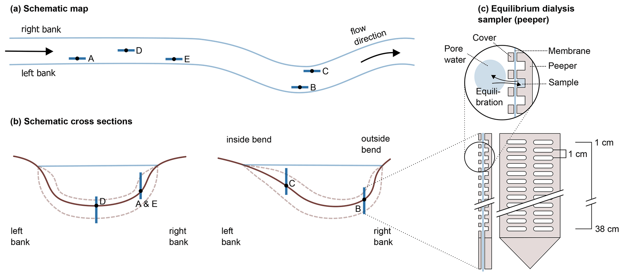
Figure 1 Schematic representation of the five sampling sites along the river (a) and across the riverbed (b). In panel (c), the sampler is schematically drawn, modified after Teasdale et al. (1995) (top: detail, bottom left: side view, bottom right: front view; for clarity, only 12 of the 38 chambers are illustrated).

2.2 Pore-water sampling with a sediment peeper

High-resolution geochemical depth profiles were obtained at each sampling site with an in situ equilibrium dialysis sampler (peeper) as described by Hesslein (1976) (see Fig. 1c). The body of the peeper was equipped with two rows of 38 chambers with a spatial depth resolution of 1 cm. All chambers were filled with deionized water, covered with a semi-permeable polysulfone membrane with a pore diameter of 0.2 µm (Pall Corporation, Dreieich, Germany), and fixed with a Plexiglas cover and plastic screws. At each sampling site, the peeper was pushed manually into the stream bed until most chambers were buried in the sediment and only the uppermost chambers had contact with river water. To minimize flow disturbance, peepers were oriented longitudinally to the flow direction as indicated in Fig. 1a.

An equilibrium between the water in the chambers and the surrounding pore water was obtained by diffusion of dissolved molecules through the membrane during a time period of at least 3 weeks. This exceeds the recommended equilibration time of a minimum of 2 weeks (Teasdale et al., 1995). The extended equilibration time was chosen to allow for recovery of natural geochemical gradients after the disruption caused by placing the peeper. Pore-water samples represent an average of pore-water concentrations during the sampling period, and diurnal or other short-term temporal fluctuations during this time cannot be detected.

For sampling, the peeper was removed from the sediment and cleaned with deionized water. The first column of chambers was used for oxygen measurements and withdrawal of samples for determination of ion concentrations, and the second column was used for CH₄ concentration measurements and analyses of stable carbon isotopes of CH₄. A Clark-type microsensor (Unisense A/S, Aarhus, Denmark) was pierced through the membrane for immediate measurements of dissolved O₂ in the field. The O₂ measurements were conducted on site within 10 min after removal of the peeper from the sediments to avoid contamination with atmospheric O₂. Liquid samples were then drawn from the same chambers with 5 mL syringes.

The 10 mL glass vials for CH₄ concentration measurements and stable carbon isotope analysis (δ¹³C–CH₄) were prepared in the laboratory with 20 µL 10 M NaOH, sealed with rubber butyl stoppers and flushed for at least 2 min with synthetic air (O₂, N₂) to remove background atmospheric CH₄. Immediately before sample injection, a small needle was pushed through the stoppers to allow pressure exchange. Subsequently, with a syringe and needle samples were injected slowly along the side of the vial to avoid degassing. Both needles were removed directly after sample injection. To avoid CH₄ losses to the atmosphere through the membrane, sampling was conducted quickly within 15 min after removal from the sediment. Nevertheless, small amounts of CH₄ could diffuse out through the membrane or escape during sample injection, and thus, measured CH₄ concentrations might be slightly underestimated. Samples for ion concentrations were collected in 1.5 mL glass vials and prepared with 10 µL 0.5 M NaOH for anion analysis (Cl⁻, NO${}_{\mathrm{3}}^{-}$, NO${}_{\mathrm{2}}^{-}$, SO${}_{\mathrm{4}}^{\mathrm{2}-}$) or 10 µL 1 M HNO₃ for cation analysis (NH${}_{\mathrm{4}}^{+}$). All samples were withdrawn within 45 min after removal of the peeper. The samples were transported to the laboratory in a cooler and stored refrigerated prior to analysis.

2.3 Chemical and isotopic analyses

2.3.1 Anion and cation measurements

Anion and cation concentrations were determined using ion chromatography, specifically a system of two Dionex ICS-1100 systems (Thermo Fisher Scientific, Dreieich, Germany) equipped with Dionex IonPac™ AS9-HC and CS12A columns for anion and cation separation, respectively. Measurements were performed in triplicates and evaluated on the basis of seven concentration standards (Merck KGaA, Darmstadt, Germany). Concentrations are given as mean values of the triplicates. Analytical uncertainty was <10 %, and detection limits were 0.020 mmol L⁻¹ for Cl⁻, 0.012 mmol L⁻¹ for NO${}_{\mathrm{3}}^{-}$, 0.007 mmol L⁻¹ for NO${}_{\mathrm{2}}^{-}$, 0.008 mmol L⁻¹ for SO${}_{\mathrm{4}}^{\mathrm{2}-}$ and 0.005 mmol L⁻¹ for NH${}_{\mathrm{4}}^{+}$.

2.3.2 CH₄ concentrations and δ¹³C measurements of CH₄

Methods for CH₄ sampling and concentration measurements are further developments of standards introduced by the EPA (2001). Sample vials were equilibrated in a water bath at 30 ^∘C for at least 2 h before measurements of headspace CH₄ concentrations with a TRACE 1300 gas chromatograph (GC) (Thermo Fisher Scientific, Dreieich, Germany). The GC was equipped with a TG-5MS column and flame ionization detector (FID) and calibrated with three standards (Rießner-Gase GmbH, Lichtenfels, Germany). Triplicate measurements were performed through manual injection of 250 µL headspace gas. Total CH₄ concentrations in the water and gas phase of the sample vials were calculated with Henry's law according to the equilibrium headspace method first described by Kampbell and Vandegrift (1998).

The same sample vials were used for measuring ${}^{\mathrm{12}}\mathrm{C}{/}^{\mathrm{13}}\mathrm{C}$ ratios of CH₄ with cavity ring-down spectroscopy (CRDS), specifically the G2201-i gas analyzer with a Small Sample Introduction Module (SSIM) (Picarro Inc., Santa Clara, CA, USA) calibrated with two standards (Airgas, Plumsteadville, PA, USA). Reliable results could only be obtained for headspace CH₄ concentrations >30 ppm. This threshold concentration was found in previous experiments (Sect. S2). Due to the small available gas volume in the headspace of approximately 7 mL, dilution with synthetic air was necessary, and CH₄ concentrations in the analyzer decreased while repeating measurements. Values were only adopted when at least two of three measurements were above the threshold concentration. The standard δ notation is used for representing the results according to Eq. (1) relative to the VPDB (Vienna Pee Dee Belemnite) standard.

$$\begin{array}{}\text{(1)}& \mathit{\delta }\left[\mathrm{‰}\right]=\left({\displaystyle \frac{R_{\mathrm{Sample}}}{R_{\mathrm{Standard}}}}-\mathrm{1}\right)\times {\mathrm{10}}^{\mathrm{3}}\end{array}$$

2.4 Inverse modeling of concentration gradients

The one-dimensional numerical modeling software PROFILE, introduced by Berg et al. (1998), was used to support the interpretation of measured geochemical profiles. The software provides an objective procedure for finding the simplest production–consumption profile which accurately represents the measured concentration gradients. For this, concentration profiles are divided into different zones with constant production–consumption rates. Then, several best-fit results are produced by minimizing the sum of squared deviations (SSD), each representing a different number of these zones. Finally, best fits are compared using statistical F testing for finding the lowest number of zones which best describe the data.

The model assumes concentration gradients to represent a steady state (Berg et al., 1998), which neglects the fact that reaction rates in the HZ show temporal variability (Marzadri et al., 2012). However, the pore-water samples obtained with the sediment peeper represent a time-averaged state during the total sampling period of at least 3 weeks. The relative contribution of short-term fluctuations decreases with the length of the averaged time. Therefore, as a first approximation we assume that after 3 weeks this dynamic component is small particularly in the deeper HZ and can be neglected.

Boundary conditions (BCs) were set as follows: for O₂, NO${}_{\mathrm{3}}^{-}$ and SO${}_{\mathrm{4}}^{\mathrm{2}-}$ a fixed concentration was set at the top, and a zero-flux BC was set at the bottom of the profile; for CH₄ a fixed concentration and zero-flux BC were set at the top of the profile, similar to what was used by Norði and Thamdrup (2014). Positive production rates were only allowed for SO${}_{\mathrm{4}}^{\mathrm{2}-}$ and CH₄, while for O₂ and NO${}_{\mathrm{3}}^{-}$ only negative rates (consumption) were permitted. Bioturbation and irrigation were neglected. Molecular diffusion coefficients in water D⁰ (m² s⁻¹) were calculated based on Boudreau (1997) as a function of the average water temperature during the equilibration period. Sediment diffusion coefficients D_S were determined as a function of D⁰ based on an empirical relation (Iversen and Jørgensen, 1993). More details and calculated diffusion coefficients D⁰ and D_S are given in Sect. S3.

2.5 DNA extraction, qPCR and 16S rRNA gene sequencing

At location C, an additional sediment core was taken for depth-resolved microbiological analyses via DNA extraction, quantitative PCR and 16S rRNA gene sequencing. For this, a coring tube with an inner diameter of 42 cm was cut open lengthwise, cleaned with ethanol and distilled water, and closed again with tape. The core was taken by manually pushing the tube into the sediment right next to the peeper, pulling it out and transferring it to the laboratory. There, the tape was removed for opening the tube and allowing access to the sediment core. The sediment was split into 10 subsamples with a resolution of 2 cm in the upper 12 cm depth and 3 cm below. All samples were immediately frozen and stored at −22 ^∘C until further analysis.

For each sampled depth, we performed four biological replicates of DNA extraction. Total DNA was extracted from 0.5 g of sediment as previously described (Vuillemin et al., 2019). DNA templates were diluted to 1 : 100 in ultrapure PCR water (Roche, Germany) and used in qPCR amplifications with updated 16S rRNA gene primer pair 515F (5^′-GTG YCA GCM GCC GCG GTA A-3^′) and 806R (5^′-GGA CTA CNV GGG TWT CTA AT-3^′) to increase our coverage of archaea and marine clades and run as previously described (Pichler et al., 2018). All qPCR reactions were set up in 20 µL volumes with 4 µL of DNA template, 20 µL SsoAdvanced Universal SYBR Green Supermix (Bio-Rad, Feldkirchen, Germany), 4.8 µL nuclease-free H₂O (Roche, Germany), 0.4 µL primers (10 µM; biomers.net) and 0.4 µL MgCl₂ and carried out on a CFX Connect qPCR machine for gene quantification. For 16S rRNA genes, we ran 40 PCR cycles of two steps corresponding to denaturation at 95 ^∘C for 15 s, annealing and extension at 55 ^∘C for 30 s. All qPCR reactions were set up in 20 µL volumes with 4 µL of DNA template and performed as previously described (Coskun et al., 2019). Gel-purified amplicons of the 16S rRNA genes were quantified in triplicate using a Quant-iT dsDNA reagent (Life Technologies, Carlsbad, CA, USA) and used as a standard. An epMotion 5070 automated liquid handler (Eppendorf, Hamburg, Germany) was used to set up all qPCR reactions and to prepare the standard curve dilution series spanning from 10⁷ to 10¹ gene copies. Reaction efficiency values in all qPCR assays were between 90 % and 110 % with R² values >0.95 for the standards.

For 16S rRNA gene library preparation, qPCR runs were performed with barcoded primer pair 515F and 806R as described previously (Pichler et al., 2018). In brief, 16S rRNA gene amplicons were purified from 1.5 % agarose gels using the QIAquick Gel Extraction Kit (Qiagen, Hilden, Germany), quantified with the Qubit dsDNA HS Assay Kit (Thermo Fisher Scientific, Dreieich, Germany), normalized to 1 nM solutions and pooled. Library preparation was carried out according to the MiniSeq System Denature and Dilute Libraries Guide (Illumina, San Diego, CA, USA). Sequencing was performed on the Illumina MiniSeq platform at the GeoBio-Center^LMU. We used USEARCH version 10.0.240 for MiniSeq read trimming and assembly, OTU (operational taxonomic unit) picking and 97 % sequence identity clustering (Edgar, 2013), which, as we showed previously, captures an accurate diversity represented within mock communities sequenced on the same platform (Pichler et al., 2018). OTU representative sequences were identified by BLASTn (nucleotide–nucleotide basic local alignment search tool) searches against SILVA database version 132 (Quast et al., 2012). To identify contaminants, 16S rRNA genes from extraction blanks and dust samples from the lab were also sequenced in triplicate (Pichler et al., 2018). These 16S rRNA gene sequences were used to identify any contaminating bacteria (e.g., Acinetobacter, Bacillus, Staphylococcus) and selectively curate the OTU table.

3 Results and discussion

3.1 Concentration profiles show steep geochemical gradients and the formation of a complex redox zonation

The geochemical profiles obtained in the HZ of the river Moosach are shown in Fig. 2. The total depth of the profiles depended on how deep the peeper was pushed into the ground and varied between 27 and 38 cm. Above the sediment–water interface, in-stream concentrations were 270–300 µmol L⁻¹ for dissolved O₂, 280–380 µmol L⁻¹ for NO${}_{\mathrm{3}}^{-}$, 240–360 µmol L⁻¹ for SO${}_{\mathrm{4}}^{\mathrm{2}-}$ and 1270–1650 µmol L⁻¹ for Cl⁻. Surface water concentrations as measured on the day of sampling are displayed as vertical beams above the sediment–water interface in Fig. 2.

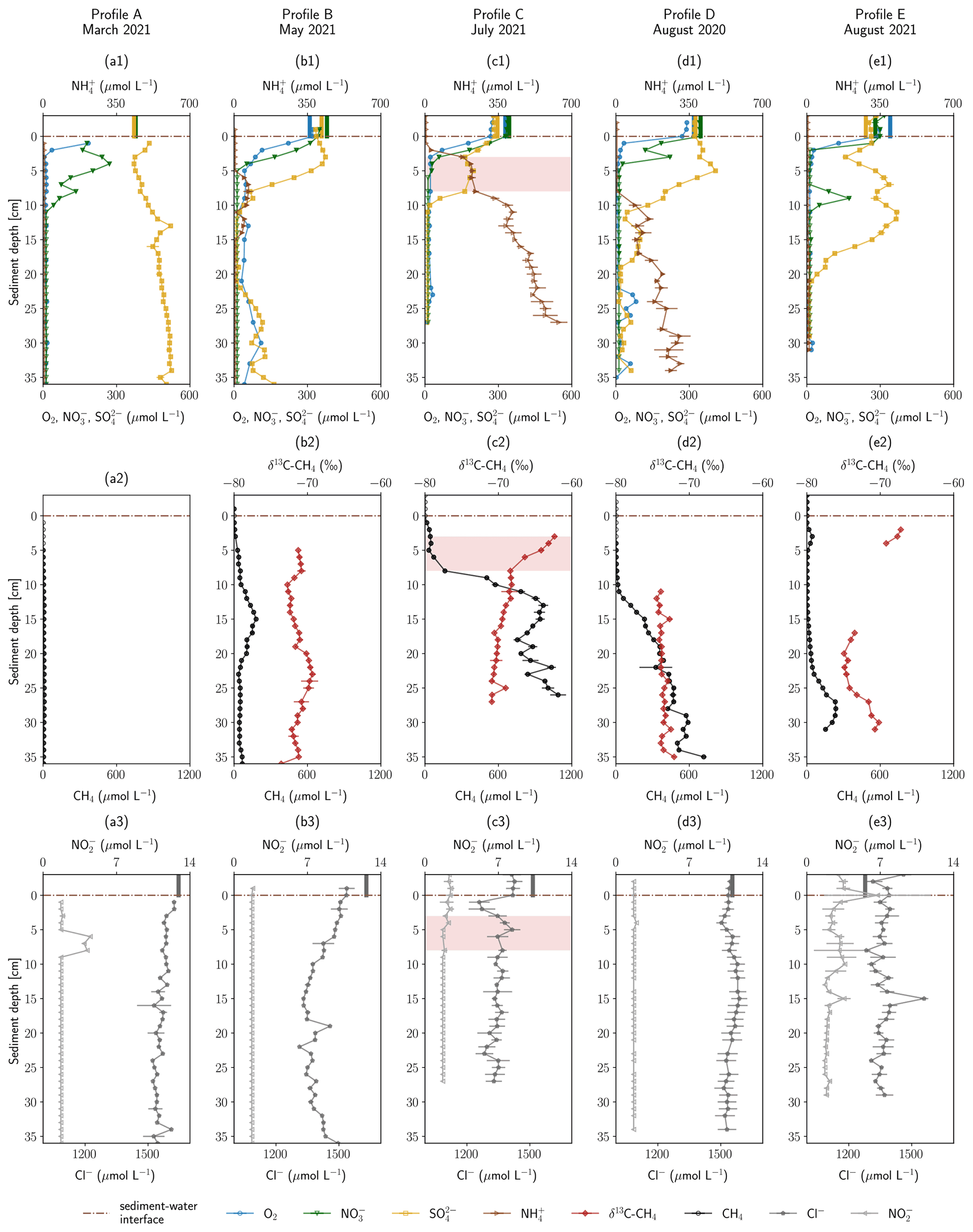
Figure 2 Depth-resolved profiles of hyporheic pore-water geochemistry at five sampling sites. Panels (a1) to (e1) show O₂, NO${}_{\mathrm{3}}^{-}$, NH${}_{\mathrm{4}}^{+}$ and SO${}_{\mathrm{4}}^{\mathrm{2}-}$ concentrations. Panels (a2) to (e2) show CH₄ concentrations and δ¹³C–CH₄ values. Panels (a3) to (e3) show NO${}_{\mathrm{2}}^{-}$ and Cl⁻ concentrations. Empty markers indicate values outside the range of used standards. Error bars show standard deviations of independent measurements (n=3). Vertical lines above the sediment–water interface are concentrations measured in the surface water at the sampling date. Red background color highlights an enrichment in δ¹³C–CH₄. Profiles are ordered by season.

Land use in the catchment is predominantly agriculture, and leaching of fertilizers presumably adds NO${}_{\mathrm{3}}^{-}$ to river and groundwater, but values stayed clearly below the threshold of the EU Nitrates Directive of 50 mg L⁻¹ (806 µmol L⁻¹). SO${}_{\mathrm{4}}^{\mathrm{2}-}$ concentrations in the surface water were strikingly high for a freshwater river, especially in spring. Groundwater in the quaternary aquifer, the groundwater body hydraulically connected to the river, showed SO${}_{\mathrm{4}}^{\mathrm{2}-}$ concentrations between 448 and 573 µmol L⁻¹ during 2007–2020 as measured in an observation well approximately 1.6 km southwest of the sampling sites (Bavarian State Office of the Environment, 2022). Peat can contain substantial amounts of carbon-bonded sulfur and pyritic sulfides (Spratt et al., 1987; Casagrande et al., 1977), and SO${}_{\mathrm{4}}^{\mathrm{2}-}$ can be released due to pyrite and organic matter oxidation (Vermaat et al., 2016), likely so in the drained moor areas in the foothills of the Munich gravel plain that the river Moosach crosses. In an agricultural watershed sulfur fertilizers can also be a source of elevated SO${}_{\mathrm{4}}^{\mathrm{2}-}$ concentrations in shallow aquifers (Spoelstra et al., 2021).

Below the sediment–water interface dissolved O₂ concentrations decreased within a few centimeters in all sampled profiles and remained at <10 µmol L⁻¹ deeper down with only a few exceptions. Steep O₂ gradients and anoxic conditions just below this narrow aerobic zone were to be expected because the river Moosach is strongly altered by human engineering including controlled discharge conditions; a very low gradient; slow flow velocities; and deposits of fine, organic-rich materials. In profile B, O₂ concentrations were higher compared to all other sites (20–80 µmol L⁻¹ below 3 cm depth). This may be due to higher surface water influxes in the coarser gravelly sediment as opposed to the fine deposits found at the other sites. However, even at 10–20 cm depth, where CH₄ concentrations peaked in a sedimentary layer dominated by silt, O₂ was present at concentrations between 20 and 60 µmol L⁻¹. These high O₂ concentrations appear to be rather implausible in this zone where CH₄ is produced through methanogenesis, a strictly anaerobic process. An explanation could, however, be a contamination with atmospheric O₂ during field measurements. Similarly, profile D shows anomalies in the O₂ data with concentration peaks at 23–26, 30 and 33 cm depth. These may also be attributed to measurement artifacts, since they are located deep in the methanogenic zone where strictly anoxic conditions generally prevail.

Similar to dissolved O₂, NO${}_{\mathrm{3}}^{-}$ concentrations decreased from 280–380 µmol L⁻¹ in river water to concentrations of <12 µmol L⁻¹ (detection limit) within a few centimeters. In contrast, the conservative tracer Cl⁻ did not disappear in a comparable manner, which may demonstrate that microbial consumption and not dilution or mixing was responsible for the development of these steep chemical gradients. A peak of NO${}_{\mathrm{2}}^{-}$ in profile A exactly where the NO${}_{\mathrm{3}}^{-}$ gradient is located (6–8 cm) indicates bacterial NO${}_{\mathrm{3}}^{-}$ reduction to NO${}_{\mathrm{2}}^{-}$, possibly as an intermediate in denitrification (Fig. 2a3). In profiles B–E O₂ reduction and denitrification zones were very close, and both gradients overlapped. Oxygen reduction and denitrification zones seem to be only millimeters wide, similar to what was described for other freshwater sediments in the literature (Raghoebarsing et al., 2006). In profile D a peak between 8–10 cm depth with a maximum of 173 µmol L⁻¹ stands out that coincides with a reduction in SO${}_{\mathrm{4}}^{\mathrm{2}-}$ concentrations.

SO${}_{\mathrm{4}}^{\mathrm{2}-}$ concentration profiles showed some distinctive features. In profiles A and B, concentrations slightly increased towards the bottom of the profile. This could be connected to the intrusion of upwelling, reduced groundwater with a higher SO${}_{\mathrm{4}}^{\mathrm{2}-}$ concentration compared to surface water. Rising Cl⁻ concentrations in the lower third of profile B support this interpretation, since they reach 1491 µmol L⁻¹, a value very similar to groundwater Cl⁻ concentrations of 1440–1495 µmol L⁻¹ in recent years (2016–2020) (Bavarian State Office of the Environment, 2022). Further, in profiles B and D, SO${}_{\mathrm{4}}^{\mathrm{2}-}$ concentrations increased in the upper parts of the profiles in 0–3 and 0–5 cm depth, respectively, and also in profile E between 3–7 and 9–11 cm depth. Here, a biogeochemical source, for example re-oxidation of H₂S traveling upwards from more reduced zones, could explain the observed trends. Below, in 3–11 cm (profile B), 5–11 cm (profile C) and 12–22 cm depth (profile E), concentrations declined, potentially through bacterial SO${}_{\mathrm{4}}^{\mathrm{2}-}$ reduction. This interpretation is supported by a sulfidic smell during sampling. Interestingly, in profile C SO${}_{\mathrm{4}}^{\mathrm{2}-}$ concentrations decreased significantly not only between 8–11 cm but also between 0–3 cm depth, concurrently with decreases in O₂ and NO${}_{\mathrm{3}}^{-}$ concentrations. One possible interpretation is a dilution effect at the clogged sediment surface, as also suggested by simultaneous decreases in Cl⁻ (Fig. 2c3) and Ca²⁺ (data not shown) concentrations. But the data could also show the co-occurrence of oxic and anoxic micro-niches in close proximity, a situation that has also been described previously (Storey et al., 1999; Triska et al., 1993).

NH${}_{\mathrm{4}}^{+}$ concentrations in most profiles (C–E) consistently increased with sediment depth. While maximal concentrations in profiles C and D were 116 and 308 µmol L⁻¹, respectively, in profile C values reached a level of > 1000 µmol L⁻¹. During biodegradation of organic matter, NH${}_{\mathrm{4}}^{+}$ is released when nitrogenous compounds are transformed through ammonification (Ladd and Jackson, 1982). Increases with depth show progressive decomposition, and high NH${}_{\mathrm{4}}^{+}$ concentrations can be seen as a proxy for a high content of microbially degraded organic matter in the sediment. Thus, organic carbon content seems to be significantly lower in location E compared to C and D. In location A, NH${}_{\mathrm{4}}^{+}$ concentrations even stayed below the detection limit (<5 µmol L⁻¹). Profile B has elevated NH${}_{\mathrm{4}}^{+}$ concentrations in 6–14 cm depth and values below the detection limit elsewhere.

Similar to NH${}_{\mathrm{4}}^{+}$ concentrations, CH₄ concentrations generally increased with depth and were highest in profile C, followed by profile D. In profile A, where NH${}_{\mathrm{4}}^{+}$ concentrations were lowest compared to all other profiles, CH₄ concentrations stayed below 10 µmol L⁻¹. More complex were the observed CH₄ gradients in profiles B and D. In profile B, CH₄ peaked at a concentration of 180 µmol L⁻¹ in a sediment depth of 15 cm. Below, from 23 cm onwards, concentrations decreased and stayed around 50 µmol L⁻¹. CH₄ concentrations of profile E revealed a small peak (44 µmol L⁻¹) at 3 cm depth, showed very low concentrations of <10 µmol L⁻¹ between 5–15 cm and rose again up to 237 µmol L⁻¹ at a depth of 28 cm.

Generally, a tendency of increasing CH₄ concentrations with higher surface water temperatures can be observed. Profiles A and B, measured in spring, showed significantly lower CH₄ concentrations than those sampled in summer. However, comparing profiles C, D and E, all measured in summer, substantial differences in total CH₄ concentrations are eye-catching. By far the highest CH₄ concentrations were measured in July 2021 (T_M=16.6 ^∘C for profile C, Table S1 in the Supplement), although surface water temperatures were slightly lower than in August 2020 (T_M=17.1 ^∘C for profile D). Pore-water CH₄ concentrations did not exceed CH₄ saturation concentrations of at least 2.1 mmol L⁻¹ (calculated using PHREEQC, Parkhurst and Appelo, 2013, for the mean surface water temperature during the sampling periods and respective water depths at each site) with only one exception. In profile C, a CH₄ concentration of 19.8 mmol L⁻¹ was measured in 27 cm depth (not displayed in Fig. 2, since it is far out of the axes' range), which exceeds the saturation concentration by far and implies direct contact with a gas bubble. In addition, it must be mentioned that bubble formation is also possible at lower CH₄ partial pressures if microstructures are present or if CH₄ production occurs in small-scale local hotspots. In comparison, profile E, measured in August 2021, exhibits low concentrations despite the summer temperatures (T_M=15.8 ^∘C). Varying organic matter contents at the three sites might explain these differences and seems to be a determining parameter for total CH₄ production, as inferred from differences in NH${}_{\mathrm{4}}^{+}$ concentrations. When complex organic molecules are degraded by microbes, NH${}_{\mathrm{4}}^{+}$ is not only released but also educts for methanogenesis like H₂, CO₂, acetate and methylated compounds like methanol (Capone and Kiene, 1988). The degradation of organic carbon is therefore a driver of methanogenesis, and we see a correlation between CH₄ and NH${}_{\mathrm{4}}^{+}$ concentrations (see Fig. S4). This finding is also consistent with previous reports from stream sediment incubations (Bodmer et al., 2020; Romeijn et al., 2019; Bednařík et al., 2019).

Cl⁻ can be viewed as a conservative tracer. As mentioned above, one irregularity is a sudden concentration decrease in the first centimeters of profile C. This could show the effect of clogging because fine deposits fill the pore space and reduce hyporheic exchange. Interesting is also that Cl⁻ concentrations decrease in the middle section of profile B. Cl⁻ concentrations in profiles A, D and E do not exhibit any trends; fluctuations are highest in profile E.

3.2 Explaining redox zones with sediment heterogeneities and hyporheic exchange fluxes

Observed concentration profiles at the different stream sites showed distinct characteristics and were very heterogeneous. The divergence of the profiles becomes particularly clear when comparing profiles A and E that show hardly any similarities although they were sampled at two very similar sites. In March, where river water is well oxygenated with average surface water temperatures of 7.5 ^∘C (profile A), SO${}_{\mathrm{4}}^{\mathrm{2}-}$ concentrations were high (>300 µmol L⁻¹) throughout the profile, and almost no CH₄ was produced. In August (profile E), clear gradients in SO${}_{\mathrm{4}}^{\mathrm{2}-}$ and CH₄ concentrations together with nearly constant Cl⁻ concentrations point towards a high activity of SRB (sulfate-reducing bacteria) and methanogens. As mentioned earlier, higher stream water temperatures in summer (profile E) could be the reason for higher microbial activity compared to early spring (profile A). However, the influence of temperature on GHG emissions from rivers has been discussed controversially. Increasing GHG production with rising temperatures was observed in laboratory incubations of river sediments (Comer-Warner et al., 2018; Shelley et al., 2015), while Silvennoinen et al. (2008) found that 55 % of all CH₄ emissions from the Temmesjoki River were released during winter time.

In our data, temperature alone may not explain the differences between the two profiles A and E. Concentration gradients in profile E do not follow the generally known redox zonation (Canfield and Thamdrup, 2009). The assumption that stream water enters the HZ at the sediment–water interface and that electron acceptors are consumed successively can explain neither the complex SO${}_{\mathrm{4}}^{\mathrm{2}-}$ dynamics nor the deep NO${}_{\mathrm{3}}^{-}$ peak. A possible reason could be surface water entering the sediment bank from the side, maybe in a sandier layer, such that sample depths represent different and varying flow path lengths of hyporheic fluxes. This is further illustrated in Fig. 3e. Stream water entering the bank from the side could be an additional reason (besides cold temperatures and potentially low organic matter degradation) for low CH₄ levels in profile A (Fig. 3a). Figure 3 schematically shows the hypothesized sedimentary characteristics and potential hyporheic fluxes at all five sampling sites.

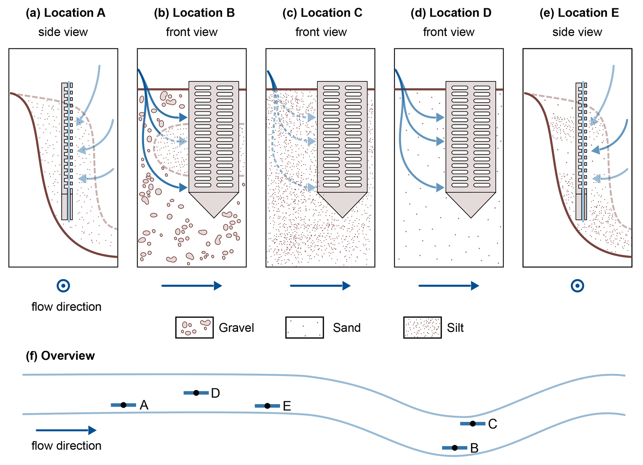
Figure 3 Schematic representation of potential hyporheic flow paths (blue arrows) at the five sampling sites. For locations A and E, a side view was chosen, and for locations B, C and D a front view was used. Where the front view is shown, flow direction in the river is from left to right, and where the side view is shown, flow direction is out of the drawing plane. The color strength of the arrows corresponds to the expected magnitude of hyporheic fluxes. The sediment composition is schematically indicated. Quantitative data on the sediment composition at the five locations can be found in Sect. S1.

Sediment stratification and resulting hyporheic fluxes can also help in understanding profile B. In the top section, as would be expected, O₂, NO${}_{\mathrm{3}}^{-}$ and SO${}_{\mathrm{4}}^{\mathrm{2}-}$ are consumed consecutively, and CH₄ concentrations rise, but below 15 cm depth, we see the reverse trends. A lens of fine material in an otherwise gravelly sediment would be a plausible explanation for this observation (Fig. 3b). In fact, very fine sediment was found below 11 cm depth, with gravel above, but the sediment core did not cover the lowest part of the profile (Sect. S1). Hyporheic flow velocities outside the fine lens would be faster than inside, and thus, although path lengths at the bottom are longer, contact times have been shorter than in the central part of the profile. This would mean that we see the methanogenic zone in the central part and the sulfate reduction zone at the bottom of profile B, depending on the available time for reactions along the flow path.

Also profile C deviated from the commonly assumed redox zonation. Bacterial SO${}_{\mathrm{4}}^{\mathrm{2}-}$ reduction appeared to occur concurrently with O₂ reduction and denitrification, possibly in co-occurring oxic and anoxic zones (Storey et al., 1999). Alternatively, this may be caused by dilution effects in the upper centimeters of the profile. Also unexpected were stagnating SO${}_{\mathrm{4}}^{\mathrm{2}-}$ concentrations with a slightly convex concentration gradient between 3–8 cm depth. There might be an additional SO${}_{\mathrm{4}}^{\mathrm{2}-}$ source, maybe recycling of reduced sulfur species from deeper zones or some cryptic sulfur cycling as has been suggested in the context of S-DAMO in freshwater environments (Ng et al., 2020; Norði et al., 2013). But also here, heterogeneous flow paths, for example due to wood and plant parts, could affect measured profiles such that water travel times do not linearly increase with depth.

The profile most clearly following the thermodynamic sequence was profile D. Here, O₂ was consumed first, followed by NO${}_{\mathrm{3}}^{-}$ and SO${}_{\mathrm{4}}^{\mathrm{2}-}$. Only after all other electron acceptors were consumed, CH₄ concentrations began to rise with depth.

When discussing the influence of hyporheic fluxes on redox zonation, it needs to be noted that not only spatial heterogeneities but also temporal dynamics may play a key role. For example, extreme events can alter the chemistry of infiltrating surface water, as well as hyporheic flow path lengths and residence times, thus impacting hyporheic geochemistry in multiple ways (Zimmer and Lautz, 2014). In this study in particular, location C might have been impacted by two high-flow events during the sampling period. Further, seasonal changes in river–groundwater mixing can potentially impact redox conditions and microbial populations (Danczak et al., 2016). However, fine sediments have been shown to reduce hyporheic exchange (Sunjidmaa et al., 2022). The combination of very fine deposits and stable, controlled hydrologic conditions is expected to limit hyporheic exchange and may also temper temporal dynamics in the HZ of the river Moosach.

3.3 Stable carbon isotopes of CH₄ reveal the importance of hydrogenotrophic methanogenesis and the roles of diffusive versus biotic processes in reducing CH₄ concentrations beneath the sediment surface

Figure 2 also shows δ¹³C–CH₄ values for profiles B–E in panels a2 to e2. CH₄ concentrations at location A were too low for isotopic analyses. In profile B, δ¹³C–CH₄ values were on average −74 ‰. δ¹³C–CH₄ values were very similar but slightly shifted in a range of <3 ‰ with an increasing trend (top to bottom) between 5–8 and 10–23 cm depth and a decreasing trend between 8–12 and 23–31 cm depth. These variations were too small to be taken as an indication for any microbially mediated processes and could be explained by diffusion controlled isotope fractionation.

In profile C on the other hand, two sections are clearly evident (see Fig. 2c2). From bottom to top, between 27 and 8 cm depth, δ¹³C–CH₄ values increased almost linearly from −71 ‰ to −69 ‰; then the slope changed abruptly, and an isotopic enrichment from −69 ‰ to −62 ‰ can be seen between a sediment depth of 8 and 3 cm. Isotopically lighter ¹²CH₄ is transported and consumed faster than heavier ¹³CH₄, which leads to an isotopic enrichment of the remaining CH₄ pool in the heavier ¹³CH₄ (Whiticar et al., 1986). This isotopic shift towards heavier isotopes from 8 to 3 cm combined with decreasing CH₄ concentrations, therefore, clearly indicates microbial CH₄ consumption. Interestingly, the measured O₂ gradient lied above this zone (0–3 cm depth), while denitrification potentially occurred in exactly this depth (0–5 cm), and SO${}_{\mathrm{4}}^{\mathrm{2}-}$ concentrations stagnated around 176 µmol L⁻¹ in 3–8 cm depth. Inverse modeling and the microbial community distribution at location C may help in interpreting the details of CH₄ oxidation as outlined in detail below (Sect. 3.4 and 3.5). The zone of ¹³CH₄ enrichment in profile C, where CH₄ oxidation is inferred, is highlighted by a red background color in Figs. 2 and 4 to visually help in differentiating this zone from the rest of the profile. The slight isotopic enrichment of δ¹³C–CH₄ of a few per mil below, between 27 and 8 cm depth, is likely affected by diffusion-controlled stable isotope fractionation. It is striking that CH₄ concentrations steeply decrease already between 12 and 8 cm depth, beneath the zone of strong ¹³CH₄ enrichment. Apparently, microbial consumption only impacts the upper part of the gradient, while diffusive transport shapes the lower part of the gradient.

In profile D, δ¹³C–CH₄ values were on average −71 ‰, and the isotopic composition stayed nearly constant. At least above 10 cm depth, where CH₄ concentrations were high enough for repeated isotope measurements, results suggest that microbial CH₄ oxidation did not play a key role in removing CH₄ from the HZ at location D. In profile E, reliable δ¹³C–CH₄ values could only be obtained in 2–4 and 17–21 cm depth. In the upper zone, values lay between −67 ‰ and −69 ‰, and in the lower zone, they were between −71 ‰ and −75 ‰, with a tendency towards less negative values in the lowest part of the profile. Since differences between isotope values at the top and the bottom were within a few per mil and there is a large data gap between 5–16 cm, data interpretations are difficult. The slightly heavier carbon isotopes of CH₄ at the top of the profile may be an indication for aerobic or anaerobic oxidation, but there is no additional evidence for this interpretation.

A kinetic isotope effect also occurs during CH₄ production and is larger for hydrogenotrophic than for acetoclastic methanogenesis (Krzycki et al., 1987). Here, δ¹³C–CH₄ values in the methanogenic zone were consistently lower than −60 ‰, which is characteristic for hydrogenotrophic methanogenesis (Whiticar, 1999). This fits well to findings of Bednařík et al. (2019) and Mach et al. (2015), who found that hydrogenotrophic methanogenesis was the dominant CH₄ production pathway in the HZ of the Elbe and Sitka rivers.

At all sampling sites CH₄ concentrations decreased towards the sediment surface, but in most of the profiles, where δ¹³C–CH₄ data were available, this was not accompanied by a significant enrichment in the heavier ¹³CH₄. Diffusive processes in these cases appear to be responsible for reducing CH₄ concentrations between the methanogenic zone and the upper part of the riverbed. At the sediment–water interface only very low CH₄ concentrations were found in all profiles (A–E), pointing towards small diffusive fluxes across the sediment–water interface. This finding is surprising because we expected high CH₄ concentrations and large fluxes to the water column and towards the atmosphere. However, it must be noted that we looked at diffusive CH₄ fluxes within the HZ and did not cover the possible generation and transport of gas bubbles. The contribution of these bubbles to total CH₄ fluxes across the sediment–water interface at the river Moosach remains unknown, but ebullition might be a significant contributor to CH₄ effluxes as suggested in the literature (DelSontro et al., 2010; McGinnis et al., 2016).

As explained above, isotopic evidence indicated a significant contribution of microbial CH₄ consumption to a reduction in diffusive CH₄ fluxes only in profile C. In all other profiles, it is possible either that CH₄ is oxidized at rates too low to alter its isotopic composition or that CH₄ oxidation takes place close to the sediment–water interface where CH₄ concentrations were too low for the isotope measurements. In both cases, this implies a limited relevance for the reduction in diffusive CH₄ fluxes. To gain further insights into aerobic and anaerobic CH₄ oxidation, the modeling software PROFILE was applied (Sect. 3.4). One reason for the observed methane oxidation processes in location C could be an increased supply of O₂ and NO${}_{\mathrm{3}}^{-}$ during the two high-flow events in the sampling period.

3.4 Inverse modeling of concentration gradients as a basis for discussing aerobic versus anaerobic oxidation of CH₄

Figure 4 shows the results of inverse concentration gradient modeling with the software tool PROFILE. Overall, the modeled and measured concentrations agreed well to each other, especially for CH₄ and SO${}_{\mathrm{4}}^{\mathrm{2}-}$. In the more complex CH₄ and SO${}_{\mathrm{4}}^{\mathrm{2}-}$ profiles, often several consumption zones were detected. Deviations of modeled from measured data were more pronounced for O₂ gradients in profiles B and D, as well as for the NO${}_{\mathrm{3}}^{-}$ gradient in profile E. Here, the model could not capture the data well, potentially because higher concentration values and outliers in deeper sediment depths might have biased the fit in the upper gradient, resulting in broader oxygen reduction and denitrification zones.

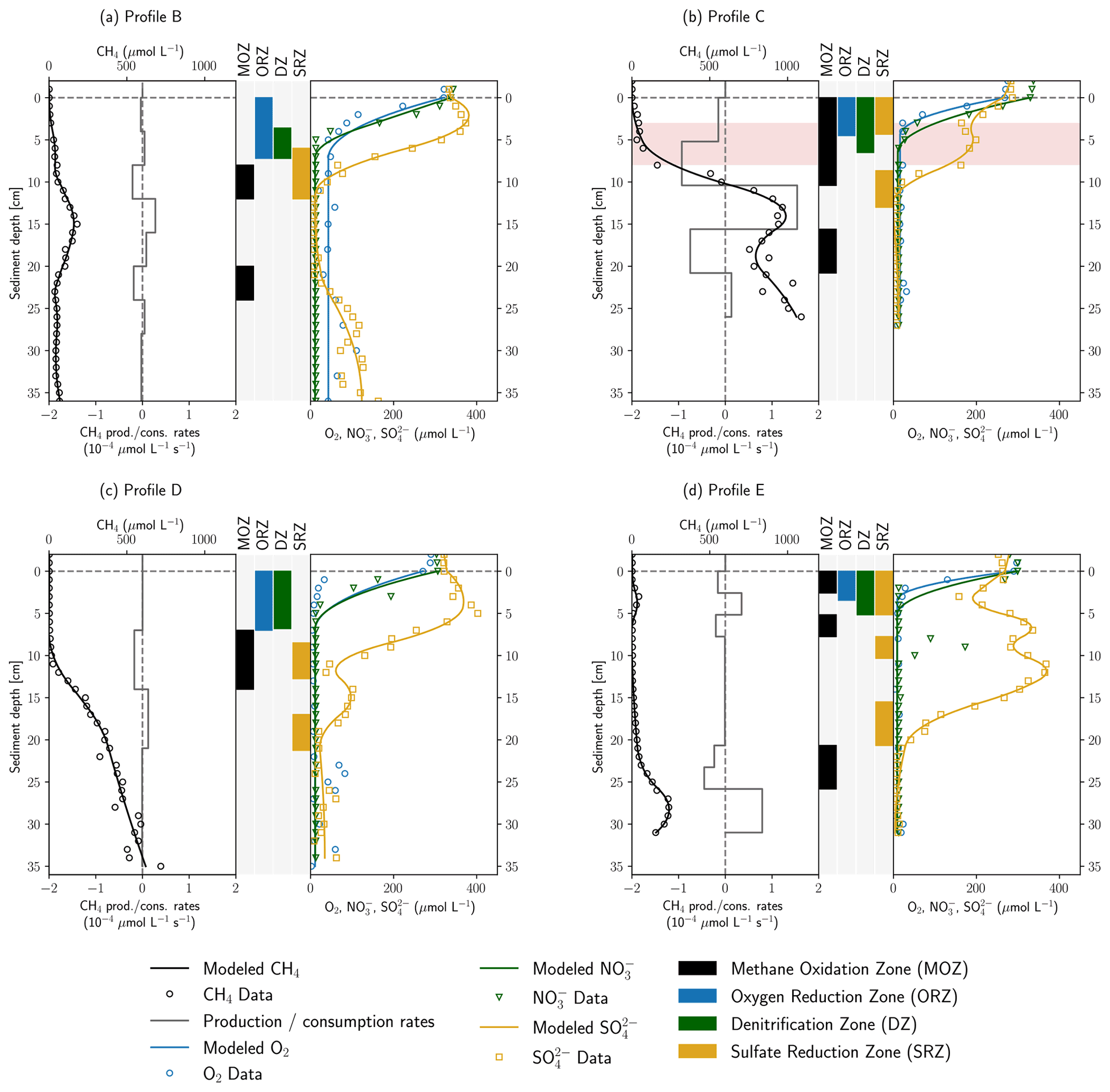
Figure 4 Results of concentration gradient modeling using the PROFILE software for profiles B–E. In panels (a)–(d), the left side shows modeled and measured CH₄ concentrations as well as modeled CH₄ production and consumption rates. In the center, the depth ranges of MOZ, ORZ, DZ and SRZ are highlighted. Zones with very low consumption rates ($<\mathrm{5}\times {\mathrm{10}}^{-\mathrm{6}}$ µmol L⁻¹ s⁻¹) were not identified. On the right, measured and modeled O₂, NO${}_{\mathrm{3}}^{-}$ and SO${}_{\mathrm{4}}^{\mathrm{2}-}$ concentrations are shown. Rates are not displayed for electron acceptors for reasons of clarity. Red background color in panel (b) highlights an enrichment in δ¹³C–CH₄.

In the PROFILE software, vertical transport can be attributed to diffusion, bioturbation and irrigation. However, exchange flows control riverbed biogeochemistry and solute transport in the HZ (Bardini et al., 2012, 2013). As a result, the disregard of advective solute transport with hyporheic exchange flows may lead to an underestimation of O₂, NO${}_{\mathrm{3}}^{-}$ and SO${}_{\mathrm{4}}^{\mathrm{2}-}$ reduction rates, since entering surface water increases the availability of educts for geochemical reactions. Where pore-water movement is slow, O₂ uptake is proportional to the rate of solute influx (Rutherford et al., 1993, 1995). On the other hand, CH₄-rich pore water is diluted with stream water, and modeled CH₄ oxidation rates may, therefore, rather be overestimated. Yet, hydraulic conductivities as calculated using the empirical formula of Beyer (1964) are relatively low ($<\mathrm{8}\times {\mathrm{10}}^{-\mathrm{5}}$ m s⁻¹) in the fine-grained deposits of the river Moosach (Table S4), which reduces the influence of the advective component in locations A, C and E. The model is applied to find the depths of reactive production and consumption zones. Calculated reaction rates are used to compare profiles, but due to the limitations described above, absolute values should not be overinterpreted.

Depth-integrated modeled O₂ consumption rates were in the range 0.10–0.41 mmol m⁻² d⁻¹. NO${}_{\mathrm{3}}^{-}$ reduction rates were found to be between 0.18 and 0.29 mmol m⁻² d⁻¹ in profiles C, D and E, while only 0.08 mmol m⁻² d⁻¹ of NO${}_{\mathrm{3}}^{-}$ was consumed in profile B in a much narrower DZ (denitrification zone). Using PROFILE for the interpretation of concentration gradients in a microcosm study, Norði and Thamdrup (2014) found rates of 11.4 mmol m² d⁻¹ for O₂ and 0.9 mmol m² d⁻¹ for NO${}_{\mathrm{3}}^{-}$ uptake, which is about 30–100 times higher for O₂ and 3–12 times higher for NO${}_{\mathrm{3}}^{-}$ than simulated here. In their work both O₂ and NO${}_{\mathrm{3}}^{-}$ were consumed completely within millimeters building much steeper gradients than observed in this study. Modeled ORZs (oxygen reduction zones) in profiles C and E were 4.5 and 3.5 cm wide; in profiles B and D they were even 7 cm, in the latter two cases partly due to poor fits. Additionally, as mentioned above, an underestimation of modeled O₂ and NO${}_{\mathrm{3}}^{-}$ uptake rates is likely, since the model does not include advective hyporheic exchange fluxes. In profile C, stream water can easily enter the sandy stream bed, and flow velocities are expected to be higher than close to the banks; O₂ uptake and denitrification are supposed to be much larger than suggested by the diffusive model.

In profile B a single SRZ (sulfate reduction zone) was found in 6–12 cm depth, whereas SO${}_{\mathrm{4}}^{\mathrm{2}-}$ reduction takes place in several depth ranges in profiles C–E. Total modeled SO${}_{\mathrm{4}}^{\mathrm{2}-}$ consumption ranged from 0.06 mmol m⁻² d⁻¹ (profile D) to 0.43 mmol m⁻² d⁻¹ (profile E). This is in line with modeling results of Norði et al. (2013), who found 0.2 mmol m⁻² d⁻¹ sulfate reduction in a freshwater lake sediment. Yet, directly measured rates were 10 times higher in their study, showing a discrepancy between modeled and measured values. Jørgensen et al. (2001) found SO${}_{\mathrm{4}}^{\mathrm{2}-}$ reduction rates of 0.65–1.43 mmol m⁻² d⁻¹ in the Black Sea using the same model. In profiles B and D SRZs were located beneath the ORZ and DZ, as would be expected, but in profiles C and E the uppermost SRZ overlapped with the ORZ and DZ. For profile C, the concurrent decrease in O₂, NO${}_{\mathrm{3}}^{-}$ and SO${}_{\mathrm{4}}^{\mathrm{2}-}$ has already been discussed in Sect. 3.1 (anaerobic micro-niches or dilution effects at a clogged sediment surface). For profile E, NO${}_{\mathrm{3}}^{-}$ is completely consumed between 1–2 cm depth in a very narrow DZ, and SO${}_{\mathrm{4}}^{\mathrm{2}-}$ concentrations start to decrease from 1 cm onwards, most likely right after NO${}_{\mathrm{3}}^{-}$ has been removed from the system. The model did not capture these very steep gradients precisely because data resolution was too coarse. Likewise, the sudden NO${}_{\mathrm{3}}^{-}$ peak in 9 cm depth in profile E was not recognized because too few data points in the peak were available.

MOZs (methane oxidation zones) were found in every profile even where δ¹³C–CH₄ values were stable, but rates were generally low ($<\mathrm{2}\times {\mathrm{10}}^{-\mathrm{4}}$ µmol L⁻¹ s⁻¹). For example, in profiles B and E, CH₄ was modeled to be consumed on both sides of the peaks in 3 and 15 cm depth, at rates of 0.06–0.07 mmol m⁻² d⁻¹ and 0.04–0.05 mmol m⁻² d⁻¹, respectively. It is not surprising that these small consumption rates did not change the isotopic composition of CH₄. A single MOZ was found in profile D in 7–14 cm depth with a depth-integrated rate of 0.11 mmol m⁻² d⁻¹. In profile C, 0.42 mmol CH₄ m⁻² d⁻¹ were simulated to be oxidized between 0–10.4 cm depth but with a 6 times higher rate below the ORZ (5.2–10.4 cm). This upper MOZ falls together with the observed enrichment in δ¹³CCH₄ between 3–8 cm depth.

The model was applied to help in identifying the electron acceptors responsible for CH₄ oxidation. This involves checking for overlaps between the MOZ and ORZ, DZ and SRZ. In profiles A and D, the MOZ only overlaps the SRZ combined with very low modeled oxidation rates. Profiles C and E show overlaps of all zones in the uppermost centimeters where δ¹³C–CH₄ measurements were not available due to low CH₄ concentrations. Here, aerobic methane oxidation could potentially take place.

In profile C, the modeled oxidation rate increased significantly below the ORZ and intersected with the DZ in the upper and the SRZ in the lowest part. This could point towards AOM coupled to denitrification or bacterial sulfate reduction in anoxic micro-niches, but since gradients were very steep and trace oxygen might also have been present, the delineation of the relevant electron acceptor is not possible. The higher CH₄ oxidation rate in the presence of NO${}_{\mathrm{3}}^{-}$ compared to O₂ in profile C, if valid, may show a situation in the HZ of the river Moosach similar to sediments of Lake Constance. Measurements of Deutzmann et al. (2014) showed that N-DAMO was the major CH₄ sink, although the community of aerobic methanotrophs would have been capable of oxidizing the entire methane flux. Limiting for aerobic oxidation was the available CH₄ after passing through the denitrification zone where most of it was already oxidized. Nonetheless, it is also possible that aerobic methane oxidation has a greater influence than suggested by the model. Either way, both aerobic and anaerobic CH₄ oxidation have the potential to reduce GHG emissions at location C.

Both profiles C and E have an additional MOZ deeper down where all electron acceptors were already consumed. In profile C it looks like the slope changes in the lower part of the profile are due to an overfitting of the model to fluctuating concentrations within the methanogenic zone. In profile D however, the deepest MOZ is located where CH₄ oxidation would be expected because of a clear slope change in the CH₄ concentration gradient. Potential electron acceptors could be SO${}_{\mathrm{4}}^{\mathrm{2}-}$, which is present only a few centimeters above; Fe or Mn oxides; or perhaps trace amounts of O₂.

3.5 Microbial communities at location C

The relative abundance of 16S rRNA gene sequences with similarity to known methanogenic microbial groups increased with sediment depth into the methane zone (Fig. 5a). In the shallower depths (0–4 cm) the methanogenic microbial community was dominated by the Methanomassiliicoccales and Methanofastidiosales, whereas at the bottom of the profile (16–21 cm) Candidatus “Methanomethyliales” and Methanomassiliicoccales dominated the methanogenic microbial community (Fig. 5b). The Methanomassiliicoccales and Candidatus “Methanomethyliales” both exhibit metabolic pathways in the genome indicative of H₂-dependent methylotrophic methanogenesis (Berghuis et al., 2019; Vanwonterghem et al., 2016). In saline or sulfate-rich environments, where methylated compounds like trimethyl amine or dimethyl sulfide are available as non-competitive substrates, this pathway can be of high importance (Conrad, 2020), but it is less considered in freshwater environments. However, Methanomassiliicoccales have been linked to CH₄ production from methanol in freshwater wetlands (Narrowe et al., 2019). Methanol can be derived from pectin, which is contained in terrestrial plants (Conrad, 2005), and thus, the combination of a high relative abundance of Methanomassiliicoccales combined with a high input of allochthonous plant material found in the sediment cores render this production pathway possible. The strong depletion in δ¹³C–CH₄ in the methanogenic zone supports the potential for CH₄ production from methanol. Carbon fractionation factors related to CH₄ production from methanol (ε_C = 68–77) are similar to those of hydrogenotrophic methanogenesis (ε_C = 55–58) and much higher than for acetoclastic methanogenesis (ε_C = 24–27) or CH₄ production from other methylated compounds (Whiticar, 1999). Candidatus “Methanomethyliales” is a newly discovered group of methanogenic archaea branching within Candidatus “Verstraetearchaeota” (Berghuis et al., 2019; Vanwonterghem et al., 2016). The increased relative abundance of Candidatus “Methanomethyliales” in our sediment core within the methane zone is the first clear piece of evidence that these novel methanogenic archaea could be important for CH₄ production in the HZ.

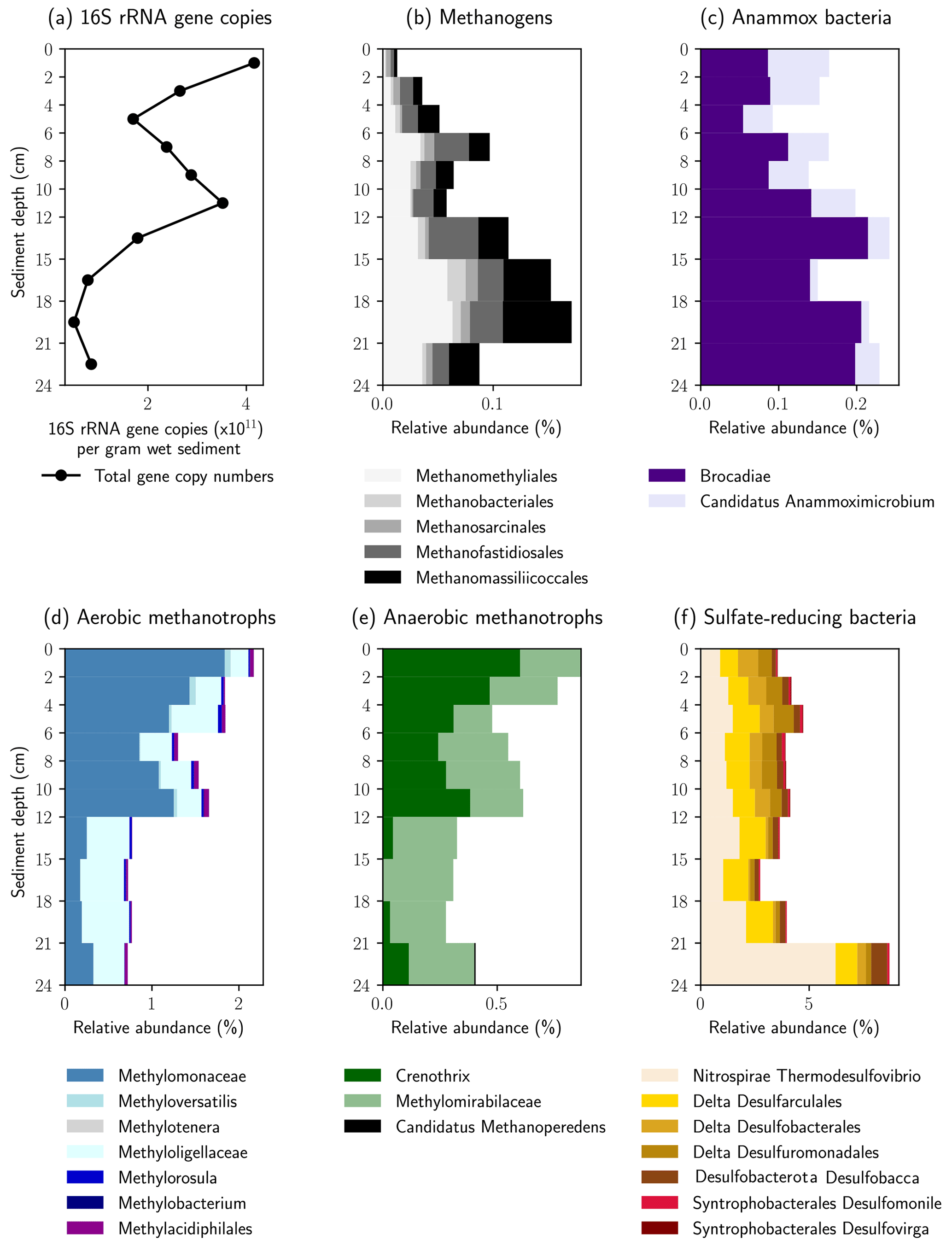
Figure 5 Relative abundance of key microbial groups detected in the 16S rRNA gene sequencing datasets. The histograms display the relative abundance (percentage of total reads) assigned to each group displayed. Note the increase in relative abundance of methanogenic groups below 12 cm, whereas the relative abundance of methane oxidizing groups increases above 12 cm.

Above the methane zone, there is an increased relative abundance of both aerobic and anaerobic CH₄ oxidizing microbial groups (Fig. 5d and e). The aerobic groups affiliated with Methylomonaceae (Gammaproteobacteria) and Methyloligellaceae (Alphaproteobacteria) dominated at depths above 12 cm (Fig. 5d) and are known to be involved in aerobic CH₄ oxidation (Takeuchi et al., 2019).

The anaerobic methanotrophs had the closest affiliation to Candidatus “Methylomirabilis” and Crenothrix. Both are involved in different steps of coupling CH₄ oxidation to the reduction of NO${}_{\mathrm{3}}^{-}$ and NO${}_{\mathrm{2}}^{-}$ (Oswald et al., 2017; Ettwig et al., 2010). The results indicate that anaerobic and aerobic CH₄ oxidizers can somehow inhabit the same sediment depths in the HZ, a finding that has been observed in paddy soil previously (Vaksmaa et al., 2017). Crenothrix is known to be a facultative anaerobe, which can explain its presence in oxic environments, but O₂ was shown to have a detrimental effect on members of Candidatus “Methylomirabilis” like Candidatus “Methylomirabilis oxyfera” (Luesken et al., 2012). Their high abundance in the uppermost centimeters of the sediment is, therefore, surprising. Yet, the close proximity and co-existence of aerobic and anaerobic CH₄ oxidizers fits well to the observed steep and partly overlapping gradients. The mixed distribution of strict anaerobes together with aerobes and facultative aerobes within the HZ could be due to mixing and turbidity at the stream bottom, which might resuspend and distribute sediments to different zones.

The presence of 16S rRNA gene sequences affiliated with the bacterial groups of Candidatus “Brocadia” and Candidatus “Anammoximicrobium”, which are known to perform anaerobic oxidation of ammonium (anammox) (Wu et al., 2020), may show that anammox via nitrite reduction was also ongoing. Because the anammox bacteria overlapped with anaerobic CH₄-oxidizing bacteria (Candidatus “Methylomirabilis” and Crenothrix) in the vertical profile, our results might show that, similar to anoxic lake bottom water (Einsiedl et al., 2020), a coupling of anammox with NO${}_{\mathrm{2}}^{-}$-dependent CH₄ oxidation (N-DAMO) is possible in the anoxic sediments of the HZ. This may represent a mechanism whereby N₂ is released and nitrogen is eliminated from the HZ. Based on the low abundance of ANME archaea we postulate that S-DAMO is unlikely to be a relevant process within the HZ of the river Moosach . This is also in line with earlier findings by Shen et al. (2019), who found that NO${}_{\mathrm{3}}^{-}$ and NO${}_{\mathrm{2}}^{-}$ could trigger AOM in all sandy river sediments in their study, while SO${}_{\mathrm{4}}^{\mathrm{2}-}$ and Fe were only effective in a few examples.

4 Conclusions

Measurements and interpretation of geochemical profiles and stable isotopes (δ¹³C–CH₄) at five different sampling sites in the river Moosach showed a predominant source of dissolved CH₄ and a potential for AOM. Based on our field study we confirm previous findings that large quantities of CH₄ are produced in river sediments, which can contribute to global warming. CH₄ was produced in all sampled locations, but CH₄ concentrations varied drastically between profiles. Much more CH₄ was produced in summer, especially in areas with fine, organic-rich sediments like inside bends of curved river sections. These findings suggest that the main influencing factors for CH₄ production in the HZ are temperature, organic carbon content and sediment composition. The uniqueness of the measured profiles underlines the high spatiotemporal variability in the hyporheic zone. Therefore, deriving general conclusions from point measurements is highly problematic, and the representativeness of the available data should be critically questioned in future research on CH₄ emissions from rivers.

Based on measured δ¹³C values and the microbial community found in location C, we consider hydrogenotrophic and H₂-dependent methylotrophic methanogenesis as relevant CH₄ production pathways. CH₄ concentrations at the sediment surface have been found to be low, and δ¹³C–CH₄ values were almost constant over the sampled sediment depth in most of the measured profiles, indicating a diffusion-limited transport of this GHG towards and across the sediment–water interface. However, in one of the profiles, an isotopic shift in δ¹³C–CH₄ to less negative values linked with decreasing CH₄ concentrations implied biological methane oxidation. Both microbiological and modeling methods showed the potential for anaerobic methane oxidation coupled with denitrification (N-DAMO). Yet, chemical gradients were very steep so that aerobic and anaerobic redox zones were in too close proximity to find a clear evidence for N-DAMO within the HZ of the river Moosach. Nevertheless, our results clearly show the removal of nitrogen and decreasing CH₄ concentrations towards the sediment–water interface. Both processes are crucial in improving the quality of river water and in reducing GHG emissions to the atmosphere.