the Creative Commons Attribution 4.0 License.
the Creative Commons Attribution 4.0 License.
 | 05 Oct 2022
Evaluation of soil carbon simulation in CMIP6 Earth system models
Sarah E. Chadburn
Eleanor J. Burke
Peter M. Cox
The response of soil carbon represents one of the key uncertainties in future climate change. The ability of Earth system models (ESMs) to simulate present-day soil carbon is therefore vital for reliably estimating global carbon budgets required for Paris Agreement targets. In this study CMIP6 ESMs are evaluated against empirical datasets to assess the ability of each model to simulate soil carbon and related controls: net primary productivity (NPP) and soil carbon turnover time (τs). Comparing CMIP6 with the previous generation of models (CMIP5), a lack of consistency in modelled soil carbon remains, particularly the underestimation of northern high-latitude soil carbon stocks. There is a robust improvement in the simulation of NPP in CMIP6 compared with CMIP5; however, an unrealistically high correlation with soil carbon stocks remains, suggesting the potential for an overestimation of the long-term terrestrial carbon sink. Additionally, the same improvements are not seen in the simulation of τs. These results suggest that much of the uncertainty associated with modelled soil carbon stocks can be attributed to the simulation of below-ground processes, and greater emphasis is required on improving the representation of below-ground soil processes in future developments of models. These improvements would help to reduce the uncertainty in projected carbon release from global soils under climate change and to increase confidence in the carbon budgets associated with different levels of global warming.
- Article
(18664 KB) - Full-text XML
- Companion paper 2
- Companion paper 3
-
Supplement
(694 KB) - BibTeX
- EndNote


Soil carbon is the Earth's largest terrestrial carbon store, with a magnitude of at least 3 times the amount of carbon contained within the atmosphere (Jackson et al., 2017). The response of soil carbon to CO2-induced global warming has the potential to provide a significant feedback to climate change, but this feedback is currently poorly known (Friedlingstein et al., 2006; Gregory et al., 2009; Arora et al., 2013; Friedlingstein et al., 2014; Arora et al., 2020; Song et al., 2021). Carbon stored within the atmosphere and global soils is exchanged via carbon fluxes as part of the global carbon cycle (Canadell et al., 2021). The Earth's terrestrial surface has acted as a carbon sink until now (Pan et al., 2011), but there is a possibility of a switch to a source during the 21st century, which would accelerate climate change (Cox et al., 2000; Crowther et al., 2016). Due to the significant quantities of carbon stored in soils globally, understanding and quantifying the potential release of carbon from soils is vital if the existing Paris Agreement targets are to be met (UNFCCC, 2015).
Earth system models (ESMs) are complex numerical models which simulate both climate and carbon cycle processes and are used to make projections of climate change. The latest generation of the Coupled Model Intercomparison Project (CMIP), CMIP6 (Eyring et al., 2016), includes an ensemble of ESMs, which are used in the most recent Intergovernmental Panel on Climate Change (IPCC) report (AR6) (IPCC, 2021). The relationships between carbon and environmental drivers used in models help to determine the response of the carbon cycle to climate change (Todd-Brown et al., 2013). Therefore, representing present-day carbon stores and spatial controls realistically within models is key for estimating carbon emission cuts required for Paris Agreement targets (Friedlingstein et al., 2022).
Present-day soil carbon can be approximately broken down into above-ground and below-ground controls, which influence the spatial distribution of soil carbon stocks (Koven et al., 2015). The above-ground control of soil carbon can be considered as the input flux of carbon into the soil from vegetation. Both the amount of carbon from plant and root litter (known as litterfall) and the fraction of this that is converted to longer-lived soil carbon pools will influence the storage of soil carbon. Net primary productivity (NPP) can be used as a proxy for the litterfall flux, where the fluxes are equal when vegetation is in a steady state. The below-ground control of soil carbon can be quantified simply in terms of the soil carbon turnover time (τs), which is defined as the time carbon resides in the soil (Koven et al., 2017; Carvalhais et al., 2014). τs can be considered as a proxy for below-ground controls on soil carbon storage (Koven et al., 2015).
In this study, the representation of late 20th century soil carbon stores and these related controls (NPP and τs) is evaluated in CMIP6 ESMs. Previously, similar studies have been conducted to evaluate soil carbon in the preceding generations of ESMs, for example, Anav et al. (2013) and Todd-Brown et al. (2013) for CMIP5. There are some existing CMIP6 soil-carbon-related studies; for example, Arora et al. (2020) evaluated carbon-concentration and carbon-climate feedbacks in 1 % CO2 yr−1 forcing simulations, Burke et al. (2020) evaluated the representation of permafrost in models, and Ito et al. (2020) investigated future soil carbon stocks under specific land use conditions. This study is the first to specifically focus on global and spatial soil carbon and related controls in CMIP6, with a thorough evaluation against empirical datasets and comparison against the preceding CMIP5 ensemble.
2.1 Earth system models
Soil carbon stores and related controls are examined in 11 CMIP6 ESMs (Eyring et al., 2016; Meehl et al., 2014), as listed in Table 1. Throughout the study, comparisons are made with 10 ESMs from the previous CMIP generation (CMIP5, Taylor et al., 2012), as listed in Table 2. The ESMs included in this study were chosen due to the availability of the required data in the online repository at the time of analysis (https://esgf-node.llnl.gov/search/cmip6/ (last access: 8 April 2022) https://esgf-node.llnl.gov/search/cmip5/, (last access: 12 April 2022)).
Ziehn et al. (2020)Haverd et al. (2018)Trudinger et al. (2016)Wu et al. (2019)Ji et al. (2008)Swart et al. (2019)Melton et al. (2020)Seiler et al. (2021)Danabasoglu et al. (2020)Lawrence et al. (2019)Séférian et al. (2019)Delire et al. (2020)Dunne et al. (2020)Zhao et al. (2018)Boucher et al. (2020)Cheruy et al. (2020)Guimberteau et al. (2018)Hajima et al. (2020)Ito and Oikawa (2002)Mauritsen et al. (2019)Goll et al. (2017)Goll et al. (2015)Seland et al. (2020)Lawrence et al. (2019)Sellar et al. (2020)Wiltshire et al. (2021)Table 1The 11 CMIP6 Earth system models included in this study and relevant features of their land carbon cycle components (Arora et al., 2020).

Table 2The 10 CMIP5 Earth system models included in this study and relevant features of their land carbon cycle components (Arora et al., 2013; Anav et al., 2013; Friedlingstein et al., 2014), including temperature and moisture functions presented in Todd-Brown et al. (2013).
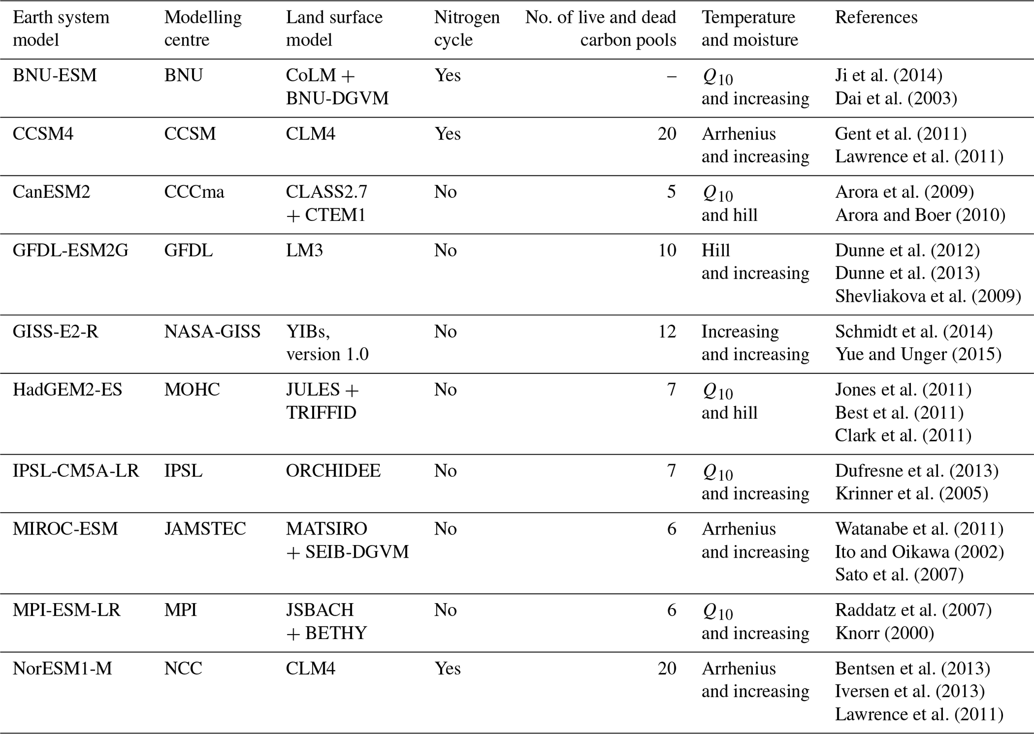
Tables 1 (CMIP6) and 2 (CMIP5) present information about the included ESMs, specifically more details about the associated land surface model (LSM). It should be noted that there are similarities between some of the LSMs – either advances from earlier models or even the same LSM within different ESMs. For example, CESM2 and NorESM2-LM both use the Community Land Model version 5 (CLM5) (Arora et al., 2020). For some modelling centres, both the CMIP5 and CMIP6 versions of the models are included, and in these cases direct comparisons can be made to determine changes from CMIP5 to CMIP6. These generationally related CMIP5 and CMIP6 models are CanESM2 and CanESM5, CCSM4 and CESM2, GFDL-ESM2G and GDFL-ESM4, IPSL-CM5A-LR and IPSL-CM6A-LR, MIROC-ESM and MIROC-ES2L, MPI-ESM-LR and MPI-ESM1.2-LR, NorESM1-M and NorESM2-LM, and HadGEM2-ES and UKESM1-0-LL, respectively. The models where only either the CMIP5 or CMIP6 version from the modelling centre was included are BNU-ESM and GISS-E2-R from CMIP5 and ACCESS-ESM1.5, BCC-CSM2-MR, and CNRM-ESM2-1 from CMIP6. A key general change to note is that CMIP6 has more models that include an interactive nitrogen cycle compared with CMIP5: ACCESS-ESM1.5, CESM2, MIROC-ES2L, MPI-ESM1.2-LR, NorESM2-LM, and UKESM1-0-LL in CMIP6 compared with CCSM4 and NorESM1-M in CMIP5 (the CMIP5 model BNU-ESM includes carbon–nitrogen interactions; however, this process was turned off in CMIP5 simulations; Ji et al., 2014). Additionally, an increased number of soil carbon pools is seen in some CMIP6 models (e.g. CLM5 has 29 carbon pools compared with 20 in CLM4). Arora et al. (2020) include a comprehensive overview of the updates seen in the individual CMIP6 models, which is presented in the “Model descriptions” section of the associated Appendix.
Todd-Brown et al. (2013) include a summary of the temperature and moisture dependencies of soil respiration/decomposition as assumed in the CMIP5 models (see Table 1 in Todd-Brown et al., 2013). The most common representation of the temperature sensitivity of decomposition is the Q10 equation, which is defined by , where T is temperature and T0 is a reference temperature. With the Q10 equation, decomposition increases exponentially with temperature (Davidson and Janssens, 2006). The majority of the other models used the Arrhenius equation to represent the temperature sensitivity, where the main difference from the Q10 representation is that decomposition levels off at higher temperature levels (Lloyd and Taylor, 1994). Of the remaining models, the GFDL model simulates an increased decomposition with temperature until some optimal temperature above which it decreases (Shevliakova et al., 2009) (which Todd-Brown et al., 2013, defined as a “hill” function) and the GISS model implements a linear increase in respiration to temperature up to a maximum value (Del Grosso et al., 2005). The representation of the decomposition sensitivity to soil moisture was found to be represented in two ways amongst the CMIP5 models, where decomposition was assumed either to increase monotonically with increasing soil moisture or less commonly to increase to some optimum moisture level and then decrease (again described as a “hill” function by Todd-Brown et al., 2013). In this study we note that the representation of temperature and moisture functions remains similar from CMIP5 to CMIP6. The Q10 equation remains the most common representation of soil temperature sensitivity in models, followed by the Arrhenius equation and then “hill” functions. Similarly, the most common representation of the sensitivity of soil to moisture in CMIP6 is a monotonically increasing function, followed by “hill” functions of various sorts.
2.2 Defining soil carbon variables
CMIP defines common output variables (Meehl et al., 2000), which allows for consistent comparison between the models and for cleaner evaluation of models against observational data. These common output variables also allow for consistent comparison between model generations, in this case between CMIP6 and CMIP5. This study focuses on evaluation of near-present-day soil carbon and related controls. Therefore the results presented in this study use the CMIP standard historical simulation (CMIP scenario historical) for both the CMIP6 and CMIP5 analyses. The historical simulation runs from 1850 to 2015 in CMIP6 and from 1850 to 2005 in CMIP5, where the selected dates for each variable (stated below) were chosen to allow for consistent comparison between CMIP5 and CMIP6 and to best match the modelled data to the empirical data.
To evaluate soil carbon, this study uses “Soil Carbon” (CMIP variable cSoil), which represents the carbon stored in soils, and where applicable “Litter Carbon” (CMIP variable cLitter), which represents carbon stored in the vegetation litter. Total soil carbon (Cs) is defined as the sum of these soil carbon and litter carbon variables (cSoil + cLitter), where for models that do not report a separate litter carbon pool, the total soil carbon is taken to be simply the cSoil variable. This allows for a more consistent comparison between the models and between the models and empirical data due to differences in how soil carbon and litter carbon are simulated (Todd-Brown et al., 2013; Arora et al., 2020). Modelled Cs is time-averaged between the years 1950 and 2000 of the historical simulation and is considered spatially (kg m−2) and as global totals (PgC), where global totals are calculated as an area-weighted sum using the model land surface fraction (CMIP variable sftlf). To calculate northern latitude totals, a sum between the latitudes 60 and 90∘ N is considered.
The CMIP6 ESMs CESM2 and NorESM2-LM have two different variables to represent soil carbon: (1) CMIP variable cSoil, which represents the full vertical soil profile, and (2) CMIP variable cSoilAbove1m, which represents soil carbon in the top 1 m of soil. This is due to the representation of vertically resolved soil carbon in these models, which means that there are separate carbon pools in the model that represent different soil depths (Lawrence et al., 2019). The CMIP variable cSoilAbove1m is used throughout this study to represent soil carbon for the models CESM2 and NorESM2-LM, unless otherwise stated. The use of this variable is to enable a more consistent comparison with both the other CMIP6 models and the CMIP5 models. Therefore, an assumption of a 1 m depth of soil for modelled soil carbon allows for the fairest evaluation, and evaluation is considered against empirical datasets down to a depth of 1 m (see below). However, comparisons with the cSoil variable for both CESM2 and NorESM2-LM are included in Tables 4 and 6 of the results.
In order to obtain a clean separation between above-ground and below-ground drivers of soil carbon variations, a quasi-equilibrium approximation is made. We begin with the definition of the effective soil carbon turnover time (τs) (Varney et al., 2020; Koven et al., 2017; Carvalhais et al., 2014), which represents the average time carbon resides in the soil:
where Rh is the output flux of carbon from the soil known as the heterotrophic respiration, which is described as the carbon loss from the decomposition by microbes. This definition of the turnover time implicitly neglects other processes which result in soil carbon release but which are not yet routinely included in ESMs (e.g. peat fires or dissolved organic carbon fluxes).
The definition of the effective turnover time (Eq. 1) ensures that the soil carbon at any one time is given by Cs=Rhτs. In an unperturbed steady state (i.e. neglecting disturbances from land use change, fires, insect outbreaks, etc.), there is no net exchange of carbon between land and atmosphere, and therefore Rh is equal to litterfall, known as fallen organic material from plants. When vegetation and soil carbon are close to a steady state, litterfall and Rh are also approximately equal to NPP, where NPP is defined as the net carbon assimilated by plants via photosynthesis minus loss due to plant respiration. In the contemporary period considered in this study, Rh has been found to be well approximated by NPP (Varney et al., 2020). This is because the difference between NPP and Rh, which represents the net ecosystem productivity (NEP), is a small fraction of the NPP over the historical period (NPP ≈ 60 PgC yr−1; NEP ≈ 3 PgC yr−1). Therefore the present-day soil carbon can be approximated by
to a good accuracy. This allows for a clean separation of soil carbon variation into the above (NPP) and below (τs) ground drivers of soil carbon spatial patterns, following the approach of previous published studies (Todd-Brown et al., 2013; Koven et al., 2015).
To evaluate these soil carbon controls on Cs, NPP and τs are evaluated separately. This study uses modelled “net primary productivity” (CMIP variable npp), which is defined as the mass flux of carbon out of the atmosphere due to NPP on land. NPP is also considered spatially (kg m−2 yr−1) and as an area-weighted global total flux (PgC yr−1). By definition, τs is defined by Eq. (1) and therefore is calculated by soil carbon (as defined above) divided by Rh. For Rh, the variable “heterotrophic respiration” (CMIP variable rh) is used, which is defined as the mass flux of carbon into the atmosphere due to heterotrophic respiration on land, primarily due to the microbial respiration that occurs in the soil and where the units of Rh are the same as those of NPP. The carbon fluxes (NPP and Rh) are time-averaged over the period 1995 to 2005 for consistency between the CMIP generations and the empirical datasets. τs can be considered on a spatial level or as an effective global τs, which is defined as the average τs= mean(Cs)/mean(Rh) (where the mean represents an area-weighted global average). The advantage of defining an effective global τs is that it is not dominated by large spatial outlying values. Using either method, the units for τs are in years (yr) by definition.
The relationships of Cs, NPP, and τs with both temperature and soil moisture are also considered. For temperature, the variable “near-surface air temperature” (CMIP variable tas) representing atmospheric temperature at the surface is considered, where the dates 1995 to 2005 were chosen to be consistent with the carbon fluxes. The variable for atmospheric temperature is considered as opposed to soil temperature as equivalent global observational datasets are required for the analysis. For soil moisture, the variable “moisture in the upper portion of the soil column” (CMIP variable mrsos), which is defined as the mass content of water in the soil layer in the upper portion of the soil (0–10 cm depth), is considered, where the dates 1978 to 2000 were considered to match the empirical data. The standard output mrsos is in units of kg m−2; however, in this study a volumetric soil moisture, referred to as θ, is used to allow for consistent comparison with the benchmark data. θ is calculated as mrsos divided by the depth of the soil layer in millimetres, which in this case is θ= mrsos . The variable mrsos for soil moisture was considered opposed to the full soil column moisture (CMIP variable mrso) as this better matched the available empirical dataset for soil moisture. It is noted that this represents surface soil moisture and does not match the depth over which soil carbon is evaluated (0–1 m). This is due to deeper soil moisture products not being as readily available due to limitations of remote sensing methods in penetrating deeper ground. It is expected that the surface soil moisture will be related to deeper soil moisture to some extent but will be influenced by different processes. For example, high surface soil moisture after rainfall events could run off and thus not always reach the deeper soil.
2.3 Empirical datasets
2.3.1 Soil carbon
Observational Cs to a depth of 1 m was obtained by combining the empirical Harmonized World Soils Database (HWSD) (FAO and ISRIC, 2012) and Northern Circumpolar Soil Carbon Database (NCSCD) (Hugelius et al., 2013) soil carbon datasets, where NCSCD was used where overlap of the datasets occurs. This is a commonly used method when considering empirical soil carbon and has been previously used in multiple studies, such as Varney et al. (2020), Koven et al. (2017), and Todd-Brown et al. (2013). This dataset is referred to here as the “benchmark dataset”.
We use the 95 % confidence intervals given by Todd-Brown et al. (2013) to derive standard deviations about the global mean soil carbon. To do this, the constructed 95 % confidence intervals were used to calculate upper and lower bounds around the mean value. Then, assuming the data are normally distributed, these derived 95 % confidence intervals were halved to obtain confidence intervals equivalent to a standard deviation error on the mean (1412 ± 215 PgC). The uncertainty analysis completed in Todd-Brown et al. (2013) is used for the benchmark soil carbon dataset as no quantitative uncertainty has been previously or since defined for the HWSD and NCSCD datasets (Anav et al., 2013).
Additionally, the benchmark dataset was compared with empirical estimates found in the literature to improve the robustness and reliability of the evaluation. Todd-Brown et al. (2013) find that this derived uncertainty is consistent with other empirical estimates of global soil carbon, for example 1576 PgC in Eswaran et al. (1993), 1220 PgC in Sombroek et al. (1993), and 1502 PgC in Jobbágy and Jackson (2000). This study further compares with empirical estimates of 1395 PgC in Post et al. (1982) and 1515 PgC in Raich and Schlesinger (1992). These empirical estimates are within 1 standard deviation of the global mean soil carbon given by the benchmark dataset (Table 3).
FAO and ISRIC (2012)Hugelius et al. (2013)Batjes (2016)Sanderman et al. (2017)Shangguan et al. (2014)IGBP (2000)Table 3Table of global total and northern latitude total (northern latitudes defined as 60–90∘ N) soil carbon estimates from multiple empirical datasets, for varying soil depths where applicable.
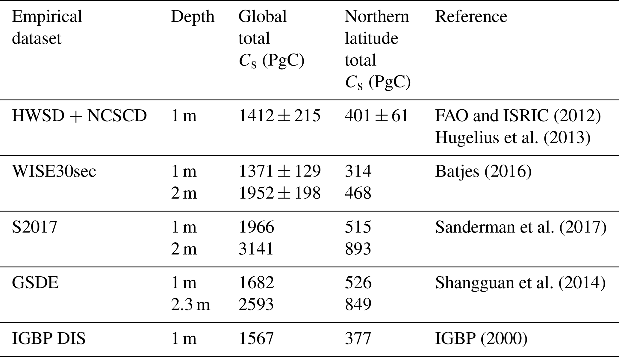
Moreover, additional empirical datasets are considered to improve the reliability of the benchmark dataset (Table 3). These additional datasets include the following: (1) the World Inventory of Soil property Estimates (WISE30sec) dataset down to a depth of 2 m (Batjes, 2016), which includes a given standard deviation on the global total soil carbon consistent with our derived benchmark uncertainty, (2) the named “S2017” from the Sanderman et al. (2017) soil carbon estimate (1 and 2 m), which uses a data-driven statistical model and the History Database of the Global Environment (HYDE) land use data, (3) the Global Soil Dataset for use in Earth system models (GSDE), which provides estimates for observational soil carbon down to a depth of up to 2.3 m (Shangguan et al., 2014), and (4) the Global Gridded Surfaces of Selected Soil Characteristics (IGBP-DIS) estimate of soil carbon to a depth of 1 m, derived by the Oak Ridge National Laboratory Distributed Active Archive Centre (ORNL DAAC) (IGBP, 2000). These datasets were combined to obtain a mean estimate for observational soil carbon down to a depth of 1 m, where a global total soil carbon value of 1560 ± 214 PgC was found. This estimate is consistent with our benchmark dataset estimate and further improves the confidence in our benchmark dataset.
Furthermore, the spatial correlation coefficients between these additional datasets and our benchmark dataset are considered, where the following values correspond to the above datasets: (1) 0.554, (2) 0.625, (3) 0.482, and (4) 0.622. Map plots comparing the empirical soil carbon datasets are shown in Fig. A1. The estimate for northern latitude total soil carbon has greater uncertainties associated with it, where the standard deviation deduced by combining the empirical datasets is ± 83 PgC. To account for this increased uncertainty in these regions, the deduced standard deviation of ± 83 PgC is used on the benchmark soil carbon throughout this study, as opposed to the ± 61 PgC derived using the Todd-Brown et al. (2013) uncertainty analysis.
2.3.2 Carbon fluxes
To estimate a benchmark NPP, the commonly used MODIS NPP (2000–2010) dataset (Zhao et al., 2005) is used. The MODIS NPP dataset does not have associated uncertainty estimates, so this study estimates a standard deviation error on the benchmark NPP as derived by Ito (2011). The MODIS NPP dataset is found to be consistent with 251 empirical present-day estimates of NPP found in the literature, which Ito (2011) used to estimate a global value of 56.2 ± 14.3 PgC yr−1 (compared with a derived MODIS mean value of 56.6 yr−1).
Moreover, due to the limited choice of observationally derived NPP datasets (Harper et al., 2018), models can be further evaluated using a benchmark dataset for Rh, where Rh is estimated using the CARDAMOM (2001–2010) heterotrophic respiration dataset (Bloom et al., 2015). The empirical CARDAMOM Rh has associated estimates of error, which were used to derive a standard deviation uncertainty on the empirical average Rh (51.7 ± 21.8 PgC yr−1). This study includes map plots comparing the two empirical datasets, which is shown in Fig. A2. Global totals for Rh are also considered for comparison against NPP, where the CMIP6 and CMIP5 values are also shown in Appendix Tables A1 and A2, respectively.
2.3.3 Soil carbon turnover time
To estimate a benchmark τs, the estimates of observational Cs are divided by an estimate of Rh (see Eq. 1). To estimate an uncertainty on the effective global τs, this study derived upper () and lower () bounds based on the derived Cs and Rh uncertainty estimates. The upper bound was calculated using the following: / , where is equal to the mean soil carbon plus 1 standard deviation and is equal to the mean heterotrophic respiration minus 1 standard deviation. The lower bound was calculated using the following: / , where similarly is equal to the mean soil carbon minus 1 standard deviation and is equal to the mean heterotrophic respiration plus 1 standard deviation.
This method gives a large uncertainty bound around the derived mean estimate (27.0 years), so the benchmark data are further compared with empirical estimates. Raich and Schlesinger (1992) derived an estimate of mean soil carbon turnover of 32 years, using estimates for mean soil carbon pools and mean soil respiration rates. More recently, Carvalhais et al. (2014) derived an estimate for the mean global ecosystem carbon turnover time of 23 years, which is a spatially explicit and observation-based estimate. Ito et al. (2020) derived an observational uncertainty range on soil carbon turnover time of 18.5 to 45.8 years, which was derived using similar empirical estimates found in the literature. These estimates give more certainty on the values closer to the derived empirical mean value for τs.
2.3.4 Soil moisture and air temperature
To estimate soil moisture (θ), the Copernicus Climate Change Service (C3S) “Soil moisture gridded data from 1978 to present” dataset (published 25 October 2018) is used, where the years 1978 to 2000 are considered. This dataset is based on the ESA Climate Change Initiative soil moisture and estimates global surface soil moisture from a large set of satellite sensors (Copernicus Climate Change Service, 2021; Liu et al., 2011, 2012; Wagner et al., 2012; Gruber et al., 2017; Dorigo et al., 2017). The WFDEI meteorological forcing dataset is used to represent observational air temperatures (1995–2005) (Weedon et al., 2014), where dates are chosen to allow for consistency between CMIP generations. This study includes no uncertainty analysis of the soil moisture and air temperature empirical datasets as these datasets are only used to evaluate spatial correlations between variables and not to evaluate soil moisture and air temperature in the models.
2.4 Regridding
To allow direct comparisons between the empirical data and model output data, the model data were regridded to match the observational grid. In this case, the observational grid is a 0.5∘ by 0.5∘ resolution, 720 longitude and 360 latitude grid. The regridding was done using Iris – the community-driven Python package for analysing and visualising Earth science data (Met Office, 2010–2013). The regridding method assumed conservation of mass and used linear extrapolation, where extrapolation points will be calculated by extending the gradient of the closest two points. Moreover, model land masks are used to calculate the fraction of land in each coastal grid cell (CMIP variable sftlf).
2.5 Statistical analysis
It is difficult to evaluate the spatial distributions of modelled soil carbon and related spatial controls against empirical data with a single metric, so the evaluation for both CMIP6 and CMIP5 involves multiple methods. These include coefficients of variation, spatial standard deviations, spatial Pearson correlation coefficients, and root mean square errors (RMSEs). These methods can be combined to give a more thorough evaluation of spatial soil carbon and associated controls in the CMIP6 models compared with the previous generation of CMIP5 models.
The coefficient of variation is defined as the ratio of the ensemble standard deviation (SD) to the ensemble mean in each grid cell. This is used to show the amount of variability amongst the models in the ensemble scaled to the size of the ensemble mean and so represents the variability spatially in the ensemble and shows how much variation is present across the ensemble in specific regions. It is presented as hatching in a map figure (Fig. 3), where shaded “hatched” regions show regions of high variability within the ensemble. These regions show areas where there is disagreement in the ensemble as there is a large spread compared with the mean and was defined as being where SD mean >0.75. The regions where spatial Cs<5 kg m−2 were discounted as low values of soil carbon are present in these regions.
The spatial standard deviation is a measure of the spread in the data across the globe compared with the mean value. Pearson correlation coefficients (r values) were used as a spatial measure of the linear correlation between the empirical and modelled data, where a high r value (near 1 or −1) represents a high correlation in the data and a low r value (near 0) represents a negligible correlation. RMSEs were used as an absolute measure of the difference between the modelled and empirical data, where the lower the value, the lower the difference error. The RMSE can be considered as the standard deviation of the difference, and it is a measure to show the deviation of the modelled data in relation to the empirical data. These statistical data, spatial standard deviations, Pearson correlation coefficients, and RMSEs can be presented using a Taylor diagram. A Taylor diagram is a graph used to indicate the performance of a model compared with a benchmark, which in this case are the empirical datasets (Taylor, 2001).
3.1 Soil carbon stocks: northern latitude underestimations remain in CMIP6
3.1.1 Global total evaluation
Global total soil carbon (in the top 1 m of soil) is shown to vary amongst the ESMs in CMIP6, with a range of 1294 PgC between the models with the lowest and highest values (Table 4). The global total soil carbon for 2 (CanESM5 and MIROC-ES2L) out of the 11 CMIP6 models falls within the benchmark soil carbon uncertainty range, 1197–1627 PgC (mean ± stand deviation). The models with the largest global total soil carbon are CNRM-ESM2-1 (1810 PgC), BCC-CSM2-MR (1770 PgC), and UKESM1-0-LL (1760 PgC), values greater than the benchmark dataset but not the additional empirical datasets (Table 3). The models GFDL-ESM4 (516 PgC) and IPSL-CM6A-LR (639 PgC) have the lowest global total soil carbon values in the ensemble, with global totals significantly lower (approximately 50 % less) than the global totals seen in empirical data. It is noted that, if the full soil carbon profile is considered for CESM2 and NorESM2-LM opposed to a depth of 1 m, the global total soil carbon values are increased to 1870 PgC from 991 PgC in CESM2 and to 2430 PgC from 969 PgC in NorESM2-LM.
Table 4Table presenting global soil carbon values for the 11 CMIP6 models included in this study and the benchmark datasets, including global total Cs in PgC, northern latitude total (90–60∘ N) Cs in PgC, and the spatial mean value of Cs with the corresponding standard deviation in kg m−2.
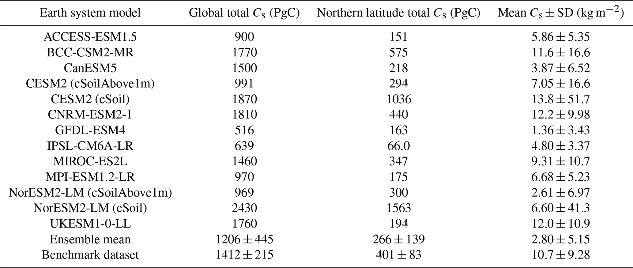
Both the CMIP5 and CMIP6 ensemble mean global totals fall within the benchmark uncertainty range (Tables 4 and 5). The ensemble mean global total soil carbon is found to have decreased in CMIP6 from CMIP5 (1206 ± 445 PgC vs. 1480 ± 810 PgC). However, a significant reduction is seen in the associated standard deviation of the ensemble mean global totals in CMIP6 compared with CMIP5 (± 445 PgC in CMIP6 from ± 810 PgC in CMIP5) and a reduced range of global total values (a range of 1294 PgC is seen in CMIP6 as opposed to 2493 PgC in CMIP5). This suggests that, although a significant range in global soil carbon still exists amongst the CMIP6 ESMs, there is an improved consistency between the models seen in CMIP6 compared with the models in CMIP5, although it is noted that this may be a factor of the selection of models included in each ensemble rather than any change in process representation.
Table 5Table presenting global soil carbon values for the 10 CMIP5 models included in this study and the benchmark datasets, including global total Cs in PgC, northern latitude total (90–60∘ N) Cs in PgC, and the spatial mean value of Cs with the corresponding standard deviation in kg m−2.
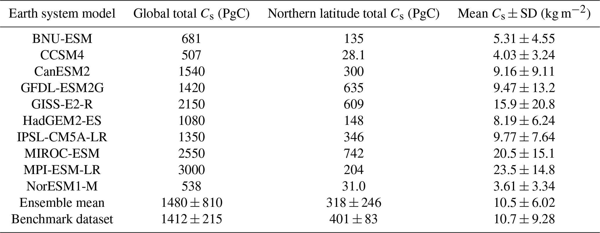
It is found from comparing the previous-generation models in CMIP5 with the updated CMIP6 equivalent that multiple models in CMIP6 have lower quantities of soil carbon than in CMIP5, such as GFDL-ESM4 from GFDL-ESM2G, IPSL-CM6A-LR from IPSL-CM5A-LR, MIROC-ES2L from MIRCO-ESM, and MPI-ESM1.2-LR from MPI-ESM-LR. For example, the CMIP5 model MPI-ESM-LR is reported to have the largest soil carbon magnitude amongst the CMIP5 models, with a global total of 3000 PgC (Table 5), whereas the updated CMIP6 model MPI-ESM1.2-LR has a reduced global total soil carbon value of 970 PgC amongst the lowest values reported in CMIP6 and below the observationally derived range (Table 4). Conversely, these reductions are negated in the ensemble mean by the remaining models, which have greater quantities of soil carbon in CMIP6 compared with their CMIP5 equivalent, such as CanESM5 from CanESM2, CESM2 from CCSM4, NorESM2-LM from NorESM1-M, and UKESM1-0-LL from HadGEM2-ES. For example, the CMIP5 model NorESM1-M is amongst the lowest soil carbon values presented in this ensemble at 538 PgC (Table 5), whereas the updated CMIP6 model NorESM2-LM has an increased global total of 969 PgC (down to 1 m) (Table 4).
3.1.2 Northern latitude total evaluation
Northern latitude soil carbon (down to a depth of 1 m and where northern latitudes are defined as 60–90∘ N) is found to be underestimated in CMIP6, with 8 out of the 11 CMIP6 models having lower northern latitude soil carbon values than the derived observational range (Table 4). A total of 2 of the 11 CMIP6 models (CNRM-ESM2-1 and MIROC-ES2L) have northern latitude totals that fall within the uncertainty range derived from the benchmark data, 318–484 PgC (mean ± stand deviation). The CMIP6 models with the greatest northern latitude total soil carbon are BCC-CSM2-MR (575 PgC), CNRM-ESM2-1 (440 PgC), and MIROC-ES2L (347 PgC). The CMIP6 models with the lowest northern latitude soil carbon are IPSL-CM6A-LR (66 PgC), ACCESS-ESM1.5 (151 PgC), GFDL-ESM4 (163 PgC), MPI-ESM1.2-LR (175 PgC), and UKESM1-0-LL (194 PgC), values significantly lower than the totals seen in empirical data.
The northern latitude soil carbon total was also underestimated in CMIP5, with 6 out of the 10 CMIP5 models estimating northern latitude totals lower than the empirical estimates (Table 5). The ensemble mean total northern latitude soil carbon is lower in CMIP6 (266 ± 139 PgC seen in Table 4) than in CMIP5 (318 ± 246 PgC seen in Table 5), which is consistent with the global total results; however, both the CMIP5 and CMIP6 mean values fall below the benchmark range. Similarly, as with global soil carbon, a smaller standard deviation on the mean is found for CMIP6 compared with CMIP5, and there is a reduced range in simulated northern latitude total values amongst the CMIP6 models, where despite a large range seen (66 to 575 PgC), an even greater range is seen in CMIP5 (28.1 to 742 PgC). Moreover, improvements are seen amongst models from CMIP5 to CMIP6. For example, the CMIP5 model NorESM1-M had a northern latitude total soil carbon value of 31.0 PgC, which is significantly lower than what is expected based on the benchmark dataset (Table 5). However, the updated CMIP6 version of this model, NorESM2-LM, has a northern latitude total soil carbon value of 300 PgC, which is much more in line with the expected observational values (Table 4). An improved representation of northern latitude soil carbon is also seen in CESM2 (compared with CCSM4), which has the same land surface model as NorESM2-LM (CLM5 Lawrence et al., 2019).
The CMIP6 models with the lowest global total values for soil carbon do not always correspond to the lowest northern latitude values for soil carbon. For example, UKESM1-0-LL global total soil carbon is amongst the highest global totals seen in CMIP6; however, low quantities of soil carbon are seen in the northern latitudes (approximately 10 % of the global total). Conversely, BCC-CSM2-MR, CESM2, GFDL-ESM4, and NorESM2-LM have approximately 30 % of their global total stocks in the northern latitude region, which is consistent with the ratio seen in the benchmark dataset. This result suggests that representing global total soil carbon stocks consistently with the benchmark soil carbon does not imply consistency in the representation of northern latitude soil carbon stocks, and these should be evaluated separately. However, the large uncertainties associated with the empirical datasets for the northern latitudes are noted (Table 3).
3.1.3 Spatial evaluation
A lack of consistency in the simulation of soil carbon was found amongst the CMIP5 models, which can be seen in Fig. 1a, where differences between the empirical and modelled data are shown. Northern latitude soil carbon was found to be underestimated in CMIP5, where areas of blue can be seen in the northern latitudes of the CMIP5 soil carbon map in Fig. 1a. This underestimation of CMIP5 northern latitude soil carbon is accompanied by significant overestimations seen in mid-latitude soil carbon. Specifically, large quantities of soil carbon which are inconsistent with our benchmark dataset can be seen in the mid-latitude regions in the following CMIP5 models: CanESM2, GFDL-ESM2G, GISS-E2-R, MIROC-ESM, and MPI-ESM-LR. Less significant overestimations are seen in HadGEM2-ES and IPSL-CM5A-LR (Fig. A3). Systematic errors remain in the CMIP6 models; however, there are some improvements seen in the spatial simulation of soil carbon from CMIP5. Soil carbon is still underestimated in the northern latitudes, where the areas of blue still remain in the northern latitudes of the CMIP6 soil carbon map in Fig. 1a, though regions of overestimations in the northern latitudes are also seen amongst the CMIP6 models in BCC-CSM2-MR, CESM2, CNRM-ESM2-1, and NorESM2-LM (Fig. 2), but it is noted that this representation might be more consistent with observations if a dataset including deeper soil carbon stocks was considered. CMIP6 shows improvements in the representation of mid-latitude soil carbon, where less of an overestimation is seen in CMIP6 compared with CMIP5 (Fig. 1a). This overestimation can still be seen in 4 of the 11 CMIP6 models: ACCESS-ESM1.5, CanESM2, MIROC-ES2L, and UKESM1-0-LL; however, the overestimations in CMIP6 are less inconsistent than when compared with CMIP5, and the number of models showing this limitation in CMIP6 has been reduced (Fig. 2).
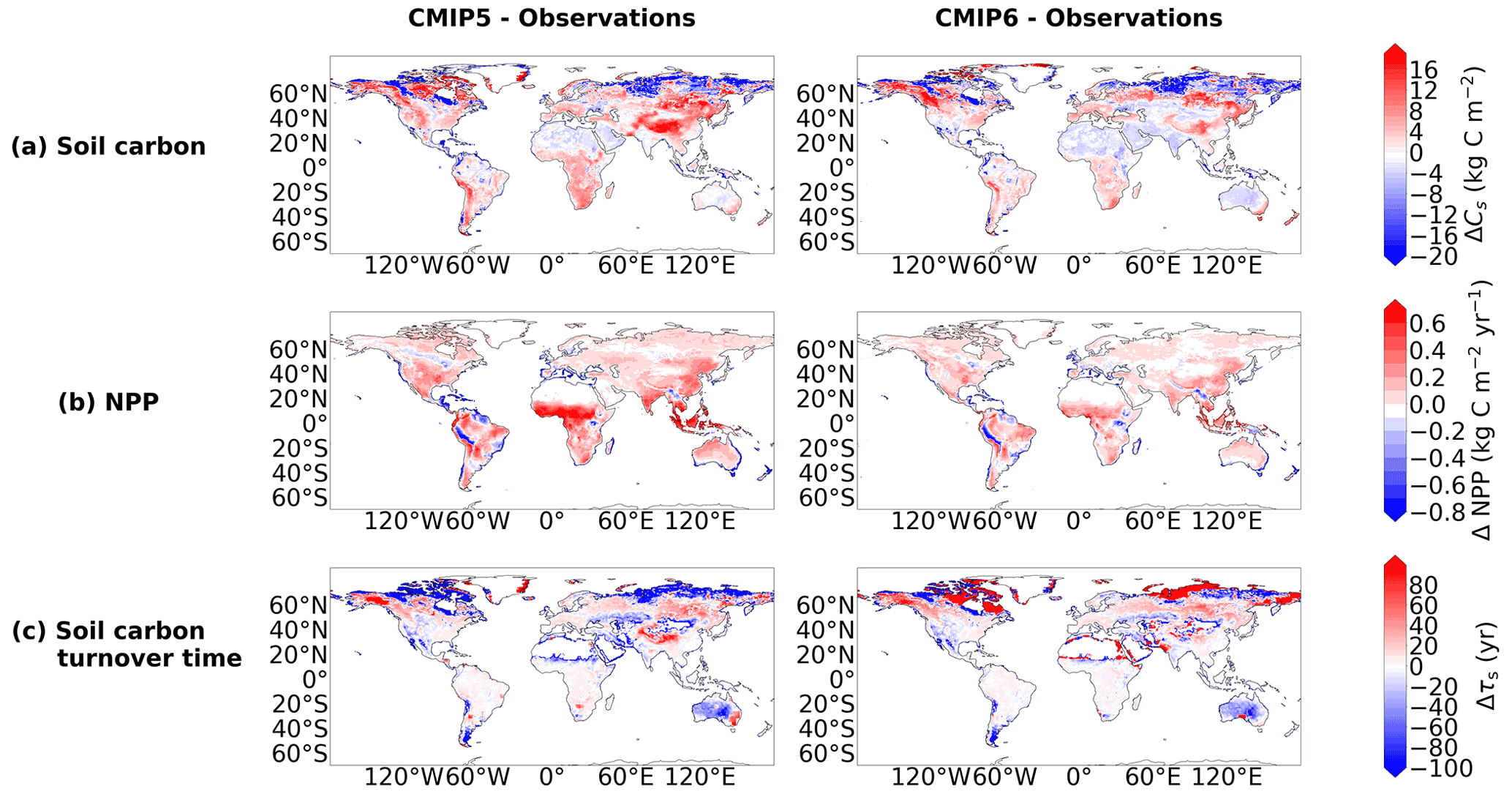
Figure 1Maps presenting the difference between the modelled and benchmark data for the CMIP5 and CMIP6 ensembles, for (a) Cs (kg m−2), (b) NPP (kg m−2 yr−1), and (c) τs (years).

Figure 2Maps of the difference in soil carbon (Cs) between the historical simulation of each CMIP6 model and the benchmark data.
Despite the differences seen in the spatial representation of soil carbon between the individual models in CMIP6, the ensemble mean has more areas of agreement within the ensemble compared with the ensemble mean in CMIP5. This can be seen in Fig. 3a, where there is less hatching (where hatched shaded areas represent regions of low agreement amongst the models in the ensemble; see Methods) in the CMIP6 map compared with the CMIP5 map. Specifically, ensemble mean soil carbon in CMIP6 has more areas of agreement in the mid-latitude region compared with the CMIP5 ensemble mean, where significant areas of disagreement are seen. This disagreement is likely due to the overestimation which exists in some of the CMIP5 models (Fig. A3). Also, a reduction in the area of disagreement is seen in the northern latitudes in CMIP6 compared with CMIP5; however, this remains the region where the most disagreement exists across the generations. It is noted that this is a measure of agreement within the ensemble and not between the models and empirical data and so is dependent on the choice of ensemble members (see Figs. A6 and A7 for individual model maps).

Figure 3Ensemble mean maps for (a) Cs (kg m−2), (b) NPP (kg m−2 yr−1), and (c) τs (years), presented for the CMIP6 ensemble, the CMIP5 ensemble, and the benchmark datasets. The hatched areas are used to show regions of low agreement within the ensemble (SD / mean >0.75) and where regions of low soil carbon (< 5 kg m−2) have been excluded. Equivalent maps for the individual CMIP6 and CMIP5 models are shown within the Appendix: see Figs. A6 and A7 for Cs, Figs. A8 and A9 for NPP, and Figs. A10 and A11 for τs, respectively.
The inconsistency of the simulation of spatial soil carbon in CMIP6 is further evaluated using the spatial standard deviations, the spatial Pearson correlation coefficients, and RMSEs (see Methods), where the Taylor diagram (Fig. 4a) presents all three statistical assessments. The spatial standard deviation for soil carbon is shown on the radial axis between the standard x and y axes in Fig. 4a. The range of spatial standard deviations amongst the CMIP6 models sees a slight reduction from the range amongst the CMIP5 models, though significant differences remain. The CMIP6 models CNRM-ESM2-1, MIROC-ES2L, and UKESM1-0-LL best match the spatial standard deviation derived from the benchmark dataset (Tables 4 and 5). It is found that the spatial representation of modelled soil carbon in CMIP6 is poorly correlated with the empirical soil carbon, where the CMIP6 ensemble spatial correlation coefficient with the empirical data is found to be 0.250. The spatial correlation coefficients between the individual CMIP6 and CMIP5 models with the empirical data can also be seen in Fig. 4a, where the low spatial correlation coefficients are shown by the curved correlation axis. The lowest spatial correlation coefficients amongst the CMIP6 models were r values of 0.104 in IPSL-CM6A-LR and 0.115 in UKESM1-0-LL. The CMIP6 model that was the most spatially consistent with the empirical data is CNRM-ESM2-1, with an r value of 0.630. The CMIP6 ensemble sees a slight reduction in the RMSE compared with the CMIP5 ensemble, suggesting a slight improvement (Fig. 5a). Significant improvements in the RMSE are seen in MIROC-ES2L from MIROC-ESM and MPI-ESM1.2-LR from MPI-ESM-LR. These results suggest small improvements in the simulation of soil carbon across this CMIP generation; however, the low spatial correlation coefficients and variable RMSEs seen across the models in CMIP6 suggest that inconsistencies with the benchmark data remain.
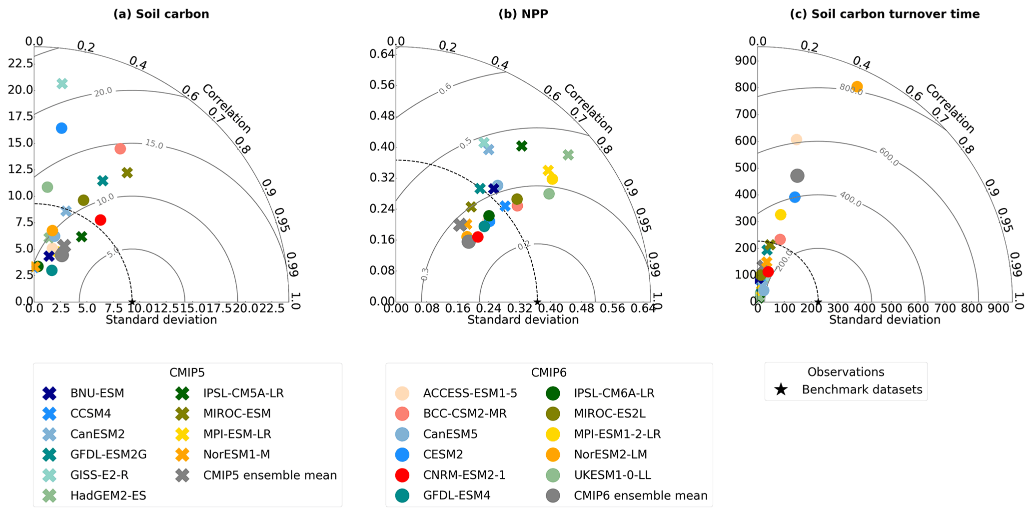
Figure 4Taylor diagrams showing the spatial standard deviation (shown by the radial axis between standard x and y axes), the Pearson correlation coefficients (shown by the curved correlation axis), and the RMSE (shown by the grey contours) for the ESMs in both CMIP5 and CMIP6 compared with the benchmark datasets, for (a) soil carbon (Cs), (b) NPP, and (c) soil carbon turnover time (τs).
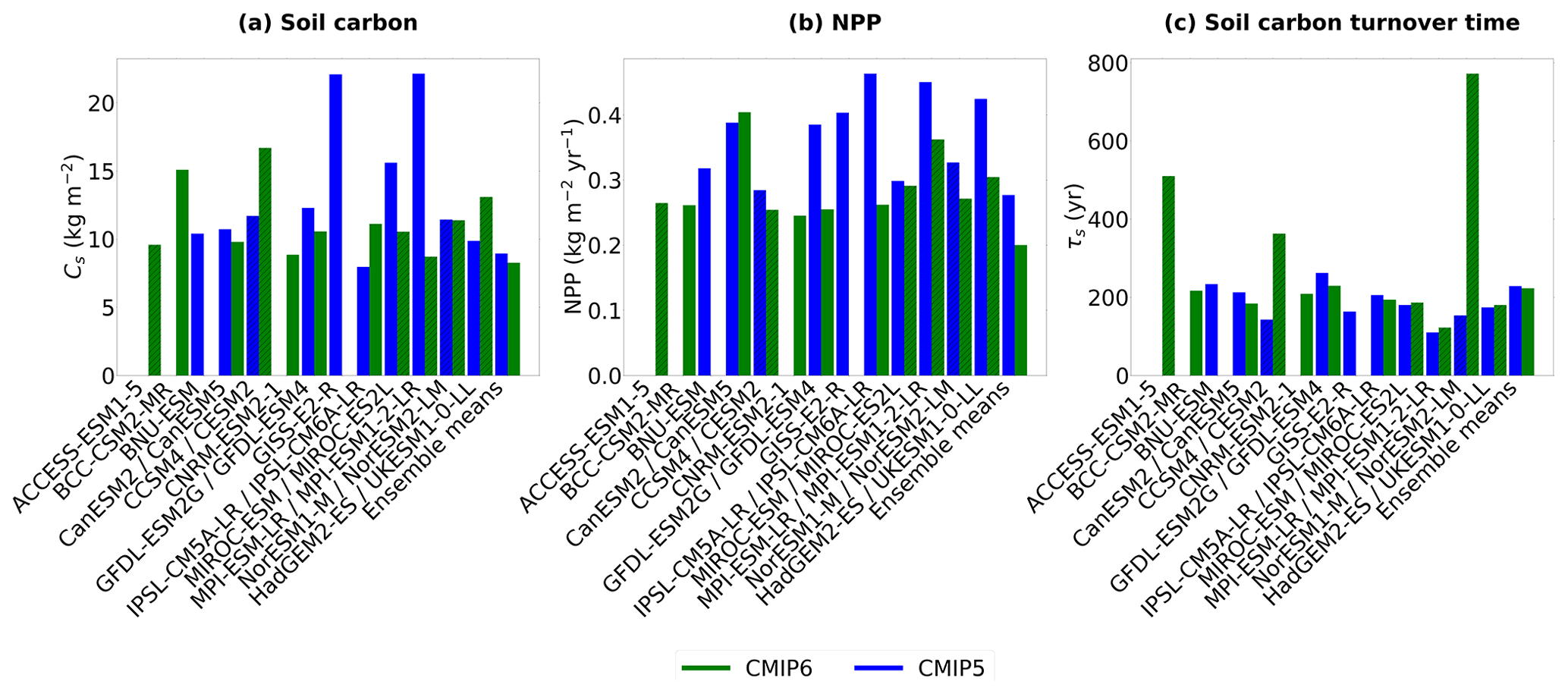
Figure 5Bar charts comparing the root mean squared errors (RMSEs) in CMIP6 and CMIP5 for (a) soil carbon (Cs), (b) NPP, and (c) soil carbon turnover time (τs).
3.2 Net primary productivity: improved in CMIP6 relative to CMIP5
3.2.1 Global total evaluation
Global total NPP amongst the CMIP6 models appears to be consistent with the benchmark dataset (Table 6), where the CMIP6 ensemble mean for NPP is approximately 95 % of the benchmark mean. The CMIP6 ensemble mean global total NPP (53.0 ± 9.39 PgC yr−1) is found to be slightly lower than the derived mean benchmark value; however, it is comfortably within the observational uncertainty range (56.6 ± 14.3 PgC yr−1). The equivalent values for the CMIP5 models can be seen in Table 7, where the CMIP5 ensemble total is also found to be within the observational uncertainty range (56.3 ± 15.4 PgC yr−1).
Table 6Table presenting global carbon fluxes and turnover time values for the 11 CMIP6 models included in this study and the benchmark datasets, including global total NPP (PgC yr−1) and the effective average soil carbon turnover time (years).
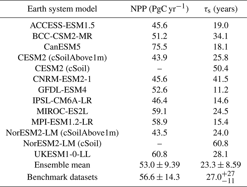
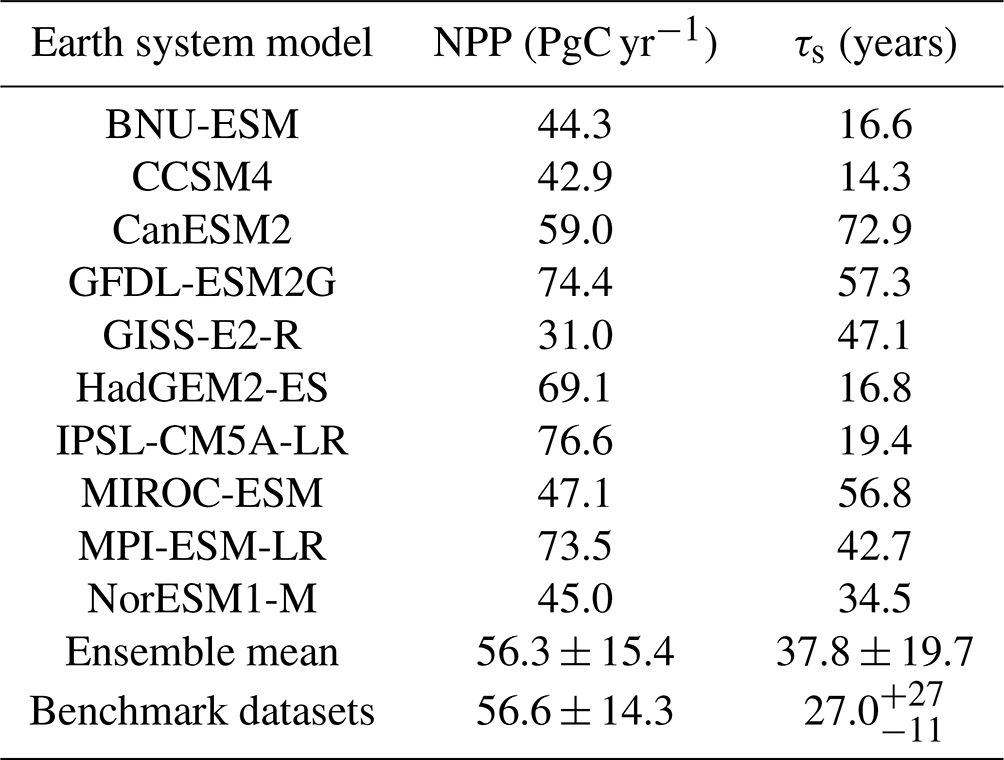
Table 7Table presenting global carbon fluxes and turnover time values for the 10 CMIP5 models included in this study and the benchmark datasets, including global total NPP (PgC yr−1) and the effective average soil carbon turnover time (years).
The standard deviation surrounding the CMIP5 ensemble mean is greater than in CMIP6. This reduced standard deviation in CMIP6 is because several of the models have a simulated global total NPP that more closely matches the benchmark NPP global total value compared with the previous CMIP5 generation: GFDL-ESM4 from GFDL-ESM2G, IPSL-CM6A-LR from IPSL-CM5A-LR, MIROC-ES2L from MIROC-ESM, MPI-ESM1.2-LR from MPI-ESM1-M, and UKESM1-0-LL from HadGEM2-ES. The majority of CMIP6 models see a reduction in NPP from the CMIP5 equivalent model, which in general reduces the overestimation of NPP that was seen in the CMIP5 models (Tables 6 and 7). However, this was not the case for CanESM5 from CanESM2, which sees an increase in the magnitude of NPP from CMIP5 to CMIP6, resulting in a consequent overestimation compared with the benchmark data. A reduced range of modelled global total NPP values is also seen in CMIP6 from CMIP5, where the range is reduced from 48.5 PgC yr−1 in CMIP5 to 32.7 PgC yr−1 in CMIP6. These results suggest that, overall, the representation of carbon fluxes in CMIP6 ESMs is more consistent than in CMIP5.
3.2.2 Spatial evaluation
Modelled NPP in CMIP6 appears to be spatially more consistent with the empirical data than in CMIP5. This is suggested by Fig. 1b, where the difference between the modelled and benchmark NPP is shown for both CMIP5 and CMIP6. It can be seen in the CMIP5 map that NPP is overestimated in the tropical regions, specifically in Africa and South-East Asia, and the equivalent CMIP6 difference map shows a clear reduction in this overestimation. This tropical overestimation of NPP, prominent in CMIP5 (Fig. A4), is still seen in the CMIP6 models: CanESM5, MPI-ESM1.2-LR, and UKESM1-0-LL. However, this is not seen in the CMIP6 ensemble mean as it is likely negated by underestimations seen in CESM2, CNRM-ESM2-1, and NorESM2-LM (Fig. 6). CMIP6 also sees more consistency with the benchmark dataset in the northern and mid-latitude regions compared with CMIP5, where more white areas are seen in the CMIP6 map in Fig. 1b. An underestimation of NPP is seen in both CMIP5 and CMIP6 on the western side of South America, though unusually high NPP is seen in this region in the MODIS NPP dataset (Fig. A2). Moreover, greater agreement amongst the models within CMIP6 is seen compared with the models in CMIP5. This can be seen in Fig. 3b, where less hatching representing areas of disagreement within the ensemble is seen in CMIP6 compared with CMIP5. Specifically, CMIP6 sees less hatching in the northern latitudes and in the Middle East and south-eastern Europe as well as regions in South America, southern Africa, and Australia (see Figs. A8 and A9 for individual model maps).
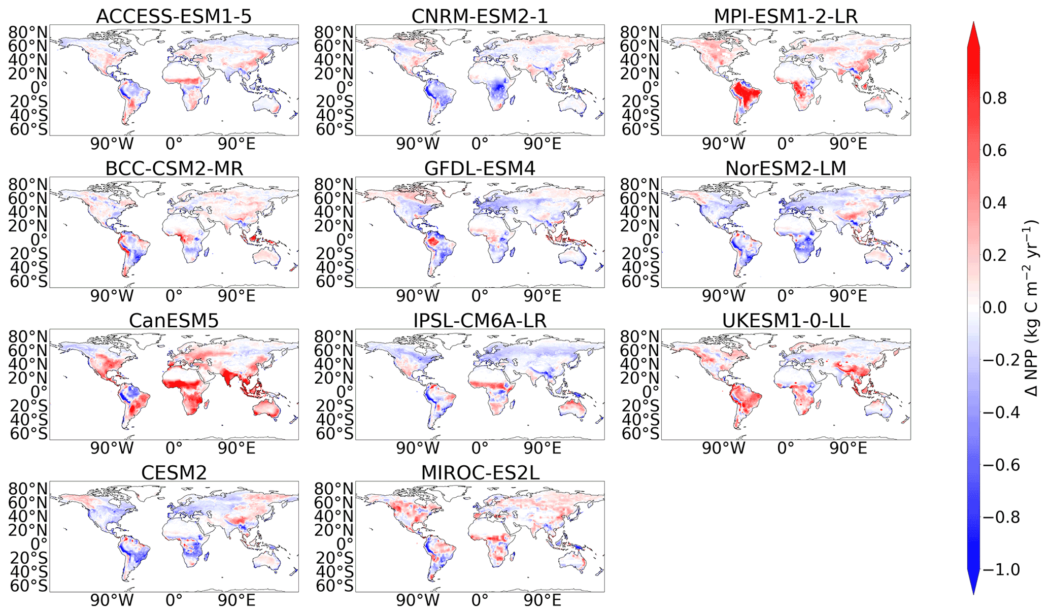
Figure 6Maps of the difference in net primary production (NPP) between the historical simulation of each CMIP6 model and the benchmark dataset.
The improved empirical consistency of modelled NPP in CMIP6 is also suggested when further evaluated using the same spatial metrics as with soil carbon. Despite a small range remaining in the spatial standard deviations amongst the CMIP6 models (shown by the radial axis in Fig. 4b), robust improvements in the spatial correlation coefficients (shown by the curved axis in Fig. 4b) and RMSEs are seen across the ensemble compared with CMIP5 (Fig. 5b). Notable improvements in the representation of NPP are seen in GFDL-ESM4 compared with GFDL-ESM2G, IPSL-CM6A-LR compared with IPSL-CM5A-LR, and UKESM1-0-LL compared with HadGEM2-ES, with reduced RMSEs seen in each updated model. A general improvement in the spatial correlation coefficients is seen across all the CMIP6 models, where the circle markers (CMIP6 models) in Fig. 4b have higher correlation values than the cross markers (CMIP5 models). The general improvement has resulted in the CMIP6 ensemble correlation coefficient (0.836) being greater compared with the equivalent CMIP5 value (0.711). The lowest correlations between modelled and observed NPP amongst the CMIP5 models are GISS-E2-R (0.274) and CanESM2 (0.469). The updated version CanESM5 remains the lowest correlation seen in CMIP6 (0.655); however, an improvement in the correlation is seen. The updated version of the GISS model is not included in the CMIP6 ensemble considered in this study, which could be a reason for the increased ensemble mean correlation. However, this effect does not take away from the improvements seen across the CMIP6 models. HadGEM2-ES (0.764) and MPI-ESM-LR (0.764) were the CMIP5 models with the highest correlation with the benchmark NPP, and the updated CMIP6 equivalents of these models remain the models with the greatest correlations, but again improvements in the correlations are seen (0.816 in UKESM1-0-LL and 0.785 in MPI-ESM1.2-LR).
3.3 Soil carbon turnover time: no major improvements in CMIP6 compared with CMIP5
3.3.1 Global evaluation
There are minor improvements suggested in the simulated effective global τs amongst select CMIP6 models (Table 6) compared with CMIP5 (Table 7). The ensemble mean effective global τs was overestimated in CMIP5 (37.8 ± 19.7 years) when compared with the derived mean τs using the benchmark datasets (27.0 years), which is reduced to a less significant underestimation in CMIP6 (23.3 ± 8.59 years), though both the CMIP5 and CMIP6 estimates fall within the observational uncertainty range. The associated ensemble spread in effective mean τs is less in CMIP6 compared with CMIP5, with an ensemble standard deviation of approximately 50 % less. A significant range is seen in the effective global τs values amongst the CMIP5 models, with a 5-fold difference between the lowest and highest values (Table 7). This range is mostly due to large overestimations seen amongst the CMIP5 models, for example in CanESM2, GFDL-ESM2G, and MIROC-ESM. A reduced range is seen amongst the models in CMIP6; however, a 4-fold range still exists between the lowest and highest values (Table 6). This reduced range is partly due to reductions in the effective global τs values in CMIP6 models compared with the equivalent model in CMIP5, specifically, CanESM5 from CanESM2, GFDL-ESM4 from GFDL-ESM2G, MIROC-ES2L from MIROC-ESM, and MPI-ESM1.2-LR from MPI-ESM-LR, though overestimations do remain in CMIP6, for example in CNRM-ESM2-1, where the slowest effective turnover time was seen. Moreover, the range is also reduced due to improvements seen in models which underestimated τs in CMIP5, such as UKESM1-0-LL from HadGEM2-ES and CESM2 from CCSM4.
3.3.2 Spatial evaluation
The comparison of spatial τs in CMIP6 with CMIP5 has more varied results compared with simulated NPP. The CMIP5 ensemble showed an underestimation of τs in the northern latitudes, which is replaced with an overestimation of τs in CMIP6 when compared with the benchmark data (Fig. 1c). This northern latitude overestimation in the CMIP6 ensemble is a result of the overestimations of τs in CESM2 and NorESM2-LM (Fig. 7), which dominate in the CMIP6 ensemble mean. It is noted that this result may differ if deeper soil carbon stocks were considered. The northern latitude underestimation of τs is still seen within the CMIP6 models: CanESM5, CNRM-ESM2-1, GFDL-ESM4, IPSL-CM6A-LR, MIROC-ES2L, MPI-ESM1.2-LR, and UKESM1-0-LL (Fig. 7). An overestimation of mid-latitude τs was seen in the CMIP5 models MIROC-ESM and MPI-ESM-LR (Fig. A5), which is no longer seen in the equivalent updated CMIP6 models MIROC-ES2L and MPI-ESM1-2-LR. However, an overestimation of mid-latitude τs is seen in CMIP6 models BCC-CSM2-MR, CNRM-ESM2-1, and UKESM1-0-LL (Fig. 7). The uncertainty in simulated northern latitude τs is also apparent in Fig. 3c, where the hatching shows the lack of agreement within the CMIP6 ensemble in this region. However, more agreement within the CMIP6 ensemble is seen in the same figure in the mid-latitudes and in the tropical regions compared with CMIP5 (see Figs. A10 and A11 for individual model maps).
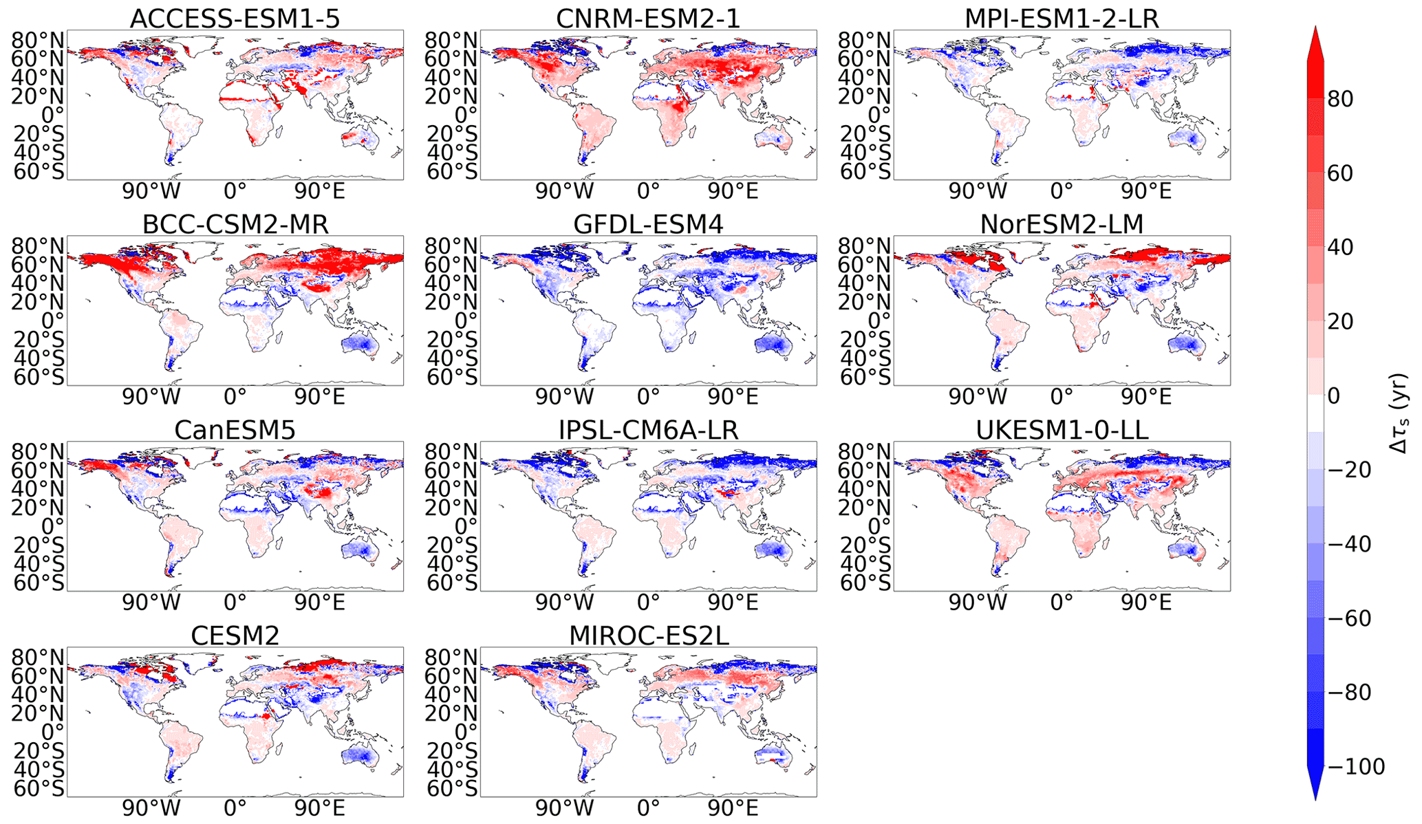
Figure 7Maps of the difference in soil carbon turnover time (τs) between the historical simulation of each CMIP6 model and the benchmark datasets.
The simulation of spatial τs in CMIP6 is further evaluated against the empirical data with the additional statistical metrics. Modelled τs is found to be poorly spatially correlated with empirical τs in both the CMIP5 and CMIP6 models (shown by the curved axis in Fig. 4c). A slight increase in the ensemble mean spatial correlations is seen from CMIP5 (0.188) to CMIP6 (0.267) due to increases seen amongst individual models between CMIP5 and CMIP6: CESM2 from CCSM4, MPI-ESM1.2-LR from MPI-ESM-LR, and NorESM2-LM from NorESM1-M. However, the consistency of modelled τs with the benchmark datasets remains low. A particularly large range is seen in the spatial standard deviations of τs amongst the CMIP6 models, which is an increased range from CMIP5 (shown by the radial axis in Fig. 4c). The CMIP6 models with the most extreme overestimations of the spatial standard deviations compared with the derived benchmark value (NorESM2-LM, CESM2, and ACCESS-ESM1.5) are also found to have large RMSEs (Fig. 5c). Amongst the remaining CMIP6 models, the RMSEs for modelled τs remain relatively consistent between CMIP5 and CMIP6.
3.4 Drivers of soil carbon spatial patterns: soil carbon spuriously highly correlated with NPP in CMIP5 and CMIP6
3.4.1 Global drivers
A negligible correlation (≈ 0) is found between the benchmark estimates of soil carbon and NPP, suggesting that soil carbon is not spatially correlated with NPP in the real world. On the other hand, soil carbon and NPP (Cs–NPP) were found to be significantly correlated in the models in both CMIP5 and CMIP6. The Cs–NPP spatial correlation was found to be greater than 0.5 for 6 out of the 10 CMIP5 ESMs and 8 out of the 11 models in CMIP6 (Fig. 8a). However, a low spatial correlation is found in the CMIP6 models CESM2 (0.134), NorESM2-LM (0.261), and BCC-CSM2-MR (0.214), values most consistent with the benchmark datasets. The Cs–τs spatial correlations found in the CMIP6 models tend to underestimate the positive correlation seen in the benchmark datasets (Fig. 8a). The majority of CMIP6 models see a negligible or slightly negative Cs–τs spatial correlation despite a low positive correlation produced by the benchmark datasets. The models BCC-CSM2-MR, MIROC-ES2L, and NorESM2-LM are most consistent with the benchmark Cs–τs correlation.
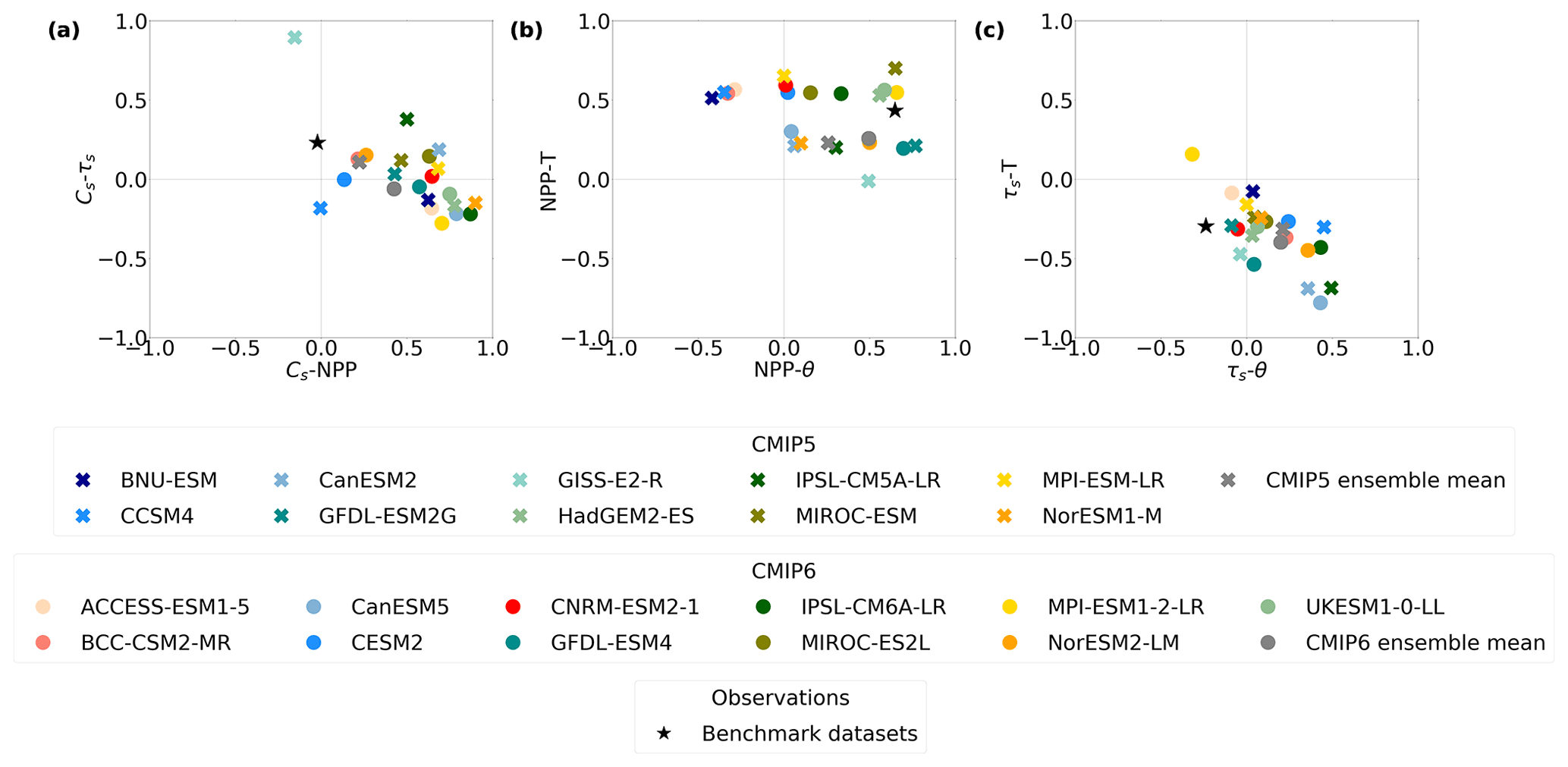
Figure 8Scatter plots investigating the relationships between different Pearson correlation coefficients of climate variables, (a) Cs–τs against Cs–NPP, (b) NPP–T against NPP–θ, and (c) τs–T against τs–θ.
The modelled NPP to temperature (NPP–T) spatial correlations in CMIP6 are consistent with the positive relationship seen in the benchmark datasets; however, the magnitude of this positive correlation varies amongst the models (Fig. 8b). The magnitude of the positive NPP–T correlation is underestimated in CanESM5, GFDL-ESM4, and NorESM2-LM but is otherwise relatively consistent amongst the CMIP6 models. Nonetheless, a much greater range in the modelled NPP–T correlations was seen amongst the CMIP5 models, suggesting an improved representation of this relationship in CMIP6. The variation in modelled NPP–θ correlations remains in CMIP6, with models disagreeing on the sign and magnitude of the correlation of NPP with soil moisture. The modelled NPP–θ correlation is the most consistent with the benchmark correlations in GFDL-ESM4, MPI-ESM1.2-LR, and UKESM1-0-LL (Fig. 8b).
It is generally agreed across the models in CMIP6 and CMIP5 that τs and temperature (T) are negatively correlated, with the exception of MPI-ESM1.2-LR, where a slight positive correlation is seen (Fig. 8c). This is consistent with the negative τs–T correlation derived with the benchmark dataset. There is variation amongst the models in the magnitude of the negative correlation, with a significant overestimation seen in CanESM5. A negative correlation is also seen in the τs–θ correlation derived with the benchmark datasets. Inconsistencies with this empirical relationship are seen amongst the models in both CMIP5 and CMIP6, with many negligible and positive correlations deduced (Fig. 8c). The exception is again MPI-ESM1.2-LR, which in this case is the model most consistent with the benchmark τs–θ correlation.
3.4.2 Regional drivers
The spatial correlations of modelled Cs–NPP are shown to be overestimated at every latitude in both CMIP6 and CMIP5 compared with the equivalent correlations derived from the empirical datasets. It can be seen that the CMIP6 ensemble mean Cs–NPP correlation has an even larger positive bias compared with the benchmark correlation than in CMIP5. The empirical data see a reduced Cs–NPP correlation in the northern latitudes, whereas a slight but less significant reduction is seen in the models (Fig. 9a). The spatial correlation between Cs and τs is shown to vary against latitude in the empirical datasets, where a greater correlation is seen in the tropical and northern latitude regions, and a negligible correlation is seen at the mid-latitudes (Fig. 9b). The CMIP6 models simulate the negligible Cs and τs seen at the mid-latitudes relatively consistently with the benchmark data, where an improved consistency is seen from CMIP5. However, the CMIP6 models do not simulate the tropical and northern latitude positive Cs–τs correlations, where a negligible modelled correlation remains in these regions. CMIP5 is more consistent with the benchmark correlations than in CMIP6, where a positive modelled correlation Cs–τs is seen (Fig. 9b).
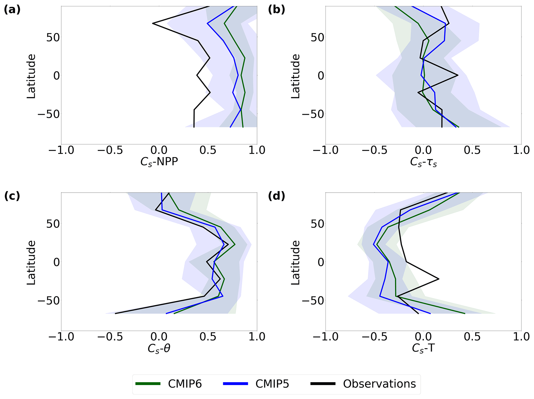
Figure 9The latitudinal profiles of the Pearson correlation coefficients between soil carbon and (a) NPP (Cs–NPP), (b) soil carbon turnover time (Cs–τs), (c) soil moisture (Cs–θ), and (d) temperature (Cs–T).
The spatial correlation between modelled soil carbon and soil moisture (Cs–θ) is consistent with the correlations seen in the benchmark datasets at every latitude, with an improvement seen in the tropical correlation patterns in CMIP6 compared with CMIP5 (Fig. 9c). Both the CMIP5 and CMIP6 ensembles span the benchmark Cs–θ correlation, though large model ranges in the Cs–θ sensitivity are seen across all latitudes. However, there is a reduced ensemble spread in the Cs–θ correlation from CMIP5 to CMIP6 at low- and mid-latitudes. An overestimation of the negative Cs–T correlation seen in the benchmark datasets is present in both the CMIP5 and CMIP6 models, except the high latitudes (Fig. 9d). This modelled Cs–T correlation is particularly underestimated at the lower tropical latitudes, where a greater positive correlation is seen here in the benchmark datasets. Figure 9d suggests a slight improvement in the modelled tropical Cs–T correlation in CMIP6 and a worsening of modelled Cs–T at the high latitudes than in CMIP5 when compared with the Cs–T correlations in the benchmark datasets.
4.1 Soil carbon stocks
4.1.1 Global total soil carbon
Simulating global soil carbon stocks that are consistent with empirical data is required to produce reliable projections of future soil carbon storage and emission (Todd-Brown et al., 2013). This study deduces a CMIP6 ensemble mean global total soil carbon of 1206 ± 445 PgC (Table 4), using regridded model resolutions (see Methods). It is noted that Ito (2011) states a CMIP6 ensemble of 1553 ± 672 PgC; however, the full soil carbon profile is considered for CESM2 and NorESM2-LM, as opposed to a depth of 1 m considered in this study. Additionally, this study deduces a comparable CMIP5 ensemble mean global soil carbon value of 1480 ± 810 PgC (Table 5) using equivalent dates in the historical simulation (1950–2000). Todd-Brown et al. (2013) state an ensemble mean soil carbon value of 1520 ± 770 PgC in CMIP5; however, the Todd-Brown et al. (2013) study includes the models BCC-CSM1.1, CESM1-CAM5, and INM-CM4, which are missing from the analysis in this study due to data availability. Anav et al. (2013) present a CMIP5 ensemble mean soil carbon value of 1502 ± 798 PgC, but this calculation includes multiple model versions (for example, LR and MR) from the same modelling centre in their ensemble. A caveat of this evaluation study is the non-independent nature of CMIP ESMs, where for example CESM2 and NorESM2-LM share the same LSM. Additionally, the ensembles included here do not necessarily represent all models that exist within each CMIP generation. However, the evaluation completed here allows for general improvements in the simulation of soil carbon stocks and fluxes between the CMIP5 and CMIP6 generations to be noted and key areas for future model development to be highlighted.
Despite a suggestion of a reduced spread in model estimates of global total soil carbon within CMIP6 relative to CMIP5, discrepancies remain in the consistency of these estimates with the observations between the two CMIP generations. It should also be noted that CMIP6 does not simply contain updated versions of every model in CMIP5: some new models are included and some CMIP5 models not included in CMIP6. These factors together with the uncertainty associated with empirical datasets have resulted in no robust conclusion being drawn on the improvement of soil carbon simulation in CMIP6 compared with CMIP5. Due to the potential significant feedback that exists between soil carbon and global climate, this lack of consistency reduces our confidence in future projections of climate change (Friedlingstein et al., 2006; Gregory et al., 2009; Arora et al., 2013; Friedlingstein et al., 2014).
4.1.2 Spatial soil carbon patterns
Modelled soil carbon was found to be poorly spatially correlated with the empirical data amongst models in both CMIP5 and CMIP6 (Fig. 4a). An improvement in CMIP6 ESMs was seen in the spatial patterns across the mid-latitudes, which were generally overestimated in CMIP5. However, significant underestimations of modelled soil carbon in the northern latitudes still remain, which have a significant impact on model predictions of global total soil carbon stocks (Fig. 1a). This systematic underestimation was previously reported in the literature as a limitation of the CMIP5 models, where Todd-Brown et al. (2013) found northern latitude soil carbon to be less consistent with the empirical data than on a global scale. This limitation remains amongst models in the CMIP6 generation, where it was found that the majority of CMIP6 models underestimate northern latitude soil carbon stocks regardless of whether the global soil carbon stocks are underestimated.
However, an exception to this northern latitude underestimation is seen within CMIP6 in the models CESM2 and NorESM2-LM. These ESMs include the land surface model (LSM) CLM5 (Lawrence et al., 2019), which is the first LSM to include the representation of vertically resolved soil carbon in its CMIP simulations. This representation enables the inclusion of separate carbon pools at varying depths in the soil, which aims to more consistently simulate soil carbon with the real world (Koven et al., 2013). This is of particular importance in the northern latitudes, where carbon stocks are expected to exist at much greater depths than the 1 m considered in this study (Tarnocai et al., 2009; Ran et al., 2022). This can be seen in Table 3, where increased magnitudes of soil carbon stocks are shown when increased depths are considered using the empirical datasets. A more thorough evaluation of soil carbon in both CESM2 and NorESM2-LM is suggested for future research, with a particular focus on this improved northern latitude soil carbon stock simulation; however, this evaluation of deeper soil carbon stocks (below 1 m) is beyond the scope of this study.
Accurately simulating soil carbon in the northern latitude regions is of particular importance as it is a major part of the total global soil carbon pool (Jackson et al., 2017). Additionally, much of the carbon stored in these soils is held within permafrost, which is known to be particularly sensitive to climate change. Permafrost thaw under climate change has the potential to release significant amounts of carbon into the atmosphere over a short period of time with increased warming (Schuur et al., 2015; Zimov et al., 2006; Burke et al., 2017; Hugelius et al., 2020), representing a positive feedback within the climate system. Permafrost dynamics are generally poorly represented in ESMs, where Burke et al. (2020) found CMIP6 ESMs to have a similar representation compared with CMIP5. Underestimating soil carbon in the northern latitudes may result in underestimation of the impact of this feedback in future climate change projections. Future improvements are needed to improve the simulation of soil carbon stocks globally, but particularly in the northern latitudes.
4.2 Drivers of soil carbon change
To allow for a more in-depth understanding of the inconsistencies found between modelled and empirical soil carbon, the simulation of above- and below-ground controls of soil carbon was also evaluated. Simulations of contemporary soil carbon can be disaggregated into the effects of litterfall, which is well approximated by plant NPP, and effective soil carbon turnover time (τs), which is affected by both the temperature and moisture of the soil (Koven et al., 2015). If models are to reliably simulate soil carbon in a way that is consistent with empirical data, the spatial drivers of soil carbon, NPP and τs, must also be simulated consistently with empirical data. Isolating the effects of NPP and τs on soil carbon helps us to break down the simulation of soil carbon to help understand the limitations and inconsistencies seen amongst the models.
4.2.1 NPP
An improved simulation of NPP is suggested in the ESMs included from CMIP6 compared with the ESMs from CMIP5. This conclusion is suggested by an increased number of models in our CMIP6 ensemble having global total NPP values consistent with empirical data (Table 6), the overestimation of tropical NPP amongst CMIP5 models being seen to be reduced amongst the CMIP6 models (Fig. 1b), and more agreement being seen within CMIP6 relative to CMIP5 in the simulation of mid-latitude and northern latitude NPP (Fig. 3b). Modelled NPP was found to be robustly more consistent with the empirical data in our CMIP6 ensemble compared with the CMIP5 ensemble in all statistical evaluation metrics. Since CMIP5, multiple models have seen an addition of a dynamic nitrogen cycle (Davies-Barnard et al., 2020), where the models with nitrogen cycles are highlighted in Fig. 5 by the shaded bars. The results suggest an improvement in the simulation of NPP with the addition of dynamic nitrogen in models. However, CMIP6 models that do not represent a nitrogen cycle also mostly see improvements in the simulation of NPP, suggesting NPP is more constrained by observations in the newest generation of models. CanESM5 is the only ESM within CMIP6 included here to not see an overall improvement in the simulation of NPP, where NPP is found to be overestimated compared with the benchmark dataset. It is likely that the inclusion of a nitrogen cycle in this model would limit this overestimated NPP and improve consistency with the observations (Zhang et al., 2014; Exbrayat et al., 2013).
Despite this apparent improved simulation of NPP in CMIP6, the spatial correlation between modelled soil carbon and NPP was found to be inconsistent with the equivalent empirically derived relationship. This result was previously shown for the CMIP5 models (Todd-Brown et al., 2013) and has been more recently shown for the CMIP6 models (Georgiou et al., 2021), both agreeing with the results found here. The majority of CMIP6 models were found to have positive Cs–NPP spatial correlations, as opposed to a negligible spatial correlation found in the observations (Fig. 8a). Despite NPP driving the spatial pattern of soil carbon stocks due to carbon input from vegetation, a positive correlation was not expected in the real world due to regions with high soil carbon not correlating with regions of high NPP. For example, in the observationally derived data, soil carbon stocks are greatest in the northern latitudes due to long turnover times in these regions, whereas NPP is lower due to cold temperatures in these regions limiting vegetation growth. The three CMIP6 models which did not significantly overestimate this correlation (CESM2, NorESM2-LM, and BCC-CSM2-MR) are three of the models with the most empirically consistent proportion of soil carbon stocks in the northern latitudes. Conversely, the tropical regions see high NPP values, but warmer temperatures result in faster turnover times and lower soil carbon stocks. NPP is expected to increase in the future under climate change (Kimball et al., 1993; Friedlingstein et al., 1995; Amthor, 1995), which means an overly positive correlation in models could result in a subsequent increase in modelled projections of soil carbon stocks. An overestimation of future soil carbon storage could result in an overestimation of the future carbon sink and an inaccurate global carbon budget (Todd-Brown et al., 2013; Friedlingstein et al., 2022).
4.2.2 Soil carbon turnover time
The systematic improvements suggested from the evaluation of NPP simulation within our CMIP6 ensemble are not suggested for the simulation of τs, where the simulation of τs appears to remain inconsistent with the empirical data in CMIP6 from CMIP5. Improvements are suggested within CMIP6 relative to CMIP5, such as more agreement within the ensemble at the mid-latitudes and in the tropical regions; however, less agreement is seen in the northern latitudes (Fig. 3c). Northern latitude τs is generally underestimated in models, which corresponds to the underestimation of soil carbon seen in these regions. This has been previously identified in ESMs, where it was found that the underestimation of global τs amongst the CMIP5 models is primarily due to low values in the northern latitudes (Wu et al., 2018). The reduced agreement in CMIP6 is due to long τs values existing in the northern latitudes of CESM2 and NorESM2-LM alongside the general ensemble underestimations (Fig. 7). The increased northern latitude τs values in CESM2 and NorESM2-LM are likely to be due to the representation of vertically resolved soil carbon pools, which allows for differential τs values for pools at varying depths. Despite these individual improvements since CMIP5, large discrepancies exist within the CMIP6 ensemble between modelled and empirical τs.
To simulate τs consistently with observations, the relationship of τs with both temperature (T) and moisture (θ) must also be simulated in a way that is consistent with observations. Generally, the τs–T relationship is consistently simulated; however, there is variation in the modelled temperature sensitivity of τs across the ensemble. The τs–θ relationship is less consistently represented, where the majority of CMIP6 models do not match the empirically derived relationship. Despite a positive dependence of soil respiration on soil moisture in the empirical data, many of the CMIP6 models display a contradictory positive τs–θ correlation (Fig. 8). Many of the models use functions that increase respiration with soil moisture (see Sect. 2.1), so the increase in τs with increasing soil moisture indicated by positive τs–θ correlations in the models is unexpected. We note that this effect occurs most strongly in the models with a very strongly negative τs–T relationship (Fig. 8c), so it could in fact be an artefact of a negative correlation between temperature and soil moisture. In this context it is also important to consider what soil moisture in LSMs represents (Koster et al., 2009). The aim within the models is to act as the lower boundary condition for atmospheric models, and therefore their soil parameters may historically have been tuned to give appropriate evaporation rates and not necessarily to represent the soil moisture itself in an accurate way, so it may be more relevant to consider the large-scale emergent patterns of τs than the direct relationships between soil moisture and respiration. It is noted that the empirical relationship shows τs reducing with higher soil moisture, which suggests that the observations are picking up more on longer turnover times in dry areas rather than in saturated areas such as peatlands. This may be due to having only surface soil moisture information, whereas peatlands, while saturated at depth, typically have a water table ∼ 10 cm below the surface and can be very dry at the surface (Evans et al., 2021). Thus, while models do not include the necessary processes for peat formation (Chadburn et al., 2022), this is unlikely to be the cause of the discrepancy since it would lead to even more of a positive τs–θ correlation in the models.
Different processes control soil carbon formation in different ecosystems, including stabilization by clay particles, transformation by microbes, and nitrogen and phosphorous availability (Witzgall et al., 2021). In the present study, the largest discrepancies in both soil carbon and turnover times are seen in permafrost and peatland areas (see Figs. 2 and 7). For example, the western Siberian peatland complex stands out in the majority of the panels in these figures as an area of high model error. This is partly because the soil carbon turnover times and quantities of soil carbon are largest in these regions but also partly because of the specific controlling processes in these ecosystems. A key part of soil carbon development in permafrost regions is the fact that organic material can be preserved in frozen soil, including via cryoturbation and yedoma deposits, which have not yet been thoroughly represented in models (Beer, 2016; Zhu et al., 2016). There are a variety of other factors, such as plants storing significantly more of their carbon below ground instead of above ground in cold climates and recalcitrant vegetation such as mosses, which are not represented in most ESMs (Sulman et al., 2021). Peatland formation is controlled primarily by waterlogging, which reduces the oxygen available for decomposition, but there are a huge number of additional physical and biogeochemical feedbacks that take place (Waddington et al., 2015). These kinds of small-scale processes and inhomogeneities are difficult to resolve in global models with ∼ 100 km2 grid cells, and this should be weighed up against their relative impact on global carbon budgets when considering including these processes in ESMs. However, it is suggested that the large-scale discrepancies such as in the permafrost and large peatland areas can and should be resolved in future model versions.
Our results suggest that much of the uncertainty associated with modelled soil carbon stocks can be attributed to the simulation of below-ground processes. The apparent improved consistency of NPP with empirical data suggests that considerable efforts have been made to achieve an improved representation of above-ground processes in CMIP6 ESMs since the release of the CMIP5 ensemble. However, the same improvements are not apparent in the simulation of τs as systemic limitations remain in the new generation of ESMs considered in this study, suggesting that the same progress in the model development of below-ground processes has not been achieved between CMIP5 and CMIP6. Moreover, focus on above-ground processes without consideration of below-ground processes can result in inconsistencies of soil carbon stocks. For example, the inclusion of a nitrogen cycle has been shown to lead to a reduction in soil carbon in the model (see Fig. 6 in Wiltshire et al., 2021), so tuning of the baseline turnover rates is required to keep soil carbon stocks consistent with observed values.
The required improvement of soil carbon pool turnover rates has previously been identified for the CMIP5 ensemble (Nishina et al., 2014), and more recently, Ito et al. (2020) found that the difference in turnover times amongst the CMIP6 models is responsible for approximately 88 % of the variation seen in global soil carbon stocks amongst the models and stated that constraining key parameters which control soil carbon turnover processes is a key area for future model development. A key development seen in CMIP6 since CMIP5 is the representation of vertically resolved soil carbon. Models which simulate non-vertically resolved soil carbon typically turn over all the carbon based on the temperature near the soil surface. This could lead to reduced quantities of soil carbon and an underestimation of northern latitude soil carbon stocks, due to near-surface soil being warmer than the deeper soil and as turnover is known to respond exponentially to temperature (Davidson and Janssens, 2006). Overall, further improvements in the representation of soil carbon turnover time, with a particular focus on the northern latitudes, are identified as a key area for future model development.
The ability of Earth system models (ESMs) to simulate present-day soil carbon is vital to help predict reliable global carbon budget estimates, which are required for Paris Agreement targets. In this study, CMIP6 ESMs have been evaluated against empirical datasets to assess their ability to represent soil carbon and related controls: net primary productivity (NPP) and the effective soil carbon turnover time (τs=Cs / Rh). The evaluation is completed by comparison with the previous generation of CMIP5 ESMs to assess where improvements have been made and to identify priorities for future model development. Below the key conclusions from this study are listed.
-
The spatial patterns of soil carbon in CMIP6 models appear to be more in agreement with each other than they were in CMIP5 and are more consistent with observations in the mid-latitudes, although caveats around the uncertainty in observations and the ensemble design make this conclusion uncertain. However, soil carbon is still heavily underestimated in high northern latitudes (with the exception of the two CMIP6 models that represent deep soil carbon).
-
Overall, we are not able to identify significant improvements in the simulation of the observed spatial pattern of soil carbon across the globe from the CMIP5 to CMIP6 generation.
-
There is good evidence that spatial patterns of contemporary NPP are better simulated in CMIP6 than in CMIP5 generation models when compared with satellite-derived estimates.
-
However, spatial patterns of τs continue to be poorly represented in CMIP6 models, in comparison with estimates derived from observational datasets of soil carbon and heterotrophic respiration (Rh).
-
Importantly, soil carbon simulations in both the CMIP5 and CMIP6 ESM generations seem to be spuriously highly correlated with NPP, which may make soil carbon in these models over-responsive to future projected changes in NPP.
Taken together, these conclusions point to a need for a much greater emphasis on improving the representation of below-ground soil processes in the next generation (CMIP7) of ESMs.

Figure A1Maps comparing empirical datasets of soil carbon (Cs). The benchmark dataset is a map plot showing Cs approximated to a depth of 1 m by combining the Harmonized World Soils Database (HWSD) (FAO and ISRIC, 2012) and Northern Circumpolar Soil Carbon Database (NCSCD) (Hugelius et al., 2013), where the NCSCD was used where overlap occurs. Additional map plots are shown for empirical Cs estimated by the World Inventory of Soil property Estimates (WISE30sec) (Batjes, 2016), the named “S2017” from Sanderman et al. (2017), the Global Soil Dataset for use in Earth system models (GSDE) (Shangguan et al., 2014), and the Global Gridded Surfaces of Selected Soil Characteristics (IGBP-DIS) (IGBP, 2000).
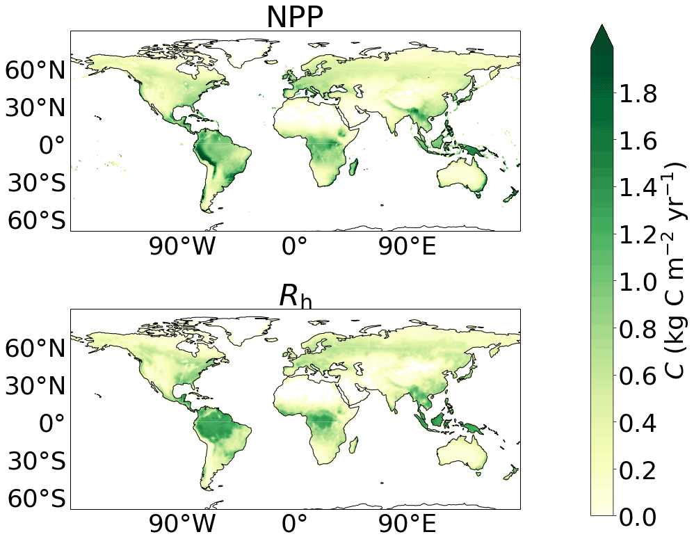
Figure A2Maps of empirical carbon flux datasets. Net primary production (NPP) is approximated using the MODIS NPP dataset (Zhao et al., 2005), and heterotrophic respiration (Rh) is approximated using the CARDAMOM Rh dataset (Bloom et al., 2015).
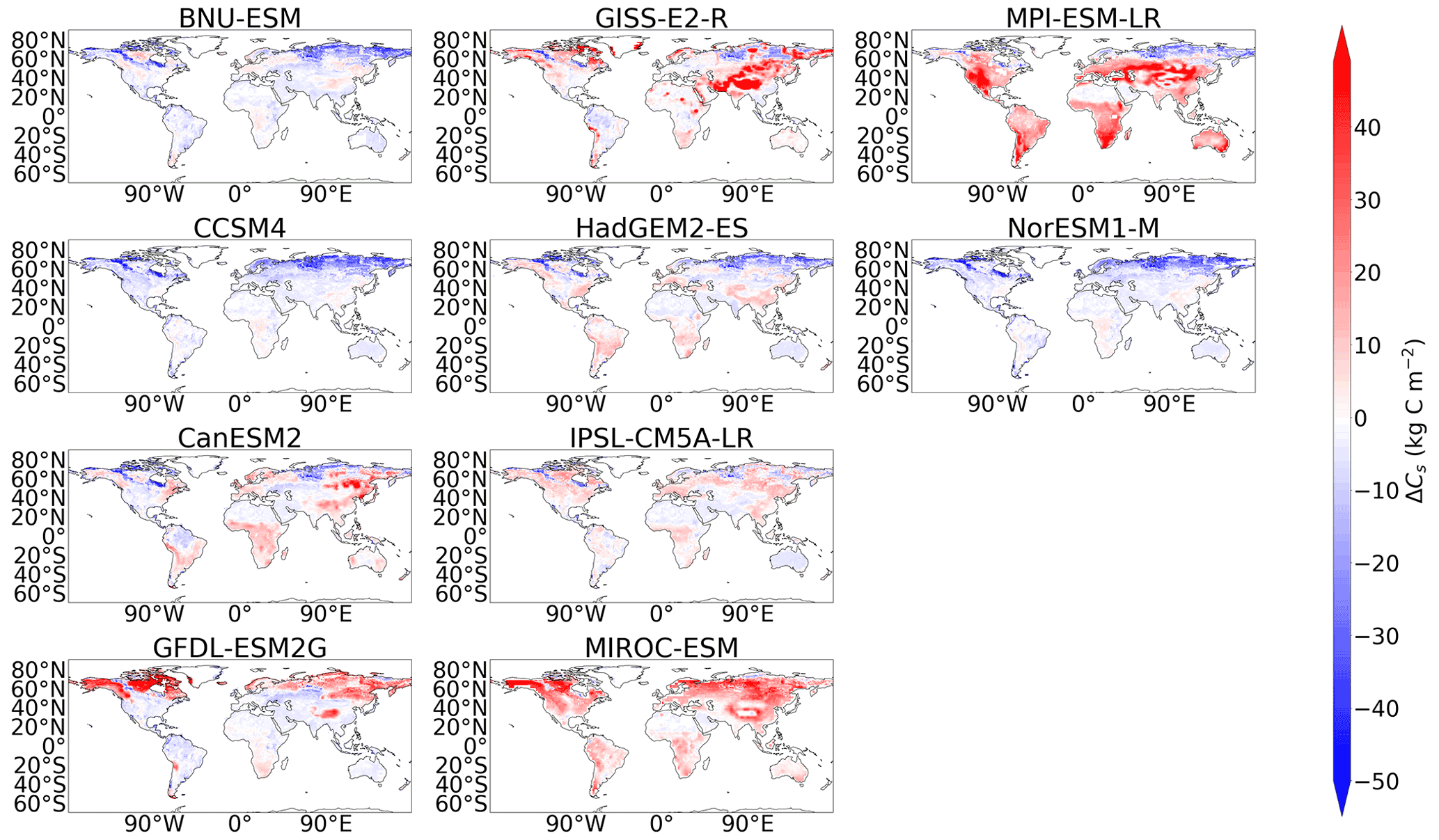
Figure A3Maps of the difference in soil carbon (Cs) between the historical simulation (1950–2000) for the CMIP5 models and the benchmark dataset.

Figure A4Maps of the difference in NPP between the historical simulation (1995–2005) for the CMIP5 models and the benchmark dataset.
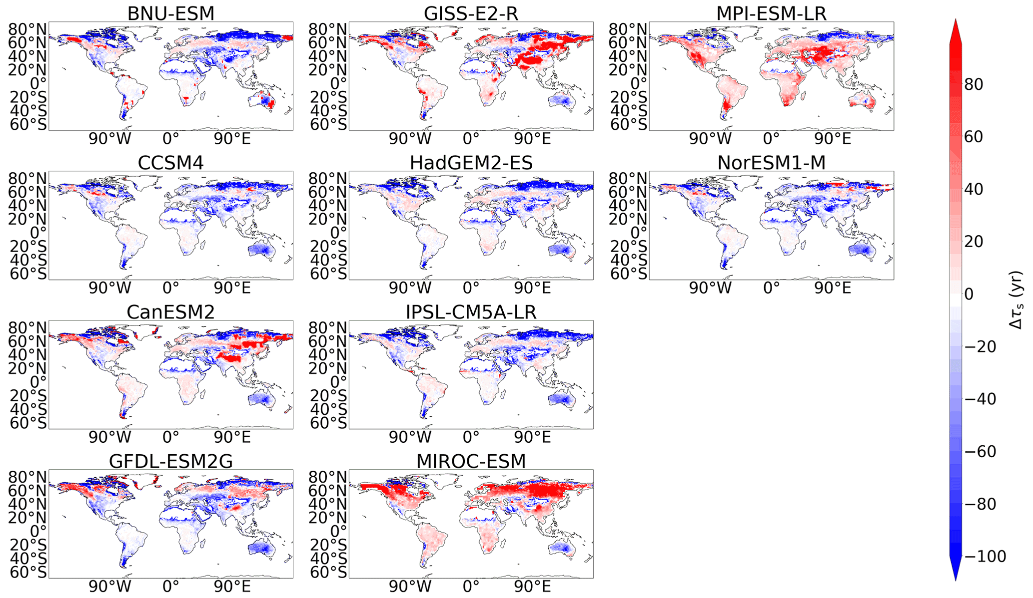
Figure A5Maps of the difference in τs between the historical simulation for the CMIP5 models and the benchmark datasets, where τs is defined as the ratio of Cs (1950–2000) to Rh (1995–2005).

Figure A6Maps of soil carbon (Cs) in the historical simulation (1950–2000) for the CMIP6 models.
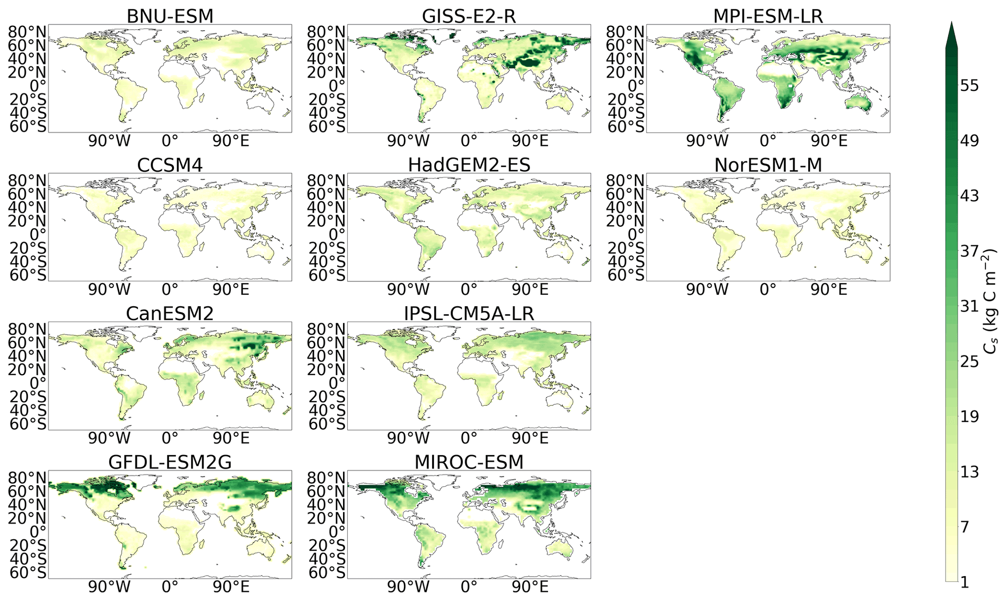
Figure A7Maps of soil carbon (Cs) in the historical simulation (1950–2000) for the CMIP5 models.
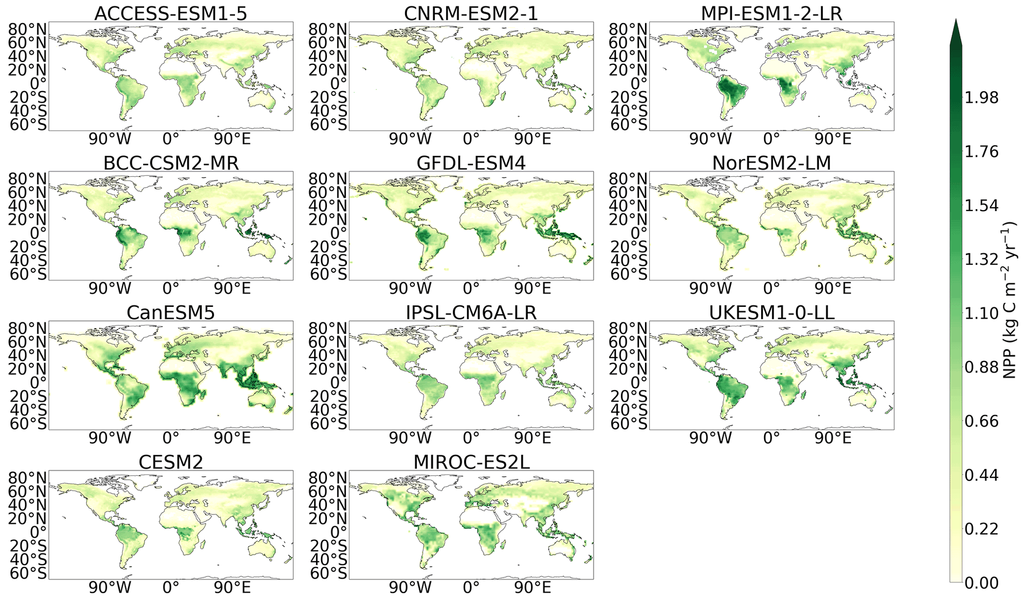
Figure A8Maps of NPP in the historical simulation (1995–2005) for the CMIP6 models.
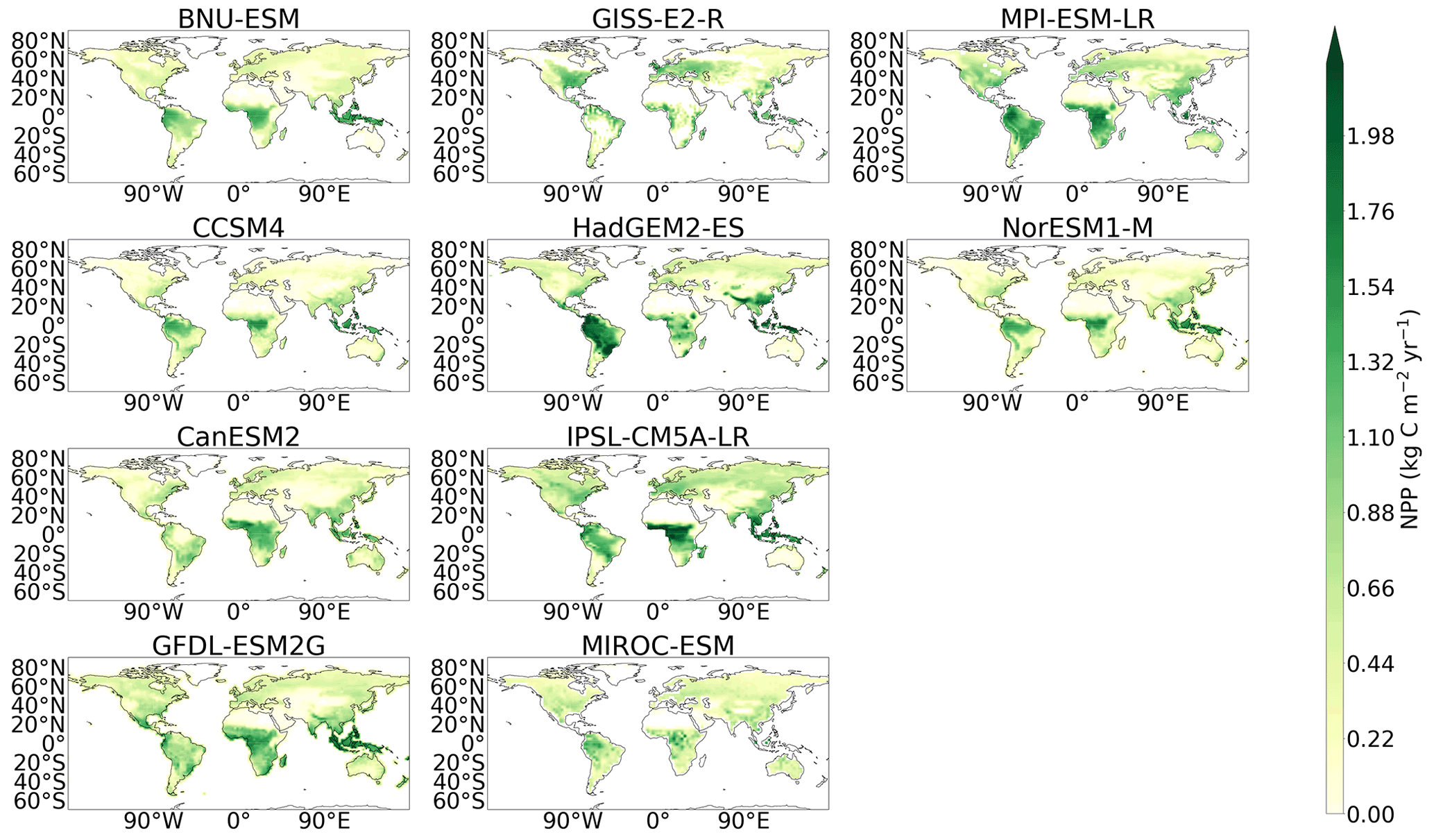
Figure A9Maps of NPP in the historical simulation (1995–2005) for the CMIP5 models.
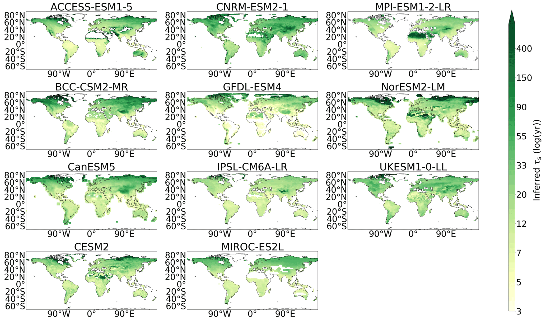
Figure A10Maps of soil carbon turnover times (τs) in the historical simulation for the CMIP6 models, where τs is defined as the ratio of Cs (1950–2000) to Rh (1995–2005).
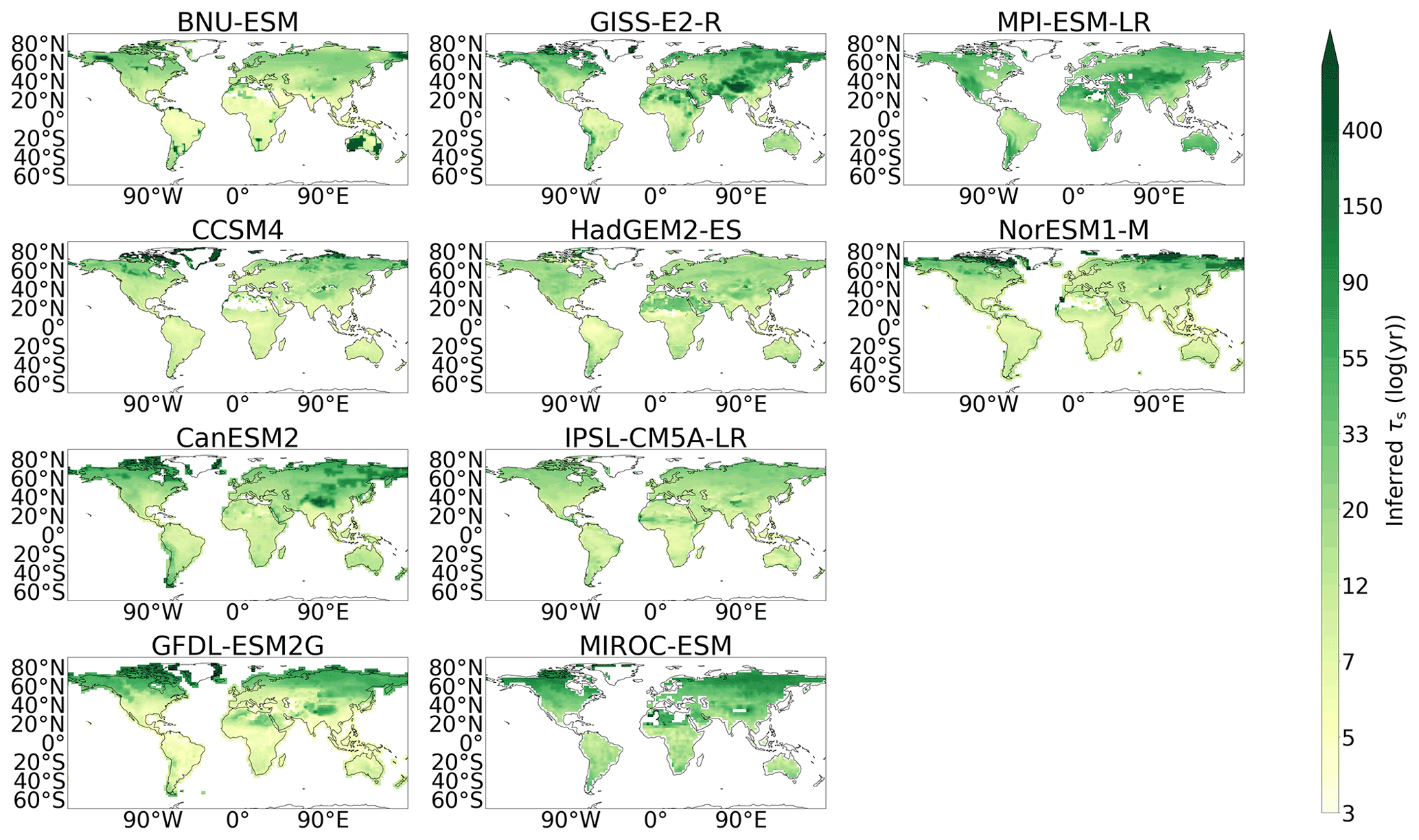
Figure A11Maps of soil carbon turnover times (τs) in the historical simulation for the CMIP5 models, where τs is defined as the ratio of Cs (1950–2000) to Rh (1995–2005).
Table A1Table presenting global carbon fluxes (PgC yr−1), NPP, and Rh for the 11 CMIP6 models included in this study and the empirical benchmark datasets.
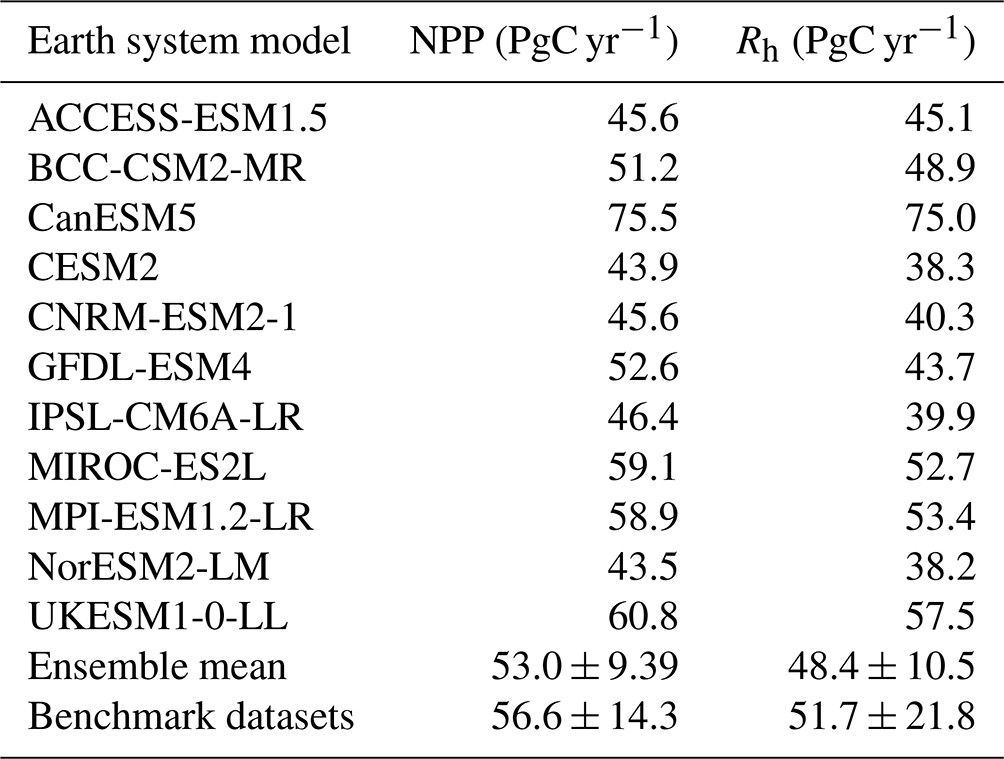
Table A2Table presenting global carbon fluxes (PgC yr−1), NPP, and Rh for the 10 CMIP5 models included in this study and the empirical benchmark datasets.
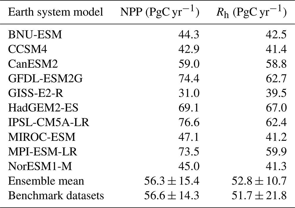
The datasets analysed during this study are available online: CMIP5 model output (https://esgf-node.llnl.gov/search/cmip5/, ESGF, 2022a), CMIP6 model output (https://esgf-node.llnl.gov/search/cmip6/, ESGF, 2022b), the Harmonized World Soils Database (HWSD) and Northern Circumpolar Soil Carbon Database (NCSCD) (https://github.com/rebeccamayvarney/CMIP_soilcarbon_evaluation, FAO and ISRIC, 2012; Hugelius et al., 2013), the World Inventory of Soil property Estimates (WISE30sec) (https://www.isric.org/explore/wise-databases, ISRIC World Soil Information Service, 2022), Sanderman et al. (2017) soil carbon estimates (1 and 2 m) (https://doi.org/10.7910/DVN/QQQM8V, HARVARD, 2022), the Global Soil Dataset for use in Earth system models (GSDE) (http://globalchange.bnu.edu.cn/research/soilw, Land-Atmosphere Interaction Research Group at Sun Yat-sen University, 2022), Global Gridded Surfaces of Selected Soil Characteristics (IGBP-DIS) (https://daac.ornl.gov/cgi-bin/dsviewer.pl?ds_id=569, ORNL-DAAC, 2022), MODIS net primary production (https://modis.gsfc.nasa.gov/data/dataprod/mod17.php, NASA, 2022), CARDAMOM heterotrophic respiration (https://datashare.ed.ac.uk/handle/10283/875, CARDAMOM, 2022), the Copernicus Climate Change Service (C3S) soil moisture gridded dataset (https://doi.org/10.24381/cds.d7782f18, Copernicus, 2022), and the WFDEI meteorological forcing data (https://rda.ucar.edu/datasets/ds314.2/, NCAR, 2022).
The supplement related to this article is available online at: https://doi.org/10.5194/bg-19-4671-2022-supplement.
RMV, SEC, and PMC outlined the evaluation and drafted the manuscript, and RMV completed the analysis and produced the figures. EJB provided the empirical datasets and gave helpful advice for addressing the empirical uncertainty. All the co-authors provided guidance on the study at various times and suggested edits to the draft manuscript.
The contact author has declared that none of the authors has any competing interests.
Publisher’s note: Copernicus Publications remains neutral with regard to jurisdictional claims in published maps and institutional affiliations.
We thank the World Climate Research Programme’s Working Group on Coupled Modelling, which is responsible for CMIP, and we thank the climate modelling groups for producing and making their model output available to enable studies such as this evaluation study. We also thank the providers of the empirical datasets, which enabled us to complete the evaluation in this study. The Taylor diagrams presented in this study were produced using the code available at https://gist.github.com/ycopin/3342888 (last access: 14 January 2022).
This research has been supported by the European Research Council, Emergent Constraints on Climate–Land feedbacks in the Earth System project (ECCLES; grant no. 742472), and the European Research Council, Climate–Carbon Interactions in the Current Century (4C) project (grant no. 821003) (Rebecca M. Varney and Peter M. Cox). Sarah E. Chadburn was supported by a Natural Environment Research Council independent research fellowship (grant no. NE/R015791/1). Eleanor J. Burke was supported by the Joint UK BEIS/Defra Met Office Hadley Centre Climate Programme (grant no. GA01101).
This paper was edited by Alexey V. Eliseev and reviewed by two anonymous referees.
Amthor, J. S.: Terrestrial higher-plant response to increasing atmospheric [CO2] in relation to the global carbon cycle, Global Change Biol., 1, 243–274, 1995. a
Anav, A., Friedlingstein, P., Kidston, M., Bopp, L., Ciais, P., Cox, P., Jones, C., Jung, M., Myneni, R., and Zhu, Z.: Evaluating the land and ocean components of the global carbon cycle in the CMIP5 Earth System Models, J. Climate, 26, 6801–6843, 2013. a, b, c, d
Arora, V. and Boer, G.: Uncertainties in the 20th century carbon budget associated with land use change, Global Change Biol., 16, 3327–3348, 2010. a
Arora, V., Boer, G., Christian, J., Curry, C., Denman, K., Zahariev, K., Flato, G., Scinocca, J., Merryfield, W., and Lee, W.: The effect of terrestrial photosynthesis down regulation on the twentieth-century carbon budget simulated with the CCCma Earth System Model, J. Climate, 22, 6066–6088, 2009. a
Arora, V. K., Boer, G. J., Friedlingstein, P., Eby, M., Jones, C. D., Christian, J. R., Bonan, G., Bopp, L., Brovkin, V., Cadule, P., Hajima, T., Ilyina, T., Lindsay, K., Tjiputra, J. F., and Wu, T.: Carbon–concentration and carbon–climate feedbacks in CMIP5 Earth system models, J. Climate, 26, 5289–5314, 2013. a, b, c
Arora, V. K., Katavouta, A., Williams, R. G., Jones, C. D., Brovkin, V., Friedlingstein, P., Schwinger, J., Bopp, L., Boucher, O., Cadule, P., Chamberlain, M. A., Christian, J. R., Delire, C., Fisher, R. A., Hajima, T., Ilyina, T., Joetzjer, E., Kawamiya, M., Koven, C. D., Krasting, J. P., Law, R. M., Lawrence, D. M., Lenton, A., Lindsay, K., Pongratz, J., Raddatz, T., Séférian, R., Tachiiri, K., Tjiputra, J. F., Wiltshire, A., Wu, T., and Ziehn, T.: Carbon–concentration and carbon–climate feedbacks in CMIP6 models and their comparison to CMIP5 models, Biogeosciences, 17, 4173–-4222, https://doi.org/10.5194/bg-17-4173-2020, 2020. a, b, c, d, e, f
Batjes, N. H.: Harmonized soil property values for broad-scale modelling (WISE30sec) with estimates of global soil carbon stocks, Geoderma, 269, 61–68, 2016. a, b, c
Beer, C.: Permafrost sub-grid heterogeneity of soil properties key for 3-D soil processes and future climate projections, Front. Earth Sci., 4, 81, https://doi.org/10.3389/feart.2016.00081, 2016. a
Bentsen, M., Bethke, I., Debernard, J. B., Iversen, T., Kirkevåg, A., Seland, Ø., Drange, H., Roelandt, C., Seierstad, I. A., Hoose, C., and Kristjánsson, J. E.: The Norwegian Earth System Model, NorESM1-M – Part 1: Description and basic evaluation of the physical climate, Geosci. Model Dev., 6, 687–-720, https://doi.org/10.5194/gmd-6-687-2013, 2013. a
Best, M. J., Pryor, M., Clark, D. B., Rooney, G. G., Essery, R. L. H., Ménard, C. B., Edwards, J. M., Hendry, M. A., Porson, A., Gedney, N., Mercado, L. M., Sitch, S., Blyth, E., Boucher, O., Cox, P. M., Grimmond, C. S. B., and Harding, R. J.: The Joint UK Land Environment Simulator (JULES), model description – Part 1: Energy and water fluxes, Geosci. Model Dev., 4, 677–699, https://doi.org/10.5194/gmd-4-677-2011, 2011. a
Bloom, A. and Williams, M.: CARDAMOM 2001–2010 global carbon Model-Data Fusion (MDF) analysis, https://doi.org/10.7488/ds/316, 2015. a, b
Boucher, O., Servonnat, J., Albright, A. L., Aumont, O., et al.: Presentation and evaluation of the IPSL-CM6A-LR climate model, J. Adv. Model. Earth Sy., 12, e2019MS002010, https://doi.org/10.1029/2019MS002010, 2020. a
Burke, E. J., Ekici, A., Huang, Y., Chadburn, S. E., Huntingford, C., Ciais, P., Friedlingstein, P., Peng, S., and Krinner, G.: Quantifying uncertainties of permafrost carbon–climate feedbacks, Biogeosciences, 14, 3051–-3066, https://doi.org/10.5194/bg-14-3051-2017, 2017. a
Burke, E. J., Zhang, Y., and Krinner, G.: Evaluating permafrost physics in the Coupled Model Intercomparison Project 6 (CMIP6) models and their sensitivity to climate change, The Cryosphere, 14, 3155–-3174, https://doi.org/10.5194/tc-14-3155-2020, 2020. a, b
Canadell, J., Monteiro, P., Costa, M., Cotrim da Cunha, L., Cox, P., Eliseev, A., Henson, S., Ishii, M., Jaccard, S., Koven, C., Lohila, A., Patra, P., Piao, S., Rogelj, J., Syampungani, S., Zaehle, S., and Zickfeld, K.: Global Carbon and other Biogeochemical Cycles and Feedbacks, Cambridge University Press, Cambridge, United Kingdom and New York, NY, USA, https://www.ipcc.ch/report/ar6/wg1/downloads/report/IPCC_AR6_WGI_Chapter05.pdf (last access: 28 July 2022), 2021. a
CARDAMOM: 2001–2010 global carbon Model-Data Fusion (MDF) analysis, DataShare Edinburgh [data set], https://datashare.ed.ac.uk/handle/10283/875, last access: 14 January 2022.
Carvalhais, N., Forkel, M., Khomik, M., Bellarby, J., Jung, M., Migliavacca, M., Mu, M., Saatchi, S., Santoro, M., Thurner, M., Weber, U., Ahrens, B., Beer, C., Cescatti, A., Randerson, J. T., and Reichstein, M.: Global covariation of carbon turnover times with climate in terrestrial ecosystems, Nature, 514, 213, https://doi.org/10.1038/nature13731, 2014. a, b, c
Chadburn, S. E., Burke, E. J., Gallego-Sala, A. V., Smith, N. D., Bret-Harte, M. S., Charman, D. J., Drewer, J., Edgar, C. W., Euskirchen, E. S., Fortuniak, K., Gao, Y., Nakhavali, M., Pawlak, W., Schuur, E. A. G., and Westermann, S.: A new approach to simulate peat accumulation, degradation and stability in a global land surface scheme (JULES vn5.8_accumulate_soil) for northern and temperate peatlands, Geosci. Model Dev., 15, 1633–1657, https://doi.org/10.5194/gmd-15-1633-2022, 2022. a
Cheruy, F., Ducharne, A., Hourdin, F., Musat, I., Vignon, É., Gastineau, G., Bastrikov, V., Vuichard, N., Diallo, B., Dufresne, J.-L., Ghattas, J., Grandpeix, J.-Y., Idelkadi, A., Mellul, L., Maignan, F., Ménégoz, M., Ottlé, C., Peylin, P., Servonnat, J., Wang, F., and Zhao, Y.: Improved near-surface continental climate in IPSL-CM6A-LR by combined evolutions of atmospheric and land surface physics, J. Adv. Model. Earth Sy., 12, e2019MS002005, https://doi.org/10.1029/2019MS002005, 2020. a
Clark, D. B., Mercado, L. M., Sitch, S., Jones, C. D., Gedney, N., Best, M. J., Pryor, M., Rooney, G. G., Essery, R. L. H., Blyth, E., Boucher, O., Harding, R. J., Huntingford, C., and Cox, P. M.: The Joint UK Land Environment Simulator (JULES), model description – Part 2: Carbon fluxes and vegetation dynamics, Geosci. Model Dev., 4, 701–-722, https://doi.org/10.5194/gmd-4-701-2011, 2011. a
Copernicus Climate Change Service, E. K.: Copernicus Climate Change Service, Product User Guide and Specification, https://datastore.copernicus-climate.eu/documents/satellite-soil-moisture/C3S_312b_Lot4.D3.SM.5-v3.0_202101_Product_User_Guide_Specification_i1.0.pdf (last access: 14 January 2022), 2021. a
Copernicus: Soil moisture gridded data from 1978 to present, Copernicus [data set], https://doi.org/10.24381/cds.d7782f18, 2022. a
Cox, P. M., Betts, R. A., Jones, C. D., Spall, S. A., and Totterdell, I. J.: Acceleration of global warming due to carbon-cycle feedbacks in a coupled climate model, Nature, 408, 184, https://doi.org/10.1038/35041539, 2000. a
Crowther, T. W., Todd-Brown, K. E. O., Rowe, C. W., Wieder, W. R., Carey, J. C., Machmuller, M. B., Snoek, B. L., Fang, S., Zhou, G., Allison, S. D., Blair, J. M., Bridgham, S. D., Burton, A. J., Carrillo, Y., Reich, P. B., Clark, J. S., Classen, A. T., Dijkstra, F. A., Elberling, B., Emmett, B. A., Estiarte, M., Frey, S. D., Guo, J., Harte, J., Jiang, L., Johnson, B. R., Kröel-Dulay, G., Larsen, K. S., Laudon, H., Lavallee, J. M., Luo, Y., Lupascu, M., Ma, L. N., Marhan, S., Michelsen, A., Mohan, J., Niu, S., Pendall, E., Peñuelas, J., Pfeifer-Meister, L., Poll, C., Reinsch, S., Reynolds, L. L., Schmidt, I. K., Sistla, S., Sokol, N. W., Templer, P. H., Treseder, K. K., Welker, J. M., and Bradford, M. A.: Quantifying global soil carbon losses in response to warming, Nature, 540, 104, https://doi.org/10.1038/nature20150, 2016. a
Dai, Y., Zeng, X., Dickinson, R. E., Baker, I., Bonan, G. B., Bosilovich, M. G., Denning, A. S., Dirmeyer, P. A., Houser, P. R., Niu, G., Oleson, K. W., Schlosser, C. A., and Yang, Z.-L.: The common land model, B. Am. Meteorol. Soc., 84, 1013–1024, 2003. a
Danabasoglu, G., Lamarque, J.-F., Bacmeister, J., Bailey, D., DuVivier, A., Edwards, J., Emmons, L., Fasullo, J., Garcia, R., Gettelman, A., Hannay, C., Holland, M. M., Large, W. G., Lauritzen, P. H., Lawrence, D. M., Lenaerts, J. T. M., Lindsay, K., Lipscomb, W. H., Mills, M. J., Neale, R., Oleson, K. W., Otto-Bliesner, B., Phillips, A. S., Sacks, W., Tilmes, S., van Kampenhout, L., Vertenstein, M., Bertini, A., Dennis, J., Deser, C., Fischer, C., Fox-Kemper, B., Kay, J. E., Kinnison, D., Kushner, P. J., Larson, V. E., Long, M. C., Mickelson, S., Moore, J. K., Nienhouse, E., Polvani, L., Rasch, P. J., and Strand, W. G.: The community earth system model version 2 (CESM2), J. Adv. Model. Earth Sy., 12, e2019MS001916, https://doi.org/10.1029/2019MS001916, 2020. a
Davidson, E. A. and Janssens, I. A.: Temperature sensitivity of soil carbon decomposition and feedbacks to climate change, Nature, 440, 165, https://doi.org/10.1038/nature04514, 2006. a, b
Davies-Barnard, T., Meyerholt, J., Zaehle, S., Friedlingstein, P., Brovkin, V., Fan, Y., Fisher, R. A., Jones, C. D., Lee, H., Peano, D., Smith, B., Wårlind, D., and Wiltshire, A. J.: Nitrogen cycling in CMIP6 land surface models: progress and limitations, Biogeosciences, 17, 5129–-5148, https://doi.org/10.5194/bg-17-5129-2020, 2020. a
Del Grosso, S., Parton, W., Mosier, A., Holland, E., Pendall, E., Schimel, D., and Ojima, D.: Modeling soil CO2 emissions from ecosystems, Biogeochemistry, 73, 71–91, 2005. a
Delire, C., Séférian, R., Decharme, B., Alkama, R., Calvet, J.-C., Carrer, D., Gibelin, A.-L., Joetzjer, E., Morel, X., Rocher, M., and Diane Tzanos, D.: The global land carbon cycle simulated with ISBA-CTRIP: Improvements over the last decade, J. Adv. Model. Earth Sy., 12, e2019MS001886, https://doi.org/10.1029/2019MS001886, 2020. a
Dorigo, W., Wagner, W., Albergel, C., Albrecht, F., Balsamo, G., Brocca, L., Chung, D., Ertl, M., Forkel, M., Gruber, A., Haas, E., Hamer, P. D., Hirschi, M., Ikonen, J., de Jeu, R., Kidd, R., Lahoz, W., Liu, Y. Y., Miralles, D., Mistelbauer, T., Nicolai-Shaw, N., Parinussa, R., Pratola, C., Reimer, C., van der Schalie, R., Seneviratne, S. I., Smolander, T., and Lecomte, P.: ESA CCI Soil Moisture for improved Earth system understanding: State-of-the art and future directions, Remote Sens. Environ., 203, 185–215, 2017. a
Dufresne, J.-L., Foujols, M.-A., Denvil, S., Caubel, A., Marti, O., Aumont, O., Balkanski, Y., Bekki, S., Bellenger, H., Benshila, R., Bony, S., Bopp, L., Braconnot, P., Brockmann, P., Cadule, P., Cheruy, F., Codron, F., Cozic, A., Cugnet, D., de Noblet, N., Duvel, J.-P., Ethé, C., Fairhead, L., Fichefet, T., Flavoni, S., Friedlingstein, P., Grandpeix, J.-Y., Guez, L., Guilyardi, E., Hauglustaine, D., Hourdin, F., Idelkadi, A., Ghattas, J., Joussaume, S., Kageyama, M., Krinner, G., Labetoulle, S., Lahellec, A., Lefebvre, M.-P., Lefevre, F., Levy, C., Li, Z. X., Lloyd, J., Lott, F., Madec, G., Mancip, M., Marchand, M., Masson, S., Meurdesoif, Y., Mignot, J., Musat, I., Parouty, S., Polcher, J., Rio, C., Schulz, M., Swingedouw, D., Szopa, S., Talandier, C., Terray, P., Viovy, N., and Vuichard, N.: Climate change projections using the IPSL-CM5 Earth System Model: from CMIP3 to CMIP5, Clim. Dynam., 40, 2123–2165, 2013. a
Dunne, J. P., Horowitz, L. W., Adcroft, A. J., Ginoux, P., Held, I. M., John, J. G., Krasting, J. P., Malyshev, S., Naik, V., Paulot, F., Shevliakova, E., Stock, C. A., Zadeh, N., Balaji, V., Blanton, C., Dunne, K. A., Dupuis, C., Durachta, J., Dussin, R., Gauthier, P. P. G., Griffies, S. M., Guo, H., Hallberg, R. W., Harrison, M., He, J., Hurlin, W., McHugh, C., Menzel, R., Milly, P. C. D., Nikonov, S., Paynter, D. J., Ploshay, J., Radhakrishnan, A., Rand, K., Reichl, B. G., Robinson, T., Schwarzkopf, D. M., Sentman, L. T., Underwood, S., Vahlenkamp, H., Winton, M., Wittenberg, A. T., Wyman B., Zeng, Y., and Zhao, M.: The GFDL Earth System Model version 4.1 (GFDL-ESM 4.1): Overall coupled model description and simulation characteristics, J. Adv. Model. Earth Sy., 12, e2019MS002015, https://doi.org/10.1029/2019MS002015, 2020. a
Dunne, J. P., John, J. G., Adcroft, A. J., Griffies, S. M., Hallberg, R. W., Shevliakova, E., Stouffer, R. J., Cooke, W., Dunne, K. A., Harrison, M. J., Krasting, J. P., Malyshev, S. L., Milly, P. C. D., Phillipps, P. J., Sentman, L. T., Samuels, B. L., Spelman, M. J., Winton, M., Wittenberg, A. T., and Zadeh, N.: GFDL’s ESM2 global coupled climate–carbon earth system models. Part I: Physical formulation and baseline simulation characteristics, J. Climate, 25, 6646–6665, 2012. a
Dunne, J. P., John, J. G., Shevliakova, E., Stouffer, R. J., Krasting, J. P., Malyshev, S. L., Milly, P., Sentman, L. T., Adcroft, A. J., Cooke, W., Dunne, K. A., Griffies, S. M., Hallberg, R. W., Harrison, M. J., Levy, H., Wittenberg, A. T., Phillips, P. J., and Zadeh, N.: GFDL’s ESM2 global coupled climate–carbon earth system models. Part II: carbon system formulation and baseline simulation characteristics, J. Climate, 26, 2247–2267, 2013. a
ESGF: WCRP Coupled Model Intercomparison Project (Phase 5), CMIP5 [data set], https://esgf-node.llnl.gov/search/cmip5/ (last access: 12 April 2022), 2022a.
ESGF: WCRP Coupled Model Intercomparison Project (Phase 6), CMIP [data set], https://esgf-node.llnl.gov/search/cmip6/ (last access: 12 April 2022), 2022b.
Eswaran, H., Van Den Berg, E., and Reich, P.: Organic carbon in soils of the world, Soil Sci. Soc. Am. J., 57, 192–194, 1993. a
Evans, C., Peacock, M., Baird, A., et al.: Overriding water table control on managed peatland greenhouse gas emissions, Nature, 593, 548–552, 2021. a
Exbrayat, J.-F., Pitman, A. J., Zhang, Q., Abramowitz, G., and Wang, Y.-P.: Examining soil carbon uncertainty in a global model: response of microbial decomposition to temperature, moisture and nutrient limitation, Biogeosciences, 10, 7095–-7108, https://doi.org/10.5194/bg-10-7095-2013, 2013. a
Eyring, V., Bony, S., Meehl, G. A., Senior, C. A., Stevens, B., Stouffer, R. J., and Taylor, K. E.: Overview of the Coupled Model Intercomparison Project Phase 6 (CMIP6) experimental design and organization, Geosci. Model Dev., 9, 1937–-1958, https://doi.org/10.5194/gmd-9-1937-2016, 2016. a, b
FAO, I. and ISRIC, I.: JRC: Harmonized World Soil Database (version 1.2), FAO, Rome, Italy and IIASA, Laxenburg, Austria, https://doi.org/10.3334/ORNLDAAC/1247, 2012 (data available at: https://github.com/rebeccamayvarney/CMIP_soilcarbon_evaluation, last access: 14 January 2022). a, b, c, d
Friedlingstein, P., Fung, I., Holland, E., John, J., Brasseur, G., Erickson, D., and Schimel, D.: On the contribution of CO2 fertilization to the missing biospheric sink, Global Biogeochem. Cy., 9, 541–556, 1995. a
Friedlingstein, P., Cox, P., Betts, R., Bopp, L., von Bloh, W., Brovkin, V., Cadule, P., Doney, S., Eby, M., Fung, I., Bala, G., John, J., Jones, C., Joos, F., Kato, T., Kawamiya, M., Knorr, W., Lindsay, K., Matthews, H. D., Raddatz, T., Rayner, P., Reick, C., Roeckner, E., Schnitzler, K.-G., Schnur, R., Strassmann, K., Weaver, A. J., Yoshikawa, C., and Zeng, N.: Climate–carbon cycle feedback analysis: results from the C4MIP model intercomparison, J. Clim., 19, 3337–3353, 2006. a, b
Friedlingstein, P., Meinshausen, M., Arora, V. K., Jones, C. D., Anav, A., Liddicoat, S. K., and Knutti, R.: Uncertainties in CMIP5 climate projections due to carbon cycle feedbacks, J. Climate, 27, 511–526, 2014. a, b, c
Friedlingstein, P., Jones, M. W., O'Sullivan, M., Andrew, R. M., Bakker, D. C. E., Hauck, J., Le Quéré, C., Peters, G. P., Peters, W., Pongratz, J., Sitch, S., Canadell, J. G., Ciais, P., Jackson, R. B., Alin, S. R., Anthoni, P., Bates, N. R., Becker, M., Bellouin, N., Bopp, L., Chau, T. T. T., Chevallier, F., Chini, L. P., Cronin, M., Currie, K. I., Decharme, B., Djeutchouang, L. M., Dou, X., Evans, W., Feely, R. A., Feng, L., Gasser, T., Gilfillan, D., Gkritzalis, T., Grassi, G., Gregor, L., Gruber, N., Gürses, Ö., Harris, I., Houghton, R. A., Hurtt, G. C., Iida, Y., Ilyina, T., Luijkx, I. T., Jain, A., Jones, S. D., Kato, E., Kennedy, D., Klein Goldewijk, K., Knauer, J., Korsbakken, J. I., Körtzinger, A., Landschützer, P., Lauvset, S. K., Lefèvre, N., Lienert, S., Liu, J., Marland, G., McGuire, P. C., Melton, J. R., Munro, D. R., Nabel, J. E. M. S., Nakaoka, S.-I., Niwa, Y., Ono, T., Pierrot, D., Poulter, B., Rehder, G., Resplandy, L., Robertson, E., Rödenbeck, C., Rosan, T. M., Schwinger, J., Schwingshackl, C., Séférian, R., Sutton, A. J., Sweeney, C., Tanhua, T., Tans, P. P., Tian, H., Tilbrook, B., Tubiello, F., van der Werf, G. R., Vuichard, N., Wada, C., Wanninkhof, R., Watson, A. J., Willis, D., Wiltshire, A. J., Yuan, W., Yue, C., Yue, X., Zaehle, S., and Zeng, J.: Global Carbon Budget 2021, Earth Syst. Sci. Data, 14, 1917–-2005, https://doi.org/10.5194/essd-14-1917-2022, 2022. a, b
Gent, P. R., Danabasoglu, G., Donner, L. J., Holland, M. M., Hunke, E. C., Jayne, S. R., Lawrence, D. M., Neale, R. B., Rasch, P. J., Vertenstein, M., Worley, P. H., Yang, Z.-L., and Zhang, M.: The community climate system model version 4, J. Climate, 24, 4973–4991, 2011. a
Georgiou, K., Malhotra, A., Wieder, W. R., Ennis, J. H., Hartman, M. D., Sulman, B. N., Berhe, A. A., Grandy, A. S., Kyker-Snowman, E., Lajtha, K., Moore, J. A. M., Pierson, D., and Jackson, R. B.: Divergent controls of soil organic carbon between observations and process-based models, Biogeochemistry, 156, 5–17, 2021. a
Goll, D. S., Brovkin, V., Liski, J., Raddatz, T., Thum, T., and Todd-Brown, K. E.: Strong dependence of CO2 emissions from anthropogenic land cover change on initial land cover and soil carbon parametrization, Global Biogeochem. Cy., 29, 1511–1523, 2015. a
Goll, D. S., Winkler, A. J., Raddatz, T., Dong, N., Prentice, I. C., Ciais, P., and Brovkin, V.: Carbon–nitrogen interactions in idealized simulations with JSBACH (version 3.10), Geosci. Model Dev., 10, 2009–-2030, https://doi.org/10.5194/gmd-10-2009-2017, 2017. a
Gregory, J. M., Jones, C., Cadule, P., and Friedlingstein, P.: Quantifying carbon cycle feedbacks, J. Climate, 22, 5232–5250, 2009. a, b
Gruber, A., Dorigo, W. A., Crow, W., and Wagner, W.: Triple collocation-based merging of satellite soil moisture retrievals, IEEE T. Geosci. Remote, 55, 6780–6792, 2017. a
Guimberteau, M., Zhu, D., Maignan, F., Huang, Y., Yue, C., Dantec-Nédélec, S., Ottlé, C., Jornet-Puig, A., Bastos, A., Laurent, P., Goll, D., Bowring, S., Chang, J., Guenet, B., Tifafi, M., Peng, S., Krinner, G., Ducharne, A., Wang, F., Wang, T., Wang, X., Wang, Y., Yin, Z., Lauerwald, R., Joetzjer, E., Qiu, C., Kim, H., and Ciais, P.: ORCHIDEE-MICT (v8.4.1), a land surface model for the high latitudes: model description and validation, Geosci. Model Dev., 11, 121–-163, https://doi.org/10.5194/gmd-11-121-2018, 2018. a
Hajima, T., Watanabe, M., Yamamoto, A., Tatebe, H., Noguchi, M. A., Abe, M., Ohgaito, R., Ito, A., Yamazaki, D., Okajima, H., Ito, A., Takata, K., Ogochi, K., Watanabe, S., and Kawamiya, M.: Development of the MIROC-ES2L Earth system model and the evaluation of biogeochemical processes and feedbacks, Geosci. Model Dev., 13, 2197–-2244, https://doi.org/10.5194/gmd-13-2197-2020, 2020. a
Harper, A. B., Wiltshire, A. J., Cox, P. M., Friedlingstein, P., Jones, C. D., Mercado, L. M., Sitch, S., Williams, K., and Duran-Rojas, C.: Vegetation distribution and terrestrial carbon cycle in a carbon cycle configuration of JULES4.6 with new plant functional types, Geosci. Model Dev., 11, 2857–-2873, https://doi.org/10.5194/gmd-11-2857-2018, 2018. a
HARVARD dataverse: Soil carbon profile data from paired land use comparisons, Harvard Dataverse [data set], https://doi.org/10.7910/DVN/QQQM8V, 2022.
Haverd, V., Smith, B., Nieradzik, L., Briggs, P. R., Woodgate, W., Trudinger, C. M., Canadell, J. G., and Cuntz, M.: A new version of the CABLE land surface model (Subversion revision r4601) incorporating land use and land cover change, woody vegetation demography, and a novel optimisation-based approach to plant coordination of photosynthesis, Geosci. Model Dev., 11, 2995–-3026, https://doi.org/10.5194/gmd-11-2995-2018, 2018. a
Hugelius, G., Tarnocai, C., Broll, G., Canadell, J. G., Kuhry, P., and Swanson, D. K.: The Northern Circumpolar Soil Carbon Database: spatially distributed datasets of soil coverage and soil carbon storage in the northern permafrost regions, Earth Syst. Sci. Data, 5, 3–13, https://doi.org/10.5194/essd-5-3-2013, 2013 (data available at: https://github.com/rebeccamayvarney/CMIP_soilcarbon_evaluation, last access: 14 January 2022). a, b, c, d
Hugelius, G., Loisel, J., Chadburn, S., Jackson, R. B., Jones, M., MacDonald, G., Marushchak, M., Olefeldt, D., Packalen, M., Siewert, M. B., Treat, C., Turetsky, M., Voigt, C., and Yu, Z.: Large stocks of peatland carbon and nitrogen are vulnerable to permafrost thaw, P. Natl. Acad. Sci. USA, 117, 20438–20446, 2020. a
IGBP: Global Gridded Surfaces of Selected Soil Characteristics (IGBP-DIS), DAAC [data set], https://doi.org/10.3334/ORNLDAAC/569, 2000. a, b, c
IPCC, 2021: Climate Change 2021: The Physical Science Basis. Contribution of Working Group I to the Sixth Assessment Report of the Intergovernmental Panel on Climate Change, edited by: Masson-Delmotte, V., Zhai, P., Pirani, A., Connors, S. L., Péan, C., Berger, S., Caud, N., Chen, Y., Goldfarb, L., Gomis, M. I., Huang, M., Leitzell, K., Lonnoy, E., Matthews, J. B. R., Maycock, T. K., Waterfield, T., Yelekçi, O., Yu, R., and Zhou, B., Cambridge University Press, Cambridge, United Kingdom and New York, NY, USA, 2391 pp., 2021. a
ISRIC World Soil Information Service (WoSIS): WISE Soil Property Databases, ISRIC [data set], https://www.isric.org/explore/wise-databases, last access: 14 January 2022. a
Ito, A.: A historical meta-analysis of global terrestrial net primary productivity: are estimates converging?, Global Change Biol., 17, 3161–3175, 2011. a, b, c
Ito, A. and Oikawa, T.: A simulation model of the carbon cycle in land ecosystems (Sim-CYCLE): a description based on dry-matter production theory and plot-scale validation, Ecol. Model., 151, 143–176, 2002. a, b
Ito, A., Hajima, T., Lawrence, D. M., Brovkin, V., Delire, C., Guenet, B., Jones, C. D., Malyshev, S., Materia, S., McDermid, S. P., Peano, D., Pongratz, J., Robertson, E., Shevliakova, E., Vuichard, N., Wårlind, D., Wiltshire, A., and Ziehn, T.: Soil carbon sequestration simulated in CMIP6-LUMIP models: implications for climatic mitigation, Environ. Res. Lett., 15, 124061, https://doi.org/10.1088/1748-9326/abc912, 2020. a, b, c
Iversen, T., Bentsen, M., Bethke, I., Debernard, J. B., Kirkevåg, A., Seland, Ø., Drange, H., Kristjansson, J. E., Medhaug, I., Sand, M., and Seierstad, I. A.: The Norwegian Earth System Model, NorESM1-M – Part 2: Climate response and scenario projections, Geosci. Model Dev., 6, 389–-415, https://doi.org/10.5194/gmd-6-389-2013, 2013. a
Jackson, R. B., Lajtha, K., Crow, S. E., Hugelius, G., Kramer, M. G., and Piñeiro, G.: The ecology of soil carbon: pools, vulnerabilities, and biotic and abiotic controls, Annu. Rev. Ecol. Evol. S., 48, 419–445, 2017. a, b
Ji, D., Wang, L., Feng, J., Wu, Q., Cheng, H., Zhang, Q., Yang, J., Dong, W., Dai, Y., Gong, D., Zhang, R.-H., Wang, X., Liu, J., Moore, J. C., Chen, D., and Zhou, M.: Description and basic evaluation of Beijing Normal University Earth System Model (BNU-ESM) version 1, Geosci. Model Dev., 7, 2039-–2064, https://doi.org/10.5194/gmd-7-2039-2014, 2014. a, b
Ji, J., Huang, M., and Li, K.: Prediction of carbon exchanges between China terrestrial ecosystem and atmosphere in 21st century, Sci. China Ser. D, 51, 885–898, 2008. a
Jobbágy, E. G. and Jackson, R. B.: The vertical distribution of soil organic carbon and its relation to climate and vegetation, Ecol. Appl., 10, 423–436, 2000. a
Jones, C. D., Hughes, J. K., Bellouin, N., Hardiman, S. C., Jones, G. S., Knight, J., Liddicoat, S., O'Connor, F. M., Andres, R. J., Bell, C., Boo, K.-O., Bozzo, A., Butchart, N., Cadule, P., Corbin, K. D., Doutriaux-Boucher, M., Friedlingstein, P., Gornall, J., Gray, L., Halloran, P. R., Hurtt, G., Ingram, W. J., Lamarque, J.-F., Law, R. M., Meinshausen, M., Osprey, S., Palin, E. J., Parsons Chini, L., Raddatz, T., Sanderson, M. G., Sellar, A. A., Schurer, A., Valdes, P., Wood, N., Woodward, S., Yoshioka, M., and Zerroukat, M.: The HadGEM2-ES implementation of CMIP5 centennial simulations, Geosci. Model Dev., 4, 543–-570, https://doi.org/10.5194/gmd-4-543-2011, 2011. a
Kimball, B., Mauney, J., Nakayama, F., and Idso, S.: Effects of increasing atmospheric CO2 on vegetation, Vegetatio, 104, 65–75, 1993. a
Knorr, W.: Annual and interannual CO2 exchanges of the terrestrial biosphere: Process-based simulations and uncertainties, Global Ecol. Biogeogr., 9, 225–252, 2000. a
Koster, R. D., Guo, Z., Yang, R., Dirmeyer, P. A., Mitchell, K., and Puma, M. J.: On the nature of soil moisture in land surface models, J. Climate, 22, 4322–4335, 2009. a
Koven, C. D., Riley, W. J., Subin, Z. M., Tang, J. Y., Torn, M. S., Collins, W. D., Bonan, G. B., Lawrence, D. M., and Swenson, S. C.: The effect of vertically resolved soil biogeochemistry and alternate soil C and N models on C dynamics of CLM4, Biogeosciences, 10, 7109–-7131, https://doi.org/10.5194/bg-10-7109-2013, 2013 a
Koven, C. D., Chambers, J. Q., Georgiou, K., Knox, R., Negron-Juarez, R., Riley, W. J., Arora, V. K., Brovkin, V., Friedlingstein, P., and Jones, C. D.: Controls on terrestrial carbon feedbacks by productivity versus turnover in the CMIP5 Earth System Models, Biogeosciences, 12, 5211–-5228, https://doi.org/10.5194/bg-12-5211-2015, 2015. a, b, c, d
Koven, C. D., Hugelius, G., Lawrence, D. M., and Wieder, W. R.: Higher climatological temperature sensitivity of soil carbon in cold than warm climates, Nat. Clim. Change, 7, 817, https://doi.org/10.1038/nclimate3421, 2017. a, b, c
Krinner, G., Viovy, N., de Noblet-Ducoudré, N., Ogée, J., Polcher, J., Friedlingstein, P., Ciais, P., Sitch, S., and Prentice, I. C.: A dynamic global vegetation model for studies of the coupled atmosphere-biosphere system, Global Biogeochem. Cy., 19, GB1015, https://doi.org/10.1029/2003GB002199, 2005. a
Land-Atmosphere Interaction Research Group at Sun Yat-sen University: Global Soil Dataset [data set], http://globalchange.bnu.edu.cn/research/soilw, last access: 14 January 2022.
Lawrence, D. M., Oleson, K. W., Flanner, M. G., Thornton, P. E., Swenson, S. C., Lawrence, P. J., Zeng, X., Yang, Z.-L., Levis, S., Sakaguchi, K., Bonan, G. B., and Slater, A. G.: Parameterization improvements and functional and structural advances in version 4 of the Community Land Model, J. Adv. Model. Earth Sy., 3, M03001, https://doi.org/10.1029/2011MS00045, 2011. a, b
Lawrence, D. M., Fisher, R. A., Koven, C. D., et al.: The Community Land Model version 5: Description of new features, benchmarking, and impact of forcing uncertainty, J. Adv. Model. Earth Sy., 11, 4245–4287, 2019. a, b, c, d, e
Liu, Y., Dorigo, W. A., Parinussa, R., de Jeu, R. A., Wagner, W., McCabe, M. F., Evans, J., and Van Dijk, A.: Trend-preserving blending of passive and active microwave soil moisture retrievals, Remote Sens. Environ., 123, 280–297, 2012. a
Liu, Y. Y., Parinussa, R. M., Dorigo, W. A., De Jeu, R. A. M., Wagner, W., van Dijk, A. I. J. M., McCabe, M. F., and Evans, J. P.: Developing an improved soil moisture dataset by blending passive and active microwave satellite-based retrievals, Hydrol. Earth Syst. Sci., 15, 425–-436, https://doi.org/10.5194/hess-15-425-2011, 2011. a
Lloyd, J. and Taylor, J.: On the temperature dependence of soil respiration, Funct. Ecol., 8, 315–323, https://doi.org/10.2307/2389824, 1994. a
Mauritsen, T., Bader, J., Becker, T., et al.: Developments in the MPI-M Earth System Model version 1.2 (MPI-ESM1. 2) and its response to increasing CO2, J. Adv. Model. Earth Sy., 11, 998–1038, 2019. a
Meehl, G. A., Boer, G. J., Covey, C., Latif, M., and Stouffer, R. J.: The coupled model intercomparison project (CMIP), B. Am. Meteorol. Soc., 81, 313–318, 2000. a
Meehl, G. A., Moss, R., Taylor, K. E., Eyring, V., Stouffer, R. J., Bony, S., and Stevens, B.: Climate model intercomparisons: Preparing for the next phase, Eos T. Am. Geophys. Un., 95, 77–78, 2014. a
Melton, J. R., Arora, V. K., Wisernig-Cojoc, E., Seiler, C., Fortier, M., Chan, E., and Teckentrup, L.: CLASSIC v1.0: the open-source community successor to the Canadian Land Surface Scheme (CLASS) and the Canadian Terrestrial Ecosystem Model (CTEM) – Part 1: Model framework and site-level performance, Geosci. Model Dev., 13, 2825–-2850, https://doi.org/10.5194/gmd-13-2825-2020, 2020. a
Met Office: Iris: A Python package for analysing and visualising meteorological and oceanographic data sets, Exeter, Devon, v1.2 edn., http://scitools.org.uk/ (last access: 14 January 2022), 2010–2013. a
NASA: MODIS, MODIS Gross Primary Production(GPP)/Net Primary Production (NPP) [data set] https://modis.gsfc.nasa.gov/data/dataprod/mod17.php, last access: 14 January 2022.
NCAR: The WFDEI Meteorological Forcing Data, Research Data Archive [data set], https://rda.ucar.edu/datasets/ds314.2/, last access: 14 January 2022.
Nishina, K., Ito, A., Beerling, D. J., Cadule, P., Ciais, P., Clark, D. B., Falloon, P., Friend, A. D., Kahana, R., Kato, E., Keribin, R., Lucht, W., Lomas, M., Rademacher, T. T., Pavlick, R., Schaphoff, S., Vuichard, N., Warszawaski, L., and Yokohata, T.: Quantifying uncertainties in soil carbon responses to changes in global mean temperature and precipitation, Earth Syst. Dynam., 5, 197–-209, https://doi.org/10.5194/esd-5-197-2014, 2014. a
ORNL-DAAC Oak Ridge National Laboratory: Global Gridded Surfaces of Selected Soil Characteristics (IGBP-DIS), ORNL-DAAC [data set], https://daac.ornl.gov/cgi-bin/dsviewer.pl?ds_id=569, last access: 14 January 2022.
Pan, Y., Birdsey, R. A., Fang, J., Houghton, R., Kauppi, P. E., Kurz, W. A., Phillips, O. L., Shvidenko, A., Lewis, S. L., Canadell, J. G., Ciais, P., Jackson, R. B., Pacala, S. W., McGuire, A. D., Piao, S., Rautiainen, A., Sitch, S., Hayes, D.: A large and persistent carbon sink in the world’s forests, Science, 333, 988–993, 2011. a
Post, W. M., Emanuel, W. R., Zinke, P. J., and Stangenberger, A. G.: Soil carbon pools and world life zones, Nature, 298, 156–159, 1982. a
Raddatz, T., Reick, C., Knorr, W., Kattge, J., Roeckner, E., Schnur, R., Schnitzler, K.-G., Wetzel, P., and Jungclaus, J.: Will the tropical land biosphere dominate the climate–carbon cycle feedback during the twenty-first century?, Clim. Dynam., 29, 565–574, 2007. a
Raich, J. W. and Schlesinger, W. H.: The global carbon dioxide flux in soil respiration and its relationship to vegetation and climate, Tellus B, 44, 81–99, 1992. a, b
Ran, Y., Li, X., Cheng, G., Che, J., Aalto, J., Karjalainen, O., Hjort, J., Luoto, M., Jin, H., Obu, J., Hori, M., Yu, Q., and Chang, X.: New high-resolution estimates of the permafrost thermal state and hydrothermal conditions over the Northern Hemisphere, Earth Syst. Sci. Data, 14, 865–-884, https://doi.org/10.5194/essd-14-865-2022, 2022. a
Sanderman, J., Hengl, T., and Fiske, G. J.: Soil carbon debt of 12 000 years of human land use, P. Natl. Acad. Sci. USA, 114, 9575–9580, 2017 (data available at: https://www.isric.org/explore/wise-databases, last access: 14 January 2022). a, b, c
Sato, H., Itoh, A., and Kohyama, T.: SEIB–DGVM: A new Dynamic Global Vegetation Model using a spatially explicit individual-based approach, Ecol. Model., 200, 279–307, 2007. a
Schmidt, G. A., Kelley, M., Nazarenko, L., et al.: Configuration and assessment of the GISS ModelE2 contributions to the CMIP5 archive, J. Adv. Model. Earth Sy., 6, 141–184, 2014. a
Schuur, E. A., McGuire, A. D., Schädel, C., Grosse, G., Harden, J. W., Hayes, D. J., Hugelius, G., Koven, C. D., Kuhry, P., Lawrence, D. M., Natali, S. M., Olefeldt, D., Romanovsky, V. E., Schaefer, K., Turetsky ,M. R., Treat, C. C., and Vonk, J. E.: Climate change and the permafrost carbon feedback, Nature, 520, 171–179, 2015. a
Séférian, R., Nabat, P., Michou, M., et al.: Evaluation of CNRM earth system model, CNRM-ESM2-1: Role of earth system processes in present-day and future climate, J. Adv. Model. Earth Sy., 11, 4182–4227, 2019. a
Seiler, C., Melton, J. R., Arora, V. K., and Wang, L.: CLASSIC v1.0: the open-source community successor to the Canadian Land Surface Scheme (CLASS) and the Canadian Terrestrial Ecosystem Model (CTEM) – Part 2: Global benchmarking, Geosci. Model Dev., 14, 2371–-2417, https://doi.org/10.5194/gmd-14-2371-2021, 2021. a
Seland, Ø., Bentsen, M., Olivié, D., Toniazzo, T., Gjermundsen, A., Graff, L. S., Debernard, J. B., Gupta, A. K., He, Y.-C., Kirkevåg, A., Schwinger, J., Tjiputra, J., Aas, K. S., Bethke, I., Fan, Y., Griesfeller, J., Grini, A., Guo, C., Ilicak, M., Karset, I. H. H., Landgren, O., Liakka, J., Moseid, K. O., Nummelin, A., Spensberger, C., Tang, H., Zhang, Z., Heinze, C., Iversen, T., and Schulz, M.: Overview of the Norwegian Earth System Model (NorESM2) and key climate response of CMIP6 DECK, historical, and scenario simulations, Geosci. Model Dev., 13, 6165–-6200, https://doi.org/10.5194/gmd-13-6165-2020, 2020. a
Sellar, A. A., Walton, J., Jones, C. G., et al.: Implementation of UK Earth system models for CMIP6, J. Adv. Model. Earth Sy., 12, e2019MS001946, https://doi.org/10.1029/2019MS001946, 2020. a
Shangguan, W., Dai, Y., Duan, Q., Liu, B., and Yuan, H.: A global soil data set for earth system modeling, J. Adv. Model. Earth Sy., 6, 249–263, 2014. a, b, c
Shevliakova, E., Pacala, S. W., Malyshev, S., Hurtt, G. C., Milly, P., Caspersen, J. P., Sentman, L. T., Fisk, J. P., Wirth, C., and Crevoisier, C.: Carbon cycling under 300 years of land use change: Importance of the secondary vegetation sink, Global Biogeochem. Cy., 23, GB2022, https://doi.org/10.1029/2007GB003176, 2009. a, b
Sombroek, W. G., Nachtergaele, F. O., and Hebel, A.: Amounts, dynamics and sequestering of carbon in tropical and subtropical soils, Ambio, Journal of the Human Environment, Research and Management, Sweden, 22, 417–426, 1993. a
Song, X., Wang, D.-Y., Li, F., and Zeng, X.-D.: Evaluating the performance of CMIP6 Earth system models in simulating global vegetation structure and distribution, Advances in Climate Change Research, 12, 584–595, 2021. a
Sulman, B. N., Salmon, V. G., Iversen, C. M., Breen, A. L., Yuan, F., and Thornton, P. E.: Integrating Arctic Plant Functional Types in a Land Surface Model Using Above-and Belowground Field Observations, J. Adv. Model. Earth Sy., 13, e2020MS002396, https://doi.org/10.1029/2020MS002396, 2021. a
Swart, N. C., Cole, J. N. S., Kharin, V. V., Lazare, M., Scinocca, J. F., Gillett, N. P., Anstey, J., Arora, V., Christian, J. R., Hanna, S., Jiao, Y., Lee, W. G., Majaess, F., Saenko, O. A., Seiler, C., Seinen, C., Shao, A., Sigmond, M., Solheim, L., von Salzen, K., Yang, D., and Winter, B.: The Canadian Earth System Model version 5 (CanESM5.0.3), Geosci. Model Dev., 12, 4823–-4873, https://doi.org/10.5194/gmd-12-4823-2019, 2019. a
Tarnocai, C., Canadell, J., Schuur, E. A., Kuhry, P., Mazhitova, G., and Zimov, S.: Soil organic carbon pools in the northern circumpolar permafrost region, Global Biogeochem. Cy., 23, GB2023, https://doi.org/10.1029/2008GB003327, 2009. a
Taylor, K. E.: Summarizing multiple aspects of model performance in a single diagram, J. Geophys. Res.-Atmos., 106, 7183–7192, 2001. a
Taylor, K. E., Stouffer, R. J., and Meehl, G. A.: An overview of CMIP5 and the experiment design, B. Am. Meteorol. Soci., 93, 485–498, 2012. a
Todd-Brown, K. E. O., Randerson, J. T., Post, W. M., Hoffman, F. M., Tarnocai, C., Schuur, E. A. G., and Allison, S. D.: Causes of variation in soil carbon simulations from CMIP5 Earth system models and comparison with observations, Biogeosciences, 10, 1717–-1736, https://doi.org/10.5194/bg-10-1717-2013, 2013. a, b, c, d, e, f, g, h, i, j, k, l, m, n, o, p, q, r, s, t
Trudinger, C. M., Haverd, V., Briggs, P. R., and Canadell, J. G.: Interannual variability in Australia's terrestrial carbon cycle constrained by multiple observation types, Biogeosciences, 13, 6363–-6383, https://doi.org/10.5194/bg-13-6363-2016, 2016. a
UNFCCC: Adoption of The Paris AgreementFCCC/CP/2015/L.9/Rev.1, http://unfccc.int/resource/docs/2015/cop21/eng/l09r01.pdf (last access: 14 January 2022), 2015. a
Varney, R. M., Chadburn, S. E., Friedlingstein, P., Burke, E. J., Koven, C. D., Hugelius, G., and Cox, P. M.: A spatial emergent constraint on the sensitivity of soil carbon turnover to global warming, Nat. Commun., 11, 1–8, 2020. a, b, c
Waddington, J., Morris, P., Kettridge, N., Granath, G., Thompson, D., and Moore, P.: Hydrological feedbacks in northern peatlands, Ecohydrology, 8, 113–127, 2015. a
Wagner, W., Dorigo, W., de Jeu, R., Fernandez, D., Benveniste, J., Haas, E., and Ertl, M.: Fusion of active and passive microwave observations to create an essential climate variable data record on soil moisture, ISPRS Annals of the Photogrammetry, Remote Sensing and Spatial Information Sciences (ISPRS Annals), 7, 315–321, 2012. a
Watanabe, S., Hajima, T., Sudo, K., Nagashima, T., Takemura, T., Okajima, H., Nozawa, T., Kawase, H., Abe, M., Yokohata, T., Ise, T., Sato, H., Kato, E., Takata, K., Emori, S., and Kawamiya, M.: MIROC-ESM 2010: model description and basic results of CMIP5-20c3m experiments, Geosci. Model Dev., 4, 845–-872, https://doi.org/10.5194/gmd-4-845-2011, 2011. a
Weedon, G. P., Balsamo, G., Bellouin, N., Gomes, S., Best, M. J., and Viterbo, P.: The WFDEI meteorological forcing data set: WATCH Forcing Data methodology applied to ERA-Interim reanalysis data, Water Resour. Res., 50, 7505–7514, 2014. a
Wiltshire, A. J., Burke, E. J., Chadburn, S. E., Jones, C. D., Cox, P. M., Davies-Barnard, T., Friedlingstein, P., Harper, A. B., Liddicoat, S., Sitch, S., and Zaehle, S.: JULES-CN: a coupled terrestrial carbon–nitrogen scheme (JULES vn5.1), Geosci. Model Dev., 14, 2161–-2186, https://doi.org/10.5194/gmd-14-2161-2021, 2021. a, b
Witzgall, K., Vidal, A., Schubert, D. I., Höschen, C., Schweizer, S. A., Buegger, F., Pouteau, V., Chenu, C., and Mueller, C. W.: Particulate organic matter as a functional soil component for persistent soil organic carbon, Nat. Commun., 12, 1–10, 2021. a
Wu, D., Piao, S., Liu, Y., Ciais, P., and Yao, Y.: Evaluation of CMIP5 earth system models for the spatial patterns of biomass and soil carbon turnover times and their linkage with climate, J. Climate, 31, 5947–5960, 2018. a
Wu, T., Lu, Y., Fang, Y., Xin, X., Li, L., Li, W., Jie, W., Zhang, J., Liu, Y., Zhang, L., Zhang, F., Zhang, Y., Wu, F., Li, J., Chu, M., Wang, Z., Shi, X., Liu, X., Wei, M., Huang, A., Zhang, Y., and Liu, X.: The Beijing Climate Center Climate System Model (BCC-CSM): the main progress from CMIP5 to CMIP6 , Geosci. Model Dev., 12, 1573–-1600, https://doi.org/10.5194/gmd-12-1573-2019, 2019. a
Yue, X. and Unger, N.: The Yale Interactive terrestrial Biosphere model version 1.0: description, evaluation and implementation into NASA GISS ModelE2, Geosci. Model Dev., 8, 2399–-2417, https://doi.org/10.5194/gmd-8-2399-2015, 2015. a
Zhang, Q., Wang, Y.-P., Matear, R., Pitman, A., and Dai, Y.: Nitrogen and phosphorous limitations significantly reduce future allowable CO2 emissions, Geophys. Res. Lett., 41, 632–637, 2014. a
Zhao, M., Heinsch, F. A., Nemani, R. R., and Running, S. W.: Improvements of the MODIS terrestrial gross and net primary production global data set, Remote Sens. Environ., 95, 164–176, 2005. a, b
Zhao, M., Golaz, J.-C., Held, I., et al.: The GFDL global atmosphere and land model AM4. 0/LM4. 0: 2. Model description, sensitivity studies, and tuning strategies, J. Adv. Model. Earth Sy., 10, 735–769, 2018. a
Zhu, D., Peng, S., Ciais, P., Zech, R., Krinner, G., Zimov, S., and Grosse, G.: Simulating soil organic carbon in yedoma deposits during the Last Glacial Maximum in a land surface model, Geophys. Res. Lett., 43, 5133–5142, 2016. a
Ziehn, T., Chamberlain, M. A., Law, R. M., Lenton, A., Bodman, R. W., Dix, M., Stevens, L., Wang, Y.-P., and Srbinovsky, J.: The Australian Earth System Model: ACCESS-ESM1. 5, Journal of Southern Hemisphere Earth Systems Science, 70, 193–214, 2020. a
Zimov, S. A., Schuur, E. A., and Chapin III, F. S.: Permafrost and the global carbon budget, Science (Washington), 312, 1612–1613, 2006. a
- Article
(18664 KB) - Full-text XML