Tracking vegetation phenology of pristine northern boreal peatlands by combining digital photography with CO₂ flux and remote sensing data

Vegetation phenology, which refers to the seasonal changes in plant physiology, biomass and plant cover, is affected by many abiotic factors, such as precipitation, temperature and water availability. Phenology is also associated with the carbon dioxide (CO₂) exchange between ecosystems and the atmosphere. We employed digital cameras to monitor the vegetation phenology of three northern boreal peatlands during five growing seasons. We derived a greenness index (green chromatic coordinate, GCC) from the images and combined the results with measurements of CO₂ flux, air temperature and high-resolution satellite data (Sentinel-2). From the digital camera images it was possible to extract greenness dynamics on the vegetation community and even species level. The highest GCC and daily maximum gross photosynthetic production (GPP_max) were observed at the site with the highest nutrient availability and richest vegetation. The short-term temperature response of GCC depended on temperature and varied among the sites and months. Although the seasonal development and year-to-year variation in GCC and GPP_max showed consistent patterns, the short-term variation in GPP_max was explained by GCC only during limited periods. GCC clearly indicated the main phases of the growing season, and peatland vegetation showed capability to fully compensate for the impaired growth resulting from a late growing season start. The GCC data derived from Sentinel-2 and digital cameras showed similar seasonal courses, but a reliable timing of different phenological phases depended upon the temporal coverage of satellite data.

1 Introduction

Boreal peatlands constitute major terrestrial carbon (C) storage and continuously accumulate more C as a result of restricted decomposition of organic matter in anaerobic conditions. Boreal peatlands cover about 3 % of the total land area, but they account for as much as a third of the global C pool (Gorham, 1991; Turunen et al., 2002). Climate and land use changes may disturb the functioning of these ecosystems and affect their exchange of carbon dioxide (CO₂) and other greenhouse gases (GHGs) with the atmosphere. Vegetation phenology, i.e. the seasonal changes in plant physiology, biomass and plant cover (Migliavacca et al., 2011; Sonnentag et al., 2011, 2012; Bauerle et al., 2012), is one of the drivers of the C cycle of terrestrial ecosystems and is strongly linked to plant productivity and CO₂ exchange (Ahrends et al., 2009; Peichl et al., 2015; Toomey et al., 2015; Linkosalmi et al., 2016; Koebsch et al., 2019). Abiotic factors, such as precipitation, temperature, radiation and water availability, act as main drivers of ecosystem functioning and vegetation phenology (Bryant and Baird, 2003; Körner and Basler, 2010). Earlier onset of vegetation growth during the springtime, and thus a longer growing season, has been observed in recent decades in the boreal zone (Linkosalo et al., 2009; Delbart et al., 2008; Nordli et al., 2008; Pudas et al., 2008). This strongly affects the annual C balance of ecosystems because C accumulation starts as soon as environmental conditions become favourable for photosynthesis and growth. In contrast, the corresponding lengthening in autumn does not have a similar effect (Goulden et al., 1996; Berninger, 1997; Black et al., 2000; Barr et al., 2007; Richardson et al., 2009), as also ecosystem respiration increases in late summer and autumn (White and Nemani, 2003; Dunn et al., 2007). Even though CO₂ uptake increases due to a longer growing season, natural peatlands have been predicted to lose C as a result of warming and related water table decrease (e.g. Crowther et al., 2016; Harenda et al., 2018). In peatlands, several studies have found a correlation and similar seasonal dynamics between vegetation greenness and CO₂ exchange (Järveoja et al., 2018; Koebsch et al., 2019; Peichl et al., 2015, 2018; Linkosalmi et al., 2016; Knox et al., 2017). Thus, vegetation phenology acts as a key driver of the ecosystem–atmosphere CO₂ fluxes.

Remote sensing, both ground- and satellite-based, is an effective tool for continuous monitoring of vegetation greenness and other manifestations of phenology and, thus, indirectly C fluxes. Time-lapse imaging with ground-based digital cameras provides small-scale information on the changes in the vegetation observed, even on the species and vegetation community level. Several studies have shown that such repeat photography is capable of detecting the key patterns and events of vegetation phenology, and it is possible to relate these observations to variations in CO₂ exchange (e.g. Wingate et al., 2015; Richardson et al., 2007, 2009; Linkosalmi et al., 2016; Peichl et al., 2015; Koebsch et al., 2019). Especially, the green chromatic coordinate (GCC) extracted from the red–green–blue (RGB) colour channel information of digital images has been used as an index of canopy greenness (e.g. Richardson et al., 2007, 2009; Ahrends et al., 2009; Ide et al., 2010; Sonnentag et al., 2012; Peichl et al., 2015; Peltoniemi et al., 2018).

Satellite data offer many benefits for land cover mapping: the data are cost-effective and cover large areas, and even the most remote sites are accessible (e.g. Lees et al., 2018). However, the vegetation and microtopography at many peatland sites are heterogeneous, which complicates the interpretation of satellite data. Furthermore, the presence of both vascular plants and mosses can be challenging for satellite-based monitoring, as the species have different heights and cover each other, forming an understorey and other vegetation layers. The microtopography depends on the peatland type, and the surface can be relatively flat or patterned with strings and flarks.

In this study, vegetation greenness was observed with digital cameras in three natural peatlands in northern Finland for five growing seasons. Our specific aims were to examine (1) how the GCC describes the variation in vegetation phenology between the sites and among different plant communities within each site, including the relationship between vegetation phenology and CO₂ flux dynamics; (2) how temperature changes modulate the development of GCC and CO₂ flux; and (3) the potential use of satellite-derived GCC data for depicting the phenology of northern peatlands.

2 Material and methods

2.1 Sites

The three study sites are natural open peatlands, all located in northern Finland. Halssiaapa in Sodankylä (67^∘22.117^′ N, 26^∘39.244^′ E; 180 m a.s.l.) is the southernmost of the sites and, as a mesotrophic fen, represents a typical aapa mire. The vegetation mainly consists of sedges (Carex spp.), big-leafed bogbean (Menyanthes trifoliata), bog rosemary (Andromeda polifolia), dwarf birch (Betula nana), cranberry (Vaccinium oxycoccos) and peat moss (Sphagnum spp.). Tall trees are not present, only some minor downy birch (B. pubescens) and Scots pine (Pinus sylvestris). Different types of vegetation are located on drier strings (shrubs) and wetter flarks (sedges and herbs). The trophic status varies from oligotrophic to eutrophic.

Lompolojänkkä (67^∘59.842^′ N, 24^∘12.569^′ E; 269 m a.s.l.) is a nutrient-rich sedge fen located in the Pallas area. Of our study sites, Lompolojänkkä is the richest in nutrients. This is reflected in the vegetation, which is dominated by B. nana, M. trifoliata, downy willow (Salix lapponum), Carex spp. and Sphagnum, and brown mosses (Aurela et al., 2009). Lompolojänkkä has the highest leaf area index among the sites (one-sided LAI of 1.3 m² m⁻²) (Aurela et al., 2009).

Kaamanen (69^∘08.435^′ N, 27^∘16.189^′ E; 155 m a.s.l.) is the northernmost of the sites and also represents an aapa mire. The site is located within the northern boreal vegetation zone, but the climate is already subarctic (Aurela et al., 1998). Vegetation is distributed to wet flarks and strings of 0.3–0.6 m in height. On the strings, the vegetation mainly consists of ombrotrophic species, such as forest mosses and Ericales (Maanavilja et al., 2011). Sphagnum mosses, sedges, B. nana and Andromeda polifolia dominate the margins of the strings. The flarks are dominated by meso-eutrophic vegetation, such as brown mosses and sedges (Maanavilja et al., 2011). Of these sites, the LAI is lowest (0.7 m² m⁻²) at Kaamanen. At all sites, the snowmelt typically occurs in May.

The monthly mean air temperatures and precipitation sums during the measurement years and their long-term means for the period 1981–2010 are presented in Table S1 in the Supplement. These data were obtained from the meteorological stations close to the study sites (https://en.ilmatieteenlaitos.fi/download-observations, last access: 6 May 2022).

2.2 Image analysis

The images were taken with StarDot NetCam SC 5 digital cameras and cover the years from 2015 to 2019. The cameras were placed in a weatherproof housing and attached to line current and a remote web server. Images were taken automatically every 30 min with a resolution of 2592×1944 pixels in 8-bit JPEG format and transferred automatically to the server. The cameras were facing the north and adjusted in a depression angle of 18^∘ at 2 m height at Halssiaapa, of 10^∘ at 3 m at Lompolojänkkä and of 10^∘ at 3.5 m at Kaamanen. The cameras were mostly observing the peatland vegetation, but the skyline was also visible in the images. The image quality settings (saturation, contrast and colour balance) were the same for all cameras.

The data gained from the digital camera images consist of colour-based chromatic indices. The images were analysed with the FMIPROT (Finnish Meteorological Institute Image Processing Toolbox; version 0.21.1) programme that was designed as a toolbox for image processing for phenological and meteorological purposes (Tanis et al., 2018). FMIPROT automatically derives the colour fraction indices from the images. We used the green chromatic coordinate (GCC):

$$\begin{array}{}\text{(1)}& \text{GCC}={\displaystyle \frac{\mathrm{\Sigma }\text{G}}{\mathrm{\Sigma }\text{R}+\mathrm{\Sigma }\text{G}+\mathrm{\Sigma }\text{B}}},\end{array}$$

where ΣG, ΣR and ΣB are the sums of green, red and blue channel indices, respectively, of all pixels comprising an image. In FMIPROT it is possible to choose different subareas, regions of interest (ROIs), within the image, for which GCC is calculated separately. At the latitude of our study sites, solar radiation levels have been observed to be sufficient for image analysis from February to October, and the diurnal radiation levels were acceptable from 11:00 to 15:00 (local winter time, +02:00 GMT) (Linkosalmi et al., 2016). Here, we used images from the beginning of May to the end of September, which represent the growing season, and GCC averages calculated daily from the images taken at 11:00–15:00 based on the findings of Linkosalmi et al. (2016).

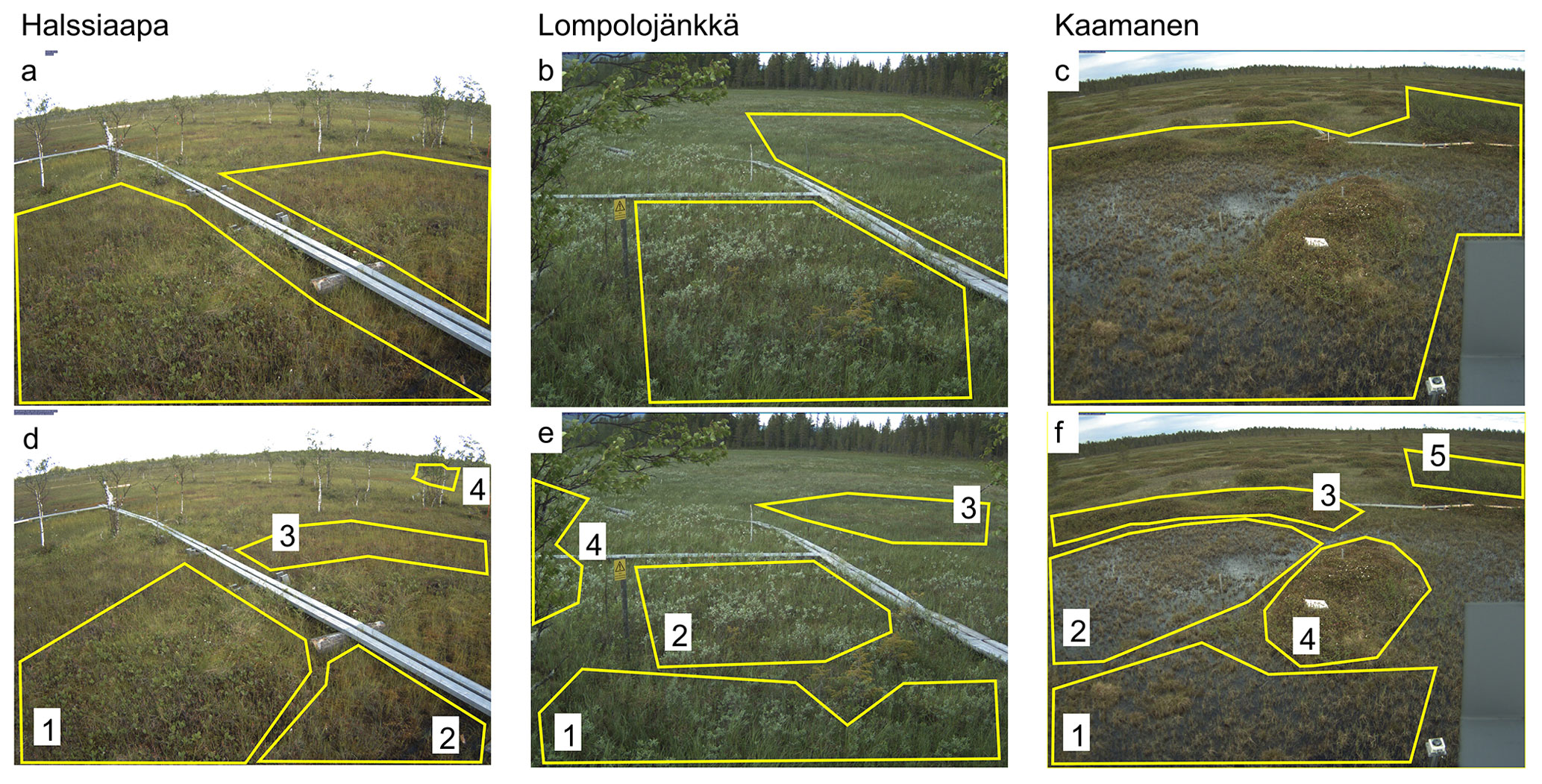
Figure 1 The regions of interest (ROIs) representing the overall vegetation at the site (a–c) and specific plant communities within the camera target areas (d–f). The numbers 1–5 indicate the plant communities detailed in Table 1.

2.3 Regions of interest (ROIs)

The ROIs covering all plant communities within the target area of the camera were defined for each site (Fig. 1a–c). In addition to these general ROIs, more specific ROIs (Fig. 1d–f) were defined for clearly identifiable plant communities characterized by specific dominant plant species (Table 1).

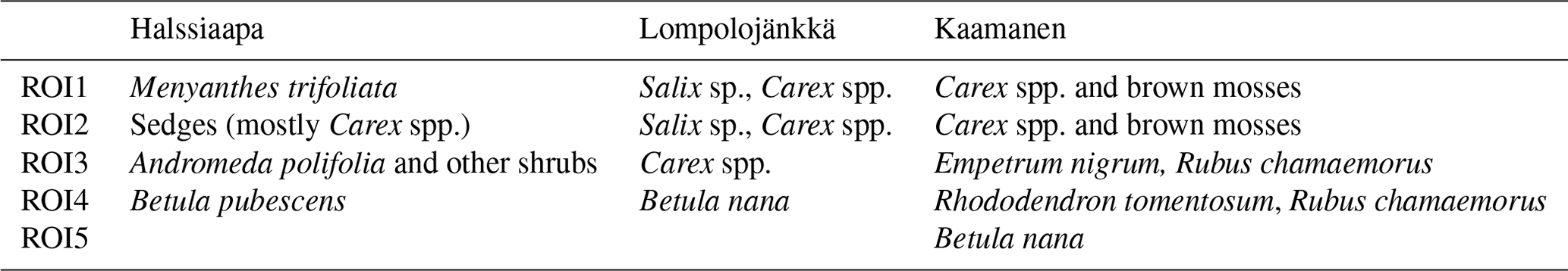
Table 1 The dominant plant species characterizing the different plant communities within regions of interest (ROIs) at each site (Fig. 1d–f).

2.4 Ecosystem-scale CO₂ exchange and meteorological observations

The ecosystem–atmosphere CO₂ exchange was measured by the micrometeorological eddy covariance (EC) method. The EC method provides continuous CO₂ flux data averaged at the ecosystem scale. The vertical CO₂ flux is defined as the covariance of the high-frequency (10 Hz) fluctuations in vertical wind speed and CO₂ mixing ratio. At each site, the EC measurement system consisted of a USA-1 (METEK GmbH, Elmshorn, Germany) three-axis sonic anemometer and a closed-path LI-7000 (LI-COR, Inc., Lincoln, NE, USA) CO₂–H₂O gas analyser. The measurement height was 6 m at Halssiaapa, 3 m at Lompolojänkkä and 5 m at Kaamanen. In addition, air temperature, photosynthetic photon flux density (PPFD) and water table level (WTD) were measured at the sites (Aurela et al., 2009).

The EC data were screened so that the flux footprint of accepted data predominantly covered the open peatland, which was the target area of measurements at each site. This screening included removing data from distinct wind direction sectors in which other ecosystems, most notably forests, contributed substantially to the measured flux. The EC systems and data processing have been presented in more detail by Aurela et al. (2001) for Kaamanen, by Aurela et al. (2015) for Lompolojänkkä and by Linkosalmi et al. (2016) for Halssiaapa. The general ROIs within the digital images were selected to coincide with the target area of the accepted EC measurements.

The measured CO₂ flux represents the net ecosystem exchange (NEE), which is the sum of gross photosynthetic production (GPP) and ecosystem respiration. The daily maximum GPP, GPP_max, was calculated as the difference between the mean daytime (PPFD>600 µmol m⁻² s⁻¹) and nighttime (PPFD<20 µmol m⁻² s⁻¹) NEE. The GPP_max describes the seasonal GPP cycle and also reacts to short-term changes in air temperature and humidity (Aurela et al., 2001).

2.5 Growing degree day sum, growing season start and temperature classes

Growing degree day sum (GDDS) was defined as the cumulative sum of the daily average temperatures exceeding 5 ^∘C, each subtracted with the base value of 5 ^∘C. The thermal growing season was considered to start when the daily mean temperature has remained over 5 ^∘C for 10 d, as defined by the Finnish Meteorological Institute (e.g. Lehtonen and Pirinen, 2019). The short-term change in GCC was expressed as a mean 3 d difference, i.e. ΔGCC = GCC(day${}_t)-\text{GCC}({\text{day}}_{t+\mathrm{3}})$. A 2 d average of these differences was calculated for each month during the growing season, and these averages were divided into three temperature classes (<5, 5–10 and >10 ^∘C). Also, cumulative GCC was calculated using the value observed just before the growing season start as the baseline. The cumulative sums were normalized by the maximum and minimum values of the year with the maximum cumulative GCC.

2.6 Satellite data

The GCC derived from the digital images of the ground-based cameras was compared with those derived from the Sentinel-2 data acquired from 2016 to 2019. GCC was computed from the atmospherically corrected bottom-of-atmosphere products (Level-2A) using bands B2 (blue, 490 nm), B3 (green, 560 nm) and B4 (red, 665 nm) with a 10 m spatial resolution. The Level-2A products were downloaded from the Copernicus Open Access Hub (https://scihub.copernicus.eu). If the Level-2A product was not available for a specific date, the Level-1C product was downloaded and processed to the Level-2A product using the Sen2Cor software (version 2.8). Cloudy, cloud-shadowed and snowy satellite images were filtered and discarded using the scene classification layer (SCL) band data available in the Level-2A products.

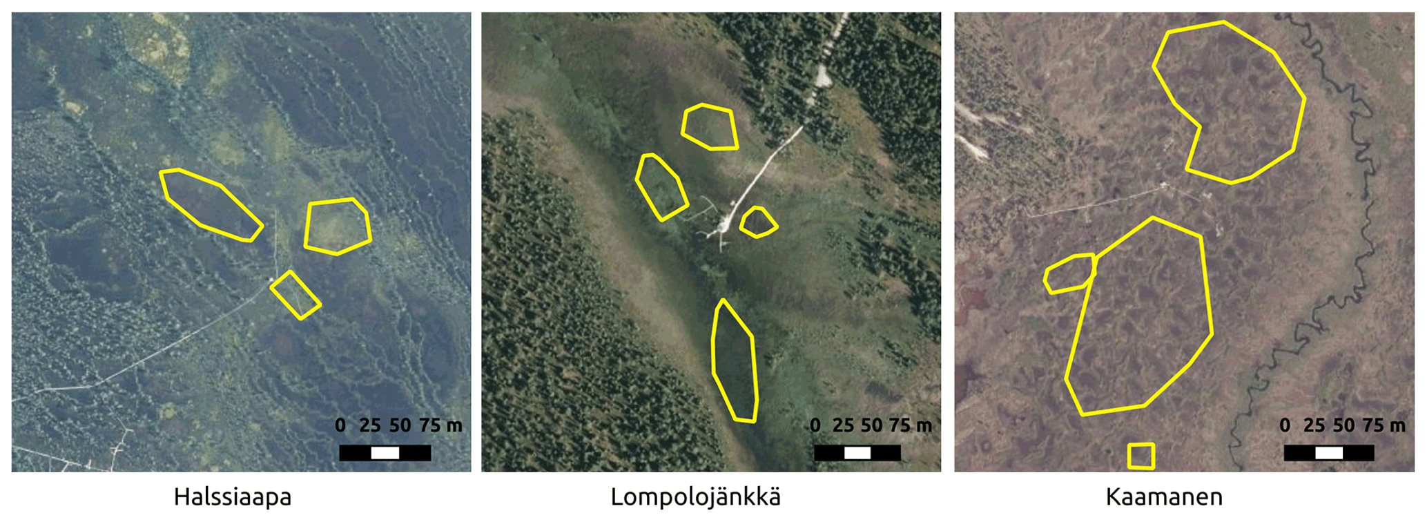
Figure 2 The regions of interest (ROIs) representing the overall vegetation at the sites for the Sentinel-2 satellite images. The aerial photo contains data from the National Land Survey of Finland Topographic Database.

GCC was calculated for multiple ROIs within each site (Fig. 2). These ROIs were different from those used with camera data because of the different spatial resolutions of the camera and satellite data. The selected ROIs represent different vegetation types with different microtopography within the study areas. The average of pixel-based GCCs within an ROI was used as the ROI-based GCC. Site-based GCC was then calculated as the average of all ROI-based GCCs within the site. The Sentinel-2 images were available at the minimum for every 2 d, due to considerable overlap between satellite orbits at the high latitudes of our study sites. Filtering out the cloud- and snow-contaminated data, however, reduced the number of valid images, which were typically available every 5 to 10 d.

2.7 Fitting of GCC and GPP_max cycles

To depict the phenology-driven seasonal cycle, we fitted a double hyperbolic tangent function to both camera- and satellite-derived GCC time series with the Levenberg–Marquardt least-squares method (Meroni et al., 2014; Vrieling et al., 2018):

$$\begin{array}{}\text{(2)}& \begin{array}{rl}& \text{GCC}\left(t\right)=a_{\mathrm{0}}+a_{\mathrm{1}}{\displaystyle \frac{\text{tanh}\left(\left(t-a_{\mathrm{2}}\right)a_{\mathrm{3}}\right)+\mathrm{1}}{\mathrm{2}}}\\ & +a_{\mathrm{4}}{\displaystyle \frac{\text{tanh}\left(\left(t-a_{\mathrm{5}}\right)a_{\mathrm{6}}\right)+\mathrm{1}}{\mathrm{2}}}-a_{\mathrm{4}},\end{array}\end{array}$$

where t is time, a₀ is the minimum GCC value at the start of the growing season, a₁ (a₄) is the difference between the maximum GCC and minimum GCC, a₂ (a₅) is the inflection point in GCC development and a₃ (a₆) controls the slope at the inflection point in GCC development during the first (second) half of the growing season. A similar function was fitted to the GPP_max data.

Visible snow included in the images affects the GCC data by overexposure. Thus, only the data collected after the snowmelt, which usually occurs in May at all sites, were used. Also, the starting point of the fits was fixed to 1 May (DOY 121, day of year), and the GCC value for this day was calculated as the average of the yearly minima after the snowmelt, whose timing was specified for each year and site. Likewise, the growing season ends by the end of October, and thus the end point of the fit was fixed to 31 October (DOY 304), for which GCC was determined by averaging the annual minima in the end of the growing season.

From the fitted function, we calculated parameters that describe phenological phases and vegetation development. These parameters were chosen as the start of season, SOS25, which stands for 25 % of the GCC difference between the maximum and 1 May; maximum GCC, Max; and the end of season, EOS25, defined as 25 % of the GCC difference between 30 October and the maximum. The thresholds are in accordance with Richardson et al. (2019) and were chosen to minimize the disturbance of excess surface water after the snowmelt.

2.8 Statistical analysis

The differences in GCC between the sites, different plant communities and measurement years were tested with the Kruskal–Wallis one-way analysis of variance on ranks for the groupwise comparison. Dunn's test was used for post hoc testing, and the significance values were adjusted by the Holm correction for multiple tests. The Kruskal–Wallis method was used due to the non-normal distribution of the seasonal GCC data. The presence of autocorrelation in the residuals of the regression between GCC and GPP_max was verified with the Durbin–Watson test. Autocorrelation was taken into account by regressing the first differences in the data, i.e. by applying the transformation ${x^{\prime }}_t=x_t-x_{t-\mathrm{1}}$, where x_t and x_t−1 are consecutive observations. The statistical analyses were performed with the R software (version 4.2.0).

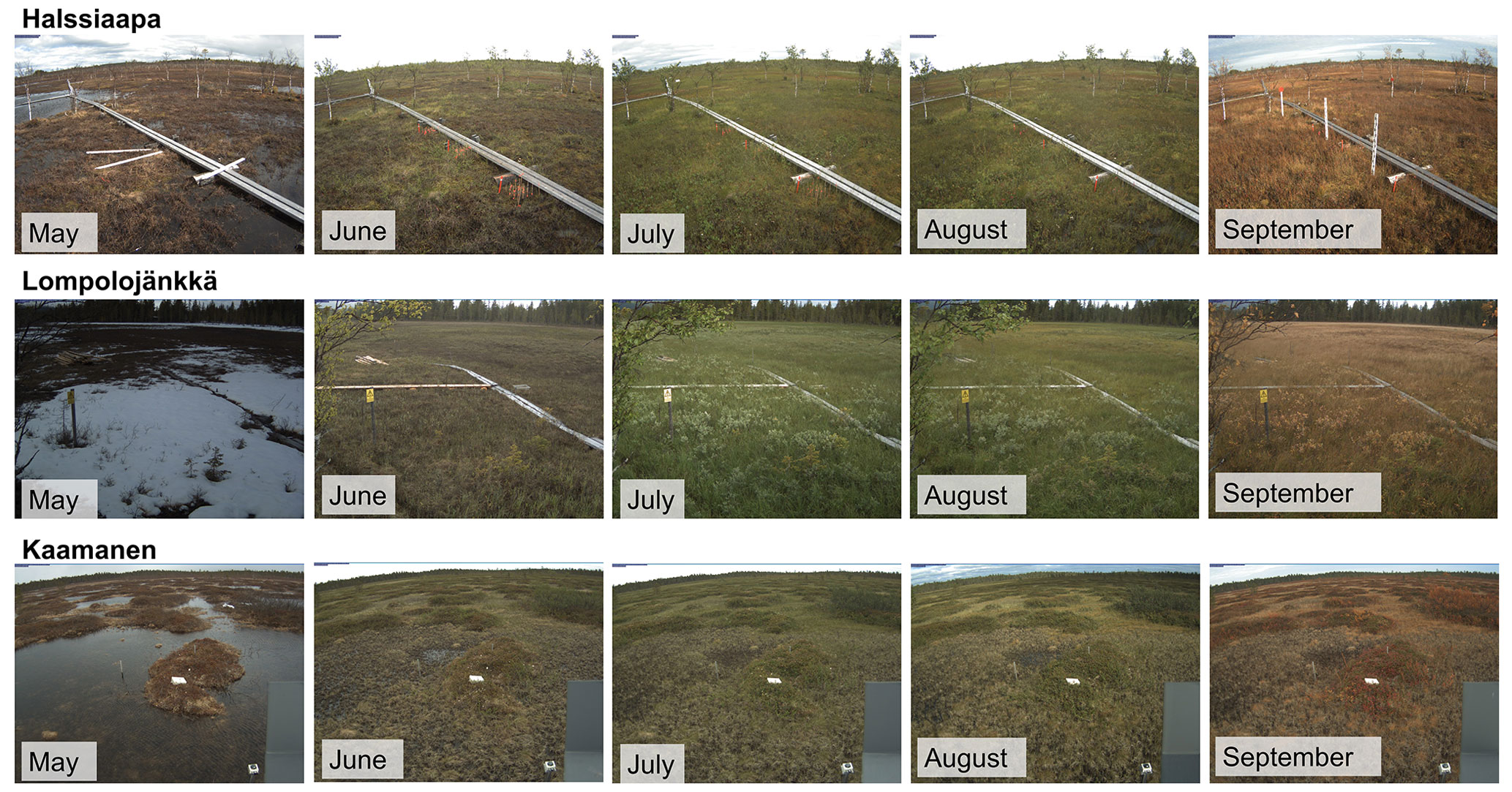
Figure 3 The seasonal development of vegetation and surface water from May to September in 2015 at Halssiaapa, Lompolojänkkä and Kaamanen. The pictures were taken on the 15th of each month.

3 Results

3.1 Greenness variation

The seasonal development of vegetation during the growing season could be visually observed from the imagery collected at our study sites, as exemplified by Fig. 3. The spring development, greening and senescence of vegetation during the growing season were visible in the images, as were the changes in the areas covered by surface water.

The mean growing season GCC values obtained from the phenological cameras showed that Lompolojänkkä systematically had the highest GCC values over the five growing seasons (Figs. 4, S4–S6). The Kruskal–Wallis groupwise statistical test showed significant difference between the sites during all the measurement years (Table 2). In 2015, 2016 and 2018, there was a significant difference in GCC between Lompolojänkkä and the other two sites according to the pairwise statistical analysis (Table S2). In 2017, 2018 and 2019, the pairwise comparison showed a significant difference in GCC between Halssiaapa and the other two sites (Table S2). The maximum GCC during the whole study period of 2015–2019 was observed in 2017 at Lompolojänkkä and Kaamanen and in 2016 at Halssiaapa (Fig. 4, Table 3).

Table 2 The significant differences in GCC between the sites during the measurement years as a groupwise comparison (Kruskal–Wallis one-way analysis of variance on ranks). χ² denotes the chi-squared test statistic.

Figure 4 Daily camera-based GCC values from 1 May to 30 September in 2015–2019.

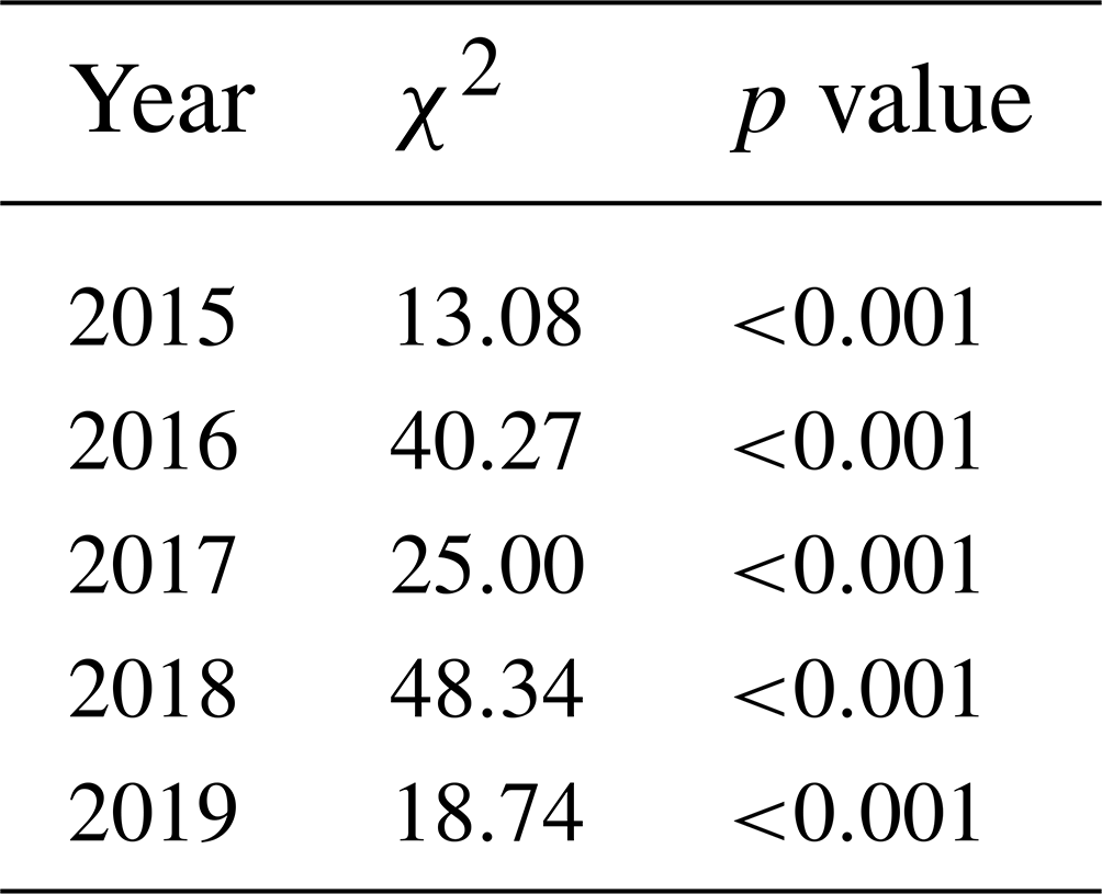
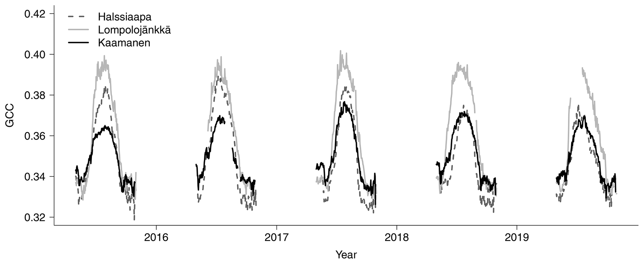
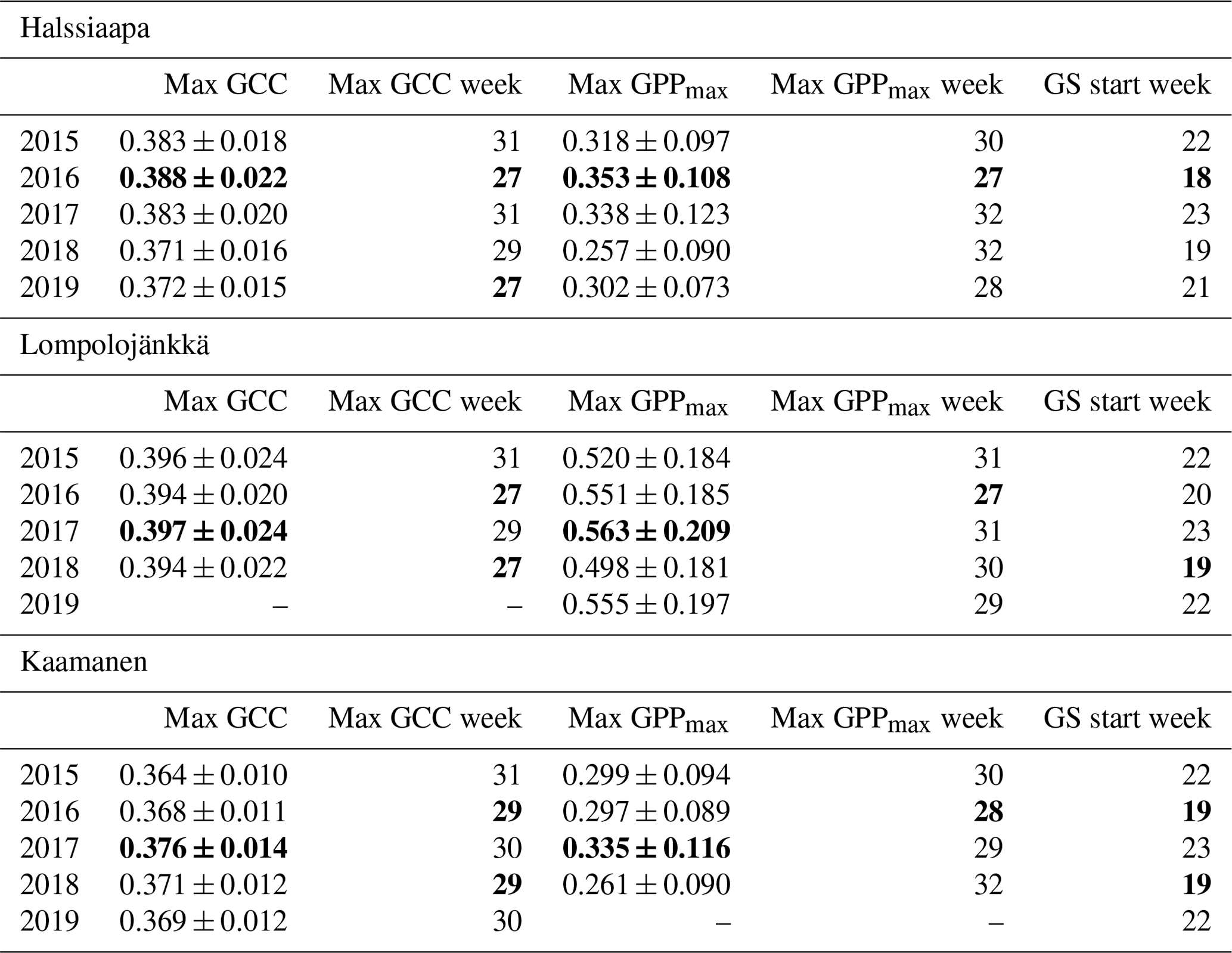
Table 3 The mean GCC and GPP_max (mg CO₂ m⁻² s⁻¹) during the week they attained the maximum, the week numbers of these maxima and the week number of the growing season (GS) start. The maximum GCC and GPP_max, the earliest maximum GCC and GPP_max and the earliest GS start are marked as bold. The maximum GCC data at Lompolojänkkä and maximum GPP_max data at Kaamanen are not reported for 2019 due to data gaps.

There were significant GCC differences among different plant communities at all sites (p<0.05), except in 2017 at Halssiaapa and Kaamanen (Tables S3 and S4). In general, at all sites the GCC of birch species (Betula pubescens and B. nana) differed significantly from the other plant species. At Halssiaapa, the plant communities with sedges (Carex spp.) and shrubs (e.g. Andromeda polifolia) differed from annuals with bigger leaves, such as Menyanthes trifoliata. At Kaamanen, the shrubs and annuals (e.g. Empetrum nigrum, Rhododendron tomentosum, Rubus chamaemorus) had a significantly higher GCC than the plant communities with sedges and brown mosses. The comparison of the maximum GCC values of different plant communities, calculated as weekly means, supported these results, as the annuals and woody plants with relatively large leaves, such as M. trifoliata, R. chamaemorus, Salix sp. and Betula spp., generated a higher GCC maximum than Carex spp. and shrubs (Table 4). At Halssiaapa, the highest maximum GCC during 2015–2017 and 2019 was observed in ROI1, which is dominated by M. trifoliata, whereas in 2018 the highest GCC was found for ROI3, an area with A. polifolia and other shrubs. At Lompolojänkkä, the highest annual GCC maximum was consistently observed in a plant community dominated by Salix sp. and Carex spp. (ROI1). Most likely the ground layer with mosses and dead plant material reduced the GCC within those ROIs that had sparse vegetation. Among the measurement years, most plant communities at Halssiaapa showed the highest maximum GCC in 2016. At Lompolojänkkä, the maximum GCC of different ROIs varied between the years 2015, 2016 and 2017, while at Kaamanen all plant communities attained their maxima in 2017.

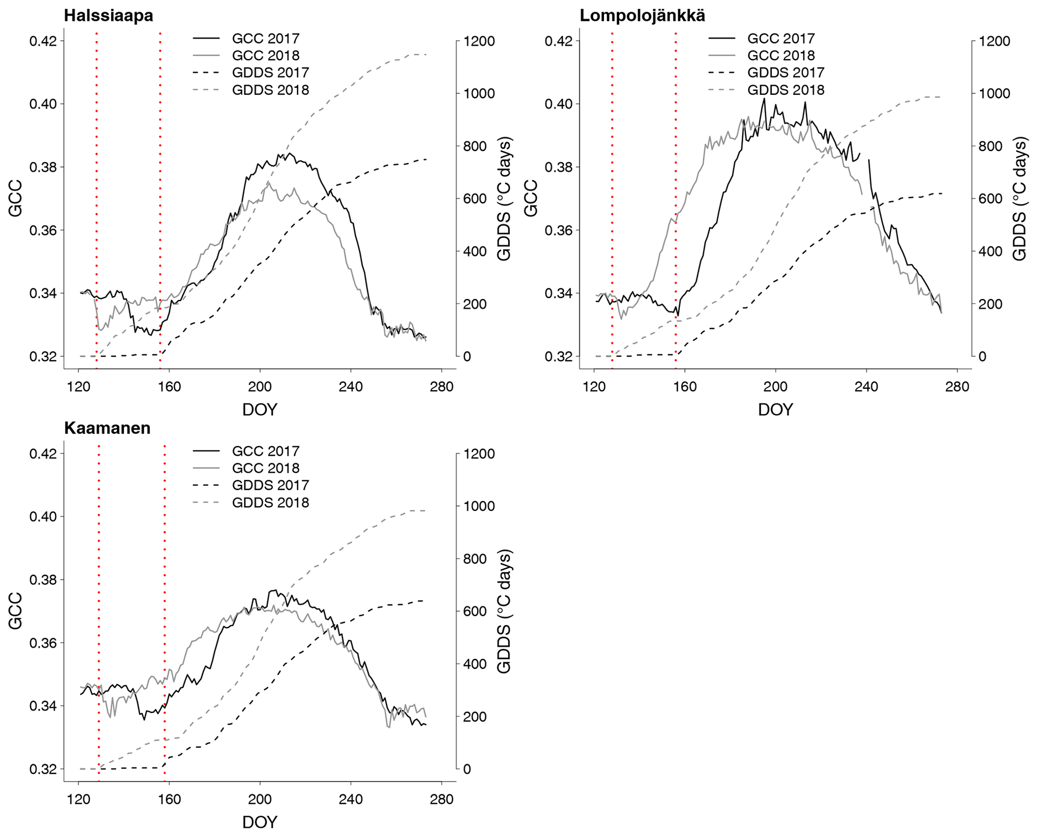
Figure 5 Development of GCC and growing degree day sum (GDDS) from 1 May to 30 September at Halssiaapa, Lompolojänkkä and Kaamanen. The years 2017 and 2018 are shown here as an example of a cold and warm spring, respectively. The grey dashed lines indicate the start of the growing season.

3.2 Temperature and GCC development

The relationship between temperature and GCC was examined by creating normalized cumulative GCC and GDDS curves for all the growing seasons (Figs. S4–S6). These show that the GCC started to accumulate later than GDDS. In 2017, the snow cover lasted at all sites until the beginning of June, which delayed the GDDS development and the start of the growing season compared to the other study years (Figs. 5, 7, 8, 9 and S3–S6). Consequently, GCC did not increase until the beginning of June (4 June in Halssiaapa and Lompolojänkkä and 7 June in Kaamanen), when the snow was melted. Despite the slow start of growth in 2017, the peatland vegetation was capable of catching up its typical development, and at Lompolojänkkä and Kaamanen GCC even reached the highest summer maximum during the study years (Table 3).

During the measurement years, warmer springs and thus earlier snowmelts resulted in an earlier green-up of vegetation. No clear connection between the growing season start and the timing of the maximum of either GCC or GPP_max was found at Lompolojänkkä or Kaamanen (Table 3). At Halssiaapa, however, the earliest growing season start, the maximum value and the earliest timing of both GCC and GPP_max occurred in the same year, 2016. During our study period, the year 2018 had the warmest summer at all sites (Fig. S3). July 2018 had the highest mean air temperature among the measurement years, which was also higher than the mean temperature of the period 1981–2010 (Table S1). The high temperatures and low precipitation resulted in drought, which was observed as a WTD drop at Halssiaapa and Kaamanen (Figs. S2 and Table S1). June 2018 was average in terms of meteorological conditions, but the mean air temperatures during the measurement years were highest in 2018 (Table S1). At Halssiaapa, the WTD increased substantially during the growing seasons of 2018 and similarly in 2019 as a result of the drought (Fig. S2). The same was true at Kaamanen (data missing in 2019), while at Lompolojänkkä WTD was not affected. The effect of drought is also visible in the daily and cumulative GCC values (Figs. 4 and S4–S6).

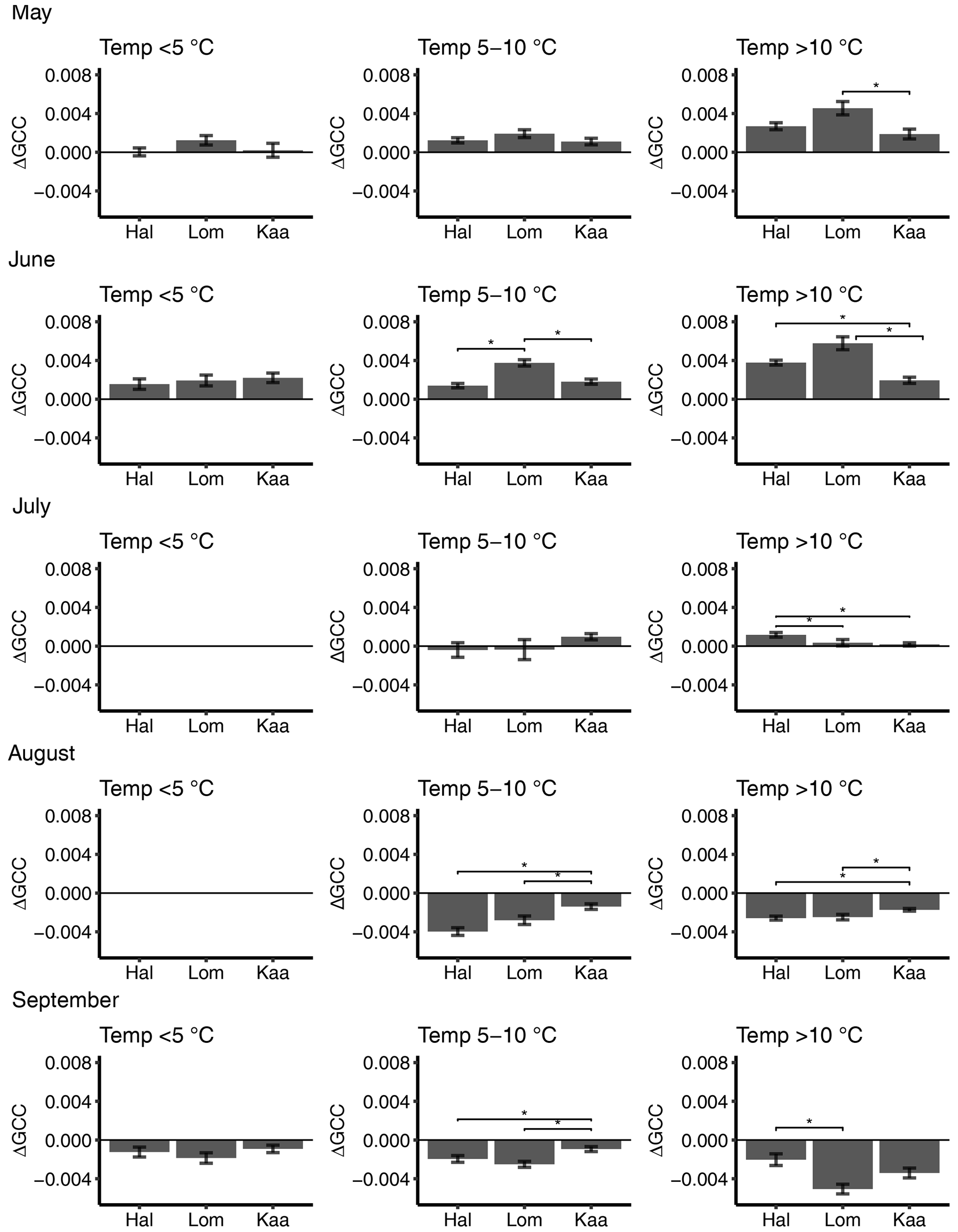
Figure 6 Mean 3 d difference in GCC divided into temperature classes (<5, 5–10, >10 ^∘C) at Halssiaapa (Hal), Lompolojänkkä (Lom) and Kaamanen (Kaa) from May to September. There are no temperature data in the <5 ^∘C class in July and August. The error bars denote the standard error, and the asterisks denote the statistically significant (p<0.05) difference between the sites.

The short-term (3 d) change in GCC, ΔGCC, which is indicative of vegetation development in different temperature classes, depended on both the month and temperature range (Fig. 6). In May, ΔGCC was substantially smaller for temperatures below 5 ^∘C than above 5 ^∘C. Significant differences were found neither between the sites nor during any month in the lowest temperature class (Fig. 6, Table S5). At Lompolojänkkä, ΔGCC was generally larger than at the other sites. The vegetation growth in June at Halssiaapa seemed to benefit from temperatures over 10 ^∘C, while at Lompolojänkkä this limit was lower. At Kaamanen, however, the ΔGCC in June was similar in all temperature classes. In July, GCC started to stabilize, and a significant positive change was only observed at Kaamanen for temperatures between 5 and 10 ^∘C and at Halssiaapa for temperatures over 10 ^∘C. In August and September, ΔGCC was negative due to senescence (Fig. 6). The results of statistical pairwise comparisons and significant differences between the sites are shown in Table S6.

The ΔGCC of different plant communities (Figs. S7–S9) showed that the growth of Betula spp. started strong in May at all sites, but in June the birches already had a lower ΔGCC than other plant communities. The highest plant community-specific ΔGCC values were found at Lompolojänkkä, which was consistent with the spatially averaged ΔGCC data (Figs. 4 and 6).

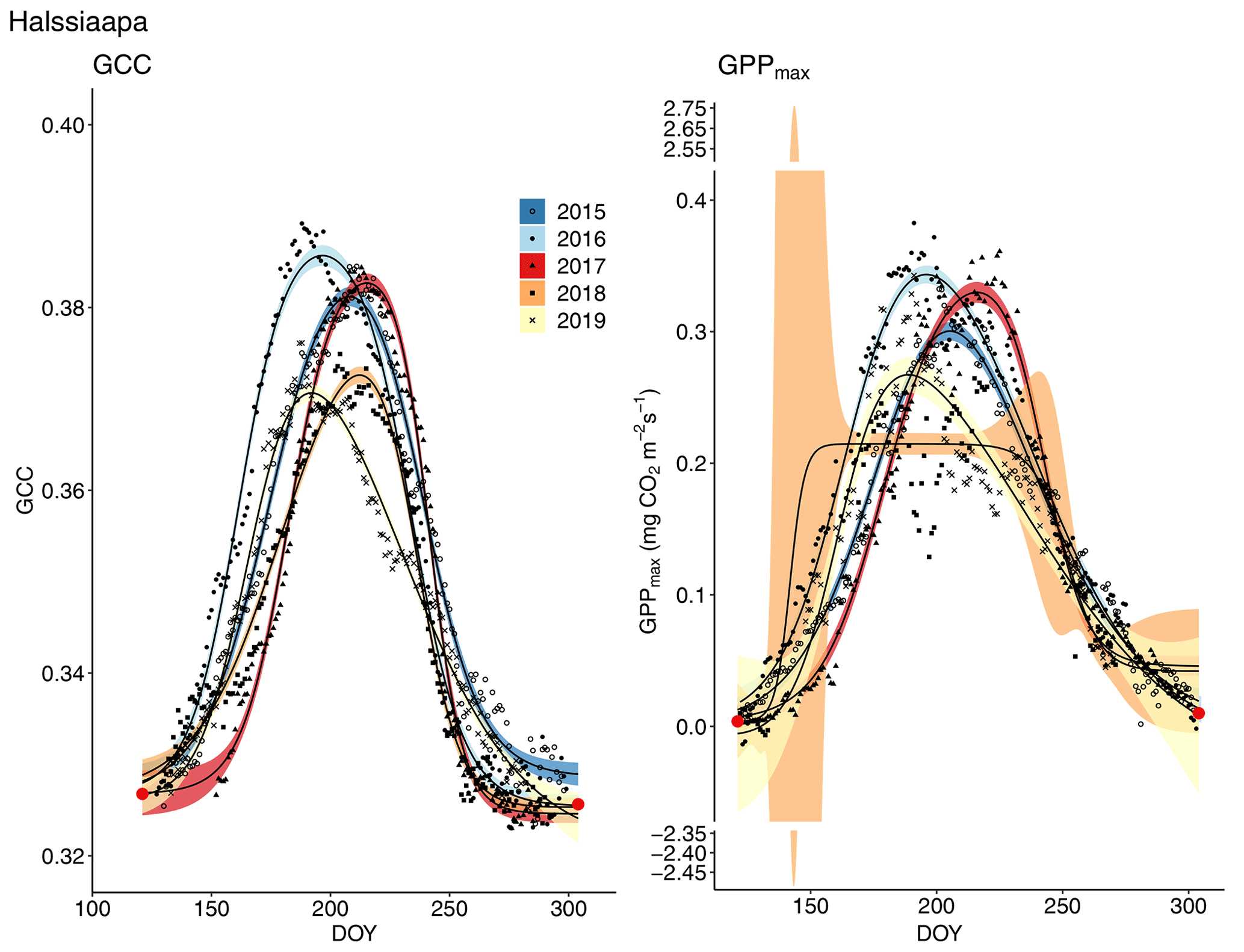
Figure 7 Development of GCC and GPP_max from 1 May to 30 September in 2015–2019 at Halssiaapa. Different symbols and colours denote different years, and the bands show the 95 % confidence intervals of the fitted double hyperbolic tangent function. The red dots indicate the fixed start and end days defined for the fitting.

3.3 Seasonal GCC and GPP_max development

The start and end of the growing season were clearly visible in both the GCC and GPP_max data, which showed the same seasonal pattern (Figs. 7, 8 and 9). As mentioned above, in 2017 the snow cover lasted until the beginning of June, which delayed the start of photosynthesis and thus vegetation development. At Halssiaapa, the year 2018 was hot and dry compared to the other measurement years and the long-term average (Fig. S2 and Table S1), and this was reflected in the GCC and GPP_max data that were lower than in other years (Fig. 7). In addition, the GPP_max data were sparse during the growing season of 2018 at Halssiaapa, which impaired the fit and resulted in a wider confidence interval (Fig. 7). During the study period, the highest values of both GCC and GPP_max were observed in 2016 at Halssiaapa and in 2017 at Kaamanen and Lompolojänkkä (Figs. 7, 8 and 9). In general, Lompolojänkkä had the highest GPP_max, GCC and LAI (Figs. 4, 7, 8 and 9).

The difference in GCC was significant (p<0.05) between Lompolojänkkä and the other two sites in 2015, 2016 and 2018 (Table S2). The difference in GCC between Halssiaapa and other sites was significant in years 2017, 2018 and 2019 (Table S2). In 2017, GPP_max showed no statistical difference among the sites (Table S7). In 2016 and 2019 there was a significant difference (p<0.05) between Kaamanen and the other two sites, as well as in 2015 and 2018 between Lompolojänkkä and Kaamanen (Table S8). The GPP_max and GCC showed a similar course throughout the growing season (Figs. S19, S20 and S21).

Table 4 The maximum GCC values of different plant communities characterized by the dominant species specified in Table 1 (defined as image ROIs) from 2015 to 2019. The maximum value among different ROIs is marked as bold, and the maximum among the years is italic. The values marked as bold and italic describe the value being both maximum among the ROIs as well as the measurement years. The ROIs are described in Sect. 2.4. The data from Lompolojänkkä are missing in 2019.

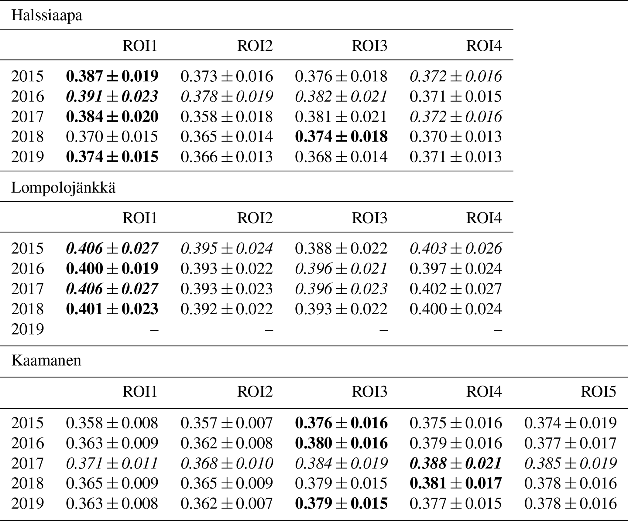
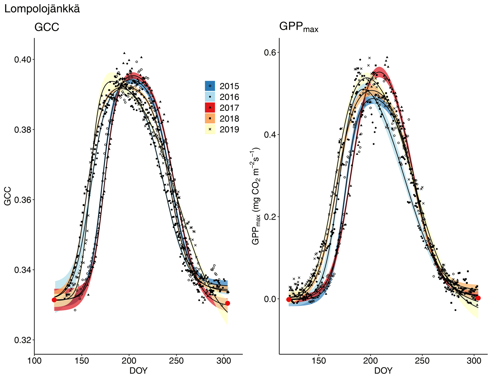
Figure 8 Development of GCC and GPP_max from 1 May to 30 September in 2015–2019 at Lompolojänkkä. Different symbols and colours denote different years, and the bands show the 95 % confidence intervals of the fitted double hyperbolic tangent function. The red dots indicate the fixed start and end days defined for the fitting.

Table 5 The coefficient of determination (R²) of the linear regression between GCC and GPP_max and of the regression after differencing the data for autocorrelation.

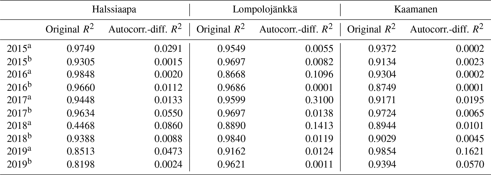
^a Period before the annual GCC maximum. ^b Period after the annual GCC maximum.

A linear relationship between GCC and GPP_max was observed during both the increasing and decreasing phases of GCC (Table 5, Figs. S16–S18). The coefficient of determination (R²) of the original linear regression for the first phase of 2018 at Halssiaapa was low due to a gap in the GPP_max data and the hot and dry weather conditions that temporarily reduced GPP_max. However, the Durbin–Watson test indicated that there was significant and strong autocorrelation in the model residuals. After differencing the data, the coefficient of determination was generally close to zero. There were periods showing correlated short-term variation in GCC and GPP_max, for example, at Kaamanen from late May to mid-June in 2016 and in June 2017 (Fig. S21), but most of the common variation in GPP_max and GCC was associated with the common seasonal cycle (Table 5).

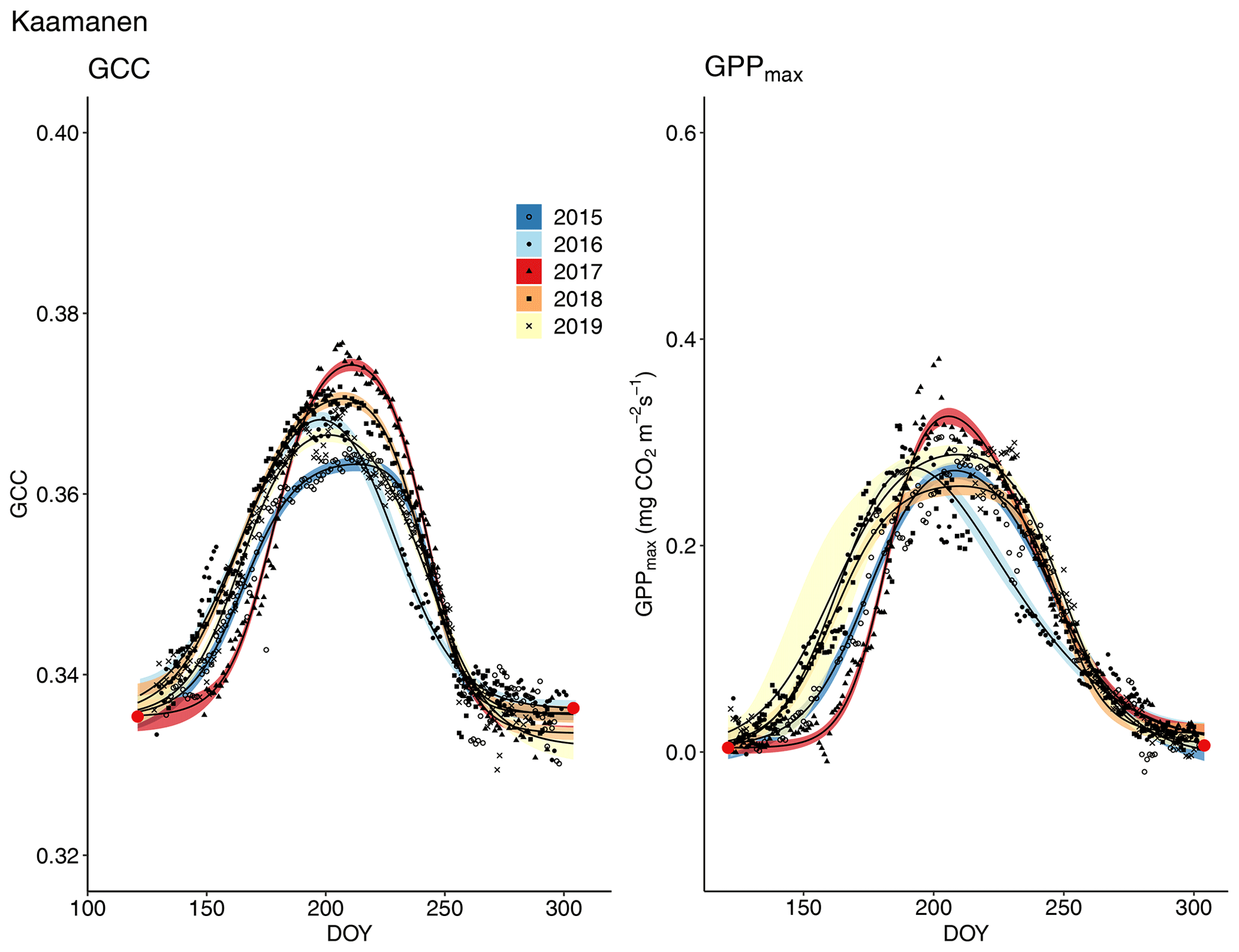
Figure 9 Development of GCC and GPP_max from 1 May to 30 September in 2015–2019 at Kaamanen. Different symbols and colours denote different years, and the bands show the 95 % confidence intervals of the fitted double hyperbolic tangent function. The red dots indicate the fixed start and end days defined for the fitting.

3.4 Comparison between digital-camera- and satellite-derived GCC

The GCC retrieved from the Sentinel-2 images had the same seasonal pattern as the camera-derived GCC (Fig. 10). Due to the sparseness of satellite data, however, the uncertainties were greater, as shown by the wider confidence intervals. The later season start and GCC maximum in 2017 at all sites and the lower GCC at Halssiaapa in 2018, compared to the other measurement years that were observed with cameras, were visible in the satellite-derived GCC. The GCC values from Sentinel-2 were in general higher than the camera-based GCC, which is most probably due to the different viewing angles and atmospheric effect (the scattering and absorption of radiation due to atmospheric molecules and aerosols) and the consequent atmospheric correction of the satellite data.

Table 6 Growing season phases estimated from camera and satellite images (DOY): SOS25 (start of season, 25 % difference between start and maximum), Max (maximum GCC) and EOS (end of season, 25 % difference between end and maximum).

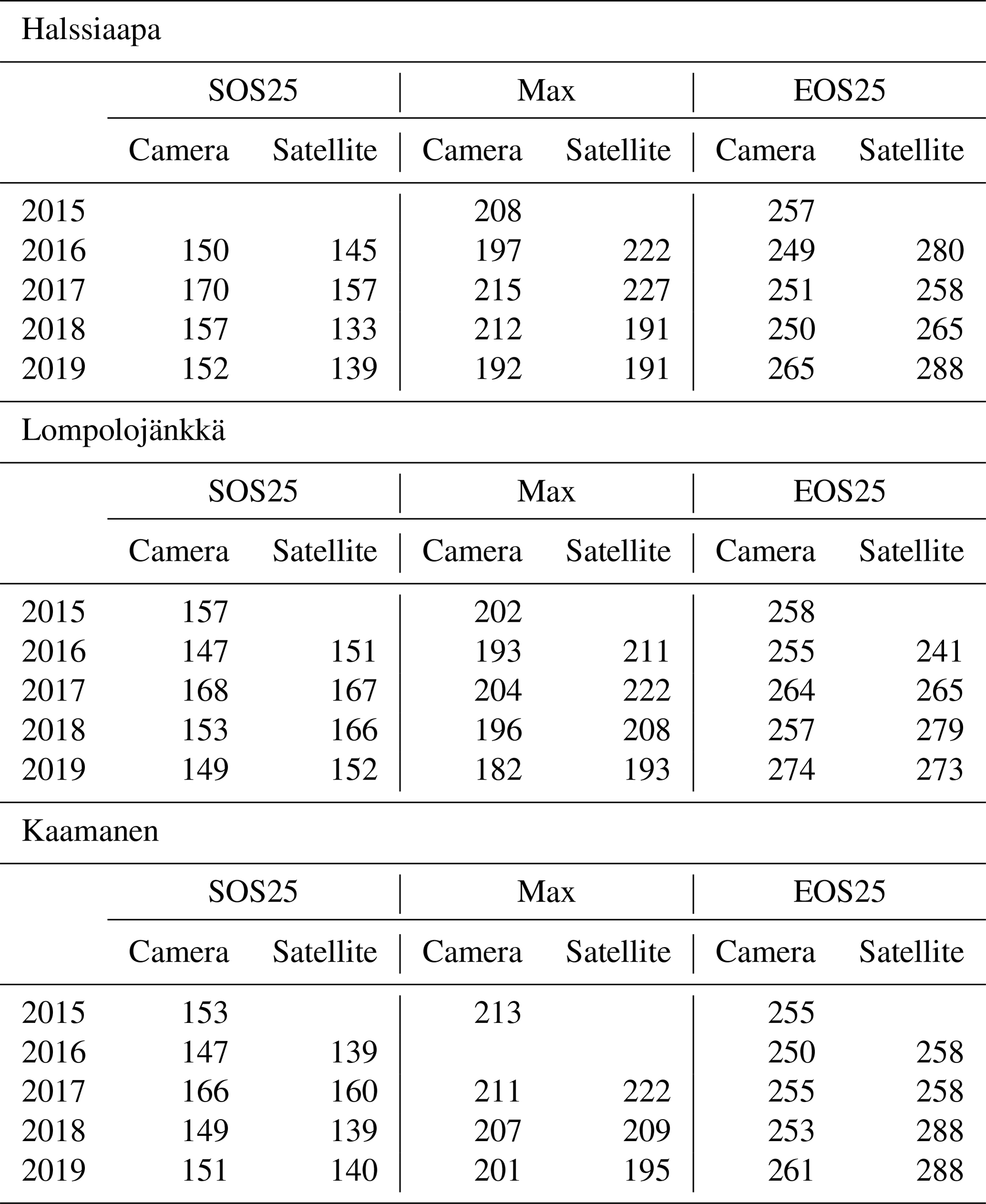
The estimated parameters describing different growing season phases, which were calculated from the fitted models, Eq. (2), show substantial differences between satellite and camera data (Table 6). At Halssiaapa and Kaamanen, the season start (SOS25) was estimated to start earlier based on the Sentinel-2 data, whereas at Lompolojänkkä the timing of SOS25 and Max occurred later. The timing of the end of season (EOS25) was estimated later with the Sentinel-2 data at Halssiaapa and Kaamanen, while at Lompolojänkkä there was no systematic difference.

4 Discussion

In this study, we examined how vegetation phenology, here described with GCC, varied in three natural peatlands in northern Finland during five growing seasons and how it depends on the site-specific characteristics and the composition of vegetation. The collected data allowed us to create a continuous representation of the development of greenness, which could be related to observed changes in the ecosystem–atmosphere flux of CO₂ and compared with the corresponding satellite-derived data.

We found the highest GCC values at Lompolojänkkä, a fen with high nutrient availability, rich vegetation and the highest LAI of the study sites (Fig. 4). The highest GCC also coincided with the highest photosynthetic productivity at peak summer. At Lompolojänkkä, the surface is flatter than at the other sites; at Halssiaapa and Kaamanen the pronounced microtopography results in a higher variability in the hydrological features and consequently in the trophic status and vegetation. Also, the stream running through Lompolojänkkä feeds water and nutrients to its surroundings (Lohila et al., 2010; Aurela et al., 2009). This affects the site's nutrient status and is reflected in vegetation, which mainly consists of annuals such as Carex spp. and Menyanthes trifoliata, and thus in the magnitude of GCC and GPP_max reported here.

Related to the microtopographical differences between the study sites, we found a higher GCC in those plant community types that had annuals and taller woody plants with bigger leaves (e.g. Menyanthes trifoliata, Rubus chamaemorus, Salix sp., Betula spp.) and, correspondingly, a lower GCC in areas dominated by sedges (e.g. Carex spp.) and smaller shrubs (e.g. Empetrum nigrum, Rhododendron tomentosum, Andromeda polifolia) and mosses (Table 4, Fig. S1 in the Supplement). At Kaamanen, however, the shrubs (E. nigrum, R. tomentosum) showed higher GCC than the sedges and mosses. The different plant communities also have different habitats. For example, shrubs thrive in drier locations such as strings, while many annuals (e.g. sedges, Menyanthes trifoliata) favour wetter environment.

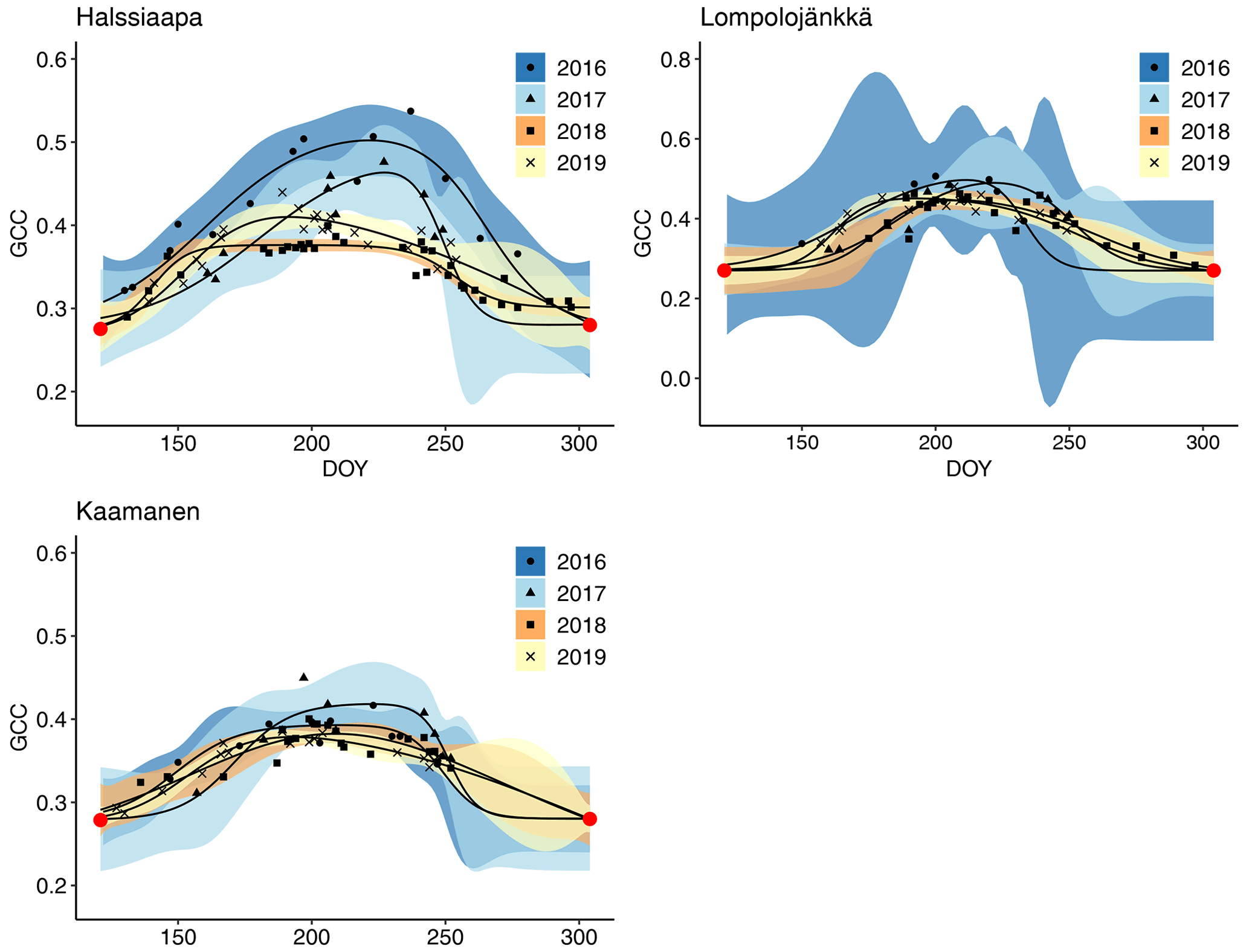
Figure 10 Mean GCC derived from the Sentinel-2 data from 1 May to 30 September in 2016–2019 at Halssiaapa, Lompolojänkkä and Kaamanen. Different symbols and colours denote different years, and the bands show the 95 % confidence intervals of the fitted double hyperbolic tangent function. The red dots indicate the fixed start and end days defined for the fitting. Note the different y-axis scaling for Lompolojänkkä.

Compared to traditional and more laborious measurements of vegetation phenology, the digital-camera-based measurements automatically produce high-frequency data in an effortless way. Even though the variation in GCC among the sites was greater than the variation among the ROIs within one site, our results indicate that vegetation monitoring is feasible even at the plant community level. Comparative studies on the greenness of different plant communities or small ROIs within a digital camera image are still sparse. For example, Davidson et al. (2021) studied the phenology of different boreal peatland vegetation (defined as bog and fen) at the chamber plot scale (<0.5 m²), while Menzel et al. (2015) and Cheng et al. (2020) derived vegetation indices from digital images at the scale of individual trees. These kinds of GCC observations of the differentially developing vegetation types have a potential to help in partitioning an integrated CO₂ flux observation into components allocated to these vegetation types. Different ecosystems, plant communities and species may respond differently to changes in environmental conditions, such as warm spells and timing of the growing season start, depending on their characteristics and habitats.

With regard to timing, a warm spring very likely leads to an earlier growing season start. Nevertheless, our data show that even though the growing season start was late at the study sites in 2017 due to a cold spring and late snowmelt, vegetation was capable of reaching the same maximum GCC level as in other years, and at Lompolojänkkä and Kaamanen vegetation it even attained the 5-year GCC and GPP_max maximum (Figs. 8 and 9, Table 3). A review by Wipf and Rixen (2010) on arctic and alpine ecosystems concluded that a delayed snowmelt and thus a shorter growing season decreases the overall plant productivity of an ecosystem, but it also noted that the effect of snowmelt timing depends on the plant functional type; for example, the growth of forbs increases, while the growth of grasses decreases when the snowmelt occurs later. The later phenological phases are most likely controlled by GDDS rather than the timing of the growing season start (Wipf, 2010). Furthermore, the phenology of plant species that usually start developing earlier after the snowmelt and the first phenological phases of all plant species are more sensitive to changes in the snowmelt timing. Our results imply that the northern peatland vegetation is capable of quick growth following a cold spring, and the vegetation can even increase gross primary production if the conditions are favourable later during the growing season, as was the case in 2017. This was clearly observed in the magnitude and timing of the maximum GCC. The faster GCC increase and lower temperature sensitivity at Lompolojänkkä than at the other sites are explained by the nutrient status of this fen.

As observed in several studies conducted in different ecosystems (forests, grasslands, crops, peatlands), GPP correlates strongly with the greenness index derived from digital camera images (Richardson et al., 2008; Migliavacca et al., 2011; Keenan et al., 2014; Peichl et al., 2015; Toomey et al., 2015; Linkosalmi et al., 2016; Knox et al., 2017; Järveoja et al., 2018; Peichl et al., 2018; Koebsch et al., 2019). Our results agree with these studies, showing highly similar seasonal cycles of GCC and GPP_max at open peatlands dominated by shrubs and deciduous plants. Essentially, both are controlled by the amount of green leaf area, which in turn is driven mainly by temperature and day length (Bauerle et al., 2012; Peichl et al., 2015; Koebsch et al., 2019). When temperature increases, the plant chemical reaction rates also increase, triggering photosynthesis (Bonan, 2015). According to our results, air temperature, expressed here as a degree day sum (Fig. 5), explained well the annual differences in the early phase of the growing season, which has also been previously observed for a more southern boreal peatland (Peichl et al., 2015). In the latter part of the growing season, the decreasing day length and temperatures strongly drive the gradual degradation of chlorophyll content, which eventually leads to downregulation of photosynthesis and further to leaf fall and winter dormancy (Larcher, 2003; Öquist and Huner, 2003; Bonan, 2015).

The camera-derived GCC data depicted the differences in the phenological development between the measurement years and the variation in the maximum greenness level among the years and sites and in relation to GPP_max could be assessed from the GCC data. Lompolojänkkä showed significantly higher maximum GCC and GPP_max than the other sites during all the years (Fig. 8, Table 3). Also, the maximum GCC and GPP_max were found in the same year at all sites. In addition to the seasonal cycles, GCC and GPP_max show distinct periods of correlated short-term variation, which is mainly controlled by abiotic factors, such as temperature and solar radiation (Peichl et al., 2015). For example, the variation in GCC and GPP_max was highly similar during the first part of the growing seasons of 2016 and 2017 at Kaamanen (Fig. S21) and during the drought period in 2018 at Halssiaapa (Figs. 7, S19). At Lompolojänkkä, this widespread drought did not result in a WTD decrease (Fig. S2), which was due to the local hydrological features, and the net CO₂ uptake even increased in contrast to other northern sites (Rinne et al., 2010). At Kaamanen, however, the drought decreased the CO₂ sink, counterbalancing the gain due to the earlier growing season start in 2018 (Heiskanen et al., 2021). Our data show that the drought in 2018 and 2019, observed in WTD and air temperature data (Fig. S2 and Table S1), affected the CO₂ sink most at Halssiaapa (Figs. 7, S13). The greenness data, both from the Sentinel-2 satellite and digital photography, are in good accord with these observations of CO₂ flux dynamics (Figs. 7–10). Despite the specific periods of correlation, our regression analysis indicates that most of the variation in GPP_max can be explained by the common seasonal cycle rather than the short-term variations in GCC (Table 5).

The fitting of a hyperbolic tangent function to GCC data to characterize the basic phenological cycle worked well when data availability was sufficient (Figs. 7, 8, 9 and 10). The effect of poor data coverage is especially evident in the Sentinel-2 data in the beginning and end of the growing season, as well as when the camera or the GPP_max data were limited, such as in the early growing season at Halssiaapa in 2018 and at Kaamanen in 2019, resulting in wide confidence intervals of the fit (Figs. 7–10). Such data losses obviously compromise the accurate timing of the phenological phases. We also found large differences between the camera- and satellite-derived growing season phases (Table 6), with the fits to the Sentinel-2 data suggesting a longer growing season at Halssiaapa and Kaamanen. Nevertheless, the main phenological changes during the growing season were visible also in the satellite data. Vrieling et al. (2018) found large differences between the phenological parameters derived from the satellite-based NDVI (normalized difference vegetation index) and camera-based GCC time series, especially in the end of the growing season. They suggested that differences could be explained by the non-photosynthetic vegetation mass, such as dead plant matter, stems and flowers, which in an oblique view affects the visibility of the green plant mass in the image. Thus, Vrieling et al. (2018) proposed that camera observations taken at nadir, rather than from an oblique view, could produce better correlation between satellite and camera data. Also, it should be noted that the satellite indices are estimated from surface reflectance, while the camera image analysis applies raw digital numbers that scale with the reflected radiance (Vrieling et al., 2018). Thus, the resulting GCC estimates can be expected to differ between the techniques, as also observed in the present study.

Obviously, the temporal coverage of satellite data, typically including non-cloudy image every 5 to 10 d for our study sites, is limited compared to the high-frequency camera-based measurements. The satellite data were limited especially during 2016 and 2017, because at that time Sentinel-2 constellation consisted only of Sentinel-2A. Since 2018, however, there have been data available from two satellites (Sentinel-2A and Sentinel-2B). Overall, mapping the vegetation on these heterogeneous peatlands with remote sensing methods is challenging, and the suitability of the methods depends on the peatland structure (Räsänen et al., 2019). By providing local, continuous data even on the plant community level, digital photography could be used for verification of remote sensing products and as supporting information for their interpretation, as well as for filling the gaps in the landscape-level data (Filippa et al., 2018; Richardson et al., 2007, 2009; Sonnentag et al., 2012). The applicability of satellite-based remote sensing in tracking vegetation phenology can be improved by increasing the temporal resolution by combining multiple satellite data sources and using data from satellite constellations with very high temporal resolution such as PlanetScope (Cheng et al., 2020; Wand et al., 2020).

5 Conclusions

In this study, we showed that the digital-photography-derived greenness index (GCC) differed between three northern boreal peatland sites, with the differences being associated with nutrient availability and LAI. At all sites, the seasonal course of GCC was closely correlated with that of CO₂ uptake. The digital images also enabled determining the GCC of different plant communities, suggesting that these images can potentially be used for partitioning the ecosystem-scale CO₂ flux measurement. The spring temperatures and consequent variation in growing season start affected the daily GCC and maximum gross photosynthetic production (GPP_max), but the peatland vegetation showed capability to compensate for a late start and even to reach the maximum GPP_max observed during the 5 study years. The effect of drought on GCC and GPP_max depends on local hydrological features and thus the drought resistance of the site, which indicates the possible effects of climate warming and more frequent droughts. Despite the seasonal coherence between the GCC and CO₂ uptake data, the short-term variation in GCC did not in general explain the corresponding variation in GPP_max.

The remote sensing (Sentinel-2) data were consistent with the camera-based data, but better temporal resolution would be needed for a more reliable timing of different phenological phases. From our analysis of the camera-based results, we can conclude that the chromatic data obtained from digital cameras provide an effective and reliable measurement of vegetation greenness. These observations on vegetation phenology serve as a means of continuous monitoring and understanding the shifts in vegetation due to land use and climate change, even on a plant community scale. Time-lapse imaging was here employed in parallel with continuous, ecosystem-scale CO₂ flux measurements, but focused on a small spatial scale it is likely to provide substantial support to non-continuous, chamber-based flux measurements as well. Also, ecosystem modelling could benefit from the parameterization of phenological events based on camera data and the use of these data for model evaluation. Furthermore, these results provide input for the development of dedicated phenology models that can be incorporated into ecosystem models. Finally, we conclude that the digital photography data could be used for verification, interpretation and gap filling of the remote sensing data.