First phytoplankton community assessment of the Kong Håkon VII Hav, Southern Ocean, during austral autumn

We studied phytoplankton and protozooplankton community composition based on light microscopy, flow cytometry, and photosynthetic pigment data in the Atlantic sector of the Southern Ocean during March 2019 (early austral autumn). Sampling was focused on the area east of the prime meridian in the Kong Håkon VII Hav, including Astrid Ridge, Maud Rise, and a south–north transect at 6^∘ E. Phytoplankton community composition throughout the studied area was characterized by oceanic diatoms typical of the iron-depleted high-nutrient, low-chlorophyll (HNLC) Southern Ocean. Topography and wind-driven iron supply likely sustained blooms dominated by the centric diatom Chaetoceros dichaeta at Maud Rise and at a station north of the 6^∘ E transect. For the remainder of the 6^∘ E transect, diatom composition was similar to the previously mentioned bloom stations, but flagellates dominated in abundance, suggesting a post-bloom situation and likely top-down control by krill on the bloom-forming diatoms. Among flagellates, species with haptophyte-type pigments were the dominating group. At Astrid Ridge, overall abundances were lower and pennate diatoms were more numerous than centric diatoms, but the community composition was nevertheless typical of HNLC areas. The observations described here show that C. dichaeta can form blooms beyond the background biomass level and also fuels both carbon export and upper trophic levels within HNLC areas. This study is the first thorough assessment of phytoplankton communities in this region and can be compared to other seasons in future studies.

1 Introduction

Phytoplankton play an important role for marine food webs and biogeochemical cycles as primary producers and important mediators of the biological carbon pump. They are represented by a vast diversity of species that occupy various ecological niches and play different ecological and biogeochemical roles, with diatoms and haptophytes generally the main bloom-forming taxa at high latitudes (Arrigo et al., 1999; Assmy et al., 2013; Deppeler and Davidson, 2017; Tréguer et al., 2018). Hence, for a full characterization of an ecosystem and its biogeochemical function, it is important to investigate the phytoplankton species composition.

In the Southern Ocean, phytoplankton communities have been coarsely divided into two broad categories (Smetacek et al., 2004). Communities characteristic of iron-replete regions such as in coastal polynyas and near the Antarctic Peninsula and subantarctic islands (e.g., Blain et al., 2007; Pollard et al., 2009) are dominated by bloom-forming species with a “boom and bust” life cycle and high carbon export and are largely composed of weakly silicified diatoms and Phaeocystis antarctica. The iron-limited high-nutrient low-chlorophyll (HNLC) areas of the Antarctic Circumpolar Current (ACC) on the other hand are characterized by communities dominated by heavily silicified diatoms that largely drive the selective export of silicon (Assmy et al., 2013). Hence the impact on biogeochemical cycles differs dramatically depending on phytoplankton community composition. It must however be noted that, within the diatom community representative of the iron-limited ACC, certain species can support enhanced carbon export upon relief of iron limitation (Assmy et al., 2013; Smetacek et al., 2012). Outside of the bloom periods, the community composition in areas such as the Weddell Gyre is typically characterized by smaller cells such as haptophyte flagellates (Vernet et al., 2019). The communities also have a varying role as prey and in the marine food webs: the large and heavily silicified bloom-forming species can be grazed by krill but are avoided by microzooplankton grazers, which can control the abundance of smaller prey (e.g., Irigoien et al., 2005; Löder et al., 2011; Smetacek et al., 2004).

This study was carried out as part of an ecosystem cruise in March 2019 to the Kong Håkon VII Hav, an area off Dronning Maud Land mainly east of the prime meridian that encompasses parts of the eastern Weddell Gyre. The cruise observations and satellite chlorophyll a (Chl-a) data have shown distinct phytoplankton phenologies in the region, such as between Astrid Ridge and Maud Rise (Kauko et al., 2021). Knowledge of the community composition complements our understanding of this regional variability. As Vernet et al. (2019) highlighted in their review about the Weddell Gyre, thorough characterizations of the phytoplankton community in this area are sparse, particularly in the area east of the prime meridian. This area is poorly studied, while spatial management processes require improved knowledge of the ecosystem. We used different methods, each giving a complementary though not complete picture of the phytoplankton community composition: light microscopy (enabling identification to species level for some taxa), flow cytometry (providing data on the abundance of the smallest size classes) and algal pigment analysis (informing on the taxa that are hard to identify in microscopy) via high-performance liquid chromatography (HPLC) and the statistical method CHEMTAX (Mackey et al., 1996). The objectives of this study are to characterize the phytoplankton and other protist communities in the Kong Håkon VII Hav in late summer–early autumn, delineate their spatial variability, and discuss the environmental control of community composition.

2 Methods

2.1 The cruise

The data for this study were collected during a research cruise with RV Kronprins Haakon to the Kong Håkon VII Hav, in the Atlantic sector of the Southern Ocean, from February to April 2019 (cruise number 2019702). Sampling stations were located at 64.8–69.5^∘ S and 2.3–13.5^∘ E with Maud Rise, Astrid Ridge and a south–north transect at 6^∘ E as the main focus areas (Fig. 1). In addition, two stations were sampled in between the areas: station 53 at 68.1^∘ S, 6.0^∘ E and station 54 at 68.5^∘ S, 8.3^∘ E. Station 53, though geographically close to the 6^∘ E transect, showed much higher biomass and a distinct bloom event (Kauko et al., 2021; Moreau et al., 2022) and was therefore considered separately. We also investigated the different sampling areas separately based on topography and associated hydrography (e.g., Kauko et al., 2021; Le Paih et al., 2020; de Steur et al., 2007) and differing phytoplankton bloom phenology patterns (Kauko et al., 2021) to study whether these areas differ in phytoplankton community composition.

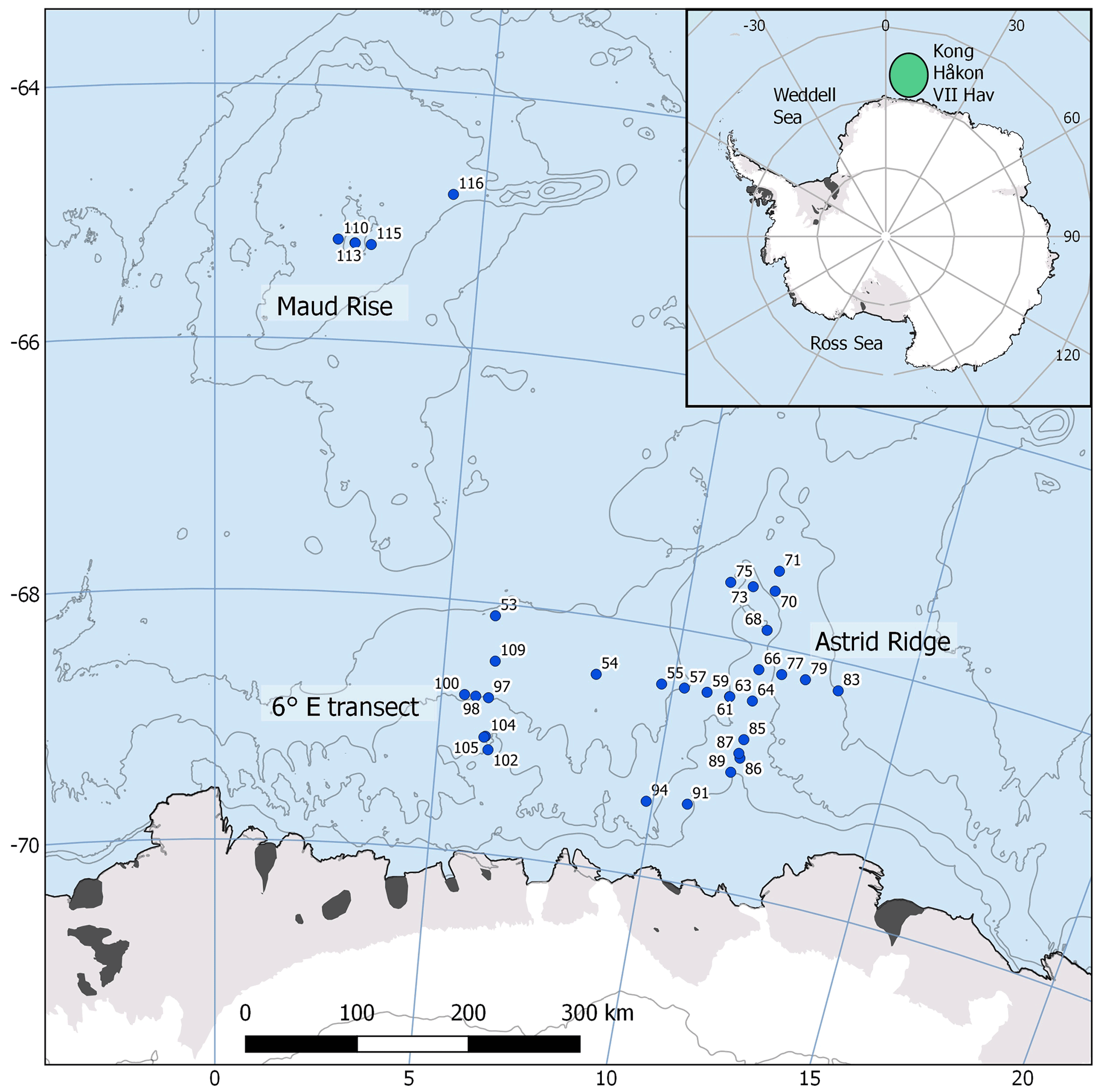
Figure 1 Map of the study area. The CTD stations with water sampling are marked with blue circles. The sampling area is marked with a green ellipse in the inset. The contour interval is 1000 m. Map created with the help of Quantarctica (Norwegian Polar Institute, 2018).

Selected environmental variables are presented in Kauko et al. (2021). In short, macronutrients (silicic acid, nitrate, and phosphate) were above limiting concentrations (33.0–93.8, 20.7–32.9, and 1.4–2.3 µM, respectively). Mixed layer depth (MLD) was on average 36 (± 13) m. Krill swarms occurred especially in the northern part of the 6^∘ E transect and to a lesser extent at Astrid Ridge, while mesozooplankton were most abundant at Maud Rise. Carbonate chemistry in the region is presented in Ogundare et al. (2021).

2.2 Water sampling and laboratory analyses

Water samples were collected from multiple depths in the upper 100 m at a total of 37 stations (station numbers starting with 53) between 12 and 31 March in connection with CTD (conductivity–temperature–depth) casts with a 24-bottle or 12-bottle SBE 32 carousel water sampler.

Samples for phytoplankton microscopy analyses (190 mL) were collected from three different depths (typically 10, 25 or 40, and 75 m), filled into 200 mL brown glass bottles and fixed with glutaraldehyde and 20 % hexamethylenetetramine-buffered formalin at final concentrations of 0.1 % and 1 %, respectively, and thereafter stored cool and dark. For analysis, 10–50 mL subsamples were settled in Utermöhl sedimentation chambers (HYDRO-BIOS©, Kiel, Germany) for 48 h and counted with a Nikon Ti-U inverted light microscope using the Utermöhl method (Edler and Elbrächter, 2010). Protist cells were counted in fields of view located along transects crossing the bottom of the chamber. In each sample, at least 50 cells of the dominant species were counted (a 95 % confidence limit of ± 28 % according to Edler and Elbrächter, 2010).

Flow cytometry (FCM) samples (4.5 mL) for counting cells in small algal size classes (picoplankton and nanophytoplankton, 0.7 to 2 µm and 2 to 20 µm, respectively) were collected in cryovials from five to six different depths, fixed with glutaraldehyde (0.5 % final concentration) and stored at −80 ^∘C until analyses at the University of Bergen. In the laboratory, samples were thawed, mixed gently and analyzed in an Attune^™ NxT Acoustic Focusing Cytometer (Invitrogen^™, Thermo Fisher Scientific Inc. USA) equipped with a 50 mW 488 nm (blue) laser. Quantification and discrimination of the different phytoplankton size classes was done with the help of bi-parametric plots based on side scatter and red fluorescence.

Samples for algal pigment analysis (usually 1 L) were collected from three different depths (typically 10, 25 or 40, and 75 m), filtered on 0.7 µm GF/F filters (GE Healthcare, Little Chalfont, UK) with a gentle vacuum pressure (approximately −30 kPa) and immediately stored in the dark at −80 ^∘C. Pigments were measured and quantified with a Waters Alliance 2695 HPLC Separation Module connected to a Waters photodiode array detector (2996). HPLC-grade solvents (Merck) and an Agilent Technologies Microsorb-MV3 C8 column (4.6 × 100 mm) were used for peak separation. The autosampler module was kept at 4 ^∘C during the measurements. In total, 100 µL of sample was injected with an auto addition function of the system between the sample and a 1 molar ammonium acetate solution in a ratio of $\mathrm{30}:\mathrm{20}:\mathrm{30}:\mathrm{20}$. Peak identification and quantification was obtained with the EMPOWER software. More details about the solvents and gradient can be found in Tran et al. (2013). An overview of the taxonomical distribution of pigments is given in Jeffrey et al. (2011), Higgins et al. (2011) and the data sheets of Roy et al. (2011).

2.3 Statistical analyses

Similarity and separation between the sampling areas in terms of the microscopy counts was evaluated with non-metric multidimensional scaling (NMDS) using the isoMDS function in the MASS package (Venables and Ripley, 2002) and the R software (R Core Team, 2017). Water samples down to 100 m depth with full taxonomical resolution were used for the analysis. Bray–Curtis dissimilarities (vegan package in R; Oksanen et al., 2017) were used for the scaling, and abundances were square-root transformed prior to that to reduce the effect of high and uneven abundances. The dissimilarities between the groups were further tested statistically with the anosim function from the vegan package. Test result values (R values) close to 0, as opposed to 1, indicate random grouping. For the test considering differences between the sampling areas, the assumptions of heterogeneity and similar sample size were not met; however, due to the lower range of dissimilarities occurring in the smaller-sized sample group Maud Rise (Fig. A1), the test tends to be overly conservative (Anderson and Walsh, 2013), and thus a significant result appears reliable.

To study the relationship of abiotic environmental variables and the community composition, a canonical correspondence analysis (CCA) was used from the vegan package. The included environmental variables were silicate and nitrate (Chierici and Fransson, 2020; Kauko et al., 2021), MLD, temperature and salinity (Kauko et al., 2021; Hattermann and de Steur, 2022). Phosphate correlated highly (0.90) with nitrate and was therefore not included; nitrate thus can be considered representative of both macronutrients. Missing environmental data were filled with the mean of that variable, and all environmental data were standardized by subtracting the mean of the data and dividing by the standard deviation. Phytoplankton species count data were mainly grouped into upper-level categories (corresponding to the main geographical features observed in the data and discussed in this paper) and included the following taxa: flagellates, dinoflagellates, pennate diatoms, centric diatoms and Chaetoceros dichaeta. These data were then square-root transformed. Originally, the analysis was conducted with full taxonomical resolution, but in this configuration only a small portion of the variance (11 %) was explained (figures not shown). The orientation of the figure was, however, largely similar.

Diversity in the phytoplankton community was investigated with Shannon's diversity index (H; function diversity in the vegan package) and species richness (number of species, genera and size groups of unidentified taxa). Differences between the areas and sampling depths were tested with one-way analysis of variance (ANOVA; function aov in R). The assumptions of homoscedasticity were met in the models.

2.4 CHEMTAX analysis

Phytoplankton community composition was further investigated by applying a factor analysis program called CHEMTAX (Mackey et al., 1996), which allows us to calculate the abundance of the various algal groups based on the measured marker pigments. As we had a large number of samples and no experimental or field information on local pigment ratios, the original approach (Mackey et al., 1996) was concluded to be more suitable than the Bayesian approach (Van den Meersche et al., 2008), according to Higgins et al. (2011). The CHEMTAX software package was obtained from Wright (2008).

The initial ratio matrix was based on the literature. Pigment-to-Chl a ratios for prasinophytes, chlorophytes, cryptophytes, two pigment types of diatoms and peridinin-containing dinoflagellates were taken from the table in Wright et al. (2010), a study that was conducted close to our study area (between 30 and 80^∘ E and south of 62^∘ S), with the following modifications. Chl c₁ was changed to Chl c₁₊₂ (which is the resolution of our chromatographic results), with values taken from the CHEMTAX material (geometric means of reported ratios from the literature collected in Higgins et al., 2011). The values for 19^′-butanoyloxyfucoxanthin (but-fuco) and ratios for haptophyte pigment type 6 and for dinoflagellate pigment type 2 (microscopy revealed the dominance of Gymnodinium spp.) were taken from Table 6.1 in Higgins et al. (2011). Zeaxanthin was observed in only one sample and was omitted from the analysis. Diadinoxanthin, diatoxanthin and β,β-carotene were excluded because they are not very group-specific. Neoxanthin, prasinoxanthin and violaxanthin were not observed in the samples and were removed from the ratio matrix.

Haptophytes belong to several (eight) different pigment types (Zapata et al., 2004) and in addition change their marker pigment content according to environmental conditions such as iron availability (van Leeuwe and Stefels, 1998; Wright et al., 2010). Therefore, all haptophyte pigment types were initially tested with CHEMTAX runs on all samples (20 randomized ratio matrices, using the pigment ratios from the CHEMTAX material mentioned above as initial ratios). Pigment type 8 is typical in the Southern Ocean including the species P. antarctica, whereas coccolithophores belong to pigment type 6. Out of the eight different pigment types tested, including pigment types 6, 7 or 8 resulted in the lowest root mean square errors (RMSEs; below 0.2). Pigment type 7 includes, e.g., the genus Chrysochromulina, which is not typical in the Southern Ocean. Including both haptophyte types 6 and 8 (in different ratio range categories according to the CHEMTAX instructions) also resulted in a low RMSE, and for the categories with a high ratio range for haptophyte type 6 the error was lowest and similar to when including only haptophyte type 6 (<0.15). However, coccolithophores should not be abundant this far south (Balch et al., 2016; Saavedra-Pellitero et al., 2014; Trull et al., 2018) and were not observed in the microscopy samples. Other prymnesiophytes were not abundant either – only P. antarctica was observed in only three CTD samples. This taxon has a characteristic appearance and, if present in large quantities, would likely have been identified, whereas the majority of flagellates in the microscopy samples were classified as unidentified flagellates in the 3 to 7 µm size range. Therefore, to simplify the analysis (e.g., to avoid having too many algal groups compared to pigments, Mackey et al., 1996) and to account for the unidentified status of this group, we have included only one haptophyte group in the final runs with the best-performing, i.e., type-6, pigment ratios, and called this “Haptophyte-6-like”. Silicoflagellates and chrysophytes, which were observed at low abundances in microscopy samples (maximum abundances of 3900 and 18 200 cells L⁻¹, respectively), will also be included in the haptophyte pigment group, as they contain similar pigments, e.g., Chl c, fucoxanthin and its derivatives (Jeffrey et al., 2011).

In the preliminary analysis, it was also tested to separate the samples into different clusters. With all the samples combined, including only the surface samples down to 10 m or successively adding depth ranges one at a time did not improve the result in terms of the RMSE compared to including all the depths. Separating Maud Rise from the rest reduced the error when different area clusters were tested with all the samples. Trials indicated that dividing the Maud Rise samples into depth clusters may bring further improvements, but as the number of samples was relatively small (in total, 12 CTD samples from Maud Rise), they were kept as one cluster. Astrid Ridge had a larger number of samples (55 in total) and was divided into two clusters (above and below including 40 m; the average MLD was 34 m; Kauko et al., 2021) and separated from the rest, which reduced the error. For the 6^∘ E transect, separating the surface samples did not reduce the error.

In total, there were 98 samples from the CTD casts. In the clusters Maud Rise, Astrid Ridge surface, Astrid Ridge deep and other stations (stations 53 and 54 and the 6^∘ E transect) there were 12, 26, 29 and 31 samples, respectively. After the first 60 runs for each of the clusters (using 60 randomized pigment ratio matrices based on the initial ratio matrix), the average output ratio matrix of the 6 best runs was used as the initial ratio matrix for the next 60 runs. The reported results are the averaged output from the six best runs of this second step.

3 Results

3.1 Microscopy

The microscopy data are shown here as averages per sampling area and for the most important taxa separately, whereas others are summed together into higher-level categories such as “Pennate diatoms (other)”. All taxa are listed in Table B1 together with median abundances and occurrence in the different sampling areas, and variance in data used for the averages (i.e., data from all samples) is shown in Figs. A2 and A3. The complete dataset can be found in Kauko et al. (2022).

Two of the sampling locations stood out in terms of higher diatom abundances. Average diatom abundances at station 53 and Maud Rise reached 5.2 × 10⁵ and 7.5 × 10⁵ cells L⁻¹, respectively (Fig. 2a), and Chl a data showed that these locations had the highest biomass in the area (Fig. 3; Kauko et al., 2021). Most of the sampling areas were dominated by diatoms in terms of average abundances, most notably for the area represented by station 53 and Maud Rise (74 % and 89 %, respectively), whereas at station 54 or Astrid Ridge the dominance was less pronounced (62 % and 56 %), and the area along the 6^∘ E transect was slightly dominated by flagellates (45 % flagellates compared to 36 % diatoms). At Maud Rise flagellates and dinoflagellates occurred in similar abundances, whereas in the other areas, flagellates were more abundant than dinoflagellates, most notably so along the 6^∘ E transect. Ciliates and cyanobacteria (unidentified filamentous blue-green algae; cf. Anabaena sp.; see the photo in Fig. A4) were also observed at very low abundances, especially the latter mainly at Astrid Ridge and along the 6^∘ E transect. FCM biplots (Fig. A5) using orange fluorescence indicated the presence of cyanobacteria in the corresponding samples; however, abundances were low, and the filamentous nature of the cyanobacteria complicates interpretations for this method.

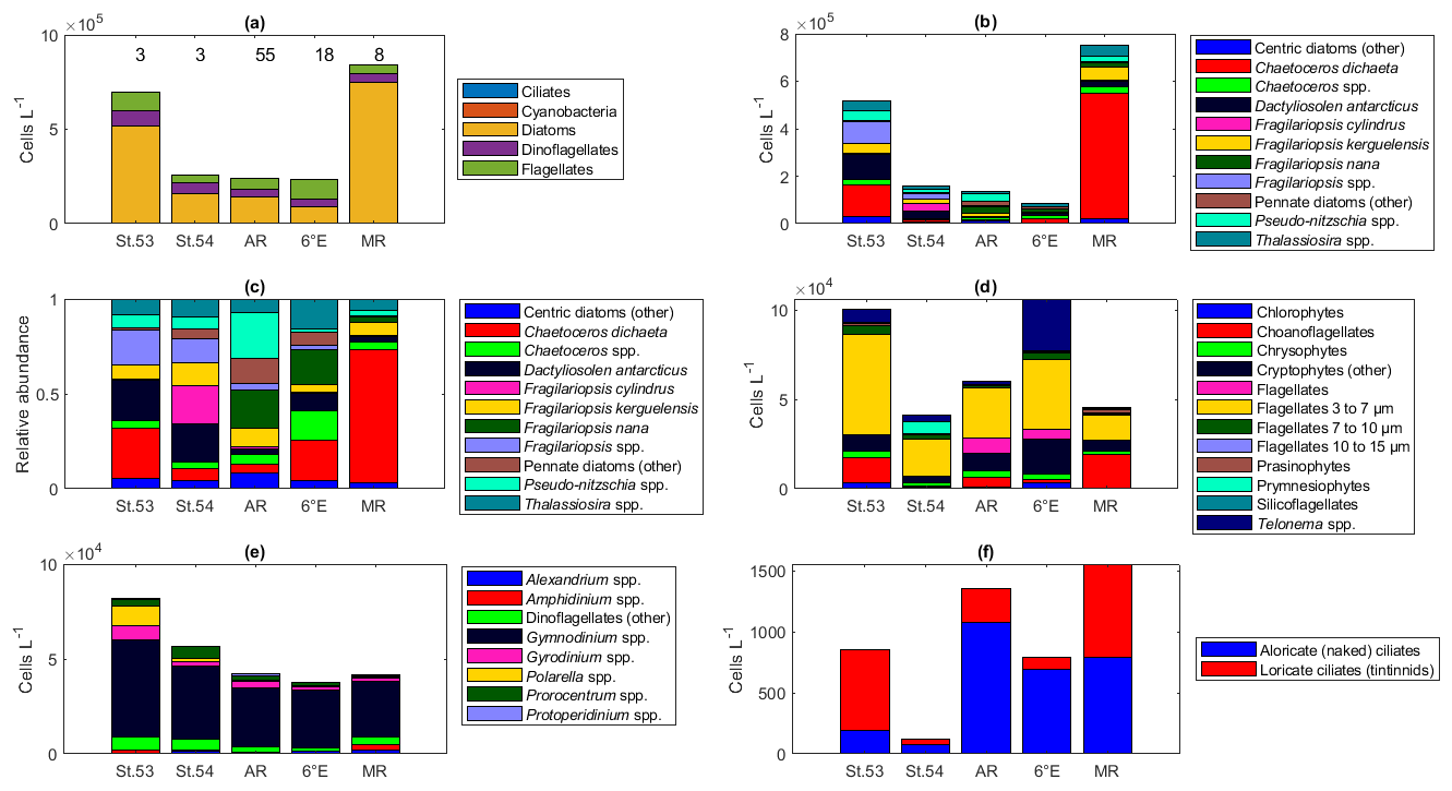
Figure 2 Abundance of different protist groups and species for the (a) main taxa, (b) diatoms, (c) relative abundance of diatoms, (d) flagellates, (e) dinoflagellates, and (f) ciliates. In panel (a), the number of samples used for the average abundances is shown at the top of the figure (the numbers apply to all the figures). In panels (c) and (d), the genera Fragilariopsis and Pseudo-nitzschia belong to pennate diatoms, and thus pennate diatoms are shown with colors pink/yellow to cyan. St.53: station 53, St.54: station 54, AR: Astrid Ridge, 6E: 6^∘ E transect, MR: Maud Rise.

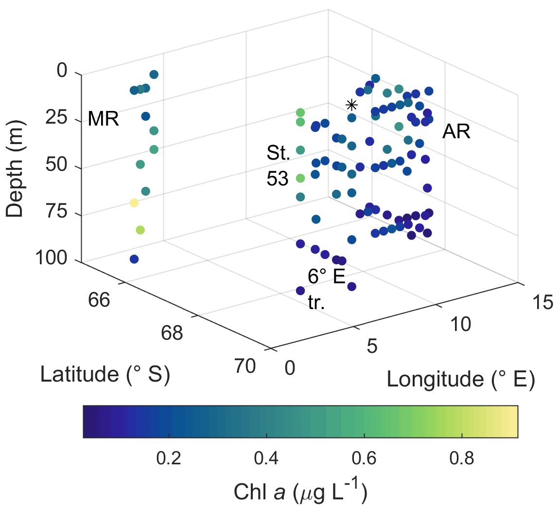
Figure 3 Horizontal and vertical distribution of phytoplankton biomass expressed as Chl a concentration. MR: Maud Rise, St. 53: station 53, AR: Astrid Ridge, 6^∘ E tr.: 6^∘ E transect. Station 54 is marked with a black asterisk.

The dominance patterns were similar when abundances were averaged per depth interval (Fig. A6). In terms of abundances, phytoplankton were concentrated in the upper 40 m at station 53 and Astrid Ridge, whereas along the 6^∘ E transect the generally low abundances were more evenly distributed with depth, and at Maud Rise the bloom extended deeper with relatively high cell numbers (4 × 10⁵ cells L⁻¹) until 75 m.

Among the diatoms, C. dichaeta clearly dominated station 53 and Maud Rise communities down to 40 and 50 m, respectively (Figs. 2b–c, 4 and A7). Chaetoceros dichaeta formed 59 % of the diatom community at 10 m and 40 % at 40 m at station 53; i.e., it was the most abundant species at these depths. At Maud Rise, besides the surface samples, C. dichaeta dominated the diatom community at 100 m depth (at station 110; Fig. A8). This species was also an important component of the 6^∘ E transect diatom community, although at much lower abundances. In these other sampling areas (the 6^∘ E transect, station 54 and Astrid Ridge), the abundances of various diatom species were more evenly distributed. Other important taxa were Fragilariopsis spp., F. nana, F. kerguelensis, F. cylindrus, Dactyliosolen antarcticus, Chaetoceros spp. and Pseudo-nitzschia spp. At Astrid Ridge and station 54, pennate diatoms (particularly Fragilariopsis spp. and Pseudo-nitzschia spp.) were more abundant than centric diatoms, with shares of 72 % and 56 %, respectively. In other areas pennate diatoms contributed 14 % to 34 %. Overall, there were 89 diatom taxa (at the genus or species level) identified during this research campaign.

Maximum average abundances of flagellates were observed at station 53 and along the 6^∘ E transect, with 1.0 × 10⁵ and 1.1 × 10⁵ cells L⁻¹, respectively (Fig. 2d). Among the flagellates, the majority were categorized as unidentified flagellates in the size range 3 to 7 µm. Cryptophytes and especially the genus Telonema were also a notable component of the flagellate community in many of the areas (in Fig. 2d, cryptophytes and the genus Telonema are presented separately). Choanoflagellates (heterotrophic flagellates) were observed at relatively high numbers at station 53 and Maud Rise. Phaeocystis antarctica (the only prymnesiophyte species identified) was found at station 54, mainly at 40 m, but it was not an abundant species during the cruise, which was also confirmed by microscope analysis of live material from net samples taken from the upper 20 m at every CTD station during the cruise. Chlorophytes, chrysophytes, prasinophytes, and silicoflagellates were also observed in minor numbers. The depth distribution of flagellates (figures not shown) was largely similar to the composition of the whole-area averages.

Dinoflagellates belonged mainly to different, unidentified species of the genus Gymnodinium in all areas (Fig. 2e) and at all depths (figures not shown). Additionally, the genera Prorocentrum, Gyrodinium, Alexandrium, Amphidinium, Polarella and Protoperidinium were also present. The maximum average dinoflagellate abundance was observed at station 53 (8.2 × 10⁴ cells L⁻¹).

Ciliates were present in lower numbers (the maximum average abundance was 1500 cells L⁻¹ at Maud Rise; Fig. 2f) but with several species (16 species or higher-level taxa; Table B1). The most notable species were Salpingella costata, Strombidium spp., and Lohmanniella oviformis as well as Uronema marinum at station 53 and Mesodinium rubrum at station 54. At Astrid Ridge and along the 6^∘ E transect, aloricate (naked) ciliates dominated in abundance (at station 54 the dominance was less pronounced), whereas at Maud Rise the abundances were even and at station 53 loricate ciliates (tintinnids) dominated (Fig. 2f).

Shannon's diversity index varied between 0.9 and 3.4 and the species richness between 11 and 65 species/taxa. The biodiversity between the areas was relatively similar, but the most notable geographical patterns were that most depths at Maud Rise had a low diversity index and that species richness in the other sampling areas was lower at depth than in the upper part of the water column (Fig. 5a and b). This was also visible in the statistical analysis of differences between groups: regarding the diversity index, the differences between areas were highly significant (p value < 0.001), but not between depth categories (p value 0.32; the same depth categories were used as in Fig. 4). A post hoc Tukey test confirmed that Maud Rise differed from all the other areas (p value < 0.02 for all comparisons). For species richness the inverse was found: differences between depth categories were significant (p value < 0.001) and not between the areas (0.69). A post hoc Tukey test showed that the surface depth categories (10, 25 and 40 m) differed from the deeper categories (50 and 75 m; p value for all comparisons <0.02, except for between 50 and 25 m, where the p value was 0.06); that is, species richness was significantly lower at depth (50 m and deeper). The means for the different areas were 2.7, 3.0, 2.7, 2.6 and 1.9 for the diversity index and 49, 47, 44, 45 and 49 for species richness for station 53, station 54, Astrid Ridge, the 6^∘ E transect and Maud Rise, respectively. The mean diversity index was thus significantly lower at Maud Rise. The diversity index did not have a clear correlation with biomass, but species richness increased with increasing biomass up to maximum values of around 55–65 (Fig. 5c and d).

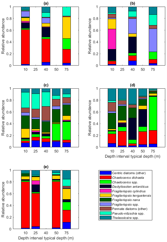
Figure 4 Diatom relative abundance in the different sampling areas averaged per depth interval for (a) station 53, (b) station 54, (c) Astrid Ridge, (d) the 6^∘ E transect and (e) Maud Rise. Depth intervals (with typical sampling depth in brackets): 5–10 (10), 25–35 (25), 35–45 (40), 50–60, and 65–85 (75) m.

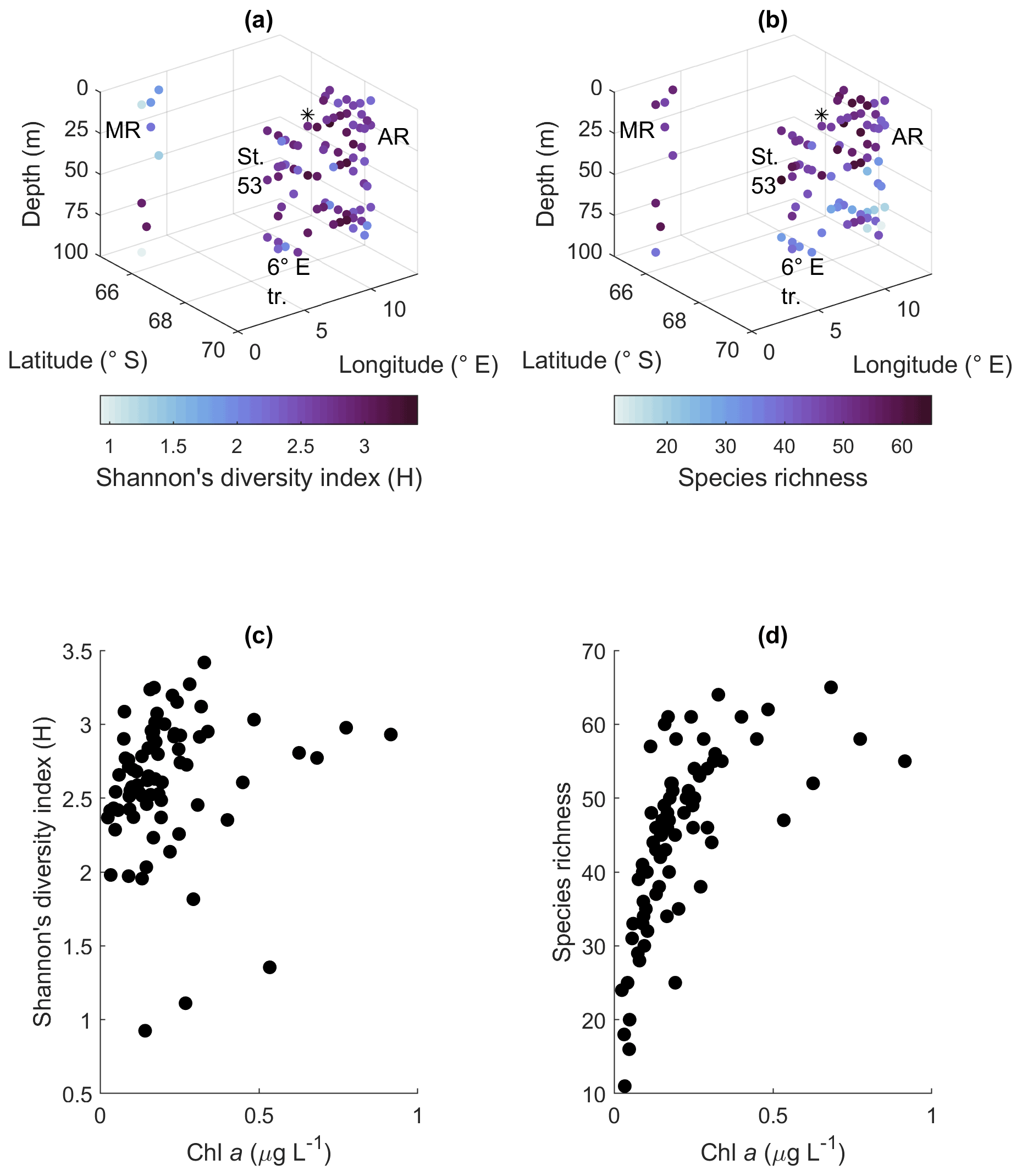
Figure 5 Biodiversity according to the microscopy samples. (a) Shannon's diversity index, (b) species richness, (c) relationship between algal biomass (expressed in Chl-a concentration) and Shannon's diversity index and (d) algal biomass and species richness. MR: Maud Rise, St. 53: station 53, AR: Astrid Ridge, 6^∘ E tr.: 6^∘ E transect. Station 54 is marked with a black asterisk.

3.2 Statistical analysis of the sampling areas

Clustering (NMDS) of the species abundance results from the microscopy analysis showed that the communities in the different sampling areas (marked with different symbols in Fig. 6) did not separate into distinct clusters, but they appear located on different sides of the cluster, with stations 53 and 54 and Maud Rise samples on the one side and Astrid Ridge and 6^∘ E transect samples predominantly on the other side. In addition to the diatom blooms in the first two mentioned areas, this could also reflect a coastal-to-offshore pattern. However, the low R value of 0.15 from the anosim test (significance 0.017) indicated overall a high similarity between the areas.

In addition, a separation along the sampling depth gradient (color scale in Fig. 6) is clearly visible, with the surface samples (typically sampled at 25 m depth) and the deep samples (typically sampled at 75 m depth) located on different sides of the cluster. The anosim test indicated a somewhat higher degree of differentiation between the depth clusters (R value 0.27, significance 0.001) than between the sampling areas. In addition, when the NMDS analysis is performed on presence–absence data (Fig. A9), it is difficult to separate the areas, but the sampling depth pattern is still visible, though the samples are very condensed on the plot. Other categorizations included in the analysis, such as bottom depth, latitude or separation of Astrid Ridge into different areas (northern, southern, western and eastern parts of the ridge), did not yield such clear patterns (figures not shown).

Similarly, in the CCA analysis (Fig. 7), the sampling areas are distributed along the first axis (explaining 38.8 % of the variance) although not completely separated. The environmental variables that best explain the first axis are silicate and MLD. Maud Rise and station 53 (in addition to some stations at the 6^∘ E transect) are thus associated with deeper MLD and higher silicic acid concentrations as well as higher salinity and temperature. Nitrate best explains the second axis, although this axis only explains a small portion of the variance (4.2 %). The different stations, especially at Astrid Ridge, and to a lesser extent at the 6^∘ E transect, are spread along the second axis.

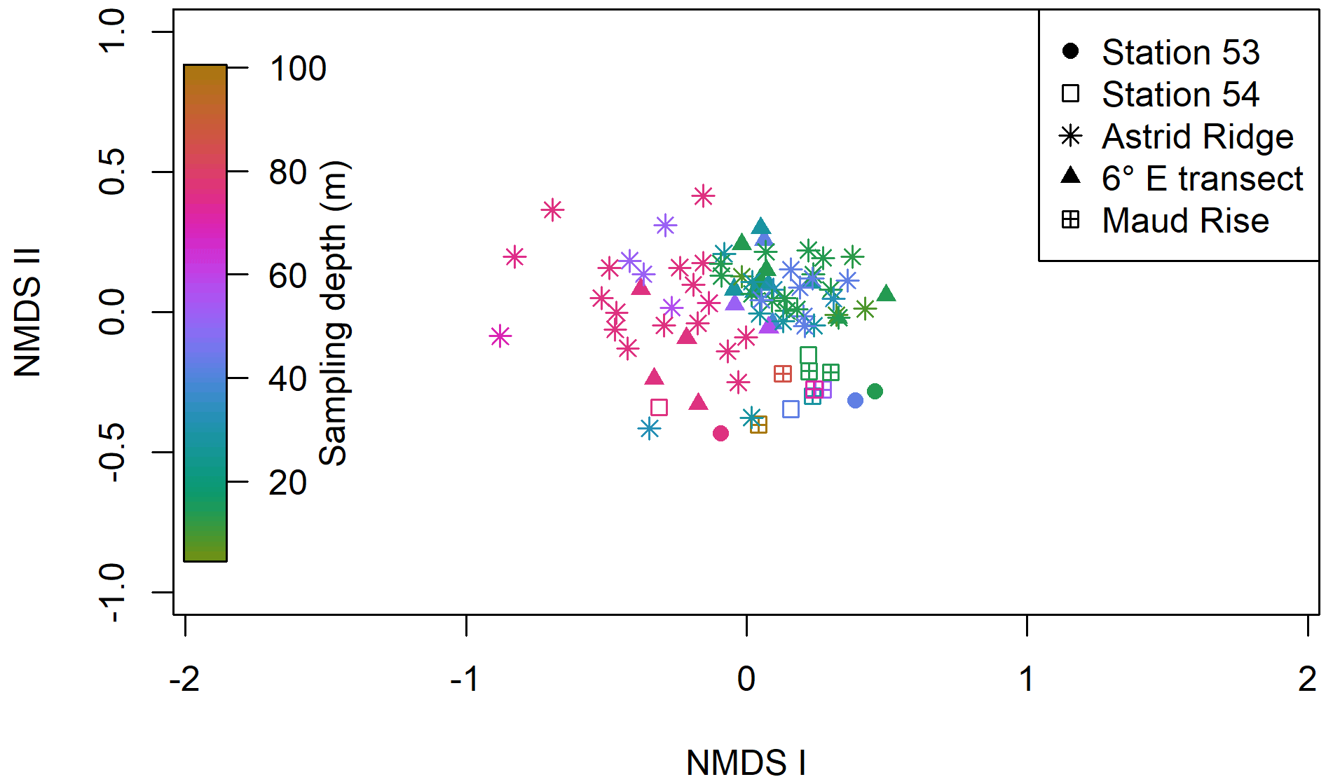
Figure 6 Results of the NMDS clustering of the microscopy count samples. The color shows the sampling depth, and the different sampling areas are shown with different symbols; see the legend. The stress value of the plot is 22 %.

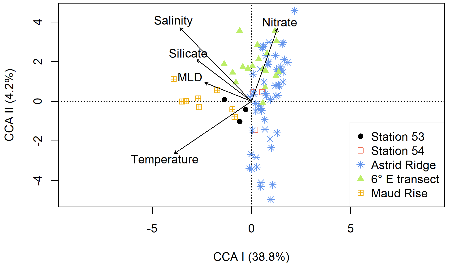
Figure 7 Results of the CCA analysis using microscopy count data at a coarse resolution (see “Methods”) and key chemical and physical oceanographic variables. Samples from the different sampling areas are differentiated by color and symbol; see the legend.

3.3 Flow cytometry

Smaller nanophytoplankton (Nanophytoplankton 1; Fig. A5) showed the highest abundances along the 6^∘ E transect, with abundances up to 4.7 × 10⁶ cells L⁻¹ (Fig. 8a), and the lowest at Maud Rise. By contrast, larger nanophytoplankton (Nanophytoplankton 2) were associated with Maud Rise and station 53 (up to 4.2 × 10⁶ cells L⁻¹; Fig. 8b). Maud Rise had high abundances also at depth, in contrast to station 53. Some larger cells (Nanophytoplankton 2) were also observed on top of Astrid Ridge (stations 66, 68 and 73), near the surface.

Picophytoplankton abundance was lower than for nanophytoplankton (up to 0.7 × 10⁶ cells L⁻¹; Fig. 8c), but a few stations on the western side of Astrid Ridge (57, 59, 61) showed a distinct picophytoplankton population in the FCM biplots (Fig. A5).

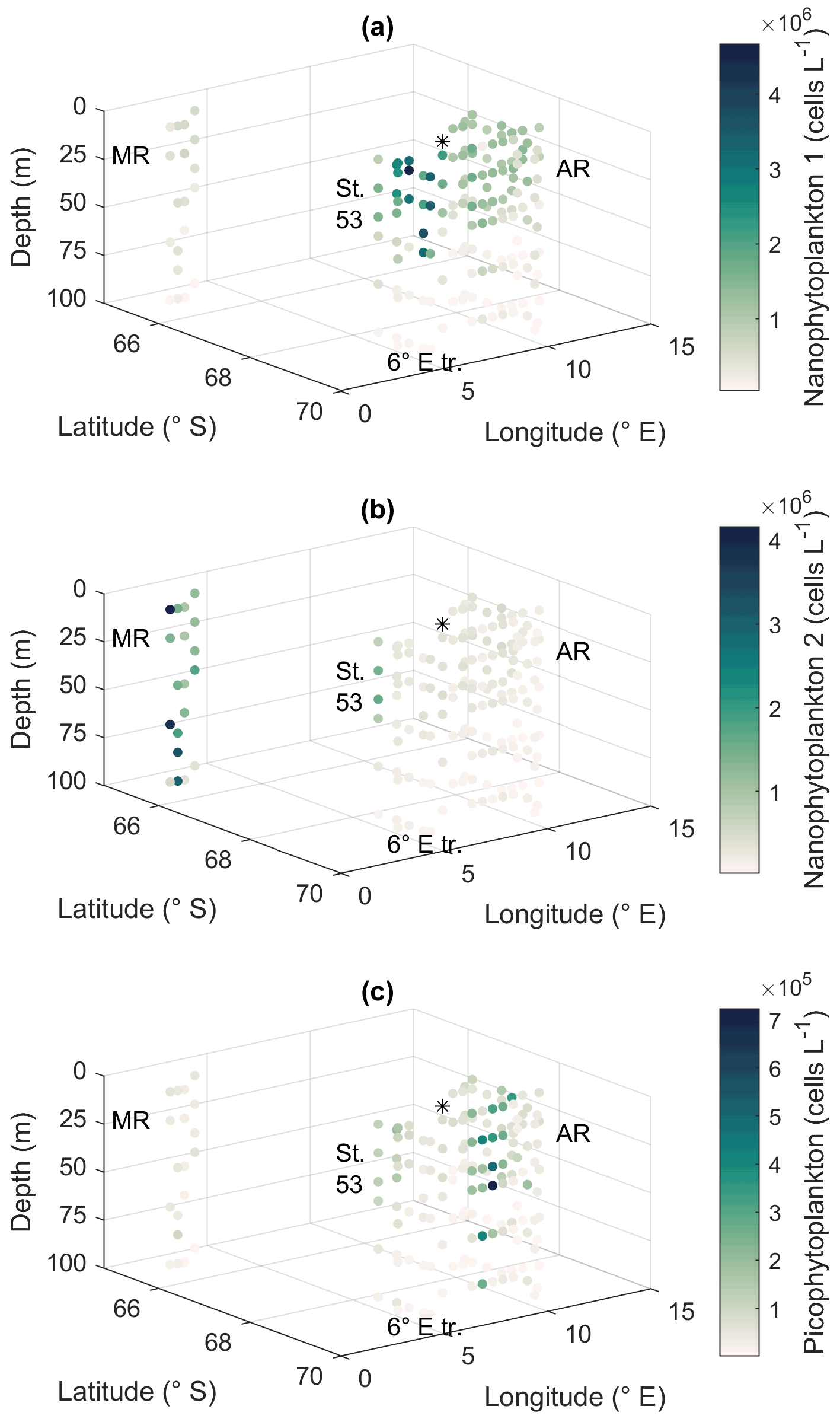
Figure 8 Flow cytometry results. Cell abundances of two groups of nanophytoplankton (a, b) and picophytoplankton (c). MR: Maud Rise, St. 53: station 53, AR: Astrid Ridge, 6^∘ E tr.: 6^∘ E transect. Station 54 is marked with a black asterisk.

3.4 Marker pigments

Pigment-to-Chl a ratios are presented in Figs. 9 and A10 and reported here, whereas the pigment concentrations are shown in Figs. A11 and A12. Pigment-to-Chl a ratios indicate the relative community composition better than the absolute concentrations. Chl a concentration ranged between 0.02 and 0.92 µg L⁻¹ (Fig. 3). The diatom blooms at Maud Rise and station 53 and the importance of flagellates at the 6^∘ E transect were also visible in the pigment data.

Ratios of fucoxanthin, a typical pigment in diatoms, to Chl a were very high at Maud Rise and station 53, up to 0.93 (Fig. 9a). The ratios were the lowest at the 6^∘ E transect, with a minimum of 0.12. At Astrid Ridge the ratios were in between these values, at around 0.5. The ratios of Chl c₁₊₂ to Chl a were also the highest at Maud Rise and station 53, up to 0.70, and seemed thus to be primarily associated with fucoxanthin and diatoms (Fig. 9b). However, other Chl-c₁₊₂-containing groups were also likely present, as the ratios at the flagellate-dominated 6^∘ E transect did not differ from the other areas as much as for fucoxanthin.

Chl c₃ showed the highest pigment-to-Chl a ratio values at the 6^∘ E transect and at depth at Astrid Ridge, up to 0.55 (Fig. 9c). It was also found at Maud Rise at all depths, in the surface waters at station 53 and station 54, and at Astrid Ridge mainly in the middle of the ridge, from the surface to the mid-depths. This pigment thus further indicates that flagellates were an important part of the 6^∘ E transect community, as it is a major pigment, e.g., in haptophytes. In addition, 19^′-hexanoyloxyfucoxanthin (hex-fuco), another important pigment in haptophytes, showed clearly its highest pigment-to-Chl a ratio values at the 6^∘ E transect, up to 1.01, and the lowest at Maud Rise (Fig. 9d). Another fucoxanthin derivative, but-fuco, which is mainly found in pelagophytes, silicoflagellates and some haptophytes, showed the highest pigment-to-Chl a ratio values at depth at the 6^∘ E transect and Astrid Ridge, but values were low (Fig. 9e).

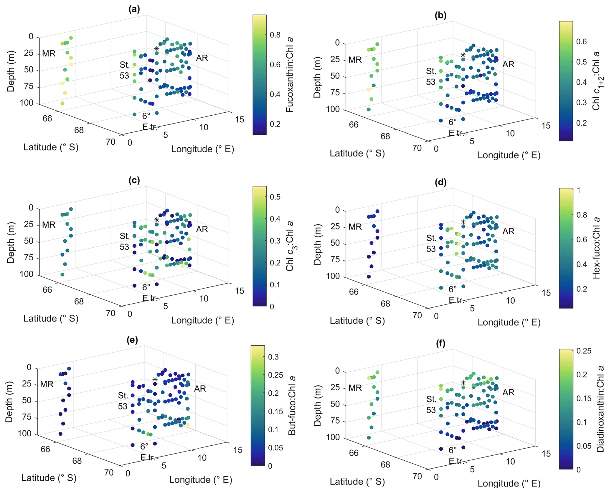
Figure 9 Ratios of algal pigments to Chl a for (a) fucoxanthin, (b) Chl c₁₊₂, (c) Chl c₃, (d) hex-fuco, (e) but-fuco and (f) diadinoxanthin. MR: Maud Rise, St. 53: station 53, AR: Astrid Ridge, 6^∘ E tr.: 6^∘ E transect. Station 54 is marked with a black asterisk.

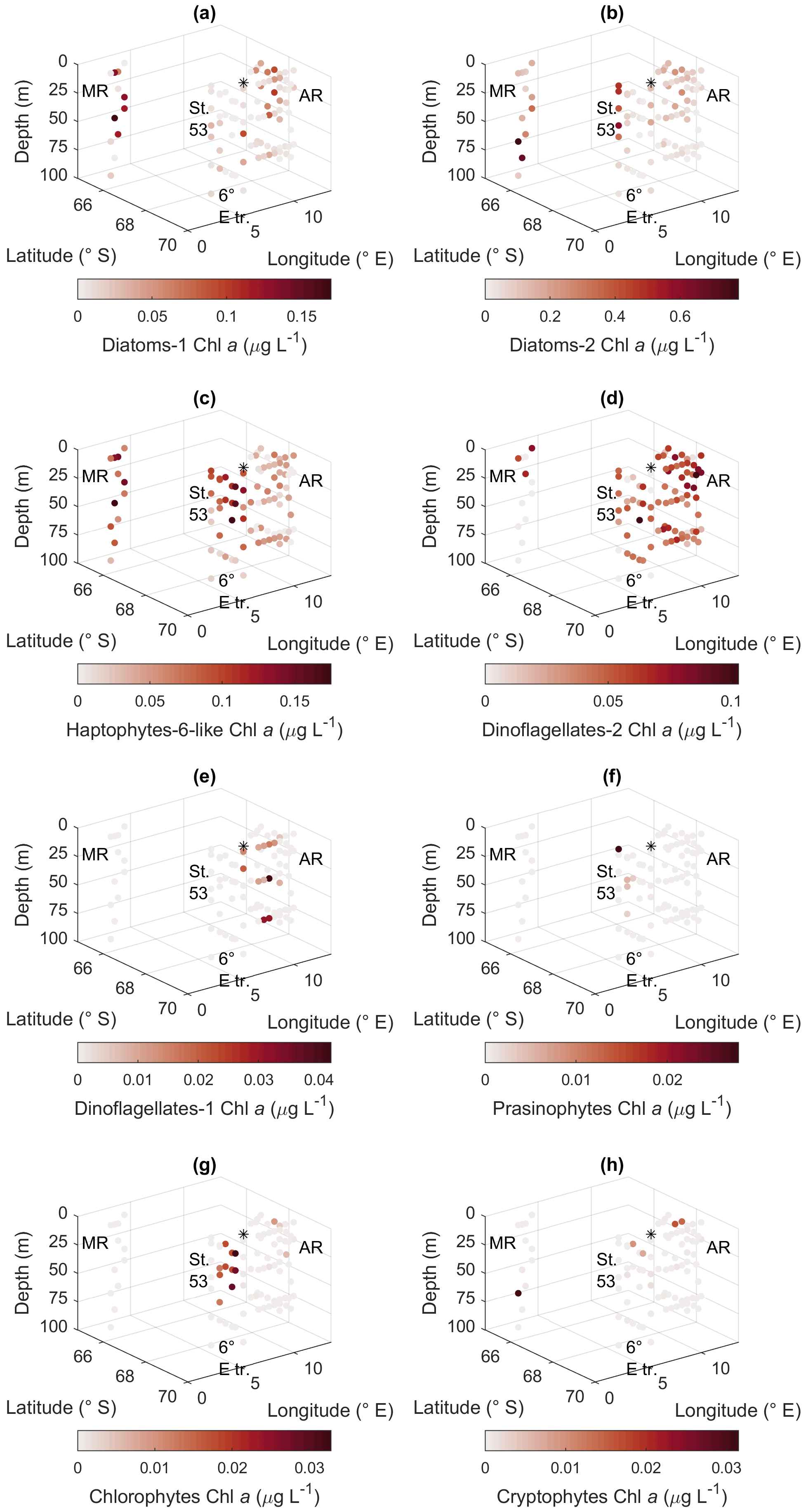
Figure 10 CHEMTAX results for the different algal groups. (a) Diatom type 1, (b) diatom type 2, (c) haptophyte type 6-like, (d) dinoflagellate type 1, (e) dinoflagellate type 2, (f) prasinophytes, (g) chlorophytes, and (h) cryptophytes. MR: Maud Rise, St. 53: station 53, AR: Astrid Ridge, 6^∘ E tr.: 6^∘ E transect. Station 54 is marked with a black asterisk.

Diadinoxanthin, a carotenoid participating in the photoprotective xanthophyll cycle, occurred in the highest pigment-to-Chl a ratios close to the surface in all the areas (up to 0.25), but at Maud Rise relatively high ratios were observed throughout the sampling depths (Fig. 9f). Diatoxanthin, its counterpart in the xanthophyll cycle, was observed in five samples at a much lower concentration (5 %–16 % of diadinoxanthin). It should be noted that although the samples were processed as quickly as possible, they were part of a larger sampling effort, and conversion from diatoxanthin to diadinoxanthin may have happened during the storage under dark conditions.

Peridinin (a major pigment in one of the dinoflagellate pigment classes), alloxanthin (a major pigment in cryptophytes), lutein (Chl-b lineage, e.g., chlorophytes and prasinophytes) and Chl b were observed in minor amounts in certain areas (Fig. A10): peridinin on the western side of Astrid Ridge (pigment-to-Chl a ratio up to 0.15), alloxanthin at the surface at a few stations of the 6^∘ E transect and Astrid Ridge (up to 0.01), and lutein and Chl b at the 6^∘ E transect (up to 0.04 and 0.06, respectively). β,β-carotene is not very taxon-specific and did not show clear geographical patterns (pigment-to-Chl a ratio up to 0.05; Fig. A13). Zeaxanthin was only observed in one sample, on the surface (5 m) at station 70 at Astrid Ridge, in a low concentration (the ratio to Chl a was 0.02). All pigment data can be found in Moreau et al. (2020).

3.5 CHEMTAX analysis

The CHEMTAX analysis is a way to distinguish and quantify the contribution of various phytoplankton groups based on the measured marker pigment concentrations. In total, eight phytoplankton groups were included in the analysis based on prior knowledge from the microscopy results and the literature. Clear geographical patterns were observed in the distribution of the groups, in line with the other phytoplankton data sources. Diatom pigment type 2 (diatoms containing Chl c₃) had the highest biomass, followed by diatom type 1 and the haptophyte-like group (Fig. 10). Diatom type 1 ranged up to 0.17 µg Chl a L⁻¹ and had the highest values in the upper water column at Astrid Ridge and Maud Rise. Diatom type 2 was most prominent at station 53 and at depth at Maud Rise, with a maximum value of 0.78 µg Chl a L⁻¹. Haptophyte-6-like had the highest values at Maud Rise and the upper water column at the 6^∘ E transect with a maximum value of 0.18 µg Chl a L⁻¹ but a clear presence also at Astrid Ridge. Of the dinoflagellate groups, type 2 had higher biomass and was present in all areas, though only at the surface at Maud Rise, with a maximum value of 0.10 µg Chl a L⁻¹. Occurrence of dinoflagellate type 1 (peridinin-containing dinoflagellates), prasinophytes, chlorophytes and cryptophytes in the CHEMTAX results (Fig. 10) followed closely the distribution of their respective marker pigments (Figs. A10 and A12) and was correspondingly scattered and scarce. A maximum value of 0.04 µg Chl a L⁻¹ was found for dinoflagellate type 1 and 0.03 µg Chl a L⁻¹ for the other three groups. From the Chl-b-containing groups, chlorophytes were more abundant than prasinophytes, with a clear presence along the 6^∘ E transect.

The final RMSE for the clusters Maud Rise, Astrid Ridge surface, Astrid Ridge deep and other stations (stations 53 and 54 and the 6^∘ transect) was 0.017, 0.064, 0.080 and 0.069, respectively (average RMSE of the six best runs). The final output ratio matrices for each of the clusters are presented in Table B2 for potential use as initial ratio matrices in future studies in the area. It is noteworthy that differentiating the data between the sampling areas, and in some cases along the depth gradient, improved the results.

4 Discussion

4.1 Community patterns at the regional scale

The early autumn phytoplankton community composition in the Kong Håkon VII Hav was dominated by diatoms and other algae from the Chl-c lineage, which is typical for the open Southern Ocean (e.g., Buck and Garrison, 1983; Davidson et al., 2010; Kang and Fryxell, 1993; van Leeuwe et al., 2015; Nöthig et al., 2009; Peeken, 1997; Smetacek et al., 2004; Wright et al., 2010). Although the communities in the different sampling areas were largely similar (Fig. 6), some differences in the relative abundance of the major taxa were observed between the sampling areas, which will be discussed in the sections below. Furthermore, also in relation to the main oceanographic variables, the different areas showed some separation in a CCA analysis (Fig. 7). In particular, Maud Rise and station 53 can be considered more oceanic, with, in general terms, higher temperatures and salinity and a deeper MLD. Silicic acid was present in lower concentrations in surface waters at Maud Rise (Kauko et al., 2021), likely due to drawdown by the phytoplankton bloom, but concentrations in the depth at both Maud Rise and station 53 were higher than at Astrid Ridge and the 6^∘ E transect and may help to sustain blooms of this type with the dominance of a heavily silicified species (see also Sect. 4.3).

When it comes to biodiversity, phytoplankton species richness was similar between the areas investigated. The Maud Rise bloom had lower diversity indices, which can be attributed to the dominance of C. dicheata during the bloom (Vallina et al., 2014) and hence likely does not reflect persistent lower diversity at Maud Rise compared to the other areas – both species richness and evenness in abundances between species are components of biodiversity. The diversity index and species richness sampling area averages in our study were clearly higher than cluster averages in a community composition study conducted at 30–80^∘ E in austral summer (Davidson et al., 2010), and the diversity indices were relatively high for the low biomass level compared to a global data compilation (Irigoien et al., 2004).

Our pigment composition was very similar (though with lower maximum concentrations) to a study by Gibberd et al. (2013) that was conducted mainly at the prime meridian and the Weddell Sea in January–February 1 decade earlier. Surprisingly, including haptophyte pigment type 6 (“type species” coccolithophore Gephyrocapsa huxleyi, formerly known as Emiliania huxleyi; Bendif et al., 2019) gave better results (lower error) in the preliminary CHEMTAX analysis than including pigment type 8 (e.g., Phaeocystis), and when including both pigment types, type 6 was clearly more prominent. However, coccolithophores are not abundant this far south in the Southern Ocean (Balch et al., 2016; Saavedra-Pellitero et al., 2014; Trull et al., 2018), which is confirmed by our microscopy analysis. A few stations in the flow cytometry data may have had low abundances of coccolithophores (not shown; based on high side scattering and red fluorescence), but neither of these data indicated a strong presence of this group throughout the study. Although blooms of P. antarctica are a prominent feature in the marginal ice zones of the Ross Sea (Arrigo et al., 1999) and the Weddell Gyre (Vernet et al., 2019), P. antarctica or other prymnesiophytes were not abundant in our microscopy samples. This is consistent with the observation that blooms of P. antarctica are generally rare in the land-remote ACC (Smetacek et al., 2004) and is further supported by the low contribution of P. antarctica to bloom biomass in iron fertilization experiments conducted in the iron-limited Southern Ocean (Boyd et al., 2007). Even the LOHAFEX iron fertilization experiment conducted in low-silicate waters with a significant seed population of small initial P. antarctica colonies did not result in a bloom of this species, presumably because of strong top-down control by copepod grazers (Schulz et al., 2018). Furthermore, blooms of P. antarctica seem to coincide with the sea ice retreat and ice edge (Davidson et al., 2010; Kang and Fryxell, 1993; Vernet et al., 2019). Our sampling effort was conducted later in the season (i.e., early autumn, at the onset of sea ice formation) and could therefore partly explain why the species was observed at low abundances. A subsequent cruise along the 6^∘ E transect area earlier in the season (in December 2020–January 2021) observed higher abundances of P. antarctica (Sebastien Moreau et al., unpublished data).

Given the low contribution of both coccolithophores and P. antarctica, we have called the pigment group we included in the final CHEMTAX analysis “Haptophyte-6-like” to acknowledge that the exact identity of this group is unclear and can contain other types of algae that have similar pigment ratios to the haptophyte 6 group. The microscopy analysis indicated that the majority of the flagellates were different types of unidentified flagellates in the size group 3 to 7 µm (note however that this group may and likely did also contain heterotrophic flagellates). It should also be noted that, due to the similarities in pigments and pigment ratios, this pigment group will also contain silicoflagellates and chrysophytes. The former have a characteristic appearance and should have been reliably identified in the microscopy samples, and thus their share in the pigment group should be as low as in the microscopy abundances. Unidentified chrysophytes by contrast could have formed a considerable share of this pigment group. Chrysophytes were regularly observed in our microscopy samples, albeit not in high abundance. Unfortunately, pigment-to-Chl a ratio data are lacking for this group in the Southern Ocean. It is also important to note that CHEMTAX is a statistical approach whose success depends on the correct allocation of algal groups and pigment ratios. For unambiguous distinction between haptophytes and dinoflagellates-2, additional pigments, such as other fucoxanthin derivatives, are needed (see, e.g., Mendes et al., 2018). With the lack of those, concurrent microscopy analysis is essential for confirming the algal groups present.

Finally, picophytoplankton was not abundant in the area compared to nanophytoplankton – maximum picophytoplankton abundance was 15 % of maximum nanophytoplankton abundance, and only at certain stations was a distinct picophytoplankton occurrence observed in the FCM biplots. The absence of coccoid cyanobacteria in the area contributes to low picophytoplankton abundance. Likewise, Rembauville et al. (2017) observed a low picophytoplankton contribution (<20 % contribution to phytoplankton carbon) in the Indian sector in the Southern Ocean based on bio-optical observations from biogeochemical Argo floats; however, the study area was further north than ours (around 50^∘ S).

4.2 Vertical patterns

Some of the data types and analyses indicated that the phytoplankton communities differed along the depth gradient, in addition to the spatial variability discussed in the next sections. Besides differences in biomass or abundances (e.g., at Astrid Ridge the highest abundances were located in the upper 40 m), the species richness was significantly lower below 40 m. In the cluster analysis (Fig. 6), a separation along the sampling depth gradient was visible in the figure (most notably separating the 25 and 75 m depth categories), though further statistical tests did not indicate large differences between communities at different depths. These patterns seem to suggest that the phytoplankton communities above and below the MLD (the average for all the stations was 36 ± 13 m, Kauko et al., 2021) differed to some degree. As species richness correlated positively with biomass (Fig. 6d), which is a typical global pattern up to a certain biomass level (Vallina et al., 2014), it is not surprising that species richness was lower at depth when surface biomass is typically higher. However, if other abundance patterns contributed to the depth, separation was not easy to detect, as the species counts for the most abundant taxa in depth categories (Figs. A6 and A7) did not seem to differ to a great degree from the whole-station or area averages (Fig. 2). A study from the Indian sector of the Southern Ocean concluded that phytoplankton communities at the deep Chl a maximum were not fundamentally different from surface mixed layer communities (Gomi et al., 2010), similarly to a study conducted between 30 and 80^∘ E (Davidson et al., 2010). Moreover, the distinct sub-surface communities dominated by large diatoms found in the Southern Ocean are suggested to be linked to upstream surface blooms (Baldry et al., 2020).

At Maud Rise, vertical patterns were less clear, as it seemed that the surface bloom was sinking based, e.g., on relatively high Chl a concentrations at depth and below the MLD (Kauko et al., 2021) and dampened diadinoxanthin vertical patterns compared to the other areas (Fig. 8f). This indicates that cells deeper in the water column had recently been exposed to upper water column light conditions. Furthermore, the diatom community at 100 m depth (at station 110) was dominated by C. dichaeta, whereas at 70 m at the same station the diatom community was more diverse (Fig. A8). There could be a somewhat separate community below the MLD (60 m at this station; Kauko et al., 2020) with access to more iron than the surface community and therefore thriving there (Baldry et al., 2020), which the sinking surface bloom could be “passing by” and then again dominating at 100 m depth. However, to properly resolve the vertical patterns, repeated sampling of different depths is needed, in addition to the snapshot picture provided here.

4.3 Chaetoceros dichaeta blooms associated with natural iron fertilization

The different analyses – microscopic identification and pigments (especially fucoxanthin patterns and CHEMTAX results) – all show that a diatom bloom occurred at Maud Rise and station 53. We describe the observed phytoplankton patterns as a bloom based on a bloom phenology study (conducted with remote-sensing data) that showed that the average Chl a concentration during the blooms and the bloom amplitude in this area are mainly on the order of 0.5–1.5 mg Chl a m⁻³ (Figs. 6c and 11c in Kauko et al., 2021). We visited the study area late in the growing season (in late March), and therefore it can be anticipated that the Chl a concentrations earlier in the season were higher and that the observed maximum concentrations of >0.5 mg Chl a m⁻³ indicated a seasonal phytoplankton bloom. The maximum diatom abundance was somewhat higher compared to a study in the northwestern Weddell Sea in the same season (March): 1.9 × 10⁶ cells L⁻¹ in our study compared to 1.2 × 10⁶ cells L⁻¹ in Kang and Fryxell (1993).

Both blooms observed in the present study were dominated by C. dichaeta, which is an important and widespread species in the pelagic communities across the Southern Ocean (reviewed in Assmy et al., 2008). The maximum C. dichaeta abundance of 1.6 × 10⁶ cells L⁻¹ was again higher than in the abovementioned study (0.4 × 10⁶ cells L⁻¹; Kang and Fryxell, 1993). This species seemed to belong to diatom pigment type 2, which was the most abundant of all groups and had maximum values at station 53 and Maud Rise. Likewise, in the study by Wright et al. (2010) east of our study area (30–80^∘ E), diatom type 2 was more widespread than type 1 (though not linked to C. dichaeta dominance; Davidson et al., 2010), in contrast to large parts of the prime meridian area and the Weddell Sea (Gibberd et al., 2013).

The observed bloom type belongs to the typical ecosystem of the open-ocean iron-depleted areas of the Southern Ocean, where a few large, heavily silicified species are the main bloom-forming species (Lafond et al., 2020; Lasbleiz et al., 2016; Smetacek et al., 2004). Grazing from copepods and protozoans exerts a strong selective pressure in these areas, and large diatom species with strong silicate armor and spines can more easily escape predation (Hansen et al., 1994; Irigoien et al., 2005; Löder et al., 2011; Panèiã and Ki̧rboe, 2018; Smetacek et al., 2004). Indeed, small copepods (180–1000 µm) and protists were the main zooplankton groups in the area and more abundant at Maud Rise than in the other sampling areas (corresponding data for station 53 are lacking; Kauko et al., 2021). Furthermore, amongst the diatoms characteristic of the iron-limited ACC, C. dichaeta seems to be quite responsive to elevated iron levels, as it dominated blooms induced by the iron fertilization experiments EIFEX and SOFeXSouth conducted in high-silicate waters of the Southern Ocean during late austral summer (Assmy et al., 2013; Coale et al., 2004).

The observed phytoplankton community type is in contrast to iron-replete near-coastal areas where blooms are dominated by smaller and often spore-forming neritic diatoms, e.g., from the genus Thalassiosira and the subgenus Hyalochaete within the genus Chaetoceros that can realize fast growth rates (Armand et al., 2008; Lasbleiz et al., 2016; Quéguiner, 2013; Smetacek et al., 2004). Species belonging to these genera were observed in our samples, but only in low abundances. Although there are regional differences in bloom magnitude and, likely, iron input in our study area (Kauko et al., 2021), the iron input does not seem to be sufficient and persistent enough to sustain the coastal diatom communities characteristic of the iron-replete areas of the Southern Ocean. In this context the inoculum is also important; that is, coastal diatom species are likely to have low seeding abundance in oceanic waters at the start of the growth season, especially the spore-forming taxa that tend to overwinter as resting spores on the seafloor. Indeed, the spore-forming diatom Chaetoceros debilis responded with exponential growth to iron fertilization in the EisenEx experiment in the polar frontal zone of the ACC but remained a minor component of the iron-induced diatom bloom because it started with a very low seed population (Assmy et al., 2007). Changes in the spatial extent of the iron-replete productive system and the iron-depleted HNLC system are reflected in diatom frustules preserved in Southern Ocean sediments covering the last glacial and interglacial time periods. During the more iron-rich glacial periods, resting spores of the abovementioned Chaetoceros species dominated, while the typical HNLC diatom F. kerguelensis dominated sediments representative of the interglacial period with less iron input to the Southern Ocean (Abelmann et al., 2006).

The blooms in our area were likely fuelled by upwelling-induced natural iron fertilization: at Maud Rise, the sea mount topography is suggested to lead to upwelling of nutrients (von Berg et al., 2020; Jena and Pillai, 2020; Kauko et al., 2021; de Steur et al., 2007), whereas in the area represented by station 53, wind patterns create suitable upwelling conditions and supply the area with additional, deep iron (Moreau et al., 2022). Carbon export to the deep sea is typically low in the HNLC areas of the Southern Ocean, while silica export is high due to the heavily silicified frustules of the dominant HNLC diatom taxa (Assmy et al., 2013; Lafond et al., 2020; Smetacek et al., 2004). On the other hand, significant carbon export from open-ocean fertilized blooms has been observed (Smetacek et al., 2012) and attributed to mass mortality and aggregation of chain-forming oceanic Chaetoceros species, particularly C. dichaeta (Assmy et al., 2013). In our study, the vertical Chl a profiles show that at Maud Rise the biomass, as Chl a concentration above 0.01 mg m⁻³, seemed to be sinking to approximately 300 m depth at the time of sampling (Kauko et al., 2021). Krill (which would be an important grazer of these large and spiny colonies; Smetacek et al., 2004) was not observed in notable abundances at Maud Rise during the cruise (Kauko et al., 2021), which may indicate lower grazing pressure on the bloom and support vertical export as the main loss term. Indeed, fluxes of labile organic matter to the seafloor are elevated at Maud Rise compared to the surrounding waters (Sachs et al., 2009).

In addition to the diatom dominance, larger nanophytoplankton (Nanophytoplankton 2 in the FCM results) were a notable component of the community at Maud Rise and station 53 (unlike in the other sampling areas). None of the flagellate groups identified with microscopy correlated well with these results, so the identity is unknown, although in the average abundance results choanoflagellates showed higher abundance in these areas compared to the others. Lastly, ciliates also showed patterns that were seemingly connected to the blooms and/or the nanophytoplankton patterns, namely, the larger share of tintinnid ciliates at Maud Rise and station 53.

4.4 Dominance of pennate diatoms at Astrid Ridge

Astrid Ridge and station 54 differed from the other sampling areas most notably by the more prominent role of pennate diatoms (56 % to 72 % of total diatom abundance). Phytoplankton abundance was in general much lower at Astrid Ridge and station 54 than at Maud Rise, but diatoms were still more abundant than flagellates. The phytoplankton community at Astrid Ridge was likely in a post-bloom situation (Kauko et al., 2021). Also in this area, many of the dominant species fit into the concept of large, heavily silicified diatoms of the iron-depleted areas (see the discussion in the previous section; Smetacek et al., 2004), and C. dichaeta was also an important species here. In terms of average abundance in all Astrid Ridge samples, the six most abundant taxa were the pennate diatoms Pseudo-nitzschia spp., Fragilariopsis nana, F. kerguelensis and Thalassiothrix antarctica and the centric diatoms Thalassiosira spp. and C. dichaeta.

Pennate diatoms are typically dominant in sea ice (Hop et al., 2020; van Leeuwe et al., 2018; Leu et al., 2015; Poulin et al., 2011). This was also true for our study, where two ice cores sampled along the 6^∘ E transect showed strong dominance of pennate diatoms (≤ 95 % of diatom abundance; Fig. A14). Furthermore, out of the 20 dominant diatom species or genera in the ice cores and at Astrid Ridge (average of the samples down to 100 m), 12 were shared between these two habitats (Table B3; also see the table for ice core method descriptions). It is however difficult to say whether the sea ice communities influenced the phytoplankton community composition or vice versa, as species exchange between the habitats occurs during both sea ice melt and sea ice formation (Hardge et al., 2017). A contribution from sea ice to the planktonic communities was observed in spring, e.g., at the West Antarctic Peninsula (van Leeuwe et al., 2020), especially for flagellate species (van Leeuwe et al., 2022), and in the Weddell Sea (Garrison et al., 1987) and was also suggested to be continuous along the ice edge in the Weddell Sea (Ackley et al., 1979). However, cells from the sea ice do not necessarily grow and form a bloom in the water column (e.g., van Leeuwe et al., 2022; Ligowski et al., 1992). Sea ice on the other hand can reflect the water column community because forming sea ice traps algal cells from the water (Garrison et al., 1983), after which species succession towards ice specialists can occur (Kauko et al., 2018). If the former was the case here, the later sea ice retreat at Astrid Ridge compared to many of the other sampling areas (Kauko et al., 2021) could introduce algae from the sea ice at a later stage in the growing season and possibly partly explain the dominance of pennate diatoms in this area. Due to the long sea ice period, sea ice algae could also have a prominent sediment seed bank in the area, which could introduce cells higher up in the water column through local current processes such as the strong tidal currents in this area (Kauko et al., 2021). This topic thus requires further study and is interesting also in the light of any possible coastal to offshore gradients.

Astrid Ridge was the most thoroughly sampled of all the sampling areas, with a large number of CTD stations and samples, with some variation seen within this area. In particular, a few stations in the western part of Astrid Ridge showed distinct features, including the highest picophytoplankton abundances and peridinin concentrations of the entire sampling area. Future studies concentrating on current or food web patterns in this area could indicate which processes contributed to these observations. However, when the different parts of Astrid Ridge (southern, northern, western and eastern parts of the cross transect) were marked in the cluster analysis using microscopy counts (figures not shown), no clear patterns emerged, and the sub-areas were mixed.

4.5 A flagellate-dominated post-bloom community

Both FCM, pigment and microscopy data indicated that flagellates and the smaller nanophytoplankton were an important component of the phytoplankton community at the 6^∘ E transect. According to the microscopy data, flagellates numerically dominated over diatoms, and the observed marker pigments pointed towards a diverse flagellate community. Except for cryptophytes, flagellates remained to a large degree unidentified in the microscopy samples, but pigment data showed that algae from the Chl-c lineage were most abundant. These could have been haptophytes and possibly in addition chrysophytes (see “Discussion”, Sect. 4.1). Chl-b-containing algae were present in low concentrations.

The 6^∘ E transect area, similarly to Astrid Ridge, typically experiences summer blooms, and the low biomass and abundances during this cruise likely point to a post-bloom situation (Kauko et al., 2021). Indeed, the importance of flagellates and picoplankton and nanophytoplankton is thought to be the typical situation, e.g., in the Weddell Gyre (Vernet et al., 2019) or in the Southern Ocean in general (Buma et al., 1990; Detmer and Bathmann, 1997; Smetacek et al., 2004) outside the bloom periods, during which larger cells, mainly diatoms, dominate. The abundance of nanophytoplankton in our FCM samples was very similar to the suggested “background concentration” of 2–4 × 10⁶ cells L⁻¹ for the Southern Ocean (Detmer and Bathmann, 1997). Previous studies from Wright et al. (2010) and Davidson et al. (2010) observed somewhat further east of our study area (30–80^∘ E) that the northern areas with the most advanced blooms and likely depleted iron concentrations were dominated by nanoflagellates and suggested that krill grazing contributed to the community composition, as they are ineffective in feeding on the smaller organisms, as also pointed out by other studies (Granéli et al., 1993; Kopczynska, 1992). Kauko et al. (2021) hypothesized that blooms in our study area were at least partly terminated by krill grazing, as macronutrient concentrations in the upper water column were still sufficient for supporting phytoplankton production during the cruise (i.e., after the peak bloom), and short-term incubations indicated minimal iron limitation in the southern cruise area (Singh et al., 2022).

Although station 53 was close to the 6^∘ E transect, it showed a different relative community composition, which could be a result of the different bloom phase. The station 53 area typically has a late bloom according to a phenology analysis using satellite Chl a remote sensing data (Kauko et al., 2021) and was also during the cruise in an earlier bloom phase than the surrounding areas. It can be speculated that the 6^∘ E transect area had earlier experienced a C. dichaeta-dominated bloom similar to Maud Rise and station 53 just north of this transect, as C. dichaeta had a fairly high relative abundance (21 %) among diatoms along the 6^∘ E transect.

There was possibly a south-to-north gradient visible in the diatom community along the 6^∘ E transect (Fig. A15). The relative abundance of C. dichaeta increased at the northernmost station, i.e., towards station 53, whereas the relative abundance of, e.g., F. nana decreased. Additionally, lutein and hex-fuco showed higher pigment-to-Chl a ratios in the southern part of the transect. At the coast, several oceanographic features and processes can affect iron sources and the phytoplankton growth environment: the Antarctic Slope Current, glacial melt-related processes, shallower bottom topography and the occurrence of latent heat polynyas (e.g., Arrigo and van Dijken, 2003; Dinniman et al., 2020; Dong et al., 2016). Differences between onshore and offshore communities have been observed east of the study area (between 30 and 80^∘ E; Davidson et al., 2010). Future studies where sampling very close to the coast is possible will give further insights into the community composition in these areas. Due to heavy sea ice conditions, it was not possible to reach the coast during this cruise.

5 Conclusions

In this study, we have explored the phytoplankton community composition in a poorly studied area east of the prime meridian in the Southern Ocean, in the Kong Håkon VII Hav. The results indicate that the area has a typical open-ocean community composition with large, heavily silicified diatoms dominating blooms. These species traits are, according to the literature, a long-term evolutionary response to the heavy grazing pressure exerted by the microzooplankton and mesozooplankton in the Southern Ocean. Furthermore, seasonal succession and bloom phase differences likely contributed to differences between the sampling areas, with post-bloom areas having a higher relative contribution by flagellates. Grazing (especially by krill) on bloom-forming species had likely shaped the community composition. The transient diatom blooms overlay a more stable flagellate-dominated background community.

The blooms described here were likely fuelled by natural iron fertilization driven by topography and wind upwelling. Open-ocean blooms triggered by local iron input cannot rival the more productive coastal systems of the Southern Ocean but enhance carbon export and feed a significant krill subpopulation. These results thus indicate that there exists a “middle ground” between the iron-replete coastal blooms and the iron-depleted status of the HNLC areas: oceanic blooms that are formed by some of the HNLC diatoms, particularly C. dichaeta, with important implications for the strength of the biological carbon pump and transfer to higher trophic levels in these areas. Compared to the neritic diatoms of the more productive coastal areas, C. dichaeta is a slow-growing species, but within the diatoms characteristic of the HNLC areas, it is among the faster-growing ones, responding strongly to artificial (and natural) iron fertilization and contributing to carbon export. Thus, within this group, C. dichaeta can be characterized as a bloom former and carbon sinker.

It is important to note that, while the main groups of the phytoplankton community were revealed by the pigment data, the resolution of pigment data is not high enough to differentiate between, for instance, different diatoms and to delineate the patterns discussed above. Therefore, microscopy data or other imaging techniques are needed to determine microphytoplankton to species level in order to fully understand the community composition. It is also noteworthy that the pigment approach may not capture a large part of the dinoflagellate community with a peridinin-based pigment type, as in our study the majority of dinoflagellates belonged to the genus Gymnodinium, which contains similar pigments to, e.g., diatoms and haptophytes and no peridinin (Jeffrey et al., 2011). In addition, non-pigment-containing heterotrophic species call for different approaches to identify this important group. Finally, the haptophyte-type pigment group requires other types of analyses to be properly identified. A possible solution for future studies could be a combination with 18S rRNA sequencing for a better interpretation of the various target groups.

This is the first thorough characterization of phytoplankton community composition in the area, studying the early autumn season. Future studies will show how it relates to the different seasons such as the early bloom phase in spring and whether seasonal succession can be seen in the community composition. In addition, the very near-coast and coastal polynyas could not be sampled during this study and could potentially differ in their community composition, and future sampling can offer further insights into possible north–south gradients.

Appendix A: Appendix figures

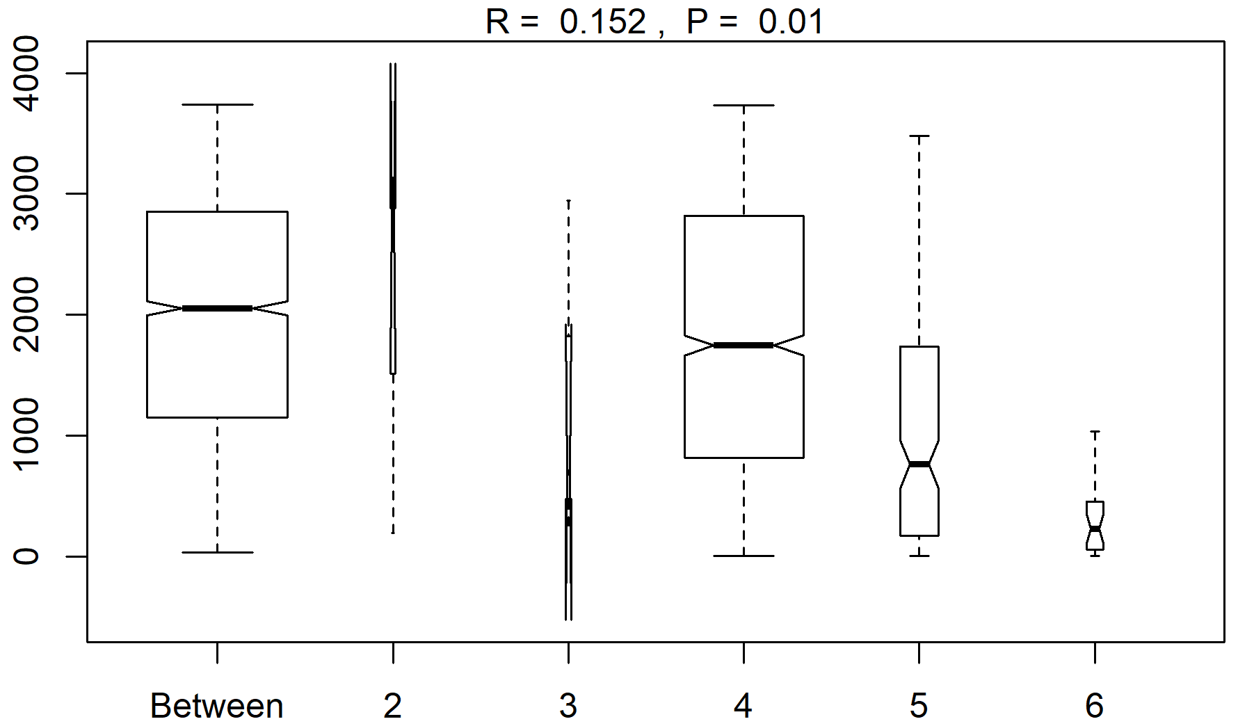
Figure A1 A summary plot from the anosim analysis (testing differences between the sampling areas in species abundances after the NMDS analysis). Range of dissimilarities in the different areas (2–6: station 53, station 54, Astrid Ridge, the 6^∘ E transect and Maud Rise, respectively).

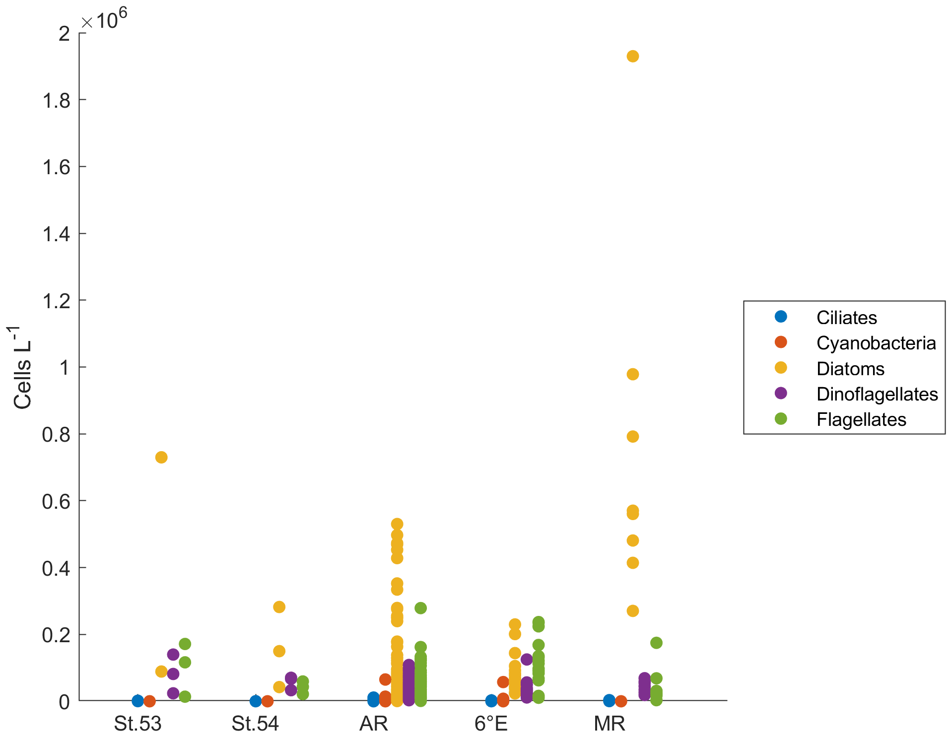
Figure A2 Protist abundance in all samples in the different sampling areas based on microscopy. St.53: station 53, St.54: station 54, AR: Astrid Ridge, 6^∘ E: 6^∘ E transect, MR: Maud Rise.

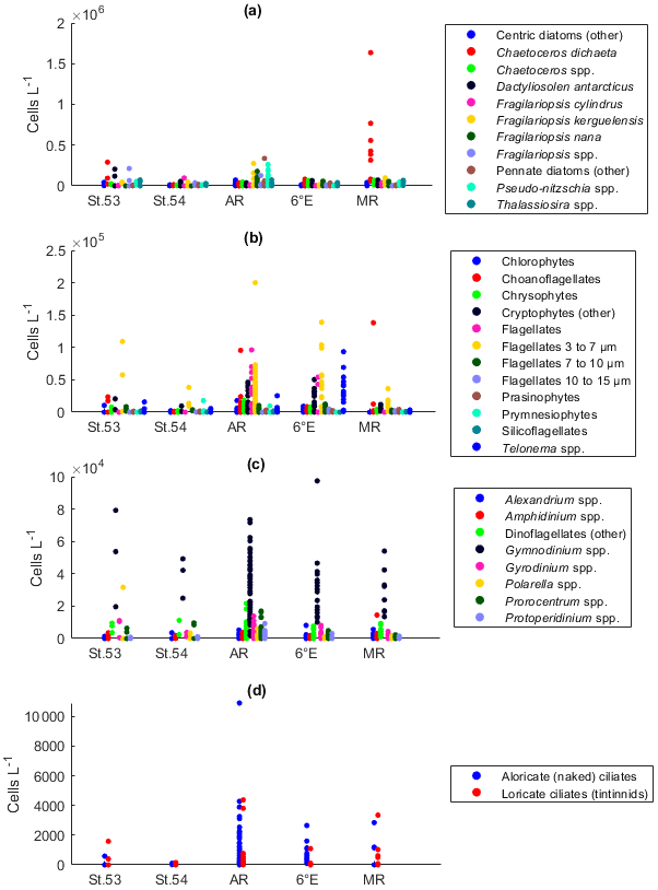
Figure A3 Protist abundance in all samples in the different sampling areas (based on microscopy) for (a) diatoms, (b) flagellates, (c) dinoflagellates and (d) ciliates. St.53: station 53, St.54: station 54, AR: Astrid Ridge, 6^∘ E: 6^∘ E transect, MR: Maud Rise.

Figure A4 Filamentous blue-green algae; cf. Anabaena sp.

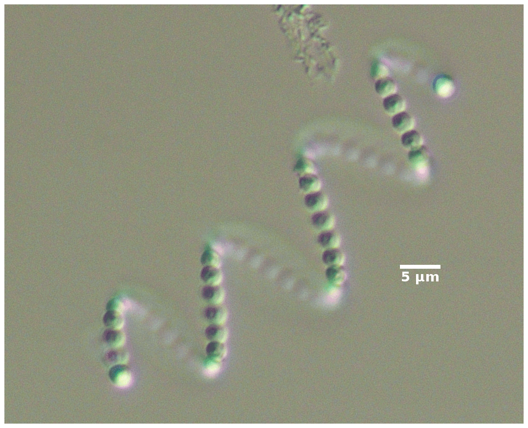
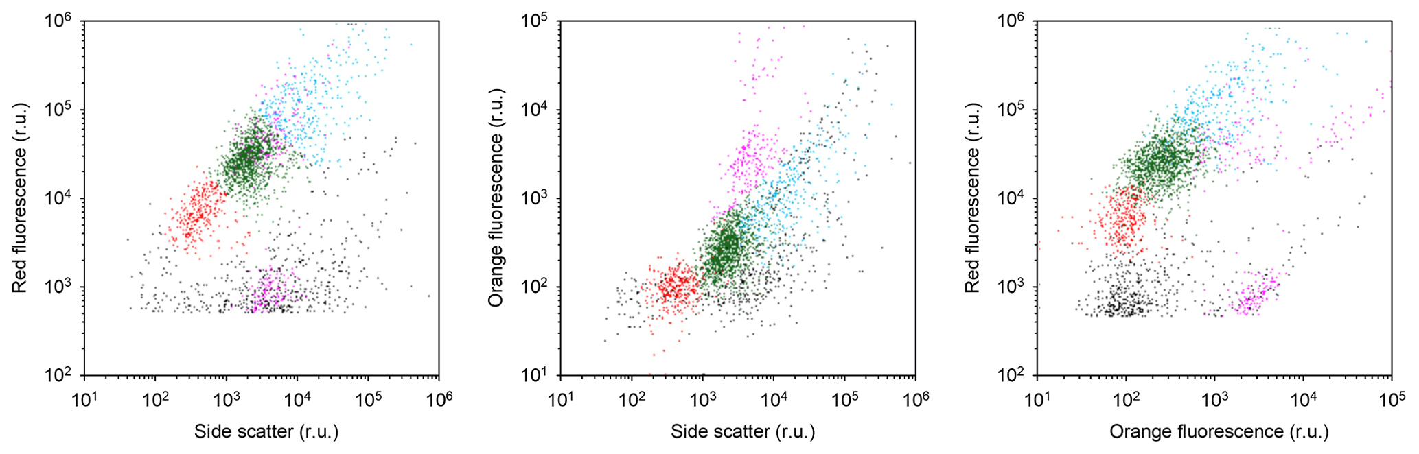
Figure A5 Scatter plots indicating the position of the different phytoplankton populations in the cytograms. Picophytoplankton, Nanophytoplankton 1 and Nanophytoplankton 2 were discriminated based on chlorophyll red autofluorescence versus side scatter (red, green and blue dots, respectively). Possible cyanobacteria and cryptophytes were in addition recognized based on their orange autofluorescence (violet dots). The example shown is from CTD station 61 at 40 m depth. Axes are in relative units (r.u.).

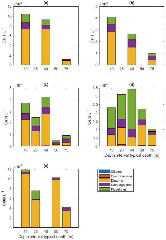
Figure A6 Protist abundances in the different sampling areas averaged per depth interval for (a) station 53, (b) station 54, (c) Astrid Ridge, (d) the 6^∘ E transect, and (e) Maud Rise. Depth intervals (with typical sampling depth in brackets): 5–10 (10), 25–35 (25), 35–45 (40), 50–60, and 65–85 (75) m.

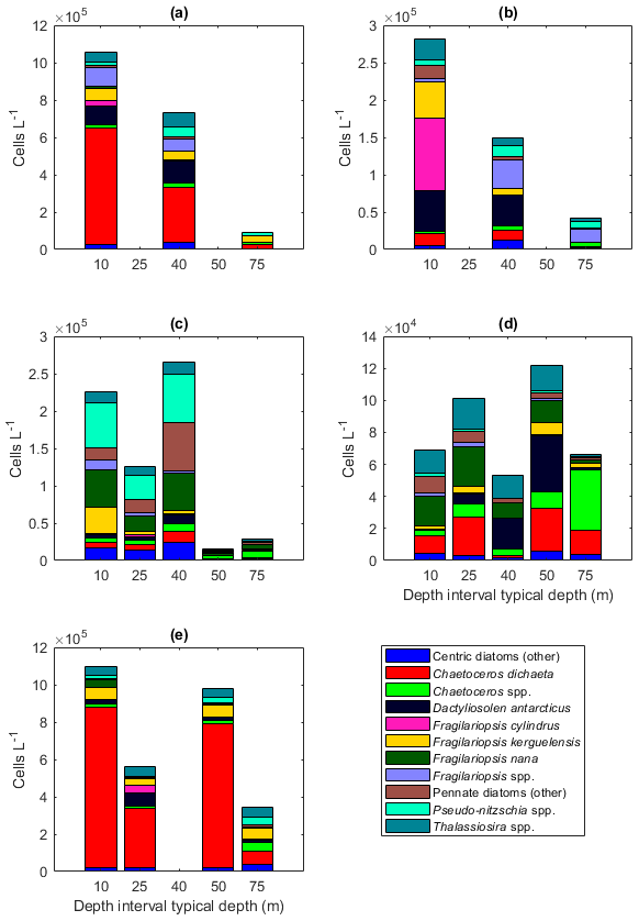
Figure A7 Diatom abundance in the different sampling areas averaged per depth interval for (a) station 53, (b) station 54, (c) Astrid Ridge, (d) the 6^∘ E transect, and (e) Maud Rise. Depth intervals (with typical sampling depth in brackets): 5–10 (10), 25–35 (25), 35–45 (40), 50–60, and 65–85 (75) m.

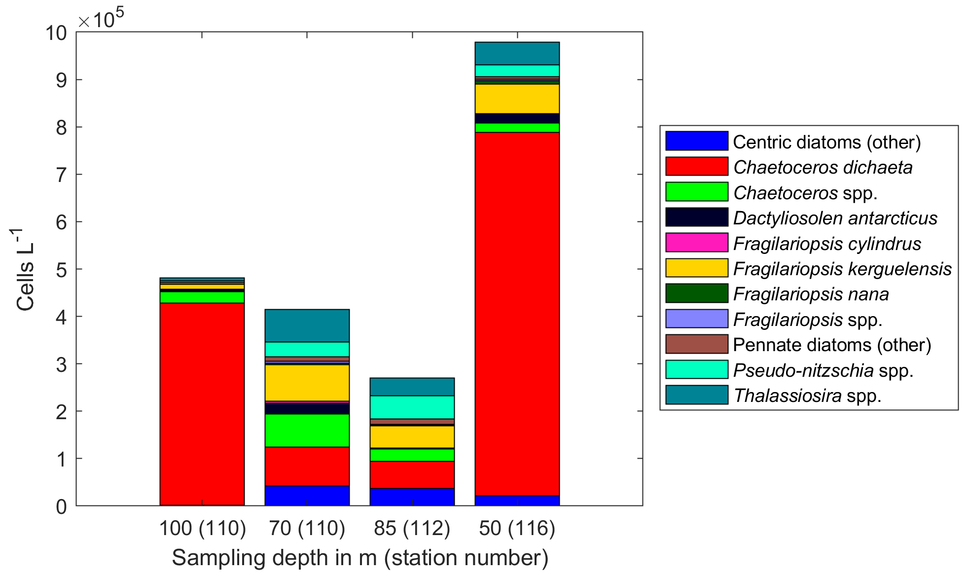
Figure A8 Diatom abundance in available deep samples at Maud Rise. Bars are marked with the sampling depth in meters and the station number in brackets.

Figure A9 NMDS clustering using presence–absence data.

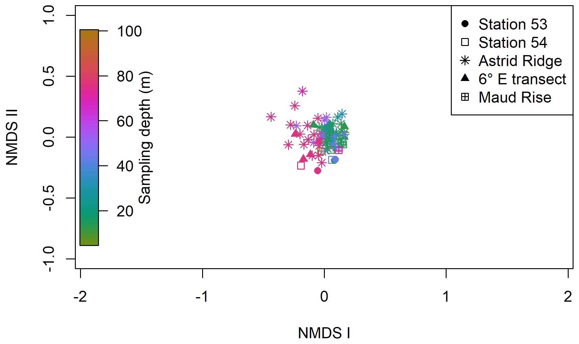
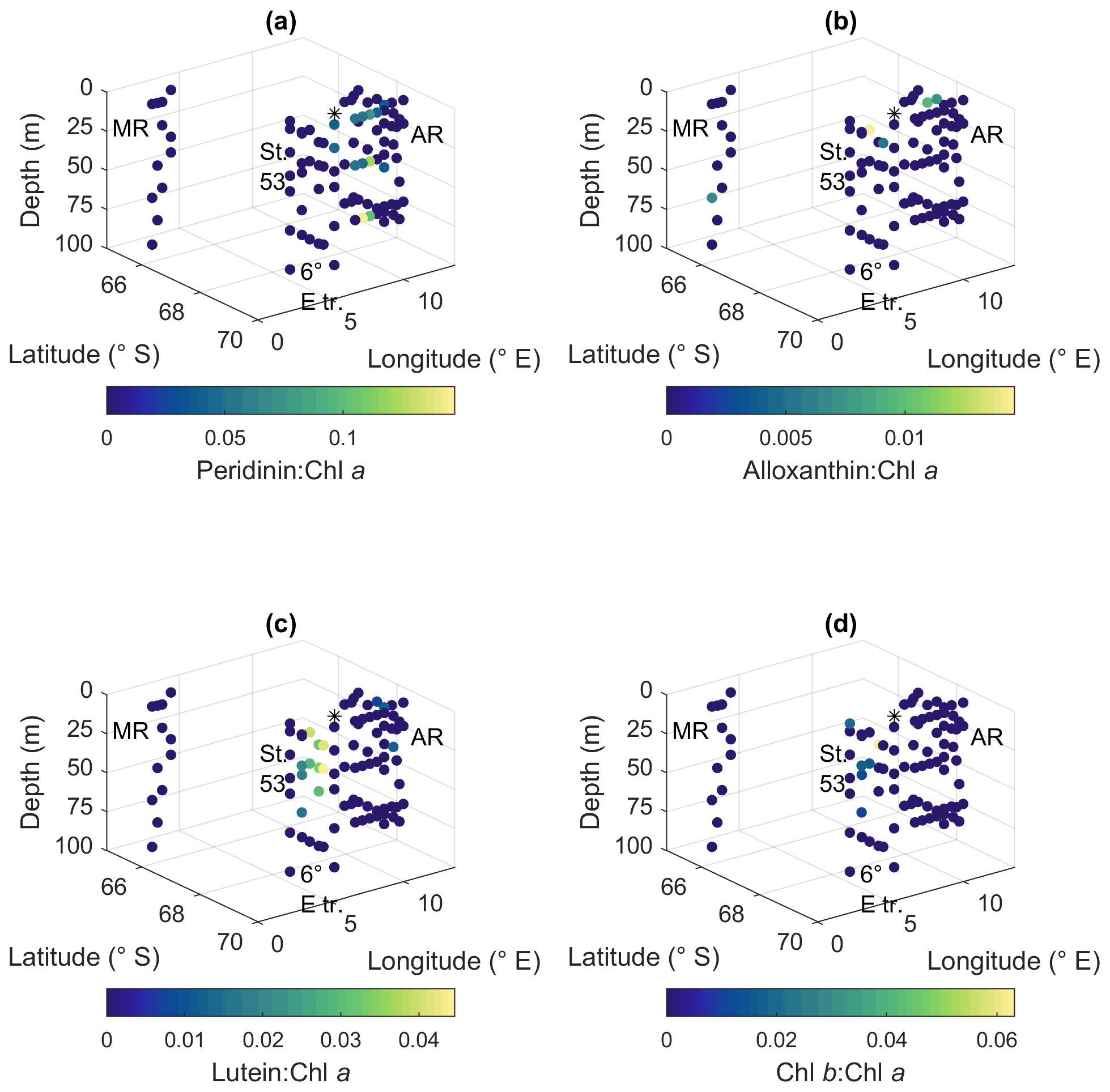
Figure A10 Ratios of algal pigments to Chl a for (a) peridinin, (b) alloxanthin, (c) lutein and (d) Chl b. MR: Maud Rise, St. 53: station 53, AR: Astrid Ridge, 6^∘ E tr.: 6^∘ E transect. Station 54 is marked with a black asterisk.

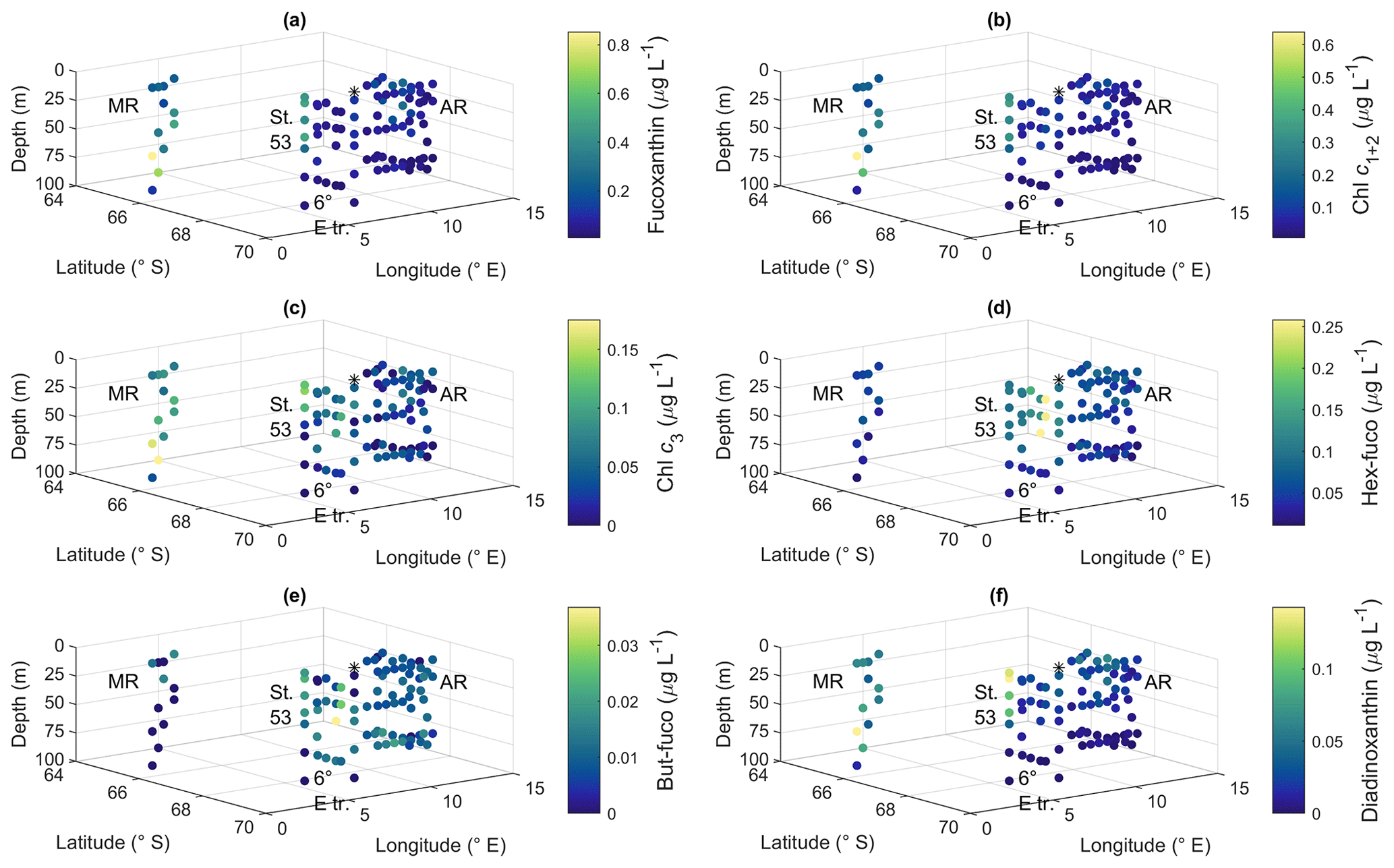
Figure A11 Pigment concentrations of (a) fucoxanthin, (b) Chl c₁₊₂, (c) Chl c₃, (d) hex-fuco, (e) but-fuco and (f) diadinoxanthin. MR: Maud Rise, St. 53: station 53, AR: Astrid Ridge, 6^∘ E tr.: 6^∘ E transect. Station 54 is marked with a black asterisk.

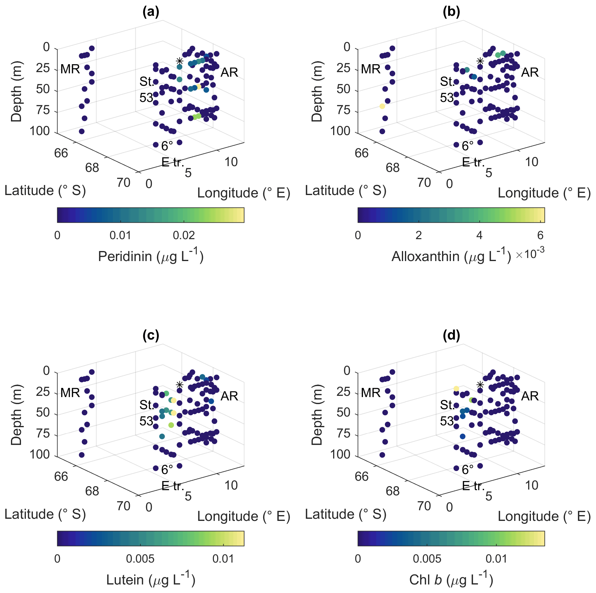
Figure A12 Pigment concentrations of (a) peridinin, (b) alloxanthin, (c) lutein and (d) Chl b. MR: Maud Rise, St. 53: station 53, AR: Astrid Ridge, 6^∘ E tr.: 6^∘ E transect. Station 54 is marked with a black asterisk.

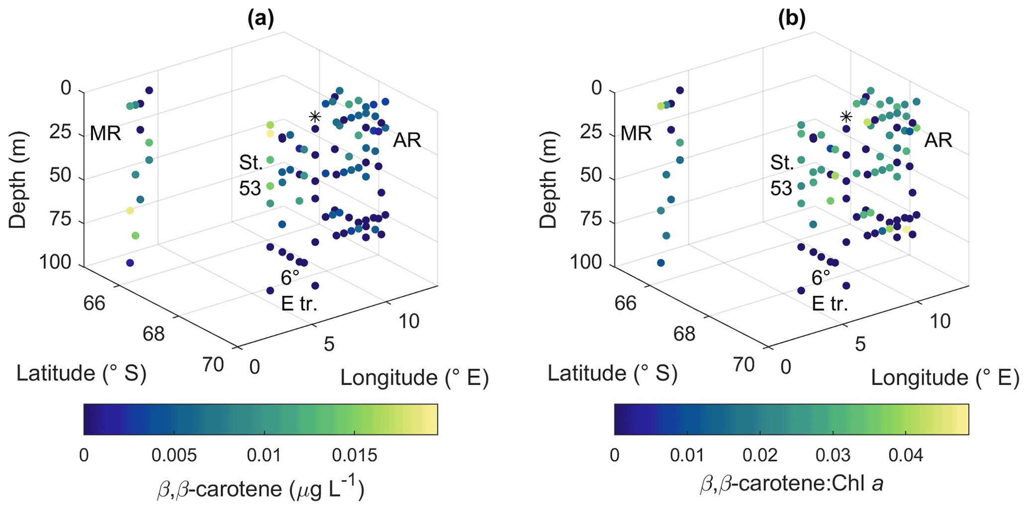
Figure A13 (a) β,β-carotene concentration and (b) ratio of β ,β-carotene to Chl a. MR: Maud Rise, St. 53: station 53, AR: Astrid Ridge, 6^∘ E tr.: 6^∘ E transect. Station 54 is marked with a black asterisk.

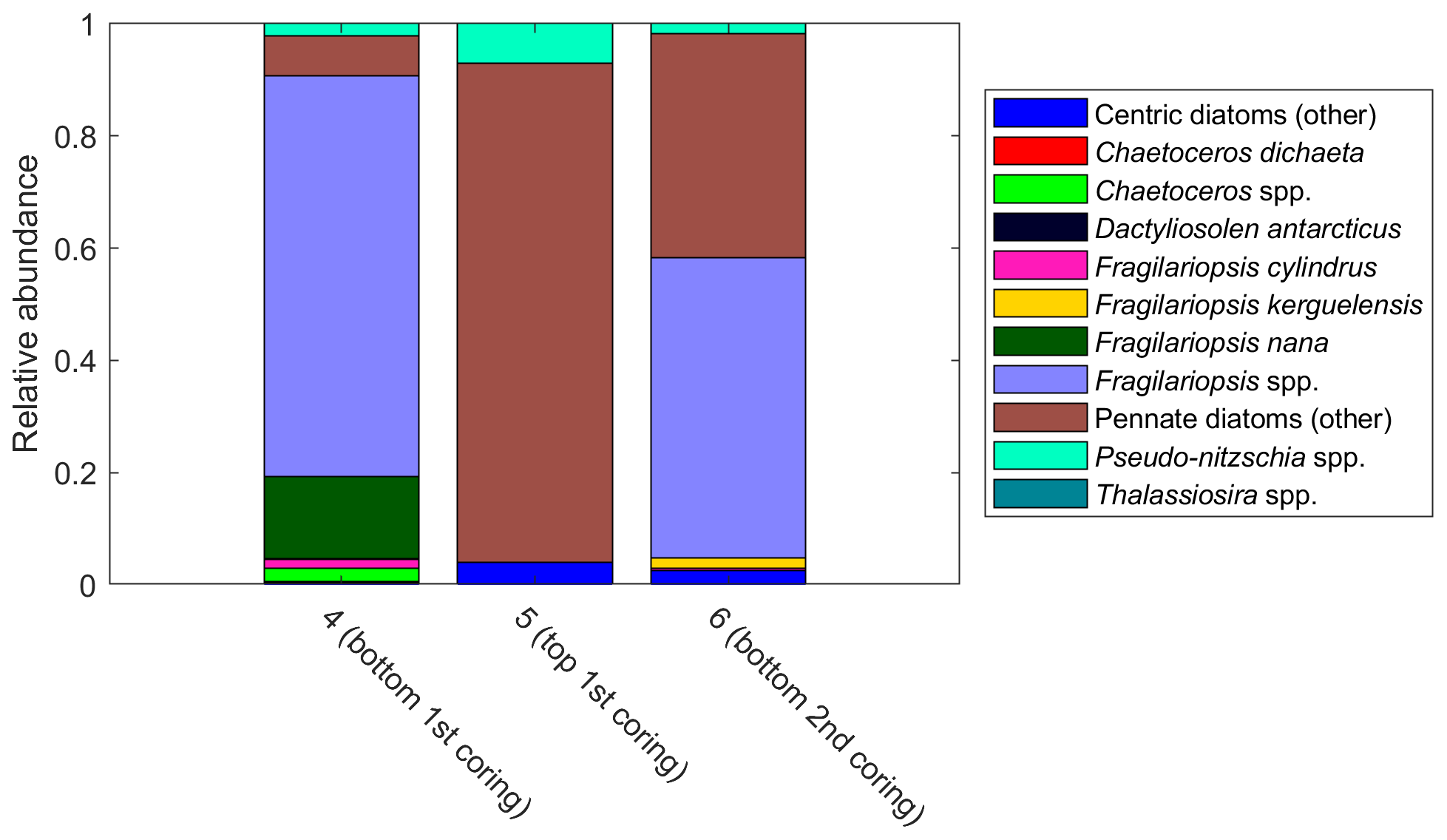
Figure A14 Relative diatom abundance in ice core samples. The colors pink to cyan comprise pennate diatoms. The bars are marked with sample numbers and ice core section explanations. See Table B2 for method descriptions.

Figure A15 (a) Diatom abundance and (b) relative abundance in the south–north transect at 6^∘ E, including station 53 just north of the transect (average abundances per station).

Appendix B: Appendix tables

Table B1 All taxa identified in the CTD station samples down to 100 m (in total 87 samples). For median abundance 2, only the samples where the species/taxon was observed were taken into account (i.e., zero abundances do not contribute to the median value).

Table B2 Initial pigment-to-Chl a ratios used in the CHEMTAX analysis and the final ratio matrices for each cluster (average of the six best-performing runs of the second step; see “Methods”).

Peri: peridinin; Fuco: fucoxanthin; Allo: alloxanthin; Lut: lutein.

Table B3 Comparison of the 20 most abundant diatom species between sea ice samples and Astrid Ridge samples. Species name in bold text indicates presence in both areas.

Two ice floes were sampled along the 6^∘ E transect (the first one on 26 March 2019 at 68.9135^∘ S and 6.0217^∘ E and the second one on 27 March 2019 at 68.4392^∘ S and 5.9135^∘ E). Ice algal taxonomy and abundance samples were taken from a total of three ice core sections: a 10 cm bottom section and an 8.5 cm top section from the 18.5 cm-thick ice core at the first ice floe and a 10 cm bottom section from the 93.5 cm-thick ice core at the second ice floe. A Kovacs 9 cm corer was used, and the ice samples were melted without the addition of filtered seawater in darkness and room temperature and processed as soon as the melting was complete.