the Creative Commons Attribution 4.0 License.
the Creative Commons Attribution 4.0 License.
 | 08 Dec 2022
A coupled ground heat flux–surface energy balance model of evaporation using thermal remote sensing observations
Bimal K. Bhattacharya
Kaniska Mallick
Devansh Desai
Ganapati S. Bhat
Ross Morrison
Jamie R. Clevery
William Woodgate
Jason Beringer
Kerry Cawse-Nicholson
Siyan Ma
Joseph Verfaillie
Dennis Baldocchi
One of the major undetermined problems in evaporation (ET) retrieval using thermal infrared remote sensing is the lack of a physically based ground heat flux (G) model and its integration within the surface energy balance (SEB) equation. Here, we present a novel approach based on coupling a thermal inertia (TI)-based mechanistic G model with an analytical surface energy balance model, Surface Temperature Initiated Closure (STIC, version STIC1.2). The coupled model is named STIC-TI. The model is driven by noon–night (13:30 and 01:30 local time) land surface temperature, surface albedo, and a vegetation index from MODIS Aqua in conjunction with a clear-sky net radiation sub-model and ancillary meteorological information. SEB flux estimates from STIC-TI were evaluated with respect to the in situ fluxes from eddy covariance measurements in diverse ecosystems of contrasting aridity in both the Northern Hemisphere and Southern Hemisphere. Sensitivity analysis revealed substantial sensitivity of STIC-TI-derived fluxes due to the land surface temperature uncertainty. An evaluation of noontime G (Gi) estimates showed 12 %–21 % error across six flux tower sites, and a comparison between STIC-TI versus empirical G models also revealed the substantially better performance of the former. While the instantaneous noontime net radiation (RNi) and latent heat flux (LEi) were overestimated (15 % and 25 %), sensible heat flux (Hi) was underestimated (22 %). Overestimation (underestimation) of LEi (Hi) was associated with the overestimation of net available energy (RNi−Gi) and use of unclosed surface energy balance flux measurements in LEi (Hi) validation. The mean percent deviations in Gi and Hi estimates were found to be strongly correlated with satellite day–night view angle difference in parabolic and linear pattern, and a relatively weak correlation was found between day–night view angle difference versus LEi deviation. Findings from this parameter-sparse coupled G–ET model can make a valuable contribution to mapping and monitoring the spatiotemporal variability of ecosystem water stress and evaporation using noon–night thermal infrared observations from future Earth observation satellite missions such as TRISHNA, LSTM, and SBG.
- Article
(12863 KB) - Full-text XML
- BibTeX
- EndNote


One of the outstanding challenges in evaporation (ET) estimation through surface energy balance (SEB) models concerns an accurate characterization of ground heat flux in the open canopy architecture with mixed vegetation such as savanna or in ecosystems with low mean fractional vegetation cover, prevailing water stress, and strong seasonality in soil moisture. Ground heat flux (G) is an intrinsic component of SEB (Sauer and Horton, 2005), affecting the net available energy for ET (the equivalent water depth of latent heat flux, LE) and sensible heat flux (H). It represents an energy flow path that couples the surface with the atmosphere and has important implications for the underlying thermal regime (Sauer and Horton, 2005). Depending on the vegetation fraction and water stress, the magnitude of instantaneous G varies greatly across different ecosystems. In the humid ecosystems with predominantly dense canopies and high mean fractional vegetation cover, G contributes a small proportion to the surface energy balance. Dense canopy cover leads to less transmission of radiative fluxes through multiple layers of canopies, which results in low warming of the soil floor. Due to persistently high soil water content, humid ecosystems generally show low diurnal and seasonal variability in G. In contrast, the magnitude of G is substantially large in arid and semi-arid ecosystems with sparse and open canopy and soil moisture deficits. Due to the prevailing feedback between the physics of ground heat flux, land–atmosphere interactions, and vegetation ecophysiology, evaporation modeling in the complex ecosystems remains a challenging task (Wang et al., 2013; Kiptala et al., 2013). This paper addresses the challenge of simultaneous estimation of G and ET by combining thermal remote sensing observations with a mechanistic G model and a SEB model.
SEB models mainly emphasize estimating sensible heat flux by resolving the aerodynamic conductance (gA) and computing LE as a residual SEB component as follows.
RN is the net radiation. The proportion of RN that is partitioned into G depends upon soil properties like its albedo, soil moisture, and soil thermal properties such as thermal conductivity and heat capacity, which vary with mineral, organic, and soil water fractions. SEB models use land surface temperature (LST or TS) as an important lower boundary condition for estimating H and LE. Due to the extraordinarily high sensitivity of TS to evaporative cooling and soil water content variations, thermal infrared (TIR) remote sensing is extensively used in large-scale evaporation diagnostics (Kustas and Anderson, 2009; Mallick et al., 2014, 2015a, 2018a; Cammalleri and Vogt, 2015; Anderson et al., 2012). Evaporation estimation through SEB models commonly employs empirical sub-models of G in a stand-alone mode. Despite the utility of mechanistic G models being demonstrated in different studies (Verhoef, 2004; Murray and Verhoef, 2007; Verhoef et al., 2012), no TIR-based evaporation study attempted to couple a mechanistic G model with a SEB model.
The SEB models for ET estimation driven by remote sensing observations generally use linear and nonlinear relationships for estimating G, and such methods generally employ RN, TS, albedo (αR), and NDVI (e.g., Bastiaanssen et al., 1998; Friedl et al., 2002; Santanello and Friedl, 2003). While the inclusion of TS and albedo serves as a proxy for soil moisture and surface characteristic effects in G, inclusion of NDVI provides a scaling of the G–RN ratio for different fractional vegetation covers. Unfortunately, the empirical approaches do not include any information on soil temperature or daily temperature amplitude. These empirical models also lack universal consensus. Setting G as a fraction of RN does not solve the energy balance equation and disregards the role of thermal inertia of the land surface (Mallick et al., 2015b). This could introduce substantial uncertainty in LE estimation because G effectively couples the surface energy balance with energy transfer processes in the soil thermal regime. It provides physical feedback to LE through the effects of soil moisture, temperature, and conductivity (thermal and hydraulic) (Sauer and Horton, 2005). Such feedbacks are most critical in the arid and semi-arid ecosystems, where LE is significantly constrained by the soil moisture dry-down. The limits imposed on LE by the water stress consequently result in greater partitioning of the net available energy (i.e., RN−G) into H and G (Castelli et al., 1999).
When LE is reduced due to soil moisture dry-down, both G and TS tend to show rapid intra-seasonal rise. Therefore, the surface energy balance equation could be linked with the mechanistic G model, TS harmonics (Verhoef, 2004), and soil moisture availability. Realizing the importance of direct estimates of G in LE, and invigorated by the advent of TIR remote sensing, Verhoef et al. (2012) demonstrated the potential of a TI-based mechanistic model (Murray and Verhoef, 2007) (MV2007 hereafter) for spatiotemporal G estimates in semi-arid ecosystems of Africa. Some studies also emphasized the importance of using noontime and nighttime TS and RN for estimating G (Mallick et al., 2015b; Bennet et al., 2008; Tsuang, 2005). The method of MV2007 has so far been tested in a stand-alone mode, and no remote sensing method has so far been attempted to combine such a mechanistic G model (e.g., the MV2007-TI model) with a SEB model for coupled energy–water flux estimation and validation.
By integrating TS into a combined structure of the Penman–Monteith (PM) and Shuttleworth–Wallace (SW) models, an analytical SEB model was proposed by Mallick et al. (2014, 2015a, 2016). The model, Surface Temperature Initiated Closure (STIC), is based on finding an analytical solution for aerodynamic and canopy–surface conductance (gA and gS), where the expressions of the conductances were constrained by an aggregated water stress factor. By physically linking water stress (TS-derived) with gA and gS, STIC established direct feedback between TS, H, and LE and simultaneously overcame the need for empirical parameterization to estimate the conductances (Mallick et al., 2016, 2018a). Different versions of STIC have been extensively validated in different ecological transects (tropical rainforest to woody savanna) and aridity gradients (humid to arid) (Trebs et al., 2021; Bai et al., 2021; Mallick et al., 2015a, 2016, 2018a, b; Bhattarai et al., 2018, 2019). Based on the conclusions of Verhoef et al. (2012), Mallick et al. (2014, 2015a, b, 2016, 2018a, b, 2022), Bhattarai et al. (2018, 2019), and Bai et al. (2021), there is a need to address some of the challenges in SEB modeling, which are (i) accurate estimation of G and ET in sparse vegetation, (ii) testing of the utility of coupling a TI-based G model with an analytical SEB model for accurately estimating G and ET, and (iii) detailed evaluation of a coupled G–SEB model at the ecosystem scale. Realizing the significance of the mechanistic G model (MV2007) and the advantage of the analytical STIC model and to mitigate some of the overarching gaps in SEB modeling in sparsely vegetated open canopy systems, this study presents the first-ever coupled implementation of MV2007 G with the most recent version of STIC (STIC1.2). We name this new coupled model STIC-TI, and it requires noon–night TS and associated remotely sensed land surface variables as inputs. We performed subsequent evaluation of STIC-TI in nine terrestrial ecosystems in arid, semi-arid, and sub-humid climates in India, the United States of America (USA) (Northern Hemisphere), and Australia (Southern Hemisphere) at the eddy covariance flux tower sites. The current study addresses the following research questions and objectives.
- i.
What is the performance of STIC-TI G estimates when compared with conventionally used empirical G models in ecosystems with low mean fractional vegetation cover (fc) (≤0.5) and with larger soil exposure to radiation, for example, in savanna?
- ii.
How do the estimates from STIC-TI LE and H fluxes compare with LE and H observations in diverse terrestrial ecosystems that represent a varied range of fc (0.25–0.5) covering cropland, savanna, and mulga vegetation (woodlands and open forests dominated by the mulga tree – Acacia aneura) spread across arid, semi-arid, sub-humid, and humid climates over a vast range of rainfall (250 to 1730 mm), temperature (−4 to 46 ∘C), and soil regimes?
- iii.
What is the seasonal variability of G and evaporative fraction from the STIC-TI model in a wide range of ecosystems having contrasting aridity and vegetation cover?
It is important to mention that assessing the performance of STIC-TI LE and H with respect to other SEB models is not within the scope of the present study. The prime focus of the current study is to assess the sensitivity of STIC-TI, temporal variability of the retrieved SEB fluxes, and cross-site validation of the individual SEB components.
A list of the variables, their symbols, and the corresponding units is given in Appendix A.
2.1 Study site characteristics
The present study was conducted using data from nine flux tower sites (four sites in India; three sites in Australia; two sites in the USA) equipped with eddy covariance (EC) measurement systems. The distribution of the flux tower sites considered for the present study are shown in Fig. 1 below. The sites cover a wide range of climates, vegetation types, a low fractional vegetation cover (fc) of around 0.5, and contrasting aridities (Table 1). In India, a network of EC towers was set up under the Indo-UK INCOMPASS (INteraction of Convective Organization and Monsoon Precipitation, Atmosphere, Surface and Sea) program (Turner et al., 2019) at Jaisalmer (IND-Jai) in Rajasthan state, Nawagam (IND-Naw) in Gujarat state, and Samastipur (IND-Sam) in Bihar state and under the Newton Bhabha program (Morisson et al., 2019a, b) at Dharwad (IND-Dha) in Karnataka state. The flux footprint for EC towers in India varied from 500 m to 1 km (Bhat et al., 2019). In the present study, about 90 % of the fluxes came from an area within 500 m to 1 km of the EC tower. Therefore, the relative contribution of vegetated land surface area to the fluxes is close to 90 % (Schmid, 2002; Vesala et al., 2008). The remaining percentage of fluxes originated from an area beyond the flux footprint. The mean annual fc was found to vary from 0.25 to 0.52, with a standard deviation (SD) ranging from 0.1 to 0.16.
The IND-Jai site represents the arid western zone over desert plains of the natural grassland ecosystem. The region receives very low rainfall (100–300 mm) during monsoon and experiences a wide range in air temperature, high solar radiation, wind speed, and high evaporative demand (Raja et al., 2015). The IND-Naw site represents a semi-arid agroecosystem in the middle Gujarat agroclimatic zone of northwestern India and has a pre-dominant rice–wheat cropping system. The IND-Sam site has a sub-humid climate of the northwestern alluvial plain zone in the Indo-Gangetic Plain (IGP) situated in eastern India, and this site also follows rice–wheat crop rotation. IND-Dha represents the humid sub-tropical climate of the transition zone in southern India, and this site is comprised of crops.
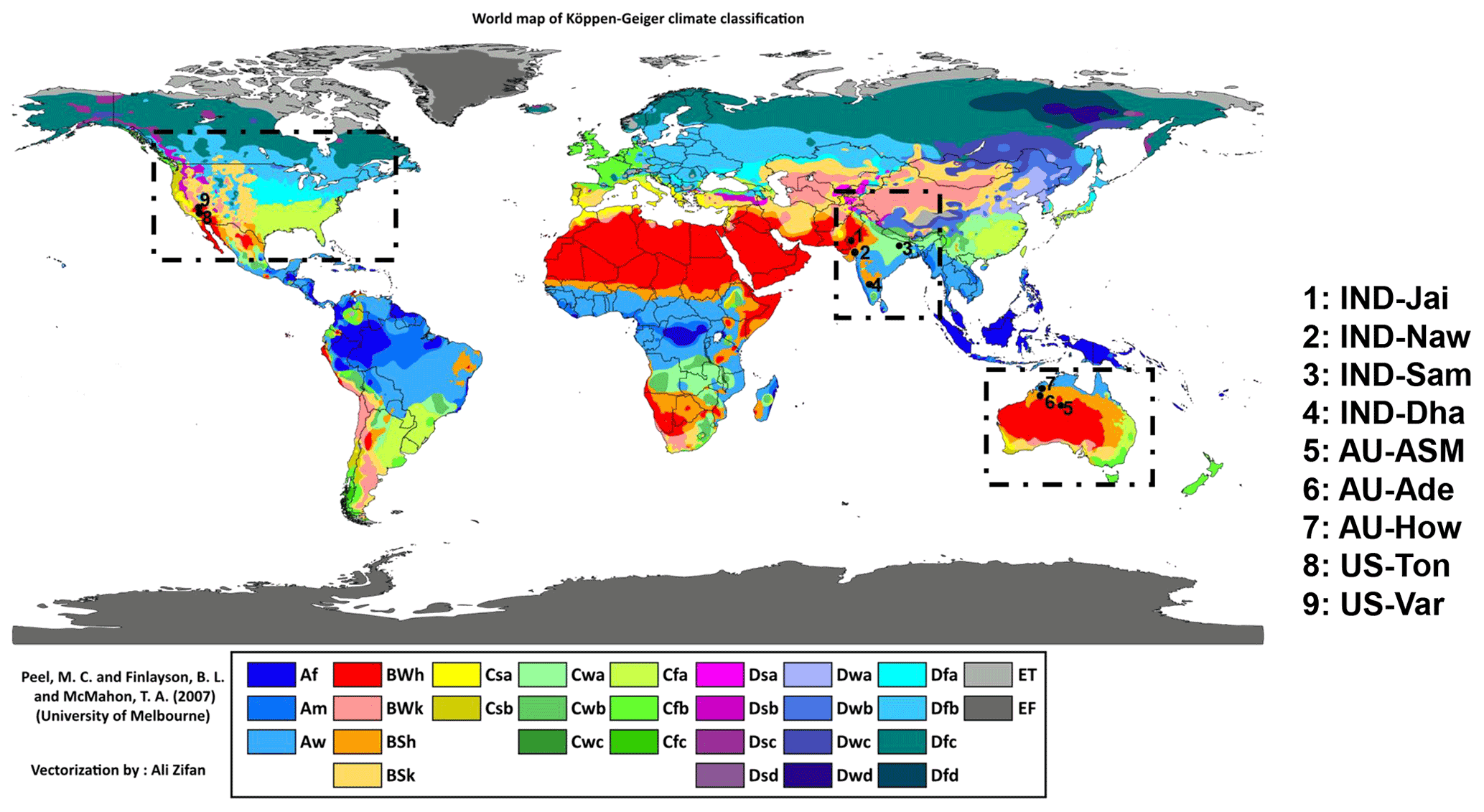
Figure 1Locations of the flux tower sites in India, Australia, and the USA overlaid on a climate-type map. Image source: Peel et al. (2017).
In the USA, two EC tower sites were located at Tonzi Ranch (US-Ton) and Vaira Ranch (US-Var), in the lower foothills of the Sierra Nevada. Both EC stations are part of the AMERIFLUX Management Project (https://ameriflux.lbl.gov/, last access: 3 December 2022). US-Ton is classified as an oak savanna woodland. While the overstorey is dominated by blue oak trees (40 % of the total vegetation) with intermittent grey pine trees (3 trees ha−1), the understorey species include a variety of grasses and herbs. The mean annual rainfall at this site is 559 mm. US-Var is a grassland-dominated site, and the growing season is confined to the wet season only, typically from October to early May. The mean annual rainfall at this site is 559 mm. The mean annual fc was found to vary from 0.18 to 0.26, and SD is of the order of 0.06 to 0.07.
In Australia, three EC tower sites were located at Howard Springs (AU-How), Alice Springs Mulga (AU-ASM), and Adelaide River (AU-Ade) in the Northern Territory as part of the OzFlux network (Beringer et al., 2016) and the Terrestrial Ecosystem Research Network (TERN), which is supported by the National Collaborative Infrastructure Strategy (NCRIS) (http://www.ozflux.org.au/monitoringsites/index.html, last access: 3 December 2022). AU-How is situated in the Black Jungle Conservation Reserve representing an open woodland savanna, and the mean annual rainfall is 1750 mm. The AU-ASM is located at Pine Hill cattle station near Alice Springs. The woodland is characterized by a mulga canopy, and mean annual rainfall is 306 mm. AU-Ade represents savanna with a mean annual rainfall of 1730 mm. The mean annual fc varied from 0.21 to 0.48 with an SD range of 0.08–0.17. A description of Australian flux sites is given in Beringer et al. (2016). Average heights of vegetation are 1.15 m at IND-Naw, 1 m at IND-Jai, 1.23 m at IND-Sam, 1.5 m at IND-Dha, 6.5 m at AU-ASM, 15 m at AU-How, 7 m at AU-Ade, 10 m at US-Ton, and ≤0.5 m at US-Var.
Table 1An overview of the eddy covariance flux tower site characteristics used in the present study.
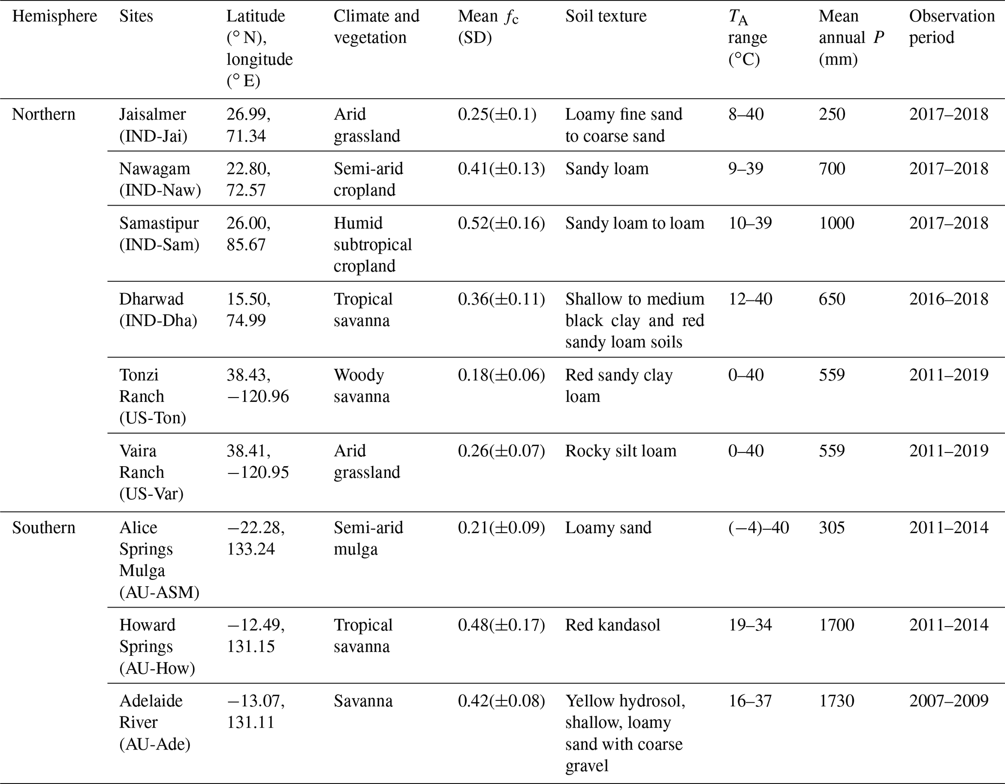
TA: air temperature during the observation period. P: rainfall (mm) measured using the rain gauge at the flux tower site during the study period. IND is for India, AU is for Australia, and US is for the United States. SD is the standard deviation of the annual mean fc which is computed from the NDVI as mentioned in Sect. 3.1.
2.2 Datasets
2.2.1 Micrometeorological data at flux tower sites
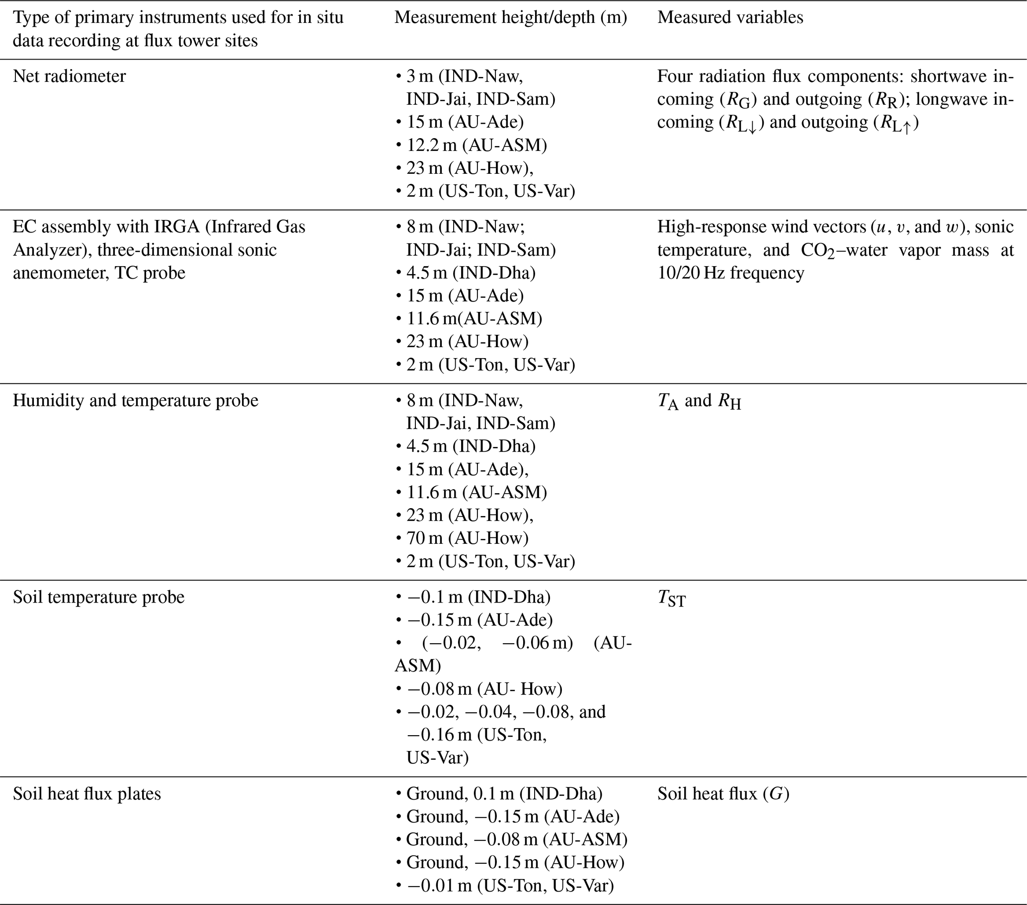
Standardized, controlled, and harmonized SEB flux and meteorological data from nine EC towers were used in the present analysis. In Australia, H and LE were measured through the EC systems and RN was measured through net radiometers at varying heights of 15 m (AU-Ade), 23 m (AU-How), and 11.6 m (AU-ASM), respectively. In India, the EC measurement height was maintained approximately at 8 m above the surface, except at IND-Dha, where it was installed at a height of 4.2 m. In the USA, the SEB measurements were carried out at tower heights of 23 m at US-Ton and 2 m US-Var. A summary of the instrumentation is given in Table A2 of Appendix A. All the flux tower sites were equipped with a range of meteorological instrumentation which measured diurnal air temperature (TA) and relative humidity (RH), four components of the net radiation (RN, consisting of downwelling and upwelling shortwave and longwave radiation: SW ↓, SW ↑, LW ↑ and LW ↓, respectively) above the vegetated canopy. In addition, the diurnal soil heat flux (G) and soil temperature (TST) were measured at all three Australian sites and both US sites. In India, the diurnal soil heat flux was measured only at IND-Dha.
For the Indian sites, the raw EC measurements of the turbulent wind vectors (u, v, and w, for horizontal, meridional, and vertical, respectively), sonic temperature (T), and CO2 and water vapor mass density were recorded at a sampling rate of 20 Hz. Raw EC data were post-processed to obtain level-3 quality-controlled and harmonized surface fluxes at 30 min flux-averaging intervals using the EddyPRO® Flux Calculation software (LI-COR Biosciences, Lincoln, Nebraska, USA) using the data-handling protocol described by Bhat et al. (2019). The EC data from the OzFlux sites were averaged over 30 min recorded by the logger and processed through levels using the PyFluxPro standard software processing scripts as mentioned in Isaac et al. (2017). Level 3 (L3) used in this paper was produced using PyFluxPro (Isaac et al., 2017) employing Dynamic INtegrated Gap filling and partitioning for the Ozflux (DINGO) system as described in Donohue et al. (2014) and Beringer et al. (2016). The quality-checked EC data at 30 min intervals for the two AMERIFLUX sites US-Ton and US-Var were acquired from https://doi.org/10.17190/AMF/1245971 and https://doi.org/10.17190/AMF/1245984, respectively.
2.2.2 Remote sensing data
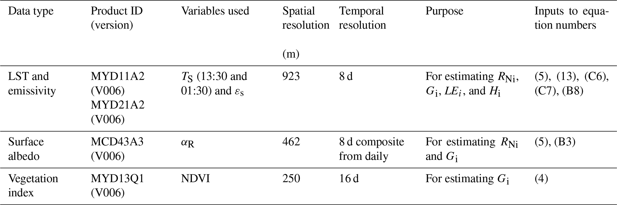
Optical and thermal remote sensing observations available from the Moderate Resolution Imaging Spectroradiometer (MODIS) (Didan, 2015) onboard the Aqua platform were used in the present study (Table 2) for estimating G and its associated SEB fluxes. These include 8 d land surface temperature (LST or TS) at 13:30 and 01:30, surface emissivity (εs) (MYD11A2), daily surface albedo (αR) (MCD43A3), and 16 d NDVI (MYD13A2). The overpass times of MODIS Aqua are at 13:30 and 01:30. The 8 d average values of clear-sky TS available from MYD11A2 data were used (source: https://vip.arizona.edu/documents/viplab/MYD11A2.pdf, last access: 3 December 2022) for all nine flux tower sites. Since the MYD21A2 LST product is known to provide better accuracy (1–1.5 K) (Hulley et al., 2016) as compared with the MYD11A2 LST over semi-arid and arid ecosystems, the former was also used in STIC-TI to compare LE and H estimates (see Table 5 in Sect. 4.4) with the estimates of the MYD11A2 LST over the arid and semi-arid sites (IND-Jai, IND-Naw, US-Ton). The noon–night pair of thermal remote sensing observations from Aqua are close to the times of occurrences of maximum and minimum soil surface temperature (see Fig. 2) and are therefore ideal for soil heat flux modeling using thermal inertia. The MODIS Terra overpass times are at 11:00 and 23:00 and are far from the times of occurrences of minimum–maximum soil temperatures. Therefore, MODIS Aqua acquisition times were used in the present study.
Table 2A summary of MODIS Aqua optical and thermal remote sensing products used in the present study.
3.1 Coupled soil heat flux–SEB model
In this paper, we modified a thermal inertia (TI)-based soil heat flux (G) model using noon–night thermal remote sensing observations and thereafter coupled the TI-based G with STIC1.2. A clear-sky net radiation (RN) model was also introduced into this coupled model, and the RN estimation algorithm is described in Appendix B. The estimation of G by modifying the MV2007-TI approach and its coupling with STIC1.2 is the most novel component of the modeling scheme, and it is therefore described in the main body of the paper (Sect. 3.1.1). Such a coupling enabled the implementation of a mechanistic G model along with an analytical SEB model using optical–thermal remote sensing data. The coupled model is hereafter referred to as STIC-TI.
3.1.1 MV2007 soil heat flux model based on TI
The functional form for estimating instantaneous G (Gi hereafter) (Eq. 2 below) is based on the harmonic analysis of soil surface temperature and is described in detail by Murray and Verhoef (2007) and Maltese et al. (2013).
Gi is the soil heat flux at the surface at a particular instance (W m−2); Γ is the soil thermal inertia (J m−2 K−1 s−0.5), k is the total number of harmonics used, A is the amplitude (∘C) of the nth soil surface temperature (TST) harmonic, ω is the angular frequency (rad s−1), t is the time (s), is the phase shift of the nth soil surface temperature harmonic (rad), JS is the summation of harmonic terms of soil surface temperature (K), and Δt (s) is the time offset between the canopy composite temperature and the below-canopy soil surface temperature. Here, we represent Gi and A as ecosystem-scale (≤1 km) soil heat flux and surface soil temperature amplitude (averaged from the soil surface to 10 cm depth), respectively, and assume it to be valid for a different vegetated landscape.
Since we have considered a single pair (noon–night corresponding to 13:30 and 01:30) of MODIS Aqua LST data in the present study, the phase shift () is taken as 0, and the number of harmonics is taken as 1 (k=1) for estimating Gi. Thus, Eq. (2) is modified as follows,
with the two boundary values (i.e., Δt=1.5 h for fc=1 and Δt=0 for fc=0, fc being the vegetation fraction), and a linear approach is proposed here to describe the time offset Δt as a function of fc (Maltese et al., 2013). For a given day, fc was derived by normalizing NDVI with the upper–lower limits of the annual NDVI cycle.
Scaling function for estimating ecosystem-scale surface soil temperature amplitude (A)
Estimating ecosystem-scale A involves two steps, (a) computing point-scale soil surface temperature amplitude (from the surface to 0.1 m depth) (TSTA hereafter) from the available measurements of soil surface temperature and (b) linking TSTA with remote sensing variables to develop scaling functions for A. Point-scale soil temperature measured at different depths within the top 10 cm soil layer at AU-ASM, US-Ton, and US-Var was averaged and considered to be a representative surface soil temperature (0–10 cm). For Ind-Dha and AU-Ade, single-depth (10 cm) soil temperature measurement was used. Studies also showed that LST carries some signal beneath the skin of the surface (Johnston et al., 2022).
Several studies suggested a theoretical sinusoidal trajectory of soil surface and sub-surface temperatures (Gao et al., 2010), where the amplitude is maximum at the surface, and it gradually decreases with depth to become 37 % of the surface amplitude until the damping depth (Hillel, 1982). However, at deeper depths, soil temperatures remain constant with time and do not show many fluctuations as compared with surface or near-surface soil temperatures. This invariant soil temperature is called deep soil temperature (Mihailovic et al., 1999). However, the diurnal surface soil temperature measurements (within the top 0.1 m depth) across different flux tower sites showed a sinusoidal–exponential behavior, i.e., a sinusoidal pattern from sunrise until the afternoon and an exponential pattern from afternoon through sunset to the next sunrise. An illustrative example of the theoretical and observed trajectories of surface soil temperature is shown in Fig. 2. This diurnal surface soil temperature variation has a single harmonic component (Gao et al., 2010). To compute TSTA, a theoretical half-curve of the sinusoidal pattern is assumed and was derived from measurements as exemplified in Fig. 2.
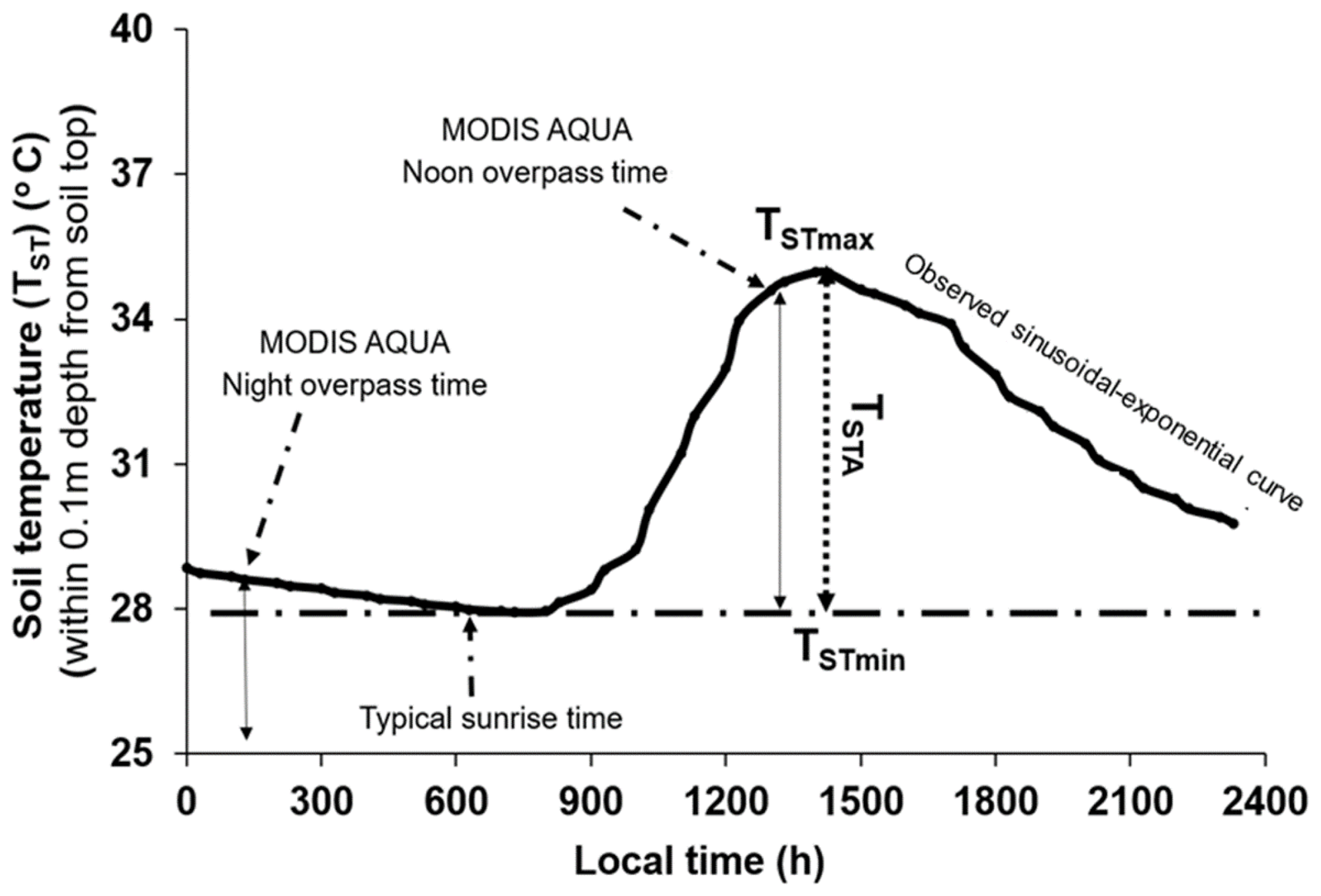
Figure 2An illustrative example of the typical diurnal variation of observed soil temperature (TST) (from the surface to 0.1 m depth) at OzFlux sites and timings of MODIS AQUA observations. Here, TSTmax and TSTmin are maximum and minimum point-scale observed soil surface temperatures.
It is evident from Fig. 2 that TSTmin represents the minimum surface soil temperature occurring 1–1.5 h after sunrise, and TSTmax occurs during 12:30–15:00 local time. The in situ measured TST on completely clear-sky days at OzFlux sites was used to extract TSTmax and TSTmin, and TSTA was derived as TSTmax–TSTmin from the theoretical half-curve of the sinusoidal pattern.
TSTA is generally influenced by several land surface characteristics such as surface temperature and surface albedo of the soil–canopy complex, surface heat capacities, fractional canopy cover, and thermal conductivity. TS and αR are the major thermal and reflective land surface properties that have strong synergy with surface soil temperature dynamics. Hence, we have used bivariate regression analysis to develop a scaling function for estimating ecosystem-scale TSTA (top to 0.1 m depth). The bivariate regression is based on the difference of noon (d) and night (n) TS data and αR (Duan et al., 2013; Tian et al., 2014) from MODIS Aqua. The scaling function given in Eq. (5) estimates ecosystem-scale TSTA (symbolized as “A” in Eq. 5) from the surface to 0.1 m soil depth:
Here, B1, B2, and B3 are coefficients of the regression model. TSd and TSn are noontime and nighttime LST, respectively. The results of this regression analysis are elaborated on in Sect. 4.1.
Estimating Γ
Γ is the key variable for estimating Gi using Eq. (2). MV2007 adopted the concept of normalized thermal conductivity (Johansen, 1975) and developed a physical method to estimate Γ as follows:
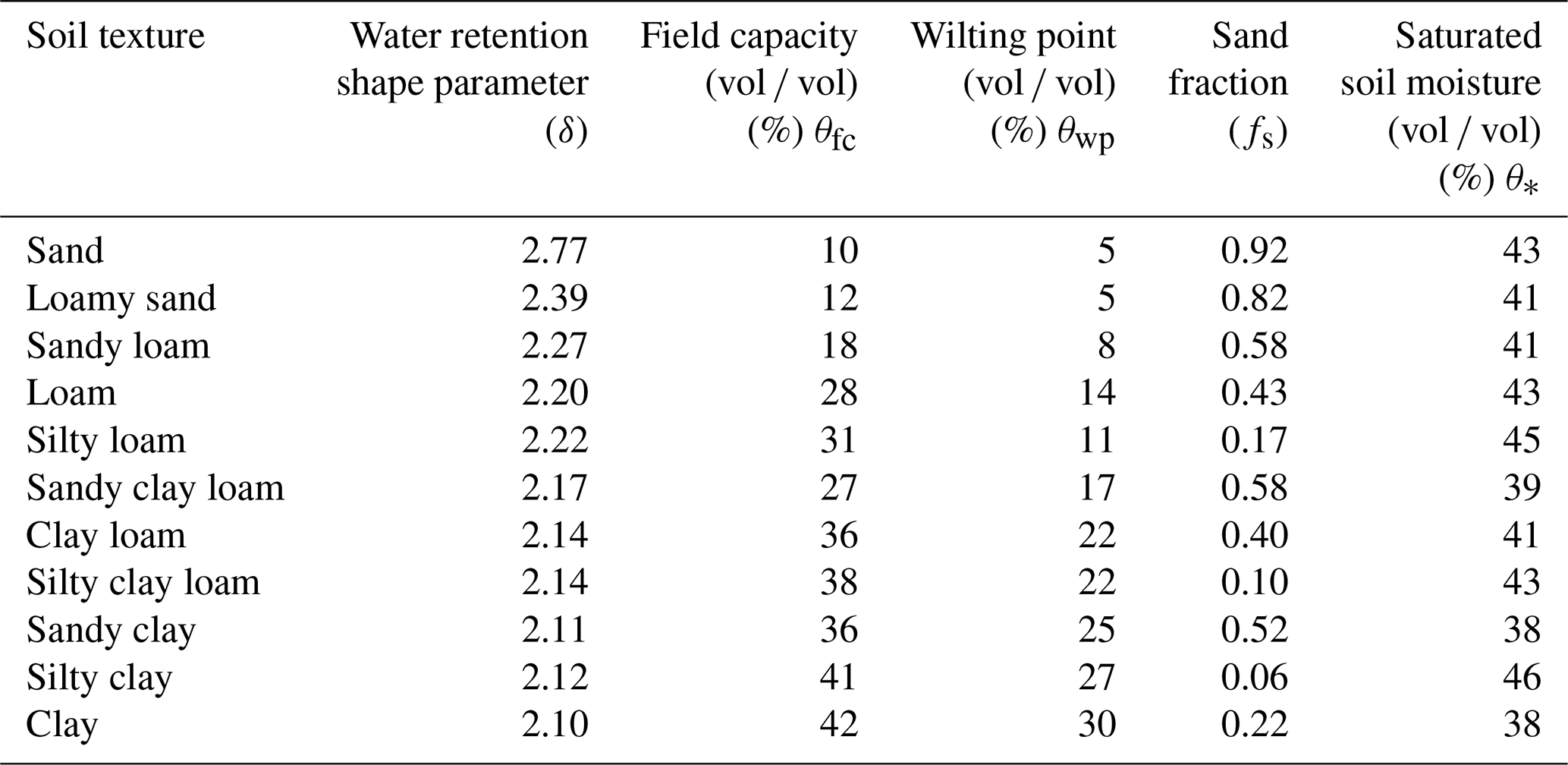
where τ∗ and τ0 are the thermal inertia for saturated and air-dry soil (J m−2 K−1 s−0.5), ; , Υ′ (unitless) is a parameter depending on the soil texture (Murray and Verhoef, 2007; Minasny and Hartemink, 2011; Anderson et al., 2007), Sr (m3 m−3) is relative saturation and is equal to (), and δ (unitless) is the shape parameter which is dependent on the soil texture. θ∗ (m3 m−3) is the soil porosity (equal to the saturated soil moisture content when the soil moisture suction is zero), θ (cm3 cm−3) is the volumetric soil moisture, and D1, D2, and D3 are coefficients which were derived from a large number of experimental data. The reported global values of D1, D2, and D3 were taken as −1062.4, 1010.8, and 788.2, respectively (Maltese et al., 2013). The values for θ∗ and the shape parameter for soil textures across the study sites were specified according to Van Genuchten (1980). The details are mentioned in Table E1 of Appendix E.
In the present study, the relative soil moisture saturation, , is represented in terms of an aggregated moisture availability (M) of the canopy–soil complex through a linear function (Eq. 12). In the case of zero canopy cover, M represents the soil moisture availability from the surface to 0.1 m depth. In the sparse and open canopy, rates of moisture availability from soil to root and root to canopy were assumed to be the same.
Theoretically, M is expressed as the available soil moisture fraction between field capacity (θfc) and the permanent wilting (θwp) point as given in Eq. (7) below.
where θfc (m3 m−3) is the volumetric soil moisture at the field capacity (at a suction of 330 hPa), and θwp (m3 m−3) is the volumetric soil moisture at the permanent wilting point (at a suction of 15 000 hPa). Since θfc, θ∗, and θwp are characteristic volumetric soil moisture contents corresponding to specific suctions and depend on the soil texture, dividing the numerator and denominator in Eq. (7) by θ∗ gives the following expression:
Due to their dependence on soil texture, the ratios () and () are treated as constants. These are represented as C and C′ in the later equations (Eqs. 9, 10, and 11). The constants C and C′ vary from 0.3 to 0.8 and from 0.1 to 0.4 (Murray and Verhoef, 2007; Minasny and Hartemink, 2011; Anderson et al., 2007), respectively, over different soil textures.
By replacing Sr in Eq. (6) as and by rearranging Eq. (10), the following linear function is obtained.
Thus, the modified equation to calculate Γ is given by Eq. (12) as follows:
By substituting the values obtained from Eqs. (4), (5), and (12) into Eq. (3), we obtained the instantaneous ecosystem-scale Gi corresponding to the MODIS Aqua noontime overpass. The intrinsic link between Gi estimates through MV2007-TI and the SEB scheme in STIC1.2 is made through M, where the computation of M follows the procedure as described in Mallick et al. (2016, 2018a, b) and Bhattarai et al. (2018) (description in Appendix C).
Estimating M
In STIC1.2, an aggregated moisture availability (M) of the canopy–soil complex is expressed as the ratio of the “vapor pressure difference” between the aerodynamic roughness height of the canopy (i.e., source/sink height) and air to the “vapor pressure deficit” between aerodynamic roughness height and the atmosphere:
where e0 and are the actual and saturation vapor pressure at the source/sink height, eA is the atmospheric vapor pressure, is the saturation vapor pressure at the surface, T0D is the dew-point temperature at the source/sink height, TS is the LST, TD is the air dew-point temperature, s1 and s2 are the psychrometric slopes of the saturation vapor pressure and temperature between the (T0D−TD) versus (e0−eA) and (TS−TD) versus () relationship, and κ is the ratio between () and (). To solve Eq. (13), estimation of T0D is necessary. An initial estimate of and M was obtained following Venturini et al. (2008), where s1 and s3 were approximated in TD and TS, respectively. However, Eq. (13) cannot be solved directly because there are two unknowns in one equation. However, since T0D also depends on LE (Mallick et al., 2016, 2018a), an iterative update of T0D (and M) was carried out by expressing T0D as a function of , which is described in detail by Mallick et al. (2016, 2018a) and Bhattarai et al. (2018). In the numerical iteration, s1 was not updated to avoid numerical instability, and it was expressed as a function of TD.
3.1.2 STIC-TI: coupling the modified MV2007-TI and STIC 1.2
The initiation of the coupling between MV2007-TI and STIC1.2 was executed by linking Gi estimates from the modified MV2007-TI with M estimates from STIC1.2. Having the initial estimates of M (through Eq. 13), an initial estimation of Gi was made from Eq. (2), where Sr in Eq. (11) was replaced with the initial estimates of M′. From the initial estimates of Gi (Eq. 2) and RNi (equations in Appendix B), initial estimates of LEi and Hi were obtained through the Penman–Monteith energy balance (PMEB) equation. Analytical expressions of the conductances for estimating H and LE through the PMEB equation were obtained by solving the state equations as described in the Appendix. The process was then iterated by updating and M in every time step (as mentioned in Mallick et al., 2016, 2018a) and re-estimating Gi (using Eq. 3), net available energy (RNi−Gi), conductances, LEi and Hi until stable estimates of LEi were obtained. The conceptual block diagram and algorithm flow of STIC-TI are shown in Fig. 3a and b, respectively.

Figure 3(a) Conceptual diagram of the STIC-TI model showing different input variables and model outputs and (b) algorithmic flow for estimating G and associated SEB fluxes through STIC-TI.
Examples of the iterative stabilization of Gi and LEi for the Indian, Australian, and US ecosystems of India are shown in Fig. 4. The iterative stabilization of Gi and LEi was obtained between 8 and 25 iterations for all the sites.
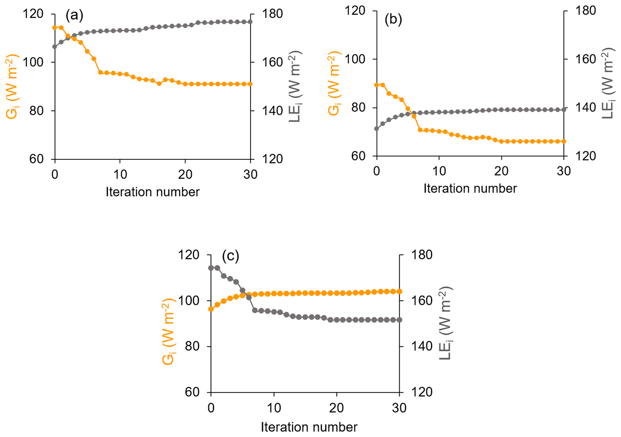
Figure 4Illustrative examples of iterative stabilization of STIC-TI Gi (yellow marker line) and LEi (grey marker line) in (a) IND-Jai, (b) AU-ASM, and (c) US-Ton.
The noteworthy features of STIC-TI are (1) estimating G by modifying the mechanistic MV2007-TI model using noon and midnight TS information from thermal remote sensing observations available through a polar-orbiting satellite platform (e.g., MODIS Aqua), (2) coupling the mechanistic MV2007-TI G model with STIC1.2 to simultaneously estimate surface moisture availability (M), G, and SEB fluxes, (3) introducing water stress information in G (through M) to better constrain the aerodynamic and canopy–surface conductances as well as the SEB fluxes, and (4) derivation of the amplitude of ecosystem-scale surface soil temperature (from the topsoil to 0.1 m soil depth).
3.1.3 Generation of remote sensing inputs
Two of the key variables in SEB modeling are TS and εs. These two variables were retrieved at 923 m spatial resolution from MODIS Aqua noon–night TIR observations (MYD11A2) in bands 11.03 and 12.02 µm using a generalized split-window algorithm (Wan and Li, 1997). For optimal retrieval, tractable sub-ranges of atmospheric column water vapor and lower-boundary air surface temperature were used. Land surface emissivity was estimated from land cover types and anisotropy factors. The MYD21A2 LST product was generated using the temperature–emissivity separation (TES) algorithm (Hulley et al., 2016) and an improved water vapor scaling method to remove the atmospheric effects. Albedo was estimated from the MODIS (MCD43A2 Version 6.0) Bidirectional Reflectance Distribution Function and Albedo (BRDF/Albedo) daily dataset (Schaaf et al., 2002) at 462 m spatial resolution. Actual albedo is a value which is interpolated between white-sky and black-sky albedo as a function of fractional diffuse skylight (which is a function of aerosol optical depth). NDVI was obtained from the level-3 MODIS vegetation index product (MYD13Q1, version 6.1), which is generated every 16 d at 250 m (m) spatial resolution. All the input remote sensing variables mentioned in Table 2 were resampled to the spatial resolution of the MYD11A2 product (923 m).
3.2 Sensitivity and statistical analysis
The accuracy of STIC-TI heavily depends on the accuracy of TS, NDVI, and αR due to the dual role of TS in estimating M and Gi, the role of NDVI in Gi, and the combined role of TS and αR in estimating RNi. Therefore, one-dimensional sensitivity analysis was conducted to assess the impacts of uncertainty in TS, NDVI and αR on Gi, Hi and LEi. The sensitivity was assessed by varying noontime TS by ±0.5, ±1.0, and ±1.5 K (keeping nighttime TS constant so that amplitude can vary automatically), varying NDVI by ±0.05, ±0.10, and ±0.15, and varying albedo by ±0.02, ±0.05, and ±0.10, respectively. SEB fluxes were computed by using TS, NDVI, and αR for three different periods of the year in all eight ecosystems. Sensitivity analyses were conducted by increasing and decreasing systematically TS, NDVI, and αR from its central value while keeping the other variables and parameters constant. This procedure was selected because the fluxes and intermediate outputs of the STIC-TI model reflect an integrated effect due to uncertainty in TS. In the first run, SEB fluxes were computed using in situ TS measurements obtained from the flux tower outgoing longwave radiation measurements. Then TS was increased and decreased at a constant interval and a new set of fluxes was estimated. In the similar way, αR and NDVI were increased and decreased at constant intervals, and a new set of fluxes was computed. The sensitivity of STIC-TI was assessed by Eq. (14).
Ei0 is the estimated (original) model output, and EiM is the estimated (modified) output obtained by changing the variable whose sensitivity is to be tested. Oi is the actual measurements. Apart from the sensitivity analysis, the following set of statistical metrics was used to assess model performances.
R2 is the coefficient of determination, RMSE is the root-mean-square error, BIAS is the mean bias, MAPD is the mean absolute percent deviation, KGE is the Kling–Gupta efficiency, n is the total number of data pairs, and the bar indicates the mean value of the measured variable and the model estimates of the same variable. Ei and Oi are the model-estimated and model-measured SEB fluxes, r is the Pearson correlation coefficient, is the average of the measured values, is the average of the estimated values, σo is the standard deviation of observation values, and σE is the standard deviation of the estimated values. The KGE has been widely used for calibration and evaluation of hydrological models in recent years, and it combines the three components of the Nash–Sutcliffe efficiency (NSE) of model errors (i.e., correlation, bias, ratio of variances or coefficients of variation) in a more balanced way, but it has not been widely used for analyzing the ET model performances. KGE = 1 indicates perfect agreement between modeled estimates and observations. The performance of a model is considered “poor” for KGE between 0 and 0.5, and models with negative KGE values are considered “not satisfactory”.
4.1 Ecosystem-scale surface soil temperature amplitude (A)
The scaling functions developed to estimate ecosystem-scale (1 km) surface soil temperature amplitude (A) from point-scale TSTA were used to estimate Gi. However, before the development of the scaling functions, analysis was carried out to investigate the relationship of soil temperature amplitude between the two different spatial scales. The scatterplot (Fig. 5a) of the noon–night LST difference (ΔTs) versus TSTA for different albedo classes showed a linear increase in ΔTs with increasing TSTA. However, some divergence of data points within the cluster was also noticed, which could be associated with different albedo (αR) levels. A bivariate linear function was fitted between TSTA as a predictand (Y) versus ΔTs (Tsd−Tsn) and αR as predictors (X1 and X2, respectively). The function was found to be by combining the data of nine ecosystems (r=0.86). The coefficients in the above expressions correspond to B1 (0.59), B2 (51.3), and B3 (8.66) of Eq. (5). The estimated amplitude from these ecosystem-scale predictors and scaling functions was treated as an ecosystem-scale surface soil temperature amplitude (A).
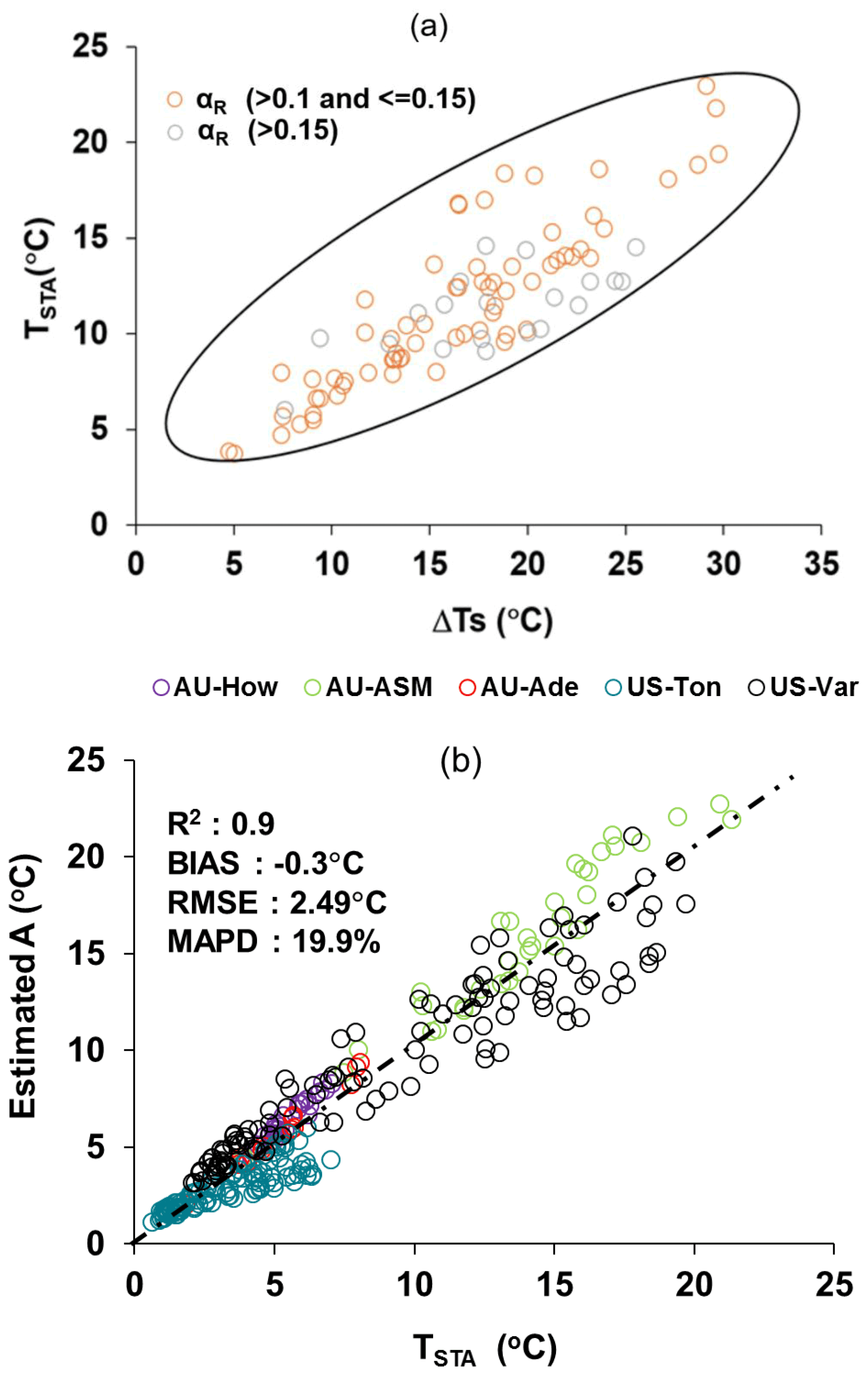
Figure 5(a) Two-dimensional scatterplots between (ΔTs) versus TSTA at different αR levels over different ecosystems. Here TSTA on the y axis is the observed soil temperature amplitude that is used to develop the scaling function, and ΔTs is the noon–night LST difference of MODIS AQUA. (b) Validation of ecosystem-scale estimates of A from the above functions over different sites.
Validation of ecosystem-scale estimates of A from the above functions over different sites is shown in Fig. 5b with respect to TSTA for the independent datasets. The estimated A was found to have an MAPD of 19.9 %, negative bias, and R2=0.90 over different ecosystems. The temporal variation of estimated A and TSTA is shown in Fig. D1 in Appendix D. Further analysis was carried out to investigate the bias in A at three fractional vegetation cover (fc) classes (fc<0.3; ; fc>0.5) representing bare soil (class 1), 30 %–50 % canopy cover (class 2), and more than 50 % canopy cover (class 3), respectively. While negative bias was noted for class 1 and class 3 (−0.54 and −0.83 ∘C), the bias was positive (0.49 ∘C) in the intermediate fc, which represents sparse and patchy canopy cover. The signals of surface albedo, emissivity, and temperature of soil surface and canopy are relatively pure in class 1 and class 3 as compared with class 2, where the surface signal carries more heterogeneity. Given that TSTA is computed from the in situ measurements, it is likely to carry more heterogeneity in class 2 as compared with the other two classes. The land surface emissivity in MYD11A2 was estimated from land cover types and the anisotropy factor, which have differential impacts on TST and TS, leading to such an opposite bias in class 2 as compared with class 1 and class 3.
4.2 Sensitivity analysis of STIC-TI Gi, LEi and Hi to land surface variables
4.2.1 Sensitivity of Gi to land surface variables
The average sensitivity of Gi to three land surface variables (TS, NDVI, αR) by combining the estimates of wet and dry periods is shown in Fig. 6. Gi was found to be substantially sensitive to TS, with error magnitude ranging from 2 % to 18 % due to TS uncertainties of ±0.5–2.5 K (Fig. 6a), with greater sensitivity to TS during the summer season. The median sensitivity of Gi due to ±5 %–10 % uncertainty in αR varied from 5 % to 12 % in all the ecosystems (Fig. 6b). The uncertainties in NDVI revealed 2 % to 15 % error in Gi estimates (Fig. 6c), and no significant difference in the mean sensitivity due to NDVI uncertainties was noted between the ecosystems. The sensitivity of Gi decreased with increasing values of NDVI.
4.2.2 Sensitivity of LEi and Hi to land surface variables
Both LEi and Hi were sensitive to TS on the order of 2 %–29 % (LEi) and 5 %–35 % (Hi) for a TS uncertainty of ±0.5–2.5 K from its mean values (Table 3). Interestingly, LEi was more sensitive to TS uncertainties as compared with Hi in the rainfed ecosystems. The highest mean sensitivity of LEi to TS was found in arid (IND-Jai: 2 %–28 %), semi-arid (AU-ASM: 5 %–21 %), tropical savanna (IND-Dha: 3 %–26 %), savanna (US-Ton: 4 %–29 %), and arid (US-Var: 3 %–26 %) ecosystems. The mean sensitivity of Hi to TS was maximum in sub-humid (IND-Sam: 2 %–32 %), semi-arid (IND-Naw: 2 %–28 %), and savanna (AU-Ade: 8 %–17 %) (Table 3). A greater sensitivity of the SEB fluxes due to αR uncertainties was found than due to NDVI. The median sensitivity of LEi and Hi due to 10 % uncertainty from mean αR varied within 2 %–16 % in all the ecosystems (Table 3). By contrast, errors in the two SEB fluxes were substantially low (2 %–13 %) due to ±0.05–0.15 uncertainty from mean NDVI (Table 3).
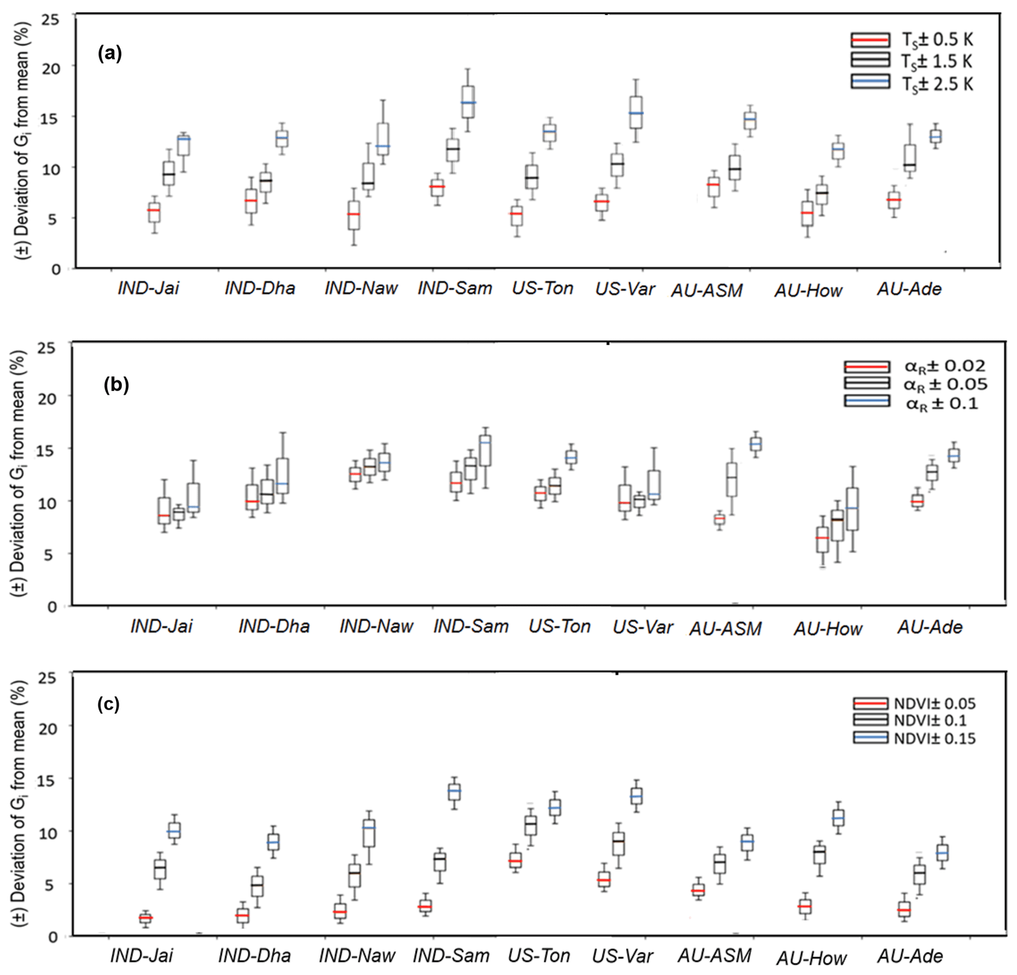
Figure 6Sensitivity of STIC-TI Gi due to uncertainties in TS (a), αR (b), and NDVI (c) for nine flux tower sites in India, the United States, and Australia. The uncertainties were introduced by taking the mean values of these variables during three different periods (summer, rainy, and winter) of a year. Mean uncertainties of the three periods are presented in the figure.
Table 3Sensitivity (in percent) of LEi and Hi due to TS, NDVI, and αR uncertainties.

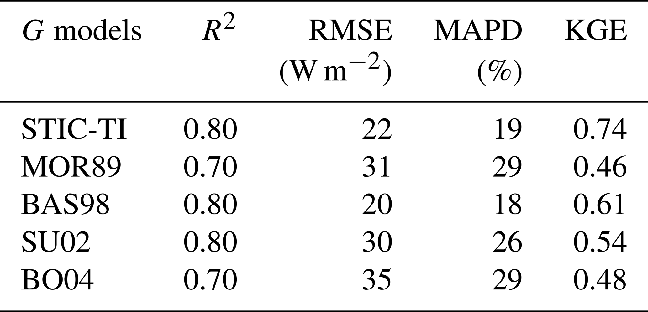
4.3 Comparative evaluation of the STIC-TI and contemporary Gi models
The performances of the STIC-TI and existing Gi models were evaluated and compared with respect to in situ Gi measurements. The existing models reported by Moran et al. (1989), Bastiaanssen et al. (1998), Su (2002), and Boegh et al. (2004) have been considered for comparing with the TI-based model. These four existing models are referred to here as MOR89, BAS98, SU02, and BO04, respectively. While the models MOR89, SU02, and BO04 are based on linear regression between G versus NDVI, BAS98 is based on multivariate regression of G with NDVI, LST, and αR. The performance of the STIC-TI was substantially better as compared with MOR89, SU02, and BO04 with respect to MAPD (19 %), RMSE (22 W m−2), and the coefficient of determination (R2=0.8) when compared with in situ measurements over one Indian, three Australian and two US flux tower sites (Table 4) and comparable with the BAS98 Gi model. The validation plot of retrieved noontime Gi from STIC-TI is shown in Fig. 7.
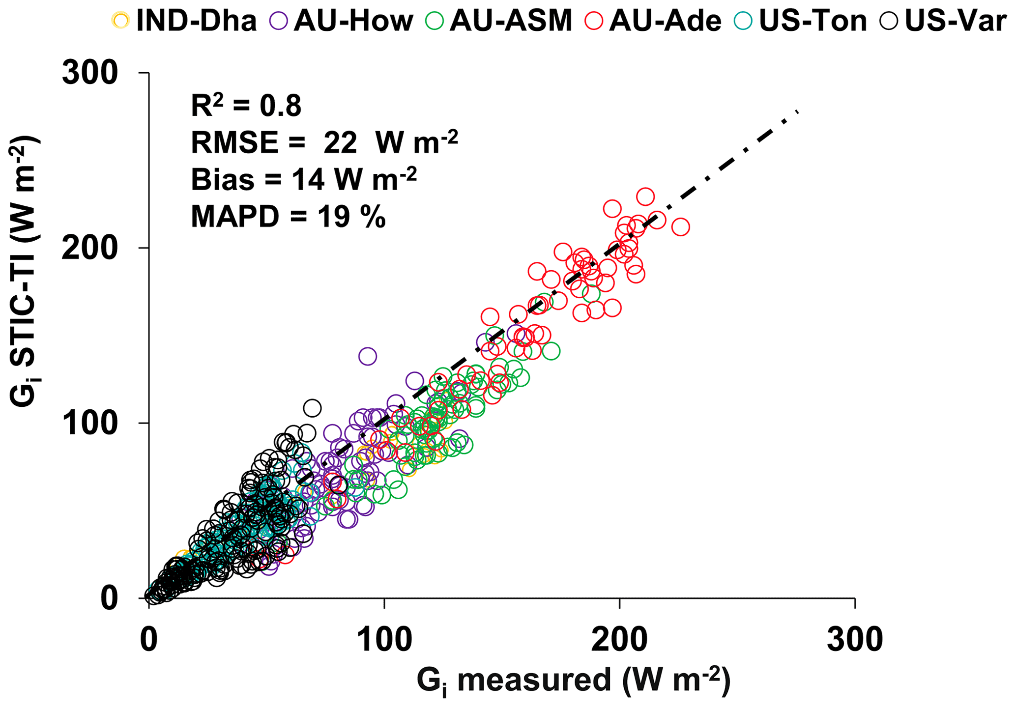
Figure 7Validation of noontime (13:30) Gi estimates with respect to in situ measurements in different ecosystems. The regression between the two sources of Gi is Gi (STIC-TI) = 0.90 Gi (tower) −0.10.
Table 4A comparison of error statistics of Gi estimates from STIC-TI and existing Gi models over different ecosystems.
The RMSE varied from 9 to 20 W m−2, with MAPD ranging from 12 % to 21 % across individual flux tower sites. A high magnitude of Gi was predicted in the arid and semi-arid systems (120–240 W m−2) as compared with the humid systems (20–90 W m−2), which was in close correspondence to the observations. The model also captured the range of Gi that is generally found in different biomes (20–140 W m−2 for grasslands, 20–90 W m−2 for cropland) (Purdy et al., 2016). Due to the paucity of Gi measurements, direct validation of Gi was only possible for 32 d (concurrent to MODIS overpass) at the IND-Dha site. Overall, STIC-TI tends to provide reasonable G estimates for the terrestrial ecosystems, with a soil temperature amplitude above 5 ∘C.
4.4 Evaluation of STIC-TI LEi, Hi, and EF
The modeled versus measured LEi and Hi showed good agreement in all nine ecosystems with RMSE in LEi and Hi estimates using the MYD11 LST product on the order of 29–62 W m−2 and 26–61 W m−2, MAPD of 9 %–31 % and 20 %–36 %, BIAS of −29 to 38 W m−2 and −44 to 32 W m−2 (Fig. 8a, b; Table 5), and a high R2 of 0.8.
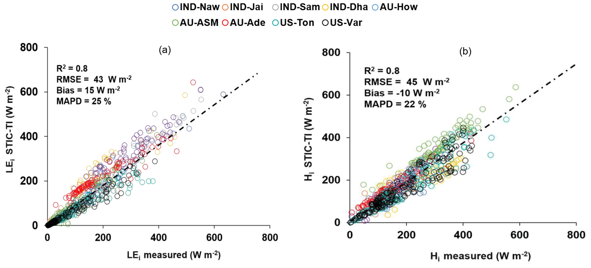
Figure 8(a) Validation of STIC-TI LEi estimates with respect to in situ measurements in different ecosystems. (b) Validation of STIC-TI Hi estimates with respect to in situ measurements in different ecosystems.
Table 5Error statistics of STIC-TI LEi and Hi estimates with respect to EC measurements in different ecosystems of India, the USA, and Australia using the MYD11A2 LST product for all nine sites and using the MYD21A2 LST product for three semi-arid and arid sites. The statistics obtained by using MYD21A2 LST are shown in the parentheses.
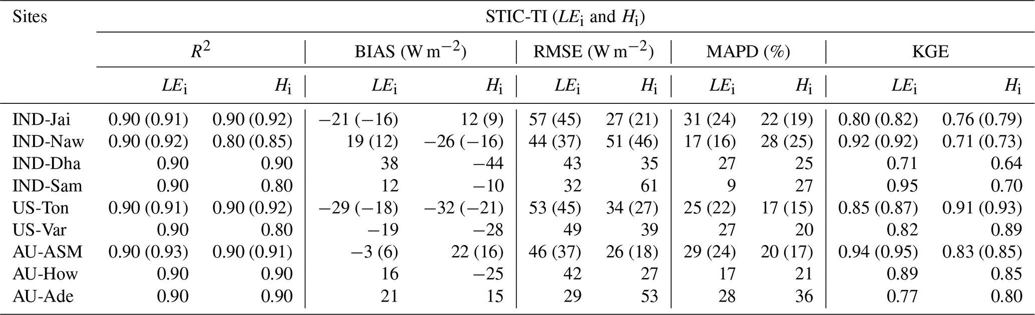
Arid ecosystems in India (IND-Jai) and the US (Ton and Var) and the semi-arid ecosystem in Australia (AU-ASM) revealed relatively high MAPD (31 %, 25 %, 27 %, and 28 %) (Table 5). In general, STIC-TI was able to produce the dominant convective heat fluxes with respect to the EC measurements, as evident through the low RMSE for Hi and high RMSE for LEi in IND-Jai, US-Ton, US-Var, and AU-Ade, where LEi is inherently low except for a few rainy days. A uniform distribution of data points around the 1 : 1 validation line (Fig. 8a) indicated an overall low BIAS in LEi estimates. However, modeled Hi was consistently lower than the observations (negative BIAS) in the tropical savanna (IND-Dha and AU-How) and semi-arid (IND-Naw) ecosystems (−44)–(−25) and −26 W m−2), while a consistent positive BIAS was observed in AU-ASM (semi-arid), AU-Ade (savanna), and US-Var (arid) (Fig. 8b; Table 5). This consequently led to an overall low negative BIAS (−10 W m−2) and a relatively low R2 in Hi (R2=0.8) as compared with the errors in LEi (BIAS = 15 W m−2, R2=0.9). The regression between the modeled and tower measurements of LEi is LEi (STIC-TI) = 0.98LEi (tower) − 0.266. The regression between the modeled and tower measurements of Hi is Hi (STIC-TI) = 0.93Hi (tower) + 4.90. The KGE statistics varied in the range of 0.71–0.95 for LEi and in the range of 0.64–0.91 for Hi, respectively, across all nine flux tower sites, thus revealing a reasonably high efficiency of the model in capturing the magnitude and variability of SEB fluxes.
The impact of the MODIS Aqua day–night view angle difference (δVZA) on STIC-TI fluxes was investigated. Estimated errors in terms of the mean percent deviation in LEi, Hi, and Gi with respect to measurements for each 10∘ bin over 16 angular bins within ±80∘ were analyzed in response to the mean δVZA of each angular bin. Gi errors (X) were found to be significantly correlated with δVZA (Y) in a parabolic (; r=0.73) pattern (refer to Appendix F, Fig. F1a). Errors in Gi on the order of −5 % to 10 %, 10 %–15 %, and > 15 % were largely found to be within ±30, ±45, and >45 to −80∘ δVZA, respectively. The errors in Hi were found to have a strong linear (, r=0.77) dependence on δVZA (refer to Appendix F, Fig. F1b). However, a weak dependence of LEi errors (, r=0.5) on δVZA (refer to Appendix F, Fig. F1c) was found, as the majority of the errors were within ±10 %, which corresponded to ±60∘ δVZA. The nature of the relations and the degree of dependency of the model flux errors on δVZA in this study would be helpful for minimizing the error budget in surface energy balance fluxes from future thermal infrared missions with day–night observations.
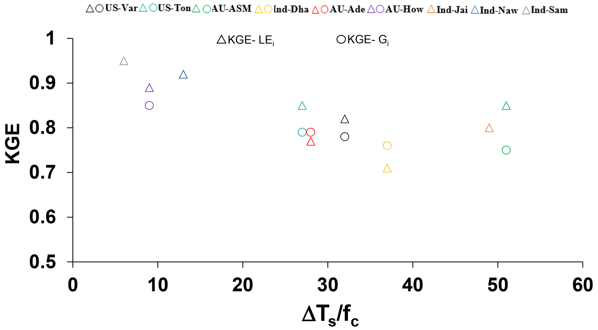
Figure 9Relationship between the KGE of STIC-TI (Gi and LEi) with in different terrestrial ecosystems.
Further investigation was done on whether the KGE for STIC-TI Gi and LEi follows any systematic pattern, and the ratios ΔTS and fc were used as a proxy for surface heterogeneity and dryness. The plot of the KGE of Gi and LEi with this ratio is shown in Fig. 9. KGE–Gi was found to show a systematic decrease with an increase in the ΔTS–fc ratio of up to 40, after which it remained unchanged with an increase in the ratio. Although the KGE of LEi also decreased (20 % reduction) with an increase in the ΔTs–fc ratio, KGE-LEi was found to increase beyond ΔTs−fc 40. This revealed that the model efficiency remained high (>0.8) within certain dryness limits (ΔTs−fc ratio <20 and >50) and that the efficiency reduced moderately (within 0.7–0.8) for intermediate dryness. Interestingly, the use of MYD21A2 LST in STIC-TI showed improvements (see the parentheses in the different columns in Table 5) in LEi and Hi error statistics as compared with using MYD11A2 LST in terms of higher R2 and KGE and lower RMSE in LEi (3 %–8 % less) and Hi (2 %–3 % less) for semi-arid and arid sites such as IND-Jai, IND-Naw, and US-Ton.
An independent evaluation of multi-temporal heat fluxes over two US flux sites for the years 2016–2018 is shown in Figs. 10 and 11. STIC-TI Gi estimates with the MYD11A2 LST product showed a close match with in situ measurements with respect to intra- and inter-annual variability in Gi, followed by LEi and Hi. This further demonstrates the merit of the coupled model for reproducing ecosystem-scale Gi estimates, especially for shorter and open canopies.

Figure 10Illustrative examples of the temporal evolution of STIC-TI-derived fluxes using the MYD11A2 LST product versus observed SEB fluxes for 3 consecutive years from 2016 to 2018 in a grassland ecosystem in the United States (e.g., US-Var).
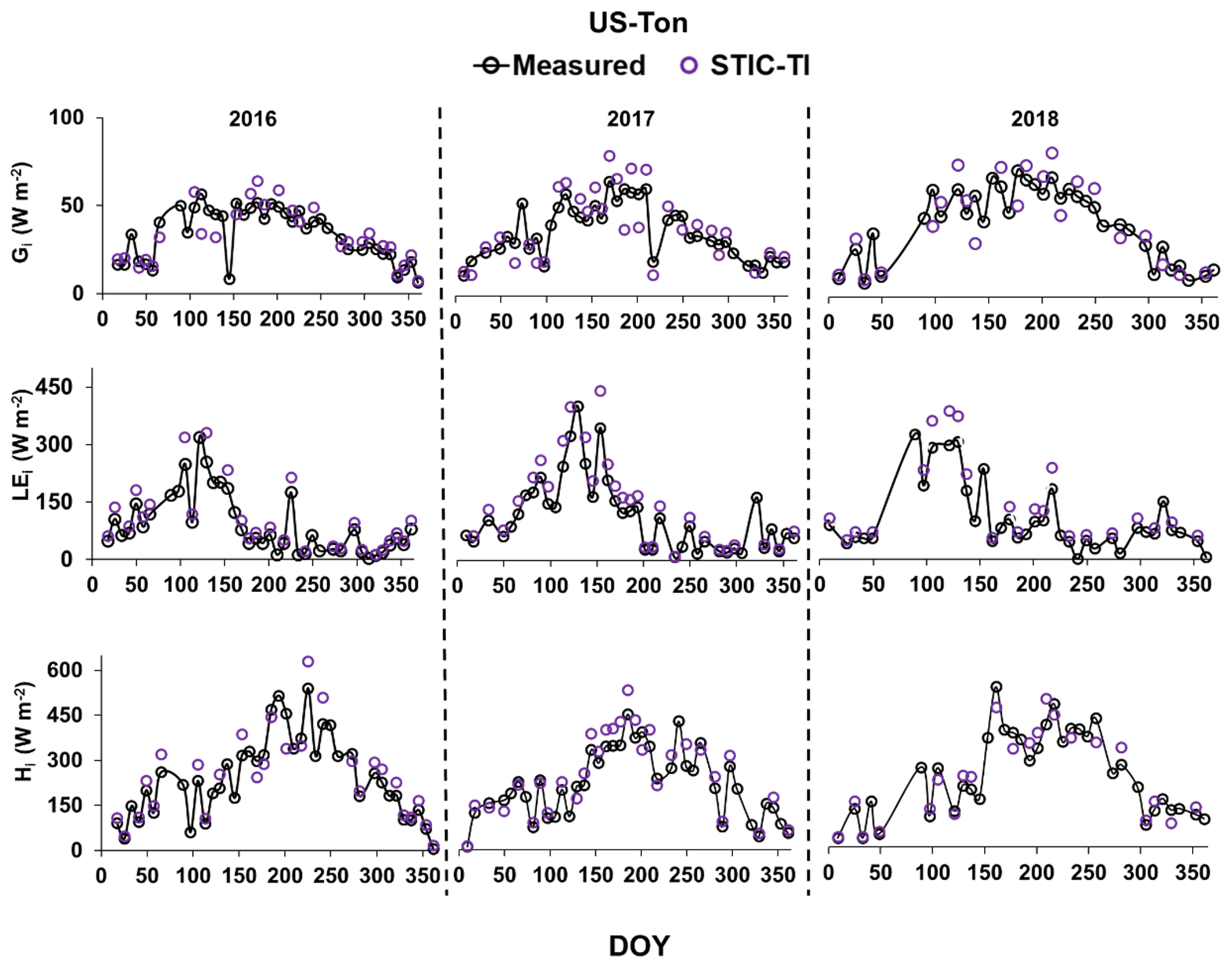
Figure 11Illustrative examples of the temporal evolution of STIC-TI-derived fluxes using the MYD11A2 LST product versus observed SEB fluxes for 3 consecutive years from 2016 to 2018 in a woody savanna ecosystem in the United States (e.g., US-Ton).
The temporal behavior of STIC-TI and the observed evaporative fraction (EF) (ratio of LE and RN–G) (Fig. 12) along with observed monthly rainfall (P) distinctly captured the substantial temporal variability in EF during the dry-to-wet transition in the Indian study sites, which also corresponded to low (high) θ and P. In IND-Naw and IND-Sam, a marked rise (>0.4) in STIC-TI EF was noted during days of the year (DOYs) 25 to 75, when wheat is grown under assured irrigation. The impact of irrigation is thus captured by the substantial increase in EF in the absence of P. In contrast, the rainfed grassland system (IND-Jai) showed a peak EF (∼ 0.8), which corresponded to southwestern monsoon rainfall during June to September and a progressive decline in EF during the dry-down period in October to April corresponding to the post southwestern monsoon phase. Some intermittent spikes in EF were also noted during the dry-down phase in both STIC-TI and observations. The intermittent EF spikes during the soil moisture dry-down phase could be due to enhanced LE through moisture advection from the surrounding vegetation causing a greater enhancement of evaporation than expected. This is known as the “clothesline effect”, which frequently occurs in semi-arid and arid ecosystems. In addition to IND-Jai, the response of both modeled and measured EF to wet and dry spells was also noted during the southwestern monsoon period at all other flux tower sites of India.
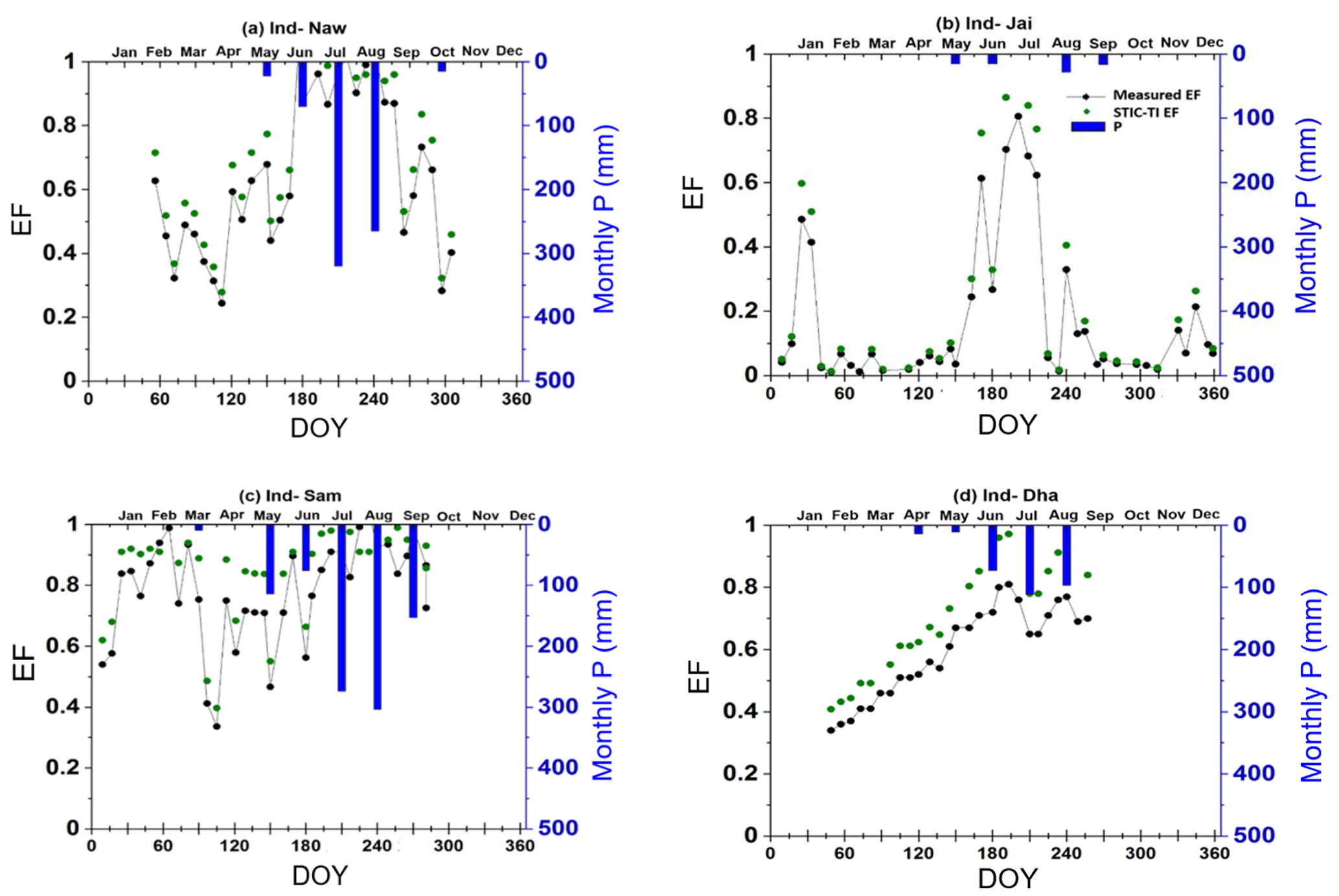
Figure 12Illustrative examples of the temporal variation of STIC-TI-derived EF using the MYD11A2 LST product with respect to measured EF and P in (a) IND-Naw, (b) IND-Jai, (c) IND-Sam, and (d) IND-Dha.
The temporal behavior of EF from the STIC-TI using the MYD11A2 LST product and EC measurements along with measured θ and P at the OzFlux and AmeriFlux sites also revealed (Fig. 13) a close correspondence of STIC-TI to EC observations. Low EF (0.05–0.40) during the dry season around DOY 100–250 and high EF (>0.4) during the wet season (DOY 1–120 and 300–360) in AU-ASM, US-Ton, and US-Var was observed. The analysis showed that STIC-TI EF can capture the annual variability of observed EF and its responses across different ecosystems during the wet and dry seasons. The plots of STIC-TI EF versus measured θ (in the inset of Fig. 13) revealed triangular scatter close to the right-angled triangle with a positive slope of the hypotenuse in three ecosystems: AU-ASM, US-Var, and US-Ton. This showed, in the water-controlled ecosystems, that distinct wet–dry seasons exist and that the positive EF–θ relationship is an outcome of the soil moisture controls on transpiration during the dry season.
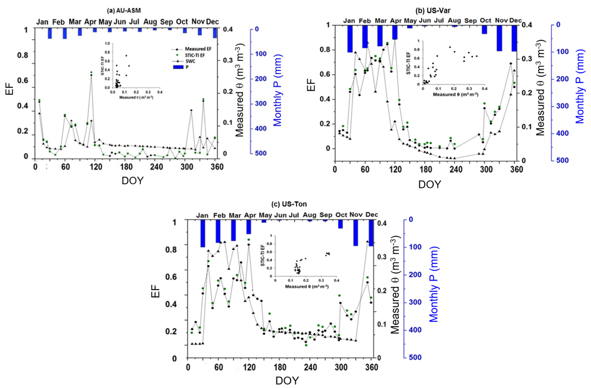
Figure 13Comparison of the temporal variation of STIC-TI-derived EF using the MYD11A2 LST with respect to measured EF, θ, and P in (a) AU-ASM, (b) US-Var, and (c) US-Ton. The scatterplots in the inset show the relationship between STIC-TI EF with respect to measured θ.
5.1 Interaction of flux and internal SEB metrices
From Sect. 4.1 we found a relatively reduced sensitivity of Gi to TS uncertainties. In any given condition, if an over(under)estimation of M due to noontime TS uncertainties (through Eq. 13) leads to an over(under)estimation of Γ, the effects of such over(under)estimation of Γ (due to noontime TS uncertainties) tend to be compensated by under(over)estimation of amplitude A (in Eq. 5), ultimately leading to a reduction in the sensitivity of Gi to TS. While the scatter between G versus A for a wide range of Γ (Fig. 14a) revealed large scatter with increasing amplitude under the dry conditions (low Γ), the scatter between Γ versus TS for different M (Fig. 14b) revealed an exponential reduction in Γ with increasing TS and dryness and almost no significant change in Γ with increasing TS at a constantly high dryness (M<0.25). Thus, the confounding effects of Γ, A, and M through Eqs. (3), (5), (12), and (13) led to a reduction in sensitivity of G to TS, as exemplified in Fig. 14.
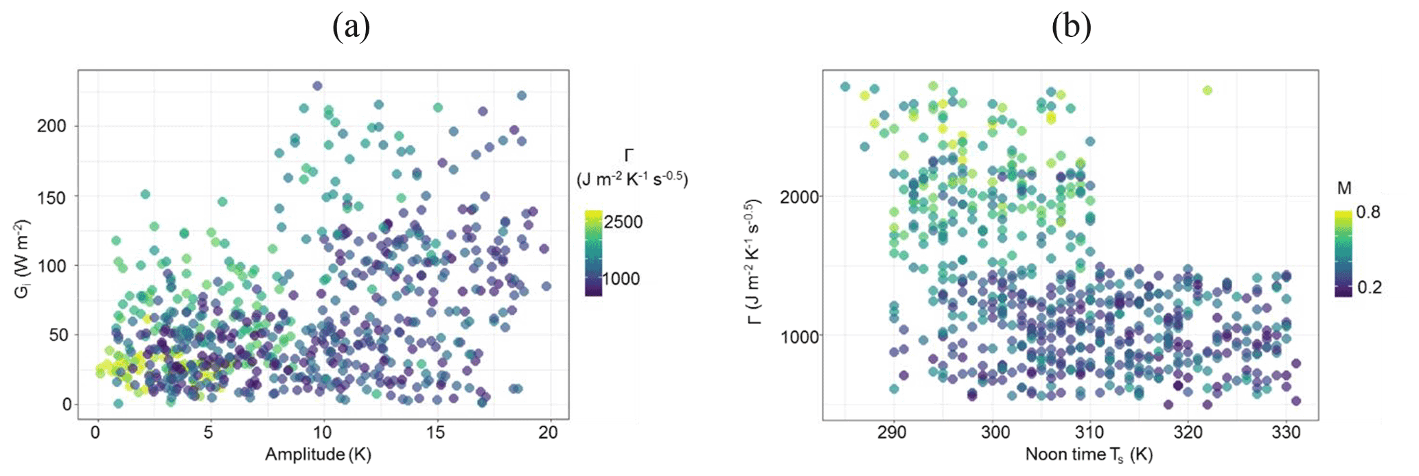
Figure 14Response plots among parameters of the TI-based Gi model, such as (a) Gi versus amplitude (A) for varying Γ and (b) noontime TS versus Γ with varying M.
Concerning LEi and Hi, dual uncertainties could be propagated in both the fluxes through daytime TS (through M and Gi), leading to high sensitivity of these two SEB fluxes due to TS perturbations. The relatively high sensitivity of LEi to TS (as compared with Hi) in the non-irrigated ecosystems could be due to partial compensation of in both the numerator and denominator of the PMEB equation for H (Eq. C7 of Appendix C). A recent study (Fig. 10 in Mallick et al., 2018a) showed high sensitivity of gS due to TS (a 1 % change in TS led to a 5.2 %–7.5 % change in gS) as compared with gA sensitivity to TS (a 1 % change in TS led to a 1.6 %–2 % change in gA), suggesting that errors in gS due to TS uncertainty tend to be larger than errors in gA. Partial cancellation of the conductance errors in the numerator of Eq. (C7) might have resulted in compensation of Hi errors in the water-limited ecosystems. In this environment, the variability of LEi is mainly dominated by , which makes LEi highly sensitive due to TS uncertainties. Combined uncertainty due to in the denominator and gA in the numerator of Eq. (C6) resulted in greater sensitivity in LEi to TS in the arid and tropical savanna ecosystems (Mallick et al., 2015, 2018a; Winter and Eltahir, 2010). The very low sensitivity of LEi and Hi due to uncertainties in NDVI is because NDVI was not used in the conductance parameterizations and effects due to NDVI in STIC-TI only being propagated through Gi. The sensitivity of LEi and Hi to albedo was mainly due to the dependence of net radiation (RNi) on albedo, and any resultant uncertainty in RNi (due to albedo) tends to be reflected in the sensitivity of LEi and Hi to albedo.
5.2 Possible sources of errors in SEB flux evaluation
In STIC-TI, underestimation and overestimation errors in Gi in different ecosystems (Fig. 7) could originate due to the errors in the MYD11A2 LST product. A host of studies previously reported that the standard deviations of errors in retrieved emissivity in bands 31 and 32 are 0.009, and the maximum error in retrieved TS of the MOD11A1 LST falls within 2–3 K, which is mainly due to the errors in surface emissivity correction (Duan et al., 2017; Wan, 2014). In the present analysis, we found an overestimation error of MODIS TS in the range of 0.5–1.5 K when compared with in situ infrared temperature measurements at the tropical savanna site. As mentioned in Sect. 3.1, a positive (negative) bias in TS would tend to an overestimation (underestimation) of amplitude (A) in Eq. (5), underestimation (overestimation) of M in Eq. (13), and consequent underestimation (overestimation) of Γ (Eq. 12) and Gi, respectively. Furthermore, the standard deviation of NDVI surrounding the tower sites varied from 0.01 to 0.05 when compared with the ground measurements, which could be another source of error in the STIC-TI model. In addition, NDVI saturates at LAI > 3. However, STIC-TI provides direct estimates of ecosystem G and is independent of RN.
Despite the comparable accuracy of current G estimates with the G model of Bastiaanssen et al. (1998), the foundation of STIC-TI lies in the use of soil moisture characteristics with varying soil textural types which are known to influence the soil heat conductance and thereby G. Thus, the control of soil moisture on evaporation is explicitly included in STIC-TI as opposed to the semi-empirical G function of Bastiaanssen et al. (1998). The higher accuracies of the TI-based thermal diffusion model as compared with RN-based empirical G models were also reported by Purdy et al. (2016) at daily or longer timescales in cropland and grassland. All these G model estimates may at times differ from in situ measurements due to not accounting for leaf litter presence or the layer on the soil floor in the remote-sensing-based G model.
The overestimation (underestimation) of LEi (Hi) is also due to the effects of the spatial resolutions of different input variables on these two SEB fluxes and conducted statistical evaluation with respect to the measured SEB fluxes. Eswar et al. (2017) demonstrated the need for spatial disaggregation models for monitoring LEi at field scale using contextual models by disaggregation of the evaporative fraction (Λ) and downwelling shortwave radiation ratio (RG). Using different disaggregation models, they estimated LEi at 250 m spatial resolution and reported an RMSE of 30–32 W m−2 as compared with LEi obtained at a 1000 m spatial resolution with an RMSE of 40–70 W m−2 over different sites in India. Anderson et al. (2007) reviewed different validation experiments conducted in diverse agricultural landscapes (Anderson et al., 2004, 2005; Norman et al., 2003) and reported RMSE in LEi in the range of 35–40 W m−2 (15 %) at 30–120 m disaggregated spatial resolution. Current analysis also brought out the need for noon–night thermal imaging with a spatial resolution finer than 1000 m to adequately capture the magnitude and variability of LEi in the terrestrial ecosystems, especially agroecosystems where average field sizes are lower (<0.5 ha) and fragmented, such as in India and other sub-continents.
As seen in Fig. 8a and Table 5, there is a gross overestimation of LEi with respect to the tower observations when MYD11A2 LST is used. The consistent positive BIAS in STIC-TI LEi in five out of nine sites is presumably due to the overestimation of RNi (Fig. B1 of Appendix B) and the underestimation of Gi. Figure 7 shows an overestimation of Gi for three OzFlux sites and US sites and an underestimation of Gi for the Indian site with Gi (STIC-TI) = 0.90 Gi (tower) − 0.10 and an overestimation of RNi at the ecosystem scale, with RNi (STIC-TI) = 0.78RNi (tower) + 58.92 (Appendix B2). This means that a systematic overestimation of net available energy (RNi−Gi) will be obvious in cases where STIC-TI shows an underestimation of Gi. Since available energy is an important component for estimating LE through the PMEB equation, an overestimation of net available energy leads to an overestimation of LE by STIC-TI. Sensible heat flux will be consequently underestimated due to the complementary nature of the PMEB equation. It may also be noted that the use of MYD21A2 LST led to a relatively better accuracy in LEi (3 %–8 %) and Hi (2 %–3 %) as compared with using MYD11A2 LST in semi-arid and arid ecosystems. The higher retrieval accuracy of MYD21A2 LST using the TES algorithm over MYD11A2 LST that uses a split-window algorithm (Wan and Li, 1997) is the main reason for obtaining higher accuracy in LEi and Hi estimates.
The standard deviations of the MODIS Aqua day–night overpass time over the study sites were found to be within 30–45 min (Sharifnezhadazizi et al., 2019), and the expected deviation in LST from the mean local time would be around ±0.75 K (Sharifnezhadazizi et al., 2019). Sensitivity analysis showed that resultant uncertainties in STIC-TI heat flux estimates would be on the order of ±5 %–7 % due to this LST uncertainty.
5.3 Effects of SEB closure
Given that there is a widespread lack of SEB closure () or residual energy balance, knowledge of the impact of different vegetation types and climatic variables on SEB “non-closure” is essential. A recent study by Dare-Idowu et al. (2021) covering eight growing seasons and three crops (maize, wheat, and rapeseed) in two sites of southwestern France showed that the systematic effect of each site on SEB closure was stronger than the influence of crop type and stage. The same study revealed a greater percentage of SEB closure under unstable atmospheric conditions and in the prevailing wind directions, and sensible heat advection accounted for more than half of the imbalance at both the sites.
In our study, using unclosed SEB observations for Indian sites in the absence of in situ Gi observations also added to the consistent positive BIAS in the statistical evaluation of LEi. A ubiquitous lack of energy balance closure on the order of 10 %–20 % worldwide at most of the EC sites is reported in different literatures (Stoy et al., 2013; Wilson et al., 2002), which implies a systematic underestimation (overestimation) of LEi (EC tower) (and/or the Hi EC tower). Accommodating an average 15 % imbalance in LEi (EC tower) would tend to diminish the positive BIAS in STIC-TI. Therefore, the pooled gain (0.98) and positive BIAS between the STIC-TI and tower LEi are determined by the overestimation of (RNi−Gi) combined with the underestimation of measured LEi from the EC towers. An underestimation of Hi (negative BIAS) is associated with two reasons: (a) ignoring the two-side aerodynamic conductance of the leaves (Jarvis and McNaughton, 1986; Monteith and Unsworth, 2013; Schymanski et al., 2017), which could lead to substantial underestimation of Hi, and (b) the complementary nature of the PMEB equation; if LEi is overestimated, Hi will be underestimated. In addition, frequent micro-advection fluxes alter measured in situ H and LE fluxes, but these advection conditions are not explicitly accounted for in the current STIC-TI model. At the EC tower sites, the fraction of the residual energy balance to RN can be quantified with respect to vegetation/crop growth characteristics or biophysical properties. However, where G observations are lacking, such as in many Indian EC tower sites, the TI-based G model can be used to fill up the missing G observations to quantify residual energy balance and to correct the SEB non-closure.
This study addressed one of the long-term uncertainties in thermal remote sensing of evaporation modeling in open-canopy heterogeneous ecosystems, which is associated with empirical methods of estimating ground heat flux. We demonstrated for the first time physical integration and coupling of a mechanistic ground heat flux model with an analytical evaporation model (Surface Temperature Initiated Closure, STIC) within the surface energy balance equation. The model is called STIC-TI, which uses satellite-based land surface temperature from MODIS Aqua and associated biophysical variables, and it has minimal independence of in situ measurements. The estimation of evaporation through STIC-TI does not require any empirical function for inferring the biophysical conductances. STIC-TI is independent of uncertain parameterizations of surface roughness and atmospheric stability and does not involve any look-up table for biome or plant functional attributes. By linking noon–night land surface temperature with a harmonics equation of thermal inertia and soil moisture availability, STIC-TI derived the ground heat flux and subsequently coupled it with evaporation. Independent validation of STIC-TI with respect to eddy covariance flux measurements from nine terrestrial ecosystems in arid, semi-arid, and sub-humid climates in India, the USA, and Australia led us to the following conclusions.
- i.
While the MODIS Aqua day–night view angle difference showed a strong impact on ground heat flux and sensible heat flux estimated deviations of STIC-TI (with respect to measurements), a relatively weak dependence of latent heat flux errors on the day–night view angle difference was noted.
- ii.
The most notable advantages of STIC-TI are firstly that it provides direct estimates of ground heat flux while simultaneously integrating the effects of soil water stress on ground heat flux and evaporation through the inclusion of noon–night land surface temperature information. Secondly, the ecosystem-scale surface soil temperature amplitude used in the ground heat flux model can advance our understanding of associated terrestrial ecosystem processes.
The requirement of few input variables in STIC-TI generates promise for surface–atmosphere exchange studies using readily available data from the current-generation remote sensing satellites (e.g., MODIS, VIIRS) that have noon–night land surface temperature observations. STIC-TI can also be potentially used for distributed ET mapping from future high spatial resolution (∼ 50–60 m) TIR missions with noon–night observations with high revisits, such as the Indo-French mission, TRISHNA (Thermal infrared Imaging Satellite for High-resolution Natural Resource Assessment) (Lagouarde et al., 2018, 2019), ESA's LSTM (Land Surface Temperature Monitoring), and NASA SBG (Surface Biology and Geology), respectively.
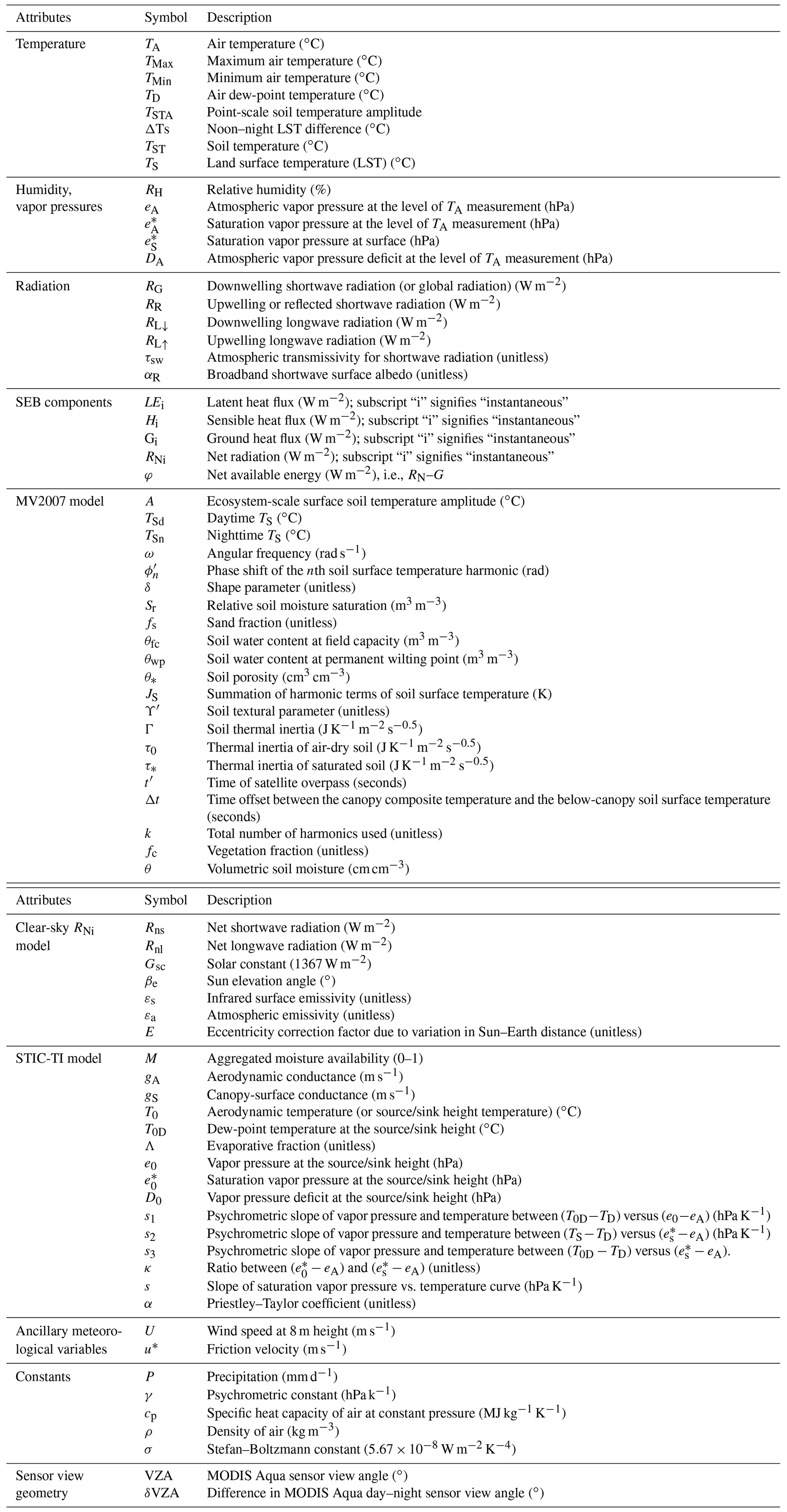
Table A2Summary of instruments used, height or depth and period of measurements, and measured variables at nine EC flux tower sites.
B1 Clear-sky instantaneous net radiation (RNi) model
Net radiation (RN) is defined as the difference between the incoming and outgoing radiation, which includes both longwave and shortwave radiation at the Earth's surface.
Terrestrial RN has four components: downwelling and upwelling shortwave radiation (RG and RR) and downwelling and upwelling longwave radiation (RL↓ and RL↑), respectively.
Out of these four terms mentioned in Eq. (B1), RG and RL↓ are dependent on various factors such as geographic location, season, cloudiness, aerosol loading, and atmospheric water vapor content and less on surface properties. On the other hand, the upwelling radiations in Eq. (B1) strongly depend on the surface properties such as surface reflectance and emittance, land surface temperature, and soil water content (Zerefos and Bais, 2013).
Instantaneous net radiation (RNi) can be derived using Eq. (B2) as follows (Mallick et al., 2007):
where Rns is net shortwave radiation (W m−2), Rnl is net longwave radiation (W m−2), and αR is the broadband surface albedo shortwave spectrum.
A WMO (World Meteorological Organization) shortwave radiation model (Cano et al., 1986) calibrated over Indian conditions (Mallick et al., 2007, 2009) was used to compute RG using the following equation:
where τsw is the global clear-sky transmissivity for the shortwave radiation (0.7), Gsc is the solar constant (1367 W m−2), ε is the eccentricity correction factor due to variation in the Sun–Earth distance, and βe is the Sun elevation in degrees.
RL↓ at any instance was calculated as follows:
where σ is the Stefan–Boltzmann constant ( W m−2 K−4), TA is the air temperature (∘C), and εa is the atmospheric emissivity.
Atmospheric emissivity (εa) was computed using the following equation (Bastiaanssen et al., 1998):
RL↑ at any particular instance was calculated as follows:
where εs is the surface emissivity in the thermal infrared (8–14 µm) spectrum and TS is the land surface temperature (∘C).
B2 Evaluation of STIC-TI RNi
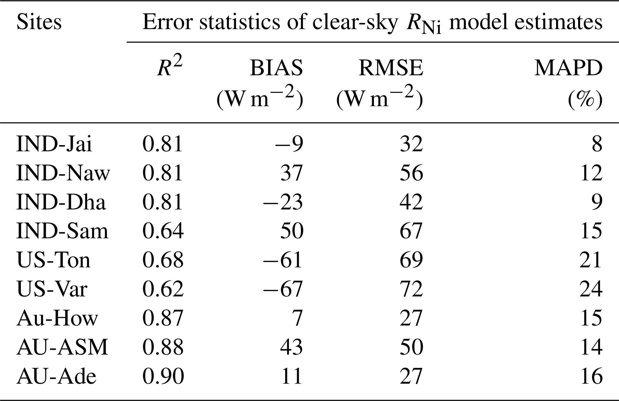
Comparison of the clear-sky RNi estimates with respect to in situ measurements revealed RMSE in RNi on the order of 27–72 W m−2, MAPD 8 %–24 %, BIAS (−67)–50 W m−2, and R2 varying from 0.62 to 0.90 across all the sites (Fig. B2, Table B2). Among the nine sites, a consistent underestimation of RNi was noted in IND-Dha, US-Ton, and US-Var (with BIAS of −23, −61, and −67 W m−2), whereas substantial overestimation of RNi was found in IND-Sam, IND-Naw, and AU-ASM with BIAS of 50, 37, and 43 W m−2, respectively (Table B2).
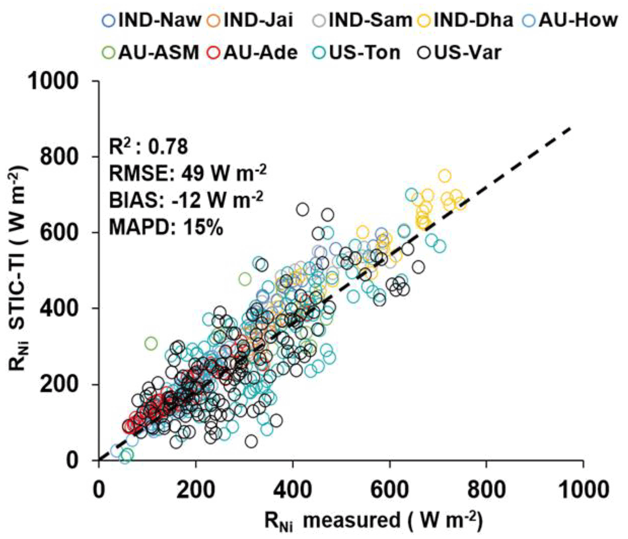
Figure B1Validation of STIC-TI-derived RNi estimates with respect to in situ measurements in different ecosystems. The regression equation between modeled versus in situ RNi is RNi (STIC-TI) = 0.78RNi (tower) + 58.92.
Table B1Performance evaluation statistics of clear-sky RNi estimates in nine different ecosystems.
C1 Estimating SEB fluxes using the STIC1.2 analytical model and thermal remote sensing data
STIC1.2 (Mallick et al., 2014, 2015a, b, 2016, 2018a) is a one-dimensional physically based SEB model and is based on the integration of satellite LST observations into the Penman–Monteith energy balance (PMEB) equation (Monteith, 1965). In STIC1.2, the vegetation–substrate complex is considered as a single unit. Therefore, the aerodynamic conductances from individual air–canopy and canopy–substrate components is regarded as an “effective” aerodynamic conductance (gA), and surface conductances from individual canopy (stomatal) and substrate complexes are regarded as an “effective” canopy–surface conductance (gS) which simultaneously regulates the exchanges of sensible and latent heat fluxes (H and LE) between the surface and atmosphere. One of the fundamental assumptions in STIC1.2 is the first-order dependence of these two critical conductances on M through TS. Such an assumption enabled an integration of satellite LST into the PMEB model (Mallick et al., 2016). The common expression for LE and H according to the PMEB equation is as follows.
In the above equations, the two biophysical conductances (gA and gS) are unknown, and the STIC1.2 methodology is based on finding analytical solutions for the two unknown conductances to directly estimate LE (Mallick et al., 2016, 2018a). The need for such analytical estimation of these conductances is motivated by the fact that gA and gS can neither be measured at the canopy nor at larger spatial scales, and there is no universally agreed appropriate model of gA and gS that currently exists (Matheny et al., 2014; van Dijk et al., 2015). By integrating TS with standard SEB theory and vegetation biophysical principles, STIC1.2 formulates multiple state equations in order to eliminate the need to use the empirical parameterizations of the gA and gS and also to bypass the scaling uncertainties of the leaf-scale conductance functions to represent the canopy-scale attributes. The state equations for the conductances are expressed as a function of those variables that are mostly available as remote sensing observations and weather forecasting models. In the state equations, a direct connection to TS is established by estimating M as a function of TS. The information of M is subsequently used in the state equations of conductances, aerodynamic variables (aerodynamic temperature, aerodynamic vapor pressure), and evaporative fraction, which is eventually propagated into their analytical solutions. M is a unitless quantity, which describes the relative wetness (or dryness) of a surface and also controls the transition from potential to actual evaporation, which implies M→1 under saturated surface conditions and M→0 under extremely dry conditions. Therefore, M is critical for providing a constraint against which the conductances are estimated. Since TS is extremely sensitive to the surface moisture variations, it is extensively used for estimating M in a physical retrieval scheme (detail in Appendix A3 of Bhattarai et al., 2018; Mallick et al., 2016, 2018a). It is hypothesized that linking M with the conductances will simultaneously integrate the information of TS into the PMEB model. To illustrate, we express the state equations by symbols, ; ; ; . Here, f, sv, v, and c denote the function, state variables, input variables (five input variables; radiative and meteorological), and constants (three constants), respectively. Here sv1 to sv4 are gA, gS, aerodynamic temperature (T0), evaporative fraction (Λ), and sv8 is M. Given the estimates of M, net radiative energy (RNi−Gi), TA, RH, the four state equations are solved simultaneously to derive analytical solutions for the four state variables and to produce a surface energy balance “closure” that is independent of empirical parameterizations for gA, gS, T0, and Λ. The state equations of STIC are given below.
Detailed derivations of these four state equations are given in Mallick et al. (2016, 2018a). However, the analytical solutions to the four state equations contain three accompanying unknowns; e0 (vapor pressure at the source/sink height), (saturation vapor pressure at the source/sink height), and Priestley–Taylor coefficient (α), and as a result there are four equations with seven unknowns. Consequently, an iterative solution was needed to determine the three unknown variables (as described in Appendix A2 in Mallick et al., 2016). Once the analytical solutions of gA and gS are obtained, both variables are returned into Eq. (13) to directly estimate LE.
In STIC-TI, an initial value of α was assigned as 1.26; initial estimates of were obtained from TS through temperature–saturation vapor pressure relationship, and initial estimates of e0 were obtained from M as, . Initial T0D and M were estimated according to Venturini et al. (2008) as described in Sect. 3.2, and initial estimation of G was performed from initial M using the equation sets Eqs. (2)–(11). With the initial estimates of these variables; first estimate of the conductances, T0, Λ, H, and LE were obtained. The process was then iterated by updating , D0, e0, T0D, M, and α (using Eqs. A9, A10, A11, A17, A16, and A15 in Mallick et al., 2016), with the first estimates of gS, gA, T0, and LE, and re-computing G, φ, gS, gA, T0, Λ, H, and LE in the subsequent iterations with the previous estimates of , e0, T0D, M, and α until the convergence of LE was achieved. Stable values of G, conductances, LE, H, T0, , e0, T0D, M, and α were obtained within ∼ 25 iterations. The inputs needed for computation of LEi (Eq. C6) are air temperature (TA), land surface temperature (TS), relative humidity (RH), net radiation (RNi) and soil heat flux (Gi).
The temporal variation of estimated A and TSTA is shown in Fig. D1. The annual variations of TSTA in different ecosystem was found to be within the ranges of 1–4 ∘C.
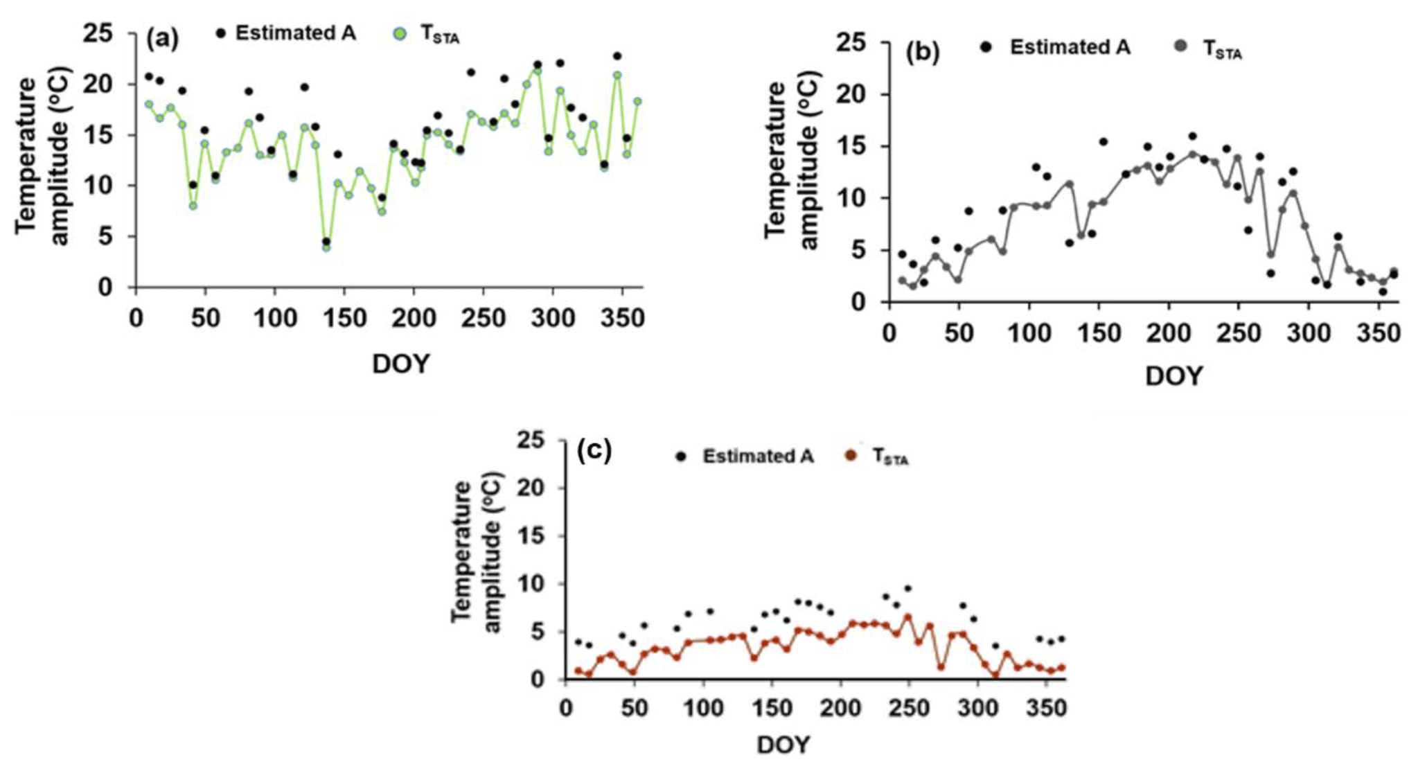
Figure D1Temporal variation of A and TSTA in (a) AU-ASM (2013), (b) US-Ton (2014), and (c) US-Var (2014).
Table E1Soil textural properties and their values used in the present study (Murray and Verhoef, 2007; Minasny and Hartemink, 2011; Anderson et al., 2007).
The day–night view angle effect on errors of STIC-TI heat flux estimates from measurements is shown in Fig. F1.
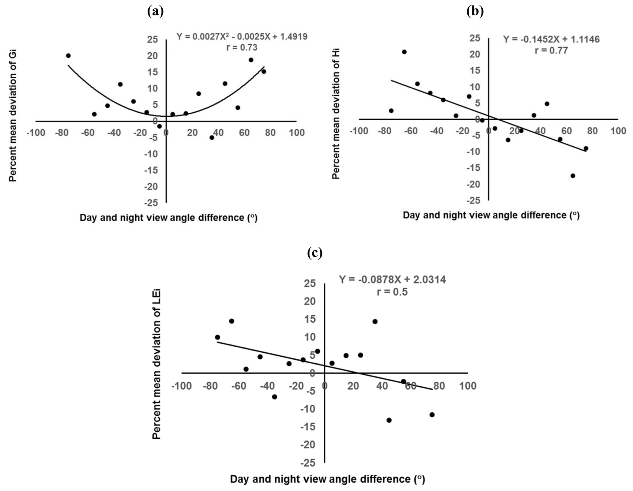
Figure F1Dependence of STIC-TI model flux error in terms of mean percent deviation from measurements of day–night view angle differences of MODIS Aqua expressed as a mean of the 10∘ bin for (a) Gi, (b) Hi, and (c) LEi.
Harmonized time series datasets over the study grids are available at https://doi.org/10.5281/zenodo.5806501 (Desai et al., 2022). The model code is available to the first author upon reasonable request.
KM and BKB conceptualized the idea. DD conducted STIC-TI model coding and simulations. BKB and DD conducted the data analysis in consultation with KM. DD and BKB wrote the first version of the manuscript, with KM writing the introduction, discussions, and conclusions. BKB and KM conducted all the analysis and writing during revision. All the authors contributed to discussions, editing, and corrections. BKB and KM jointly finalized the manuscript.
The contact author has declared that none of the authors has any competing interests.
Publisher's note: Copernicus Publications remains neutral with regard to jurisdictional claims in published maps and institutional affiliations.
The authors were supported by the Ministry of Earth Sciences (MoES), the government of India, and the National Environmental Research Council through the Indo-UK INCOMPASS program. Bimal K. Bhattacharya was supported by the deputy director of the EPSA and the director of SAC-ISRO for providing necessary support to participate in and contribute to the Indo-UK INCOMPASS program. Devansh Desai was supported by the Department of Physics, Electronics and Space Sciences, Gujarat University Ahmedabad, for providing the necessary support to carry out this work. Kaniska Mallick was supported through the International Mobility Fellowship of the Luxembourg National Research Fund (FNR). Kerry Cawse-Nicholson is supported by the Jet Propulsion Laboratory, California Institute of Technology, under contract with the National Aeronautics and Space Administration, and a government sponsorship is acknowledged. Dennis Baldocchi was supported by the NASA Ecostress project and the US Department of Energy, Office of Science, which supports the AmeriFlux project.
This research has been supported by the Fonds National de la Recherche Luxembourg (grant nos. INTER/MOBILITY/2020/14521920/MONASTIC and PRIDE15/10623093/HYDROCSI), the Natural Environment Research Council (grant nos. NE/L013819/1, NE/L013843/1, NE/L01386X/1, and NE/P003117/1), and the Office of Science (Ameriflux).
This paper was edited by Paul Stoy and reviewed by two anonymous referees.
Anderson, M., Norman, J., Mecikalski, J., Torn, R., Kustas, W., and Basara, J.: A Multiscale Remote Sensing Model for Disaggregating Regional Fluxes to Micrometeorological Scales, J. Hydrometeorol., 5, 343–363, https://doi.org/10.1175/1525-7541(2004)005<0343:AMRSMF>2.0.CO;2, 2004.
Anderson, M., Norman, J., Kustas, W., Li, F., Prueger, J., and Mecikalski, J.: Effects of Vegetation Clumping on Two–Source Model Estimates of Surface Energy Fluxes from an Agricultural Landscape during SMACEX, J. Hydrometeorol., 6, 892–909, https://doi.org/10.1175/JHM465.1, 2005.
Anderson, M., Norman, J., Mecikalski, J., Otkin, J., and Kustas, W.: A climatological study of evapotranspiration and moisture stress across the continental United States based on thermal remote sensing: 1. Model formulation, J. Geophys. Res.-Atmos., 112, D10117, https://doi.org/10.1029/2006JD007506, 2007.
Anderson, M., Kustas, W., Alfieri, J., Gao, F., Hain, C., Prueger, J., Evett, S., Colaizzi, P., Howell, T., and Chávez, J.: Mapping daily evapotranspiration at Landsat spatial scales during the BEAREX'08 field campaign, Adv. Water Resour., 50, 162–177, https://doi.org/10.1016/j.advwatres.2012.06.005, 2012.
Bai, Y., Zhang, S., Bhattarai, N., Mallick, K., Liu, Q., Tang, L., Im, J., Guo, L., and Zhang, J.: On the use of machine learning based ensemble approaches to improve evapotranspiration estimates from croplands across a wide environmental gradient, Agr. Forest Meteorol., 298–299, 108308, https://doi.org/10.1016/j.agrformet.2020.108308, 2021.
Bastiaanssen, W. G. M., Menenti, M., Feddes, R. A., and Holtslag, A. A. M.: A remote sensing surface energy balance algorithm for land (SEBAL). 1. Formulation, J. Hydrol., 198–212, https://doi.org/10.1016/S0022-1694(98)00253-4,1998.
Bennett, W., Wang, J., and Bras, R.: Estimation of Global Ground Heat Flux, J. Hydrometeorol., 9, 744–759, https://doi.org/10.1175/2008JHM940.1, 2008.
Beringer, J., Hutley, L. B., McHugh, I., Arndt, S. K., Campbell, D., Cleugh, H. A., Cleverly, J., Resco de Dios, V., Eamus, D., Evans, B., Ewenz, C., Grace, P., Griebel, A., Haverd, V., Hinko-Najera, N., Huete, A., Isaac, P., Kanniah, K., Leuning, R., Liddell, M. J., Macfarlane, C., Meyer, W., Moore, C., Pendall, E., Phillips, A., Phillips, R. L., Prober, S. M., Restrepo-Coupe, N., Rutledge, S., Schroder, I., Silberstein, R., Southall, P., Yee, M. S., Tapper, N. J., van Gorsel, E., Vote, C., Walker, J., and Wardlaw, T.: An introduction to the Australian and New Zealand flux tower network – OzFlux, Biogeosciences, 13, 5895–5916, https://doi.org/10.5194/bg-13-5895-2016, 2016.
Bhat, G., Morrison, R., Taylor, C., Bhattacharya, B., Paleri, S., Desai, D., Evans, J., Pattnaik, S., Sekhar, M., Nigam, R., Sattar, A., Angadi, S., Kancha, D., Patidar, A., Tripathi, S., Krishnan, K., and Sisodiya, A.: Spatial and temporal variability in energy and water vapor fluxes observed at seven sites on the Indian subcontinent during 2017, Q. J. Roy. Meteor. Soc., 146, 2853–2866, https://doi.org/10.1002/qj.3688, 2019.
Bhattarai, N., Mallick, K., Brunsell, N. A., Sun, G., and Jain, M.: Regional evapotranspiration from an image-based implementation of the Surface Temperature Initiated Closure (STIC1.2) model and its validation across an aridity gradient in the conterminous US, Hydrol. Earth Syst. Sci., 22, 2311–2341, https://doi.org/10.5194/hess-22-2311-2018, 2018.
Bhattarai, N., Mallick, K., Stuart, J., Vishwakarma, B., Niraula, R., Sen, S., and Jain, M.: An automated multi-model evapotranspiration mapping framework using remotely sensed and reanalysis data, Remote Sens. Environ., 229, 69–92, https://doi.org/10.1016/j.rse.2019.04.026, 2019.
Boegh, E., Soegaard, H., Christensen, J. H., Hasager, C. B., Jensen, N. O., and Nielsen, N. W.: Combining weather prediction and remote sensing data for the calculation of evapotranspiration rates: application to Denmark, Int. J. Remote Sens., 25, 2553–2574, https://doi.org/10.1080/01431160310001647984, 2004.
Cammalleri, C. and Vogt, J.: On the Role of Land Surface Temperature as Proxy of Soil Moisture Status for Drought Monitoring in Europe, Remote Sens., 7, 16849–16864, https://doi.org/10.3390/rs71215857, 2015.
Cano, D., Monget, J., Albuisson, M., Guillard, H., Regas, N., and Wald, L.: A method for the determination of the global solar radiation from meteorological satellite data, Solar Energy, 37, 840, 31–39, https://doi.org/10.1016/0038-092X(86)90104-0, 1986.
Castelli, F., Entekhabi, D., and Caporali, E.: Estimation of surface heat flux and an index of soil moisture using adjoint-state surface energy balance, Water Resour. Res., 35, 3115–3125, https://doi.org/10.1029/1999WR900140, 1999.
Dare-Idowu, O., Brut, A., Cuxart, J., Tallec, T., Rivalland, V., Zawilski, B., Ceschia, E., and Jarlan, L.: Surface energy balance and flux partitioning of annual crops in south-western France, Agr. Forest Meteorol., 308–309, 108529, https://doi.org/10.1016/j.agrformet.2021.108529, 2021.
Desai, D., Mallick, K., Bhattacharya, B. K., Bhat, G. S., Morrison, R., Clevery, J., Woodgate, W., Beringer, J., Cawse-Nicholson, K., Ma, S., Varfaillie, J., and Baldocchi, D.: Data set for A Coupled Ground Heat Flux-Surface Energy Balance Model of Evaporation Using Thermal Remote Sensing Observations, Zenodo [data set], https://doi.org/10.5281/zenodo.5806501, 2022.
Didan, K.: MOD13Q1 MODIS/Terra Vegetation Indices 16-Day L3 Global 250 m SIN Grid V006, NASA EOSDIS Land Processes DAAC [data set], https://doi.org/10.5067/MODIS/MOD13Q1.006, 2015.
Donohue, R. J., Hume, I. H., Roderick, M. L., McVicar, T. R., Beringer, J., Hutley, L. B., and Arndt, S. K.: Evaluation of the remote-sensing-based DIFFUSE model for estimating photosynthesis of vegetation, Remote Sens. Environ., 155, 349–365, https://doi.org/10.1016/j.rse.2014.09.007, 2014.
Duan, A., Wang, M., Lei, Y., and Cui, Y.: Trends in summer rainfall over China associated with the Tibetan Plateau sensible heat source during 1980–2008, J. Climate, 26, 261–275, https://doi.org/10.1175/JCLI-D-11-00669.1, 2013.
Duan, S., Li, Z., Cheng, J., and Leng, P.: Cross-satellite comparison of operational land surface temperature products derived from MODIS and ASTER data over bare soil surfaces, ISPRS J. Photogramm., 126, 1–10, https://doi.org/10.1016/j.isprsjprs.2017.02.003, 2017.
Eswar, R., Sekhar, M., Bhattacharya, B., and Bandyopadhyay, S.: Spatial Disaggregation of Latent Heat Flux Using Contextual Models over India, Remote Sens., 9, 949, https://doi.org/10.3390/rs9090949, 2017.
Friedl, M., McIver, D., Hodges, J., Zhang, X., Muchoney, D., Strahler, A., Woodcock, C., Gopal, S., Schneider, A., Cooper, A., Baccini, A., Gao, F., and Schaaf, C.: Global land cover mapping from MODIS: algorithms and early results, Remote Sens. Environ., 83, 287–302, https://doi.org/10.1016/S0034-4257(02)00078-0, 2002.
Gao, Z., Horton, R., andLiu, H. P.: Impact of wave phase difference between soil surface heat flux and soil surface temperature on soil surface energy balance closure, J. Geophys. Res., 115, D16112, https://doi.org/10.1029/2009JD013278, 2010.
Hillel, D.: Introduction to Soil Physics, United States, Elsevier Science, Academic Press, ISBN 9780123485205, 1982.
Hulley, G., Malakar, N., and Freepartner, R.: Moderate Resolution Imaging Spectroradiometer (MODIS) Land Surface Temperature and Emissivity Product (MxD21) Algorithm Theoretical Basis Document Collection-6, Jet Propulsion Laboratory, California Institute of Technology, Pasadena, California, https://modis-land.gsfc.nasa.gov/pdf/MOD21_LST&E_user_guide_C6_gch_10252017.pdf (last access: 28 November 2022), 2016.
Isaac, P., Cleverly, J., McHugh, I., van Gorsel, E., Ewenz, C., and Beringer, J.: OzFlux data: network integration from collection to curation, Biogeosciences, 14, 2903–2928, https://doi.org/10.5194/bg-14-2903-2017, 2017.
Jarvis, P. G. and McNaughton, K. G.: Stomatal Control of Transpiration – Scaling up from Leaf to Region, Adv. Ecol. Res., 15, 1–49, https://doi.org/10.1016/S0065-2504(08)60119-1, 1986.
Johansen, O.: Thermal conductivity of soils, PhD Thesis, University of Trondheim, Cold Regions Research and Engineering Laboratory, US Army Corps of Engineers, Hanover, NH, CRREL Draft English translation, https://apps.dtic.mil/sti/pdfs/ADA044002.pdf (last access: 3 December 2022), 1975.
Johnston, M., Andreu, A., Verfaillie, J., Baldocchi, D., and Moorcroft, P.: What lies beneath: Vertical temperature heterogeneity in a Mediterranean woodland savanna, Remote Sens. Environ., 274, 112950, https://doi.org/10.1016/j.rse.2022.112950, 2022.
Kiptala, J., Mohamed, Y., Mul, M., and Van der Zaag, P.: Mapping evapotranspiration trends using MODIS and SEBAL model in a data scarce and heterogeneous landscape in Eastern Africa, Water Resour. Res., 49, 8495–8510, https://doi.org/10.1002/2013WR014240, 2013.
Kustas, W. and Anderson, M.: Advances in thermal infrared remote sensing for land surface modeling, Agr. Forest Meteorol., 149, 2071–2081, https://doi.org/10.1016/j.agrformet.2009.05.016, 2009.
Lagouarde, J., Bhattacharya, B., Crébassol, P., Gamet, P., Adlakha, D., Murthy, C., Singh, S., Mishra, M., Nigam, R., Raju, P., Babu, S., Shukla, M., Pandya, M., Boulet, G., Briottet, X., Dadou, I., Dedieu, G., Gouhier, M., Hagolle, O., Irvine, M., Jacob, F., Kumar, K., Laignel, B., Maisongrande, P., Mallick, K., Olioso, A., Ottlé, C., Roujean, J., Sobrino, J., Ramakrishnan, R., Sekhar, M., and Sarkar, S.: Indo-French high-resolution thermal infrared space mission for earth natural resources assessment and monitoring – concept and definition of TRISHNA, ISPRS – International Archives of the Photogrammetry, Remote Sensing and Spatial Information Sciences, XLII-3/W6, 403–407, https://doi.org/10.5194/isprs-archives-XLII-3-W6-403-2019, 2019.
Lagouarde J.-P., Bhattacharya, B. K., Crébassol, P., Gamet, P., Babu, S. S., Boulet, G., Briottet, X., Buddhiraju, K. M., Cherchali, S., Dadou, I., Dedieu, G., Gouhier, M., Hagolle, O. I. M., Jacob, F., Kumar, A., Kumar, K. K., Laignel, B., Mallick, K., Murthy, C. S., Olioso, A., Ottle, C., Pandya, M. R., Raju, P. V., Roujean, J.-L., Sekhar, M., Shukla, M. V., Singh, S. K., Sobrino, J., and Ramakrishnan, R.: The Indian-French Trishna Mission: Earth Observation in the Thermal Infrared with High Spatio-Temporal Resolution, IGARSS 2018–2018 IEEE International Geoscience and Remote Sensing Symposium, Institute of Electrical and Electronics Engineers (IEEE), USA, 4078–4081, https://doi.org/10.1109/IGARSS.2018.8518720, 2018.
Mallick, K., Bhattacharya, B. K., Chaurasia, S., Dutta, S., Nigam, R., Mukherjee J., Banerjee, S., Kar, G., Rao, V., Gadgil, A., and Parihar, J.: Evapotranspiration using MODIS data and limited ground observations over selected agroecosystems in India, Int. J. Remote Sens., 28, 2091–2110, https://doi.org/10.1080/01431160600935620, 2007.
Mallick, K., Bhattacharya, B. K., Rao, V. U. M., Reddy, D. R., Banerjee, S., Venkatesh, H., Pandey, V., Kar, G., Mukherjee, J., Vyas, S., Gadgil, A. S., Patel, N. K.: Latent heat flux estimation in clear sky days over Indian agroecosystems using noontime satellite remote sensing data, Agr. Forest Meteorol., 149, 1646–1665, https://doi.org/10.1016/j.agrformet.2009.05.006, 2009.
Mallick, K., Jarvis, A., Boegh, E., Fisher, J., Drewry, D., Tu, K., Hook, S., Hulley, G., Ardö, J., Beringer, J., Arain, A., and Niyogi, D.: A Surface Temperature Initiated Closure (STIC) for surface energy balance fluxes, Remote Sens. Environ., 141, 243–261, https://doi.org/10.1016/j.rse.2013.10.022, 2014.
Mallick, K., Boegh, E., Trebs, I., Alfieri, J., Kustas, W., Prueger, J., Niyogi, D., Das, N., Drewry, D., Hoffmann, L., and Jarvis, A.: Reintroducing radiometric surface temperature into the Penman-Monteith formulation, Water Resour. Res., 51, 6214–6243, https://doi.org/10.1002/2014WR016106, 2015a.
Mallick, K., Jarvis, A., Wohlfahrt, G., Kiely, G., Hirano, T., Miyata, A., Yamamoto, S., and Hoffmann, L.: Components of near-surface energy balance derived from satellite soundings – Part 1: Noontime net available energy, Biogeosciences, 12, 433–451, https://doi.org/10.5194/bg-12-433-2015, 2015b.
Mallick, K., Trebs, I., Boegh, E., Giustarini, L., Schlerf, M., Drewry, D. T., Hoffmann, L., von Randow, C., Kruijt, B., Araùjo, A., Saleska, S., Ehleringer, J. R., Domingues, T. F., Ometto, J. P. H. B., Nobre, A. D., de Moraes, O. L. L., Hayek, M., Munger, J. W., and Wofsy, S. C.: Canopy-scale biophysical controls of transpiration and evaporation in the Amazon Basin, Hydrol. Earth Syst. Sci., 20, 4237–4264, https://doi.org/10.5194/hess-20-4237-2016, 2016.
Mallick, K., Toivonen, E., Trebs, I., Boegh, E., Cleverly, J., Eamus, D., Koivusalo, H., Drewry, D., Arndt, S., Griebel, A., Beringer, J., and Garcia, M.: Bridging thermal infrared sensing and physically-based evapotranspiration modeling: from theoretical implementation to validation across an aridity gradient in Australian ecosystems, Water Resour. Res., 54, 3409–3435, https://doi.org/10.1029/2017WR021357, 2018a.
Mallick, K., Wandera, L., Bhattarai, N., Hostache, R., Kleniewska, M., and Chormanski, J.: A Critical Evaluation on the Role of Aerodynamic and Canopy–Surface Conductance Parameterization in SEB and SVAT Models for Simulating Evapotranspiration: A Case Study in the Upper Biebrza National Park Wetland in Poland, Water, 10, 1753, https://doi.org/10.3390/w10121753, 2018b.
Mallick, K., Baldocchi, D., Jarvis, A., Hu, T., Trebs, I., Sulis, M., Bhattarai, N., Bossung, C., Eid, Y., Cleverly, J., and Beringer, J.: Insights into the aerodynamic versus radiometric surface temperature debate in thermal-based evaporation modeling, Geophys. Res. Lett., 49, e2021GL097568, https://doi.org/10.1029/2021GL097568, 2022.
Maltese, A., Bates, P., Capodici, F., Cannarozzo, M., Ciraolo, G., and La Loggia, G.: Critical analysis of thermal inertia approaches for surface soil water content retrieval, Hydrolog. Sci. J., 58, 1144–1161, https://doi.org/10.1080/02626667.2013.802322, 2013.
Matheny, A., Bohrer, G., Stoy, P., Baker, I., Black, A., Desai, A., Dietze, M., Gough, C., Ivanov, V., Jassal, R., Novick, K., Schäfer, K., and Verbeeck, H.: Characterizing the diurnal patterns of errors in the prediction of evapotranspiration by several land-surface models: An NACP analysis, J. Geophys. Res.-Biogeo., 119, 1458–1473, https://doi.org/10.1002/2014JG002623, 2014.
Minasny, B. and Hartemink, A. E.: Predicting soil properties in the tropics, Earth-Sci. Rev., 1–2, 52–62, https://doi.org/10.1016/j.earscirev.2011.01.005, 2011.
Mihailovic, D. T., Kallos, G., Aresenic, I. D., Lalic, B., Rajkovic, B., and Papadopoulos, A.: Sensitivity of soil surface temperature in a Force-Restore Equation to heat fluxes and deep soil temperature, Int. J. Climatol., 19, 1617–1632, 1999.
Monteith, J. and Unsworth, M.: Principles of Environmental Physics: Plants, Animals, and the Atmosphere, 4th Edn., 1–401, 2013.
Monteith, J. L.: Evaporation and environment in: Symposia of the society for experimental biology, 19, 205–234, Cambridge University Press (CUP), PMID: 5321565, 1965.
Moran, M. S., Jackson, R. D., Raymond, L. H., Gay, L. W., and Slater, P. N.: Mapping surface energy balance components by combining landsat thematic mapper and ground-based meteorological data, Remote Sens. Environ., 30, 77–87, https://doi.org/10.1016/0034-4257(89)90049-7, 1989.
Morisson, R., Angadi, S. S., Cooper, H. M., Evans, J., Rees, G., Sekhar, M., Taylor, C., Tripathi, S. N., and Turner, A. G.: High temporal resolution meteorology and soil physics observations from INCOMPASS land surface stations in India, 2016 to 2018, NERC Environmental Information Data Centre [data set], https://doi.org/10.5285/c5e72461-c61f-4800-8bbf-95c85f74c416, 2019a.
Morisson, R., Angadi, S. S., Cooper, H. M., Evans, J. G., Rees, G., Sekhar, M., Taylor, C., Tripathi, S. N., and Turner, A. G.: Energy and carbon dioxide fluxes, meteorology and soil physics observed at INCOMPASS land surface stations in India, 2016 to 2017, NERC Environmental Information Data Centre [data set], https://doi.org/10.5285/78c64025-1f8d-431c-bdeb-e69a5877d2ed, 2019b.
Murray, T. and Verhoef, A.: Moving towards a more mechanistic approach in the determination of soil heat flux from remote measurements, Agr. Forest Meteorol., 147, 80–87, https://doi.org/10.1016/j.agrformet.2007.06.009, 2007.
Norman, J., Anderson, M., Kustas, W., French, A., Mecikalski, J., Torn, R., Diak, G., Schmugge, T., and Tanner, B.: Remote sensing of surface energy fluxes at 101-m pixel resolutions, Water Resour. Res., 39, 1221, https://doi.org/10.1029/2002WR001775, 2003.
Peel, M. C., Finlayson, B. L., and McMahon, T. A.: Updated world map of the Köppen-Geiger climate classification, Hydrol. Earth Syst. Sci., 11, 1633–1644, https://doi.org/10.5194/hess-11-1633-2007, 2007.
Purdy, A., Fisher, J., Goulden, M., and Famiglietti, J.: Ground heat flux: An analytical review of 6 models evaluated at 88 sites and globally, J. Geophys. Res.-Biogeo., 121, 3045–3059, https://doi.org/10.1002/2016JG003591, 2016.
Raja, P., Singh, M., Singh, N., and Sinha, N. K.: Photosynthesis and Biomass studies in Lasiurussindicus of Chandan Grassland in Thar Desert, XXIII International Grassland Conference, New Delhi, Volume: IGC 2015, https://uknowledge.uky.edu/igc/23/4-1-3/14 (last access: 29 November 2022), 2015.
Santanello, J. and Friedl, M.: Diurnal Covariation in Soil Heat Flux and Net Radiation, J. Appl. Meteorol., 42, 851–862, https://doi.org/10.1175/1520-0450(2003)042<0851:DCISHF>2.0.CO;2, 2003.
Schmid, H. P.: Footprint modelling for vegetation atmosphere exchange studies: a review and perspective, Agr. Forest Meteorol., 113, 159–183, 2002.
Sauer, T. J. and Horton, R.: Soil Heat flux, Micrometeorology in Agricultural Systems, Agronomy Monograph no. 47, American Society of Agronomy, Crop Science Society of America, edited by: Hatfield, J. L. and Baker, J. M., Soil Science Society of America, Madison, WI 53711, USA, https://doi.org/10.2134/agronmonogr47.c7, 2005.
Schaaf, C., Gao, F., Strahler, A., Lucht, W., Li, X., Tsang, T., Strugnell, N. C., Zhang, X., Jin, Y., Muller, J., Lewis, P., Barnsley, M., Hobson, P., Disney, M., Roberts, G., Dunderdale, M., Doll, C., d'Entremont, R. P., Hu, B., Liang, S., Privette, J. L., and Roy, D.: First operational BRDF, albedo nadir reflectance products from MODIS, Remote Sens. Environ., 83, 135–148, https://doi.org/10.1016/s0034-4257(02)00091-3, 2002.
Schymanski, S. J., Breitenstein, D., and Or, D.: Technical note: An experimental set-up to measure latent and sensible heat fluxes from (artificial) plant leaves, Hydrol. Earth Syst. Sci., 21, 3377–3400, https://doi.org/10.5194/hess-21-3377-2017, 2017.
Sharifnezhadazizi, Z., Nobouzi, H., Prakash, S., Beale, C., and Khanbilvardi, R.: A global analysis of land surface temperature diurnal cycle using MODIS observations, J. Appl. Meteorol. Clim., 58, 1279–1291, https://doi.org/10.1175/JAMC-D-18-0256.1, 2019.
Stoy, P., Mauder, M., Foken, T., Marcolla, B., Boegh, E., Ibrom, A., Arain, M., Arneth, A., Aurela, M., Bernhofer, C., Cescatti, A., Dellwik, E., Duce, P., Gianelle, D., van Gorsel, E., Kiely, G., Knohl, A., Margolis, H., McCaughey, H., Merbold, L., Montagnani, L., Papale, D., Reichstein, M., Saunders, M., Serrano-Ortiz, P., Sottocornola, M., Spano, D., Vaccari, F., and Varlagin, A.: A data-driven analysis of energy balance closure across FLUXNET research sites: The role of landscape scale heterogeneity, Agr. Forest Meteorol., 171–172, 137–152, https://doi.org/10.1016/j.agrformet.2012.11.004, 2013.
Su, Z.: The Surface Energy Balance System (SEBS) for estimation of turbulent heat fluxes, Hydrol. Earth Syst. Sci., 6, 85–100, https://doi.org/10.5194/hess-6-85-2002, 2002.
Tian, L., Zhang, Y., and Zhu, J.: Decreased surface albedo driven by denser vegetation on the Tibetan Plateau, Environ. Res. Lett., 9, 104001, https://doi.org/10.1088/1748-9326/9/10/104001, 2014.
Trebs, I., Mallick, K., Bhattarai, N., Sulis, M., Cleverly, J., Woodgate, W., Silberstein, R., Najera, H.-N., Beringer, J., Meyer, W. S., Su, Z., and Boullet, G.: The role of aerodynamic resistance in thermal remote sensing-based evapotranspiration models, Remote Sens. Environ., 264, 112602, https://doi.org/10.1016/j.rse.2021.112602, 2021.
Tsuang, B.: Ground Heat Flux Determination according to Land Skin Temperature Observations from in-situ Stations and Satellites, J. Hydrometeorol., 6, 371–390, https://doi.org/10.1175/JHM425.1, 2005.
Turner, A., Bhat, G., Martin, G., Parker, D., Taylor, C., Mitra, A., Tripathi, S., Milton, S., Rajagopal, E., Evans, J., Morrison, R., Pattnaik, S., Sekhar, M., Bhattacharya, B., Madan, R., Govindankutty, M., Fletcher, J., Willetts, P., Menon, A., and Marsham, J.: Interaction of convective organization with monsoon precipitation, atmosphere, surface and sea: The 2016 INCOMPASS field campaign in India, Q. J. Roy. Meteor. Soc., 146, 2828–2852, https://doi.org/10.1002/qj.3633, 2019.
Van Dijk, A. I. J. M., Gash, J. H., Gorsel, E. V., Blanken, P. D., Cescatti, A., Emmel, C., Gielen, B., Harman, I. N., Kiely, G., Merbold, L., Montagnani, L., Moors, E., Sottocornola, M., Varlagin, A., Williams, C. A., and Wohlfahrt, G.: Rainfall interception and the coupled surface water and energy balance, Agr. Forest Meteorol., 214–215, 402–415, https://doi.org/10.1016/j.agrformet.2015.09.006, 2015.
Van Genuchten, M.: A Closed-form Equation for Predicting the Hydraulic Conductivity of Unsaturated Soils, Soil Sci. Soc. Am. J., 44, 892, https://doi.org/10.2136/sssaj1980.03615995004400050002x, 1980.
Venturini, V., Islam, S., and Rodriguez, L.: Estimation of evaporative fraction and evapotranspiration from MODIS products using a complementary based model, Remote Sens. Environ., 112, 132–141, https://doi.org/10.1016/j.rse.2007.04.014, 2008.
Verhoef, A.: Remote estimation of thermal inertia and soil heat flux for bare soil, Agr. Forest Meteorol., 123, 221–236, https://doi.org/10.1016/j.agrformet.2003.11.005, 2004.
Verhoef, A., Ottlé, C., Cappelaere, B., Murray, T., Saux-Picart, S., Zribi, M., Maignan, F., Boulain, N., Demarty, J., and Ramier, D.: Spatio-temporal surface soil heat flux estimates from satellite data; results for the AMMA experiment at the Fakara (Niger) supersite, Agr. Forest Meteorol., 154–155, 55–66, https://doi.org/10.1016/j.agrformet.2011.08.003, 2012.
Vesala, T., Kljun, N., Rannik, U., Rinne, A. Sogachev, Markkanen, T., Sabelfeld, K., Foken, T., and Leclerc, M. Y.: Flux and concentration footprint modelling: State of the art, Environ. Pollut., 152, 653–666, 2008.
Wan, Z.: New refinements and validation of the collection-6 MODIS land-surface temperature/emissivity product, Remote Sens. Environ., 140, 36–45, https://doi.org/10.1016/j.rse.2013.08.027, 2014.
Wan, Z. and Li, L. Z.: A physics-based algorithm for retrieving land-surface emissivity and temperature from EOS/MODIS data, IEEE T. Geosci. Remote Sens., 35, 980–996, https://doi.org/10.1109/36.602541, 1997.
Wang, S., Yang, Y., Luo, Y., and Rivera, A.: Spatial and seasonal variations in evapotranspiration over Canada's landmass, Hydrol. Earth Syst. Sci., 17, 3561–3575, https://doi.org/10.5194/hess-17-3561-2013, 2013.
Wilson, K., Goldstein, A., Falge, E., Aubinet, M., Baldocchi, D., Berbigier, P., Bernhofer, C., Ceulemans, R., Dolman, H., Field, C., Grelle, A., Ibrom, A., Law, B., Kowalski, A., Meyers, T., Moncrieff, J., Monson, R., Oechel, W., Tenhunen, J., Valentini, R., and Verma, S.: Energy balance closure at FLUXNET sites, Agr. Forest Meteorol., 113, 223–243, https://doi.org/10.1016/S0168-1923(02)00109-0,2002.
Winter, J. and Eltahir, E.: The Sensitivity of Latent Heat Flux to Changes in the Radiative Forcing: A Framework for Comparing Models and Observations, J. Climate, 23, 2345–2356, https://doi.org/10.1175/2009JCLI3158.1, 2010.
Zerefos, C. S. and Bais, A. F.: Solar Ultraviolet Radiation: Modelling, Measurements and Effects, edited by: Zerefos, C. S. and Bais, A. F., Springer Berlin Heidelberg, https://doi.org/10.1007/978-3-662-03375-3, 2013.
- Abstract
- Introduction
- Study area and datasets
- Methodology
- Results
- Discussion
- Summary and conclusions
- Appendix A
- Appendix B
- Appendix C
- Appendix D
- Appendix E
- Appendix F
- Code and data availability
- Author contributions
- Competing interests
- Disclaimer
- Acknowledgements
- Financial support
- Review statement
- References