the Creative Commons Attribution 4.0 License.
the Creative Commons Attribution 4.0 License.
 | 14 Dec 2022
On physical mechanisms enhancing air–sea CO2 exchange
Lucía Gutiérrez-Loza
Erik Nilsson
Marcus B. Wallin
Erik Sahlée
Anna Rutgersson
Reducing uncertainties in the air–sea CO2 flux calculations is one of the major challenges when addressing the oceanic contribution in the global carbon balance. In traditional models, the air–sea CO2 flux is estimated using expressions of the gas transfer velocity as a function of wind speed. However, other mechanisms affecting the variability in the flux at local and regional scales are still poorly understood. The uncertainties associated with the flux estimates become particularly large in heterogeneous environments such as coastal and marginal seas. Here, we investigated the air–sea CO2 exchange at a coastal site in the central Baltic Sea using 9 years of eddy covariance measurements. Based on these observations we were able to capture the temporal variability in the air–sea CO2 flux and other parameters relevant for the gas exchange. Our results show that a wind-based model with a similar pattern to those developed for larger basins and open-sea conditions can, on average, be a good approximation for k, the gas transfer velocity. However, in order to reduce the uncertainty associated with these averages and produce reliable short-term k estimates, additional physical processes must be considered. Using a normalized gas transfer velocity, we identified conditions associated with enhanced exchange (large k values). During high and intermediate wind speeds (above 6–8 m s−1), conditions on both sides of the air–water interface were found to be relevant for the gas exchange. Our findings further suggest that at such relatively high wind speeds, sea spray is an efficient mechanisms for air–sea CO2 exchange. During low wind speeds (<6 m s−1), water-side convection was found to be a relevant control mechanism. The effect of both sea spray and water-side convection on the gas exchange showed a clear seasonality with positive fluxes (winter conditions) being the most affected.
- Article
(7775 KB) - Full-text XML
- BibTeX
- EndNote


Air–sea CO2 exchange is an essential aspect of the global carbon cycle, having great implications for the Earth's climate. The global oceans are estimated to be net sinks of CO2, taking up on average ca. 25 % of the CO2 emitted every year to the atmosphere due to anthropogenic activities (Friedlingstein et al., 2022). The current global ocean uptake is estimated to be between −2.0 and −3.1 GtC yr−1 (Takahashi et al., 2009; Ciais et al., 2013; Friedlingstein et al., 2022). However, large uncertainties are still associated with air–sea CO2 flux estimates, mainly due to the incomplete understanding of the spatio-temporal variability in the controlling mechanisms. Resolving the effect of these mechanisms at the relevant temporal and spatial scales is essential to constrain the oceanic contribution in the global carbon balance.
The exchange of CO2 across the air–sea interface can be described using the following bulk formula:
where the air–sea CO2 flux (FCO2) is a function of the gas transfer velocity (k), the difference in the partial pressure of CO2 (ΔpCO2) between the atmosphere and the seawater (superscripts “a” and “w”, respectively), and the salinity- and temperature-dependent solubility constant (K0). The direction of the flux is determined by the sign of ΔpCO2, and, by convention, positive (upward) FCO2 represents transport from the ocean to the atmosphere (i.e. positive ΔpCO2).
The gas transfer velocity, k, represents the efficiency of the transfer processes across the air–sea interface. For CO2 and other slightly soluble gases, such efficiency is particularly associated with the turbulent processes occurring in the oceanic boundary layer, which ultimately control the air–sea gas exchange. The wind can be associated, directly or indirectly, with most of the turbulent processes near the ocean–atmosphere interface. Thus, the traditional approach suggests that k can be represented as a function of the wind speed, since it is the largest source of kinetic energy to the upper ocean. With wind-speed data being a widely available resource, globally, wind-based parametrizations of k have often been used to obtain global estimates of FCO2 (e.g. Takahashi et al., 2009). However, large uncertainties in the estimated FCO2 have been associated with the uncertainties in k (Woolf et al., 2019). At regional and local scales, the magnitude of these uncertainties becomes especially problematic, particularly in coastal environments where adequate representation of the physical and biogeochemical processes, as well as their interactions, is necessary in order to avoid large biases in the flux estimates.
In addition to the wind speed, other water-side control mechanisms are well known for playing a significant role in the gas transfer processes of slightly soluble gases, such as CO2. Furthermore, the effect of atmospheric controls and their impact on the upper layer of the ocean are potentially relevant (e.g. Erickson, 1993) but seldom considered. The relative importance of these forcing mechanisms for the gas exchange is highly dependent on the characteristics near the sea surface, which, in turn, can be categorized based on wind-speed regimes (e.g. Soloviev and Lukas, 2013). At moderately high wind speeds, above 8–10 m s−1, the upper layer of the ocean is generally well mixed (from the surface up to several tens of metres depth). Under these conditions, breaking waves (Zhao et al., 2003; Blomquist et al., 2017; Brumer et al., 2017), bubbles (Woolf, 1993, 1997; Bell et al., 2017), and sea spray (Andreas et al., 2016) have a significant role in air–sea interaction processes. At wind speeds lower than 4–5 m s−1, when the effects of breaking waves and wind-induced mixing are limited, convective processes in the atmosphere (Erickson, 1993) and the sea (Rutgersson and Smedman, 2010) become relevant. Other processes such as surface films (Pereira et al., 2018; Ribas-Ribas et al., 2018), rain (Ashton et al., 2016), Langmuir circulation (Thorpe et al., 2003), and micro-scale wave breaking (Jessup et al., 1997) might be relevant over a wider range of wind speeds, including intermediate wind velocities. In order to explain the variability and reduce the uncertainty in FCO2 estimates, it is necessary to understand the effect of the control mechanisms on gas exchange, particularly at higher wind speeds, but it is relevant even at low and moderate wind speeds.
Coastal oceans and marginal seas are active and heterogeneous environments in terms of both physical and biogeochemical processes. These regions have been found to be net sinks of CO2 at global scales (Borges et al., 2005; Laruelle et al., 2010; Chen et al., 2013) with disproportionately large contributions to the global carbon system when compared to the open ocean (Laruelle et al., 2014). The complexity and heterogeneity of the coastal regions cause large spatio-temporal variability in the air–sea CO2 exchange (Roobaert et al., 2019), variability that is rarely accounted for in global estimates.
The Baltic Sea is a semi-enclosed sea located at relatively high latitudes, stretching from 54 to 66∘ N. The basin is largely affected by terrestrial inputs from surrounding watersheds and has relatively limited water exchange with the open ocean. This leads to a dynamic carbon system with significant spatio-temporal variability. A thorough assessment of the biogeochemical functioning of the Baltic Sea was recently published by Kuliński et al. (2022). In terms of the air–sea CO2 exchange, several approaches have been used to estimate the regional fluxes; however, no consensus has been reached on the role of the Baltic Sea as a net source or sink of atmospheric CO2 (Thomas et al., 2010; Kuliński and Pempkowiak, 2011; Norman et al., 2013b; Parard et al., 2017). In order to resolve some of the key elements associated with the air–sea CO2 exchange, previous studies have focused on the diurnal (Honkanen et al., 2021) and seasonal (Thomas and Schneider, 1999b; Rutgersson et al., 2008; Schneider et al., 2014) variability in the partial pressure of CO2 across the Baltic Sea and on the spatial and temporal variability in the atmospheric CO2 concentrations (Rutgersson et al., 2009). Furthermore, water-side convection (Rutgersson and Smedman, 2010; Norman et al., 2013b), upwelling events (Norman et al., 2013a; Jacobs et al., 2021), and ice coverage (Löffler et al., 2012) have all been recognized as important regional controls on the gas exchange. Despite these efforts, the effect of the different mechanisms modulating the air–sea gas exchange and its variability is still poorly understood in the Baltic Sea, as it is in many other coastal regions. Limited data availability is the main reason hindering our ability to resolve processes at relevant spatial and temporal scales. In this context, continuous and long-term monitoring of the air–sea CO2 exchange in coastal areas is essential to improve our understanding of the gas transfer mechanisms.
In this study, we present and evaluate data collected during a 9-year period at the land-based station Östergarnsholm located on an island in the central Baltic Sea. This is, to the best of our knowledge, the longest record of air–sea CO2 flux based on eddy covariance measurements. Using atmospheric and water-side data, we evaluated different control mechanisms modulating the gas transfer velocity, k, covering a wide range of wind-speed conditions.
2.1 The Östergarnsholm site
We used data collected between 2013 and 2021 from the Swedish marine Integrated Carbon Observation System (ICOS) station, Östergarnsholm. The station (57∘27′ N, 18∘59′ E) is located on a small and flat island 4 km east of the bigger island of Gotland in the central Baltic Sea (Fig. 1). Measurements are performed in a 30 m land-based tower located on the southern tip of the island, with the base of the tower at 1.4 m above the mean sea level (Sjöblom and Smedman, 2002). The tower has been used to monitor and study the marine atmospheric boundary layer and air–sea interaction processes since 1995 (e.g. Smedman et al., 1999; Rutgersson et al., 2001; Högström et al., 2008; Rutgersson and Smedman, 2010; Rutgersson et al., 2020).
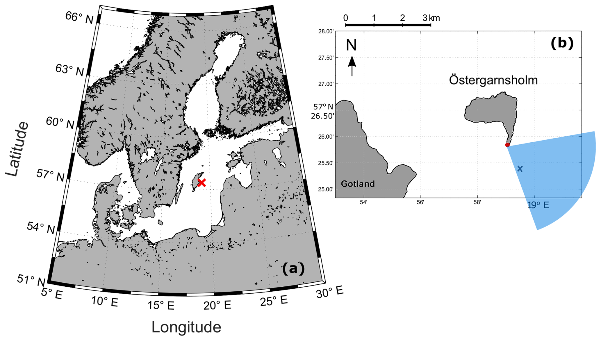
Figure 1(a) Map of the Baltic Sea; the red cross in the central Baltic Sea indicates the location of the Östergarnsholm station. (b) Map of the Östergarnsholm station ca. 4 km off the Gotland Island; the red dot indicates the location of the tower; the blue cross is the location of the mooring with water-side instrumentation (Sect. 2.1.2); the shaded blue area is the so-called “open-sea” sector with wind directions from 80∘ < WD < 160∘ (see Sect. 2.1.1 for details).
2.1.1 Atmospheric data
The tower at Östergarnsholm was instrumented with high-frequency sensors for continuous turbulence measurements. Air–sea CO2 fluxes were calculated using the fluctuations of the vertical wind component, measured by a CSAT3 3D sonic anemometer (Campbell Scientific, Inc., Logan, UT, USA), and the fluctuations in the atmospheric CO2 molar densities, which were measured with an open-path gas analyser model LI-7500A (from 2013 to 2017) or model LI-7500RS (between 2017 and 2021) (LI-COR, Inc., Lincoln, NE, USA). For details about the flux calculations, see Sect. 2.2. The sonic anemometer and gas analyser were located at a height of 9 m from the tower base (i.e. 10.4 m with respect to the mean sea level) and had a sampling rate of 20 Hz. In addition to the high-frequency data, profile measurements of wind speed, wind direction, and temperature at 7, 12, 14, 20, and 29 m height were carried out at 1 Hz and averaged over 30 min periods. Relative humidity, atmospheric pressure, incoming solar radiation, and precipitation were also measured at the site.
The measurements at the Östergarnsholm site have been found to be representative of open-sea or coastal conditions depending on the wind direction (Rutgersson et al., 2020). Only data with wind directions from the southeast (80∘ < WD < 160∘), representing open-sea conditions, were included in the analysis of the current study (Fig. 1b). For this wind sector, it was considered that no disturbances occurred in the tower measurements due to flow distortion and that the wave field was not affected by the shallowing of the seafloor (Högström et al., 2008). Furthermore, the biogeochemical water properties and hydrographical features were assumed to be spatially homogeneous along this sector (Rutgersson et al., 2008, 2020), ensuring that the water-side measurements were representative of the flux footprint of the tower. A more detailed description of the Östergarnsholm site can be found in Rutgersson et al. (2020).
The flux footprint is a function used to characterize the contributions of the sources and sinks per unit area to the total flux measured at a certain point. Based on this mathematical concept, it is possible to associate the fluxes measured at a specific height with the surface exchange of any scalar (e.g. Kormann and Meixner, 2001). According to the flux footprint estimates (Kljun et al., 2015), in this study the source/sink area of the fluxes from the open-sea sector measured at 10.4 m height was located a few hundred metres upwind of the tower. Figure 2 shows the spatial distribution of the flux contributions (in m−2) for different atmospheric stability conditions. For unstable and neutral conditions, the main flux source/sink was found as a localized area near the tower, while for stable conditions, the source/sink contributions per unit area were smaller closer to the tower and rather spread over a larger region.
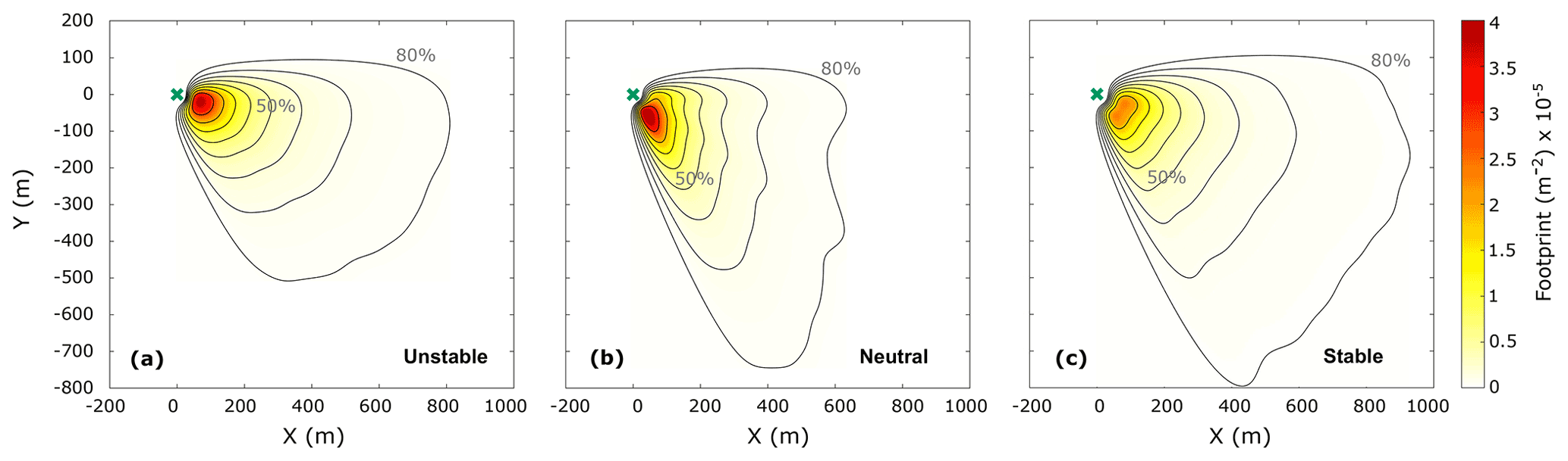
Figure 2Average footprint distribution for (a) unstable, (b) neutral, and (c) stable atmospheric conditions. X and Y represent the horizontal domain with origin (0,0) at the tower's location (green cross), and the contours represent the percentage of the source area from 10 %–80 %. The flux footprint (in colour) shows the spatial distribution of the contributions per unit area to the total FCO2 (in m−2). The footprint was calculated using the model developed by Kljun et al. (2015) using all data available for the open-sea sector between mid-2013 and 2020.
The atmospheric stability was represented as , where z is the measurement height and L is the Monin–Obukhov length. The latter is given by , where u* is the friction velocity, Θ is the potential temperature, g=9.81 m s−2 is the acceleration due to gravity, κ=0.4 is the von Kármán constant, and is the buoyancy flux. The sonic temperature, Ts, was considered to be almost equal to the virtual temperature, Tv, which is often used for buoyancy flux calculations (Aubinet et al., 2012). Following Sjöblom and Smedman (2002), we use z=10.4 m as the mean measurement height with respect to the mean sea level. Here, unstable conditions were defined as , near-neutral conditions as , and stable conditions as .
2.1.2 Water-side measurements
Water-side measurements were carried out continuously at a mooring located 1 km southeast of the tower (see Fig. 1b). At the mooring, seawater temperature and partial pressure of CO2 were measured every 30 min using a SAMI-CO2 sensor (Sunburst Sensors, LLC, MT, USA) at a depth of 4 m. Additionally, continuous wave measurements were made with a Directional Waverider buoy located 4 km southeast of the tower (outside the domain in Fig. 1b). The Waverider buoy is operated and maintained by the Finnish Meteorological Institute (FMI). In this study, the characteristics of the sea state were represented by the significant wave height (Hs); the wave steepness calculated as , where Lp is the peak wavelength; and the wave age, , where Cp is the phase velocity of the waves and U10N is the neutral equivalent wind speed at 10 m height.
Daily data of the mixed-layer depth (MLD) from the Baltic Sea Physics Reanalysis product provided by the Copernicus Marine Environment Monitoring System (CMEMS) (Von Schuckmann et al., 2016) were used as an indicator of the vertical mixing in the water column and for the water-side convection calculations (Rutgersson and Smedman, 2010; Norman et al., 2013b). These data are freely available from the CMEMS website at http://marine.copernicus.eu/services-portfolio/access-to-products/ (last access: 24 February 2022).
2.2 Data processing
High-frequency data obtained at the Östergarnsholm site (Sect. 2.1.1) were used for FCO2 calculations using the eddy covariance method (Baldocchi et al., 1988; Aubinet et al., 2012) and the subsequent gas transfer velocity analysis. The turbulent fluctuations for the flux calculation (described below) were obtained following a Reynolds decomposition using an average period of 10 min. These averages were calculated as block averages from the linearly detrended time series of the 20 Hz data. The turbulent fluctuations were used to calculate variances and covariances. Other statistical moments were also calculated from the turbulent fluctuations and used as part of the quality control.
The raw wind-speed components were transformed to Earth-system coordinates and corrected using a double rotation (Kaimal and Finnigan, 1994). Wind speed and direction were calculated from the corrected components to avoid effects caused by the tilting of the sonic anemometer. Following the convention, measured wind speeds were adjusted to a neutral equivalent wind speed at 10 m height (U10N). Only wind directions representing open-sea conditions were used in the analysis; see Sect. 2.1.1 for details. Only periods with the three consecutive 10 min averages from 80 ∘ < WD < 160 ∘ (i.e. open-sea sector) were included. Data with wind speeds lower than 2 m s−1 were excluded from the FCO2 calculations.
The performance of the gas analyser was evaluated based on the relative signal strength indicator (RSSI). Following Nilsson et al. (2018), we used the variance of the RSSI () to remove low-quality data. The variance was calculated over the 10 min periods, and only data with were considered in the analysis. Additionally, thresholds of different statistical parameters were used to ensure the homogeneity of the data and avoid outliers. Data were excluded if the absolute value of the fourth-order moment of the CO2 signal was higher than 100 ppm4 to filter out outliers and if the variance of the vertical wind speed was m2 s−2 to exclude unrealistically low values of the vertical wind variance (low-turbulence conditions).
According to the eddy covariance method, the FCO2 values were calculated from
where ρa is the mean density of dry air and the term represents the time-averaged covariance between the turbulent fluctuations of the vertical wind component (w) and the dry mole fraction of the gas (c). The FCO2 values were calculated over 30 min periods by averaging three consecutive 10 min periods fulfilling all the quality control steps. The flux was directly calculated from the CO2 dry mole fraction (i.e. mole fraction of CO2 relative to dry air) obtained from the measured molar densities of CO2 relative to the ambient air. By using this direct conversion method (Sahlée et al., 2008), the corrections for dilution effects (Webb et al., 1980) were avoided. A description of the direct conversion method and detailed discussion can be found in Sahlée et al. (2008). Fluxes with magnitudes below a minimum detection limit of ± 0.05 were removed. This limit was empirically defined to avoid data with a low signal-to-noise ratio. In addition to FCO2, enthalpy fluxes were also estimated from the turbulent measurements as the sum of the sensible () and latent () heat fluxes. Furthermore, cases with high-relative-humidity conditions (RH > 95 %) were excluded to avoid data possibly affected by condensation on the instruments.
The gas transfer velocity, k, was calculated from Eq. (1) using the calculated FCO2 (Eq. 2). The solubility constant (K0) was determined from the relationship suggested by Weiss (1974) using a constant salinity value of 7 PSU and in situ water temperature from the SAMI sensor. Changes in the salinity, which oscillates between 6.5 and 7.5 PSU in this region of the Baltic (e.g. Wesslander et al., 2010; Rutgersson et al., 2020), are not expected to have significant effects on the solubility. The ΔpCO2 was obtained from measured with the SAMI sensor and calculated from the molar densities obtained with the gas analyser. Periods with 50 µatm were excluded from the analysis. Furthermore, during conditions of strong water-side stratification, measurements carried out at 4 m depth might not be representative of the air–sea CO2 fluxes measured at the tower. Therefore, all the data occurring during strongly stratified conditions according to the in situ observations were not considered in the analysis. Data were removed when the water-side temperature gradient (ΔTw) was larger than 1 ∘C. The ΔTw was defined as the difference between Tw measured at 4 m depth and the near-surface water temperature (Tns) measured at 0.35 m depth with the Waverider buoy. The calculated k values were adjusted to a reference Schmidt number (Sc) to compensate for temperature and salinity effects. The adjusted gas transfer velocity (k660) was given by , where Sc=660 corresponds to the Schmidt number of CO2 at 20 ∘C for seawater (S=35 ‰), and Sc was the Schmidt number calculated with the corresponding in situ water temperature (Tw) for each data point.
The final data set, after quality control processing, consisted of 3477 FCO2 data points and 1349 k660 data points. These numbers of data correspond to 18.7 % and 15 %, respectively, out of the total number of data available for the open-sea sector (18 625 FCO2 and 8974 k660 data points). Further information about the rejection rates of each quality control criterion can be found in Appendix B.
The calculated k660 values were used to study the effect of water-side and atmospheric control mechanisms on air–sea CO2 exchange. A wind-speed relationship (kwind) was calculated as the cubic (best) fit to the bin-averaged k660, using equidensity bins based on the wind-speed percentiles, and used to obtain a normalized gas transfer velocity defined as . The use of a normalized gas transfer velocity allowed the analysis of mechanisms on k660, in addition to the effect of wind speed. For the analysis, the data were divided into three different wind-speed regimes from light breeze to moderate gale. The thresholds for these regimes were chosen depending on the expected conditions at the sea surface according to the Beaufort scale (Barua, 2005). Low wind speeds were defined as U10N<6 m s−1, covering conditions of light to moderate breeze; only ripples and small waves causing little disturbance on the surface were expected under these conditions. Intermediate conditions representing moderate breezes included wind speeds of m s−1. Finally, relatively high wind-speed conditions were defined as U10N>8 m s−1 when moderate to long waves were expected and whitecaps and sea spray were likely to be observed; these wind speeds correspond to fresh breeze to moderate gale.
3.1 Oceanic and meteorological conditions: the annual cycle
The annual cycle, obtained using the 9 years of data (2013–2021), showed a seasonal pattern in both and (Fig. 3a). The variability was small, at least when compared to the variability in . The lowest values were observed during the late summer and autumn with values often below 380 µatm. Higher values occurred during winter, reaching 440 µatm, while the monthly means of oscillated around 410 µatm. An increasing trend in was observed during the study period (not shown); a linear regression using the monthly averages suggested an increase of 0.2 ppm per month, which corresponds to a total increase of approximately 20 ppm during the 9-year period. Both the trend and the seasonal variability in were masked by the variability in (Fig. 3a). A strong seasonal pattern was observed for , with values higher than those in the atmosphere during winter and lower during summer. The seasonality in in the Baltic Sea has been recognized to be strongly modulated by biological activity (Thomas and Schneider, 1999a; Wesslander et al., 2010). Here, the lowest reached values below 100 µatm during the summer of 2018. The highest values of occurred during the winters of 2018/19 and 2019/20 with observed values higher than 800 µatm. Furthermore, lower summer values were observed in the last 3 years in comparison to previous years. In this way, the inter-annual variability of was mostly noticeable in terms of an increasing amplitude of the seasonal cycle during the last few years.
The monthly means of FCO2 showed a seasonal cycle with positive fluxes during the winter and negative fluxes during the summer (Fig. 3b). This seasonal pattern in the flux was consistent with the thermodynamic forcing (i.e. ), which suggested an upward transport during the winter and downward transport during the summer. However, a high variability in the half-hourly data was observed year-round.

Figure 3Annual cycle of (a) CO2 partial pressure (pCO2) in the seawater and in the atmosphere and (b) air–sea CO2 fluxes from eddy covariance. The dots represent the half-hourly values, and the solid lines show the monthly averages.
The atmospheric and water-side variables describing the physical characteristics showed clear seasonal cycles (Fig. 4). However, a large scatter was observed from the individual half-hourly values, thus highlighting the large variability and heterogeneity of the environment. The monthly means of wind speed and significant wave height (Hs) were higher during the autumn and winter, in comparison to the summer (Fig. 4a and b). However, short-term events with high winds (U10N>10 m s−1) and waves (Hs∼ 3 m) were observed during all seasons. The temperature gradient (, Fig. 4c) showed that from September to February (day of year (DOY) 250–50) the ocean was, on average, 1.5 ∘C warmer than the overlying air (i.e. positive gradient). During late spring, the atmospheric temperature was warmer than the seawater with an average ΔT of −1 ∘C. The enthalpy flux showed mean monthly values of 0–75 W m−2 (Fig. 4d). The monthly means of relative humidity (RH, Fig. 4e) ranged between 60 % and 85 % throughout the year, but a large scatter was observed, particularly during autumn and winter (DOY 250–50), when moderately low values of RH (<40 %) often occurred.
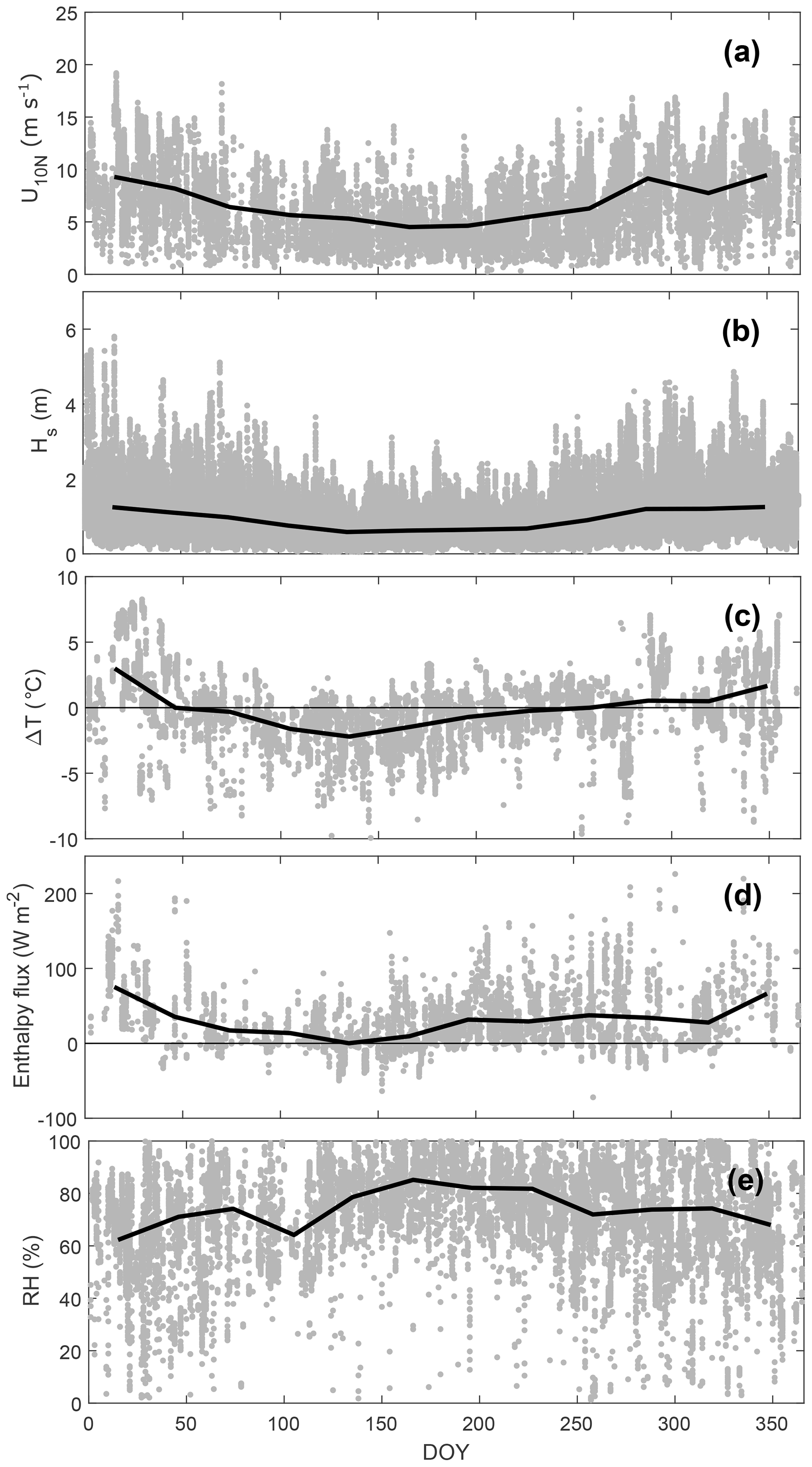
Figure 4Annual cycle of (a) 10 m neutral wind speed, (b) significant wave height, (c) temperature gradient (), (d) enthalpy flux, and (e) relative humidity. The dots are the half-hourly values, and the solid black lines represent the monthly average of each parameter.
3.2 The gas transfer velocity
The gas transfer velocity, k660, followed – on average – an increasing relationship with wind speed. The best fit calculated using the mean k660 values for each equidensity bin (130 data points) indicated a cubic relationship with wind speed, following a general agreement with other commonly used parametrizations (Fig. 5). Even when the best fit to the bin means (kwind) seemed to accurately represent the average behaviour of k660 as a function of wind speed (R2=0.97), a large scatter in the k660 half-hourly values was observed. Only ∼30 % of such variability in the half-hourly values was explained by a wind-speed relationship (not shown).
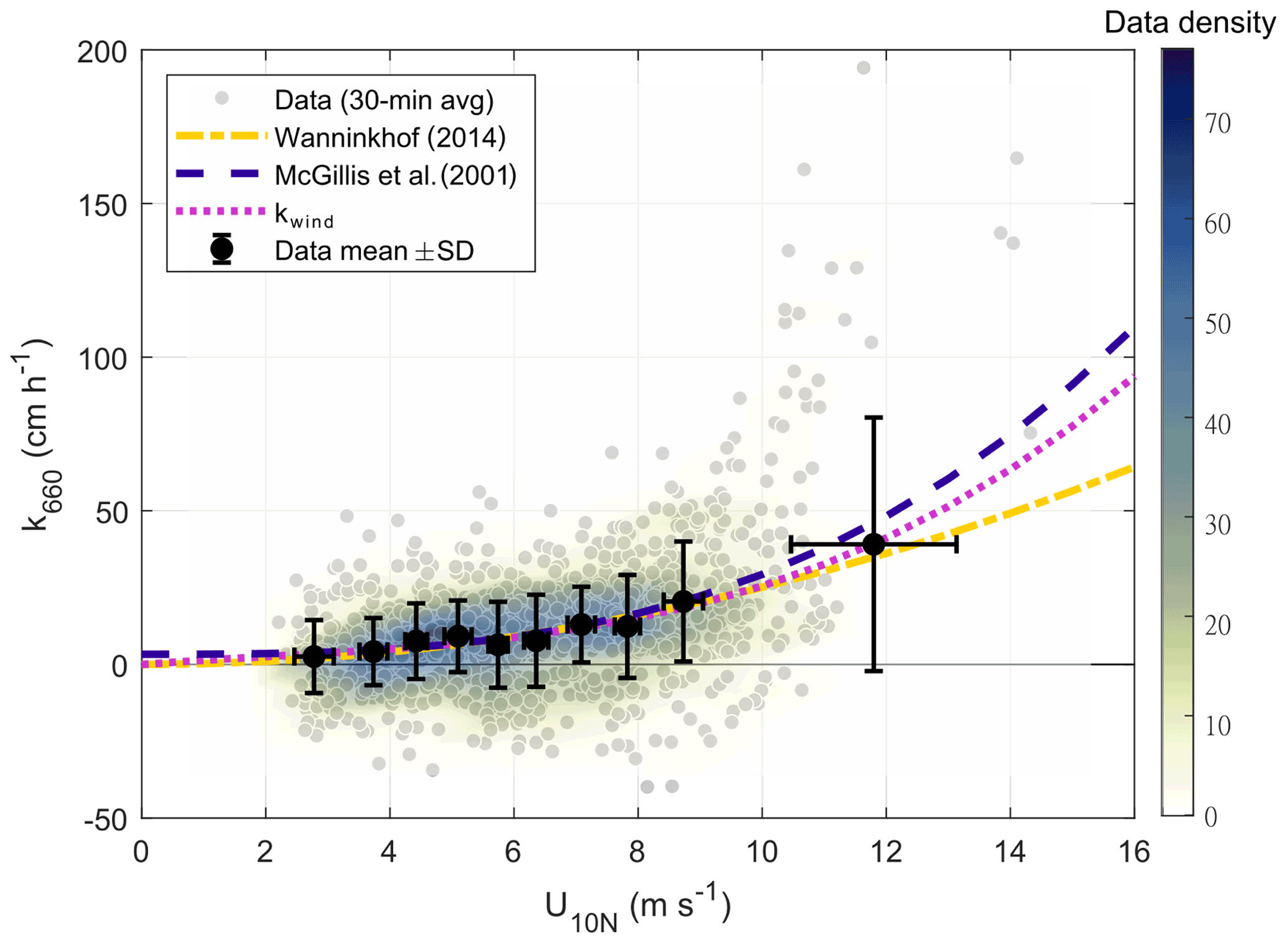
Figure 5Gas transfer velocity for CO2 (adjusted to a Schmidt number of 660) as a function of the 10 m neutral wind speed. The grey dots represent the half-hourly values of k660 for the 9-year period from 2013 to 2021. The black dots and bars represent the k660 mean values and standard deviations, respectively, calculated for equidensity bins based on the wind-speed percentiles; the best fit to the means is shown as the dotted pink line (kwind). For reference, quadratic (Wanninkhof, 2014) and cubic (McGillis et al., 2001) wind-based parametrizations are included. The colours in the shaded area represent the data density (in counts) with a grid bin size of 1 m s−1 by 10 cm h−1.
We used the gas transfer velocity normalized by the wind-based relationship (i.e. ) to evaluate the effect of individual atmospheric and water-side processes on the gas exchange. Boxplots showing the statistical summary for equidensity bins defined based on the distribution of the normalized gas transfer velocity as a function of each of the parameters were used to evaluate . Based on this analysis, we further identified the conditions inducing the strongest variability in k660 under different wind-speed regimes (Sect. 2.2), presented in Sect. 3.2.1 to 3.2.3. The entire set of figures of can be found in Appendix A.
3.2.1 Controls on k660 under high-wind-speed conditions
Under high-wind-speed conditions (U10N>8 m s−1), water-side properties such as MLD and the wave field were found to be associated with the behaviour of the gas transfer velocity. Furthermore, not only was ΔpCO2 the driver of the flux defining the direction of the transport, but the characteristics of the gradient were also connected to the efficiency of the exchange. Thus, ΔpCO2 was considered a water-side control here due to the importance of in modulating the variability in the gradient, in comparison to the rather constant values of (see Sect. 3.1).
Particular conditions of the water-side parameters were found to be linked to k660 values higher than those suggested by the wind-speed relationship (i.e. ), while the rest of the time, wind speed seemed to better describe the behaviour of k660 (i.e. ) (Fig. 6). Moderately positive gradients, with ΔpCO2 of the order of 50–100 µatm, were associated with significantly higher values (Fig. 6a), while under conditions of strong positive and negative gradients, k660 followed the wind-based relationship; smaller gradients (both positive and negative) showed the largest variability. Furthermore, at these relatively high wind-speed conditions (U10N>8 m s−1), the water column was well mixed, and, while some scatter is observed, the largest values of k660 seemed to be related to a deep mixed layer (Fig. 6c). The combined effect of ΔpCO2 and MLD was strongly modulated by seasonal patterns. During the winter, strong and persistent vertical mixing occurred along with positive ΔpCO2 (Fig. 3a). During the summer, shallower MLD and negative ΔpCO2 were observed. Consistently, the probability distribution function showed a higher probability of positive ΔpCO2 during the high-wind-speed regime (Fig. A1a) together with a wide distribution of MLD (Fig. A1b), suggesting winter conditions prevailed during a large proportion of the high-wind-speed regime. On the contrary, a higher probability of negative ΔpCO2 and shallower MLD occurred during low wind speeds.
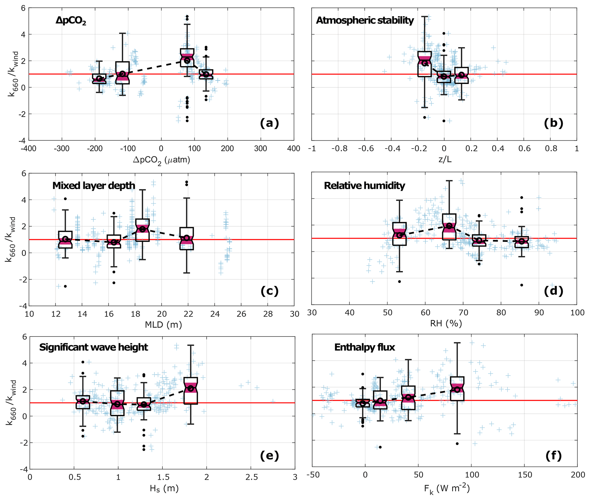
Figure 6Normalized gas transfer velocity () under high-wind-speed conditions (U10N> 8 m s−1) as a function of (a) ΔpCO2, (b) atmospheric stability (), (c) mixed-layer depth (MLD), (d) relative humidity (RH), (e) significant wave height (Hs), and (f) total enthalpy flux (Fk). The crosses represent the individual half-hourly values. The boxplots give a statistical summary for equidensity bins defined based on the distribution of as a function of each of the parameters (see Appendix A). The median, first, and third quartiles are represented in each box; the whiskers represent the minimum and maximum values, and the black dots represent the outliers; the notches highlighted in pink indicate the median's 95 % confidence interval. The open circles linked with a dashed line indicate the bin means, and the horizontal red line indicates .
In addition to ΔpCO2 and MLD, the characteristics of the wave field were – to some extent – associated with an enhanced gas exchange. In particular, the highest significant wave heights (Hs>1.5 m) were consistent with the largest values of (Fig. 6e). Low values of wave steepness () were observed even at the highest wind speeds, with maximum values of 0.06 (Fig. A2e), much lower than the theoretical wave-breaking threshold (Stokes, 1880), while the small values of the wave age, (Fig. A2f), indicated growth of the wave field caused by the wind forcing over the surface. Thus, this suggests the prevalence of locally generated waves (i.e. wind sea) under these wind-speed conditions.
Atmospheric conditions such as atmospheric stability, relative humidity, and the total enthalpy flux were also associated with the gas exchange efficiency. In terms of the atmospheric stability, a clear enhancement of k660 was observed during unstable conditions in comparison to kwind (Fig. 6b). Meanwhile, during neutral and stable conditions, no significant difference was observed between k660 and kwind. Relative humidity below 70 % was consistent with , while during higher RH, the scatter in the data was low and k660 was well represented by kwind. Furthermore, an increasing trend was observed in terms of the total enthalpy flux, with higher k660 values observed when high enthalpy fluxes occurred.
Based on the analysis presented in Fig. 6, we identified a set of conditions that were associated with enhanced values of k660. These conditions were characterized by positive ΔpCO2, strong water-side mixing, and dry air (RH < 70 %) during unstable atmospheric stratification. A wave field with Hs>1.5 m further enhanced the gas exchange. Gas transfer velocities that were higher than predicted, not only by kwind but also by other commonly used parametrizations, were observed under these specific conditions (Fig. 7). These enhanced conditions were observed particularly during high wind speeds but also during the intermediate regime and to a much lesser extent during the low-wind-speed conditions. When these data were excluded from the analysis, k660 was better represented by U10N following a quadratic relationship (R2=0.62). Furthermore, the enhanced k660 (blue dots in Fig. 7) showed a wind-speed dependency of higher order (cubic) and R2=0.57.
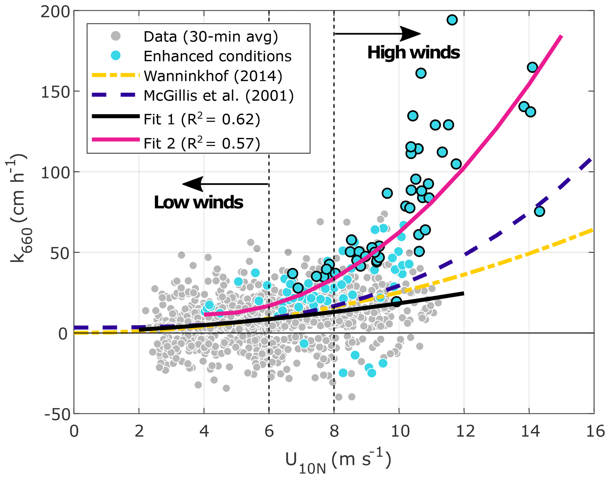
Figure 7Gas transfer velocity for CO2 (adjusted to a Schmidt number of 660) as a function of the 10 m neutral wind speed. The dots represent the half-hourly values of k660. The blue dots represent k660 under enhanced conditions (see text for details), while the blue dots with a black edge indicate cases where Hs>1.5 m. The black line represents the best fit (quadratic) to the data excluding the enhanced cases (only grey dots), while the pink line is the best fit to the enhanced data (only blue dots). For reference, quadratic (Wanninkhof, 2014) and cubic (McGillis et al., 2001) wind-based parametrizations are included. The wind-speed regimes are separated by vertical dashed lines.
3.2.2 Controls on k660 under low-wind-speed conditions
Under low-wind-speed conditions (U10N≤6 m s−1), the scatter of the data was even larger than under higher wind speeds. Water-side parameters such as ΔpCO2, MLD, and water-side convection helped explain part of the variability observed. Gas transfer velocities higher than predicted by kwind were observed for both positive and negative gradients, showing that only under very strong negative gradients ( µatm) was the gas exchange lower than expected by the wind-speed relationship (Fig. 8a). Under these calmer wind-speed conditions, the values of MLD were generally low (Fig. A1b), with the lowest (MLD < 15) values showing a larger scatter in k660 (Fig. A1k). The pattern of ΔpCO2 and MLD was consistent with the seasonal cycle, where shallow MLD, typical of the summer months, can hinder the downward transport of CO2 into the sea (negative ΔpCO2). The wave field showed smaller (Hs<1 m) and less steep waves. Under these conditions, the waves tended to be older (), indicating a larger proportion of swell waves in comparison to the locally generated waves observed at higher wind speeds. The characteristics of the wave field did not seem to induce any deviation of k660 with respect to kwind at low wind speeds (Fig. A2).
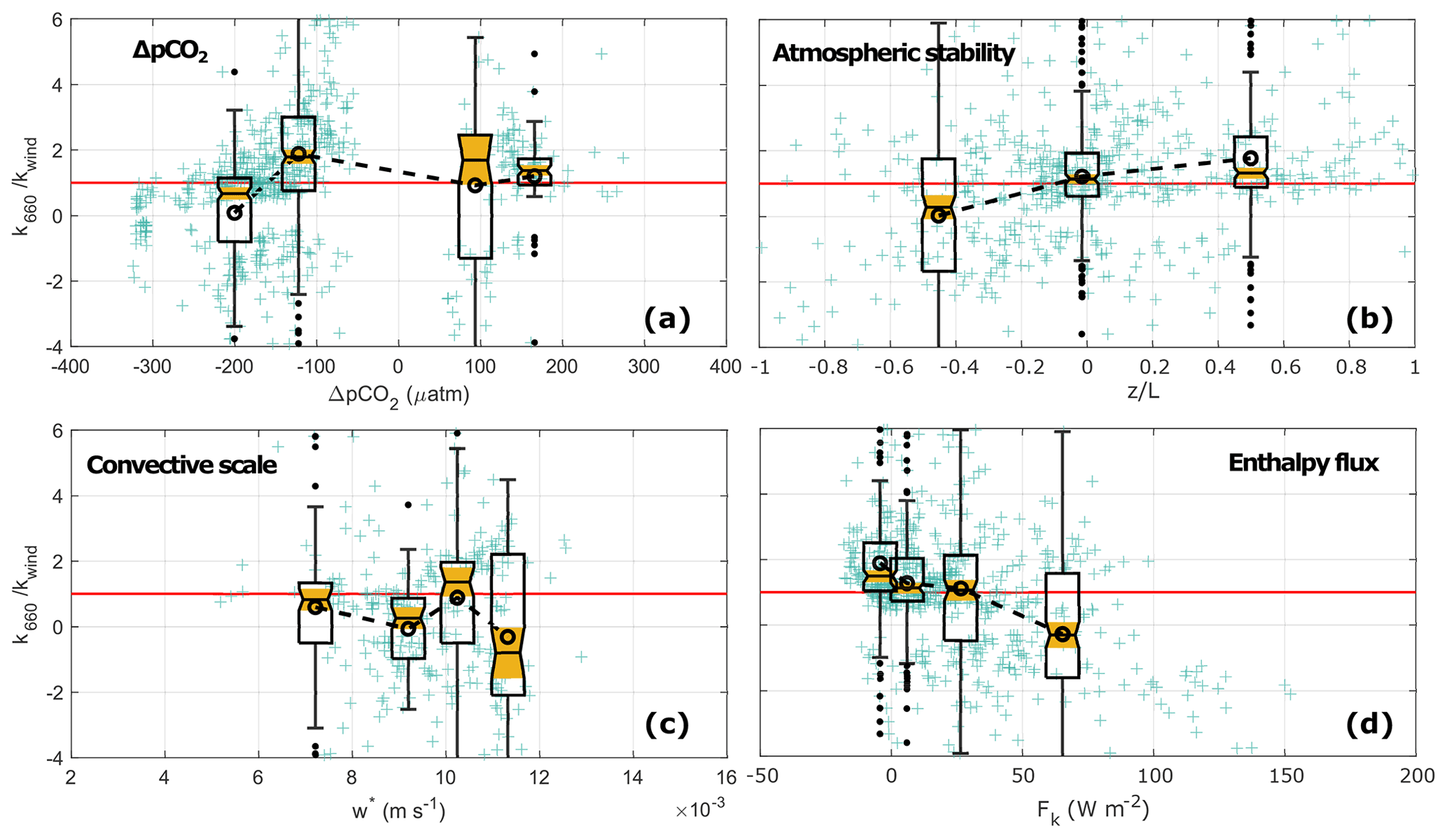
Figure 8Normalized gas transfer velocity () under low-wind-speed conditions (U10N≤6 m s−1) as a function of (a) ΔpCO2, (b) atmospheric stability (), (c) the water-side convective scale (w*) under unstable atmospheric conditions, and (d) enthalpy flux (Fk). The crosses represent the individual half-hourly values. The boxplots give a statistical summary for equidensity bins defined based on the distribution of as a function of each of the parameters (see Appendix A). The median, first, and third quartiles are represented in each box; the whiskers represent the minimum and maximum values, and the black dots represent the outliers; the notches highlighted in yellow indicate the median's 95 % confidence interval. The open circles linked with a dashed line indicate the bin means, and the horizontal red line indicates .
In addition to ΔpCO2 and the MLD, atmospheric stability and the water-side convective scale (w*, as defined in Jeffery et al., 2007) were relevant parameters used to explain at least part of the variability in k660. On average, lower k660 values than expected by kwind during unstable atmospheric conditions and a high water-side convective scale were observed (Fig. 8b and c). However, large variability was observed under these conditions. Meanwhile, kwind seemed to better represent the behaviour of k660 under neutral and stable conditions, as well as during lower magnitudes of the water-side convective scale. Under low-wind-speed conditions, large enthalpy fluxes were associated with (Fig. 8d).
Further analysis of the data during low wind speeds and unstable atmospheric conditions showed that water-side convection can enhance the gas exchange. Particularly during winter, when persistent cooling of the sea surface was expected (ΔT>0), enhanced values of k660 were observed at low and intermediate wind speeds associated with high values of w* (Figs. 9a and 10). On the contrary, low values of w* were predominant during the summer months and linked to low values of k660 (Figs. 9b and 10). Furthermore, some relatively high values of w* were observed during the summer, associated with a large proportion of the negative k660 values observed. Under neutral and stable atmospheric conditions, water-side convection is not a relevant mechanism (Rutgersson and Smedman, 2010; Rutgersson et al., 2011; Norman et al., 2013b).
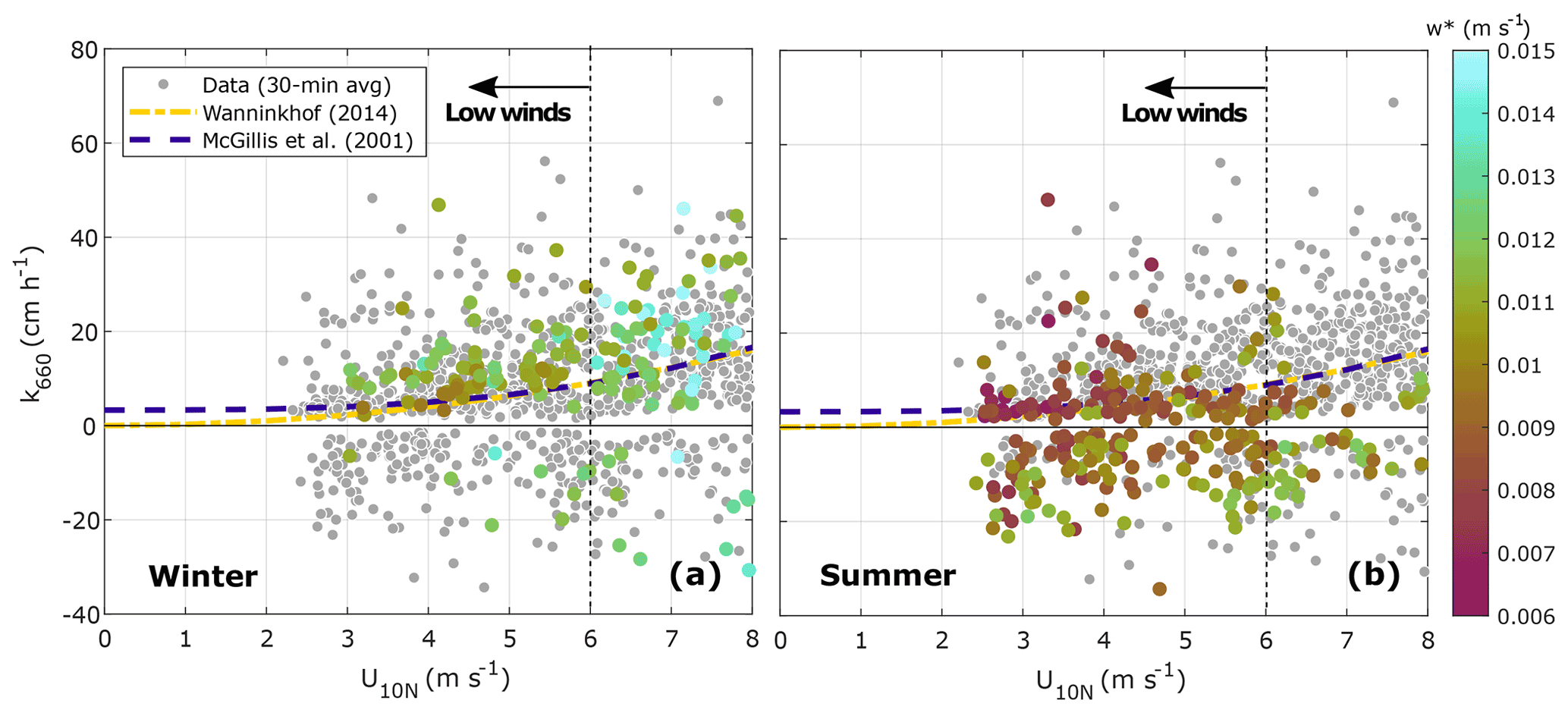
Figure 9Gas transfer velocity for CO2 (adjusted to a Schmidt number of 660) as a function of the 10 m neutral wind speed during (a) winter and (b) summer. The dots represent the half-hourly values of k660. The colour represents the water-side convective scale (w*) for data under unstable atmospheric conditions, calculated according to Rutgersson and Smedman (2010). The wind-speed regimes are separated by a vertical dashed line.
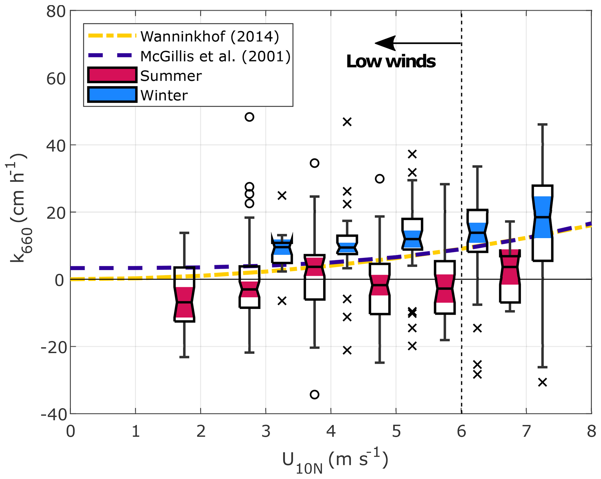
Figure 10Boxplots of the gas transfer velocity for CO2 (adjusted to a Schmidt number of 660) during unstable atmospheric conditions as a function of the 10 m neutral wind speed during summer (pink) and winter (blue). The median, first, and third quartiles are represented in each box; the whiskers represent the minimum and maximum values, and the circles and crosses represent the outliers; the notches highlighted in colour indicate the median's 95 % confidence interval. The wind-speed regimes are separated by a vertical dashed line.
The rest of the scattered data which occurred during negative ΔpCO2 and shallow MLD cannot be explained by water-side convection or any other parameter assessed in this study. Furthermore, the interpretation of these data should be taken with some caution as the strong stratification, relatively weak ΔpCO2, and the possibility of strong heterogeneity in terms of the biogeochemical properties might hinder our capacity to calculate k660 from and FCO2.
3.2.3 Controls on k660 in the intermediate-wind-speed range
Wind speeds between 6 and 8 m s−1 were considered the intermediate range here. As such, the characteristics of this intermediate-wind-speed range were found to be a transition in terms of the physical conditions between the low and high wind speeds (see figures in Appendix A). The wave field showed waves with an average Hs of 0.9 m, in comparison to the 1.4 and 0.6 m of the high-wind-speed and low-wind-speed regimes, respectively. However, wave steepness and wave age in intermediate winds showed average values of and , similar to the mean values of and observed at higher wind speeds. However, no clear effect of the wave field was observed on k660 (Fig. A2g, h, and i). Both the wave field and the wind speed seemed to cause stronger mixing as larger values of MLD reaching the entire water column (ca. 25 m) were observed under the transition range in contrast to the more persistent stratification at lower wind speeds (Fig. A1b). Values of MLD during these intermediate wind speeds were still lower, on average, than those observed during the high-wind-speed regime. Meanwhile, large values of w* suggest the mixing caused by water-side convective processes during unstable atmospheric conditions might be relevant at the intermediate wind speeds, in particular, during the winter (Fig. 9a).
We used 9 years of eddy-covariance-based FCO2 data to evaluate the effect of different control mechanisms on air–sea CO2 gas exchange. By using this long record, we were able to capture the seasonal and inter-annual variability of the FCO2 and other parameters relevant to the gas exchange (Sect. 3.1), as well as directly assess controls on k660 (Sect. 3.2). Direct FCO2 measurements over long periods are necessary in order to resolve the effect of multiple parameters on the gas exchange on both short-term and long-term (several years) scales.
The empirically derived k660 values showed, on average, a similar wind-speed dependency to two wind-based parametrizations, the quadratic relationship from Wanninkhof (2014) and the cubic relationship from McGillis et al. (2001) (Fig. 5). These parametrizations were used as references, and further comparison with the data presented here is beyond the scope of the study. Furthermore, we considered that the use of other commonly used parametrizations (e.g. Wanninkhof and McGillis, 1999; Nightingale et al., 2000; Ho et al., 2006) would show similar results. Based on the results presented here, we showed, on the one hand, that a wind-based model with a similar pattern to those developed for larger basins and open-ocean conditions was an accurate representation (R2=0.97) of the mean k660. On the other hand, the scatter of the half-hourly data suggested that a large proportion of the short-term variability in k660 was not explained by variations in the wind speed. Previous studies have already pointed out the relevance of mechanisms other than the wind as controls on air–sea gas exchange in heterogeneous environments such as marginal and coastal seas (e.g. Upstill-Goddard, 2006; Gutiérrez-Loza et al., 2021). Here, based on the analysis of atmospheric and water-side parameters, we identified conditions associated with enhanced k660 during high-wind-speed and low-wind-speed conditions.
We identified a set of conditions that were associated with enhanced values of k660 at intermediate and high wind speeds (Fig. 7). These conditions were characterized by positive ΔpCO2 (i.e. winter conditions), unstable atmospheric stratification, strong vertical mixing in the water column (deep MLD), and low relative humidity. These conditions, affecting the upward fluxes during the winter months, resulted in an even more pronounced enhancement of k660 when the wave field presented high significant wave heights (Hs>1.5 m). We suggest here that the high k660 values observed can be potentially explained by the effect of sea spray on air–sea CO2 flux under the aforementioned conditions. In this hypothesis, the role of atmospheric parameters as control mechanisms is a key factor for the otherwise water-side-controlled CO2 exchange across the sea surface. Unstable atmospheric conditions, for example, have been previously found to be associated with enhanced CO2 transport (Andersson et al., 2019; Van Dam et al., 2021), possibly due to additional small-scale turbulence, as suggested by Andersson et al. (2019). However, in this study we found that none of the individual parameters had a clear effect on k660, and it was rather the combination of these parameters that led to the specific conditions enhancing the exchange, potentially due to effective evaporation of droplets with relatively high .
The characteristics of the wave field are one of the most important parameters involved in the air–sea gas transfer directly affecting the conditions of the interface. However, the effect of waves on gas exchange has been very seldom studied in coastal regions (e.g. Gutiérrez-Loza et al., 2018). We analysed different parameters describing the wave field (significant wave height, wave steepness, and wave age) and their effect on the gas transfer velocity. At high wind speeds, the waves were found to be locally generated by the wind (i.e. wind sea), which made it hard to separate the effect of the waves from that of the wind. The wave climate in the Baltic Sea is characterized by a predominant short wind sea and scarce long swell (Soomere, 2022). Furthermore, the effect of swell waves was not relevant under high-wind-speed conditions, and while at lower wind speeds some effect from swell could be expected, such an effect was partly excluded here as wind speeds lower than 2 m s−1 were removed from the analysis. Values of wave steepness suggested that there was no systematic wave breaking. However, empirical knowledge of the study site suggests the presence of breaking, particularly of the smallest/youngest waves. These waves are not expected to generate significant bubble entrainment into the upper layer of the sea, but generation of sea spray is expected at the highest wind speeds.
The role of sea spray as a control mechanism of the air–sea gas exchange has been reported before (Andreas et al., 2016, 2017). The impact of a broken surface caused by wave breaking and whitecapping has been shown to cause an asymmetric transport due to the injection of bubbles into the ocean enhancing the negative (downward) fluxes (Woolf, 1997; Leighton et al., 2018). However, the potential effect of such processes on positive fluxes is still unclear. Here, we found that the increase in the k660 was associated with the ocean-to-atmosphere (upward) transport in what we suggest is the effect of sea spray. This effect was clearly affected by the seasonal variability as the increased k660 was observed during the winter months, when dry and cold air (colder than the ocean) is common (Fig. 4c and e). During the winter months positive CO2 gradients prevail and positive gas and heat fluxes are most often observed. High enthalpy fluxes were observed during the conditions enhancing k660; however, the mechanisms through which the transport is enhanced might be different as heat and moisture are air-side controlled. Nonetheless, the increased evaporation rates most probably found during low relative humidity and unstable conditions might also play a role in CO2 transport. Dedicated analysis of the effect of bubbles and sea spray in coastal regions is still necessary, particularly at high latitudes, where strong seasonality may cause significant differences in the forcing mechanisms modulating the influx and efflux of gas into/from the ocean (see Sect. 3.1). Further data under these particular conditions are necessary to establish a better understanding of the effect of sea-spray-mediated gas fluxes as it can be a relevant mechanism modulating FCO2 at global scales.
Under calm wind-speed conditions, with U10N<6 m s−1, the effect of water-side convection was found to be relevant to explaining the larger values of k660 during unstable atmospheric conditions at these wind speeds. Previous studies have shown the effect of convective processes on the gas transfer in the Baltic Sea (Rutgersson and Smedman, 2010; Norman et al., 2013b). The same studies showed that the water-side convective processes are not relevant under stable and neutral conditions, as well as at wind speeds higher than 8 m s−1. Here, we found the effect of water-side convection to be strongly seasonal (Figs. 9 and 10), where a clear enhancement due to water-side convection occurred during the winter. During the summer, low values of w* seemed to mostly follow the wind-speed relationships. However, intermediate values of w* can be linked with most of the negative k660 observed during low and intermediate wind speeds (Fig. 9b), thus indicating that it was during these unstable conditions when the mismatch between the observed fluxes and ΔpCO2 occurred. Further investigation is necessary in order to evaluate the effect of water-side convection at other temporal scales (i.e. diurnal variability), as well as the potential implications for FCO2 at larger spatial scales.
In addition to the processes analysed in this study, there are other mechanisms which are relevant for the gas exchange in the Baltic Sea at different temporal and spatial scales. The occurrence of upwelling events can be up to 25 %–30 % in some regions of the Baltic Sea (Lehmann et al., 2012). Norman et al. (2013a) found that the effect of these events on the annual mean FCO2 can reach up to 25 % for the Baltic Sea conditions. Upwelling is not expected to be relevant for the wind directions analysed in this study; however, we recognize that the effect of upwelling in the area can be important and can have implications for the observed inter-annual variability. Furthermore, using the parametrization suggested by Pereira et al. (2018) based on skin temperature, we calculated a rough estimate of the effect of surfactants on our long-term k660. The results suggest an overall effect of merely −0.1 %, suggesting a very small reduction in k660 when surfactants are taken into account. A detailed analysis of the effect of surface films is beyond the scope of this study. Nevertheless, we recognize that this process might be particularly relevant in coastal seas and other shallow bodies of water. The analysis of the effect of sea ice, precipitation, Langmuir circulation, and other processes in the Baltic Sea is still pending.
Eddy covariance data have been increasingly used in marine environments to study air–sea gas exchange (e.g. McGillis et al., 2001; Miller et al., 2010; Andersson et al., 2016; Gutiérrez-Loza et al., 2019). Although eddy covariance measurements have greatly contributed to the better understanding of gas exchange processes, some caveats still exist regarding this methodology. Dong et al. (2021) recently published a thorough analysis regarding the uncertainties associated with air–sea eddy covariance and subsequent gas transfer velocity calculations. In that study, the total uncertainty was calculated as , where δFR is the random error component and δFS is the systematic bias. According to their estimates, the total propagated bias (estimated from the individual sources) represented a flux uncertainty of 7.5 %. The largest potential source of bias was the motion of the ship, followed by the imperfect calibration of the sensors and the effect of the inlet tubes (i.e. for closed-path gas analysers); other potential sources of bias such as airflow distortion, instrument separation, and water vapour cross-sensitivity were found to be negligible. An additional 5 % bias due to insufficient sampling time resulted in a total systematic error of 9 %. Furthermore, Dong et al. (2021) found that the contributions of the random errors (δFR) represented a much larger contribution (20 %–50 %) to the total flux uncertainty, with the low-CO2-flux regions presenting the largest uncertainty. According to Dong et al. (2021), the total flux uncertainty (δF) represents 10 % of the variance in k660. Moreover, using data from the Östergarnsholm station, Rutgersson et al. (2008) estimated an uncertainty of 17 % associated with the eddy covariance fluxes (using two open-path gas analysers), while the contributions of the other terms involved in the gas transfer velocity calculation, i.e. the solubility parameter and ΔpCO2, were estimated to be 1 % and 4 %, respectively. The total instrumental errors estimated in Rutgersson et al. (2008), which do not consider any methodological biases, resulted in a total uncertainty of 20 % in the gas transfer velocity estimates. Assuming that the values presented by Dong et al. (2021) are applicable to our study and considering that the land-based station is not subject to platform movement or the effect of inlet tubes, a rough estimate of the flux uncertainty caused by systematic bias gives δFS<6.4 %. Furthermore, based on the monthly mean FCO2 (Fig. 3), Östergarnsholm is in the “high-CO2-flux” regime (> 10 ) during most of the year and therefore lies in the lower range (∼ 20 %) of the random uncertainty values. Based on these values of random error and systematic bias, a total uncertainty value of ∼ 20 % associated with the flux measurements can be assumed. The propagated error associated with the gas transfer velocity is, therefore, also of the order of ∼ 20 %, in agreement with previous estimates from Östergarnsholm (Rutgersson et al., 2008).
In addition to the uncertainties discussed above, in this study we identified two major limitations that further affected the analysis. The first limitation was the large number of data that were removed from the analysis due to quality control (Sect. 2.2 and Appendix B). The criterion excluding the largest number of data was the wind-direction selection (open-sea sector) criterion that excluded ca. 85 % of the total data (Table B1). Relaxing this criterion would significantly increase the number of data used for the k660 analysis. However, it would also mean including fluxes associated with more heterogeneous regions where the measured water properties might not necessarily be representative of FCO2 (see Rutgersson et al., 2020), hence introducing larger uncertainties into the k660 estimates. Furthermore, the criterion regarding the signal quality of the gas analyser () was only fulfilled by 36.7 % of the flux data. Most of the data that were removed due to the low-signal criterion occurred during precipitation events or in very high wind speeds, when droplets land on the optical windows of the gas analyser. Gutiérrez-Loza et al. (2021) found that precipitation (rain) increased the net CO2 uptake by 4 % in the Baltic Sea during 2009–2011, while Ashton et al. (2016) found that the effect of rain can lead to a 6 % increase in the ocean uptake, globally. By removing the data due to low signal strength, the effects of precipitation remained unaccounted for in the analysis presented here, as well as fluxes under high-wind-speed conditions (above 12–14 m s−1), where strong mixing, bubble injection, and sea spray might be important controls on air–sea gas exchange (e.g. Blomquist et al., 2017; Bell et al., 2017). Removing small fluxes (i.e. ) due to the gas analyser detection limit might bias the net flux estimates. Therefore, we limited this study to the analysis of the half-hourly values and general seasonal patterns; however, conclusions about whether the region was an overall sink or source of CO2 were avoided. Finally, the potential effect of swell on the CO2 exchange at very low wind speeds was not accounted for, given that wind speeds lower than 2 m s−1 were removed from the analysis. The other criteria (see Table B1) were expected to cause very small biases, if any, in the data. The probability distribution of the quality-controlled data set showed similar patterns compared to the initial data set (before quality control) for each parameter used in the analysis (i.e. ΔpCO2, wind speed, wave properties, etc.), hence indicating that the reduced data set used for the analysis was a good representation of the conditions observed in the study area over the 9-year measurement period.
The second caveat was the large number of negative k660 values observed (Fig. 5). These data fulfilled every step of the quality control process, and therefore, there was no methodological reason to exclude these values from the data set. However, further investigation is needed to understand the source of these data and whether or not there is a viable physical explanation. We considered that part of the negative values observed here can be attributed to the inherent turbulent characteristics of eddy covariance measurements. Furthermore, at low wind speeds, conditions hindering k660 calculations (e.g. strong stratification), as well as instrumental and set-up limitations such as measurement response time and depth, might become relevant. Furthermore, processes not accounted for such as chemical enhancement and surfactants (e.g. Ribas-Ribas et al., 2018), might also play a role in the number and distribution of negative k660 values observed.
Regardless of the length of our data set, we still found three major limitations when addressing the effect of forcing mechanisms on air–sea gas exchange: (1) the use of a land-based station provides significant advantages, but it hinders the evaluation of the spatial variability in the exchange; (2) the intrinsic characteristics of the eddy covariance technique, in combination with the exclusion of wind directions not representative of open-sea conditions, resulted in a patchy data set with significant gaps throughout the time series; and (3) a limited number of data at high wind speeds (U10N>10 m s−1) were recorded, which hindered the analysis and increased the uncertainties under those critical wind conditions. The results presented here provide significant insights into the air–sea gas exchange and its variability. Nevertheless, the limitations are still large and continued effort from the scientific community is required.
Global coastal oceans and marginal seas comprise one of the most vulnerable environments subjected to the effect of climate change and anthropogenic pressures (IPCC, 2014). Understanding the role of these regions in the global carbon cycle has become an essential aspect in order to address the challenges of the current and future climates. In this sense, the Baltic Sea can be seen as a test basin which provides a wide variety of physical and biogeochemical conditions. At the same time, the carbon system of the Baltic Sea has been relatively well documented (e.g. Kuliński and Pempkowiak, 2011; Schneider and Müller, 2018), and the region has been a relevant study area in terms of mitigation and environmental management (Reusch et al., 2018). The analysis and results presented here can be relevant for other marginal seas and coastal areas, while the potential effect of sea spray and water-side convection is certainly relevant at global scales, and further investigation is encouraged.
We presented a large data set of directly measured air–sea CO2 fluxes by eddy covariance from a land-based station in the Baltic Sea. The forcing mechanisms acting on the surface of the ocean and their relative effect on the gas exchange can widely vary depending on the wind speed. Therefore, the air–sea gas exchange, controlled by such forcing mechanisms, can also be expected to be affected in different ways depending on the wind-speed regime. We investigated the effect of the water-side and atmospheric conditions on the gas transfer velocity under relatively high wind-speed, intermediate-wind-speed, and low-wind-speed regimes.
At high wind speeds (U10N>8 m s−1), large k660 values were observed in what we identified to be cold and dry air, under unstable atmospheric conditions. We suggest, based on these results, that sea spray might be one of the most effective mechanisms enhancing air–sea CO2 fluxes under these conditions, partly due to large evaporation rates. The effect of the wave field was particularly evident in terms of the significant wave height, with high gas transfer velocity values occurring when large values of Hs were observed. However, the effect of the wave field was not completely decoupled from the effect of the wind, given that most of the waves were locally generated. Under low-wind-speed conditions (U10N<6 m s−1), water-side convection was the only parameter explaining part of the variability in k, particularly during the winter. Intermediate wind speeds showed mixed behaviour; thus, we defined these wind speeds as a transition range. Under these intermediate-wind-speed conditions, the effect of sea spray is still relevant, similarly to the behaviour in higher winds, while convective processes enhanced k660 during winter, as they do at lower wind speeds.
A wind-based model, showing a similar pattern to currently existing wind-based parametrizations, was shown to adequately represent the average behaviour of k660. However, further investigation of parameters affecting the seasonal and inter-annual variability of the fluxes is needed to improve our understanding of air–sea gas exchange and adequately represent k660 at shorter timescales. Similarly, a detailed analysis of bubble-mediated and sea-spray-mediated fluxes is needed to contribute to the understanding of CO2 fluxes in the coastal regions and other heterogeneous environments where the asymmetric behaviour of the transport might have strong implications.
The full set of figures showing the normalized gas transfer velocity () vs. each of the parameters analysed in this study is presented here. The parameters are divided into water-side control mechanisms (Fig. A1), wave field characteristics (Fig. A2), and atmospheric control mechanisms (Fig. A3). Each figure also includes the probability distribution function (PDF) of each variable for high, intermediate, and low wind speeds to highlight the difference between the wind regimes.
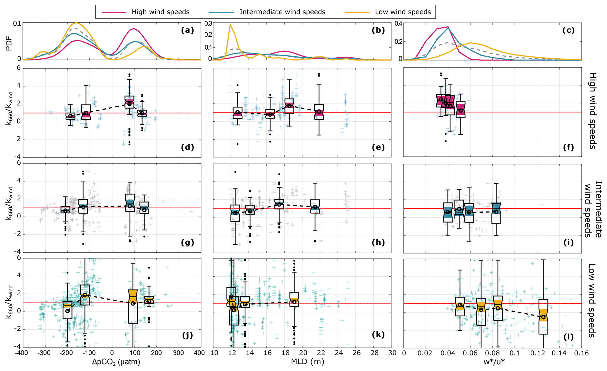
Figure A1Water-side control mechanisms: ΔpCO2 (left), mixed-layer depth (centre), and water-side convective scale normalized with the friction velocity () (right). Top panels (a), (b), and (c) show the probability distribution function (PDF). Panels (d) to (l) show the normalized gas transfer velocity () under high (upper), intermediate (middle), and low (lower) wind speeds. The crosses represent the individual half-hourly values. The boxplots give a statistical summary for equidensity bins defined based on the distribution of as a function of each of the parameters. The median, first, and third quartiles are represented in each box; the whiskers represent the minimum and maximum values, and the black dots represent the outliers; the notches highlighted in yellow indicate the median's 95 % confidence interval. The open circles linked with a dashed line indicate the bin means, and the horizontal red line indicates .
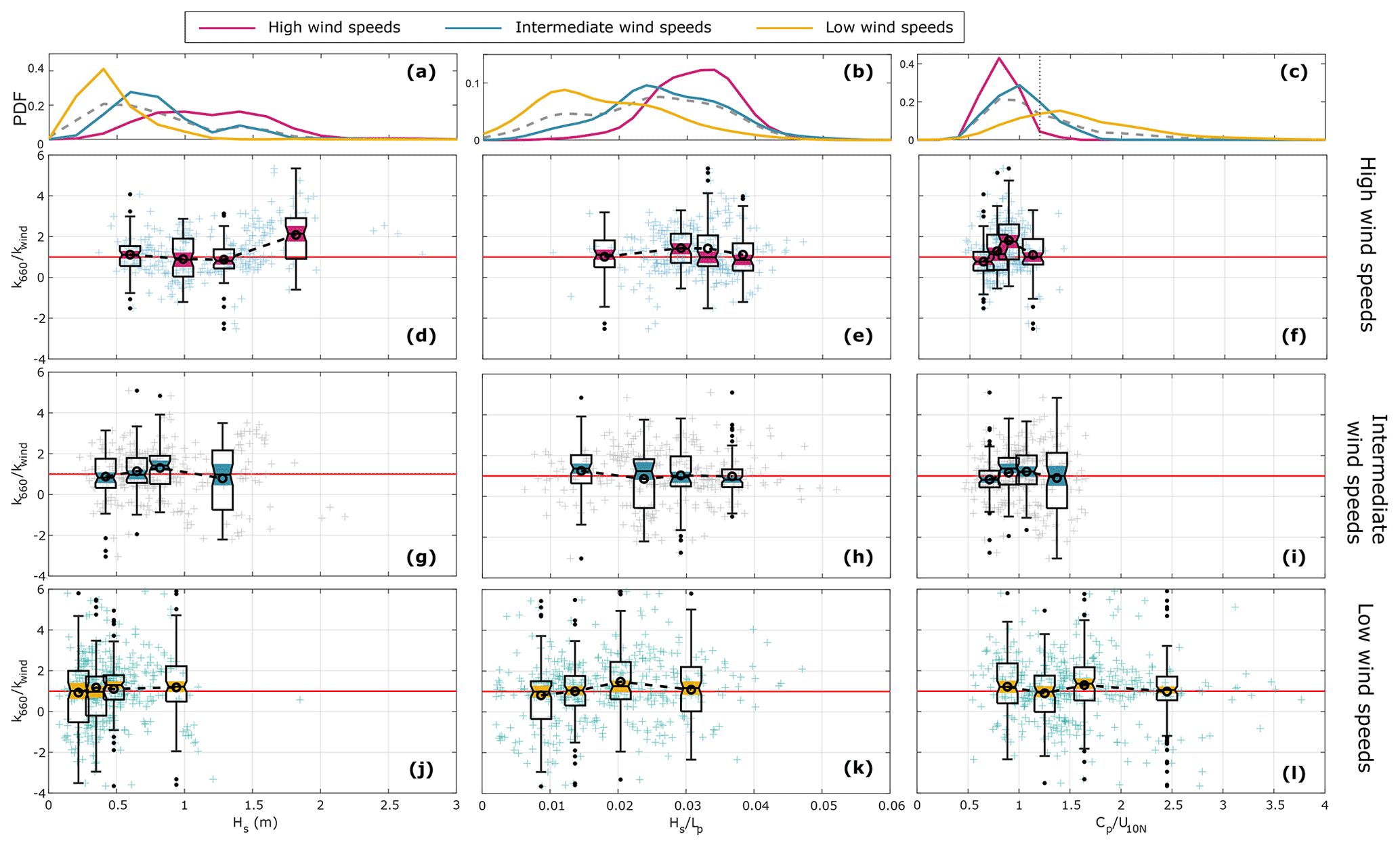
Figure A2Same as in Fig. A1 for wave field characteristics: significant wave height (left), wave steepness (centre), and wave age (right).

During the 9-year record between 2013 and 2021, we recorded 125 001 FCO2 data points and 66 475 k660 data points out of the maximum possible of 157 776 (half hours in 9 years). However, strict quality control and post-processing analysis were necessary to ensure that only high-quality data were used for the flux calculations using the eddy covariance method (see Sect. 2.2). A significant number of data were removed from the data set based on these criteria. Information about the relative importance of each criterion of the quality control is presented in Table B1.
The wind-direction selection criterion (i.e. using only the open-sea sector) is the procedure that rejects the largest number of data from the data set (Table B1). Considering that the total number of data for this sector, before the quality control, was 18 625 FCO2 and 8974 k660 data points, the final data set consisted of 18.7 % and 15.0 % of the open-sea initial data for FCO2 and k660, respectively. This corresponded to 3477 and 1349 data points, respectively.
Table B1Percentage of data that successfully fulfil each individual quality control criterion. The percentages are relative to the total recorded number of data (100 % = 125 001 for FCO2 and 100 % = 66 475 for k660).
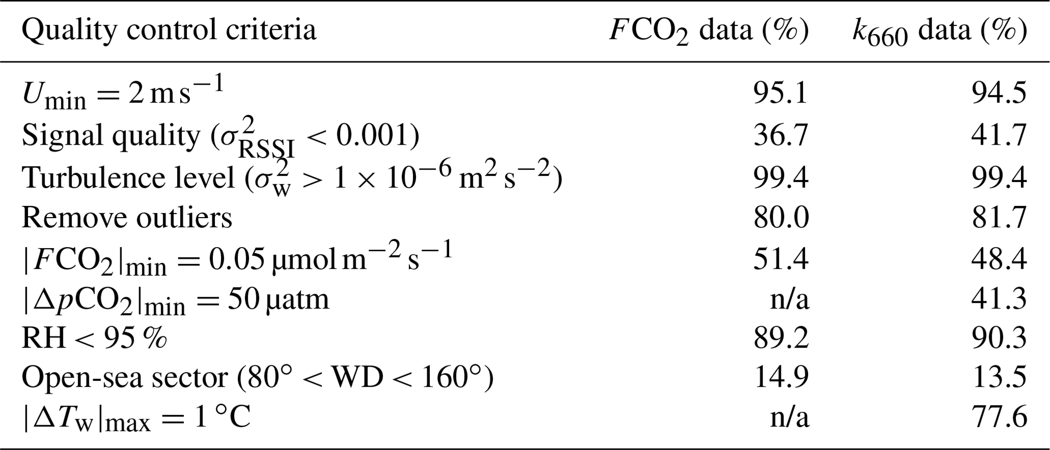
n/a: not applicable; i.e., the corresponding criterion has no impact on the resulting number of data.
The raw data supporting the conclusions of this paper are available upon request.
LGL, MBW, ES, and AR were involved in the conceptualization of the project. AR was in charge of the project administration and funding acquisition. The formal analysis was carried out by LGL with the support of EN. LGL, MBW, EN, and AR participated in the continuous maintenance of the Östergarnsholm station and data acquisition. LGL wrote the original draft with contribution from all the co-authors.
The contact author has declared that none of the authors has any competing interests.
Publisher’s note: Copernicus Publications remains neutral with regard to jurisdictional claims in published maps and institutional affiliations.
The ICOS station Östergarnsholm is funded by the Swedish Research Council (Vetenskapsrådet) and Uppsala University. The wave data were provided by Heidi Pettersson from the Finnish Meteorological Institute (FMI), to whom the authors are grateful.
This research has been supported by Vetenskapsrådet (grant nos. 2012-03902 and 2013-02044) and Uppsala Universitet.
This paper was edited by Peter Landschützer and reviewed by Bryce Van Dam and one anonymous referee.
Andersson, A., Rutgersson, A., and Sahlée, E.: Using eddy covariance to estimate air–sea gas transfer velocity for oxygen, J. Mar. Syst., 159, 67–75, 2016. a
Andersson, A., Sjöblom, A., Sahlée, E., Falck, E., and Rutgersson, A.: Enhanced air–sea exchange of heat and carbon dioxide over a high Arctic Fjord during unstable very-close-to-neutral conditions, Bound.-Lay. Meteorol., 170, 471–488, 2019. a, b
Andreas, E., Vlahos, P., and Monahan, E.: The potential role of sea spray droplets in facilitating air-sea gas transfer, in: IOP conference series: earth and environmental science, Vol. 35, p. 012003, IOP Publishing, https://doi.org/10.1088/1755-1315/35/1/012003, 2016. a, b
Andreas, E. L., Vlahos, P., and Monahan, E. C.: Spray-mediated air-sea gas exchange: the governing time scales, Journal of Marine Science and Engineering, 5, 60, 2017. a
Ashton, I. G., Shutler, J. D., Land, P. E., Woolf, D. K., and Quartly, G. D.: A sensitivity analysis of the impact of rain on regional and global sea–air fluxes of CO2, PloS one, 11, e0161105, https://doi.org/10.1371/journal.pone.0161105, 2016. a, b
Aubinet, M., Vesala, T., and Papale, D.: Eddy covariance: a practical guide to measurement and data analysis, Springer Science & Business Media, https://doi.org/10.1007/978-94-007-2351-1, 2012. a, b
Baldocchi, D. D., Hincks, B. B., and Meyers, T. P.: Measuring biosphere–atmosphere exchanges of biologically related gases with micrometeorological methods, Ecology, 69, 1331–1340, 1988. a
Barua, D. K.: Beaufort wind scale, Encyclopedia of Coastal Science, Dordrecht, Springer Netherlands, 2005. a
Bell, T. G., Landwehr, S., Miller, S. D., de Bruyn, W. J., Callaghan, A. H., Scanlon, B., Ward, B., Yang, M., and Saltzman, E. S.: Estimation of bubble-mediated air–sea gas exchange from concurrent DMS and CO2 transfer velocities at intermediate–high wind speeds, Atmos. Chem. Phys., 17, 9019–9033, https://doi.org/10.5194/acp-17-9019-2017, 2017. a, b
Blomquist, B. W,, Brumer, S. E., Fairall, C. W., Huebert, B. J., Zappa, C. J., Brooks, I. M., Yang, M., Bariteau, L., Prytherch, J., Hare, J. E., Czerski, H., Matei, A., and Pascal, R. W.: Wind speed and sea state dependencies of air–sea gas transfer: Results from the High Wind speed Gas exchange Study (HiWinGS), J. Geophys. Res.-Ocean., 122, 8034–8062, 2017. a, b
Borges, A. V., Delille, B., and Frankignoulle, M.: Budgeting sinks and sources of CO2 in the coastal ocean: Diversity of ecosystems count, Geophys. Res. Lett., 32, L14601, https://doi.org/10.1029/2005GL023053, 2005. a
Brumer, S. E., Zappa, C. J., Blomquist, B. W., Fairall, C. W., Cifuentes-Lorenzen, A., Edson, J. B., Brooks, I. M., and Huebert, B. J.: Wave-related Reynolds number parameterizations of CO2 and DMS transfer velocities, Geophys. Res. Lett., 44, 9865–9875, 2017. a
Chen, C.-T. A., Huang, T.-H., Chen, Y.-C., Bai, Y., He, X., and Kang, Y.: Air–sea exchanges of CO2 in the world's coastal seas, Biogeosciences, 10, 6509–6544, https://doi.org/10.5194/bg-10-6509-2013, 2013. a
Ciais, P., Sabine, C., Bala, G., Bopp, L., Brovkin, V., Canadell, J., Chhabra, A., DeFries, R., Galloway, J., Heimann, M., et al.: Carbon and other biogeochemical cycles, in: Climate change 2013: the physical science basis. Contribution of Working Group I to the Fifth Assessment Report of the Intergovernmental Panel on Climate Change, edited by: Stocker, T., Qin, D., Plattner, G.-K., Tignor, M., Allen, S., Boschung, J., Nauels, A., Xia, Y., Bex, V., and Midgley, P., 465–570, Cambridge University Press, 2013. a
Dong, Y., Yang, M., Bakker, D. C. E., Kitidis, V., and Bell, T. G.: Uncertainties in eddy covariance air–sea CO2 flux measurements and implications for gas transfer velocity parameterisations, Atmos. Chem. Phys., 21, 8089–8110, https://doi.org/10.5194/acp-21-8089-2021, 2021. a, b, c, d
Erickson III, D. J.: A stability dependent theory for air-sea gas exchange, J. Geophys. Res.-Ocean., 98, 8471–8488, 1993. a, b
Friedlingstein, P., Jones, M. W., O'Sullivan, M., Andrew, R. M., Bakker, D. C. E., Hauck, J., Le Quéré, C., Peters, G. P., Peters, W., Pongratz, J., Sitch, S., Canadell, J. G., Ciais, P., Jackson, R. B., Alin, S. R., Anthoni, P., Bates, N. R., Becker, M., Bellouin, N., Bopp, L., Chau, T. T. T., Chevallier, F., Chini, L. P., Cronin, M., Currie, K. I., Decharme, B., Djeutchouang, L. M., Dou, X., Evans, W., Feely, R. A., Feng, L., Gasser, T., Gilfillan, D., Gkritzalis, T., Grassi, G., Gregor, L., Gruber, N., Gürses, Ö., Harris, I., Houghton, R. A., Hurtt, G. C., Iida, Y., Ilyina, T., Luijkx, I. T., Jain, A., Jones, S. D., Kato, E., Kennedy, D., Klein Goldewijk, K., Knauer, J., Korsbakken, J. I., Körtzinger, A., Landschützer, P., Lauvset, S. K., Lefèvre, N., Lienert, S., Liu, J., Marland, G., McGuire, P. C., Melton, J. R., Munro, D. R., Nabel, J. E. M. S., Nakaoka, S.-I., Niwa, Y., Ono, T., Pierrot, D., Poulter, B., Rehder, G., Resplandy, L., Robertson, E., Rödenbeck, C., Rosan, T. M., Schwinger, J., Schwingshackl, C., Séférian, R., Sutton, A. J., Sweeney, C., Tanhua, T., Tans, P. P., Tian, H., Tilbrook, B., Tubiello, F., van der Werf, G. R., Vuichard, N., Wada, C., Wanninkhof, R., Watson, A. J., Willis, D., Wiltshire, A. J., Yuan, W., Yue, C., Yue, X., Zaehle, S., and Zeng, J.: Global Carbon Budget 2021, Earth Syst. Sci. Data, 14, 1917–2005, https://doi.org/10.5194/essd-14-1917-2022, 2022. a, b
Gutiérrez-Loza, L., Ocampo-Torres, F. J., and García-Nava, H.: The Effect of Breaking Waves on CO2 Air–Sea Fluxes in the Coastal Zone, Bound.-Lay. Meteorol., 168, 343–360, 2018. a
Gutiérrez-Loza, L., Wallin, M. B., Sahlée, E., Nilsson, E., Bange, H. W., Kock, A., and Rutgersson, A.: Measurement of air-sea methane fluxes in the Baltic Sea using the eddy covariance method, Front. Earth Sci., 7, 93, https://doi.org/10.3389/feart.2019.00093, 2019. a
Gutiérrez-Loza, L., Wallin, M. B., Sahlée, E., Holding, T., Shutler, J. D., Rehder, G., and Rutgersson, A.: Air–sea CO2 exchange in the Baltic Sea – A sensitivity analysis of the gas transfer velocity, J. Mar. Syst., 222, 103603, https://doi.org/10.1016/j.jmarsys.2021.103603, 2021. a, b
Ho, D. T., Law, C. S., Smith, M. J., Schlosser, P., Harvey, M., and Hill, P.: Measurements of air–sea gas exchange at high wind speeds in the Southern Ocean: Implications for global parameterizations, Geophys. Res. Lett., 33, https://doi.org/10.1029/2006GL026817, 2006. a
Högström, U., Sahlée, E., Drennan, W. M., Kahma, K. K., Smedman, A.-S., Johansson, C., Pettersson, H., Rutgersson, A., Tuomi, L., Zhang, F., and Johansson, M.: Momentum fluxes and wind gradients in the marine boundary layer: A multi platform study, Boreal Environ. Res., 13, 475–502, 2008. a, b
Honkanen, M., Müller, J. D., Seppälä, J., Rehder, G., Kielosto, S., Ylöstalo, P., Mäkelä, T., Hatakka, J., and Laakso, L.: The diurnal cycle of pCO2 in the coastal region of the Baltic Sea, Ocean Sci., 17, 1657–1675, https://doi.org/10.5194/os-17-1657-2021, 2021. a
Jacobs, E., Bittig, H. C., Gräwe, U., Graves, C. A., Glockzin, M., Müller, J. D., Schneider, B., and Rehder, G.: Upwelling-induced trace gas dynamics in the Baltic Sea inferred from 8 years of autonomous measurements on a ship of opportunity, Biogeosciences, 18, 2679–2709, https://doi.org/10.5194/bg-18-2679-2021, 2021. a
Jeffery, C., Woolf, D., Robinson, I., and Donlon, C.: One-dimensional modelling of convective CO2 exchange in the Tropical Atlantic, Ocean Modell., 19, 161–182, 2007. a
Jessup, A., Zappa, C. J., and Yeh, H.: Defining and quantifying microscale wave breaking with infrared imagery, J. Geophys. Res.-Ocean., 102, 23145–23153, 1997. a
Kaimal, J. C. and Finnigan, J. J.: Atmospheric boundary layer flows: their structure and measurement, Oxford University Press, ISBN: 0-19-506239-6, 1994. a
Kljun, N., Calanca, P., Rotach, M. W., and Schmid, H. P.: A simple two-dimensional parameterisation for Flux Footprint Prediction (FFP), Geosci. Model Dev., 8, 3695–3713, https://doi.org/10.5194/gmd-8-3695-2015, 2015. a, b
Kormann, R. and Meixner, F. X.: An analytical footprint model for non-neutral stratification, Bound.-Lay. Meteorol., 99, 207–224, 2001. a
Kuliński, K. and Pempkowiak, J.: The carbon budget of the Baltic Sea, Biogeosciences, 8, 3219–3230, https://doi.org/10.5194/bg-8-3219-2011, 2011. a, b
Kuliński, K., Rehder, G., Asmala, E., Bartosova, A., Carstensen, J., Gustafsson, B., Hall, P. O. J., Humborg, C., Jilbert, T., Jürgens, K., Meier, H. E. M., Müller-Karulis, B., Naumann, M., Olesen, J. E., Savchuk, O., Schramm, A., Slomp, C. P., Sofiev, M., Sobek, A., Szymczycha, B., and Undeman, E.: Biogeochemical functioning of the Baltic Sea, Earth Syst. Dynam., 13, 633–685, https://doi.org/10.5194/esd-13-633-2022, 2022. a
Laruelle, G. G., Dürr, H. H., Slomp, C. P., and Borges, A. V.: Evaluation of sinks and sources of CO2 in the global coastal ocean using a spatially-explicit typology of estuaries and continental shelves, Geophys. Res. Lett., 37, L15607, https://doi.org/10.1029/2010GL043691, 2010. a
Laruelle, G. G., Lauerwald, R., Pfeil, B., and Regnier, P.: Regionalized global budget of the CO2 exchange at the air-water interface in continental shelf seas, Global Biogeochem. Cy., 28, 1199–1214, 2014. a
Lehmann, A., Myrberg, K., and Höflich, K.: A statistical approach to coastal upwelling in the Baltic Sea based on the analysis of satellite data for 1990–2009, Oceanologia, 54, 369–393, 2012. a
Leighton, T. G., Coles, D. G., Srokosz, M., White, P. R., and Woolf, D. K.: Asymmetric transfer of CO2 across a broken sea surface, Sci. Rep., 8, 1–9, 2018. a
Löffler, A., Schneider, B., Perttilä, M., and Rehder, G.: Air–sea CO2 exchange in the Gulf of Bothnia, Baltic Sea, Cont. Shelf Res., 37, 46–56, 2012. a
McGillis, W. R., Edson, J. B., Hare, J. E., and Fairall, C. W.: Direct covariance air–sea CO2 fluxes, J. Geophys. Res.-Ocean., 106, 16729–16745, 2001. a, b, c, d
Miller, S. D., Marandino, C., and Saltzman, E. S.: Ship-based measurement of air-sea CO2 exchange by eddy covariance, J. Geophys. Res.-Atmos., 115, D02304, https://doi.org/10.1029/2009JD012193, 2010. a
Nightingale, P. D., Malin, G., Law, C. S., Watson, A. J., Liss, P. S., Liddicoat, M. I., Boutin, J., and Upstill-Goddard, R. C.: In situ evaluation of air–sea gas exchange parameterizations using novel conservative and volatile tracers, Global Biogeochem. Cy., 14, 373–387, 2000. a
Nilsson, E., Bergström, H., Rutgersson, A., Podgrajsek, E., Wallin, M. B., Bergström, G., Dellwik, E., Landwehr, S., and Ward, B.: Evaluating humidity and sea salt disturbances on CO2 flux measurements, J. Atmos. Ocean. Technol., 35, 859–875, 2018. a
Norman, M., Parampil, S. R., Rutgersson, A., and Sahlée, E.: Influence of coastal upwelling on the air–sea gas exchange of CO2 in a Baltic Sea Basin, Tellus B, 65, 21831, https://doi.org/10.3402/tellusb.v65i0.21831, 2013a. a, b
Norman, M., Rutgersson, A., and Sahlée, E.: Impact of improved air–sea gas transfer velocity on fluxes and water chemistry in a Baltic Sea model, J. Marine Syst., 111, 175–188, 2013b. a, b, c, d, e
IPCC, 2014: Climate Change 2014: Synthesis Report. Contribution of Working Groups I, II and III to the Fifth Assessment Report of the Intergovernmental Panel on Climate Change, Core Writing Team, edited by: Pachauri, R. K. and Meyer, L. A., IPCC, Geneva, Switzerland, 151 pp., 2014. a
Parard, G., Rutgersson, A., Raj Parampil, S., and Charantonis, A. A.: The potential of using remote sensing data to estimate air–sea CO2 exchange in the Baltic Sea, Earth Syst. Dynam., 8, 1093–1106, https://doi.org/10.5194/esd-8-1093-2017, 2017. a
Pereira, R., Ashton, I., Sabbaghzadeh, B., Shutler, J. D., and Upstill-Goddard, R. C.: Reduced air–sea CO2 exchange in the Atlantic Ocean due to biological surfactants, Nat. Geosci., 11, 492–496, 2018. a, b
Reusch, T. B. H., Dierking, J., Andersson, H. C., et al.: The Baltic Sea as a time machine for the future coastal ocean, Sci. Adv., 4, eaar819, https://doi.org/10.1126/sciadv.aar8195, 2018. a
Ribas-Ribas, M., Helleis, F., Rahlff, J., and Wurl, O.: Air–Sea CO2 exchange in a large annular wind-wave tank and the effects of surfactants, Front. Mar. Sci., 457, https://doi.org/10.3389/fmars.2018.00457, 2018. a, b
Roobaert, A., Laruelle, G. G., Landschützer, P., Gruber, N., Chou, L., and Regnier, P.: The Spatiotemporal Dynamics of the Sources and Sinks of CO2 in the Global Coastal Ocean, Global Biogeochem. Cy., 33, 1693–1714, https://doi.org/10.1029/2019GB006239, 2019. a
Rutgersson, A. and Smedman, A. S.: Enhanced air–sea CO2 transfer due to water-side convection, J. Mar. Syst., 80, 125–134, 2010. a, b, c, d, e, f, g
Rutgersson, A., Smedman, A.-S., and Omstedt, A.: Measured and simulated latent and sensible heat fluxes at two marine sites in the Baltic Sea, Bound.-Lay. Meteorol., 99, 53–84, 2001. a
Rutgersson, A., Norman, M., Schneider, B., Pettersson, H., and Sahlée, E.: The annual cycle of carbon dioxide and parameters influencing the air–sea carbon exchange in the Baltic Proper, J. Mar. Syst., 74, 381–394, https://doi.org/10.1016/j.jmarsys.2008.02.005, 2008. a, b, c, d, e
Rutgersson, A., Norman, M., and Åström, G.: Atmospheric CO2 variation over the Baltic Sea and the impact on air–sea exchange, Boreal Environ. Res., 14, 238–249, 2009. a
Rutgersson, A., Smedman, A., and Sahlée, E.: Oceanic convective mixing and the impact on air–sea gas transfer velocity, Geophys. Res. Lett., 38, L02602, https://doi.org/10.1029/2010GL045581, 2011. a
Rutgersson, A., Pettersson, H., Nilsson, E., Bergström, H., Wallin, M. B., Nilsson, E. D., Sahlée, E., Wu, L., and Mårtensson, E. M.: Using land-based stations for air–sea interaction studies, Tellus A, 72, 1–23, 2020. a, b, c, d, e, f
Sahlée, E., Smedman, A. S., Rutgersson, A., and Högström, U.: Spectra of CO2 and water vapour in the marine atmospheric surface layer, Bound.-Lay. Meteorol., 126, 279–295, 2008. a, b
Schneider, B. and Müller, J. D.: Biogeochemical transformations in the Baltic Sea, Springer, ISBN: 978-3-319-61699-5, 2018. a
Schneider, B., Gülzow, W., Sadkowiak, B., and Rehder, G.: Detecting sinks and sources of CO2 and CH4 by ferrybox-based measurements in the Baltic Sea: Three case studies, J. Mar. Syst., 140, 13–25, 2014. a
Sjöblom, A. and Smedman, A.-S.: The turbulent kinetic energy budget in the marine atmospheric surface layer, J. Geophys. Res.-Ocean., 107, 6–1, 2002. a, b
Smedman, A.-S., Högström, U., Bergström, H., Rutgersson, A., Kahma, K. K., and Pettersson, H.: A case study of air–sea interaction during swell conditions, J. Geophys. Res.-Ocean., 104, 25833–25851, 1999. a
Soloviev, A. and Lukas, R.: The near-surface layer of the ocean: structure, dynamics and applications, Vol. 48, Springer Science & Business Media, Springer, https://doi.org/10.1007/978-94-007-7621-0, 2013. a
Soomere, T.: Numerical simulations of wave climate in the Baltic Sea: a review, Oceanologia, 2022. a
Stokes, G. G.: Supplement to a paper on the theory of oscillatory waves, Mathemat. Phys. Papers, 1, 18, Cambridge University Press, 1880. a
Takahashi, T., Sutherland, S. C., Wanninkhof, R., et al.: Climatological mean and decadal change in surface ocean pCO2, and net sea–air CO2 flux over the global oceans, Deep-Sea Res. Pt. II, 56, 554–577, 2009. a, b
Thomas, H. and Schneider, B.: The seasonal cycle of carbon dioxide in Baltic Sea surface waters, J. Mar. Syst., 22, 53–67, 1999a. a
Thomas, H. and Schneider, B.: The seasonal cycle of carbon dioxide in Baltic Sea surface waters, J. Mar. Syst., 22, 53–67, 1999b. a
Thomas, H., Pempkowiak, J., Wulff, F., and Nagel, K.: The Baltic Sea, in: Carbon and nutrient fluxes in continental margins, 334–346, edited by: Liu, K.-K., Atkinson, L., Quiñones, R., and. Talaue-McManus, L., Springer Science and Business Media, ISBN: 978-3-540-92734-1, 2010. a
Thorpe, S., Osborn, T., Farmer, D., and Vagle, S.: Bubble clouds and Langmuir circulation: Observations and models, J. Phys. Oceanogr., 33, 2013–2031, 2003. a
Upstill-Goddard, R. C.: Air–sea gas exchange in the coastal zone, Estuarine, Coast. Shelf Sci., 70, 388–404, 2006. a
Van Dam, B. R., Lopes, C. C., Polsenaere, P., Price, R. M., Rutgersson, A., and Fourqurean, J. W.: Water temperature control on CO2 flux and evaporation over a subtropical seagrass meadow revealed by atmospheric eddy covariance, Limnol. Oceanogr., 66, 510–527, 2021. a
Von Schuckmann, K., Le Traon, P.-Y., Alvarez-Fanjul, E., Axell, L., Balmaseda, M., Breivik, L.-A., Brewin, R. J. W., Bricaud, C., Drevillon, M., Drillet, Y., et al.: The copernicus marine environment monitoring service ocean state report, J. Operat. Oceanogr., 9, s235–s320, https://doi.org/10.1080/1755876X.2016.1273446, 2016. a
Wanninkhof, R.: Relationship between wind speed and gas exchange over the ocean revisited, Limnol. Oceanogr.- Meth., 12, 351–362, 2014. a, b, c
Wanninkhof, R. and McGillis, W. R.: A cubic relationship between air–sea CO2 exchange and wind speed, Geophys. Res. Lett., 26, 1889–1892, 1999. a
Webb, E. K., Pearman, G. I., and Leuning, R.: Correction of flux measurements for density effects due to heat and water vapour transfer, Quarterly J. Roy. Meteorol. Soc., 106, 85–100, 1980. a
Weiss, R.: Carbon dioxide in water and seawater: the solubility of a non-ideal gas, Mar. Chem., 2, 203–215, 1974. a
Wesslander, K., Omstedt, A., and Schneider, B.: Inter-annual and seasonal variations in the air–sea CO2 balance in the central Baltic Sea and the Kattegat, Cont. Shelf Res., 30, 1511–1521, 2010. a, b
Woolf, D. K.: Bubbles and the air-sea transfer velocity of gases, Atmos.-Ocean, 31, 517–540, 1993. a
Woolf, D. K.: Bubbles and their role in gas exchange, 173–206, Cambridge University Press, ISBN (electronic): 9780511525025, ISBN (print): 9780521017459, 1997. a, b
Woolf, D. K., Shutler, J. D., Goddijn-Murphy, L., Watson, A. J., Chapron, B., Nightingale, P. D., Donlon, C. J., Piskozub, J., Yelland, M. J., Ashton, I., Holding, T., Schuster, U., Girard‐Ardhuin, F., Grouazel, A., Piolle, J.‐F., Warren, M., Wrobel‐Niedzwiecka, I., Land, P. E., Torres, R., Prytherch, J., Moat, B., Hanafin, J., Ardhuin, F., and Paul, F.: Key uncertainties in the recent air–sea flux of CO2, Global Biogeochem. Cy., 33, 1548–1563, https://doi.org/10.1029/2018GB006041, 2019. a
Zhao, D., Toba, Y., Suzuki, Y., and Komori, S.: Effect of wind waves on air–sea gas exchange: Proposal of an overall CO2 transfer velocity formula as a function of breaking-wave parameter, Tellus B, 55, 478–487, 2003. a