Interannual variability of the initiation of the phytoplankton growing period in two French coastal ecosystems

Decadal time series of chlorophyll a concentrations sampled at high and low frequencies are explored to study climate-induced impacts on the processes inducing interannual variations in the initiation of the phytoplankton growing period (IPGP) in early spring. We specifically detail the IPGP in two contrasting coastal temperate ecosystems under the influence of rivers highly rich in nutrients: the Bay of Brest and the Bay of Vilaine. In both coastal ecosystems, we observed a large interannual variation in the IPGP influenced by sea temperature, river inputs, light availability (modulated by solar radiation and water turbidity), and turbulent mixing generated by tidal currents, wind stress, and river runoff. We show that the IPGP is delayed by around 30 d in 2019 in comparison with 2010. In situ observations and a one-dimensional vertical model coupling hydrodynamics, biogeochemistry, and sediment dynamics show that the IPGP generally does not depend on one specific environmental factor but on the interaction between several environmental factors. In these two bays, we demonstrate that the IPGP is mainly caused by sea surface temperature and available light conditions, mostly controlled by the turbidity of the system before first blooms. While both bays are hydrodynamically contrasted, the processes that modulate the IPGP are similar. In both bays, the IPGP can be delayed by cold spells and flood events at the end of winter, provided that these extreme events last several days.

1 Introduction

Although studied for 70 years (Sverdrup, 1953), the optimal conditions that trigger the initiation of phytoplankton growing period (IPGP) in ocean waters in early spring are not well understood (Sathyendranath et al., 2015). Three main theories are proposed to date: the critical depth hypothesis (Sverdrup, 1953), the critical turbulence hypothesis (Huisman et al., 1999), and the disturbance-recovery hypothesis (Banse, 1994; Behrenfeld, 2010; Behrenfeld et al., 2013). For Sverdrup (1953), phytoplankton blooms occur when the surface mixed layer shoals to a depth shallower than the critical depth, according to light conditions. While Huisman et al. (1999) agreed with Sverdrup, they proposed that relaxation of turbulent mixing allows the bloom to develop if it occurs below a critical turbulence rate. Behrenfeld (2010) observed blooms in the absence of spring mixed layer shoaling and declared that the initiation of bloom is controlled by a balance between phytoplankton growth and grazing rate and suggested a seasonal control of this balance by physical processes. No consensus emerges among these hypotheses – especially because most of these concepts have been defined at specific temporal and spatial scales (Caracciolo et al., 2021; Chiswell et al., 2015), and the debate is still open, in particular due to the use of more efficient models, the availability of new observations, and the ensuing collection of large in situ datasets (Boss and Behrenfeld, 2010; Rumyantseva et al., 2019). Coastal waters remain highly dynamic and productive ecosystems at the interface between land and sea and are distinguished from the waters of the open sea (Gohin et al., 2019; Liu et al., 2019). Because coastal systems are directly influenced by anthropogenic inputs from rivers, no nutrient limitation is observed in late winter. A myriad of factors and mechanisms can then affect the IPGP in coastal areas (Townsend et al., 1994; Cloern, 1996), but the incident light at the air–sea interface (Glé et al., 2007) and sea surface temperature (SST) (Trombetta et al., 2019) are regarded as the main forcings. Low water turbidity also plays an important role and allows deeper light penetration (Iriarte and Purdie, 2004). This occurs in low vertical mixing conditions in shallow waters (Ianson et al., 2001), i.e. limited advective exchanges, weak wind (Tian et al., 2011), neap tide (Ragueneau et al., 1996), and in the absence of flooding events (Peierls et al., 2012). Depending on the morphology and hydrodynamics of coastal zones (estuaries, bays, lagoons), the importance of controlling factors can be variable (Cloern, 1996). Temporal variation in the IPGP is of great importance in coastal ecosystems because it impacts not only phytoplankton by changing species composition or the succession of species (Ianson et al., 2001; Edwards and Richardson, 2004; Chivers et al., 2020) but also several other biological compartments, such as zooplankton and fish, by species replacements (Sommer et al., 2012).

By amplifying or modifying environmental forcings, it is now well-documented that global climate change may influence the IPGP in coastal areas (Smetacek and Cloern, 2008; Barbosa et al., 2010; Paerl et al., 2014; IPCC, 2021). Heat waves – as opposed to cold spells – have become more frequent in recent years and can advance or delay the IPGP (Gomez and Souissi, 2008). Wind storms, by inducing vertical mixing and sediment resuspension, can have a significant effect on water turbidity, which in turn limits light penetration and therefore influences the IPGP. Floods, following heavier rainfall, may increase continental erosion and ultimately nutrient inputs to coastal ecosystems. Because coastal ecosystems are strongly influenced by human activities such as changes in land use, quantifying the contribution related to long-term climate-induced signals is challenging (Kromkamp and Van Engeland, 2010).

Our study is based on two geographically close, but hydrodynamically different, nearshore ecosystems: (1) the Bay of Brest, a shallow semi-enclosed bay with well-mixed waters (Le Pape and Menesguen, 1997), and (2) the Bay of Vilaine, a shallow open bay with long water residence times (Chapelle et al., 1994). These two coastal ecosystems are strongly impacted by anthropogenic pressures, such as intensive agriculture (Ragueneau et al., 2018; Ratmaya et al., 2019), which induces highly rich nutrient waters.

In this study, we aim to better understand interannual local changes in the IPGP in coastal temperate ecosystems in the current context of global climate change over the last 20 years. As most studies dealing with the IPGP are mainly based on discrete water sampling (Iriarte et al., 2004; Tian et al., 2011) or modelling (Townsend et al., 1994; Philippart et al., 2010), we focus here on the use of long-term high-frequency observations to assess interannual variability of the IPGP and to identify the triggering and controlling factors. We detect and analyse the temporal variability of the IPGP and quantify how environmental forcings influence its dynamics. To detect and analyse the IPGP in coastal environments, we develop a numerical framework that combines high-frequency decadal in situ observations and a one-dimensional vertical (1DV) hydro-sedimentary and biogeochemical coupled numerical model. The potential impact of hydro-meteorological extreme events, such as cold spells, flood events, and wind bursts, on the IPGP is then investigated.

2 Data and methods

2.1 Study areas

Our study focuses on two northwestern French coastal temperate ecosystems located in the Bay of Biscay: the Bay of Brest and the Bay of Vilaine, two ecosystems impacted by excessive nutrient inputs from watersheds but exposed to different hydrodynamic conditions.

The Bay of Biscay is a region with a complex system of coastal currents influenced by the combined effects of seasonal wind regimes and important river discharges modulated by large-scale gyre circulation patterns (Isemer and Hasse, 1985; Pingree and Le Cann, 1989; Lazure and Jégou, 1998; Lazure et al., 2006; Lazure and Dumas, 2008; Ferrer et al., 2009; Le Boyer et al., 2013; Charria et al., 2013). In the Iroise Sea, at spring tide close to the islands and capes, tidal currents can reach 4 m s⁻¹ (Muller et al., 2010). This tidal circulation combined with meteorological forcings and sharp thermal gradients generates a strongly variable local circulation. In the vicinity of the Loire estuary, the freshwater discharges in the surface layers induce important density gradients driving a poleward circulation (about 10 cm s⁻¹) modulated by wind forcings (Lazure and Jégou, 1998; Lazure et al., 2006). The river plumes can propagate towards the southwest under specific conditions.

Under these hydrodynamic conditions, the Bay of Brest is a semi-enclosed bay (180 km²) with 50 % of the surface shallower than 5 m depth. The bay is connected with the Atlantic Ocean (Iroise sea) through a narrow and shallow strait. Tidal variation reaches 8 m during spring tides, which represents an oscillating volume of 40 % of the high tide volume. Freshwater inputs come from the Aulne River (catchment area 1875 km², mean river flow 26 m³ s⁻¹) and two smaller rivers: the Elorn (catchment area 385 km², mean river flow 6 m³ s⁻¹) and the Mignonne (catchment area 111 km², mean river flow 1.5 m³ s⁻¹). Due to the macrotidal regime, associated with a strong vertical mixing, the high nitrate concentrations do not generate important green tides (Le Pape et al., 1997). Strong decreases in the Si : N and Si : P ratios did not exhibit dramatic phytoplankton community shifts from diatoms to non-siliceous species in spring (Del Amo et al., 1997) because of the high Si recycling (Ragueneau et al., 2002; Beucher et al., 2004).

The Bay of Vilaine is a mesotidal open bay (69 km²) under the influence of the Vilaine (catchment area 10 500 km², mean river flow 70 m³ s⁻¹) and the Loire (catchment area 117 000 km², mean river flow 850 m³ s⁻¹) river discharges, with tidal ranges varying between 4 and 6 m (Merceron, 1985). The Loire River plume tends to spread northwestward, with a dilution of 20- to 100-fold by the time it reaches the Bay of Vilaine (Ménesguen et al., 2018). The Vilaine River plume tends to spread throughout the bay before moving westward (Chapelle et al., 1994). The water residence time varies seasonally between 10 and 20 d (Chapelle et al., 1994). The water circulation is mainly driven by tides, winds and river flows (Lazure and Jegou, 1998). This bay is well known as one of the European Atlantic coastal ecosystems most sensitive to eutrophication (Ménesguen et al., 2019). The Bay of Vilaine has undergone eutrophication over recent decades mainly due to high nutrient inputs from the Vilaine and Loire rivers (Rossignol-Strick, 1985; Ratmaya et al., 2019).

2.2 In situ observations

COAST-HF-Iroise (Rimmelin-Maury et al., 2020) and COAST-HF-Molit (Retho et al., 2022) are two high-frequency monitoring buoys of the French national observation network COAST-HF¹ (Répécaud et al., 2019; Farcy et al., 2019; Cocquempot et al., 2019; Poppeschi et al., 2021) located, respectively, in the Bay of Brest (48.357^∘ N, 4.582^∘ W) and in the Bay of Vilaine (47.434^∘ N, 2.660^∘ W) (Fig. 1). COAST-HF-Iroise has been operating in the strait between the Bay of Brest and the Iroise sea since 2000. The COAST-HF-Molit buoy has been sampling the plume of the Vilaine River since 2008. Buoys are deployed during the whole year except for COAST-HF-Molit, which is only available for part of the year prior to 2018 (from mid-February to early September, i.e. from day 50 to 250 for the period 2008–2017). Depending on the tide, the depth at the mooring sites ranges from 11 to 17 m for both COAST-HF buoys. Environmental parameters (SST, salinity, turbidity, dissolved oxygen, and Chl a fluorescence) are measured at 1 to 2 m below the surface every 20 min (COAST-HF-Iroise) or every hour (COAST-HF-Molit). The Chl a fluorescence, a proxy for phytoplankton biomass (FFU units), is measured by a Turner CYCLOPS-7 sensor (precision ± 5 %).

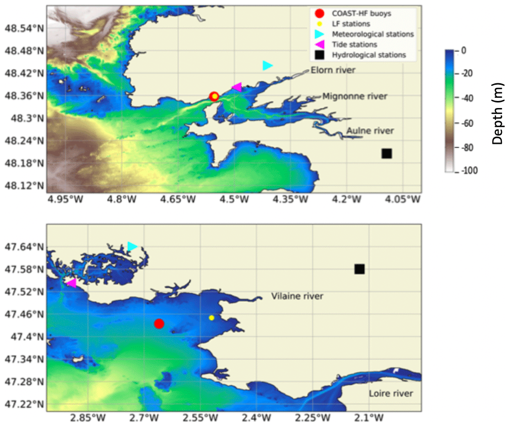
Figure 1 Location of the sampling sites: COAST-HF-Iroise and COAST-HF-Molit buoys (red circles); SOMLIT-Brest and REPHY-Loscolo sampling stations (yellow circles); Brest and Crouesty tide gauge stations (blue triangles); Guipavas and Vannes-Séné meteorological stations (purple triangles); hydrological stations of the Aulne and Vilaine rivers (black squares), with the Loire station off the map.

Sub-surface Chl a concentrations are provided by two French marine monitoring networks, the SOMLIT coastal observation network and the REPHY (French Observation and Monitoring programme for Phytoplankton and Hydrology in coastal waters).² Samples are collected bimonthly at the SOMLIT-Brest (48.358^∘ N, 4.552^∘ W) and the REPHY-Loscolo (47.496^∘ N, 2.445^∘ W) stations, which are close to the COAST-HF stations. Chl a concentrations are measured with either spectrophotometric or fluorimetric methods (Aminot and Kérouel, 2004).

Daily river flows are measured at gauging stations (French hydrology Banque Hydro database³), located close to the main river mouths (Aulne-Gouezec (48.205^∘ N, 4.093^∘ W), Loire-Montjean (47.106^∘ N, 1.78^∘ W)). The Vilaine River flow is controlled by a dam, and data are provided by the Vilaine Public Territorial Basin Organization (Fig. 1).⁴

The tide gauge stations (Shom⁵) at Brest (48.382^∘ N, 4.495^∘ W) and Crouesty (47.542^∘ N, 2.895^∘ W) record the sea level every minute.

Precipitation, air temperature, wind direction and intensity, and the solar flux data are retrieved every 6 min from two meteorological stations from the Météo-France observation network:⁶ Guipavas (48.440^∘ N, 4.410^∘ W) and Vannes-Séné (47.362^∘ N, 2.425^∘ W) (Fig. 1). We use the solar flux as a proxy for subsurface PAR (photosynthetically available radiation).

2.3 MARS3D-1DV modelling experiments

2.3.1 MARS3D-1DV model

A 1DV (one-dimensional vertical) model configuration is implemented to simulate changes in biogeochemical variables due to hydrodynamics and sediment dynamics in both bays.

The hydrodynamical model is based on the code developed for MARS3D (3D hydrodynamics Model for Applications at Regional Scale; Lazure and Dumas, 2008). This model is a primitive equation model with a free surface and uses the Boussinesq and hydrostatic pressure assumptions. We use the 1DV configuration of the model, with 10 vertical sigma levels for 15 m depth and a time step of 30 s.

The sediment model (MUSTANG – Le Hir et al., 2011; Grasso et al., 2015; Mengual et al., 2017) is designed to simulate the transport and changes in different sediment mixtures. In the sediment, 50 layers (refined near the surface) for a total thickness of 40 cm are implemented. Four sediment classes are considered: muds (diameter 10 µm), fine sand (diameter 100 µm), medium sand (diameter 200 µm), and coarse sand (diameter 400 µm). The sediment dynamics (transport in the water column, exchanges at the water–sediment interface, erosion/deposition processes) are driven by an advection/dispersion equation for each sediment class (refer to Le Hir et al., 2011, for a detailed description of the sediment model).

The biogeochemical model BLOOM (BiogeochemicaL cOastal Ocean Model) is derived from the ECO-MARS model (Cugier et al., 2005; Ménesguen et al., 2019) adding major processes of early diagenesis. Nitrogen, phosphorus, and silica cycles are studied considering four nutrients: nitrate, ammonium, soluble reactive phosphorus, and silicic acid (sorption/desorption of phosphate on suspended sediment and precipitation/dissolution of phosphate with iron processes are also included). The model is also represented by three phytoplankton classes (microphytoplankton, dinoflagellates, pico-nano-phytoplankton), two zooplankton classes (micro- and meso-zooplankton), and exchanges at the water–sediment interface and inside the sediment compartment.

2.3.2 MARS3D-1DV model sensitivity experiments

These three models (hydrodynamical, sediment, and biogeochemical) are coupled online during simulations and allow the nutrient and phytoplankton dynamics in both bays to be reproduced. The simulation for the Bay of Brest does not include nutrient inputs from the sediment because they are considered to be negligible around the COAST-HF-Iroise station.

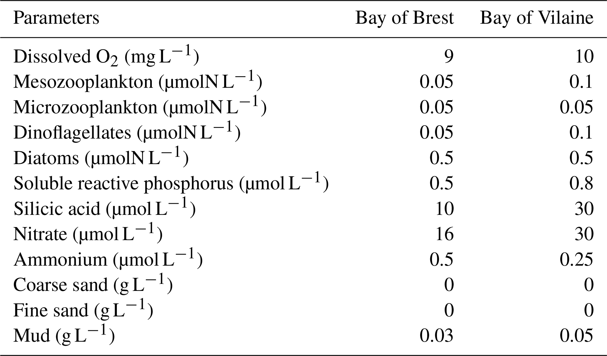
Dissolved and particulate variables are defined in the water column and in the sediment. Initial values for both bays are uniform over the initial vertical profile (Table 1) and are based on a 3D realistic coupled simulation during the year 2015. Values for the 15 February are extracted at the position of COAST-HF-Iroise for the Bay of Brest and at the position of the COAST-HF-Molit station for the Bay of Vilaine (Plus et al., 2021).

Table 1 Initial conditions in the water column for the MARS-1DV model for the beginning of the simulation on the 15 February.

To evaluate the sensitivity of the biogeochemical dynamics to environmental conditions, sensitivity experiments are then performed using the coupled MARS3D/BLOOM/MUSTANG 1DV model configuration. All simulations are started at the end of winter (15 February) and run until the end of the year. The range of values used in the sensitivity experiments are derived from the minimum and maximum observed in situ data. Each parameter is tested with a constant value for the whole simulation.

Three parameters are individually explored in both bays:

• The air temperature in sensitivity experiments ranges from 4 to 14 ^∘C and is controlled by the intensity of solar radiations. Air temperature represents the main controlling parameter of SST in the 1DV model. This parameter drives the radiative fluxes in the model and then constrains SST.

• Wind intensity effect on the IPGP is explored for values between 0 and 10 m s⁻¹. In the 1DV model, wind is a source of vertical mixing in the simulation.

• The cloud coverage (CC) sensitivity experiments ranged in value between 0 % CC and 100 % CC. This parameter is a driver of photosynthetic available radiation (PAR) in the ocean. For the formulation of radiative fluxes in the 1DV MARS3D model, 100 % cloud coverage allows an inflow of 38 % of the total solar radiation into the water column. Each individual experiment is associated with a constant CC applied to the seasonal solar radiation.

In the Bay of Vilaine, the sediment plays a role in light penetration and acts as an active source of nutrients: we therefore explored the influence of mud erosion rate (values between 2.10⁻⁵ and 2.10⁻⁷ kg m⁻² s⁻¹) in that bay (sand erosion rate fixed to 0.0001 kg m⁻² s⁻¹). For the sensitivity experiments, it drives a mass of sediment that is eroded and resuspended and a bottom input of nutrients in the water column.

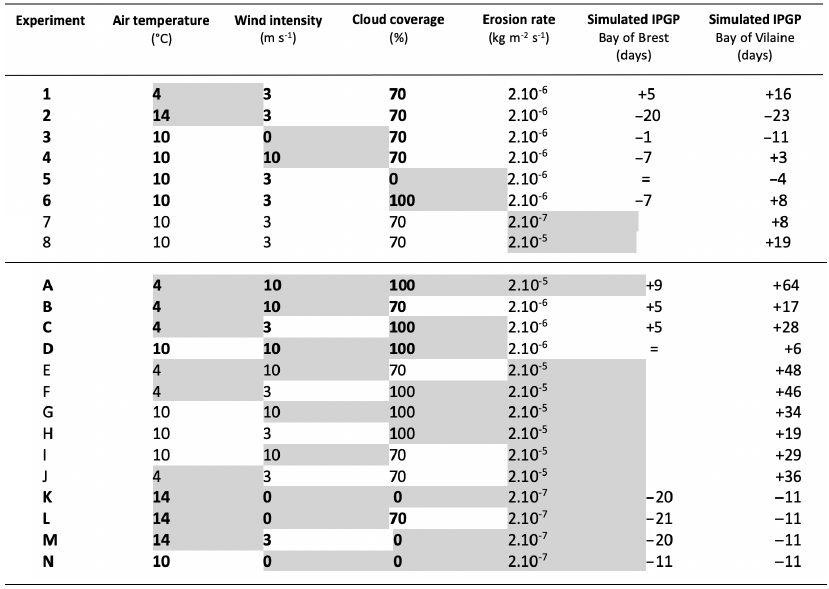
A second set of experiments is conducted by combining the individual effect of environmental parameters in order to explore possible cumulative or opposite effects on the IPGP. The upper and lower bounds of the range of environmental parameters are taken into account. Experiments are detailed in Table 5.

2.4 Data processing

2.4.1 Chl a fluorescence data

To analyse high-frequency time series of in situ Chl a fluorescence, the quenching effect (Lehmuskero et al., 2018) – a decrease in fluorescence in the presence of light (Fig. 2) – is removed by analysing only nighttime data, as reported in Carberry et al. (2019). Chl a fluorescence data are studied on a daily basis, i.e. averaged from 22:00 to 05:00. Years with less than 75 % of valid data are not considered in our analyses: for the Bay of Brest, these are the years 2005, 2006, 2008, 2009, and 2018.

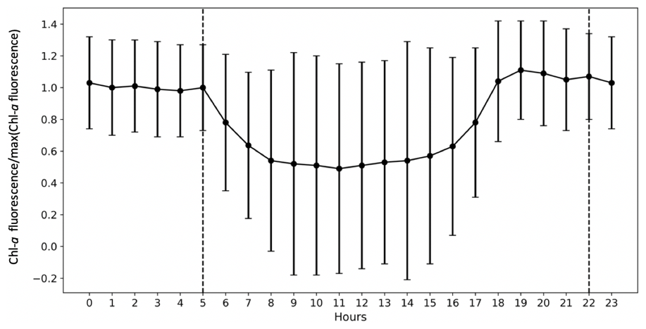
Figure 2 The importance of the quenching effect on Chl a fluorescence is represented by COAST-HF-Iroise data from 2000 to 2019. The standard deviation is represented by vertical black bars. The dashed lines represent the beginning and end of the selected values for the rest of the study from 22:00 to 05:00.

2.4.2 Detection of the IPGP

On the basis of the literature, we first apply three methods to determine the annual IPGP dates:

1. set an arbitrary beginning and end of the phytoplankton growing period at 20 % and 80 % of the cumulative Chl a fluorescence measured from 1 January to 31 December (Kromkamp et al., 2010),

2. consider a threshold of 5 % above the yearly median chlorophyll (Brody et al., 2013),

3. consider the beginning of the growing period as the maximum daily difference in Chl a fluorescence (Philippart et al., 2010).

Because none of these methods allowed us to obtain a valid IPGP detection – with too late (method 1) or too early (method 2) a detection or multiple IPGP dates (method 3) – we elaborate on a detection method based on discontinuities of the Chl a fluorescence signal (Fig. 3): daily FFU slopes are calculated based on a linear regression over a ± 2 d window for each day, from 1 January to 31 December, and each year. The IPGP date is identified when the slope exceeds a threshold value – defined as the median of the daily slopes – for the first time in the year for at least 20 d. The end of the phytoplankton growing period is determined when the slope stabilizes below the threshold for at least 20 d for the last time in the year. The cumulative Chl a fluorescence corresponds to the duration of the growing period.

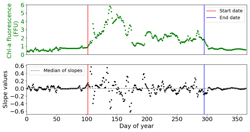
Figure 3 Example of detection of the start (red line) and end (blue line) of the phytoplankton growing period in 2001 at COAST-HF-Iroise. The threshold value – the median of slopes – is represented by a dotted grey line.

2.4.3 Pattern of the phytoplankton growing period

The k-means method (Hartigan and Wong, 1979) is used to characterize the annual patterns of the phytoplankton growing period.

We exclude the year 2013 from the analysis of the Bay of Vilaine because of a large number of missing data. When the interval over which consecutive data are missing is no longer than 1 week, we perform a linear interpolation to replace the missing data. A 5 d running average is applied to the Chl a fluorescence signal, and data are then normalized by the maximum value. We analyse Chl a fluorescence every year for 150 d after the IPGP.

Time series from both bays are merged before application of the k-means and the number of clusters (or centroids) is set to two to distinguish the dominant patterns of the phytoplankton growth period at both sites. The use of a larger number of clusters is investigated and does not produce a pattern representing a large number of observed growing periods.

2.4.4 Detection of extreme events

The peak over threshold method (see Oliver et al., 2018, and Poppeschi et al., 2021, for further details) is used to detect hydro-meteorological extreme events such as cold spells, flood events, and wind bursts. An event is regarded as extreme if values are higher than a given statistical threshold for at least 3 consecutive days. In the present study, the 90-percentile threshold is selected to detect floods and wind bursts, and the 10-percentile threshold is used to detect cold spells. Seasonal anomalies are calculated over at least 20 years, by subtracting raw data from the winter average value (for cold spells) or from the spring average value (wind bursts and floods).

3 Results

3.1 Characterization of the phytoplankton growing period

The high-frequency Chl a fluorescence time series at both sites show an intense seasonal cycle with low values from November to February and high values from March to October (Fig. 4). Focusing on the period from 2010 to 2019 in the Bay of Brest, the minimum Chl a fluorescence is observed during the years 2012 and 2013 and does not exceed 7 FFU. In contrast, some years show Chl a fluorescence values above 15 FFU but can be up to 20 FFU (such as 2010, 2014, 2015 or 2019). In the Bay of Vilaine, a similar seasonal pattern is observed with higher values reaching 50 FFU in 2013. Small (< 20 FFU) and high (> 35 FFU) Chl a fluorescence amplitudes are observed occasionally (in 2014 and 2017 and in 2013 and 2016, respectively). The Chl a fluorescence is higher, almost double, in the Bay of Vilaine compared to the Bay of Brest with a mean cumulative Chl a fluorescence of around 580 and 360 FFU, respectively (Table 2). The high phytoplankton biomass of the Bay of Vilaine is corroborated by the concentrations measured by low-frequency observation programmes (SOMLIT and REPHY).

Table 2 Global characteristics of the phytoplankton growing period in the Bay of Brest and in the Bay of Vilaine.

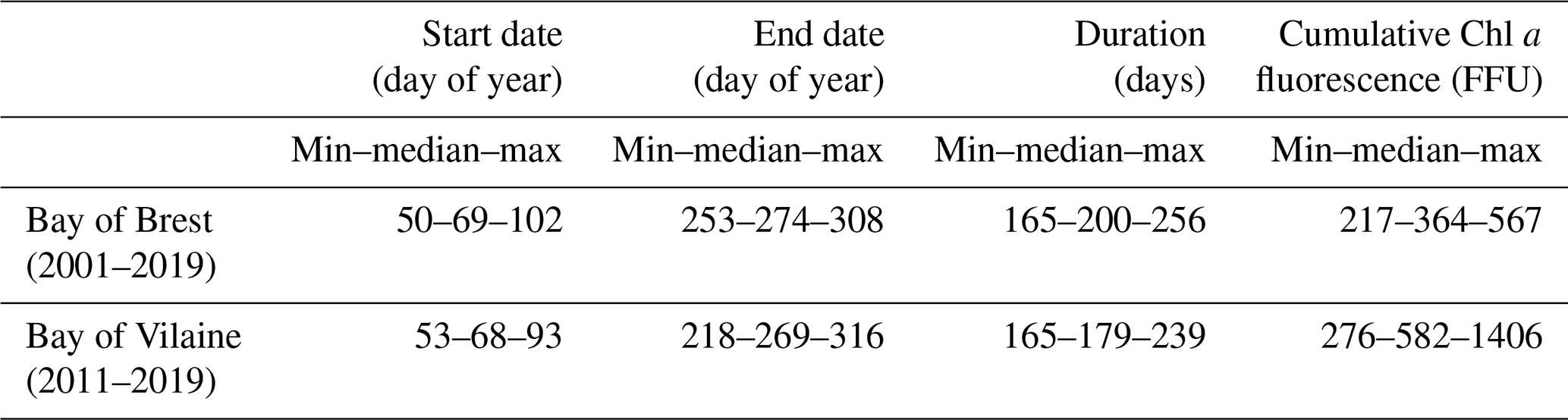
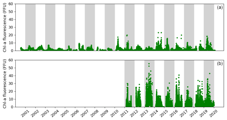
Figure 4 Temporal changes in the in situ Chl a fluorescence measured in the Bay of Brest (a) and the Bay of Vilaine (b).

The phytoplankton growing period ranges from approximately 10 March to 30 September in both regions (Table 2). The average duration of the phytoplankton growing period is 179 d in the Bay of Vilaine and 200 d in the Bay of Brest (Table 2). The phytoplankton growing period is characterized by successive blooms, whose number and intensity are variable from year to year (Fig. 4).

The main patterns of the phytoplankton growing period are identified by two clusters (Fig. 5). Cluster 0 includes the phytoplankton growing period with two successive marked blooms in early spring and in summer, the intensity of the second bloom being highly variable. Cluster 1 is characterized by a plateau during the first 2 months of the phytoplankton growing period. Most of the patterns of the Bay of Vilaine are in cluster 0, while those of the Bay of Brest are in cluster 1 (Table 3). The years that stand out in the Bay of Brest (2002, 2010, 2014) correspond to years with the highest cumulative Chl a fluorescence (≥ 450 FFU). The atypical years in the Bay of Vilaine (2011, 2017 and 2019) show the lowest cumulative Chl a fluorescence (≤ 450 FFU).

Table 3 Cluster group assigned to each annual phytoplankton growing period at both sites. The “–” dash represent years with missing data. The cross represents the year 2013 of the Bay of Vilaine, which was not considered.

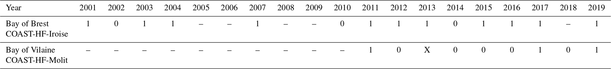
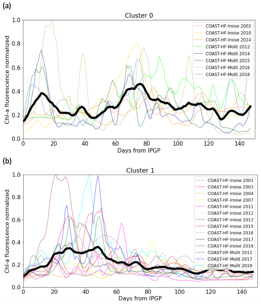
Figure 5 (a) Cluster 0 and (b) cluster 1 representative of the patterns of the phytoplankton growing period observed in both bays. The median pattern is drawn in bold.

3.2 Variability of the initiation of the phytoplankton growing period (IPGP)

Calculations performed to determine the IPGP for high- and low-frequency data yield comparable results (Fig. 6). The mean differences between the IPGP calculated with the high- and low-frequency data are 5 and 8 d for the Bay of Brest and the Bay of Vilaine, respectively. A difference of only 4 and 6 d between the model simulations (reference year: 2015) and the high-frequency in situ data are observed in the Bay of Brest and the Bay of Vilaine, respectively.

A decadal variability of the IPGP is recorded from mid-February to mid-April in both ecosystems (day 50 to day 102 in the Bay of Brest and day 53 to day 93 in the Bay of Vilaine; Fig. 6). In the Bay of Brest, early IPGPs (day < 53) are observed in 2010 and 2013, whereas late IPGPs (day > 93) are observed in 2001, 2017 and 2019. In the Bay of Vilaine, the earliest IPGP is detected in 2012 (day 53) and the latest in 2019 (day 93).

The variability of the IPGP in the Bay of Brest shows two linear trends (Fig. 6a), with a decrease of 52 d from 2001 to 2010 (observed in both high- and low-frequency datasets), followed by an increase (+48 d) from 2011 to 2019, a decline also observed in the Bay of Vilaine (Fig. 6b). Over the period 2011–2019, the IPGP is shifted towards a later date by +3.5 d per year in the Bay of Vilaine and +3.7 d per year in the Bay of Brest.

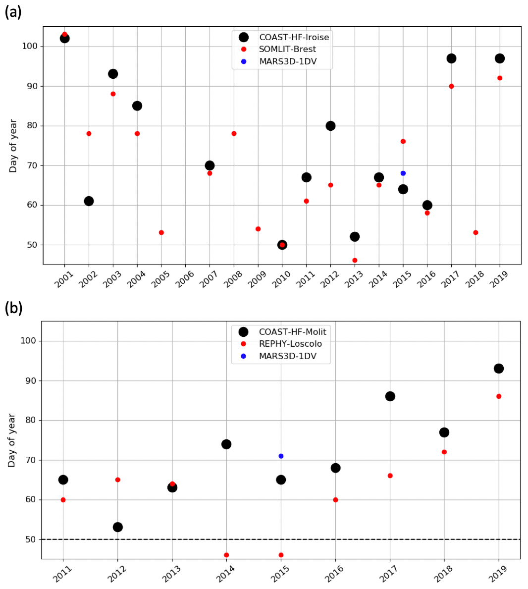
Figure 6 Changes in the IPGP date in (a) the Bay of Brest and (b) the Bay of Vilaine are determined with high-frequency time series (black circles), low-frequency time series (red circles), and with the model (blue circle). The dotted black line represents the date of the COAST-HF-Molit buoy deployment.

3.3 Analysis of environmental conditions driving the IPGP

3.3.1 Impact of environmental conditions on the IPGP

We next quantify the influence of environmental drivers on the date of the IPGP (Fig. 7). These drivers represent the major limiting factors of the phytoplankton growth and comprise input of nutrients (river flow), PAR (incident light), SST (air temperature, incident light), and turbidity in the water column (river flow, wind intensity, tidal range).

The median values of the environmental drivers observed at the date of each annual IPGP are very close in both bays (Table 4): temperate SST (10 ^∘C), weak wind (3 m s⁻¹), a medium PAR (1360 W m⁻²), a low turbidity (7 NTU), and a weak tidal amplitude (semi-amplitude of 1.6 m in the Bay of Brest and 0.9 m in the Bay of Vilaine). The IPGP occurs mainly during neap tides at 68 % in the Bay of Brest and 77 % in the Bay of Vilaine. The river flow is low during the IPGP with a runoff of 46 m³ s⁻¹ for the Aulne, 96 m³ s⁻¹ for the Vilaine, and 1196 m³ s⁻¹ for the Loire. These values are considered to be the favourable environmental conditions for this study.

Table 4 Characteristics of environmental drivers at the date of the IPGP except for nutrients from January to March in the Bay of Brest and in the Bay of Vilaine.

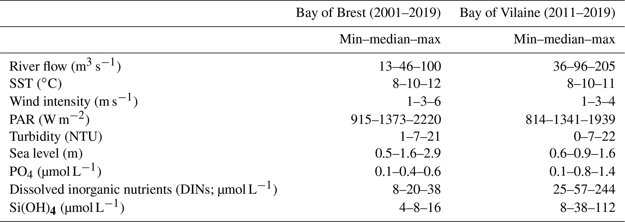
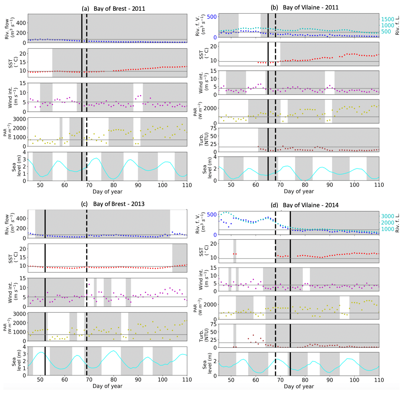
Figure 7 IPGP dates and environmental drivers: flow of the Aulne, Vilaine, and Loire rivers, sea surface temperature, wind intensity, PAR, turbidity, and sea level at high tide. Illustrations for a mean IPGP date in (a) the Bay of Brest and (b) the Bay of Vilaine in 2011; for an early IPGP date in (c) the Bay of Brest in 2013; for a late IPGP date in (d) the Bay of Vilaine in 2014. The mean IPGP date of each bay is represented by a dashed black line, and the IPGP date of the year is represented by a solid black line. Thresholds of each environmental driver are represented by grey horizontal lines corresponding to the mean conditions calculated 30 d around the IPGP date. Grey areas are time periods favourable to the IPGP.

To assess how environmental drivers may impact (i.e. advance or delay) the IPGP, we focus on the 15 d before the mean day of the IPGP (day 68) and of each annual IPGP. The considered 15 d length is related to the typical water residence time in both bays (Frère et al., 2017, and Poppeschi et al., 2021, for the Bay of Brest; Chapelle et al., 1994, and Ratmaya et al., 2019, for the Bay of Vilaine).

The earliest IPGP dates (IPGP < day 55) are associated with earlier occurrence of favourable environmental conditions than the other years. The earliest IPGP in 2010 and 2013 in the Bay of Brest and in 2012 in the Bay of Vilaine occurred before day 55 (Figs. 1f, 7c–2a). Early IPGPs between day 55 to 60, also associated with favourable environmental conditions, are found in 2002 and 2016 in the Bay of Brest (Fig. 1b, j).

The latest IPGP dates (IPGP > day 90) are associated with unfavourable environmental conditions until the date of the IPGP. The latest IPGPs occurring after day 90 are observed in 2001, 2003, 2017, and 2019 in the Bay of Brest and in 2019 in the Bay of Vilaine (Figs. S1a, c, k, l–S2g). For example, the delay detected in 2017 in both bays is due to strong wind and a lack of PAR until the day of the IPGP (Figs. S1k–S2e). Late IPGPs between day 70 to 90 are recorded in 2004, 2007, and 2012 in the Bay of Brest and in 2014, 2017, and 2018 in the Bay of Vilaine (Figs. S1d, e, g, 7d–2e, f).

The interannual variability of the date of the IPGP is therefore not controlled by a unique environmental driver. When the values of the environmental drivers responsible for the IPGP (Table 4) are compared to the mean values of the environmental drivers over a period of 30 d around the IPGP (Table S1), threshold values are observed in both bays: river flow is lower than usual (between 10 and 30 m³ s⁻¹), temperature is close to the expected value (10 ^∘C), wind is weak (0.5 to 1.5 m s⁻¹), PAR is stronger (> 300 W m⁻²), and turbidity is low (about 1.5 NTU). The IPGP starts around day 68 (± 3 d) on average (Fig. 7a, b).

3.3.2 Modelling the importance of the environmental drivers

The relative contribution of each environmental driver on the IPGP is determined by MARS-1DV simulations starting on 1 February (Fig. 8). Environmental drivers tested in the model control the following:

• sea temperature, explored in the model through air temperature (SST proxy),

• the level of water turbulence, through wind intensity,

• the available light, controlled by cloud coverage (CC, as a sea surface PAR proxy) and the erosion rate (turbidity proxy) limiting light penetration in the water column.

Model results show that early IPGPs are associated with an air temperature higher than 9 ^∘C (resulting in SST higher than 8 ^∘C), low wind intensity, weak CC, and low erosion rate. Environmental drivers responsible for early or late IPGPs are similar in both bays. Air temperature is the main driver with a potential deviation from the mean IPGP of 25 d in the Bay of Brest and 40 d in the Bay of Vilaine (Fig. 8). Wind, CC, and erosion rate have a lower impact on the IPGP (around 6 d in the Bay of Brest and 13 d in the Bay of Vilaine). In the Bay of Vilaine, the environmental drivers can simulate a later IPGP than in the Bay of Brest.

Figure 8 Impact of the variation in environmental drivers on the date of the IPGP in (a) the Bay of Brest and (b) the Bay of Vilaine. Steps of 1 ^∘C for the air temperature, 1 m s⁻¹ for the wind intensity, 10 % for the cloud coverage, and 0.0000036 kg m⁻² s⁻¹ for the erosion rate equivalent to a variation in suspended matter between 0.02 and 0.08 mg L⁻¹ at the IPGP.

In the Bay of Brest (Fig. 8a), only variations in air temperature have a real impact on the IPGP. If air temperature is low (< 8 ^∘C), the IPGP is not triggered before day 74 (Table 5, Exp 1). If air temperature is high (> 13 ^∘C), the IPGP can start on day 49 (Table 5, Exp 2).

Table 5 Assumptions are explored in the 1DV model for environmental parameters independently (1–8) and with a combined effect (A–N) with the modified values (grey background) and text in bold for the Bay of Brest only (+ for a later IPGP, − for an earlier IPGP, = for an equal IPGP) with the IPGP equal to the mean observed IPGP of day 68.

In the Bay of Vilaine, air temperature and the erosion rate are the two main drivers impacting the IPGP (Fig. 8b). As in the Bay of Brest, if air temperature is low (< 6 ^∘C), the IPGP is late and appears only after day 80 (Table 5, Exp 1). If temperature is equal or above 13 ^∘C, the IPGP is early and appears on day 45 (Table 5, Exp 2). If the erosion rate is low (2.10⁻⁷ kg m⁻² s⁻¹), the IPGP takes place on day 76 (Table 5, Exp 7). If the erosion rate is high (2.10⁻⁵ kg m⁻² s⁻¹), the IPGP occurs late after day 87 (Table 5, Exp 8).

Even if variations in wind and CC induce weaker shifts in the date of the IPGP, i.e. about 1 week at most (Table 5, Exp 3, 4, 5, 6), they can however explain some variations in the IPGP. For example, the fact that the early IPGPs, observed in 2010 in the Bay of Brest and in 2012 in the Bay of Vilaine, are due to low wind conditions (around 2 m s⁻¹, Figs. S2a–S1f) are confirmed by both in situ measurements and the model (Fig. 8b).

The combined effect of the environmental factors can also be explored from the MARS-1DV model simulations (Fig. 9). The modelling conditions (hereafter called “Exp”) are detailed in Table 5 and compared to the mean IPGP date (day 68).

The simulations confirm the observations: late IPGPs correspond to the most extreme unfavourable combined environmental values (temperature of 4 ^∘C, wind intensity of 10 m s⁻¹, CC of 100 %, and erosion rate of 2.10⁻⁵ kg m⁻² s⁻¹ – Exp A). Due to the most unfavourable conditions, the IPGP occurs 9 and 64 d later in the Bay of Brest and in the Bay of Vilaine, respectively. A late IPGP can also be linked to the combined effect of only two factors such as “temperature and wind” and “temperature and CC” with a delay of 5 and around 22 d, respectively (Exp B and C). In contrast, no delay is observed for the combination “wind and CC” (Exp D) in both bays.

Early IPGP events are found in the model simulations and in the in situ observations when conditions correspond to a high temperature (14 ^∘C), no wind intensity and CC, and a low erosion rate (2.10⁻⁷ kg m⁻² s⁻¹) – Exp K. All the combined scenarios allow the occurrence of an earlier IPGP (by at least 5 additional days) compared to experiments that consider a single modified parameter.

This analysis enables environmental parameters to be classified with respect to their impact on the IPGP. In both bays, the temperature appears to be the key factor driving the IPGP. By combining the environmental drivers, the IPGP can occur even later or earlier than with a single forcing. In both bays, the combination of wind and CC has no impact on the IPGP, which occurs near the median day (Exp D and N). The extreme couplings of Exp A, E, F, G, and J delay the date of the IPGP later than detected in the observations for the Bay of Vilaine. All simulations show a higher impact on the date of the IPGP in the Bay of Vilaine than in the Bay of Brest (Fig. 9, Table 5).

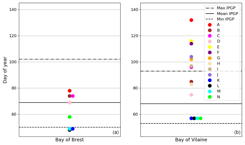
Figure 9 Influence of combined environmental parameters for the MARS-1DV model in both bays (Bay of Brest, a, and Bay of Vilaine, b) with detailed experiments in Table 2.

3.4 Impact of extreme hydro-meteorological events on the IPGP

3.4.1 Cold spells

The impact of cold spells on the IPGP is simulated with the MARS-1DV model based on two criteria: (i) the period of occurrence of the event, set in the middle or end of February; (ii) the duration and intensity of the cold spell, which can be either short and weak (8 d, 7 ^∘C) or long and intense (20 d, 5 ^∘C) (Fig. 10).

In both bays, when the cold spell appears in mid-February, the IPGP is not impacted. However, it is delayed by about 15 d when occurring at the end of February. The duration of the cold spell, when longer than 15 d, also has an impact on the IPGP, with a delay of 13 and 12 d in the Bay of Brest and in the Bay of Vilaine, respectively.

Eight cold spells are detected in February in both bays between 2001 and 2019. In 2011, both sites are impacted simultaneously with cold spells. Long cold spells (30 d) are observed in 2009 and 2018, leading to an anomaly of more than −1.9 ^∘C.

The cold spell observed in 2018 in the Bay of Vilaine may explain the later IPGP. There is no change in the IPGP in 2011 and 2013, despite the cold spell, the period of occurrence being too early during winter 2011 and the duration too short in 2013 (only 10 d).

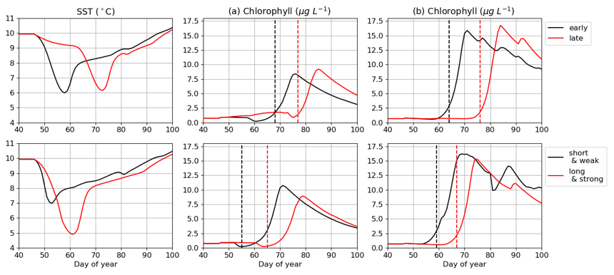
Figure 10 Impact of cold spells on the IPGP date simulated in (a) the Bay of Brest and (b) the Bay of Vilaine. Four conditions of cold spells are explored: early (mid-February), late (end of February), short (8 d), and long (20 d). The IPGP dates are represented by dashed lines.

In the Bay of Brest, the cold spells in 2003 and 2004 may explain the delay in the IPGP (respectively, days 93 and 85). The presence of long and intense cold spells in 2010 and 2011 does not shift the IPGP (days 50 and 67) because they occur too early (before day 20).

3.4.2 Wind bursts

Based on our model simulations, the wind bursts that occur during at least 3 continuous days have no impact on the IPGP in both bays, whatever the duration, the period, and the intensity (± 1 d). In the Bay of Vilaine, only one wind event is detected in 2018 (3 d long and 6 m s⁻¹). In the Bay of Brest, several events are detected, but no significant impact is observed on the IPGP.

3.4.3 Flood events

River floods can delay the IPGP by resuspending sediment in the water column and therefore limiting light penetration in the water column. Inputs of nutrients have no impact during the late winter period because nutrient concentrations are maximal, with no limitation on phytoplankton growth. Flood events are analysed with observation data collected in the month prior to the IPGP date because the 1DV modelling approach does not allow the sensitivity to hydrological events to be simulated (i.e. it is necessary to simulate horizontal advection processes).

In the Bay of Brest, the impact of flood events depends on their duration and intensity: when the flood exceeds 15 d, a delay in the IPGP is detected. Shorter and more intense floods (> 300 m³ s⁻¹) do not impact the IPGP.

In the Bay of Vilaine, only two flood events are observed close to the IPGP date in 2014 and 2015. The 2015 flood event, which is 10 d longer and more intense (> 100 m³ s⁻¹) than the 2014 one, delays the IPGP date by 10 d.

4 Discussion

4.1 Comparison of the phytoplankton growing period in both bays

Despite their contrasting hydrodynamics (e.g. Petton et al., 2020; Poppeschi et al., 2021; Lazure and Jegou, 1998; Ratmaya et al., 2019; Ménesguen et al., 2019), the median dates of the start and the end of the phytoplankton growing period are the same in the Bay of Brest and in the Bay of Vilaine, whether they are calculated from high- and low- frequency datasets or model simulations. The phytoplankton growing period occurs from March to September and lasts about 190 d in both bays. This concordance is related to a similar seasonality of the environmental drivers.

The observed cumulative fluorescence is almost double in the Bay of Vilaine compared with the Bay of Brest. This difference in the amount of chlorophyll produced in surface waters from both bays is also recorded by the low-frequency observation programmes and satellite observations (Ménesguen et al., 2019). It can be explained by the difference between the hydrodynamics and the influence of different watersheds. The Bay of Brest is a semi-enclosed bay with a macrotidal regime influenced by two local rivers (Aulne and Elorn), whereas the Bay of Vilaine has a weaker tidal regime, is open on the continental shelf and is widely influenced by a large river (Loire River).

Two different patterns of the phytoplankton growing period are identified by the k-means classification in both bays. The flattened, weak, and long bloom highlighted in the Bay of Brest can be explained by assuming that nutrients are not limiting the phytoplankton growth during spring. The maintenance of the diatom succession throughout spring since the 1980s (Quéguiner 1982; Del Amo et al., 1997) can be explained by the combination of increasing N and P loads, intense Si recycling and a macrotidal regime (Ragueneau et al., 2019). The phytoplankton growing period in the Bay of Vilaine is characterized by several successive peaks including two main ones. Nutrients drive the seasonal evolution of the phytoplankton growing period through periods of nutrient-limited conditions. These fluctuations are governed by phosphorus and nitrate loads from Vilaine and Loire rivers (Ratmaya et al., 2019) but probably also by the stoichiometry of recycled elements in the water and at the water–sediment interface (Ratmaya et al., 2022). At the beginning of the phytoplankton growing period (IPGP), however, the system is not nutrient-limited in terms of nitrate, phosphorus, and silicate (Table 4).

4.2 Validation of the method for IPGP detection

The method that we developed to detect the IPGP in both high-frequency and low-frequency in situ observations shows comparable results and detects similar initiation dates for some years, while a time lag between high- and low-frequency observations can be observed for other years. This difference is mainly explained by the difference in the sampling frequency. The late deployment of the buoy in the Bay of Vilaine (i.e. not deployed until mid-February before 2018) can also explain some differences between both sites. High-frequency data provide a more accurate detection of the day of the IPGP, while an uncertainty of about ± 7 d is observed with low-frequency observations. This comparison between high- and low-frequency-based IPGP detection highlights the sensitivity of sampling strategy in the observation of phytoplankton growing periods (Bouman et al., 2005; Serre-Fredj et al., 2021) related to the response of the ecosystem within a few hours after an environmental change (Lefort and Gasol, 2014; Thyssen et al., 2008).

The modelled IPGP, based on the year 2015, is coherent with high-frequency observations (around 5 d of difference between modelled and observed IPGP). Considering the idealized framework for modelling computations (1DV model instead of a realistic 3D model configuration), the agreement between observations and simulations validates the 1DV approach to explore IPGP dynamics. With the 1DV configuration, the vertical dynamics in the water column, coupled with biogeochemistry and sediment dynamics are reproduced well. Atmospheric forcings and interactions with the bottom layer are the main environmental drivers. The full range of impacts related to the horizontal advection (e.g. in the considered regions, river-advected plumes can change the hydrodynamics and the nutrient fluxes) are not evaluated, however. In the Bay of Brest and in the Bay of Vilaine, such advected sources exist (Poppeschi et al., 2021; Lazure and Jegou, 1998). But inputs from rivers are not the main drivers of the IPGP in nutrient-rich environments. Nutrient loads advected by rivers may impact the phytoplankton community later during the growing period rather than at the IPGP (Ratmaya et al., 2019).

4.3 Identification of the environmental conditions supporting the IPGP

The main theories to explain the initiation of phytoplankton blooms (Sverdrup, 1953; Huisman et al., 1999; Banse, 1994) are not relevant in the context of shallow and well-mixed coastal waters under the influence of river plumes. In the studied region, the ecosystem does not evolve with mixed layer dynamics, as observed in deeper environments. Both bays are permanently vertically mixed mainly by tides, and vertical stratification only occurs in a thin surface layer due to river runoffs at short timescales. However, the IPGP is mainly driven and limited by similar local environmental conditions in both bays. The ideal temperature (> 10 ^∘C) and PAR (1300 W m⁻²) for the IPGP are in agreement with those from previous studies conducted in similar coastal ecosystems (e.g. Glé et al., 2007; Townsend et al., 1994; Trombetta et al., 2019). Neap tidal conditions, weak wind (lower than 3 m s⁻¹), and weak river flow can also play a positive role in observations of earlier IPGPs according to previous studies (Ragueneau et al., 1996; Tian et al., 2011). The impact of wind direction on the IPGP is negligible.

Local changes in temperature, incident radiation, tidal conditions, wind conditions, and river flow induce differences in detected IPGPs. In this coastal temperate ecosystem, we observe that the beginning of the growing period is limited by light (controlled by incident radiation, turbidity in this season) and water temperature. The IPGP also occurs during low vertical mixing conditions.

The comparison of the individual importance of each environmental driver shows that temperature and light penetration are the key environmental drivers in both bays. When light penetration is reduced by a combined effect of PAR and turbidity (sediment resuspension), the delay in the IPGP can be amplified, especially in the Bay of Vilaine. The importance of light availability in the timing and intensity of the spring bloom is also highlighted in the North Sea (Wiltshire et al., 2015), in the German Bight (Tian et al., 2009), and along the UK south coast (Iriarte and Purdie, 2004).

4.4 Interannual evolutions of the IPGP

The IPGP in these two bays shows a strong interannual variability with initiation dates varying from late winter to spring, depending on the environmental conditions. A mean difference of 50 d between the earliest and latest IPGP dates is observed. It is important to note that the phytoplankton population during the IPGP is always dominated in both bays by the same centric diatoms, the genera Chaetoceros and Skeletonema, whose abundance varies from year to year depending on climatic conditions (REPHY, 2021). None of the nutrients limits the growing of phytoplankton at the IPGP (Table 4).

The earliest IPGPs are observed and related to favourable environmental conditions early in the year. For example, the IPGP can occur before day 50, associated with exceptionally weak wind and river flow in addition to a sufficient PAR and a near-optimal temperature of around 10 ^∘C (e.g. 2010 in the Bay of Brest and 2012 in the Bay of Vilaine). But if the environmental conditions are not favourable (e.g. 2017 and 2019 in both bays), the IPGP is delayed. This can be due to (1) strong wind for several days (not a single wind burst) combined with a weak PAR and sometimes enhanced by high-turbidity events which further limits the light penetration and (2) low SST.

The IPGP appears to be more controlled by local environmental drivers than by regional environmental drivers, the IPGP being earlier at one site than in the other during half of the studied years: for example, the 2012 IPGP is early in the Bay of Vilaine (day 53) but late in the Bay of Brest (day 80), related to strong wind activity and low PAR in the last bay. The offshore regional dynamics will induce limited impacts on local hydrodynamical features that will change the IPGP.

Changes in the IPGP over the last 2 decades have highlighted its evolution through two trends: it occurs earlier each year until 2010, when the trend is reversed. Changes in environmental conditions over the last 20 years were then studied to seek a possible concordance with one of the environmental drivers, but no significant trend was detected. Because of global warning, earlier phytoplankton blooms are expected (Friedland et al., 2018) but not a later IPGP as observed in our study regions. However, the mechanisms that trigger blooms in coastal ecosystems – especially eutrophic ones – are not similar to the processes that influence blooms in the open ocean. No link between trends in the IPGP and environmental drivers has been identified in the southern California Bight from 1983 to 2000 (Kim et al., 2009). By investigating long-term (1975–2005) daily data, Wiltshire et al. (2008) also observed later phytoplankton blooms in the German bight, but no link to global warming was detected. Henson et al. (2018) modelled a bloom shift of 5 d per decade from 2006 to 2025, with later blooms. A possible explanation of these later IPGPs may involve a lower spring SST (Hunter-Cervera et al., 2016).

4.5 Extreme events

We show that a cold spell is likely to delay the IPGP if it occurs at the end of winter (after 20 February) and/or if the cold spell lasts long enough (> 15 d). The drop in temperature related to the cold spell prevents the IPGP in both bays. This is in accordance with the study of Gomez and Souissi (2008) in the English Channel where cold spells can delay the date of the IPGP, as a result of an increase in water column mixing. Cold spells may also drive local patterns by influencing the phytoplankton communities (Gomez and Souissi, 2008; Schlegel et al., 2021).

Flood events have an influence on the phytoplankton biomass when they occur in spring, due to the supply of nutrients. When they occur in late winter, nutrients are already at their maximum. The impact of floods on the IPGP is then due to the increase in the water turbulence and to the limitation of light by increasing the turbidity. The IPGP can be delayed only if floods are at least 15 d long. This scheme was also observed by Saeck et al. (2013) along a river–estuary–bay continuum and explained by a shortened water residence time and limited light due to flood-induced turbidity in the coastal zone.

No relationship is observed between wind events and the IPGP in either bay because they are weakly stratified, contrary to open seas (i.e. Black Sea, Mikaelyan et al., 2017). In coastal stratified regions (e.g. under the influence of river plumes), strong wind and tidal mixing can enhance the mixing and break down stratification, which does not favour phytoplankton growth (Joordens et al., 2021). During the IPGP, except during floods, both regions are weakly stratified and are then less sensitive to combined wind/tidal short events.

5 Conclusions

This study provides a new understanding of the IPGP dynamics in coastal temperate areas by using both high- and low-frequency in situ data, in combination with simulations from a 1DV model. Strong similarities are found in both bays. An important interannual variability of the IPGP is observed, with a trend towards a later IPGP over the last decade (2010–2020). We quantify the importance of environmental conditions on the IPGP. When we compare observed IPGPs with favourable environmental conditions and following sensitivity experiments with the 1DV model, water temperature and turbidity (limiting light penetration in the water column) appear as the main drivers explaining interannual IPGP variability. The IPGP is a complex mechanism, usually triggered by more than one environmental parameter. The analysis of the influence of extreme events reveals that cold spells and floods have a strong impact by delaying the IPGP when episodes are long enough and occur after winter. No effect of wind bursts is detected.

While this study shows comparable IPGP dynamics when based on 1DV model simulations or in situ observations, we will next investigate the effect on phytoplankton dynamics of a fully realistic hydrodynamics (including horizontal and vertical advections; mixing processes; remote sources of nutrients from rivers) 3D model. We will focus on exploring the variability of phytoplankton communities during the IPGP to assess whether community change is occurring, as observed in other studies and for other ecosystems (Ianson et al., 2001; Edwards and Richardson, 2004; Chivers et al., 2020). When interannual evolutions in the phytoplankton growth are explored, the detection and the understanding of harmful algal bloom dynamics can also be addressed based on similar approaches. Further studies will be dedicated to the simulation of the coastal ecosystem in the future based on numerical simulation through climate scenarios. The investigation of other contrasting coastal environments will allow us to better understand and anticipate the expected impact of global change on coastal phytoplankton dynamics.