the Creative Commons Attribution 4.0 License.
the Creative Commons Attribution 4.0 License.
 | 16 Dec 2022
Evaluation of wetland CH4 in the Joint UK Land Environment Simulator (JULES) land surface model using satellite observations
Chris Wilson
Edward Comyn-Platt
Garry Hayman
Toby R. Marthews
A. Anthony Bloom
Mark F. Lunt
Nicola Gedney
Simon J. Dadson
Joe McNorton
Neil Humpage
Hartmut Boesch
Martyn P. Chipperfield
Paul I. Palmer
Dai Yamazaki
Wetlands are the largest natural source of methane. The ability to model the emissions of methane from natural wetlands accurately is critical to our understanding of the global methane budget and how it may change under future climate scenarios. The simulation of wetland methane emissions involves a complicated system of meteorological drivers coupled to hydrological and biogeochemical processes. The Joint UK Land Environment Simulator (JULES) is a process-based land surface model that underpins the UK Earth System Model (UKESM) and is capable of generating estimates of wetland methane emissions.
In this study, we use GOSAT satellite observations of atmospheric methane along with the TOMCAT global 3-D chemistry transport model to evaluate the performance of JULES in reproducing the seasonal cycle of methane over a wide range of tropical wetlands. By using an ensemble of JULES simulations with differing input data and process configurations, we investigate the relative importance of the meteorological driving data, the vegetation, the temperature dependency of wetland methane production and the wetland extent. We find that JULES typically performs well in replicating the observed methane seasonal cycle. We calculate correlation coefficients to the observed seasonal cycle of between 0.58 and 0.88 for most regions; however, the seasonal cycle amplitude is typically underestimated (by between 1.8 and 19.5 ppb). This level of performance is comparable to that typically provided by state-of-the-art data-driven wetland CH4 emission inventories. The meteorological driving data are found to be the most significant factor in determining the ensemble performance, with temperature dependency and vegetation having moderate effects. We find that neither wetland extent configuration outperforms the other, but this does lead to poor performance in some regions.
We focus in detail on three African wetland regions (Sudd, Southern Africa and Congo) where we find the performance of JULES to be poor and explore the reasons for this in detail. We find that neither wetland extent configuration used is sufficient in representing the wetland distribution in these regions (underestimating the wetland seasonal cycle amplitude by 11.1, 19.5 and 10.1 ppb respectively, with correlation coefficients of 0.23, 0.01 and 0.31). We employ the Catchment-based Macro-scale Floodplain (CaMa-Flood) model to explicitly represent river and floodplain water dynamics and find that these JULES-CaMa-Flood simulations are capable of providing a wetland extent that is more consistent with observations in this regions, highlighting this as an important area for future model development.
- Article
(13518 KB) - Full-text XML
- BibTeX
- EndNote


Methane (CH4) is a significant greenhouse gas, with a global warming potential (GWP) many times greater than that of CO2 (100-year GWP=28; Etminan et al., 2016). According to IPCC et al. (2021), methane accounts for approximately 20 % of the increase in radiative forcing from the pre-industrial period to the present day. The relatively short atmospheric lifetime of methane (∼9 years; Prather et al., 2012) means that reductions provide significant potential for mitigation of climate change to help address the goals of the Paris Agreement (O'Connor et al., 2010; Ganesan et al., 2019). However, the global methane budget is highly complex with a range of natural and anthropogenic sources (Saunois et al., 2020), many of which are still poorly constrained and possess large uncertainties (Dlugokencky et al., 2009; Nisbet et al., 2014).
Wetlands are the largest natural methane source and are comparable to (or larger in magnitude than) emissions from agriculture/waste and fossil fuels (Saunois et al., 2020). Natural wetlands are inundated ecosystems with water-saturated soil or peat and include permanent or seasonal floodplains, swamps, marshes and peatlands where the anaerobic conditions lead to CH4 production via methanogenic bacteria. Importantly, the uncertainty in CH4 emissions from wetlands remains one of the most significant challenges for understanding the global CH4 budget. Not only are there large uncertainties on processes and mechanisms related to the CH4 emission itself (Melton et al., 2013), but the wetland extent is highly uncertain (Bloom et al., 2010; Kirschke et al., 2013; Stocker et al., 2014) as is the response to meteorological drivers (Poulter et al., 2017; Parker et al., 2018).
One important step in better understanding the global CH4 budget is reconciling the bottom-up estimates of CH4 emissions (e.g. from land surface models) with top-down estimates based on atmospheric observations. The latest assessment of the global CH4 budget (Saunois et al., 2020) has a bottom-up estimate of wetland CH4 emissions of 149 Tg CH4 yr−1 (range of 102–182) compared with a top-down estimate of 181 Tg CH4 yr−1 (range of 159–200) for 2008–2017. Recent work (Folberth et al., 2022) has coupled wetland CH4 emissions from the Joint UK Land Environment Simulator (JULES) into the UK Earth System Model (UKESM) for the first time, allowing interactive wetland emissions from JULES to be used in climate simulations. To fully exploit this new capability, it is vital that the performance of the JULES wetland CH4 scheme is well-characterised and evaluated against present-day observations.
In this study, we perform an evaluation of the wetland CH4 emissions from the JULES land surface model using satellite observations of atmospheric CH4 columns in order to both assess the utility of the model in providing emission estimates as well as to diagnose any discrepancies against observations that may lead to future model improvements and increased understanding of the relevant processes.
The objectives of this study are as follows:
-
to provide an evaluation of the performance of JULES wetland CH4 simulations across the tropics using satellite remote sensing data;
-
to evaluate and characterise the differences in performance across an ensemble of JULES simulations with different configurations and identify the best-performing configuration(s) with the most suitable input data;
-
to explain the underlying reasons for poorly performing regions, relating these to the processes within JULES, and provide guidance on potential improvements.
In Sect. 2, we introduce the JULES land surface model, explain how wetland methane emissions are calculated and describe the ensemble of simulations that we have produced. Section 3 details the datasets and tools used to directly compare the JULES CH4 emissions to observations. In Sect. 4, we perform an evaluation of the seasonal cycle of JULES CH4 emissions over a range of wetland regions, and we focus in more detail on the challenging African regions in Sect. 5. We conclude the study in Sect. 6.
The Joint UK Land Environment Simulator, JULES (Best et al., 2011; Clark et al., 2011), is a process-based land surface model that both underpins the UK Earth System Model (Sellar et al., 2019) and acts as a stand-alone model capable of simulating many processes related to the land surface by describing the carbon, water and energy exchanges. We use JULES version 5.1 in this study.
2.1 Generation of wetlands within JULES
TOPMODEL (TOPography-based hydrological MODEL) is a rainfall–runoff model where estimates of surface and subsurface runoff are produced considering the topography of the land surface (Beven, 2012). This is defined through the topographic index, which is related to the relative propensity for soil saturation in that it incorporates both slope and upstream area. TOPMODEL was originally applied at the scale of small catchments, using pixels smaller than 50 m × 50 m in extent, but this framework has since been extended to global applications at a much wider range of spatial scales (Marthews et al., 2015; Gedney et al., 2019). TOPMODEL remains one of the most popular and widely used runoff production models (Beven et al., 2021) and has been implemented within the framework of the JULES model for many years (Best et al., 2011).
TOPMODEL is implemented in JULES as part of the large-scale hydrology scheme (Gedney and Cox, 2003; Best et al., 2011). A deep layer of restrictive water flow, added to the bottom of the standard soil column at a 3 m depth, results in the production of a saturated soil zone and a water table. The water table moves vertically when the soil moisture changes. Within each grid box the statistical distribution of topographic index (Marthews et al., 2015) is combined with the mean water table depth. This enables the simulation of a sub-grid water table distribution and, therefore, the extent of wetland in the grid box.
2.2 JULES wetland CH4 emissions
The JULES land surface model calculates methane wetland emissions () from three key factors, namely the amount of available substrate carbon, the temperature and the inundated area below the water table (Gedney et al., 2004; Clark et al., 2011):
is a dimensionless scaling constant () for wetland CH4 emissions when soil carbon is taken as the substrate for CH4 emissions. The wetland fraction (i.e. the proportion of a grid cell where the water table is at/above the surface and below a threshold indicative of significant flow; Gedney et al., 2004) is denoted by fw. z is the depth of soil column (in m), i is the soil carbon pool, κi (s−1) is the specific respiration rate of each pool (Table 8 of Clark et al., 2011), Cs (kg m−2) is soil carbon and Tsoil (K) is the soil temperature, averaged over the soil layers in the top 1 m of soil. The decay constant γ (=0.4 m−1) describes the reduced contribution of CH4 emission at deeper soil layers due to inhibited transport and increased oxidation through overlaying soil layers. This representation of inhibition is a simplification. However, previous work which explicitly represented these processes showed little to no improvement when compared with in situ observations (McNorton et al., 2016). We do not model CH4 emissions from freshwater lakes.
2.3 JULES ensemble experimental set-up
As outlined in Eq. (1), there are a variety of options within JULES and choices of input data that affect the calculation of CH4 from wetlands, which we call a “configuration”. In this study, we produce an ensemble of JULES simulations that spans a range of configurations. Different configurations allow adjustment of factors that have all been identified as key sources of uncertainty in previous wetland methane modelling efforts. We identify the optimal configuration(s) through comparison of model outputs against observations. The JULES ensemble that we produce comprises two different sets of meteorological driving data (ERA-Interim and WATCH Forcing Data ERA-Interim (WFDEI); Sect. 2.3.1), three different vegetation configurations (prescribed phenology and dynamic vegetation with and without competition; Sect. 2.3.2), two different temperature dependencies (Q10=3.7 and Q10=5.0; Sect. 2.3.3) and two different wetland extent parameterisations (the default from JULES and a version masked via the Surface WAter Microwave Product Series (SWAMPS) wetland extent; Sect. 2.3.4). This results in an ensemble with 24 members (). In order to identify ensemble members, we assign to each member a four-digit ID, as shown in Fig. 1. Thus the ensemble member using WFDEI meteorology data (2), using dynamic vegetation (3), with the lower temperature dependency (1) and with the original JULES wetland extent (1) is ensemble member 2311.
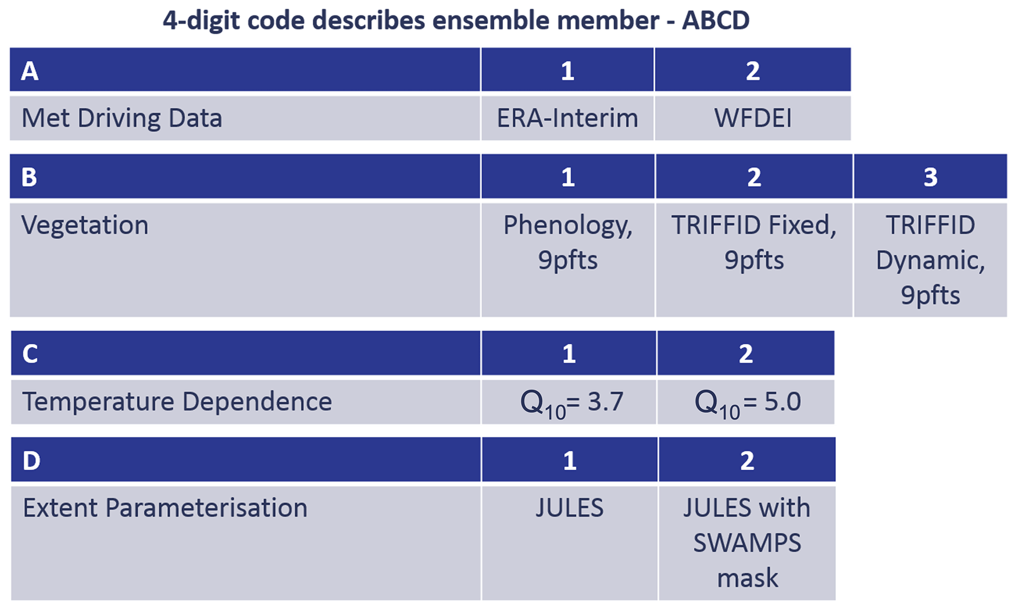
Figure 1Description of the 24 JULES ensemble members used in this study, comprising 2 meteorological driving data configurations, 3 vegetation configurations, 2 temperature dependencies and 2 wetland extent configurations. The four-digit code (ABCD) is used to identify the individual ensemble members.
In a post-processing step, the time series of annual wetland emissions of each ensemble member, regardless of whether they have been further constrained with a wetland mask or not, is separately scaled to give annual emissions of 180 Tg CH4 yr−1 for the year 2000 (Saunois et al., 2016), as described in Comyn-Platt et al. (2018). The scaling is most important when applied to the SWAMPS-based ensemble members as the geographic masking of the JULES wetland area with the SWAMPS data would otherwise result in reduced global emissions, below a level consistent with Saunois et al. (2016).
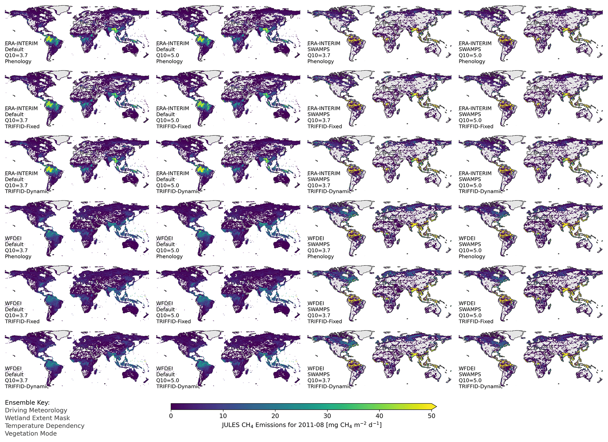
Figure 2Example (August 2011) of wetland CH4 emissions generated from each JULES ensemble members used in this study. The ensemble comprises two meteorological driving data configurations, two wetland extent configurations, two temperature dependency configurations and three vegetation configurations. Each panel is labelled with the details of its configuration, following the format of the key (shown in the bottom left).
Maps of the CH4 emissions for each ensemble member are presented in Fig. 2 for August 2011. Clear differences are observed relating to the different ensemble configurations, including the following: substantial differences between ERA-Interim and WFDEI-based ensemble members, with the magnitude of the emissions in the WFDEI members visibly smaller, and large spatial differences based on the default vs. SWAMPS wetland extent masking, with SWAMPS significantly reducing the wetland areas and concentrating the emissions, particularly removing the widespread but low emissions found more generally in the default members.
2.3.1 Driving data: ERA-Interim vs. WFDEI
Meteorological forcing data are used to drive the JULES land surface model. The meteorological parameters used in this study are as follows: air temperature, surface pressure, precipitation, short- and long-wave radiation, relative humidity, and wind speed. In the ensemble, we use two sources for the meteorological data: ERA-Interim and WFDEI.
The ERA-Interim reanalysis (Dee et al., 2011) is a widely used global atmospheric reanalysis product produced by the European Centre for Medium-Range Weather Forecasts (ECMWF). WFDEI is based on the ERA-Interim reanalysis data but includes the modifications as outlined in Weedon et al. (2014). These include interpolation to a resolution, a sequential elevation correction and a monthly bias correction based on observations.
2.3.2 Vegetation
Vegetation is represented by nine plant functional types (PFTs): broadleaf deciduous trees, tropical broadleaf evergreen trees, temperate broadleaf evergreen trees, needle-leaf deciduous trees, needle-leaf evergreen trees, C3 and C4 grasses, and deciduous and evergreen shrubs (Harper et al., 2016). Depending on the options chosen, these PFTs can be in competition for space, based on the TRIFFID (Top-down Representation of Interactive Foliage and Flora Including Dynamics) dynamic vegetation module within JULES (Clark et al., 2011). There are also four non-vegetated surface types: urban, water, bare soil and ice.
The ensemble uses three different JULES configurations to describe the vegetation behaviour (Clark et al., 2011): a configuration based on calculating leaf-level phenology and two configurations based on the TRIFFID dynamic vegetation module in JULES, with and without vegetation competition (i.e. allowing for changes in surface coverage by different PFTs or not respectively). The calculation of leaf phenology is independent of the calculation of the evolution of vegetation coverage and is available even when the TRIFFID dynamic vegetation module is not used.
The number of carbon pools used in Eq. (1) depends on the soil biogeochemistry model (soil_bgc_model) and vegetation options selected. For the leaf phenology vegetation option, soil_bgc_model = 1 and a single (fixed) soil carbon pool is used. For the vegetation configurations using the TRIFFID dynamic vegetation model, soil_bgc_model = 2 and four carbon pools are used based on the RothC model (Clark et al., 2011).
2.3.3 Temperature dependence: Q10=3.7 vs. 5.0
As indicated in Eq. (1), the CH4 emission is strongly dependent on the temperature of the soil. This temperature dependency of methanogenesis is generally parameterised using a Q10 value that approximates the Arrhenius equation. As discussed in Gedney et al. (2004), the approach that JULES takes due to applying this approximation globally over a wide temperature range is to use an effective or generalised Q10 that fits the form of the Arrhenius equation exactly (Eq. 2).
We chose Q10 values of 3.7 and 5 based on the work of Gedney et al. (2019), who tested respective values of 3, 3.7 and 4.7 as low, middle and upper estimates based on Turetsky et al. (2014) values for poor fens, rich fens and bogs.
2.3.4 Wetland extent: JULES vs. JULES with SWAMPS mask
JULES generates wetland extent following the TOPMODEL approach, as outlined in Sect. 2.1. As accurate wetland extent is one of the largest challenges in relation to modelling wetland emissions of methane (Saunois et al., 2020), the ensemble also provides an alternative observationally constrained wetland extent. In this instance, the JULES wetland area is simply masked by the SWAMPS dataset (Schroeder et al., 2015), meaning that any wetland extent that is inconsistent with the SWAMPS observations is disregarded.
3.1 GOSAT CH4 observations
The primary observational dataset that we use for evaluation of the JULES CH4 is the University of Leicester GOSAT Proxy XCH4 (Parker et al., 2011, 2020a). The GOSAT satellite, launched in 2009 by the Japanese Space Agency, was the first dedicated greenhouse gas observing satellite (Kuze et al., 2009). These data were recently used (Parker et al., 2020b) to evaluate the WetCHARTs CH4 emission database (Bloom et al., 2017a) and have previously been used for many wetland-related studies, including Parker et al. (2015), Berchet et al. (2015), McNorton et al. (2016), Lunt et al. (2019), Saunois et al. (2020), Wilson et al. (2021), Maasakkers et al. (2021) and Lunt et al. (2021).
GOSAT measures the signal of reflected sunlight in the short-wave infrared (SWIR) and, as such, is capable of providing measurements over land and also over the ocean in cases where sun-glint reflection allows. The GOSAT Proxy XCH4 retrieval provides around 15 000–25 000 observations over land each month and, after changes to the sun-glint sampling in 2015, a comparable number over the ocean. For a full description of the data, including evaluation and validation, see Parker et al. (2020a).
3.2 TOMCAT atmospheric CH4 simulations
In order to link surface CH4 emissions as generated by JULES with atmospheric observations as measured by GOSAT, it is necessary to run the emissions through a global chemistry transport model.
In this study, we use the TOMCAT 3-D model (Chipperfield, 2006), run globally between 2009 and 2017 at a 1.125∘ horizontal resolution and 60 vertical levels up to 0.1 hPa. The model set-up is consistent with that in Parker et al. (2020b). In short, non-wetland CH4 fluxes are taken from the Emissions Database for Global Atmospheric Research (EDGAR) v4.2 database for anthropogenic emissions and the Global Fire Emissions Database (GFED) v4.1s dataset for biomass burning emissions. Annually repeating rice paddy emissions are used from Yan et al. (2009), with ocean and termite sources used following Patra et al. (2011). The atmospheric (OH, O(1D) and stratospheric Cl) and soil sinks are as described in McNorton et al. (2016).
For the wetland CH4 fluxes, the emissions generated for each of the 24 JULES ensemble members (Sect. 2.3) are assigned to individual tracers. These tracers each contain the wetland and non-wetland CH4 fluxes; therefore, an additional tracer containing no wetland emissions is used as a reference to remove the non-wetland effects.
The model was initialised using the same method as Parker et al. (2018) and Parker et al. (2020b), which, in turn, were based on simulations from McNorton et al. (2016). The model tracers were initialised in 1977 and ran up to 2004 at a coarser resolution (2.8∘) than the main simulation. At this point, the tracers were scaled to match the overall observed surface concentration for CH4. The period from 2004 to 2009 was then run at the 1.125∘ resolution before the analysis began in 2009.
In this section, we evaluate the seasonal cycle of the wetland CH4 emissions generated from the ensemble of JULES simulations against atmospheric satellite observations. We perform the same analysis on the JULES wetland emission datasets as was used for the evaluation of the WetCHARTs emission dataset (Parker et al., 2020b), thereby enabling comparison of results and conclusions.
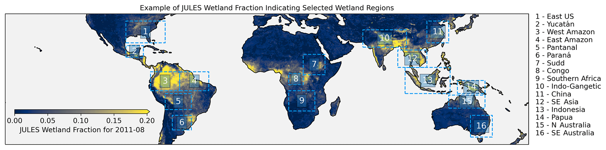
Figure 3Map showing the locations of the 16 wetland regions considered in this study. A representative month (August 2011) of the JULES wetland fraction is shown as the basemap.
The evaluation is performed over 7 large-scale areas (global, Northern Hemisphere, Southern Hemisphere, 60∘ S–60∘ N, tropics, north tropics and south tropics) as well as 16 specific wetland areas, as indicated in Fig. 3.
To calculate the XCH4 seasonal cycle, we apply the NOAA curve-fitting routine (ccgcrv) (Thoning et al., 1989; NOAA, 2022) to the GOSAT CH4 observations as well as the TOMCAT model simulations for each of the JULES wetland emission ensemble members. To determine the wetland-specific signal, we apply the same technique to the TOMCAT tracer that contained no wetland emissions and subtract that signal. This method does make the assumption that the uncertainties in the inter-annual variability in non-wetland XCH4 sources (such as biomass burning) are much smaller than the uncertainty in wetland methane emissions. This assumption has previously been tested (e.g. Parker et al., 2020b; Wilson et al., 2021), and inversion results suggest that, whilst it is possible for fire emissions to interfere with our analysis to a small degree, this is largely not the case with flux changes in fire-affected regions generally remaining consistent with the prior (see Appendix B for more details). In future work, CO inversions, currently under development, will allow us to better represent the XCH4 flux from biomass burning and separate any effect more explicitly.
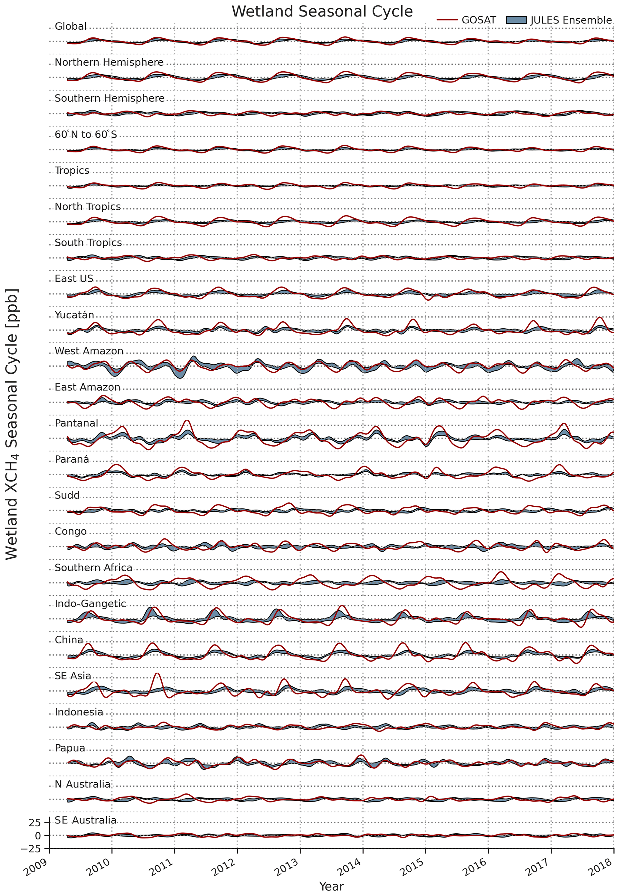
Figure 4Time series showing the GOSAT (red) and JULES ensemble (blue, min/max envelope) wetland CH4 seasonal cycles (in ppb) for 7 large-scale areas and 16 specific wetland regions. The wetland seasonal cycle is calculated by subtracting the TOMCAT model simulations that do not contain any wetland emissions. For each time series, the dashed horizontal lines indicate the [−25, 0, 25] levels, as indicated in the bottom panel.
The above method results in a wetland XCH4 seasonal cycle for each region from GOSAT and from each of the model ensemble members (Fig. 4). The observed (GOSAT) seasonal cycle magnitude varies significantly between regions (e.g. contrast the Pantanal and East Amazon regions) and can also be seen to vary strongly between years for the same region (e.g. contrast SE Asia for the period from 2010 to 2017). Qualitatively, the ensemble of JULES-based simulations are not dissimilar to the observations; however, the simulated seasonal cycles are typically weaker in magnitude than the observations. Although the ensemble spread can be large in some regions (e.g. Indo-Gangetic region), the areas with a strong observed seasonal cycle typically exhibit a strong seasonal cycle in the JULES ensemble, albeit typically with a smaller magnitude. This suggests, overall, that JULES is generally capable of reproducing the region-to-region and month-to-month wetland emissions that we see from observations, but details for specific regions can fail to match the observations.
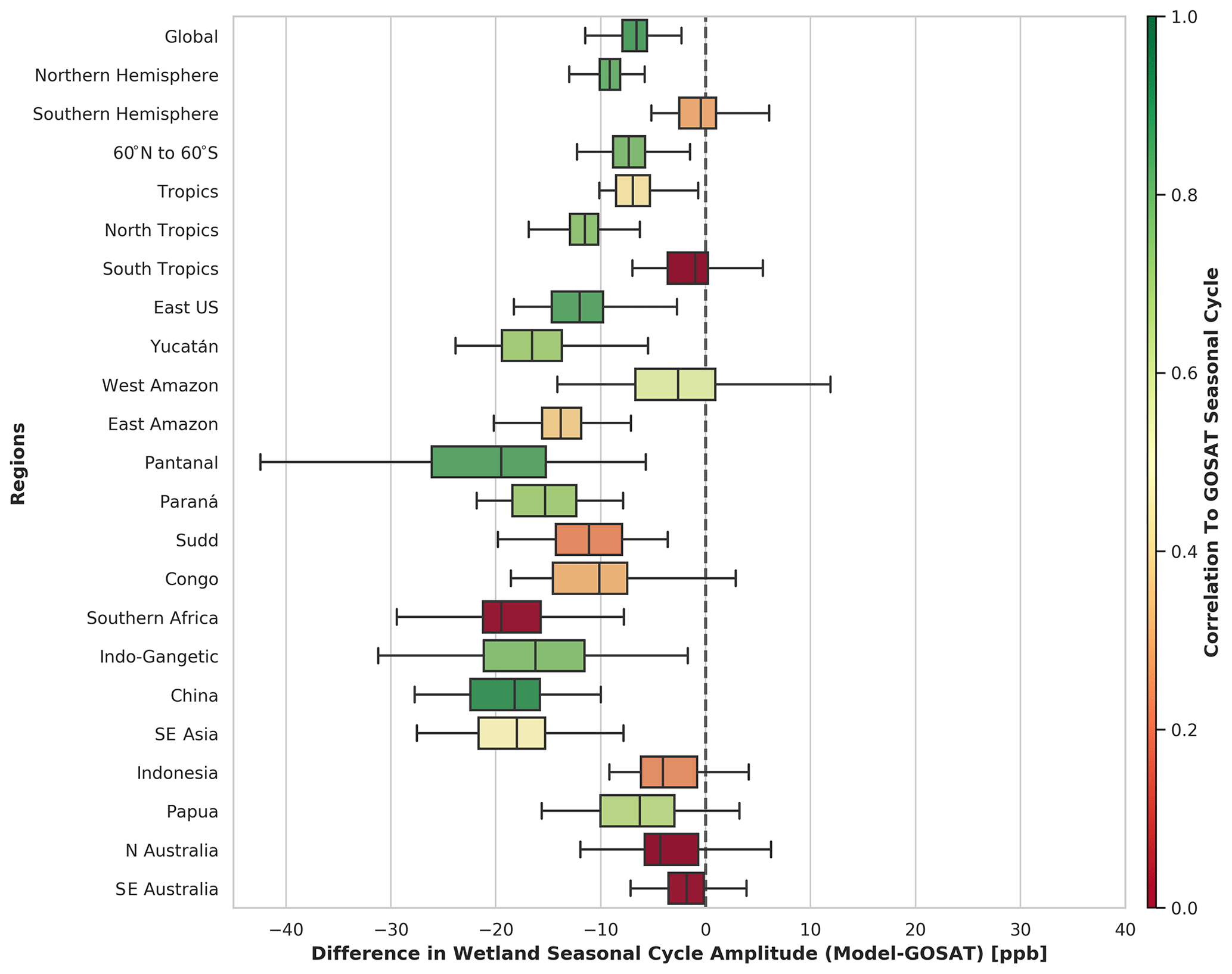
Figure 5Box plot showing the distribution of the difference in the wetland CH4 seasonal cycle amplitude between the JULES ensemble and GOSAT observations for all years (2009–2017). A box-and-whisker (box: quartiles; whiskers: min/max) plot is calculated for each of the regions (7 large-scale areas and 16 specific wetland areas) and is coloured by the mean value of the correlation coefficient between the modelled and observed wetland CH4 seasonal cycle.
A more rigorous quantitative evaluation of the seasonal cycle phase and magnitude is shown in Fig. 5. In this analysis, we produce a box-and-whisker plot for the distribution of the model–GOSAT wetland XCH4 seasonal cycle amplitude differences (ΔA), combining all ensemble members and all years for each region. Further, the box is coloured according to the mean value of the correlation coefficient (Rcycle) between the GOSAT and model seasonal cycles. In this way, we attempt to portray two separate aspects of the model performance. The box-and-whisker plot indicates the difference in the amplitude of the seasonal cycle for each year, while the colours indicate the correlation coefficient of the time series. It is entirely possible to have highly correlated time series where the amplitude of the signal is different (e.g. two perfectly in sync seasonal cycles but one with a very different amplitude to the other). This is the case for regions such as the Pantanal, where the seasonality between JULES and GOSAT matches well but the amplitude of the seasonal cycle is much larger in GOSAT than JULES (see the Pantanal panel in Fig. 4). Conversely, there are regions where the maximum amplitude difference is small but the seasonally cycles are out of phase, leading to a poor correlation (e.g. see the Indonesia panel in Fig. 4).
The lower limit of the colour scale in Fig. 5 is capped at zero, although it should be noted that one region (N Australia) has a negative correlation of −0.16. However, the seasonal cycle over this region is very small (<5 ppb); hence, the correlation is not particularly meaningful.
Globally we find that the JULES ensembles underestimate the XCH4 wetland seasonal cycle amplitude by approximately 6.6 ppb (quartiles: 5.6–7.9 ppb) with a correlation coefficient of 0.85. When considering the Northern and Southern hemispheres, we see somewhat different behaviour: ΔA of −9.2 and −0.4 ppb respectively. This north–south difference is exaggerated further when contrasting the north tropics ( ppb, Rcycle=0.73) and the south tropics ( ppb, Rcycle=0.0).
When focusing on specific wetland regions, we find that the evaluation is varied and performance is very dependent on the region. For example, although Rcycle=0.83 for the Pantanal region, suggesting that the phase of the seasonal cycle is reasonably well-captured, the seasonal cycle amplitude is significantly underestimated ( ppb); furthermore, this underestimation has a very large spread between ensemble members and years (ranging from −42.4 to −5.7 ppb). In contrast, the Paraná region has a slightly poorer Rcycle (0.70) and slightly better ΔA (−15.3 ppb) but with significantly smaller spread between ensemble members (−21.8 to −7.9 ppb).
For the majority of wetland regions (East US, Yucatán, West Amazon, Pantanal, Paraná, Indo-Gangetic, China and Papua), Rcycle shows a reasonable correlation of between 0.58 and 0.88. However, several regions stand out as having a particularly poor Rcycle value (East Amazon, Sudd, Congo, Southern Africa, Indonesia, N Australia and SE Australia). This poor correlation coefficient is easily explained for some regions (especially the Australian regions) where the seasonal cycle itself is very small (Fig. 4). However, of particular note are the three African regions (Sudd, Congo and Southern Africa) where the seasonal cycle itself can be relatively strong but timing is in poor agreement between the JULES ensemble and the observations (Rcycle values of 0.23, 0.31 and 0.01 respectively). We revisit these regions in Sect. 5 and perform a more detailed evaluation in order to explain the poor performance here.
Despite these few poorly performing regions, JULES shows reasonable to good performance overall in representing the observed seasonal cycle. It is informative here to judge the performance of JULES against the current state-of-the-art wetland emission dataset, WetCHARTs. In Parker et al. (2020b), we evaluated the performance of WetCHARTs in the same way as we evaluate JULES here, so a direct comparison of the ability to model the observed seasonal cycle can be made. We reproduce Fig. 4 from Parker et al. (2020b) in the Appendix of this work (Fig. A1) and contrast it against Fig. 5 from this study. Overall the comparisons for the different wetland regions are largely in agreement, with a strikingly similar distribution in ΔA between regions. Both WetCHARTs and JULES typically underestimate the wetland seasonal cycle magnitude, with the largest ΔA occurring in the same regions (Southern Africa, Indo-Gangetic, China and SE Asia). The largest discrepancies between the JULES analysis and our previous WetCHARTs analysis are as follows: for WetCHARTs, the ensemble spread (σA) in the Congo is far larger than for JULES, while Rcycle is reasonable compared to poor for JULES; although the biases for Southern Africa are very similar, Rcycle for WetCHARTs is reasonable, while again, it is poor for JULES. The above findings suggest that the performance of JULES is very comparable to that of the observation-driven WetCHARTs emissions, albeit with some differences in key regions.

Figure 6The change in correlation coefficient (top) and standard deviation (bottom) between the JULES ensemble and GOSAT wetland CH4 seasonal cycle when controlling for the remaining ensemble parameters. The change is the difference above the minimum value for each set of ensemble members. An increased correlation coefficient should be considered an improvement, whereas an increased standard deviation should be considered a deterioration. The changes are calculated for all 16 wetland regions in this study and presented as a box-and-whisker plot (box: quartiles; whiskers: min/max).
4.1 Attribution of performance to specific configuration choices
A significant feature apparent in the analysis so far is that the spread in ΔA across the ensemble members is typically large, often in excess of 20 ppb between the minimum and maximum ΔA values. Understanding which ensemble members perform well (and poorly) is an important step towards identifying which parameters and processes are driving the discrepancies to observations. To investigate this, we calculate the change in two metrics: the correlation coefficient between the GOSAT and modelled wetland seasonal cycle (Rcycle) and the standard deviation of the seasonal cycle amplitude (σA), above the minimum value for that metric. We denote these respective changes as ΔRcycle and ΔσA. We do this for the different ensemble parameter groupings (meteorological driving data, vegetation, temperature dependency and wetland extent) individually and hold the other parameters constant. To elaborate, out of the 24 ensemble members, the ensemble is split into () groupings (see Sect. 2.3 and Fig. 1). Using the meteorological driving data as an example, there are 12 different configurations that use ERA-Interim and 12 configurations that use WFDEI. We compare the statistics for the performance of these configurations for pairs of configurations where the only difference is which meteorological driving data are used and calculate the change in the metric between the highest and lowest values. We then do likewise for the other parameters (vegetation, temperature dependency and wetland extent). Note that there are three configuration possibilities for vegetation (phenology, fixed-TRIFFID and dynamic-TRIFFID), and this results in triplets rather than pairs of members that are compared. For clarity, the values that we report are the change above the minimum value for each pair/triplet; hence, by construction, this is a positive (or zero) value.
The results of this analysis are presented in Fig. 6 with all regions collated into a single set of results. The ensemble members driven by WFDEI consistently outperform the ERA-Interim-based members, with both a significantly higher ΔRcycle (a median increase of 0.12 with quartile values of 0.02 and 0.24) and significantly lower ΔσA (a median decrease of 0.53 ppb). For the vegetation configurations, the results are more mixed, without any single configuration being substantially better than the rest, but the phenology-based configurations do exhibit a slightly higher ΔRcycle value (0.03, 0.01 and 0.01 for phenology, TRIFFID-Fixed and TRIFFID-Dynamic respectively) and lower ΔσA value than the TRIFFID configurations, suggesting that they perform slightly better overall. However, the significant overlapping spread here suggests that these results are much more dependent on the region. For temperature dependency, the lower Q10 value (3.7) performs better than the higher Q10 value (5.0), but, again, the spread in both ΔRcycle (e.g. 75th percentile values of 0.15 and 0.09 for a Q10 of 3.7 and 5.0 respectively) and ΔσA (75th percentile values of 0.53 and 0.72 ppb respectively) are high, suggesting a large region-to-region variability (consistent with Turetsky et al., 2014, who measured a wide range of Q10 values across different wetland types). Finally, the choice of wetland extent between JULES and SWAMPS is found to make little difference, with SWAMPS very slightly increasing the correlation and decreasing the standard deviation over the original JULES. We discuss this aspect in more detail below.
Overall, we can conclude that the source of the meteorological driving data (ERA-Interim vs. WFDEI) is the most significant factor in how well JULES is able to reproduce the wetland seasonal cycle, with WFDEI performing (almost) unanimously better than ERA-Interim over the 16 wetland regions that we consider. In this context, an important factor is that WFDEI precipitation is bias-corrected using the observed monthly mean (Weedon et al., 2014). This is likely the cause of the significant improvement in wetland extent obtained by using WFDEI over ERA-Interim. The choice of the vegetation and temperature dependency configurations were found to improve (or worsen) the representation of the seasonal cycle depending on their choice, but this was found to be much more region-dependent with a greater spread. Perhaps surprisingly, the choice of wetland extent configuration was found to have less of an effect when collating results across all regions. However, an important point to make here is that we are solely comparing the performance between two extent configurations, and we find that neither is significantly better than the other. This does not preclude extent itself from being important. It should also be remembered here that, for the majority of regions, Rcycle already shows a good correlation to observations for the majority of ensemble members (see Fig. 5), implying that the extent is already sufficiently well-reproduced in these regions. In the following section, we focus on case studies over the three poorly performing African wetland regions and demonstrate the significance of poorly reproducing the wetland extent in these regions.
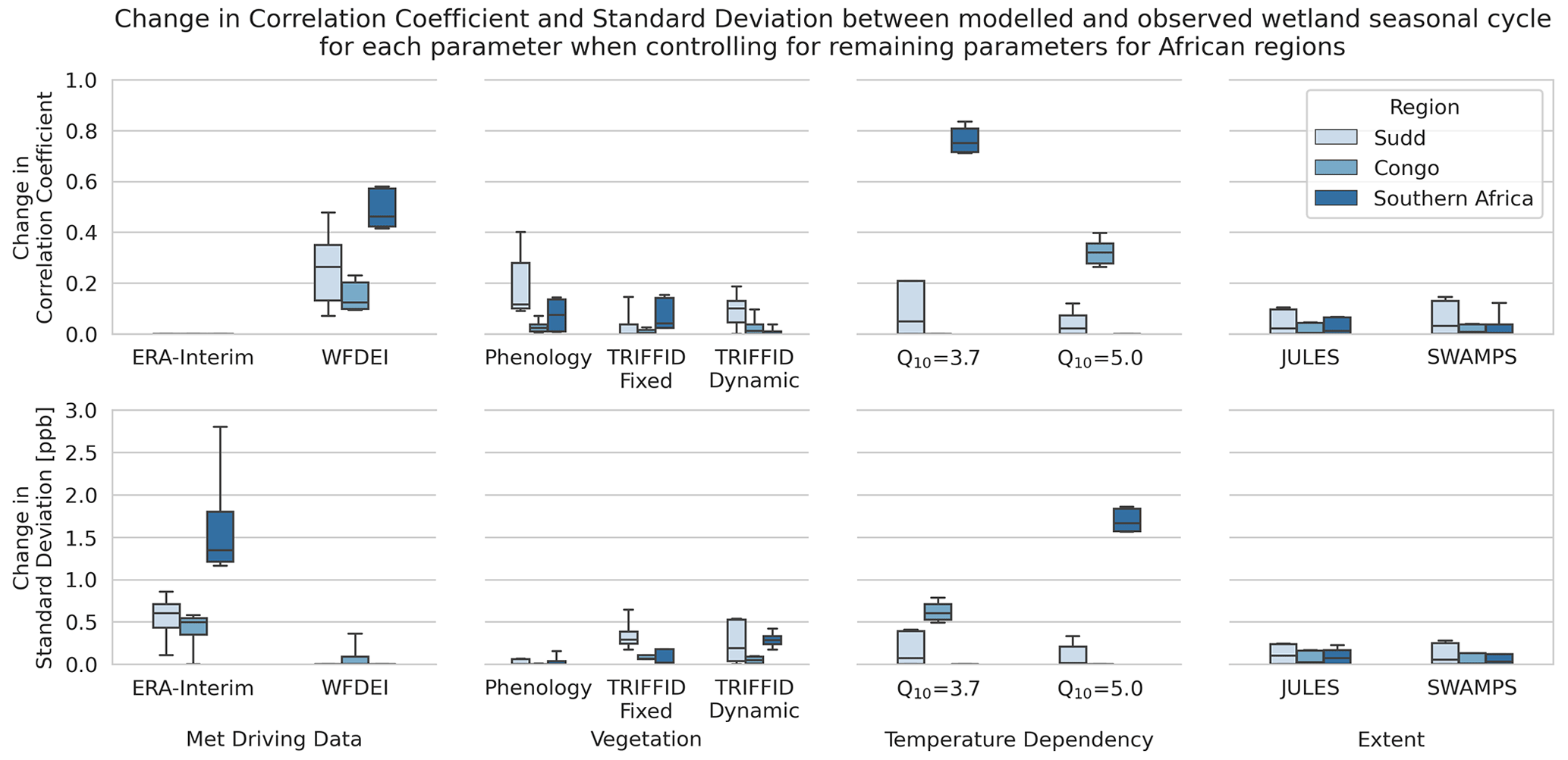
Figure 7The change in correlation coefficient (top) and standard deviation (bottom) between the JULES ensemble and GOSAT wetland CH4 seasonal cycle when controlling for the remaining ensemble parameters. The change is the difference above the minimum value for each set of ensemble members. An increased correlation coefficient should be considered an improvement, whereas an increased standard deviation should be considered a deterioration. The figure shows the changes for the three wetland regions that we examine over Africa (Sudd, Congo and Southern Africa) and are presented as box-and-whisker plots (box: quartiles; whiskers: min/max).
We now investigate three significant African wetland regions (the Sudd, the Congo and Southern Africa) in detail and evaluate the performance of the JULES wetland methane emission estimates in these regions. These regions were selected as they were found to exhibit particularly poor correlation coefficients between GOSAT and JULES, suggesting issues with the timing of the seasonal cycle, as well as large differences in seasonal cycle amplitude.
Figure 7 presents the same analysis as performed in Fig. 6 but broken down individually for the three African wetland regions. Overall, the same general pattern that we find for all regions persists individually for these regions but with some interesting exceptions.
For the meteorological data, the WFDEI ensemble members show improved ΔRcycle (0.26, 0.12 and 0.46 medians for Sudd, Congo and Southern Africa respectively) with ERA-Interim worsening the ΔσA value (by 0.60, 0.50 and 1.35 ppb respectively). As a reminder here, a value of zero (as is the case for the change in ERA-Interim) indicates that the selection consistently performs the same (be that the lowest correlation coefficient or the smallest standard deviation) in relation to the other possible selection(s).
For the vegetation configuration, as found across all regions combined, there is not a distinctly better configuration. The phenology-based ensemble members perform best for the Sudd, with the highest ΔRcycle (0.12) and lowest ΔσA (0.0 ppb, indicating that it consistently outperforms the other configurations). However, there seems to be very little improvement for the Congo region, or indeed variability, between the three different vegetation options. This is largely expected due to low variability/seasonality in the tropical broadleaf vegetation. For the Southern Africa region, the dynamic TRIFFID configuration performs slightly worse than the others (ΔσA increasing by 0.28 ppb), but the performance of phenology and fixed-TRIFFID is hard to differentiate.
The temperature dependency exhibits very strong regional behaviour. For example, for Southern Africa, the temperature dependency can improve ΔRcycle by 0.75 for the lower Q10 value vs. the higher value, and, at the same time, the higher Q10 value can worsen the ΔσA by over 1.6 ppb. In contrast, for the Congo, the higher Q10 value improves ΔRcycle by 0.32 with the lower Q10 value worsening ΔσA by over 0.6 ppb. While this does not leave us with a clear indication that one Q10 value is universally better than the other, it does highlight the potential for significantly improving the ΔRcycle via the selection of appropriate region-specific values. It should be noted that while some studies (e.g. Turetsky et al., 2014) have measured a wide variability in Q10 values across different wetland types (e.g. bog, fen and swamps), these have typically focused on subtropical, temperate and northern high-latitude regions. Further observations and constraints on the temperature dependency of tropical wetlands would be useful in this context.
Finally, neither configuration of wetland extent is found to significantly outperform the other for any of the three regions. For the Congo and Southern Africa regions, there is very little difference and very little improvement from selecting one extent configuration over the other. For the Sudd region, there is a slightly larger spread across the ensembles, but that is true for both the JULES and SWAMPS wetland extent configurations with neither significantly improving ΔRcycle nor worsening the ΔσA.
5.1 Additional datasets for African case study analysis
We find that several additional datasets offer utility in further diagnosing the wetland CH4 behaviour. This section briefly describes those datasets used in the case study analysis of African wetlands in Sects. 5.2–5.4.
5.1.1 Wetland emissions datasets
WetCHARTs (Bloom et al., 2017a) is a simple data-driven wetland model and one which has previously been extensively evaluated against satellite observations (Parker et al., 2020b). WetCHARTs is also commonly used as a priori information in atmospheric inversions of CH4 (Sheng et al., 2018; Lu et al., 2021; Palmer et al., 2021). As such, it can act as a useful benchmark against which to compare the JULES wetland emission estimates.
We also utilise emission estimates from a dedicated high-resolution () atmospheric inversion of GOSAT XCH4 (Lunt et al., 2021) using the GEOS-Chem model over sub-Saharan Africa. Emissions were estimated in a Bayesian inversion framework between 2010 and 2016. Emission priors for wetlands were taken from the WetCHARTs model, the EDGAR v4.3.2 database for anthropogenic emissions and the GFED v4.1s dataset for biomass burning emissions. Total CH4 emissions were resolved in the inversion from basis functions representing individual countries and major river basins. Posterior wetland emissions were estimated based on the fraction of prior emissions from wetlands in each grid cell, scaled by the posterior total CH4 emissions.
5.1.2 Wetland extent datasets
Wetland extent information can either be obtained from prognostic (model-based) or observation-based estimates.
We use the Wetland Area and Dynamics for Methane Modeling (WAD2M) wetland extent dataset (Zhang et al., 2021) which provides global estimates of wetland fraction for inundated and non-inundated vegetated wetlands, derived from microwave remote sensing. WAD2M is derived using a combination of surface inundation based on microwave remote sensing data along with static datasets that identify inland waters, agricultural areas, shorelines and non-inundated wetlands. Areas containing permanent waterbodies (e.g. lakes and rivers), rice paddies and coastal wetlands are excluded. Therefore, the resulting dataset represents the spatio-temporal patterns of inundated and non-inundated vegetated wetlands and is expected to improve estimates of wetland CH4 fluxes. In this study, we use the updated version which spans 2000–2018.
The global Catchment-based Macro-scale Floodplain (CaMa-Flood) v4.0 flood simulation model (Yamazaki et al., 2011; Zhou et al., 2021) was used to predict fluvial inundation extents, specifically simulations at a resolution driven by JULES runoff estimates from the eartH2Observe project (Marthews et al., 2022).
Finally, we also use surface reflectance imagery (RGB) from the MODIS satellite, processed and visualised using Google Earth Engine. These data allow a visual inspection of the region and provide a useful indicator of potential inundation, albeit not in the presence of dense vegetation canopy.
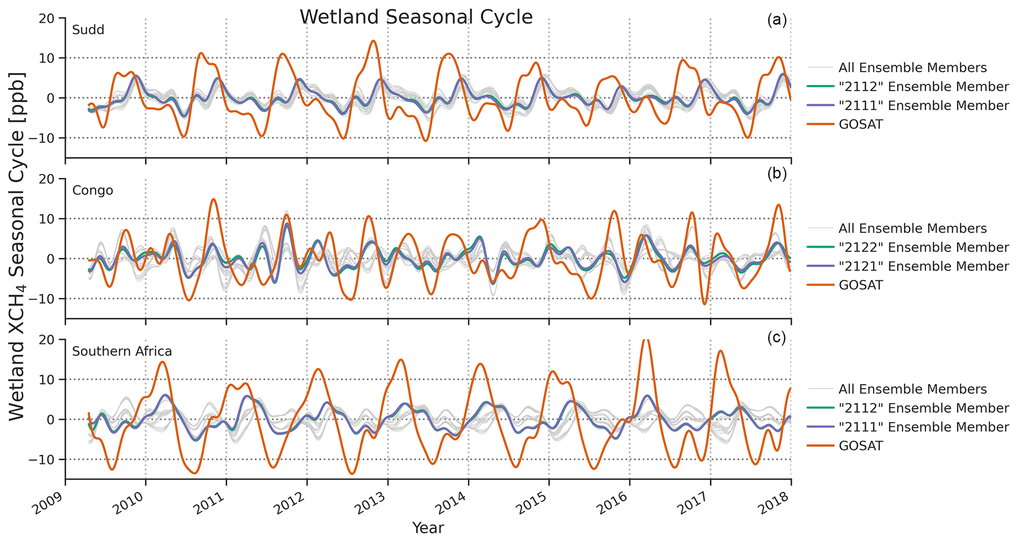
Figure 8Time series showing the GOSAT (red) and JULES ensemble (grey) wetland CH4 seasonal cycles for the three African wetland regions. The wetland seasonal cycle is calculated by subtracting the TOMCAT model simulations that do not contain any wetland emissions. For each region, the best performing (highest Rcycle) ensemble members are shown for the JULES and JULES-SWAMPS wetland extent configurations.
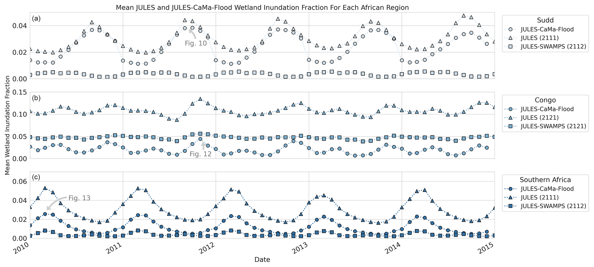
Figure 9Time series showing the mean fluvial inundation fraction generated by the CaMa-Flood model for the three African wetlands regions between 2010 and 2015 compared to the standard JULES groundwater inundation. The annotations highlight the example month chosen for each region that is subsequently presented in Figs. 10, 12 and 13.
5.1.3 Sentinel-5 Precursor (S5P) TROPOspheric Monitoring Instrument (TROPOMI) XCH4
We use XCH4 from v1.5 of the University of Bremen TROPOMI weighting function modified differential optical absorption spectroscopy (WFM-DOAS) retrieval (Schneising et al., 2019). Although the TROPOMI data are relatively new (Sentinel-5 Precursor launched in October 2017) and algorithm development is still maturing, TROPOMI does offer an unprecedented capability for the mapping of CH4 over large regions at an enhanced (7 km) spatial resolution and complements the long time series of GOSAT point-based measurements.
5.2 The Sudd
The first region that we focus on is the Sudd wetlands in South Sudan. The Sudd is one of the world's largest freshwater ecosystems and the largest in the Nile Basin, draining much of Eastern Africa, including water from Lake Victoria (Sutcliffe and Brown, 2018). This outflow from Lake Victoria leads to strong seasonal inundation, characterised by annual flood pulses (Rebelo et al., 2012), that is further modified by local precipitation and evaporation (Mohamed and Savenije, 2014), leading to highly complex and seasonal behaviour (Sosnowski et al., 2016). Previous work (Parker et al., 2020a; Lunt et al., 2021; Pandey et al., 2021) has detailed the importance of understanding and characterising the CH4 emissions from the Sudd wetlands given their sensitivity to large-scale climate drivers.
As discussed in Sect. 5, we find that neither parameterisation of wetland extent (JULES nor JULES masked with SWAMPS) outperforms the other for all three African regions, and, as shown in Fig. 5, the correlation coefficient between the ensemble members and observations is poor. Although the WFDEI driving data greatly improve the correlation coefficient compared with ERA-Interim, the ensemble members with the best performance are only capable of achieving an Rcycle value of 0.61 (Fig. A2). It is interesting to note here that, for the Sudd, the ensemble members that perform best against observations (2121/2122: WFDEI, phenology and high temperature dependency) are the exceptions from the ensemble. The majority of the ensemble members correlate well with each other and poorly with the observations. Figure 8a shows the wetland seasonal cycle for the individual ensemble members and includes the observed seasonal cycle. The wetland seasonal cycle amplitude (AJULES) even for the ensemble member with the best performance is significantly lower than the observed seasonal cycle (AGOSAT), as summarised in Fig. 5, and the reason for the poor Rcycle value is that JULES appears to be out of phase with observations. These findings all suggest that a fundamental lack of variability is being generated by JULES, with wetland extent an obvious parameter to evaluate in greater detail.
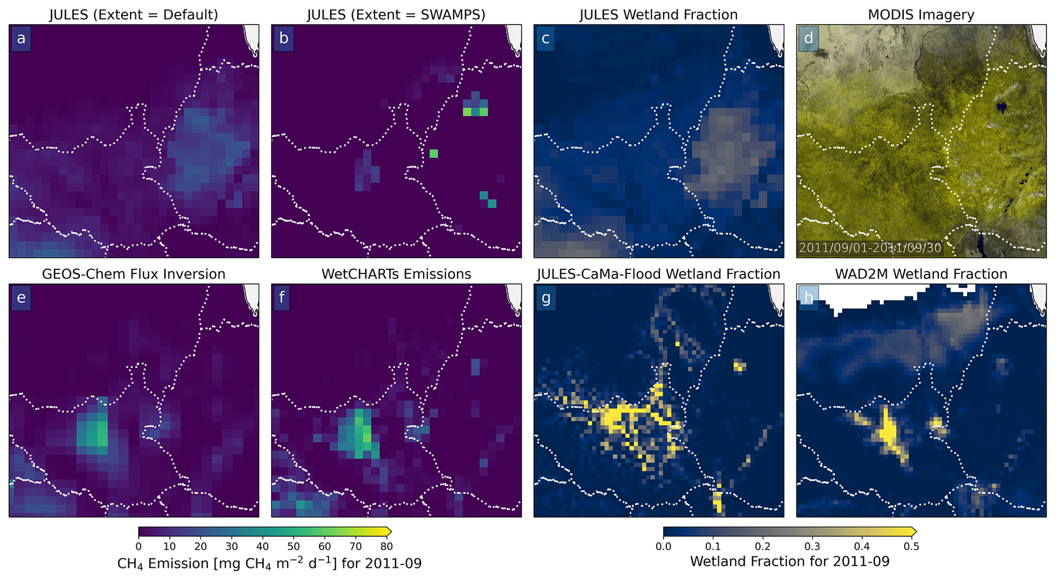
Figure 10Comparison over the Sudd wetland region showing the wetland CH4 emissions for September 2011 for (a) JULES with the default wetland extent, (b) JULES with the SWAMPS masking for wetland extent, (e) GEOS-Chem flux inversion of GOSAT XCH4 over Africa and (f) the WetCHARTs ensemble mean. Also shown are the wetland fractions from (c) JULES, (g) JULES-CaMa-Flood and (h) WAD2M along with (d) MODIS (RGB) surface reflectance. Both JULES simulations are the configurations that use the WFDEI meteorological driving, the lower Q10 value and phenological vegetation, as these were shown to provide the best result over this region (see Fig. 7).
In Fig. 9, we compare the JULES wetland fraction for these three regions against that generated using JULES-CaMa-Flood simulations that are capable of explicitly representing river and floodplain water dynamics and, hence, incorporate fluvial inundation. CaMa-Flood is the only open-source global river routing model that is based on the local inertial approximation of the Saint-Venant equations, which consider the backwater and tide effects of downstream elements (viz. the possible reversal of flow in particular reaches upstream from e.g. lakes, tributaries and estuaries) (Marthews et al., 2022).
For the Sudd, we find that the wetland extent seasonal cycle and magnitude are very similar between JULES and JULES-CaMa-Flood. However, applying the SWAMPS mask to JULES results in the JULES-SWAMPS configuration having a drastically smaller seasonal cycle amplitude and a significantly different phase (almost completely out of phase). This suggests that simply applying the JULES-SWAMPS mask for the Sudd results in a decoupling of the seasonal cycle for the masked areas from the wider region. For this reason, we evaluate the spatial distribution of both the CH4 emissions and the wetland extent. Figure 10 focuses on September 2011, which is towards the peak of the inundation, as indicated by the JULES-CaMa-Flood simulations (Fig. 9). In Fig. 10, we present CH4 emission maps over the Sudd from two of the JULES ensemble members: one with the default wetland extent (Fig. 10a) and one with the additional SWAMPS mask (Fig. 10b). Furthermore, we also show the CH4 emissions derived from a GEOS-Chem flux inversion (Fig. 10e) and from the WetCHARTs ensemble (Fig. 10f). In addition to the CH4, we show the JULES wetland fraction (Fig. 10c), MODIS imagery (Fig. 10d), the JULES-CaMa-Flood wetland fraction (Fig. 10g) and the WAD2M wetland fraction (Fig. 10h). By using this wide range of information, we are able to more confidently assess and evaluate the performance of JULES in this region and determine whether wetland area (and subsequently CH4 emissions) are being generated in the correct locations.
There is an obvious discrepancy between the area where JULES generates wetland area (and subsequently CH4 emission) compared with the location indicated by all of the other datasets. JULES places the majority of wetlands in the region in western Ethiopia (Fig. 10c) and fails to generate significant wetlands in South Sudan. All of the other data sources agree strongly with respect to where the wetlands and emissions should be located (Fig. 10d–h), with the majority over the Sudd wetlands in central South Sudan and additional wetlands in the Machar marshes on the border with Ethiopia (e.g. Fig. 10h). When using the SWAMPS masking of the JULES wetland extent, slightly more emissions are generated in the correct location due to the removal of the majority of the spurious Ethiopian emissions, but emissions remain significantly too low with respect to both area and magnitude.
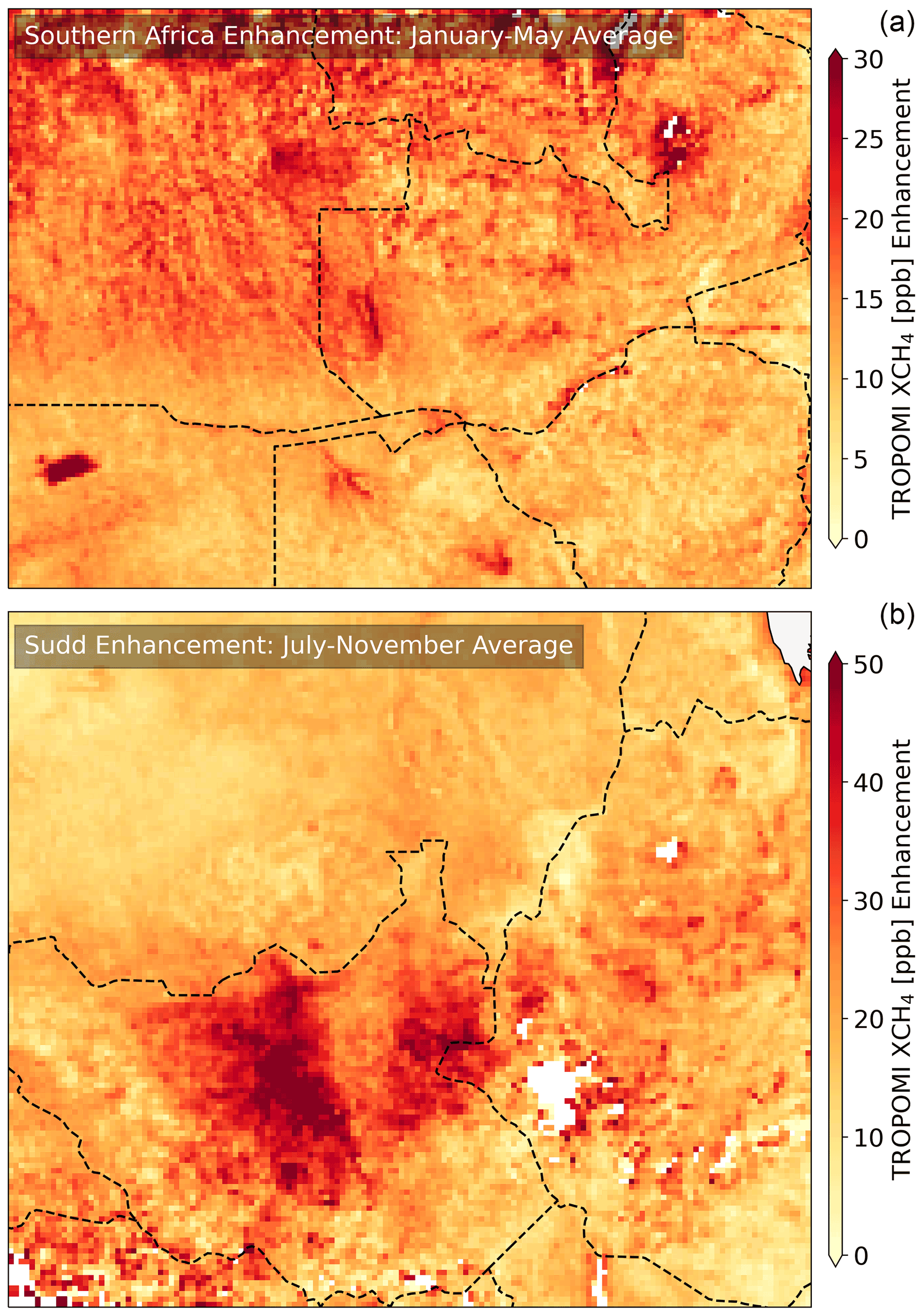
Figure 11Enhancement in TROPOMI XCH4 calculated by gridding the data into daily bins and subtracting a baseline for each latitude bin. The baseline is calculated as the 5th percentile of each latitude bin with a rolling five-bin (i.e. 0.5∘ latitude) average used to smooth out fluctuations. The enhancements are shown for the Southern Africa and Sudd regions, averaged over the months where the wetland signal peaks, as indicated in Fig. 8. For Southern Africa, it should be noted that the enhancement over the Etosha Pan in Namibia (south-west corner of the domain) is likely overestimated due to particular spectral albedo variations within the fitting window used in the satellite retrievals. Finally, there were not sufficient cloud-free observations for the Congo region.
As further confirmation of where CH4 emissions should be present in this region, CH4 observations from TROPOMI are used, allowing us to map CH4 in the region. Figure 11b shows the enhancement in the TROPOMI data over the Sudd region, calculated by subtraction of latitudinal means, between January and May for 2018–2020. This clearly shows a strong enhancement in the measured CH4 total column (in excess of 45 ppb) at the location, consistent with our above interpretation, directly over the Sudd wetlands as well as an enhancement over the Machar marshes. Pandey et al. (2021) have previously shown a similar enhancement from TROPOMI over this region, adding further weight to our conclusions.
The reason that JULES fails to produce these wetlands is largely due to the topography in this region. Rainfall here occurs in the Ethiopian Highlands, flowing downhill to maintain the Sudd wetlands. Without the addition of a river routing and inundation mechanism within the JULES simulations, wetlands are instead created erroneously in the Ethiopian Highlands (as indicated in Fig. 10a).
It is important to highlight here that the JULES-CaMa-Flood simulations (Fig. 10g) are capable of producing wetlands in the correct location; as such, future developments within JULES that incorporate some of the CaMa-Flood capabilities for river routing and fluvial inundation would be expected to significantly improve the ability of JULES to successfully reproduce the correct temporal and spatial distribution of wetlands (and ultimately CH4 emissions) over the Sudd region.
5.3 The Congo
The second region that we focus on is the Congo. The Congo Basin contains flooded forests and peatlands, known as the “Cuvette Centrale”, which act as a major global store of carbon (Dargie et al., 2017) and source of CH4 emissions (Borges et al., 2015). CH4 emissions from the Congo are still poorly constrained (Melton et al., 2013), with dense cloud cover and forest canopies making observations of both wetland extent (Salovaara et al., 2005; Bwangoy et al., 2010; Becker et al., 2018) and CH4 emissions challenging (Tathy et al., 1992; Lunt et al., 2019; Parker et al., 2020b). The complex hydrology (Lee et al., 2011) in this region includes two wet seasons, in March and November (Haensler et al., 2013), making coupled climate simulations of this region challenging (Crowhurst et al., 2021).
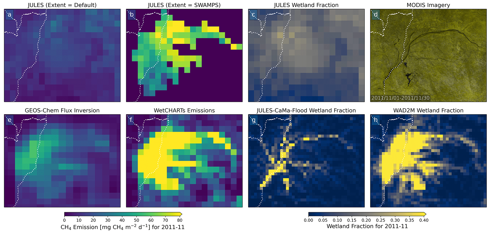
Figure 12Comparison over the Congo wetland region showing the wetland CH4 emissions for November 2011 for (a) JULES with the default wetland extent, (b) JULES with the SWAMPS masking for wetland extent, (e) GEOS-Chem flux inversion of GOSAT XCH4 over Africa and (f) the WetCHARTs ensemble mean. Also shown are the wetland fractions from (c) JULES, (g) JULES-CaMa-Flood and (h) WAD2M along with (d) MODIS (RGB) surface reflectance. Both JULES simulations are the configurations that use the WFDEI meteorological driving, the higher Q10 value and phenological vegetation, as these were shown to provide the best result over this region (see Fig. 7).
Figure 8b shows the modelled ensemble seasonal cycle along with the observed seasonal cycle. Again, the highest correlation coefficient for an ensemble member is found to be poor (Rcycle=0.52), with some ensemble members exhibiting zero correlation to the observations. This again suggests a significant lack of seasonal variability in the JULES simulations. Furthermore, the observed seasonality exhibits more complex behaviour with double-peaks in some (but not all) years, highlighting the complex hydrology in this region.
Figure 9b shows that the seasonality produced by JULES-CaMa-Flood is in good agreement with that from JULES but with significantly lower average inundation (∼0.02 vs. ∼0.10). When applying the SWAMPS mask to JULES, the average inundation is reduced (to ∼0.05) and the seasonality is largely lost.
By undertaking a comparison against the additional datasets, we see why the Congo remains a difficult area to model. The default JULES simulations result in groundwater inundation of the entire Congo Basin (Fig. 12c), leading to fairly low widespread emissions, whereas the JULES simulations with the extent masked by SWAMPS produce significantly more emissions (Fig. 12b), which are more tightly constrained to the area in the vicinity of the river system, although still very widespread. These latter emissions with the SWAMPS mask do appear to be in more reasonable agreement spatially with the CH4 emissions from both the GEOS-Chem inversion (Fig. 12e) and from WetCHARTs (Fig. 12f). Some care needs to be taken here because WetCHARTs itself is used as the prior for the GEOS-Chem flux inversion; thus, the two should not be considered fully independent, and the major difference between them is reflected in the emissions magnitude. The fluvial inundation from the JULES-CaMa-Flood simulations over the Congo (Fig. 12g) produces a wetland extent close to the river, which is largely missing from the standard JULES simulations. MODIS imagery (Fig. 12d) agrees with the JULES-CaMa-Flood simulations and does not show clear signs of inundation over this area except directly at the rivers. However, this may be misleading due to the dense tree canopy in this area. Indeed, wetlands (i.e. swamps and flooded forest) in the Congo can exist in relatively hilly areas that are not directly fed by river flooding but more by local precipitation or groundwater. The pattern of wetland fraction from WAD2M (Fig. 12h), employing microwave observations that can partially penetrate the canopy layer, does suggest that there is a combination of both groundwater inundation and fluvial inundation. This does highlight the challenge in simulating such flooded forests, where evaluation can be challenging and observations lacking. Additionally, dense cloud cover in this region results in very few successful CH4 retrievals from satellites (both GOSAT and TROPOMI), again reducing our capability to accurately evaluate model performance in this region.
The Congo remains one of the most significant global wetland regions but equally remains one of the most challenging to simulate and evaluate, with a significant uncertainty in the CH4 emissions. Ongoing model development (Gedney et al., 2019) related to the inclusion of methane emissions from trees in flooded areas (Pangala et al., 2017; Gauci et al., 2022) as well as improvements in the soil ancillary data to represent Oxisol and Ultisol soils in this area are expected to improve our ability to more accurately model the CH4 emissions from the Congo in future work.
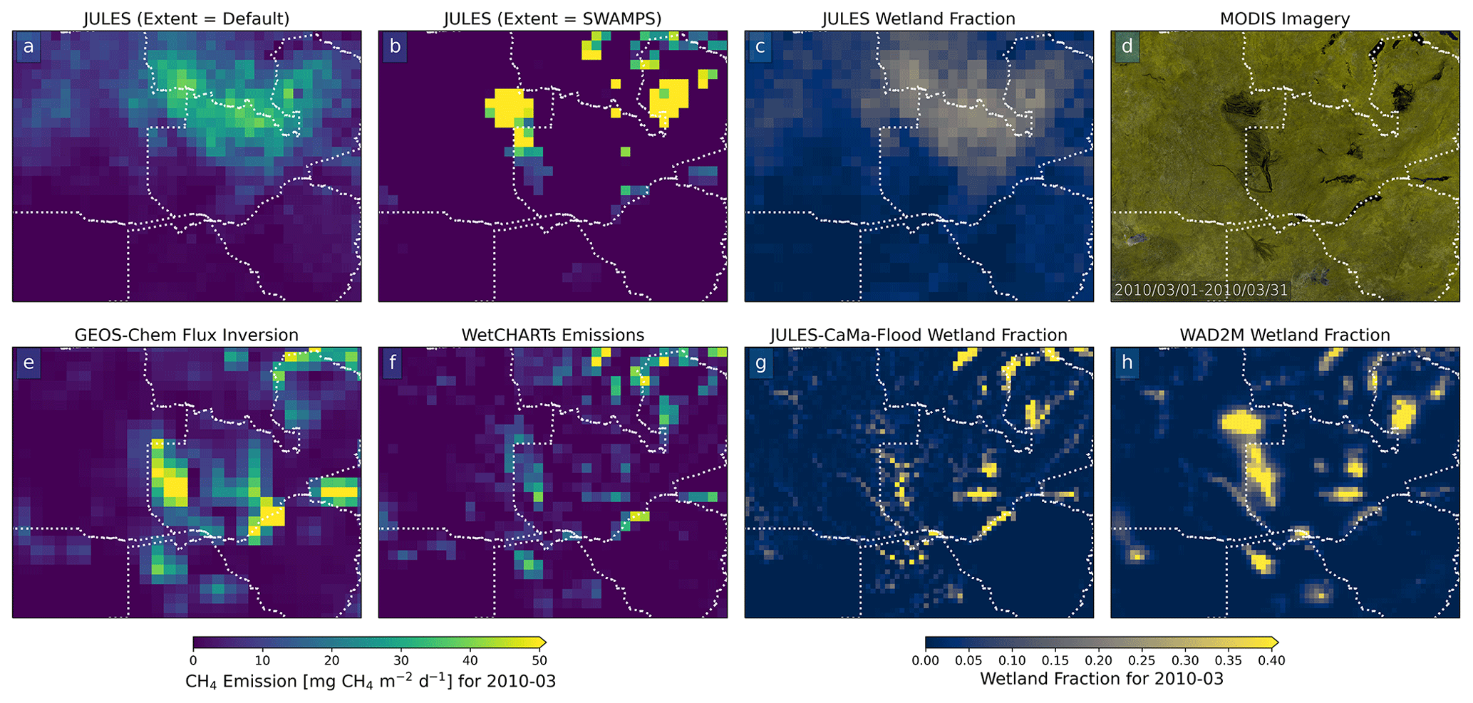
Figure 13Comparison over the Southern Africa wetland region showing the wetland CH4 emissions for March 2010 for (a) JULES with the default wetland extent, (b) JULES with the SWAMPS masking for wetland extent, (e) GEOS-Chem flux inversion of GOSAT XCH4 over Africa and (f) the WetCHARTs ensemble mean. Also shown are the wetland fractions from (c) JULES, (g) JULES-CaMa-Flood and (h) WAD2M along with (d) MODIS (RGB) surface reflectance. Both JULES simulations are the configurations that use the WFDEI meteorological driving, the lower Q10 value and phenological vegetation, as these were shown to provide the best result over this region (see Fig. 7).
5.4 Southern Africa
The final region that we evaluate is Southern Africa, primarily focusing on the Zambezi River basin in Zambia and Angola but also including parts of Namibia, Botswana, Zimbabwe, Mozambique and the Democratic Republic of Congo. Wetlands in this region are primarily swampland and seasonally inundated savannah/grasslands (Zimba et al., 2018; Lowman et al., 2018). The region also encompasses the Okavango Delta in northern Botswana (McCarthy, 2006; Wolski et al., 2012).
The values of Rcycle for this region are found to vary significantly, ranging from reasonable positive correlations (Rcycle=0.67) to similar large negative correlations (). This region is one in particular where the WFDEI-based ensemble members perform much better than the ERA-Interim members, as shown in Fig. 7.
Figure 8c shows that there is a reasonable correlation (maximum of 0.67) to the observed cycle for the ensemble members with the largest Rcycle value. However, this is countered by some ensemble members having a similarly negative Rcycle value (of −0.68 in the worst case). All of the ERA-Interim-based ensemble members have a low or negative Rcycle value (), whereas the WFDEI ensemble members range from −0.23 to 0.67. This very wide spread in Rcycle () across the ensemble explains why the average correlation is found to be very poor (Fig. 5).
When comparing the wetland extent from the ensemble members that show the best performance to that produced by JULES-CaMa-Flood (Fig. 9c) we find a good agreement in the seasonality between all three. However, in terms of the magnitude, the average groundwater inundation for the default JULES configuration is augmented by approximately 50 % in the simulation with JULES-CaMa-Flood, with the SWAMPS-masked inundation, in contrast, being far too low. Figure 13 clarifies the fact that, although the seasonality is reasonable, the spatial distribution is again incorrect. The default JULES wetland extent for this region places wetlands in northern Zambia and in the southern Democratic Republic of Congo. In contrast, the SWAMPS mask places the wetlands primarily along the Zambezi and Bangweulu wetlands in the west and north-east of Zambia respectively. The flux inversion results from GEOS-Chem suggest that emissions are observed over the Zambezi floodplain but also over various other locations in the region, including the Okavango Delta to the south, around Lake Kariba along the Zambia–Zimbabwe border, the Cahora Bassa lake in Mozambique and the Bangweulu wetland system in north-east Zambia. The WAD2M wetland fractions and the MODIS imagery both also indicate these as being significantly inundated areas. Although the methane enhancement signals (20–30 ppb) are not as large as identified for the Sudd region, the TROPOMI S5P CH4 enhancement (Fig. 11) does indicate enhanced CH4 values over these areas, thereby giving further confidence that the inundated areas are being correctly identified along with their subsequent CH4 emission by the GEOS-Chem flux inversion. The wetland fraction calculated by the JULES-CaMa-Flood simulation (Fig. 13g) is found to be in very good agreement with the WAD2M data (Fig. 13g) and, hence, suggests that JULES CH4 emissions based on the JULES-CaMa-Flood-derived wetlands would be in much closer agreement with the observations.
Overall, we find that existing configurations of JULES can simulate wetland CH4 emissions comparable in performance to those generated via state-of-the-art data-driven emission inventories such as WetCHARTs.
The wetland methane seasonal cycle amplitude from JULES is typically underestimated by between 1.8 and 19.5 ppb compared with observations across the different wetland regions examined. However, the correlation coefficient to the observed seasonal cycle is typically reasonable to good for most wetland regions (r=0.58 to 0.88), although several regions do exhibit a poor correlation (r<0.31) and these are explored in more detail.
Across the JULES ensemble, there are significant differences between ensemble members with the WFDEI driving data giving universally better performance than ERA-Interim. This highlights the vital role that the meteorological driving input data play in determining the wetland response within the model and emphasises the benefits of bias-correcting to observations as done in the generation of the WFDEI data. We would expect our conclusions regarding the strong performance of WFDEI meteorology to also apply to the updated WFDE5 data (based on ERA5), detailed in Cucchi et al. (2020). Future work will assess simulations driven by these inputs.
We find that the specific vegetation configuration of the ensemble member has a small effect on the performance (with phenology typically performing better than either TRIFFID configuration), suggesting that there are potential improvements to consider when using a dynamic vegetation model such as TRIFFID. The effect of the temperature dependency is moderate, with the lower value (Q10=3.7) generally performing best, but there are some important regional differences where the effect is much larger. We recommend further investigation into the variability in Q10 across different ecosystems and the consequences that has for CH4 emissions.
Neither choice of wetland extent, either the original JULES as is or masked with SWAMPS data, tends to perform better, and both clearly have significant deficiencies. We find that a simple masking of the JULES wetland extent with the observed SWAMPS wetland mask is not sufficient to reproduce the wetland seasonal cycle in key areas; instead, fundamental changes to the way the inundation is modelled are necessary in some regions, particularly those regions where fluvial inundation plays a significant role in the hydrology. This is demonstrated by the significant improvement in the agreement to multiple observation-based wetland and CH4 datasets when using the JULES-CaMa-Flood wetland extent, which incorporates fluvial inundation, compared with the original (interfluvial) JULES data over key African wetland regions. Incorporating such fluvial inundation changes into JULES is expected to significantly improve the ability of JULES to better represent the wetland extent and, subsequently, produce more accurate CH4 emissions.
Despite our analysis pointing towards the potential for significant improvements in key regions, the Congo wetland region in particular remains both challenging to model and to evaluate, highlighting the need for further study and additional ground-based observations that are less affected by the extensive cloud coverage of the region. Improved mapping of the wetland extent (by both groundwater and fluvial inundation) as well as measurements of the temperature dependency of the CH4 emissions would help in further constraining the CH4 emissions from this region.
Finally, ongoing developments within JULES, such as the chimney venting (i.e. transport by aerenchyma) of CH4 by vegetation and the improved representation of soil properties, are expected to lead to additional improvements in the model. With these additions coupled to an improved representation of wetland extent and variability through more advanced hydrological modelling, we greatly improve our capability to model the emission of CH4 from tropical wetlands both historically and under a changing future climate.
In the main text (Sect. 4), we refer to previous work (Parker et al., 2020b) that evaluates the WetCHARTs data-driven emission inventory (Bloom et al., 2017a) using a similar methodology as used in this study. This common analysis methodology allows a direct comparison between the performance of the JULES wetland CH4 emissions (this study) and the WetCHARTs performance (Parker et al., 2020b). Figure A1 reproduces Fig. 5 from this study and compares it to Fig. 4 from Parker et al. (2020b).

Figure A1Comparison of Fig. 5 from this study for JULES against Fig. 4 from Parker et al. (2020b) for WetCHARTs.
Figure A2 shows the correlation coefficient between the different ensemble members and the observed wetland CH4 seasonal cycle for the Sudd region. The majority of the ensemble members correlate strongly to each other (r>0.9) but poorly to the observed seasonal cycle (r<0.2). The set of ensemble members that correlates best to observations (members 2121 and 2122 – WFDEI meteorology, phenology vegetation and high Q10 value) correlates the least to the remaining ensemble members, suggesting a significant difference in the characteristics of these few ensemble members. This is discussed in the main text in Sect. 5.2.

Figure A2Correlation coefficient between the different ensemble members and the observed wetland CH4 seasonal cycle for the Sudd wetland region.
We perform additional assessment on the assumptions made in our methodology when calculating the wetland seasonal cycle signal, specifically assumptions relating to the accuracy of non-wetland sources.
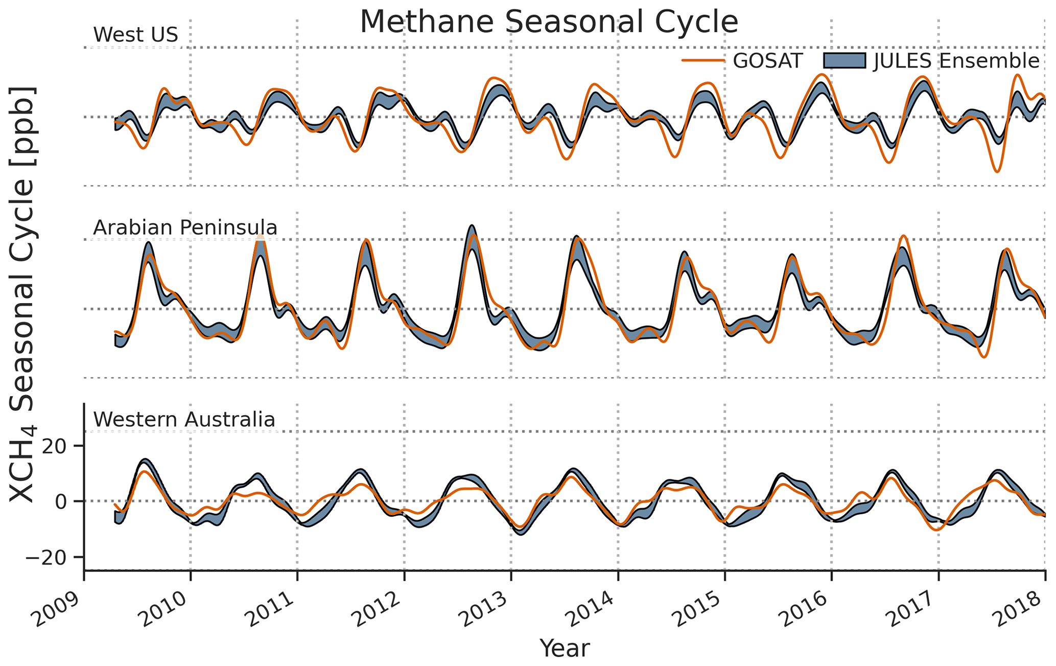
We have performed analysis over three non-wetland areas (as highlighted in red in Fig. B1), namely the West US, Arabian Peninsula and Western Australia. These regions would not be expected to be dominated by wetland emissions; hence, evaluation of the simulated CH4 column against observations provides an assessment of how the non-wetland emissions in the model are performing. The detrended methane seasonal cycle (note that this is the total, not wetland-only) for the model is compared against GOSAT observations in Fig. B2, and we find a very good agreement (with correlation coefficients of 0.89, 0.96 and 0.90 for the West US, Arabian Peninsula and Western Australia respectively). This, along with previous work as outlined in Sect. 4, provides confidence that the current model set-up and associated priors provide a strong baseline against which to assess the wetland-specific component of the observed/modelled signal.
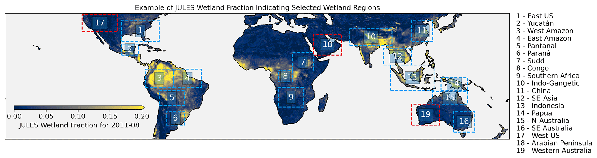
Figure B1An adjusted version of Fig. 3 showing the locations of the 16 wetland regions considered in this study plus 3 additional non-wetland regions (in red). A representative month (August 2011) of the JULES wetland fraction is shown as the basemap.
For this study, we use version 5.1 of JULES (at revision 10836, released in February 2018). The source code is available from the JULES code repository (see https://code.metoffice.gov.uk/trac/jules/log/main/trunk?rev=10836, UK Met Office, 2022a, user account required). The rose suites used for the specific JULES runs are u-ba800 (WFDEI+phenology), u-bh665 (WFDEI+TRIFFID no competition), u-ax384 (WFDEI+TRIFFID), u-be476 (ERA-Interim+phenology), u-be478 (ERA-Interim+TRIFFID no competition) and u-be517 (ERA-Interim+TRIFFID). The rose suites can be found at https://code.metoffice.gov.uk/trac/roses-u/ (UK Met Office, 2022b) (user account required). We run each rose suite twice, using Q10 values of 3.7 and 5.0.
The latest version of the University of Leicester GOSAT Proxy v9.0 XCH4 data (Parker and Boesch, 2020) is available from the Centre for Environmental Data Analysis data repository at https://doi.org/10.5285/18ef8247f52a4cb6a14013f8235cc1eb. The version used in this study (v7.2) is available from the Copernicus C3S Climate Data Store at https://doi.org/10.24381/cds.b25419f8 (ECMWF, 2022). WetCHARTs v1.0 is available from https://doi.org/10.3334/ORNLDAAC/1502 (Bloom et al., 2017b). This study uses v1.2.1, which is available on request from A. Bloom. WAD2M is available from https://doi.org/10.5281/zenodo.3998454 (Zhang et al., 2020). The MODIS Surface Reflectance 8-Day L3 data and MODIS Combined 16-Day NDWI data were visualised via the Google Earth Engine software with the data provided courtesy of the NASA Earth Observing System Data and Information System (EOSDIS) Land Processes Distributed Active Archive Center (LP DAAC), USGS/Earth Resources Observation and Science (EROS) Center, Sioux Falls, South Dakota (https://lpdaac.usgs.gov, last access: 13 December 2020).
The University of Bremen TROPOMI/WFM-DOAS XCH4 data are available from https://www.iup.uni-bremen.de/carbon_ghg/products/tropomi_wfmd/ (Schneising, 2022).
Requests for information about the code, data and parameterisations can be made to the corresponding author.
RJP generated the GOSAT XCH4 retrievals, performed the analysis and drafted the manuscript. AAB produced an updated version of the WetCHARTs dataset for use in this study. CW and MPC produced the TOMCAT model simulations. GH and ECP generated the JULES simulations usage. TRM generated the JULES-CaMa-Flood simulations. MFL and PIP performed the GEOS-Chem flux inversion. All co-authors contributed to the planning and discussion of this study and to refining the manuscript.
The contact author has declared that none of the authors has any competing interests.
Publisher’s note: Copernicus Publications remains neutral with regard to jurisdictional claims in published maps and institutional affiliations.
Robert J. Parker, Hartmut Boesch, Chris Wilson, Martyn P. Chipperfield and Paul I. Palmer are funded via the UK National Centre for Earth Observation (grant nos. NE/R016518/1 and NE/N018079/1). The authors acknowledge support from the UK Natural Environment Research Council via the following grants and awards: The Global Methane Budget (MOYA; grant nos. NE/N015681/1, NE/N015657/1 and NE/N015746/1), The UK Earth System Modelling project (grant no. NE/N017951/1), TerraFIRMA (grant no. NE/W004895/1) and Hydro-JULES (grant no. NE/S017380/1). Nicola Gedney acknowledges support from the UK NERC (subcontract no. NEC05779) as part of The Global Methane Budget MOYA consortium. NG was also supported by the Newton Fund through the Met Office Climate Science for Service Partnership Brazil (CSSP Brazil). Part of this research was carried out at the Jet Propulsion Laboratory, California Institute of Technology, under a contract with the National Aeronautics and Space Administration. Funding for the WetCHARTs emissions was provided through a NASA Carbon Monitoring System grant (grant no. NNH14ZDA001N-CMS). We also acknowledge funding from the ESA GHG-CCI and Copernicus C3S projects (grant no. C3S2_312a_Lot2).
This research used the ALICE high-performance computing facility at the University of Leicester for the GOSAT retrievals and analysis. We undertook the JULES runs on the NERC's JASMIN high-performance computing facility. The TOMCAT simulations were performed on the national Archer and Leeds Arc high-performance computing systems.
This publication contains modified Copernicus Sentinel data (2018, 2019, 2020). Sentinel-5 Precursor is an ESA mission implemented on behalf of the European Commission. The TROPOMI payload is a joint development by the ESA and the Netherlands Space Office (NSO). Sentinel-5 Precursor ground-segment development has been funded by the ESA and with national contributions from the Netherlands, Germany and Belgium. The generation of the TROPOMI methane product by University of Bremen has been funded by ESA (GHG−CCI+ project) and by the State and the University of Bremen.
We thank the Japanese Aerospace Exploration Agency, National Institute for Environmental Studies and the Ministry of Environment for the GOSAT data and their continuous support as part of the Joint Research Agreement.
This research has been supported by the National Centre for Earth Observation (grant nos. NE/R016518/1 and NE/N018079/1), the Natural Environment Research Council (The Global Methane Budget, grant nos. NE/N015681/1, NE/N015657/1, and NE/N015746/1, the UK Earth System Modelling project, grant no. NE/N017951/1, Hydro-JULES, grant no. NE/S017380/1, TerraFIRMA, grant no. NE/W004895/1, and UK NERC, subcontract no. NEC05779), the Earth Sciences Division (grant no. NNH14ZDA001N-CMS), and the ESA GHG-CCI and Copernicus C3S projects (grant no. C3S2_312a_Lot2).
This paper was edited by Martin De Kauwe and reviewed by Joe Melton and two anonymous referees.
Becker, M., Papa, F., Frappart, F., Alsdorf, D., Calmant, S., da Silva, J. S., Prigent, C., and Seyler, F.: Satellite-Based Estimates of Surface Water Dynamics in the Congo River Basin, Int. J. Appl. Earth Obs., 66, 196–209, https://doi.org/10.1016/j.jag.2017.11.015, 2018. a
Berchet, A., Pison, I., Chevallier, F., Paris, J.-D., Bousquet, P., Bonne, J.-L., Arshinov, M. Y., Belan, B. D., Cressot, C., Davydov, D. K., Dlugokencky, E. J., Fofonov, A. V., Galanin, A., Lavrič, J., Machida, T., Parker, R., Sasakawa, M., Spahni, R., Stocker, B. D., and Winderlich, J.: Natural and anthropogenic methane fluxes in Eurasia: a mesoscale quantification by generalized atmospheric inversion, Biogeosciences, 12, 5393–5414, https://doi.org/10.5194/bg-12-5393-2015, 2015. a
Best, M. J., Pryor, M., Clark, D. B., Rooney, G. G., Essery, R. L. H., Ménard, C. B., Edwards, J. M., Hendry, M. A., Porson, A., Gedney, N., Mercado, L. M., Sitch, S., Blyth, E., Boucher, O., Cox, P. M., Grimmond, C. S. B., and Harding, R. J.: The Joint UK Land Environment Simulator (JULES), model description – Part 1: Energy and water fluxes, Geosci. Model Dev., 4, 677–699, https://doi.org/10.5194/gmd-4-677-2011, 2011. a, b, c
Beven, K. J.: Rainfall-Runoff Modelling: The Primer, 2nd Edition, Wiley, ISBN 9780470714591, 2012. a
Beven, K. J., Kirkby, M. J., Freer, J. E., and Lamb, R.: A history of TOPMODEL, Hydrol. Earth Syst. Sci., 25, 527–549, https://doi.org/10.5194/hess-25-527-2021, 2021. a
Bloom, A. A., Palmer, P. I., Fraser, A., Reay, D. S., and Frankenberg, C.: Large-Scale Controls of Methanogenesis Inferred from Methane and Gravity Spaceborne Data, Science, 327, 322–325, https://doi.org/10.1126/science.1175176, 2010. a
Bloom, A. A., Bowman, K. W., Lee, M., Turner, A. J., Schroeder, R., Worden, J. R., Weidner, R., McDonald, K. C., and Jacob, D. J.: A global wetland methane emissions and uncertainty dataset for atmospheric chemical transport models (WetCHARTs version 1.0), Geosci. Model Dev., 10, 2141–2156, https://doi.org/10.5194/gmd-10-2141-2017, 2017a. a, b, c
Bloom, A. A., Bowman, K. W., Lee, M., Turner, A. J., Schroeder, R., Worden, J. R., Weidner, R. J., Mcdonald, K. C., and Jacob, D. J.: CMS: Global 0.5-Deg Wetland Methane Emissions and Uncertainty (WetCHARTs v1.0), ORNL DAAC, Oak Ridge, Tennessee, USA, WetCHARTs [data set], https://doi.org/10.3334/ORNLDAAC/1502, 2017b. a
Borges, A. V., Darchambeau, F., Teodoru, C. R., Marwick, T. R., Tamooh, F., Geeraert, N., Omengo, F. O., Guérin, F., Lambert, T., Morana, C., Okuku, E., and Bouillon, S.: Globally Significant Greenhouse-Gas Emissions from African Inland Waters, Nat. Geosci., 8, 637–642, https://doi.org/10.1038/ngeo2486, 2015. a
Bwangoy, J.-R. B., Hansen, M. C., Roy, D. P., Grandi, G. D., and Justice, C. O.: Wetland Mapping in the Congo Basin Using Optical and Radar Remotely Sensed Data and Derived Topographical Indices, Remote Sens. Environ., 114, 73–86, https://doi.org/10.1016/j.rse.2009.08.004, 2010. a
Chipperfield, M. P.: New Version of the TOMCAT/SLIMCAT off-Line Chemical Transport Model: Intercomparison of Stratospheric Tracer Experiments, Q. J. Roy. Meteor. Soc., 132, 1179–1203, https://doi.org/10.1256/qj.05.51, 2006. a
Clark, D. B., Mercado, L. M., Sitch, S., Jones, C. D., Gedney, N., Best, M. J., Pryor, M., Rooney, G. G., Essery, R. L. H., Blyth, E., Boucher, O., Harding, R. J., Huntingford, C., and Cox, P. M.: The Joint UK Land Environment Simulator (JULES), model description – Part 2: Carbon fluxes and vegetation dynamics, Geosci. Model Dev., 4, 701–722, https://doi.org/10.5194/gmd-4-701-2011, 2011. a, b, c, d, e, f
Comyn-Platt, E., Hayman, G., Huntingford, C., Chadburn, S. E., Burke, E. J., Harper, A. B., Collins, W. J., Webber, C. P., Powell, T., Cox, P. M., Gedney, N., and Sitch, S.: Carbon Budgets for 1.5 and 2 ∘C Targets Lowered by Natural Wetland and Permafrost Feedbacks, Nat. Geosci., 11, 568–573, https://doi.org/10.1038/s41561-018-0174-9, 2018. a
Crowhurst, D., Dadson, S., Peng, J., and Washington, R.: Contrasting Controls on Congo Basin Evaporation at the Two Rainfall Peaks, Clim. Dynam., 56, 1609–1624, https://doi.org/10.1007/s00382-020-05547-1, 2021. a
Cucchi, M., Weedon, G. P., Amici, A., Bellouin, N., Lange, S., Müller Schmied, H., Hersbach, H., and Buontempo, C.: WFDE5: bias-adjusted ERA5 reanalysis data for impact studies, Earth Syst. Sci. Data, 12, 2097–2120, https://doi.org/10.5194/essd-12-2097-2020, 2020. a
Dargie, G. C., Lewis, S. L., Lawson, I. T., Mitchard, E. T. A., Page, S. E., Bocko, Y. E., and Ifo, S. A.: Age, Extent and Carbon Storage of the Central Congo Basin Peatland Complex, Nature, 542, 86–90, https://doi.org/10.1038/nature21048, 2017. a
Dee, D. P., Uppala, S. M., Simmons, A. J., Berrisford, P., Poli, P., Kobayashi, S., Andrae, U., Balmaseda, M. A., Balsamo, G., Bauer, P., Bechtold, P., Beljaars, A. C. M., van de Berg, L., Bidlot, J., Bormann, N., Delsol, C., Dragani, R., Fuentes, M., Geer, A. J., Haimberger, L., Healy, S. B., Hersbach, H., Hólm, E. V., Isaksen, L., Kållberg, P., Köhler, M., Matricardi, M., McNally, A. P., Monge-Sanz, B. M., Morcrette, J.-J., Park, B.-K., Peubey, C., de Rosnay, P., Tavolato, C., Thépaut, J.-N., and Vitart, F.: The ERA-Interim Reanalysis: Configuration and Performance of the Data Assimilation System, Q. J. Roy. Meteor. Soc., 137, 553–597, https://doi.org/10.1002/qj.828, 2011. a
Dlugokencky, E. J., Bruhwiler, L., White, J. W. C., Emmons, L. K., Novelli, P. C., Montzka, S. A., Masarie, K. A., Lang, P. M., Crotwell, A. M., Miller, J. B., and Gatti, L. V.: Observational Constraints on Recent Increases in the Atmospheric CH4 Burden, Geophys. Res. Lett., 36, L18803, https://doi.org/10.1029/2009GL039780, 2009. a
ECMWF: GOSAT Methane Data (TANSO-FTS OCPR), Climate Data Store [data set], https://doi.org/10.24381/cds.b25419f8, last access: 8 December 2022. a
Etminan, M., Myhre, G., Highwood, E. J., and Shine, K. P.: Radiative Forcing of Carbon Dioxide, Methane, and Nitrous Oxide: A Significant Revision of the Methane Radiative Forcing, Geophys. Res. Lett., 43, 12614–12623, https://doi.org/10.1002/2016GL071930, 2016. a
Folberth, G. A., Staniaszek, Z., Archibald, A. T., Gedney, N., Griffiths, P. T., Jones, C. D., O’Connor, F. M., Parker, R. J., Sellar, A. A., and Wiltshire, A.: Description and Evaluation of an Emission-Driven and Fully Coupled Methane Cycle in UKESM1, J. Adv. Model. Earth Sy., 14, e2021MS002982, https://doi.org/10.1029/2021MS002982, 2022. a
Ganesan, A. L., Schwietzke, S., Poulter, B., Arnold, T., Lan, X., Rigby, M., Vogel, F. R., van der Werf, G. R., Janssens-Maenhout, G., Boesch, H., Pandey, S., Manning, A. J., Jackson, R. B., Nisbet, E. G., and Manning, M. R.: Advancing Scientific Understanding of the Global Methane Budget in Support of the Paris Agreement, Global Biogeochem. Cy., 33, 1475–1512, https://doi.org/10.1029/2018GB006065, 2019. a
Gauci, V., Figueiredo, V., Gedney, N., Pangala, S. R., Stauffer, T., Weedon, G. P., and Enrich-Prast, A.: Non-Flooded Riparian Amazon Trees Are a Regionally Significant Methane Source, Philos. T. Roy. Soc. A, 380, 20200446, https://doi.org/10.1098/rsta.2020.0446, 2022. a
Gedney, N. and Cox, P.: The Sensitivity of Global Climate Model Simulations to the Representation of Soil Moisture Heterogeneity, J. Hydrometeorol., 4, 1265–1275, https://doi.org/10.1175/1525-7541(2003)004<1265:TSOGCM>2.0.CO;2, 2003. a
Gedney, N., Cox, P. M., and Huntingford, C.: Climate Feedback from Wetland Methane Emissions, Geophys. Res. Lett., 31, L20503, https://doi.org/10.1029/2004GL020919, 2004. a, b, c
Gedney, N., Huntingford, C., Comyn-Platt, E., and Wiltshire, A.: Significant Feedbacks of Wetland Methane Release on Climate Change and the Causes of Their Uncertainty, Environ. Res. Lett., 14, 084027, https://doi.org/10.1088/1748-9326/ab2726, 2019. a, b, c
Haensler, A., Saeed, F., and Jacob, D.: Assessing the Robustness of Projected Precipitation Changes over Central Africa on the Basis of a Multitude of Global and Regional Climate Projections, Clim. Change, 121, 349–363, https://doi.org/10.1007/s10584-013-0863-8, 2013. a
Harper, A. B., Cox, P. M., Friedlingstein, P., Wiltshire, A. J., Jones, C. D., Sitch, S., Mercado, L. M., Groenendijk, M., Robertson, E., Kattge, J., Bönisch, G., Atkin, O. K., Bahn, M., Cornelissen, J., Niinemets, Ü., Onipchenko, V., Peñuelas, J., Poorter, L., Reich, P. B., Soudzilovskaia, N. A., and Bodegom, P. V.: Improved representation of plant functional types and physiology in the Joint UK Land Environment Simulator (JULES v4.2) using plant trait information, Geosci. Model Dev., 9, 2415–2440, https://doi.org/10.5194/gmd-9-2415-2016, 2016. a
IPCC, Masson-Delmotte, V., Zhai, P., Pirani, A., Connors, S. L., Péan, C., Berger, S., Caud, N., Chen, Y., Goldfarb, L., Gomis, M. I., Huang, M., Leitzell, K., Lonnoy, E., Matthews, J. B. R., Maycock, T. K., Waterfield, T., Yelekçi, O., Yu, R., and Zhou, B.: Climate Change 2021: The Physical Science Basis, Contribution of Working Group I to the Sixth Assessment Report of the Intergovernmental Panel on Climate Change, Tech. rep., .)]. Cambridge University Press, Cambridge, United Kingdom and New York, NY, USA, in press, https://doi.org/10.1017/9781009157896, 2021. a
Kirschke, S., Bousquet, P., Ciais, P., Saunois, M., Canadell, J. G., Dlugokencky, E. J., Bergamaschi, P., Bergmann, D., Blake, D. R., Bruhwiler, L., Cameron-Smith, P., Castaldi, S., Chevallier, F., Feng, L., Fraser, A., Heimann, M., Hodson, E. L., Houweling, S., Josse, B., Fraser, P. J., Krummel, P. B., Lamarque, J.-F., Langenfelds, R. L., Le Quéré, C., Naik, V., O'Doherty, S., Palmer, P. I., Pison, I., Plummer, D., Poulter, B., Prinn, R. G., Rigby, M., Ringeval, B., Santini, M., Schmidt, M., Shindell, D. T., Simpson, I. J., Spahni, R., Steele, L. P., Strode, S. A., Sudo, K., Szopa, S., van der Werf, G. R., Voulgarakis, A., van Weele, M., Weiss, R. F., Williams, J. E., and Zeng, G.: Three Decades of Global Methane Sources and Sinks, Nat. Geosci., 6, 813–823, https://doi.org/10.1038/ngeo1955, 2013. a
Kuze, A., Suto, H., Nakajima, M., and Hamazaki, T.: Thermal and near Infrared Sensor for Carbon Observation Fourier-Transform Spectrometer on the Greenhouse Gases Observing Satellite for Greenhouse Gases Monitoring, Appl. Opt., 48, 6716–6733, https://doi.org/10.1364/AO.48.006716, 2009. a
Lee, H., Beighley, R. E., Alsdorf, D., Jung, H. C., Shum, C. K., Duan, J., Guo, J., Yamazaki, D., and Andreadis, K.: Characterization of Terrestrial Water Dynamics in the Congo Basin Using GRACE and Satellite Radar Altimetry, Remote Sens. Environ., 115, 3530–3538, https://doi.org/10.1016/j.rse.2011.08.015, 2011. a
Lowman, L. E. L., Wei, T. M., and Barros, A. P.: Rainfall Variability, Wetland Persistence, and Water–Carbon Cycle Coupling in the Upper Zambezi River Basin in Southern Africa, Remote Sens., 10, 692, https://doi.org/10.3390/rs10050692, 2018. a
Lu, X., Jacob, D. J., Zhang, Y., Maasakkers, J. D., Sulprizio, M. P., Shen, L., Qu, Z., Scarpelli, T. R., Nesser, H., Yantosca, R. M., Sheng, J., Andrews, A., Parker, R. J., Boesch, H., Bloom, A. A., and Ma, S.: Global methane budget and trend, 2010–2017: complementarity of inverse analyses using in situ (GLOBALVIEWplus CH4 ObsPack) and satellite (GOSAT) observations, Atmos. Chem. Phys., 21, 4637–4657, https://doi.org/10.5194/acp-21-4637-2021, 2021. a
Lunt, M. F., Palmer, P. I., Feng, L., Taylor, C. M., Boesch, H., and Parker, R. J.: An increase in methane emissions from tropical Africa between 2010 and 2016 inferred from satellite data, Atmos. Chem. Phys., 19, 14721–14740, https://doi.org/10.5194/acp-19-14721-2019, 2019. a, b
Lunt, M. F., Palmer, P. I., Lorente, A., Borsdorff, T., Landgraf, J., Parker, R. J., and Boesch, H.: Rain-Fed Pulses of Methane from East Africa during 2018–2019 Contributed to Atmospheric Growth Rate, Environ. Res. Lett., 16, 024021, https://doi.org/10.1088/1748-9326/abd8fa, 2021. a, b, c
Maasakkers, J. D., Jacob, D. J., Sulprizio, M. P., Scarpelli, T. R., Nesser, H., Sheng, J., Zhang, Y., Lu, X., Bloom, A. A., Bowman, K. W., Worden, J. R., and Parker, R. J.: 2010–2015 North American methane emissions, sectoral contributions, and trends: a high-resolution inversion of GOSAT observations of atmospheric methane, Atmos. Chem. Phys., 21, 4339–4356, https://doi.org/10.5194/acp-21-4339-2021, 2021. a
Marthews, T. R., Dadson, S. J., Lehner, B., Abele, S., and Gedney, N.: High-resolution global topographic index values for use in large-scale hydrological modelling, Hydrol. Earth Syst. Sci., 19, 91–104, https://doi.org/10.5194/hess-19-91-2015, 2015. a, b
Marthews, T. R., Dadson, S. J., Clark, D. B., Blyth, E. M., Hayman, G. D., Yamazaki, D., Becher, O. R. E., Martínez-de la Torre, A., Prigent, C., and Jiménez, C.: Inundation prediction in tropical wetlands from JULES-CaMa-Flood global land surface simulations, Hydrol. Earth Syst. Sci., 26, 3151–3175, https://doi.org/10.5194/hess-26-3151-2022, 2022. a, b
McCarthy, T. S.: Groundwater in the Wetlands of the Okavango Delta, Botswana, and Its Contribution to the Structure and Function of the Ecosystem, J. Hydrol., 320, 264–282, https://doi.org/10.1016/j.jhydrol.2005.07.045, 2006. a
McNorton, J., Chipperfield, M. P., Gloor, M., Wilson, C., Feng, W., Hayman, G. D., Rigby, M., Krummel, P. B., O'Doherty, S., Prinn, R. G., Weiss, R. F., Young, D., Dlugokencky, E., and Montzka, S. A.: Role of OH variability in the stalling of the global atmospheric CH4 growth rate from 1999 to 2006, Atmos. Chem. Phys., 16, 7943–7956, https://doi.org/10.5194/acp-16-7943-2016, 2016. a, b, c, d
Melton, J. R., Wania, R., Hodson, E. L., Poulter, B., Ringeval, B., Spahni, R., Bohn, T., Avis, C. A., Beerling, D. J., Chen, G., Eliseev, A. V., Denisov, S. N., Hopcroft, P. O., Lettenmaier, D. P., Riley, W. J., Singarayer, J. S., Subin, Z. M., Tian, H., Zürcher, S., Brovkin, V., van Bodegom, P. M., Kleinen, T., Yu, Z. C., and Kaplan, J. O.: Present state of global wetland extent and wetland methane modelling: conclusions from a model inter-comparison project (WETCHIMP), Biogeosciences, 10, 753–788, https://doi.org/10.5194/bg-10-753-2013, 2013. a, b
Mohamed, Y. and Savenije, H. H. G.: Impact of Climate Variability on the Hydrology of the Sudd Wetland: Signals Derived from Long Term (1900–2000) Water Balance Computations, Wetl. Ecol. Manag., 22, 191–198, https://doi.org/10.1007/s11273-014-9337-7, 2014. a
Nisbet, E. G., Dlugokencky, E. J., and Bousquet, P.: Methane on the Rise–Again, Science, 343, 493–495, https://doi.org/10.1126/science.1247828, 2014. a
NOAA: Curve Fitting Methods Applied to Time Series in NOAA/ESRL/GMD, Global Monitoring Laboratory, https://gml.noaa.gov/ccgg/mbl/crvfit/, last access: 8 December 2022. a
O'Connor, F. M., Boucher, O., Gedney, N., Jones, C. D., Folberth, G. A., Coppell, R., Friedlingstein, P., Collins, W. J., Chappellaz, J., Ridley, J., and Johnson, C. E.: Possible Role of Wetlands, Permafrost, and Methane Hydrates in the Methane Cycle under Future Climate Change: A Review, Rev. Geophys., 48, RG4005, https://doi.org/10.1029/2010RG000326, 2010. a
Palmer, P. I., Feng, L., Lunt, M. F., Parker, R. J., Bösch, H., Lan, X., Lorente, A., and Borsdorff, T.: The Added Value of Satellite Observations of Methane Forunderstanding the Contemporary Methane Budget, Philos. T. Roy. Soc. A, 379, 20210106, https://doi.org/10.1098/rsta.2021.0106, 2021. a
Pandey, S., Houweling, S., Lorente, A., Borsdorff, T., Tsivlidou, M., Bloom, A. A., Poulter, B., Zhang, Z., and Aben, I.: Using satellite data to identify the methane emission controls of South Sudan's wetlands, Biogeosciences, 18, 557–572, https://doi.org/10.5194/bg-18-557-2021, 2021. a, b
Pangala, S. R., Enrich-Prast, A., Basso, L. S., Peixoto, R. B., Bastviken, D., Hornibrook, E. R. C., Gatti, L. V., Marotta, H., Calazans, L. S. B., Sakuragui, C. M., Bastos, W. R., Malm, O., Gloor, E., Miller, J. B., and Gauci, V.: Large Emissions from Floodplain Trees Close the Amazon Methane Budget, Nature, 552, 230–234, https://doi.org/10.1038/nature24639, 2017. a
Parker, R. and Boesch, H.: University of Leicester GOSAT Proxy XCH4 v9.0, Centre for Environmental Data Analysis, CEDA [data set], http://dx.doi.org/10.5285/, 2020. a
Parker, R., Boesch, H., Cogan, A., Fraser, A., Feng, L., Palmer, P. I., Messerschmidt, J., Deutscher, N., Griffith, D. W. T., Notholt, J., Wennberg, P. O., and Wunch, D.: Methane Observations from the Greenhouse Gases Observing SATellite: Comparison to Ground-Based TCCON Data and Model Calculations, Geophys. Res. Lett., 38, L15807, https://doi.org/10.1029/2011GL047871, 2011. a
Parker, R. J., Boesch, H., Byckling, K., Webb, A. J., Palmer, P. I., Feng, L., Bergamaschi, P., Chevallier, F., Notholt, J., Deutscher, N., Warneke, T., Hase, F., Sussmann, R., Kawakami, S., Kivi, R., Griffith, D. W. T., and Velazco, V.: Assessing 5 years of GOSAT Proxy XCH4 data and associated uncertainties, Atmos. Meas. Tech., 8, 4785–4801, https://doi.org/10.5194/amt-8-4785-2015, 2015. a
Parker, R. J., Boesch, H., McNorton, J., Comyn-Platt, E., Gloor, M., Wilson, C., Chipperfield, M. P., Hayman, G. D., and Bloom, A. A.: Evaluating Year-to-Year Anomalies in Tropical Wetland Methane Emissions Using Satellite CH4 Observations, Remote Sens. Environ., 211, 261–275, https://doi.org/10.1016/j.rse.2018.02.011, 2018. a, b
Parker, R. J., Webb, A., Boesch, H., Somkuti, P., Barrio Guillo, R., Di Noia, A., Kalaitzi, N., Anand, J. S., Bergamaschi, P., Chevallier, F., Palmer, P. I., Feng, L., Deutscher, N. M., Feist, D. G., Griffith, D. W. T., Hase, F., Kivi, R., Morino, I., Notholt, J., Oh, Y.-S., Ohyama, H., Petri, C., Pollard, D. F., Roehl, C., Sha, M. K., Shiomi, K., Strong, K., Sussmann, R., Té, Y., Velazco, V. A., Warneke, T., Wennberg, P. O., and Wunch, D.: A decade of GOSAT Proxy satellite CH4 observations, Earth Syst. Sci. Data, 12, 3383–3412, https://doi.org/10.5194/essd-12-3383-2020, 2020a. a, b, c
Parker, R. J., Wilson, C., Bloom, A. A., Comyn-Platt, E., Hayman, G., McNorton, J., Boesch, H., and Chipperfield, M. P.: Exploring constraints on a wetland methane emission ensemble (WetCHARTs) using GOSAT observations, Biogeosciences, 17, 5669–5691, https://doi.org/10.5194/bg-17-5669-2020, 2020b. a, b, c, d, e, f, g, h, i, j, k, l, m
Patra, P. K., Houweling, S., Krol, M., Bousquet, P., Belikov, D., Bergmann, D., Bian, H., Cameron-Smith, P., Chipperfield, M. P., Corbin, K., Fortems-Cheiney, A., Fraser, A., Gloor, E., Hess, P., Ito, A., Kawa, S. R., Law, R. M., Loh, Z., Maksyutov, S., Meng, L., Palmer, P. I., Prinn, R. G., Rigby, M., Saito, R., and Wilson, C.: TransCom model simulations of CH4 and related species: linking transport, surface flux and chemical loss with CH4 variability in the troposphere and lower stratosphere, Atmos. Chem. Phys., 11, 12813–12837, https://doi.org/10.5194/acp-11-12813-2011, 2011. a
Poulter, B., Bousquet, P., Canadell, J. G., Ciais, P., Peregon, A., Saunois, M., Arora, V. K., Beerling, D. J., Brovkin, V., Jones, C. D., Joos, F., Gedney, N., Ito, A., Kleinen, T., Koven, C. D., McDonald, K., Melton, J. R., Peng, C., Peng, S., Prigent, C., Schroeder, R., Riley, W. J., Saito, M., Spahni, R., Tian, H., Taylor, L., Viovy, N., Wilton, D., Wiltshire, A., Xu, X., Zhang, B., Zhang, Z., and Zhu, Q.: Global Wetland Contribution to 2000–2012 Atmospheric Methane Growth Rate Dynamics, Environ. Res. Lett., 12, 094013, https://doi.org/10.1088/1748-9326/aa8391, 2017. a
Prather, M. J., Holmes, C. D., and Hsu, J.: Reactive Greenhouse Gas Scenarios: Systematic Exploration of Uncertainties and the Role of Atmospheric Chemistry, Geophys. Res. Lett., 39, L09803, https://doi.org/10.1029/2012GL051440, 2012. a
Rebelo, L.-M., Senay, G. B., and McCartney, M. P.: Flood Pulsing in the Sudd Wetland: Analysis of Seasonal Variations in Inundation and Evaporation in South Sudan, Earth Interact., 16, 1–19, https://doi.org/10.1175/2011EI382.1, 2012. a
Salovaara, K. J., Thessler, S., Malik, R. N., and Tuomisto, H.: Classification of Amazonian Primary Rain Forest Vegetation Using Landsat ETM+ Satellite Imagery, Remote Sens. Environ., 97, 39–51, https://doi.org/10.1016/j.rse.2005.04.013, 2005. a
Saunois, M., Bousquet, P., Poulter, B., Peregon, A., Ciais, P., Canadell, J. G., Dlugokencky, E. J., Etiope, G., Bastviken, D., Houweling, S., Janssens-Maenhout, G., Tubiello, F. N., Castaldi, S., Jackson, R. B., Alexe, M., Arora, V. K., Beerling, D. J., Bergamaschi, P., Blake, D. R., Brailsford, G., Brovkin, V., Bruhwiler, L., Crevoisier, C., Crill, P., Covey, K., Curry, C., Frankenberg, C., Gedney, N., Höglund-Isaksson, L., Ishizawa, M., Ito, A., Joos, F., Kim, H.-S., Kleinen, T., Krummel, P., Lamarque, J.-F., Langenfelds, R., Locatelli, R., Machida, T., Maksyutov, S., McDonald, K. C., Marshall, J., Melton, J. R., Morino, I., Naik, V., O'Doherty, S., Parmentier, F.-J. W., Patra, P. K., Peng, C., Peng, S., Peters, G. P., Pison, I., Prigent, C., Prinn, R., Ramonet, M., Riley, W. J., Saito, M., Santini, M., Schroeder, R., Simpson, I. J., Spahni, R., Steele, P., Takizawa, A., Thornton, B. F., Tian, H., Tohjima, Y., Viovy, N., Voulgarakis, A., van Weele, M., van der Werf, G. R., Weiss, R., Wiedinmyer, C., Wilton, D. J., Wiltshire, A., Worthy, D., Wunch, D., Xu, X., Yoshida, Y., Zhang, B., Zhang, Z., and Zhu, Q.: The global methane budget 2000–2012, Earth Syst. Sci. Data, 8, 697–751, https://doi.org/10.5194/essd-8-697-2016, 2016. a, b
Saunois, M., Stavert, A. R., Poulter, B., Bousquet, P., Canadell, J. G., Jackson, R. B., Raymond, P. A., Dlugokencky, E. J., Houweling, S., Patra, P. K., Ciais, P., Arora, V. K., Bastviken, D., Bergamaschi, P., Blake, D. R., Brailsford, G., Bruhwiler, L., Carlson, K. M., Carrol, M., Castaldi, S., Chandra, N., Crevoisier, C., Crill, P. M., Covey, K., Curry, C. L., Etiope, G., Frankenberg, C., Gedney, N., Hegglin, M. I., Höglund-Isaksson, L., Hugelius, G., Ishizawa, M., Ito, A., Janssens-Maenhout, G., Jensen, K. M., Joos, F., Kleinen, T., Krummel, P. B., Langenfelds, R. L., Laruelle, G. G., Liu, L., Machida, T., Maksyutov, S., McDonald, K. C., McNorton, J., Miller, P. A., Melton, J. R., Morino, I., Müller, J., Murguia-Flores, F., Naik, V., Niwa, Y., Noce, S., O'Doherty, S., Parker, R. J., Peng, C., Peng, S., Peters, G. P., Prigent, C., Prinn, R., Ramonet, M., Regnier, P., Riley, W. J., Rosentreter, J. A., Segers, A., Simpson, I. J., Shi, H., Smith, S. J., Steele, L. P., Thornton, B. F., Tian, H., Tohjima, Y., Tubiello, F. N., Tsuruta, A., Viovy, N., Voulgarakis, A., Weber, T. S., van Weele, M., van der Werf, G. R., Weiss, R. F., Worthy, D., Wunch, D., Yin, Y., Yoshida, Y., Zhang, W., Zhang, Z., Zhao, Y., Zheng, B., Zhu, Q., Zhu, Q., and Zhuang, Q.: The Global Methane Budget 2000–2017, Earth Syst. Sci. Data, 12, 1561–1623, https://doi.org/10.5194/essd-12-1561-2020, 2020. a, b, c, d, e
Schneising, O.: TROPOMI/WFMD Methane Data Product, IUP [data set], https://www.iup.uni-bremen.de/carbon_ghg/products/tropomi_wfmd/, last access: 8 December 2022. a
Schneising, O., Buchwitz, M., Reuter, M., Bovensmann, H., Burrows, J. P., Borsdorff, T., Deutscher, N. M., Feist, D. G., Griffith, D. W. T., Hase, F., Hermans, C., Iraci, L. T., Kivi, R., Landgraf, J., Morino, I., Notholt, J., Petri, C., Pollard, D. F., Roche, S., Shiomi, K., Strong, K., Sussmann, R., Velazco, V. A., Warneke, T., and Wunch, D.: A scientific algorithm to simultaneously retrieve carbon monoxide and methane from TROPOMI onboard Sentinel-5 Precursor, Atmos. Meas. Tech., 12, 6771–6802, https://doi.org/10.5194/amt-12-6771-2019, 2019. a
Schroeder, R., McDonald, K. C., Chapman, B. D., Jensen, K., Podest, E., Tessler, Z. D., Bohn, T. J., and Zimmermann, R.: Development and Evaluation of a Multi-Year Fractional Surface Water Data Set Derived from Active/Passive Microwave Remote Sens. Data, Remote Sens., 7, 16688–16732, https://doi.org/10.3390/rs71215843, 2015. a
Sellar, A. A., Jones, C. G., Mulcahy, J. P., Tang, Y., Yool, A., Wiltshire, A., O'Connor, F. M., Stringer, M., Hill, R., Palmieri, J., Woodward, S., de Mora, L., Kuhlbrodt, T., Rumbold, S. T., Kelley, D. I., Ellis, R., Johnson, C. E., Walton, J., Abraham, N. L., Andrews, M. B., Andrews, T., Archibald, A. T., Berthou, S., Burke, E., Blockley, E., Carslaw, K., Dalvi, M., Edwards, J., Folberth, G. A., Gedney, N., Griffiths, P. T., Harper, A. B., Hendry, M. A., Hewitt, A. J., Johnson, B., Jones, A., Jones, C. D., Keeble, J., Liddicoat, S., Morgenstern, O., Parker, R. J., Predoi, V., Robertson, E., Siahaan, A., Smith, R. S., Swaminathan, R., Woodhouse, M. T., Zeng, G., and Zerroukat, M.: UKESM1: Description and Evaluation of the U.K. Earth System Model, J. Adv. Model. Earth Sys., 11, 4513–4558, https://doi.org/10.1029/2019MS001739, 2019. a
Sheng, J.-X., Jacob, D. J., Turner, A. J., Maasakkers, J. D., Benmergui, J., Bloom, A. A., Arndt, C., Gautam, R., Zavala-Araiza, D., Boesch, H., and Parker, R. J.: 2010–2016 methane trends over Canada, the United States, and Mexico observed by the GOSAT satellite: contributions from different source sectors, Atmos. Chem. Phys., 18, 12257–12267, https://doi.org/10.5194/acp-18-12257-2018, 2018. a
Sosnowski, A., Ghoneim, E., Burke, J. J., Hines, E., and Halls, J.: Remote Regions, Remote Data: A Spatial Investigation of Precipitation, Dynamic Land Covers, and Conflict in the Sudd Wetland of South Sudan, Appl. Geograph., 69, 51–64, https://doi.org/10.1016/j.apgeog.2016.02.007, 2016. a
Stocker, B. D., Spahni, R., and Joos, F.: DYPTOP: a cost-efficient TOPMODEL implementation to simulate sub-grid spatio-temporal dynamics of global wetlands and peatlands, Geosci. Model Dev., 7, 3089–3110, https://doi.org/10.5194/gmd-7-3089-2014, 2014. a
Sutcliffe, J. and Brown, E.: Water Losses from the Sudd, Hydrol. Sci. J., 63, 527–541, https://doi.org/10.1080/02626667.2018.1438612, 2018. a
Tathy, J. P., Cros, B., Delmas, R. A., Marenco, A., Servant, J., and Labat, M.: Methane Emission from Flooded Forest in Central Africa, J. Geophys. Res.-Atmos., 97, 6159–6168, https://doi.org/10.1029/90JD02555, 1992. a
Thoning, K. W., Tans, P. P., and Komhyr, W. D.: Atmospheric Carbon Dioxide at Mauna Loa Observatory: 2. Analysis of the NOAA GMCC Data, 1974–1985, J. Geophys. Res.-Atmos., 94, 8549–8565, https://doi.org/10.1029/JD094iD06p08549, 1989. a
Turetsky, M. R., Kotowska, A., Bubier, J., Dise, N. B., Crill, P., Hornibrook, E. R. C., Minkkinen, K., Moore, T. R., Myers-Smith, I. H., Nykänen, H., Olefeldt, D., Rinne, J., Saarnio, S., Shurpali, N., Tuittila, E.-S., Waddington, J. M., White, J. R., Wickland, K. P., and Wilmking, M.: A Synthesis of Methane Emissions from 71 Northern, Temperate, and Subtropical Wetlands, Global Change Biol., 20, 2183–2197, https://doi.org/10.1111/gcb.12580, 2014. a, b, c
UK Met Office: JULES Source Code, metoffice [code], https://code.metoffice.gov.uk/trac/jules/log/main/trunk?rev=10836, last access: 8 December 2022a. a
UK Met Office: Rose Suites, metoffice [code], https://code.metoffice.gov.uk/trac/roses-u/, last access: 8 December 2022b. a
Weedon, G. P., Balsamo, G., Bellouin, N., Gomes, S., Best, M. J., and Viterbo, P.: The WFDEI Meteorological Forcing Data Set: WATCH Forcing Data Methodology Applied to ERA-Interim Reanalysis Data, Water Resour. Res., 50, 7505–7514, https://doi.org/10.1002/2014WR015638, 2014. a, b
Wilson, C., Chipperfield, M. P., Gloor, M., Parker, R. J., Boesch, H., McNorton, J., Gatti, L. V., Miller, J. B., Basso, L. S., and Monks, S. A.: Large and increasing methane emissions from eastern Amazonia derived from satellite data, 2010–2018, Atmos. Chem. Phys., 21, 10643–10669, https://doi.org/10.5194/acp-21-10643-2021, 2021. a, b
Wolski, P., Todd, M. C., Murray-Hudson, M. A., and Tadross, M.: Multi-Decadal Oscillations in the Hydro-Climate of the Okavango River System during the Past and under a Changing Climate, J. Hydrol., 475, 294–305, https://doi.org/10.1016/j.jhydrol.2012.10.018, 2012. a
Yamazaki, D., Kanae, S., Kim, H., and Oki, T.: A Physically Based Description of Floodplain Inundation Dynamics in a Global River Routing Model, Water Resour. Res., 47, W04501, https://doi.org/10.1029/2010WR009726, 2011. a
Yan, X., Akiyama, H., Yagi, K., and Akimoto, H.: Global Estimations of the Inventory and Mitigation Potential of Methane Emissions from Rice Cultivation Conducted Using the 2006 Intergovernmental Panel on Climate Change Guidelines, Global Biogeochem. Cy., 23, GB2002, https://doi.org/10.1029/2008GB003299, 2009. a
Zhang, Z., F.-C., E., Jensen, K., McDonald, K., Hugelius, G., Gumbricht, T., Carroll, M., Prigent, C., Bartsch, A., and Poulter, B.: Development of a global dataset of Wetland Area and Dynamics for Methane Modeling (WAD2M) (1.0), Zenodo [data set], https://doi.org/10.5281/zenodo.3998454, 2020. a
Zhang, Z., Fluet-Chouinard, E., Jensen, K., McDonald, K., Hugelius, G., Gumbricht, T., Carroll, M., Prigent, C., Bartsch, A., and Poulter, B.: Development of the global dataset of Wetland Area and Dynamics for Methane Modeling (WAD2M), Earth Syst. Sci. Data, 13, 2001–2023, https://doi.org/10.5194/essd-13-2001-2021, 2021. a
Zhou, X., Prigent, C., and Yamazaki, D.: Toward Improved Comparisons Between Land-Surface-Water-Area Estimates From a Global River Model and Satellite Observations, Water Resour. Res., 57, e2020WR029256, https://doi.org/10.1029/2020WR029256, 2021. a
Zimba, H., Kawawa, B., Chabala, A., Phiri, W., Selsam, P., Meinhardt, M., and Nyambe, I.: Assessment of Trends in Inundation Extent in the Barotse Floodplain, Upper Zambezi River Basin: A Remote Sensing-Based Approach, Journal of Hydrology-Regional Studies, 15, 149–170, https://doi.org/10.1016/j.ejrh.2018.01.002, 2018. a
- Abstract
- Introduction
- JULES wetland CH4 emissions
- Datasets used for comparing JULES CH4 emissions to atmospheric observations
- Evaluation of the JULES wetland CH4 seasonal cycle
- Evaluation of the JULES ensemble over African wetland regions
- Conclusions
- Appendix A
- Appendix B
- Code and data availability
- Author contributions
- Competing interests
- Disclaimer
- Acknowledgements
- Financial support
- Review statement
- References