Hotspots and drivers of compound marine heatwaves and low net primary production extremes

Extreme events can severely impact marine organisms and ecosystems. Of particular concern are multivariate compound events, namely when conditions are simultaneously extreme for multiple ocean ecosystem stressors. In 2013–2015 for example, an extensive marine heatwave (MHW), known as the Blob, co-occurred locally with extremely low net primary productivity (NPPX) and negatively impacted marine life in the northeast Pacific. Yet, little is known about the characteristics and drivers of such multivariate compound MHW–NPPX events. Using five different satellite-derived net primary productivity (NPP) estimates and large-ensemble-simulation output of two widely used and comprehensive Earth system models, the Geophysical Fluid Dynamics Laboratory (GFDL) ESM2M-LE and Community Earth System Model version 2 (CESM2-LE), we assess the present-day distribution of compound MHW–NPPX events and investigate their potential drivers on the global scale. The satellite-based estimates and both models reveal hotspots of frequent compound events in the center of the equatorial Pacific and in the subtropical Indian Ocean, where their occurrence is at least 3 times higher (more than 10 d yr⁻¹) than if MHWs (temperature above the seasonally varying 90th-percentile threshold) and NPPX events (NPP below the seasonally varying 10th-percentile threshold) were to occur independently. However, the models show disparities in the northern high latitudes, where compound events are rare in the satellite-based estimates and GFDL ESM2M-LE (less than 3 d yr⁻¹) but relatively frequent in CESM2-LE. In the Southern Ocean south of 60^∘ S, low agreement between the observation-based estimates makes it difficult to determine which of the two models better simulates MHW–NPPX events. The frequency patterns can be explained by the drivers of compound events, which vary among the two models and phytoplankton types. In the low latitudes, MHWs are associated with enhanced nutrient limitation on phytoplankton growth, which results in frequent compound MHW–NPPX events in both models. In the high latitudes, NPPX events in GFDL ESM2M-LE are driven by enhanced light limitation, which rarely co-occurs with MHWs, resulting in rare compound events. In contrast, in CESM2-LE, NPPX events in the high latitudes are driven by reduced nutrient supply that often co-occurs with MHWs, moderates phytoplankton growth, and causes biomass to decrease. Compound MHW–NPPX events are associated with a relative shift towards larger phytoplankton in most regions, except in the eastern equatorial Pacific in both models, as well as in the northern high latitudes and between 35 and 50^∘ S in CESM2-LE, where the models suggest a shift towards smaller phytoplankton, with potential repercussions on marine ecosystems. Overall, our analysis reveals that the likelihood of compound MHW–NPPX events is contingent on model representation of the factors limiting phytoplankton production. This identifies an important need for improved process understanding in Earth system models used for predicting and projecting compound MHW–NPPX events and their impacts.

1 Introduction

Warming and reduced primary productivity of organic matter by marine phytoplankton are considered to be two of the major potential stressors of open-ocean ecosystems, along with acidification and deoxygenation (Gruber, 2011; Bopp et al., 2013; Bindoff et al., 2019). Not only are marine ecosystems threatened by long-term decadal-scale changes in sea surface temperature (SST) (Cheng et al., 2017) and net primary productivity (NPP) (Boyce et al., 2010; Doney et al., 2012), they are also increasingly impacted by short-term extreme events, such as marine heatwaves (MHWs) (Wernberg et al., 2013; Frölicher and Laufkötter, 2018; Oliver et al., 2018) and extremely low NPP events (hereafter called “NPPX” events; Whitney, 2015; Cavole et al., 2016). An emerging concern is the occurrence of multivariate compound events, namely situations when multiple ecosystem stressors deviate from normal conditions simultaneously, in close spatial proximity or temporal succession (Leonard et al., 2014; Zscheischler et al., 2018, 2020). Together they may severely impact marine ecosystems (Boyd and Brown, 2015; Gruber et al., 2021). To date, the majority of studies have focused on compound events over land (e.g., Ridder et al., 2020; Zscheischler et al., 2020), with only a relatively small number of studies having addressed compound events in the ocean (Gruber et al., 2021; Shi et al., 2021; Le Grix et al., 2021; Mogen et al., 2022; Burger et al., 2022).

The combination of MHW and NPPX may cause severe impacts on marine organisms and ecosystems (Boyd and Brown, 2015; Le Grix et al., 2021). The “Blob” in the northeast Pacific stands as an example of such an impactful compound event. Between 2013 and 2015, the northeast Pacific experienced the most intense and longest-lasting MHW ever recorded, with maximum SST anomalies of more than 5 ^∘C lasting for more than 350 d (Di Lorenzo and Mantua, 2016; Laufkötter et al., 2020). Along with anomalously low oxygen and high [H⁺] concentrations, the Blob coincided with large negative anomalies in phytoplankton NPP (Whitney, 2015; Gruber et al., 2021; Mogen et al., 2022), and it had severe impacts on marine life (Cavole et al., 2016), including extreme mortality and reproductive failure of sea birds (Jones et al., 2018; Piatt et al., 2020) and mass stranding of whales in the western Gulf of Alaska and of sea lions in California, not to mention shifts in species distribution towards warm-water species (Cavole et al., 2016; Cheung and Frölicher, 2020). Although not all compound MHW and NPPX events may lead to extreme consequences for marine organisms and ecosystems, they should at the very least be considered compound hazards (Ridder et al., 2022) and, as such, pose a threat that warrants further investigation.

In a previous study, Le Grix et al. (2021) characterized compound high-SST and low-chlorophyll events, with low chlorophyll assumed as a proxy for low phytoplankton biomass. Using satellite-derived chlorophyll and SST observations, they found hotspots of frequent compound events in the equatorial Pacific, in the Indian Ocean, and along the borders of the subtropical gyres. In these regions, more than 10 compound-event days occurs per year. This is 3 to 7 times more often than expected under the assumption of independence between high-SST and low-chlorophyll events. The authors also showed that compound-event occurrence is strongly modulated over interannual timescales by large-scale modes of climate variability. An example is the El Niño–Southern Oscillation, whose positive phase is associated with increased occurrence of compound events in the eastern equatorial Pacific. Although the state of climate modes provides valuable information regarding the likelihood of compound events occurring, much remains to be learned regarding local physical and biological drivers of such compound events. Enhanced mechanistic understanding of these potentially harmful events in the ocean is crucial for building and improving the tools for their prediction and ultimately for adaptation and ecosystem management (Gruber et al., 2021).

Previous studies have investigated the drivers of MHWs, which can act on various spatial and temporal scales (e.g., Holbrook et al., 2019; Gupta et al., 2020; Oliver et al., 2021; Vogt et al., 2022). MHWs can be triggered through local processes affecting the temperature budget of the mixed layer such as air–sea heat fluxes, local vertical mixing, or advection (Gupta et al., 2020; Vogt et al., 2022), while MHWs can also be caused remotely through atmospheric or oceanic teleconnection processes (Bond et al., 2015; Holbrook et al., 2019). A number of studies have investigated phytoplankton variability using data derived from satellite ocean color (Boyce et al., 2010; Whitney, 2015; Gittings et al., 2018; J. S. Long et al., 2021). However, only a few studies have explored the drivers of NPPX events during MHWs. For example, Whitney (2015) shows that in winter 2013/14 during the Blob, anomalous winds weakened nutrient transport to the northeastern Pacific transition zone and decreased phytoplankton NPP, resulting in the lowest chlorophyll concentrations ever measured using satellite observations. Wyatt et al. (2022) suggest that nutrient limitation during MHWs generally reduces the biomass of small and large phytoplankton in the northeast Pacific transition zone. However, not all warming events are accompanied by NPPX events. For instance, J. S. Long et al. (2021) noted an increase in NPP during two recent MHWs in the northeast Pacific. Even though high SST may be associated with nutrient limitation on phytoplankton growth and with enhanced phytoplankton grazing, it also directly enhances phytoplankton growth (Laufkötter et al., 2015). Phytoplankton biology is indeed modulated by multiple interacting processes in the ocean, rendering it a complex task to identify drivers of any extreme change in NPP. As data derived from satellite observations can be sparse, biased, or uncertain (Behrenfeld et al., 2005; J. S. Long et al., 2021) and limited to recent decades, multiple simulations from Earth system models that include a biological component in the ocean appear to be a useful tool to improve our lack of understanding of NPP variability and extremes.

Extreme events are rare by definition, and compound extreme events occur even less frequently. Understanding compound MHW–NPPX events from a statistical point of view requires therefore large datasets from which to sample numerous combinations of extremely high SST and extremely low NPP. Over our period of interest (i.e., satellite period 1998–2018) both extremes rarely co-occur together. In this context, large-ensemble simulations (LES) with climate models (Frölicher et al., 2009; Deser et al., 2020) provide an invaluable tool for advancing our understanding of compound events. LES are created with a single climate model under a particular historical or future radiative-forcing scenario by applying perturbations to the initial conditions of each member in order to create diverging climate trajectories. LES provide the necessary large datasets from which to infer the uncertainty in the likelihood of compound events. Here, we use LES from two global coupled climate Earth system models, the Geophysical Fluid Dynamics Laboratory (GFDL) ESM2M and Community Earth System Model version 2 (CESM2), to investigate compound MHW–NPPX events.

The principal objectives of our study are to identify hotspots of compound MHW–NPPX events, to assess the fidelity of both Earth system models in simulating MHW–NPPX events, and to gain mechanistic insights into processes driving these compound events, to thereby enhance our capacity to better project the occurrence of such events into the future. We focus on the satellite period (1998–2018) over which we have satellite-based data of NPP.

2 Methods

2.1 Observation-based data

We use SST data from NOAA's daily high-resolution Optimum Interpolation SST (OISST) analysis product with a horizontal resolution of 0.25^∘ latitude × 0.25^∘ longitude (Reynolds et al., 2007; Banzon et al., 2016). This observation-based data product provides a high-quality daily global record of surface ocean temperature obtained from satellites, ships, buoys, and Argo floats on a regular grid. Its main input is infrared satellite data from the Advanced Very High Resolution Radiometer with high temporal–spatial coverage spanning late 1981 to the present. Any large-scale satellite biases relative to in situ data from ships and buoys are corrected, and any gaps are filled in by interpolation.

We use five different satellite-based estimates of NPP. The first is calculated by the NASA Ocean Biogeochemical Model (NOBM) (Gregg and Rousseaux, 2017; Gregg and Casey, 2007), a comprehensive ocean biogeochemical model coupled to a global ocean circulation and radiative model, which assimilates satellite ocean color data from the Sea-viewing Wide Field-of-view Sensor (SeaWiFS), the Moderate Resolution Imaging Spectroradiometer (MODIS) aboard Aqua, and the Visible Infrared Imaging Radiometer Suite (VIIRS) to constrain NPP estimates over the mixed layer. The four other NPP datasets are based on the Vertically Generalized Production Model (VGPM) (Behrenfeld et al., 2005), which estimates NPP within the euphotic layer from chlorophyll or phytoplankton carbon concentrations, available light, and a temperature-dependent description of photosynthetic efficiency. The four versions of this model are Standard VGPM, Eppley-VGPM, CbPM-VGPM, and CAFE-VGPM (http://sites.science.oregonstate.edu/ocean.productivity/index.php, last access: 30 November 2021). The only difference between Standard VGPM (Behrenfeld and Falkowski, 1997) and Eppley-VGPM is the temperature-dependent description of photosynthetic efficiencies: Standard VGPM uses a polynomial function of temperature, while Eppley-VGPM uses the exponential function described by Eppley (1972). Instead of deriving phytoplankton biomass from surface chlorophyll, the Carbon-based Production Model (CbPM; Behrenfeld et al., 2005; Westberry et al., 2008) estimates phytoplankton carbon concentrations using coefficients of particulate scattering. And finally, CAFE-VGPM refers to the Carbon, Absorption, and Fluorescence Euphotic-resolving (CAFE) model (Silsbe et al., 2016), which calculates NPP as the product of energy absorption and the efficiency by which absorbed energy is converted into carbon biomass. VGPM-based models also use SeaWiFS, MODIS, or VIIRS data. Figure B1a–j in the Appendix provide the temporal mean and standard deviation of each observation-based NPP product. We chose to include all five observation-based NPP products as NPP estimates by models assimilating satellite data are still uncertain and highly sensitive to their respective model configurations (e.g., Behrenfeld et al., 2005; J. S. Long et al., 2021).

The SST and all satellite-derived NPP data used in this study are regridded to the coarser NOBM grid resolution of 1.25^∘ longitude by $\mathrm{2}/\mathrm{3}$^∘ latitude for the period 1998 to 2018 before the analysis. The NOBM-based NPP product has a 5 d resolution, whereas the four VGPM-based NPP products have an 8 d resolution. From daily SST, we computed and used the 5 d mean SST when working with the 5 d mean NOBM-based NPP products and the 8 d mean SST when working with VGPM-based NPP. As NPP is close to or equal to zero during winter in the polar regions when solar radiation is near zero, we follow the approach of Le Grix et al. (2021) and remove all days during which a particular grid cell receives no solar radiation, thereby focusing on the growing season. The daily shortwave radiation data were obtained from the Modern-Era Retrospective analysis for Research and Applications version 2 (Gelaro et al., 2017).

2.2 Model descriptions and large-ensemble simulations

We use two global fully coupled Earth system models (ESMs): GFDL's ESM2M and CESM2. ESM2M is a fully coupled carbon–climate ESM developed at NOAA's Geophysical Fluid Dynamics Laboratory (GFDL) (Dunne et al., 2012, 2013). It couples an atmospheric circulation model to an oceanic circulation model and includes representations of land, sea ice, and iceberg dynamics, as well as interactive biogeochemistry. The atmospheric model AM2 (The GFDL Global Atmospheric Model Development Team, 2004) has a horizontal resolution of 2^∘ latitude × 2.5^∘ longitude and 24 vertical levels. The horizontal resolution of the ocean model MOM4p1 (Griffies, 2012) is nominally 1^∘ latitude × 1^∘ longitude with increasing meridional resolution of up to $\mathrm{1}/\mathrm{3}$^∘ towards the Equator, with 50 depth levels. Phytoplankton is represented in ESM2M by the biogeochemical module “Tracers of Ocean Phytoplankton with Allometric Zooplankton version 2.0” (TOPAZv2; Dunne et al., 2013), consisting of 30 tracers including three phytoplankton groups (small and large phytoplankton, diazotrophs) and heterotrophic biomass (see Sect. 2.4 for further details). TOPAZv2 only implicitly simulates zooplankton activity. The large-ensemble simulation ESM2M-LE was started from a quasi-equilibrated 500-year-long preindustrial control simulation, where atmospheric CO₂ concentrations are set to 286 ppm (Burger et al., 2020). We generated an ensemble of 15 members by slightly perturbing the temperature on the order of 10^−5 ∘C for five ensemble members at a grid cell at the surface of the Weddell Sea, for five members at the surface of the North Atlantic and for five members in the deep North Pacific (Burger et al., 2022). These 15 simulations were forced with prescribed historical concentrations of atmospheric CO₂ and non-CO₂ radiative-forcing agents from 1861 to 2005 and then by following a high-emission no-mitigation scenario (RCP8.5; RCP: Representative Concentration Pathway) from 2006 to 2100 (Riahi et al., 2011).

The Community Earth System Model version 2 (CESM2; Danabasoglu et al., 2020) is also a fully coupled ESM. It couples an atmospheric model with comprehensive chemistry to ocean, land, sea-ice, land-ice, river, and ocean wave models. The horizontal resolution of the atmospheric model CAM6 (Danabasoglu et al., 2020) is 0.9^∘ latitude × 1.25^∘ longitude, with 32 vertical levels. The horizontal resolution of the ocean model POP2 (Smith and Gent, 2010) is approximately 1^∘, with uniform spacing of 1.125^∘ in the zonal direction and varying significantly in the meridional direction, with the finest resolution of ∼ 0.25^∘ at the Equator. The ocean model has 60 vertical levels. The “Marine Biogeochemistry Library” (MARBL; M. C. Long et al., 2021) is the biogeochemical component of CESM2, which includes three phytoplankton types: small phytoplankton, diatoms (i.e., large phytoplankton), and diazotrophs. It is a prognostic ocean biogeochemistry model that simulates marine-ecosystem interactions and the coupled cycles of carbon, nitrogen, phosphorus, iron, silicon, and oxygen. We use nine members of a 100-member large-ensemble simulation (CESM2-LE; Rodgers et al., 2021) in this study, for which all necessary 5 d mean data for the analysis were available. All members differ by their starting day, sampled at 20-year intervals from a preindustrial control simulation (Rodgers et al., 2021). Historical simulations were run from 1850 to 2014, forced by prescribed atmospheric CO₂ concentrations and non-CO₂ radiative-forcing agents. Projections from 2015 to 2100 follow the SSP3-7.0 (SSP: Shared Socioeconomic Pathway) scenario (Eyring et al., 2016).

Aside from differences in their physical ocean and atmosphere modules, ESM2M and CESM2 differ in their ocean biogeochemical module and how the latter computes phytoplankton growth and decay (see Appendix A for a detailed description and comparison). For example in ESM2M, TOPAZv2 uses an Eppley function of temperature to represent the dependence of phytoplankton growth on temperature, whereas in CESM2, MARBL uses a power function following a Q₁₀ model (Sherman et al., 2016), resulting in weaker dependence of phytoplankton growth on temperature in CESM2. Although both models represent the nutrient limitation on phytoplankton growth according to Michaelis–Menten kinetics, MARBL uses lower half-saturation constants for each nutrient than TOPAZv2. In addition to these differences, ESM2M-LE is forced by RCP8.5 after 2006, whereas CESM2-LE is forced by SSP3-7.0 after 2015. However, the different forcings applied do not impact our results, as the total radiative forcing of the two scenarios differ very little before the year 2018 (Riahi et al., 2017), which is the end point of our analysis period.

For both ESM2M-LE and CESM2-LE, we select the historical period spanning from 1998 to 2018, over which we can compare the simulations to available satellite-derived observations of SST and NPP. Outputs are saved at a 5 d mean resolution. They include SST, NPP, and all variables from which we analyze the drivers of NPP – phytoplankton biomass, growth, and loss terms (i.e., grazing of phytoplankton by zooplankton in ESM2M, grazing, mortality, and aggregation in CESM2) – as well as the temperature, light, and nutrient limitations on phytoplankton growth. These variables are saved at a 10 m vertical resolution. We integrate the phytoplankton NPP, biomass, and loss terms over the upper 100 m layer of the ocean and compute biomass-weighted averages of phytoplankton growth and of its limitation terms by multiplying these variables with the biomass at each depth level, computing the vertical mean over the top 100 m and dividing by the vertical mean biomass. Similarly to for the observation-based products, we focus on the growing season by removing all calendar days receiving no solar radiation (Gelaro et al., 2017).

2.3 Definition of compound MHW–NPPX events

We subtract from each time series its mean seasonal cycle, which we smoothed to remove noise associated with the relatively short time series. For the observations, the smoothed seasonal cycle was obtained using a 30 d running average, and for ESM2M-LE and CESM2-LE, it was identified using their respective ensemble mean seasonal cycle. As we work with de-seasonalized anomalies, compound events can occur throughout the year. At each grid cell, an MHW occurs when the SST anomaly exceeds its local 90th percentile. An NPPX event occurs when the NPP anomaly is lower than its 10th percentile. There are pros and cons to using a relative threshold compared to using an absolute threshold. Certain marine species might only be negatively impacted by MHWs and NPPX events once an absolute SST or NPP threshold is reached. Still, given our limited knowledge of marine-ecosystem response to extremes, especially to NPPX events, we decided to align with the common definition of MHWs in recent literature; i.e., we define extreme events relative to the seasonal cycle (Hobday et al., 2016). Thereby, we identify MHWs and NPPX events that would potentially impact all marine ecosystems vulnerable to extreme deviations from the seasonally varying climatology.

A multivariate compound MHW–NPPX event occurs when MHW and NPPX conditions are satisfied at the same time and location. Following this definition where no duration threshold is applied, extreme events can be as short as one time step, which here is a 5 d mean.

We use a relatively low threshold to define MHWs and NPPX events so as to capture enough compound MHW–NPPX events in the relatively short 1998–2018 time period over which NPP observations are available. Due to their definition, univariate extreme events have the same frequency over the global ocean. At each grid cell, 10 % of all time steps are MHWs and 10 % are NPPX events. This implies that under the assumption of independence between MHW and NPPX events, the frequency of compound MHW–NPPX events would be 1 % over the global ocean. Compound MHW–NPPX events can be considered unexpectedly frequent or unfrequent over all regions where their frequency is not equal to 1 %, which indicates potential dependences between the drivers of MHWs and NPPX events. In our case, the frequency of compound events is equivalent to the likelihood multiplication factor, i.e., a measure of how many times more frequent compound events are compared to their expected frequency under the assumption of independence (Zscheischler and Seneviratne, 2017; Le Grix et al., 2021; Woolway et al., 2021; Burger et al., 2022).

2.4 Model evaluation

The Taylor diagrams presented in Fig. 1 provide a summary of the relative skill with which the models simulate the mean of and variability in SST and NPP as well as the extreme event magnitude (i.e., mean SST and NPP anomalies during extreme events relative to their climatological mean values) and duration of MHWs and NPPX events. The simulated patterns of the mean state of SST by ESM2M-LE and CESM2-LE are very similar to that computed from the observation-based SST (r > 0.99 and normalized SD ∼ 1, red point and cross in Fig. 1a). CESM2-LE is slightly better than ESM2M-LE at simulating the pattern of temporal variability in SST (r = 0.8 for ESM2M-LE and r = 0.9 for CESM2-LE, Fig. 1b). The globally integrated NPP is 74 Pg C yr⁻¹ in ESM2M-LE and 43 Pg C yr⁻¹ in CESM2-LE, compared to 53 Pg C yr⁻¹ on average (range of 46 to 62 Pg C yr⁻¹) in the observation-based estimates (Fig. B1). ESM2M-LE substantially overestimates NPP, especially in the low latitudes where the simulated NPP exceeds 1000 mg C m⁻² d⁻¹ compared to the observation-based estimate of about 400–800 mg C m⁻² d⁻¹. Despite these differences, ESM2M-LE and CESM2-LE succeed in representing the NPP mean spatial pattern of higher values in the low latitudes and lower values in the subtropical gyres and in the Southern Ocean. These results are summarized in Fig. 1a, where the different observation-based NPP products are as dispersed as ESM2M-LE and CESM2-LE themselves, indicating that the models are approximately within the range of the observations. The NPP temporal variability simulated by the two models is also similar to that estimated by the observation-based products (Figs. 1b and B1, right column), although the models underestimate the spatial heterogeneity in the NPP temporal variability pattern (normalized SD < 0.25).

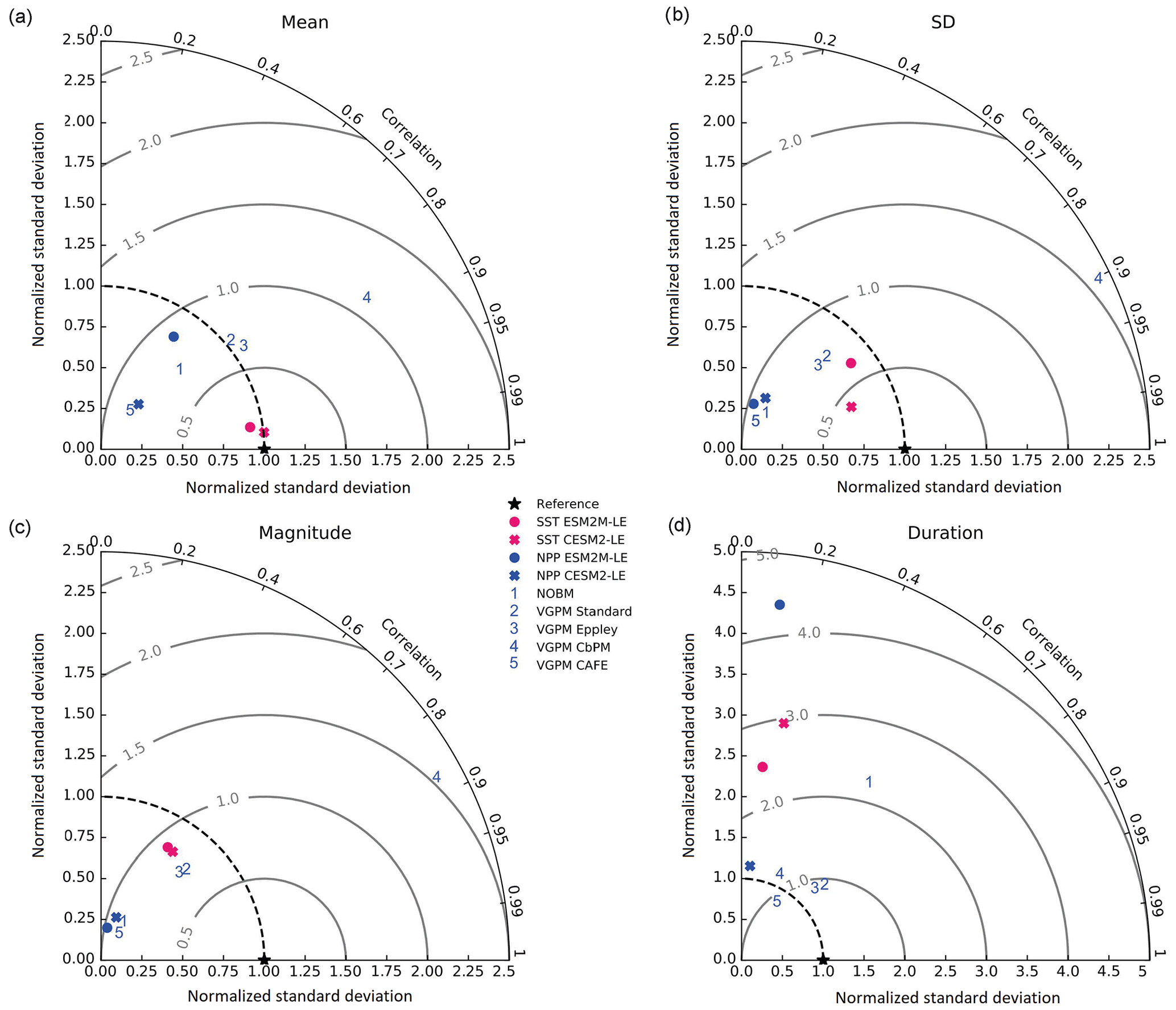
Figure 1 Comparative assessment of the simulated mean and extreme states of SST and NPP and an observed reference. These Taylor diagrams compare the spatial pattern of the climatological mean state (a) and standard deviation (b) of 5 d mean SST and NPP, as well as of the magnitude (c) and 90th percentile of the duration (d) of MHWs and NPPX events, simulated by each model to that of a reference. The reference is calculated from the observation-based SST estimate or from the mean of the five different observation-based NPP estimates, and it is indicated by a star on the diagrams. A circle; a triangle; and the numbers 1, 2, 3, 4, and 5 represent ESM2M-LE, CESM2, NOBM, Standard VGPM, Eppley-VGPM, CbPM-VGPM, and CAFE-VGPM, respectively. The Pearson correlation coefficient, which quantifies similarity between the simulated pattern and the reference, is indicated by the azimuthal angle; the centered RMSE in the simulated field is proportional to the distance from the star on the x axis; and the standard deviation of the simulated pattern is indicated by the radial distance from the origin. All statistics are normalized by the standard deviation of the reference.

The MHW magnitudes identified from the satellite-based observations are similar to those simulated by ESM2M-LE and CESM2-LE (Figs. 1c and B2a–c). However, both models simulate MHWs that last longer than those in the observations (Fig. B2d–f), especially in the eastern equatorial Pacific. This is a common bias across all current global Earth system models (Frölicher et al., 2018), irrespective of their vertical and horizontal resolution (Pilo et al., 2019). The spatial pattern of MHW duration is reasonably well simulated in both models (Fig. 1d). In contrast, the models differ in their representation of NPPX events (Figs. 1c–d and B3). The observation-based mean NPPX magnitude is most intense (< 250 mg C m⁻² d⁻¹) in the tropical Atlantic Ocean and in the northern high latitudes, whereas the magnitude is most intense in ESM2M-LE in the equatorial Pacific and in the Indian Ocean and in CESM2-LE in the northern high latitudes and in the Southern Ocean. Given the low agreement between the observation-based NPP products (Fig. 1c), it is difficult to assess how well ESM2M-LE and CESM2-LE simulate the magnitude of NPPX events and which of the two models is more realistic. We also compare the 90th percentile of the duration of NPPX events (Fig. 1d) to highlight differences between the observations and the models even though their observed and simulated median duration is close to 5 d over the global ocean due to the predominance of short NPPX events. In the observations, NPPX events reach their longest durations (> 70 d) in the central equatorial Pacific (Fig. B3d). The spatial patterns simulated by the models for the NPPX event duration differ from that of the observed reference (r < 0.2 for ESM2M-LE and for CESM2-LE, Fig. 1d). In ESM2M-LE, the longest events (> 90 d) occur within the subtropical gyres, where NPP anomalies do not vary much over time (Fig. B3e, normalized and centered RMSE = 4.3 in Fig. 1d). Longer NPPX durations in ESM2M-LE compared to observations might arise from an overestimation of durations in the non-eddying ocean models, which might fail to capture short-lived extremes associated with mesoscale and submesoscale processes. However, it might also be explained by an underestimation of durations in the observations due to gaps in satellite observations. In contrast, in CESM2-LE, events are of short duration over most of the global ocean and slightly longer (>30 d) in the high latitudes and in the eastern equatorial Pacific (Fig. B3f).

Overall, ESM2M-LE and CESM2-LE represent the mean state of and variability in SST reasonably well. Their representation of NPP diverges from observations, yet the reference for NPP observation in Fig. 1 is computed as the mean of five observation-based NPP products which themselves disagree (Fig. B1), although the spatial pattern of the mean state of and variability in NPP is broadly similar across products. Considering that both ESM2M-LE and CESM2-LE capture this spatial pattern, they appear suited to investigating the likelihood and drivers of compound MHW–NPPX events over the global ocean. However, divergent magnitudes and durations of NPPX events in ESM2M-LE and CESM2-LE hint at different drivers for NPPX events in the two models. Different processes might thus drive NPPX in association with an MHW and result in a compound MHW–NPPX event in ESM2M-LE and CESM2-LE.

2.5 Driver decomposition of compound MHW–NPPX events

We investigate the drivers of compound MHW–NPPX events and more specifically the drivers of extreme reductions in NPP during MHWs. Both ESM2M and CESM2 contain an ecological module distinguishing between three different phytoplankton types (small, large, and diazotrophs), for which specific constants and limitation terms are used to compute NPP. Total net phytoplankton production is simply the sum of NPP over all three phytoplankton types. Thus, during a low-NPP event, although the total phytoplankton NPP is extremely low, not all types may have contributed to that anomaly. We ignore the diazotrophs in this study as their contribution to total NPP (1.5 % in ESM2M-LE and 3 % in CESM2-LE on average) and to the total NPP anomaly during compound MHW–NPPX events (< 0.1 % in ESM2M-LE and CESM2-LE) is negligible. Thus, in each model, total NPP is approximated as the sum of small- and large-phytoplankton NPP.

For each phytoplankton type i, NPP is the product of its growth rate μ and its biomass n:

$$\begin{array}{}\text{(1)}& {\mathrm{NPP}}_i={\mathit{\mu }}_i{n}_i.\end{array}$$

Therefore, any anomaly in NPP, dNPP, can be decomposed as

$$\begin{array}{}\text{(2)}& {\mathrm{dNPP}}_i=n_i\mathrm{d}{\mathit{\mu }}_i+{\mathit{\mu }}_i\mathrm{d}{n}_i.\end{array}$$

If dNPP stands for the mean NPP anomaly during compound events relative to the climatological mean state of the seasonal cycle, we can assess the contributions of the mean growth anomaly, dμ, and of the mean biomass anomaly, dn, during compound events to dNPP.

TOPAZv2 and MARBL define μ in the same way:

$$\begin{array}{}\text{(3)}& {\mathit{\mu }}_i={\mathit{\mu }}_{{max}_i}{T}_{{\mathrm{f}}_i}{L}_{{\lim }_i}{N}_{{\lim }_i},\end{array}$$

where T_f is a function of the temperature, L_lim is the light limitation, and the nutrient limitation N_lim is computed using Liebig’s law of the minimum. More details are provided in Appendix A. Both N_lim and L_lim are between 0 and 1, where 1 means they do not limit phytoplankton growth and 0 means they fully suppress growth. Figure B4 in the Appendix presents the climatological mean states of T_f, L_lim, and N_lim.

dμ can be decomposed into the contributions of a change in T_f, L_lim, and N_lim during compound events.

$$\begin{array}{}\text{(4)}& \begin{array}{rl}\mathrm{d}{\mathit{\mu }}_i& ={\mathit{\mu }}_{{max}_i}\left(N_{{\lim }_i}{L}_{{\lim }_i}\mathrm{d}{T}_{{\mathrm{f}}_i}+N_{{\lim }_i}{T}_{{\mathrm{f}}_i}\mathrm{d}{L}_{{\lim }_i}\right.\\ & \left.+T_{{\mathrm{f}}_i}{L}_{{\lim }_i}\mathrm{d}{N}_{{\lim }_i}\right)\end{array}\end{array}$$

This decomposition enables us to assess the drivers of a change in phytoplankton growth during compound events. Drivers of a change in phytoplankton biomass n are less trivial as n depends on NPP itself. In TOPAZv2 and MARBL, n is considered a tracer whose time derivative is defined as follows:

$$\begin{array}{}\text{(5)}& {\partial }_t{n}_i={\mathrm{NPP}}_i-{\mathrm{Loss}}_i+{\mathrm{Circ}}_i,\end{array}$$

where NPP and Loss are the biological production and decay of phytoplankton, respectively, and Circ corresponds to the physical advection and mixing of phytoplankton by ocean circulation. The model equations only hold at the time and vertical resolution of model computations, i.e., at 2 h and 10 m resolution. Here we use 5 d mean output and data averaged over the top 100 m layer. Therefore, Eq. (5) becomes

$$\begin{array}{}\text{(6)}& {\partial }_t{n}_i={\mathrm{NPP}}_i-{\mathrm{Loss}}_i+{\mathrm{Circ}}_i+{\mathrm{Errors}}_i.\end{array}$$

Given that we do not have the necessary output to compute the circulation term, we cannot assess how small Errors is, and therefore we cannot neglect it.

Over time, biomass changes build up a biomass anomaly dn that might be sufficient to drive or contribute to driving extremely low dNPP. In this study, we intend to explain the contribution of dn to dNPP during compound MHW–NPPX events using Eq. (6). A positive or negative biomass anomaly during a compound event may be explained by an overall increase or decrease in biomass over time, until the largest biomass anomaly reached during the compound event. Therefore, we integrate ∂_tn, NPP, and Loss over all periods over which dn builds up, i.e., over which n changes from its climatological mean value (at t₀, n_i(t₀)=0) to its maximum absolute anomaly relative to the climatology reached during a compound event (at t_max, $n_i\left(t_{max}\right)=n_{imax}$). Δn refers to the integrated biomass change between t₀ and t_max, which corresponds to the largest biomass anomaly reached during a compound event. Note that Δn is not exactly equivalent to dn. Δn is a tool to understand the buildup of the largest biomass anomaly reached during a compound event, whereas dn is the mean biomass anomaly over all compound-event days.

$$\begin{array}{}\text{(7)}& {\displaystyle }\begin{array}{rl}\mathrm{\Delta }{n}_i& =\underset{t_{\mathrm{0}}}{\overset{t_{max}}{\int }}{\partial }_t{n}_i\mathrm{d}t=\underset{t_{\mathrm{0}}}{\overset{t_{max}}{\int }}({\mathrm{NPP}}_i-{\mathrm{Loss}}_i)\mathrm{d}t\\ & +\underset{t_{\mathrm{0}}}{\overset{t_{max}}{\int }}({\mathrm{Circ}}_i+{\mathrm{Errors}}_i)\mathrm{d}t\end{array}\text{(8)}& {\displaystyle }\mathrm{\Delta }{n}_i=\underset{t_{\mathrm{0}}}{\overset{t_{max}}{\int }}{\partial }_t{n}_i\mathrm{d}t=\underset{t_{\mathrm{0}}}{\overset{t_{max}}{\int }}({\mathrm{NPP}}_i-{\mathrm{Loss}}_i)\mathrm{d}t+{\mathrm{Residual}}_i\end{array}$$

The term ${\int }_{t_{\mathrm{0}}}^{t_{max}}({\mathrm{NPP}}_i-{\mathrm{Loss}}_i)\mathrm{d}t$ accounts for the contribution of biological processes to Δn, whereas Residual includes both the contribution of ocean circulation to Δn and all errors inherent to the decomposition using 5 d mean and vertically integrated output. Results are averaged over all compound events. In theory, this method could enable us to apprehend the contribution of biological processes to dn. However, errors in the decomposition might be substantial and result in a poor estimation of that contribution. Further work with more highly temporally and spatially resolved model output is needed to fully decompose the biomass changes during compound MHW–NPPX events into its drivers.

Details on the computation of phytoplankton loss are provided in Sect. A1.5 for TOPAZv2 and Sect. A2.5 for MARBL, and Fig. B5 presents the climatological mean states of NPP, Loss, n, and μ.

3 Results

3.1 Hotspots of compound MHW–NPPX events in the global ocean

Figure 2 shows the present-day distribution of compound MHW–NPPX events. Under the assumption of independence between MHW and NPPX events, the expected frequency of compound MHW–NPPX events is 1 % of time intervals or 3.65 d yr⁻¹ over the global ocean (Sect. 2.3). However, observation-based estimates show strong regional deviations from this expected frequency (Fig. 2a). Most compound events occur in the low latitudes, with hotspots of especially high frequency in the center of the equatorial Pacific, in the subtropical Indian Ocean, and around Antarctica. In these regions, compound MHW–NPPX events occur more than 3 times more frequently (> 3 % or > 10 d yr⁻¹) than would be expected if univariate extremes were independent. Compound MHW–NPPX events are also relatively frequent (about 2 % or 7 d yr⁻¹) in the low to middle latitudes between 10 and 45^∘. In contrast, compound events are rare (about 0.5 % or 2 d yr⁻¹) in the high northern latitudes north of 45^∘ N and between 45 and 60^∘ S in the Southern Ocean. However, these estimates correspond to the mean of the results obtained from five observation-based NPP products, which disagree particularly in the high southern latitudes and somewhat in the low latitudes (Figs. 2d and B6). Around Antarctica, the frequency computed using NOBM's NPP is much lower on average (0.5 %) than those computed using VGPM-based NPP products (> 4 %). Sea ice and clouds create gaps in the satellite ocean color data that are potentially more extended in time and space around Antarctica than over the rest of the global ocean. Sparse satellite data coverage implies that in NOBM, fewer ocean color observations are available to constrain NPP estimates, whereas in VGPM-based models, gaps are filled by interpolation with data points that might be too distant in space and time to yield a realistic estimate of NPP (Rousseaux and Gregg, 2014; http://orca.science.oregonstate.edu/gap_fill.php, last access: 21 October 2021). For this reason, we have lower confidence in the NOBM and VGPM-based NPP products around Antarctica than elsewhere. In the low to middle latitudes, the frequency computed using Standard VGPM is higher than that of all other observation-based estimates (Fig. 2d). Standard VGPM is the only model that uses a polynomial function to describe the temperature dependence of photosynthesis. Therefore, extremely hot surface waters in the warm low to middle latitudes have a weaker positive effect on photosynthesis and thus on NPP in Standard VGPM than in the other observation-based products. It may thereby be easier for high SST to co-occur with low NPP, resulting in higher frequency of compound MHW–NPPX events in Standard VGPM in the low to middle latitudes.

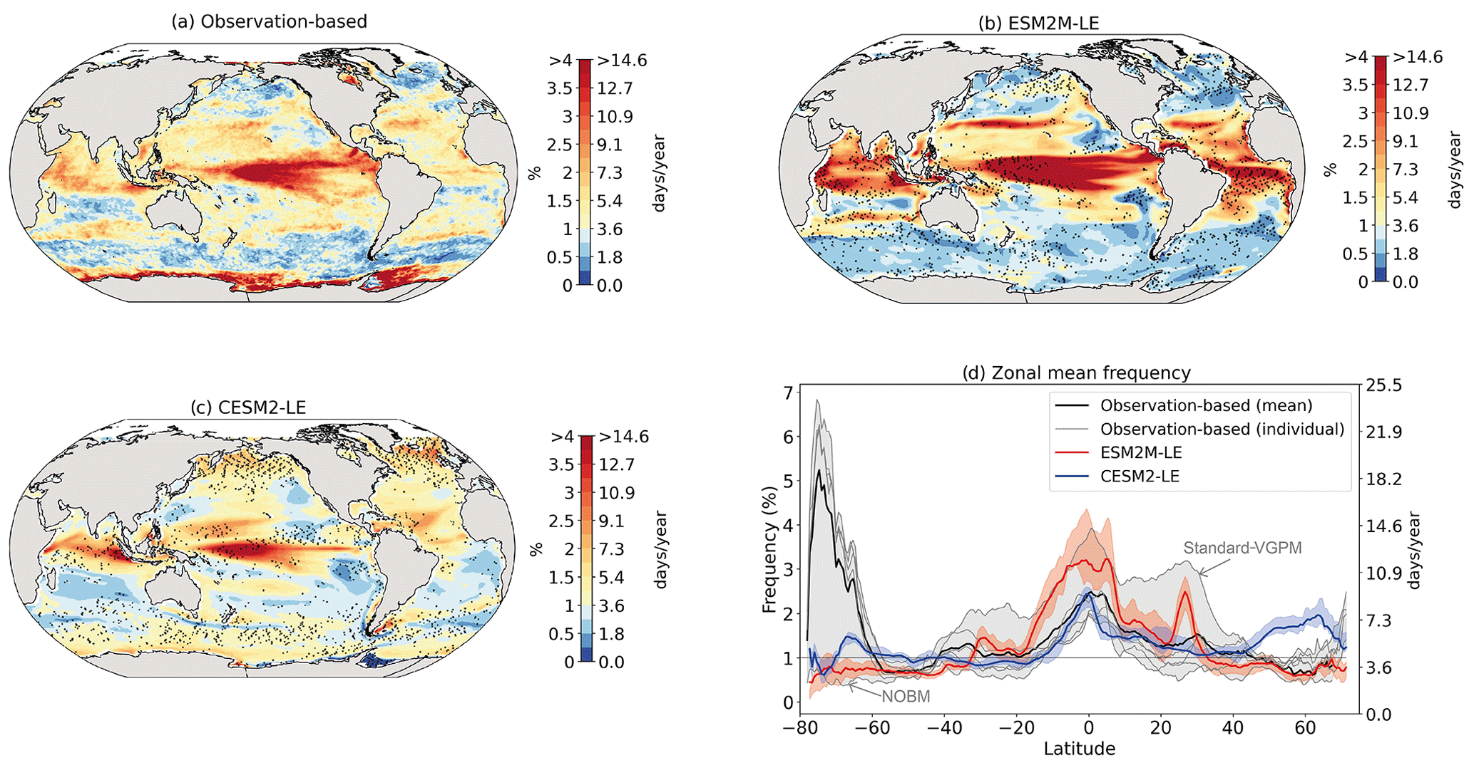
Figure 2 Frequency of compound MHW–NPPX events in (a) observation-based estimates and as simulated by (b) ESM2M-LE and (c) CESM2-LE. Observations correspond to the mean of the results obtained with five satellite-based estimates of NPP, namely NOBM, Standard VGPM, Eppley-VGPM, CbPM-VGPM, and CAFE-VGPM. (d) Zonal mean frequency of compound MHW–NPPX events. The gray-, red-, and blue-shaded areas in (d) indicate the range of the observation-based estimates, of the ESM2M-LE members, and of the CESM2-LE members, respectively. Stippling in (b) and (c) corresponds to regions where the frequency simulated by ESM2M-LE and CESM2-LE is outside the range of the observation-based estimates, i.e., higher or lower than all five observation-based estimates.

Next, we compare the simulated frequency of compound MHW–NPPX events in ESM2M-LE (Fig. 2b) and CESM2-LE (Fig. 2c) to the observation-based frequency (Fig. 2a, d). Overall, the simulated frequency pattern is similar in the two models and mostly within the uncertainty range of the observational products (e.g., areas with no stippling in Fig. 2b and c, corresponding to 84 % of the global ocean in ESM2M-LE and to 82 % in CESM2-LE). The models correctly simulate frequent compound MHW–NPPX events in the equatorial Pacific (> 4 % or > 14 d yr⁻¹) and relatively frequent compound events in the low to middle latitudes between 10 and 45^∘ (2 % or 7 d yr⁻¹; Fig. 2a–c). ESM2M-LE simulates too frequent compound events in the southern tropical Atlantic, in the center of the equatorial Pacific, and in the northern part of the Indian Ocean. CESM2-LE simulates too frequent compound events in the western equatorial Pacific and in the northern part of the Indian Ocean. In spite of there being relatively few dissimilarities between models and observations in the low and middle latitudes, they strongly disagree in the high latitudes. ESM2M-LE slightly outperforms CESM2-LE, especially in the northern high latitudes, where it simulates rare compound events consistent with the observation-based estimates, whereas CESM2-LE simulates too frequent compound events (> 1 %). Around Antarctica, neither ESM2M-LE nor CESM2-LE simulates the very frequent compound MHW–NPPX events shown in the observations. However, low agreement between the five observation-based estimates (their frequency being as low as 0.5 % and as high as 6.5 % on average at 75^∘ S, in Fig. 2d) makes it difficult to determine which of the two models better simulates compound events in this regions.

3.2 Small- and large-phytoplankton NPP anomalies during compound MHW–NPPX events

Next, we assess which phytoplankton type is responsible for NPPX during compound MHW–NPPX events. In both models, total NPP is approximately equal to the sum of small- and large-phytoplankton NPP (Sect. 2.5), whose respective mean anomalies (relative to the mean seasonal cycle) during compound MHW–NPPX events are presented in Fig. 3a–d.

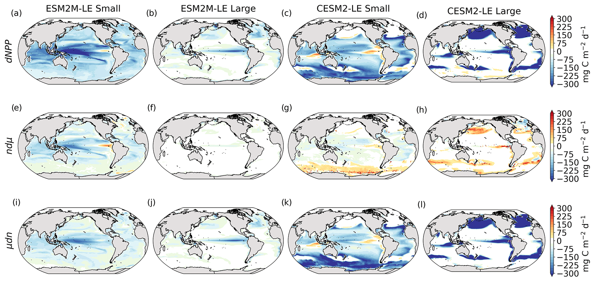
Figure 3 Small- and large-phytoplankton NPP anomalies, dNPP, relative to the climatological seasonal cycle (mg C m⁻² d⁻¹) during compound MHW–NPPX events in ESM2M-LE (a, b) and in CESM2-LE (c, d) and contributions of the growth rate ndμ (e–h) and of the biomass anomaly μdn (i–l) to these NPP anomalies. Contours on panels (a)–(d) indicate the climatological mean state of small and large NPP averaged over 1998–2018 (see also Fig. B5a–d); labels have been omitted.

The decrease in small-phytoplankton NPP dominates the overall decrease in NPP during compound MHW–NPPX events in both models, although the models differ in the magnitude and spatial pattern of anomalies in small and large phytoplankton. The decrease in small-phytoplankton NPP accounts for 79 % and 70 % of the total NPPX anomalies in the global ocean during MHW–NPPX events in ESM2M-LE and CESM2-LE, respectively (Fig. 3a, c). Especially pronounced is the dominance of small-phytoplankton NPP decreases in the low to middle latitudes and the Southern Ocean in both models. This implies a shift in the phytoplankton community composition from small phytoplankton towards more large phytoplankton during MHW–NPPX events in these regions, with potential repercussions for marine community structure. In both models, decreases in large-phytoplankton NPP dominate the NPP decrease during MHW–NPPX events in the eastern equatorial Pacific. Large-phytoplankton NPP also decreases during MHW–NPPX events in the northern high latitudes. In CESM2-LE, the decline in large-phytoplankton NPP even dominates the response in the northern high latitudes as small-phytoplankton NPP increases, resulting in an assemblage shift towards smaller phytoplankton there. In addition, the decline in large-phytoplankton NPP also dominates along the southern boundaries of the subtropical gyres in the Southern Hemisphere in CESM2-LE. Overall, these patterns resemble well the climatological mean state pattern of small- and large-phytoplankton NPP (Figs. 3a–d and B5a–d). Small-phytoplankton anomalies during MHW–NPPX events dominate in regions where the climatological mean state of small-phytoplankton NPP generally dominates, whereas large-phytoplankton NPP anomalies play an important role during MHW–NPPX events where the climatological mean state of large-phytoplankton NPP generally dominates.

3.3 Drivers of low NPP during compound MHW–NPPX events

To understand the drivers of NPPX during compound MHW–NPPX events, we decompose the NPP anomaly dNPP of each phytoplankton type into the contributions of its growth rate anomaly dμ (Fig. 3e–h) and of its biomass anomaly dn (Fig. 3i–l) (see Eq. 2 in Sect. 2.5). One must note, however, that these variables are not independent and that the biomass anomaly may result from changes in the growth rate itself. The decomposition amounts to 104 % and 105 % of the global dNPP of small and large phytoplankton, respectively, in ESM2M-LE and to 104 % and 99 % of the global dNPP of small and large phytoplankton, respectively, in CESM2-LE (Fig. B7). Our decomposition method is therefore well suited to investigating the drivers of extreme reductions in NPP during MHW–NPPX events.

Globally, the growth rate anomaly dμ barely contributes to the large-phytoplankton dNPP in ESM2M-LE (28 %, Fig. 3b, f) and to the small- and large-phytoplankton dNPP in CESM2-LE (−12 % and −14 %, respectively; Fig. 3c, d, g, h). A large part of the extreme reduction in NPP during MHWs is in fact driven by a negative biomass anomaly dn in both models and for both phytoplankton types. However, the growth rate anomaly explains about half (51 %) of the global small-phytoplankton dNPP in ESM2M-LE (Fig. 3a, e) and can regionally be even more dominant. In ESM2M-LE, the contribution of dμ (i.e., ndμ) is most negative in the low latitudes for small phytoplankton (Fig. 3e), especially in the western equatorial Pacific. In CESM2-LE, the contribution of dμ is slightly negative in the low latitudes (Fig. 3g), and positive (i.e., it counteracts the negative dNPP) in the high latitudes and eastern equatorial Pacific for small and large phytoplankton (Fig. 3g, h). In other words, an increase in the growth rate increases small- and large-phytoplankton NPP in these regions in CESM2-LE. However, the large decreases in dn overcompensate for this increase in the growth rate and lead to an overall decrease in NPP for small phytoplankton in the low to middle latitudes and in the high southern latitudes (Fig. 3k) and for large phytoplankton in the eastern equatorial Pacific, in the high northern latitudes, and at around 40^∘ S (Fig. 3l).

Increases in small- or large-phytoplankton NPP moderate the negative dNPP during MHW–NPPX events. In ESM2M-LE, small-phytoplankton NPP locally increases in the eastern equatorial Pacific as a result of increased small-phytoplankton growth (Fig. 3e). In CESM2-LE, the increase in small-phytoplankton NPP in the northern high latitudes and the increase in large-phytoplankton NPP in the southern high latitudes are driven by both an increase in growth and an increase in biomass (Fig. 3g, h, k, l).

3.3.1 Phytoplankton growth rate anomaly during compound MHW–NPPX events

Before explaining the changes in phytoplankton biomass, we look into the drivers of changes in phytoplankton growth rates because they contribute to reducing NPP either directly or indirectly by affecting phytoplankton biomass. Figure 4 shows the spatial pattern of the mean growth rate anomaly dμ during compound events for small and large phytoplankton in each model, as well as the contributions of temperature, light and nutrient limitations to dμ, as described in Sect. 2.5.

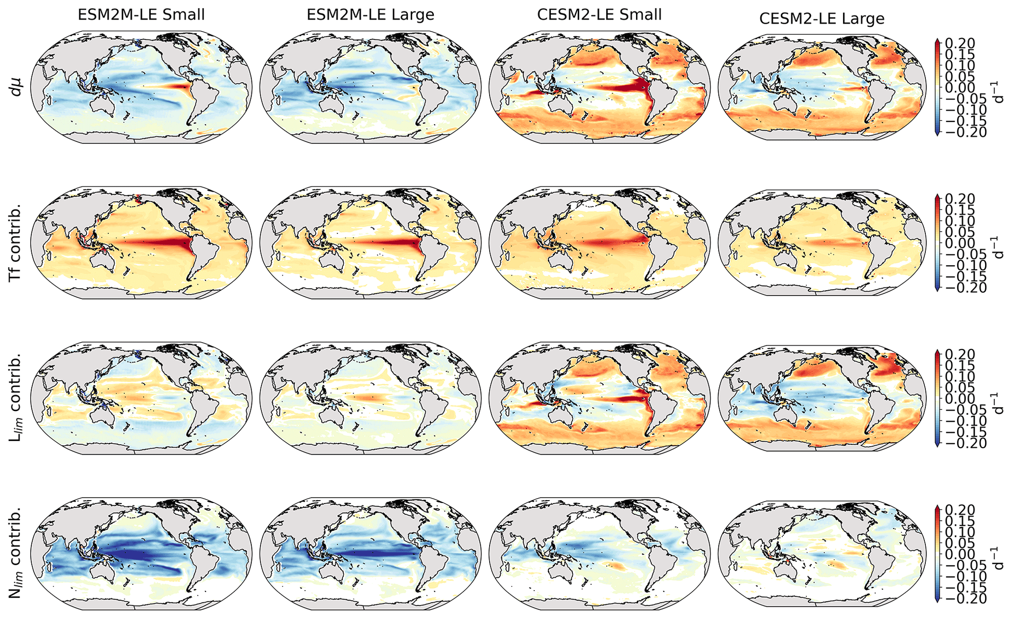
Figure 4 Growth rate anomaly dμ (d⁻¹) of small and large phytoplankton during compound MHW–NPPX events in ESM2M-LE (a, b) and in CESM2-LE (c, d) and contributions of a change in the temperature function T_f (e–h), in the light limitation L_lim (i–l), and in the nutrient limitation N_lim (m–p) to this growth rate anomaly. The decomposition of dμ into these three contributions comes with a global mean residual of 0.009 and −0.002 d⁻¹ for small and large phytoplankton in ESM2M-LE and of −0.007 and 0.002 d⁻¹ for small and large phytoplankton in CESM2-LE.

In ESM2M-LE, the drivers of dμ are similar during compound events for small and large phytoplankton. The negative growth rate anomaly in the low to middle latitudes (Fig. 4a, b) is associated with increased nutrient limitation (−0.10 d⁻¹ on average between 40^∘ S and 35^∘ N; Fig. 4m, n), i.e., reduced mixing of nutrient-rich waters from the deeper ocean to the upper 100 m. In the high latitudes, the negative growth rate anomaly is mainly associated with increased light limitation (−0.05 d⁻¹ on average south of 40^∘ S and north of 35^∘ N; Fig. 4i, j). Even though the light limitation depends on a number of factors other than the light supply, such as temperature, nutrient levels, mixed-layer depth, or the carbon-to-chlorophyll ratio in phytoplankton, increased light limitation is here a direct result of reduced light supply by −13 W m⁻² on average (Fig. B8a). High-latitude MHWs are, however, mainly driven by enhanced shortwave radiation in summer (Vogt et al., 2022). Enhanced shortwave radiation seems incompatible with reduced light levels, hence the low compound MHW–NPPX event frequency in the high latitudes in ESM2M-LE. Therefore, for MHWs to co-occur with reduced light levels, they must be driven by drivers other than radiative heating, such as vertical mixing or advective processes. These drivers might be compatible with clouds or extended sea-ice cover and thus with light limitation. In addition, high temperatures during MHWs also raise energy demand on phytoplankton and directly enhance the light limitation (see the role of T_f in Sect. A1.3 and A2.3). High temperatures during MHWs somewhat moderate the negative growth rate anomalies by their positive effect on the growth rate for both large and small phytoplankton, especially in the low latitudes (Fig. 4e, f). In the eastern equatorial Pacific, this positive effect of the temperature is able to overcompensate for the negative effect of nutrient limitation on the growth rate of small phytoplankton (Fig. 4e), resulting in increased small-phytoplankton growth and a shift towards small phytoplankton during MHW–NPPX events (Fig. 3a, b).

In CESM2-LE, dμ is negative in the low latitudes (Fig. 4c, d) for both small and large phytoplankton. The growth of small phytoplankton is mainly reduced by increased nutrient limitation (−0.05 d⁻¹ on average between 15^∘ S and 20^∘ N; Fig. 4o, p), whereas the growth of large phytoplankton is mainly reduced by light limitation in the low latitudes (−0.03 d⁻¹ on average between 20^∘ S and 20^∘ N; Fig. 4l). Divergent responses of the nutrient limitation to changes in nutrient levels during compound MHW–NPPX events for small and large phytoplankton can be explained by smaller half-saturation constants in small phytoplankton, which, given the formulation of the nutrient limitation in MARBL (Sect. A2.2), would result in a stronger decrease in N_lim given a certain decrease in nutrient levels. In the high latitudes, increased light levels by 7 W m⁻² on average reduce light limitation (Fig. B8b), which ultimately enhances small- and large-phytoplankton growth. High temperature anomalies contribute positively to the growth rate of small and large phytoplankton, especially in the eastern equatorial Pacific for small phytoplankton (> 0.09 d⁻¹; Fig. 4g), resulting in a shift towards large phytoplankton during MHW–NPPX events there (Fig. 3c, d).

In both models, nutrient limitation on phytoplankton growth is especially strong during MHW–NPPX events compared to simple NPPX events (not shown here). Stronger nutrient limitation all over the ocean counteracts the positive temperature effect on phytoplankton growth associated with MHWs. Overall, the models agree that phytoplankton growth is enhanced by high temperatures and reduced by low nutrient levels during MHW–NPPX events. However, the models disagree on the strength of the nutrient limitation, especially in the low latitudes and the eastern equatorial Pacific, potentially due to a stronger reduction in nutrient levels in ESM2M-LE compared to CESM2-LE. Background nutrient limitation is also higher in ESM2M-LE compared to CESM2-LE (Fig. B4i–l) and therefore more sensitive to changes in nutrient levels (see the formulation of N_lim in Sect. A1.2 and A2.2). Lastly, the models disagree on their representation of the light limitation changes during MHW–NPPX events, especially in the high latitudes. This model divergence may arise from a number of factors involved in the calculation of L_lim, such as different light harvest coefficients in TOPAZv2 (Sect. A1.3) and MARBL (Sect. A2.3), but most importantly, divergent representation of the coupling between radiative fluxes, ocean temperature, and phytoplankton growth in the two models results in different light levels during MHW–NPPX events.

3.3.2 Phytoplankton biomass anomaly during compound MHW–NPPX events

Next, we investigate the drivers of the mean phytoplankton biomass anomaly dn during compound MHW–NPPX events (Fig. 5a–d), which contributes to driving dNPP. The spatial pattern of dn resembles the spatial pattern of dNPP (Fig. 3a–d); their Pearson's correlation coefficients are 0.4 and 0.9 for small and large phytoplankton, respectively, in ESM2M and 0.8 and 0.9 for small and large phytoplankton, respectively, in CESM2. In ESM2M-LE, the negative dn is rather uniform across latitudes for small phytoplankton (Fig. 5a) but shows a distinct spatial pattern for large phytoplankton with stronger declines in the eastern equatorial Pacific and in the high northern latitudes (Fig. 5b). In CESM2-LE, low NPP is driven by a decrease in small-phytoplankton biomass in the southern high latitudes and partly in the low latitudes (Fig. 5c) and by a decrease in large-phytoplankton biomass along the Equator, in the northern high latitudes, and in the southern boundary of the subtropical gyres of the Southern Hemisphere (Fig. 5d).

Figure 5 Biomass anomaly dn (mg C m⁻²) of small and large phytoplankton during compound MHW–NPPX events in ESM2M-LE (a, b) and in CESM2-LE (c, d). Integrated biomass change Δn (mg C m⁻²) leading to the maximum anomaly reached during a compound MHW–NPPX event (e–h). Contribution of biological processes (NPP−Loss, i–l) to Δn.

We are further interested in the buildup of this biomass anomaly dn over time. Δn is the integrated biomass change over the period over which biomass anomalies build up (Sect. 2.5). Even though dn and Δn differ by definition, they have almost identical spatial patterns (Fig. 5a–d compared to Fig. 5e–h), signifying it is indeed possible to understand dn from Δn.

Δn is driven by changes in the difference between phytoplankton NPP and Loss (NPP − Loss; Fig. 5i–l) and by changes in ocean circulation (see Eq. 8). The residual presented in Fig. B10 includes both the unknown contribution of ocean circulation and all errors inherent to our decomposition at low temporal resolution and vertical integration.

The role of biological processes in driving dn can be apprehended by the sign of the integrated NPP − Loss term over the period over which dn builds up. Although the individually integrated NPP and Loss terms seem almost equivalent (Fig. B9), phytoplankton loss actually exceeds phytoplankton NPP over most of the global ocean (Fig. 5i–l), which might contribute to decreasing the biomass over time (Fig. 5e–h) and thus to driving the negative biomass anomaly dn (Fig. 5a–d).

In ESM2M-LE, integrated NPP − Loss is particularly negative (< −150 mg C m⁻²) for small phytoplankton in the low to middle latitudes between 35^∘ S and 35^∘ N and for large phytoplankton in the northern high latitudes and in a narrow band along the Equator (Fig. 5i, j). In CESM2-LE, the negative NPP − Loss contribution to Δn seems especially strong (< −200 mg C m⁻²) for small phytoplankton in the low to middle latitudes between 35^∘ S and 35^∘ N and in the Southern Ocean and for large phytoplankton along the Equator and in the high latitudes (Fig. 5k, l).

Note that integrated NPP − Loss generally exceeds the integrated biomass changes (Fig. 5e–l), with some exceptions, e.g., in the high latitudes for small phytoplankton in ESM2M-LE. Δn, NPP, and Loss terms include an error term when computed from 5 d mean, 10 m vertically integrated biomass. Further studies at higher temporal and vertical resolution are needed to remove errors in all terms in Eq. (8) so as to quantify the exact NPP − Loss contribution to Δn.

Overall in both models, the negative biomass anomaly dn (Fig. 5a–d) can be explained by negative biomass changes (Δn, Fig. 5e–h) over time, which seem to be driven by negative contributions from NPP − Loss (Fig. 5m–p). Loss terms include grazing of phytoplankton by zooplankton in TOPAZv2 and by grazing, mortality, and aggregation in MARBL. During MHWs, not only do higher temperatures enhance NPP via their positive effect on the growth rate but they also directly enhance phytoplankton loss via their similarly positive effect on phytoplankton grazing and mortality (see Sect. A1.5 and A2.5). However, other factors such as nutrient and light limitation moderate phytoplankton growth during compound MHW–NPPX events, as we have seen in the previous section. In turn, nutrient and/or light limitation might moderate NPP sufficiently for it to be exceeded by phytoplankton loss, allowing a decrease in phytoplankton biomass over time.

3.3.3 Summary of driving processes

Figure 6 summarizes the drivers of NPPX during MHWs in ESM2M-LE and in CESM2-LE. We distinguish between four regions of rather homogeneous drivers: the northern high latitudes north of 35^∘ N; the low latitudes between 35^∘ S and 35^∘ N, except for the eastern equatorial Pacific (as defined by Fay and Mckinley, 2014); and lastly the southern high latitudes south of 35^∘ S. Small- and large-phytoplankton contributions to dNPP are represented in Fig. 6 by dark and light colors, respectively. Here, we compare the drivers of NPPX in the two models and choose not to focus on the magnitude of their NPP anomalies (note the different y axes in Fig. 6). Small and large phytoplankton both contribute to driving NPPX during compound MHW–NPPX events. In the two models, small phytoplankton is responsible for the majority (> 70 %) of dNPP in the low latitudes and in the southern high latitudes. In ESM2M, large phytoplankton accounts for a larger part (44 %) of dNPP in the northern high latitudes and about half of dNPP over the cold tongue, whereas in CESM2-LE, large phytoplankton dominates (> 84 %) dNPP in the northern high latitudes and over the cold tongue.

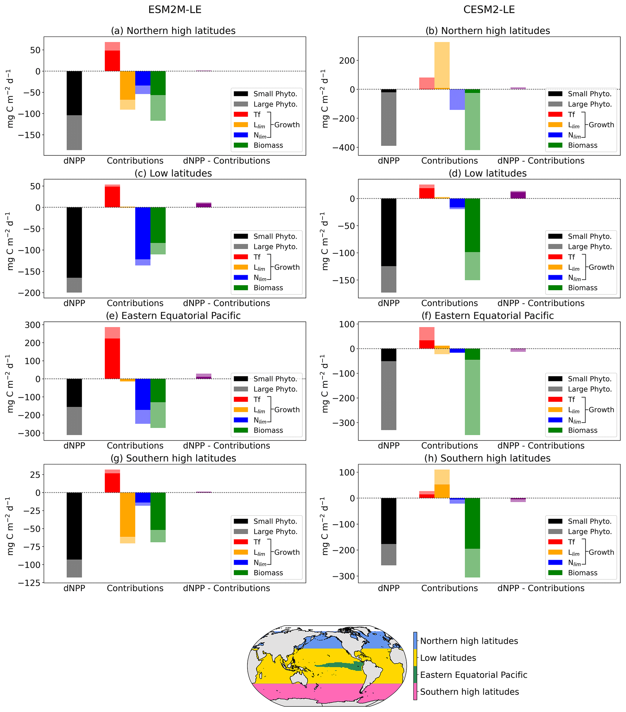
Figure 6 Regional mean NPP anomaly (mg C m⁻² d⁻¹) during compound MHW–NPPX events in ESM2M-LE and in CESM2-LE over the northern latitudes (a, b), the low latitudes (c, d), the eastern equatorial region (e, f), and the southern latitudes (g, h). Contributions of the small- and large-phytoplankton dNPP to the total NPP anomaly are represented in black and gray, respectively. The indirect contributions to dNPP of changes in each phytoplankton growth limiting factor (the temperature function T_f, in red; the light limitation L_lim, in orange; and the nutrient limitation N_lim, in blue) and of changes in phytoplankton biomass, in green, during compound MHW–NPPX events are indicated in dark and light colors for small and large phytoplankton, respectively. Remaining changes in NPP that could not be explained by the decomposition of dNPP are represented in purple.

We further decomposed dNPP into the contributions from a change in the temperature function T_f (red bars in Fig. 6), in the light limitation L_lim (yellow bars), and in the nutrient limitation N_lim (blue bars) by multiplying their contributions to the growth rate anomaly dμ (Sect. 3.3.1) with the climatological mean biomass n. We also assessed the contribution of the biomass anomaly dn (green bar) to dNPP by multiplying dn with the climatological mean growth rate μ (Sect. 3.3.2). In Fig. 6, we did not decompose the biomass anomaly contribution to dNPP into the further contribution of a change in NPP−Loss, since this decomposition might be associated with substantial errors when performed at 5 d mean resolution and when integrating over the top 100 m layer (see Sect. 2.5), resulting in a slightly inaccurate estimation of the NPP−Loss contribution. The decomposition in Sect. 3.3.2 is not intended to quantify the exact NPP−Loss contribution to dn but rather to apprehend the sign of the biomass anomaly.

Over all four regions and in both models, high temperatures during MHWs have a positive effect on the growth rate and thus positively contribute to dNPP. This positive effect can be supported or counteracted by the light and nutrient contributions to dNPP.

On average, in the low latitudes, changes in the light limitation hardly contribute to dNPP. In the high latitudes and in the equatorial Pacific, the models disagree on the sign of the light contribution. Although in CESM2-LE, reduced light limitation during MHW–NPPX events has for the most part a positive effect on dNPP except on large phytoplankton in the equatorial Pacific (Fig. 6b, f, h), in ESM2M-LE, strong light limitation on phytoplankton growth contributes to reducing dNPP and thus to driving NPPX in the high latitudes (Fig. 6a, g).

The models agree that lower nutrient levels limit phytoplankton growth during compound MHW–NPPX events. However, the models disagree on the strength of the nutrient limitation changes. In ESM2M-LE, the nutrient limitation on phytoplankton growth is strong enough (in combination with the light limitation in the high latitudes) to reduce the growth rate, which directly contributes to reducing NPP and thus to driving NPPX events (Fig. 6a, c, e, g). On the other hand, in CESM2-LE, the nutrient limitation is not sufficient to counterbalance the positive effects of temperature and light on the growth rate during MHWs in the high latitudes and over the cold tongue (Fig. 6b, d, h) and only slightly contributes to reducing dNPP in the low latitudes (Fig. 6f) along with enhanced light limitation.

Both models agree on low phytoplankton biomass during compounds events, which contributes to driving low NPP over all four biomes. The negative biomass anomaly might be explained by a relative increase in phytoplankton loss compared to phytoplankton NPP during compound events, as discussed in Sect. 3.3.2. It might also be explained or counteracted by changes in ocean circulation, which this study does not address. Low biomass contributes to driving NPPX by about 50 % in ESM2M-LE and > 100 % in CESM2-LE.

Overall, the models agree on the effect of high temperatures, which tend to increase NPP during MHWs. They disagree on the sign of the light limitation in the high latitudes, potentially due to reduced light levels in ESM2M-LE and higher light levels in CESM2-LE during compound MHW–NPPX events. Lastly, the models agree on increased nutrient limitation during compound MHW–NPPX events, which contributes to driving NPPX. The main difference between ESM2M-LE and CESM2-LE is the strength of the nutrient limitation effect on phytoplankton growth during MHW–NPPX events. In ESM2M-LE, the nutrient limitation is strong enough to reduce the growth rate and directly drive NPPX. In CESM2-LE, weaker nutrient limitation simply moderates the temperature effect on the growth rate and thus on NPP, thereby potentially allowing NPP to be exceeded by phytoplankton loss, which might decrease the biomass over time and eventually drive NPPX. Divergent responses of the nutrient limitation in the two models can be explained by a stronger reduction in nutrient levels during MHW–NPPX events in ESM2M-LE compared to CESM2-LE and by higher background nutrient limitation in ESM2M-LE, which implies higher sensitivity of the nutrient limitation to changes in nutrient levels.

4 Discussion and conclusion

We had three primary goals in setting out with this study: (i) identify hotspots of compound marine heatwaves and low-NPP (MHW–NPPX) events, (ii) assess the fidelity of state-of-the-art Earth system models (ESMs) in representing MHW–NPPX events, and (iii) apply the models to develop mechanistic insights into the underlying drivers of these potentially harmful compound MHW–NPPX events.

The analysis revealed that compound MHW–NPPX events occur relatively frequently in the low latitudes, especially in the center of the equatorial Pacific and in the subtropical Indian Ocean, and less frequently in the northern high latitudes (Fig. 2a, d; first goal). Both models agree with observations in the low latitudes (second goal). However, CESM2-LE overestimates the frequency of compound MHW–NPPX events in the northern high latitudes. In the southern high latitudes, elevated uncertainty in the observation-based products renders it difficult to determine which of the two models better simulates compound events. Overall, our results agree with previous studies that reported suppressed NPP during MHWs in regions with relatively low surface nutrient levels, such as the subtropical gyres (Hayashida et al., 2020; Gupta et al., 2020; Le Grix et al., 2021). Gupta et al. (2020), for example, reported low chlorophyll during an MHW in the Indian Ocean, where background nitrate concentrations are especially low. Le Grix et al. (2021) described frequent co-occurrence of MHWs and low-chlorophyll events in the center of the equatorial Pacific and in the Indian Ocean. These correspond to the regions where we found especially frequent MHW–NPPX events in the observation-based estimates and in the two models. In addition, previous studies reported elevated chlorophyll concentrations during MHWs over regions with high nutrient concentrations, such as in the northern reaches of the Southern Ocean (Hayashida et al., 2020; Gupta et al., 2020). These are regions where we also found compound events to be rare.

We then investigated the drivers of compound MHW–NPPX events and the reasons why ESM2M-LE and CESM2-LE have similar compound-event likelihoods in the low latitudes and divergent likelihoods in the high latitudes (third goal). We found that the models represent NPPX events of different magnitude and duration, which is suggestive of different drivers for NPPX events during MHWs. In both models, higher temperatures have a positive effect on NPP during MHW–NPPX events. In ESM2M-LE, this temperature effect is counteracted by enhanced nutrient limitation in the low latitudes and by enhanced light limitation in the high latitudes, which contribute to driving approximately half of the negative NPP anomaly by directly limiting phytoplankton growth. Although higher temperatures have the same enhancing effect on phytoplankton NPP and loss, nutrient and light limitation during MHW–NPPX events might decrease NPP sufficiently for it to be exceeded by phytoplankton loss over the global ocean. This relative increase in phytoplankton loss compared to NPP possibly explains the buildup of a negative biomass anomaly that contributes to driving the other half of the negative NPP anomaly during MHW–NPPX events. In CESM2-LE, nutrient limitation over the global ocean is too weak to counterbalance the positive temperature effect on phytoplankton growth, though it may moderate the growth sufficiently for NPP to be exceeded by phytoplankton loss, resulting in a biomass decrease over time. Lower biomass is the main driver of NPPX events over the global ocean in CESM2-LE. These divergent drivers of NPPX events in ESM2M-LE and CESM2-LE reflect the low degree of agreement in how ESMs represent phytoplankton growth and loss (Laufkötter et al., 2015), with this constituting a major source of uncertainties in global projections of NPP under global warming (Laufkötter et al., 2015; Frölicher et al., 2016; Kwiatkowski et al., 2020; Tagliabue et al., 2021). We expect ESMs to differ not only in their projection of NPP but also in how they simulate future changes in NPPX events and compound MHW–NPPX events, depending on how the drivers of NPPX events evolve under global warming.

These NPPX drivers may well also be responsible for the differences in the likelihood of compound MHW–NPPX events between the models. We expect MHWs to be frequently associated with increases in vertical stratification that inhibit the upward mixing of deep nutrients (Holbrook et al., 2019; Hayashida et al., 2020); therefore, in regions where nutrient limitation is the dominant NPPX driver, we would expect NPPX events to frequently co-occur with MHWs. That is indeed the case in the low latitudes, where nutrient limitation drives NPPX events in the two models via its direct effect on the growth rate (in ESM2M) and its indirect effect on NPP−Loss, which reduces the biomass (in ESM2M-LE and CESM2-LE). Previous studies have identified nutrient limitation as the main driver of negative NPP anomalies during MHWs. For example, Whitney (2015) and Le et al. (2019) found that decreased westerly winds and southward Ekman transport over the eastern part of the North Pacific transition zone reduced nutrient concentrations during the Blob and thus inhibited NPP. Compound MHW–NPPX events are also relatively frequent in CESM2-LE in the high latitudes, where nutrient limitation contributes to driving NPPX events. On the other hand, it has been shown that MHWs are associated with enhanced incident shortwave radiation in the high latitudes (Vogt et al., 2022). Therefore, in regions where light limitation drives NPPX events, we expect rare compound events, which is indeed the case in the high latitudes in ESM2M-LE.

Our analysis revealed that compound MHW–NPPX events are accompanied by shifts in phytoplankton species. The models suggest a general shift towards larger phytoplankton over most of the global ocean during MHW–NPPX events, except in the eastern equatorial Pacific in ESM2M-LE and in CESM2-LE, as well as north of 35^∘ N and between 35 and 50^∘ S in CESM2-LE, where the contribution of smaller-phytoplankton NPP increases during MHW–NPPX events. In general, the shift towards larger phytoplankton occurs over regions where small phytoplankton are dominant and vice versa. Other studies have previously documented phytoplankton shifts during MHWs (Yang et al., 2018; Wyatt et al., 2022). Wyatt et al. (2022), for example, described a relative shift towards small phytoplankton in the northeast Pacific during the 2014–2015 Blob due to a stronger response of large phytoplankton to reduced nutrient levels and a stronger response of small phytoplankton to increased light availability driven by shallower mixed layers. Small phytoplankton even increased during the Blob over the Gulf of Alaska (Wyatt et al., 2022), in agreement with CESM2-LE, which simulates increased small-phytoplankton NPP during MHW–NPPX events in the northern high latitudes (Fig. 3c). Peña et al. (2019) also found a shift towards cyanobacteria, i.e., small phytoplankton, in the northeastern Pacific during the Blob. Their results are consistent with modeling studies showing that a surface ocean with lower nutrient concentrations and increased light availability favors smaller phytoplankton species (Litchman et al., 2006; Acevedo-Trejos et al., 2014). These phytoplankton shifts might lead to cascading impacts on marine ecosystems depending on which phytoplankton type marine species preferentially graze on (Cavole et al., 2016; Bindoff et al., 2019; Cheung and Frölicher, 2020). They might also impact the biological carbon pump because larger and heavier phytoplankton sink faster to the deep ocean (Boyd and Harrison, 1999). To better predict phytoplankton shifts and their impacts on marine ecosystems and the carbon pump during MHW–NPPX events, we need models to accurately simulate these events and their associated changes in small- and large-phytoplankton NPP. Yet models such as ESM2M and CESM2 still disagree, especially in the high latitudes.

One important aspect of our study is the use of large-ensemble simulations (LES) with high-frequency ocean output, encompassing not only SST and NPP but also diagnostic variables used for driver attribution. The large sample size mandated by the study of compound extreme events is even larger than that required for extreme events with single variables (Deser et al., 2020; Burger et al., 2022; Zscheischler and Lehner, 2022). This is particularly important under non-stationary conditions, where relatively short time series need to be analyzed to obtain a picture of quasi-stationary conditions. The application of two different Earth system models facilitated an exploration of how uncertainties in the formulation of NPP manifest themselves in the occurrence (pattern and frequency) of compound events. This should complement work by Kwiatkowski et al. (2020) and Bopp et al. (2022) in underscoring the challenges faced by the Earth system modeling community given pervasive NPP uncertainty.

One challenging aspect of our study is the lack of agreement between observation-based estimates of the frequency of compound MHW–NPPX events in the middle to high southern latitudes, which makes it difficult to determine whether the ESMs well represent compound MHW–NPPX events and their drivers over this region. NPP estimates produced by models assimilating satellite data are still uncertain and highly sensitive to their respective model configurations (e.g., Behrenfeld et al., 2005; J. S. Long et al., 2021), especially in sea-ice-covered regions. We decided to include five observation-based NPP products in this study to take into account the high uncertainty in NPP estimates, which affects the observation-based estimates of MHW–NPPX event frequency. Direct NPP measurements would be needed to better constrain the NPP estimated by ESMs in the future.

To conclude, the combination of an MHW and an NPPX event constitutes a compound hazard which potentially leads to severe impacts on marine organisms and ecosystems. Here, we assessed whether LES from two ESMs can be used to understand compound MHW–NPPX events in the ocean and to project them into the future. Our analysis reveals that the likelihood of compound MHW–NPPX events depends on how ESMs represent the factors limiting phytoplankton growth and loss. These factors are similar in ESM2M and CESM2 in the low latitudes but differ in the high latitudes. This identifies an important need for improved process understanding in the models used for predicting and projecting the potentially harmful compound MHW–NPPX events in the ocean.

Appendix A: Ecosystem model description

A1 GFDL ESM2M: TOPAZv2

TOPAZv2 stands for Tracers of Ocean Phytoplankton with Allometric Zooplankton version 2.0. It is the biogeochemical and ecological module used in GFDL's ESM2M (Dunne et al., 2013). Three phytoplankton types are represented: nano-phytoplankton (or small phytoplankton), large phytoplankton, and diazotrophs. Nitrogen in each phytoplankton type i is a prognostic variable.

$$\begin{array}{}\text{(A1)}& {\partial }_t{n}_i={\mathrm{NPP}}_i-{\mathrm{Loss}}_i+{\mathrm{Circ}}_i,\end{array}$$

where NPP is the nitrogen-specific NPP, Loss is the nitrogen-specific decay, and Circ corresponds to the physical advection and mixing of phytoplankton nitrogen n by ocean circulation. The NPP of each phytoplankton type is the product of its growth rate μ and its biomass n:

$$\begin{array}{}\text{(A2)}& {\mathrm{NPP}}_i={\mathit{\mu }}_i{n}_i.\end{array}$$

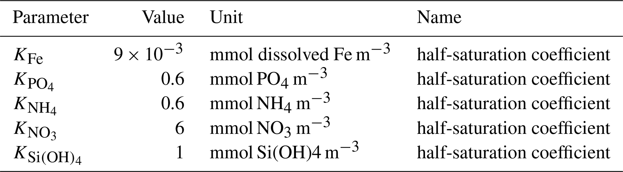
Table A1 Parameter values used in TOPAZv2 to compute the production and grazing of both small and large phytoplankton.

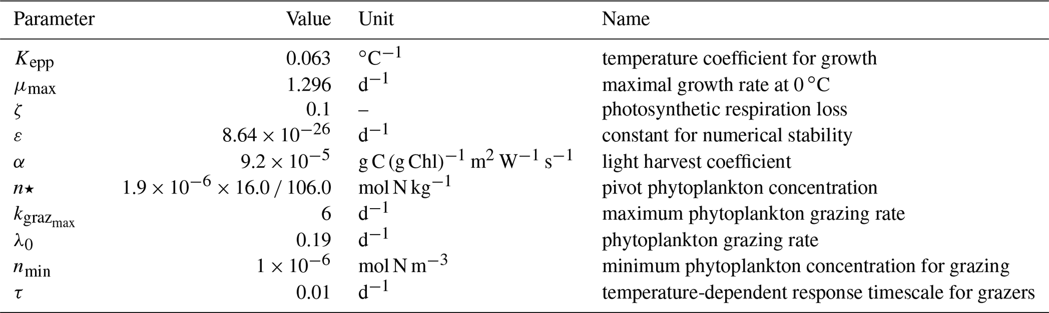
Table A2 Parameter values used in TOPAZv2 to compute the production and grazing of small phytoplankton.

Table A3 Parameter values used in TOPAZv2 to compute the production and grazing of large phytoplankton.

A1.1 Phytoplankton growth

In TOPAZv2, the nitrogen-specific growth rate is defined for all phytoplankton types as follows:

$$\begin{array}{}\text{(A3)}& {\mathit{\mu }}_i={\displaystyle \frac{{\mathit{\mu }}_{max}{N}_{{\lim }_i}{T}_{\mathrm{f}}+\mathit{\epsilon }}{\mathrm{1}+\mathit{\zeta }}}{L}_{{\lim }_i}\approx {\mathit{\mu }}_{max}{N}_{{\lim }_i}{L}_{{\lim }_i}{T}_{\mathrm{f}},\end{array}$$

where N_lim is the nutrient limitation, L_lim is the light limitation, and T_f is an Eppley function of the temperature.

A1.2 Nutrient limitation

N_lim is computed using Liebig’s law of the minimum, where N_Fe, $N_{\mathrm{Si}(\mathrm{OH}{)}_{\mathrm{4}}}$, $N_{{\mathrm{PO}}_{\mathrm{4}}}$, $N_{{\mathrm{NH}}_{\mathrm{4}}}$, and $N_{{\mathrm{NO}}_{\mathrm{3}}}$ correspond to the nutrient limitation specific to iron, silicon, phosphate, ammonia, and nitrate.

$$N_{{\lim }_i}=min\left(N_{{\mathrm{Fe}}_i},N_{{\mathrm{Si}\left(\mathrm{OH}\right)}_{{\mathrm{4}}_i}},N_{{\mathrm{PO}}_{{\mathrm{4}}_i}},N_{{\mathrm{NH}}_{{\mathrm{4}}_i}}+N_{{\mathrm{NO}}_{{\mathrm{3}}_i}}\right)$$

Nutrient limitation is represented according to Michaelis–Menten kinetics, where K_Fe, $K_{{\mathrm{Si}\left(\mathrm{OH}\right)}_{\mathrm{4}}}$, $K_{{\mathrm{PO}}_{\mathrm{4}}}$, $K_{{\mathrm{NH}}_{\mathrm{4}}}$, and $K_{{\mathrm{NO}}_{\mathrm{3}}}$ are the half-saturation constants of each nutrient.

$$\begin{array}{}\text{(A4)}& {\displaystyle }{N}_{{\mathrm{Fe}}_i}={\displaystyle \frac{\mathrm{Fe}}{\mathrm{Fe}+K_{{\mathrm{Fe}}_i}}}\text{(A5)}& {\displaystyle }{N}_{{\mathrm{PO}}_{{\mathrm{4}}_i}}={\displaystyle \frac{{\mathrm{PO}}_{\mathrm{4}}}{{\mathrm{PO}}_{\mathrm{4}}+K_{{\mathrm{PO}}_{{\mathrm{4}}_i}}}}\text{(A6)}& {\displaystyle }{N}_{{\mathrm{Si}\left(\mathrm{OH}\right)}_{{\mathrm{4}}_i}}={\displaystyle \frac{{\mathrm{Si}\left(\mathrm{OH}\right)}_{\mathrm{4}}}{{\mathrm{Si}\left(\mathrm{OH}\right)}_{\mathrm{4}}+K_{{\mathrm{Si}\left(\mathrm{OH}\right)}_{{\mathrm{4}}_i}}}}\text{(A7)}& {\displaystyle }{N}_{{\mathrm{NH}}_{{\mathrm{4}}_i}}={\displaystyle \frac{{\mathrm{NH}}_{\mathrm{4}}}{{\mathrm{NH}}_{\mathrm{4}}+K_{{\mathrm{NH}}_{{\mathrm{4}}_i}}}}\end{array}$$

Nitrate limitation with ammonia inhibition is represented after Frost and Franzen (1992).

$$\begin{array}{}\text{(A8)}& N_{{\mathrm{NO}}_{{\mathrm{3}}_i}}={\displaystyle \frac{{\mathrm{NO}}_{\mathrm{3}}}{{\mathrm{NO}}_{\mathrm{3}}+K_{{\mathrm{NO}}_{{\mathrm{3}}_i}}}}\cdot \left(\mathrm{1}+{\displaystyle \frac{{\mathrm{NH}}_{\mathrm{4}}}{K_{{\mathrm{NH}}_{{\mathrm{4}}_i}}}}\right)\end{array}$$

A1.3 Light limitation

Light limitation is calculated as

$$\begin{array}{}\text{(A9)}& L_{{\lim }_i}=\mathrm{1}-e^{-\frac{{\mathit{\alpha }}_i{\mathit{\theta }}_i\mathrm{Irr}}{N_{{\lim }_i}{T}_{\mathrm{f}}{\mathit{\mu }}_{max}+\mathit{\epsilon }}},\end{array}$$

where α is the light harvest coefficient, θ is the chlorophyll-to-carbon ratio, and Irr corresponds to the mean light level (W m⁻²) of a depth layer. μ_max is the maximal growth rate and ε a constant for numerical stability. More details on how to compute θ, N_Fe, $N_{{\mathrm{PO}}_{\mathrm{4}}}$, and the limitation terms specific to iron and phosphate when Fe : N or P : N varies in phytoplankton are given in Dunne et al. (2013).

A1.4 Temperature function

The temperature function is given as

$$\begin{array}{}\text{(A10)}& T_{\mathrm{f}}=e^{K_{\mathrm{epp}}T},\end{array}$$

where T is the temperature and K_epp is the constant temperature coefficient for growth.

A1.5 Phytoplankton grazing

In TOPAZ, phytoplankton decays through grazing only. Grazing is computed separately for small and large phytoplankton.

$$\begin{array}{}\text{(A11)}& {\displaystyle }{G}_{\mathrm{small}}=min\left(k_{{\mathrm{graz}}_{max}},{\mathit{\lambda }}_{\mathrm{0}}{T}_{\mathrm{f}}{\displaystyle \frac{n_{\mathrm{small}}}{n\star }}\right){\displaystyle \frac{n_{\mathrm{small}}^{\mathrm{2}}}{n_{\mathrm{small}}+n_{min}}},\text{(A12)}& {\displaystyle }\begin{array}{rl}{G}_{\mathrm{large}}=& min\left(k_{{\mathrm{graz}}_{max}},{\mathit{\lambda }}_{\mathrm{0}}{T}_{\mathrm{f}}{\left({\displaystyle \frac{n^{{\mathrm{graz}}_{\mathrm{large}}}}{n\star }}\right)}^{\mathrm{1}/\mathrm{3}}\right.\\ & \left.{\displaystyle \frac{n^{{\mathrm{graz}}_{\mathrm{large}}}}{n_{\mathrm{large}}+n_{min}}}\right)n_{\mathrm{large}},\end{array}\end{array}$$

where $k_{{\mathrm{graz}}_{max}}$ is the maximum grazing rate, λ₀ is another grazing rate, and n⋆ is the pivot phytoplankton concentration for grazing-based variations in ecosystem structure. $n^{{\mathrm{graz}}_{\mathrm{large}}}$ is an implicit phytoplankton concentration after incorporation of a temperature-dependent time lag:

$$\begin{array}{}\text{(A13)}& n^{{\mathrm{graz}}_{\mathrm{large}}}={\left(n^{{\mathrm{graz}}_{\mathrm{large}}}\right)}_{\mathrm{old}}\cdot e^{\frac{n_{\mathrm{large}}-{\left(n^{{\mathrm{graz}}_{\mathrm{large}}}\right)}_{\mathrm{old}}}{n_{\mathrm{large}}+{\left(n^{{\mathrm{graz}}_{\mathrm{large}}}\right)}_{\mathrm{old}}}\cdot \mathrm{2}\cdot min\left(\mathrm{1},T_{\mathrm{f}}\frac{\mathrm{\Delta }t}{\mathit{\tau }}\right)},\end{array}$$

where $(n^{{\mathrm{graz}}_{\mathrm{large}}}{)}_{\mathrm{old}}$ corresponds to $n^{{\mathrm{graz}}_{\mathrm{large}}}$ of the previous time step Δt and τ is the temperature-dependent response timescale for grazers, which is set to a very small number to simulate instantaneous response. More explanations are given in Dunne et al. (2013). Parameter values used in TOPAZv2 to compute phytoplankton production and grazing are provided in Tables A1, A2, and A3.

A2 CESM2: MARBL

The Marine Biogeochemistry Library (MARBL) is the biogeochemical component of CESM2. It is a prognostic ocean biogeochemistry model that simulates marine-ecosystem dynamics and the coupled cycles of carbon, nitrogen, phosphorus, iron, silicon, and oxygen (M. C. Long et al., 2021). Three phytoplankton types are represented: small phytoplankton, diatoms, and diazotrophs. The concentration P_i of each phytoplankton type i is a prognostic variable.

$$\begin{array}{}\text{(A14)}& {\partial }_t{P}_i={\mathrm{NPP}}_i-{\mathrm{Loss}}_i+{\mathrm{Circ}}_i,\end{array}$$

where Loss corresponds to phytoplankton decay and Circ corresponds to the physical advection and mixing of phytoplankton by ocean circulation. The NPP of each phytoplankton type is the product of its growth rate μ and its biomass n:

$$\begin{array}{}\text{(A15)}& {\mathrm{NPP}}_i={\mathit{\mu }}_i{P}_i.\end{array}$$

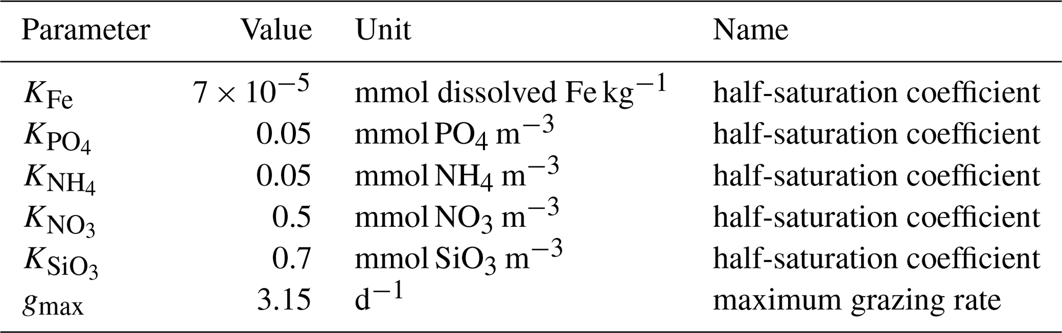
Table A4 Parameter values used in MARBL to compute the production and loss of small and large phytoplankton.

Table A5 Parameter values used in MARBL to compute the production and loss of small phytoplankton.

Table A6 Parameter values used in MARBL to compute the production and loss of large phytoplankton.

A2.1 Phytoplankton growth

In MARBL, the carbon-specific growth rate of phytoplankton is defined as

$$\begin{array}{}\text{(A16)}& {\mathit{\mu }}_i={\mathit{\mu }}_{\mathrm{ref}}{N}_{{\lim }_i}{L}_{{\lim }_i}{T}_{\mathrm{f}},\end{array}$$

where μ_ref is a constant accounting for the maximum growth rate at the reference temperature of 30 ^∘C. N_lim is the nutrient limitation; L_lim is the light limitation; T_f is the temperature function.

A2.2 Nutrient limitation

N_lim is computed using Liebig's law of the minimum, where N_Fe, $N_{{\mathrm{SiO}}_{\mathrm{3}}}$, N_P, $N_{{\mathrm{NH}}_{\mathrm{4}}}$, and $N_{{\mathrm{NO}}_{\mathrm{3}}}$ correspond to the nutrient limitation specific to iron, silicon, phosphate, ammonia, and nitrate.

$$\begin{array}{}\text{(A17)}& N_{{\lim }_i}=min\left(N_{{\mathrm{Fe}}_i},N_{{\mathrm{SiO}}_{{\mathrm{3}}_i}},N_{{\mathrm{P}}_i},N_{{\mathrm{NH}}_{{\mathrm{4}}_i}}+N_{{\mathrm{NO}}_{{\mathrm{3}}_i}}\right)\end{array}$$

$$\begin{array}{}\text{(A18)}& N_{{\mathrm{Fe}}_i}={\displaystyle \frac{\mathrm{Fe}}{\mathrm{Fe}+K_{{\mathrm{Fe}}_i}}}\end{array}$$

$$\begin{array}{}\text{(A19)}& N_{{\mathrm{SiO}}_{{\mathrm{3}}_i}}={\displaystyle \frac{{\mathrm{SiO}}_{\mathrm{3}}}{{\mathrm{SiO}}_{\mathrm{3}}+K_{{\mathrm{SiO}}_{{\mathrm{3}}_i}}}}\end{array}$$

Phytoplankton can alternatively assimilate nitrate and ammonium following O'Neill et al. (1989), such that

$$\begin{array}{}\text{(A20)}& N_{{\mathrm{NH}}_{{\mathrm{4}}_i}}={\displaystyle \frac{\frac{{\mathrm{NH}}_{\mathrm{4}}}{K_{{\mathrm{NH}}_{{\mathrm{4}}_i}}}}{\mathrm{1}+\frac{{\mathrm{NO}}_{\mathrm{3}}}{K_{{\mathrm{NO}}_{{\mathrm{3}}_i}}}+\frac{{\mathrm{NH}}_{\mathrm{4}}}{K_{{\mathrm{NH}}_{{\mathrm{4}}_i}}}}},\end{array}$$

$$\begin{array}{}\text{(A21)}& N_{{\mathrm{NO}}_{{\mathrm{3}}_i}}={\displaystyle \frac{\frac{{\mathrm{NO}}_{\mathrm{3}}}{K_{{\mathrm{NO}}_{{\mathrm{3}}_i}}}}{\mathrm{1}+\frac{{\mathrm{NO}}_{\mathrm{3}}}{K_{{\mathrm{NO}}_{{\mathrm{3}}_i}}}+\frac{{\mathrm{NH}}_{\mathrm{4}}}{K_{{\mathrm{NH}}_{{\mathrm{4}}_i}}}}}.\end{array}$$

Phytoplankton is able to assimilate phosphorus in the form of phosphate (PO₄) and semi-labile dissolved organic phosphate (DOP); a similar approach is used to compute N_P.

A2.3 Light limitation

The light limitation is given as

$$\begin{array}{}\text{(A22)}& L_{{\lim }_i}=\mathrm{1}-e^{-\frac{{\mathit{\alpha }}_i{\mathit{\theta }}_i\mathrm{Irr}}{N_{{\lim }_i}{T}_{\mathrm{f}}{\mathit{\mu }}_{\mathrm{ref}}}},\end{array}$$

where α is the light harvest coefficient; θ is the chlorophyll-to-carbon ratio; and Irr corresponds to the photosynthetically available radiation, defined as 45 % of incoming shortwave radiation (W m⁻²). In the high latitudes, CESM2 simulates a subgrid-scale sea-ice thickness distribution and computes shortwave penetration independently in each sub-column. MARBL then takes an area-weighted average across sub-columns to compute the grid cell mean light level. For more details on how to compute θ and N_P, see M. C. Long et al. (2021).

A2.4 Temperature function

The temperature function is given as

$$\begin{array}{}\text{(A23)}& T_{\mathrm{f}}={\mathrm{1.7}}^{\frac{T-\mathrm{30}{}^{\circ }\mathrm{C}}{\mathrm{10}{}^{\circ }\mathrm{C}}},\end{array}$$

where T is the temperature.

A2.5 Phytoplankton loss

In MARBL, phytoplankton decays through grazing G, mortality M, and aggregation A, which refers to the process by which dying phytoplankton form aggregates that sink through the water column. The three loss terms depend on P^′, the phytoplankton concentration in excess of a temperature- and depth-dependent threshold (M. C. Long et al., 2021).

$$\begin{array}{}\text{(A24)}& {\displaystyle }{P}_i^{\prime }=max\left(P_i-P_{{\mathrm{threshold}}_i},\mathrm{0}\right)\text{(A25)}& {\displaystyle }{\mathrm{Loss}}_i=G(P_i^{\prime }{)}_i+M(P_i^{\prime })+A_{i_i}(P_i^{\prime })\end{array}$$

Grazing by zooplankton is given as

$$\begin{array}{}\text{(A26)}& G_i\left(P_i^{\prime }\right)=g_{{max}_i}{T}_{\mathrm{f}}{\displaystyle \frac{P_i^{\prime }}{K^{\mathrm{P}}+P_i^{\prime }}}z,\end{array}$$

where g_max is the maximum grazing rate, K^P is the half-saturation constant for phytoplankton grazing, and z is the zooplankton biomass.

Mortality is given as

$$\begin{array}{}\text{(A27)}& M\left(P_i^{\prime }\right)=m{T}_{\mathrm{f}}{P}_i^{\prime },\end{array}$$

where m is the linear mortality rate.

Finally, aggregation is parameterized as

$$\begin{array}{}\text{(A28)}& A_i\left(P_i^{\prime }\right)=a_i\times (P_i^{\prime }{)}^{\mathrm{1.75}},\end{array}$$

where a is the aggregation rate (see M. C. Long et al., 2021, for more details). Parameter values used in MARBL to compute phytoplankton production and loss are provided in Tables A4, A5, and A6.

Appendix B: Additional figures

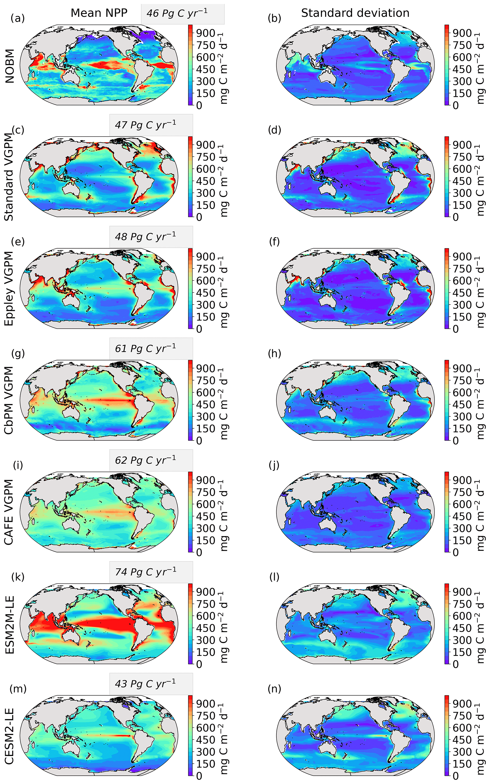
Figure B1 Climatological mean and standard deviation of the observation-based NPP estimates (mg C m⁻² d⁻¹) calculated from NOBM (a, b), Standard VGPM (c, d), Eppley-VGPM (e, f), CbPM (g, h), and CAFE (i, j) and simulated by ESM2M-LE (k, l) and CESM2-LE (m, n) over 1998–2018. Gray boxes indicate the globally integrated mean NPP (Pg C yr⁻¹). We use 5 d mean NPP output for all products except for the VGPM-based products (c–j).

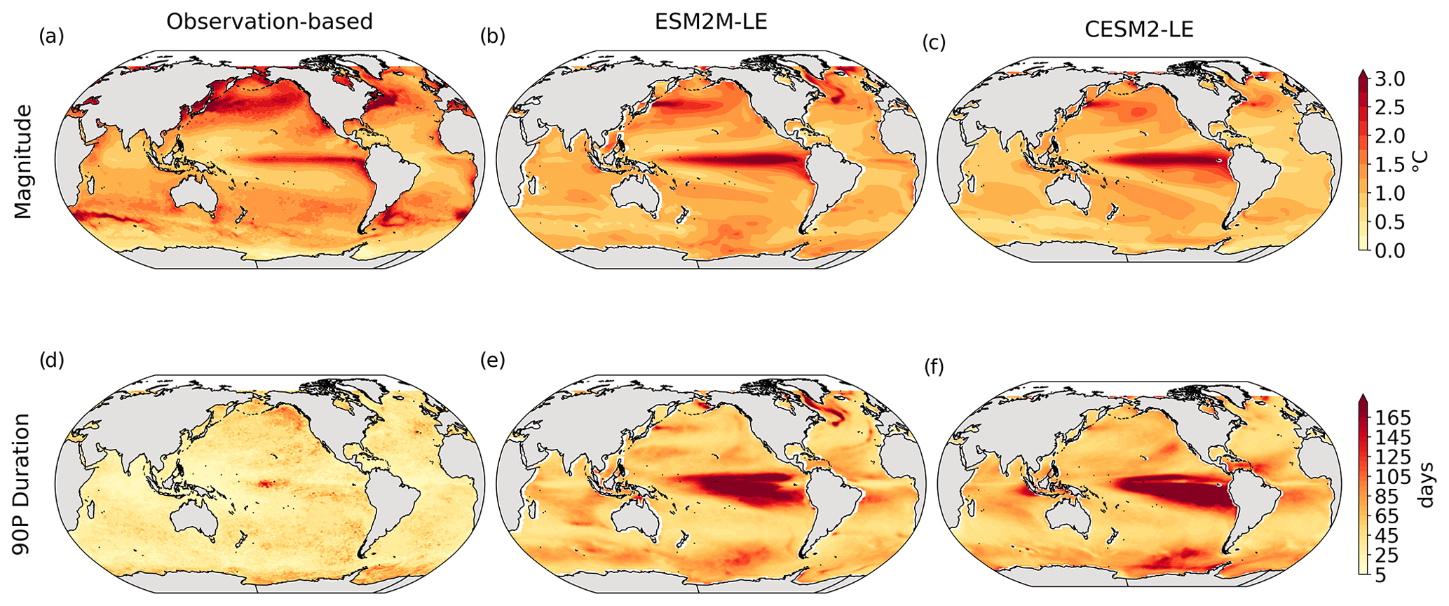
Figure B2 Simulated mean magnitude and duration of MHWs over 1998–2018. Mean SST anomaly relative to the seasonal cycle (^∘C) during MHWs in (a) the observation-based estimate, (b) ESM2M-LE, and (c) CESM2-LE. Simulated 90th percentile of the MHW durations (days) in (d) the observation-based estimate, (e) ESM2M-LE, and (f) CESM2-LE. The global mean magnitude equals 1.3, 1.2, and 1.2 ^∘C, while the global mean 90th percentile of the duration equals 36, 69, and 75 d in the observations, ESM2M-LE, and CESM2-LE, respectively.

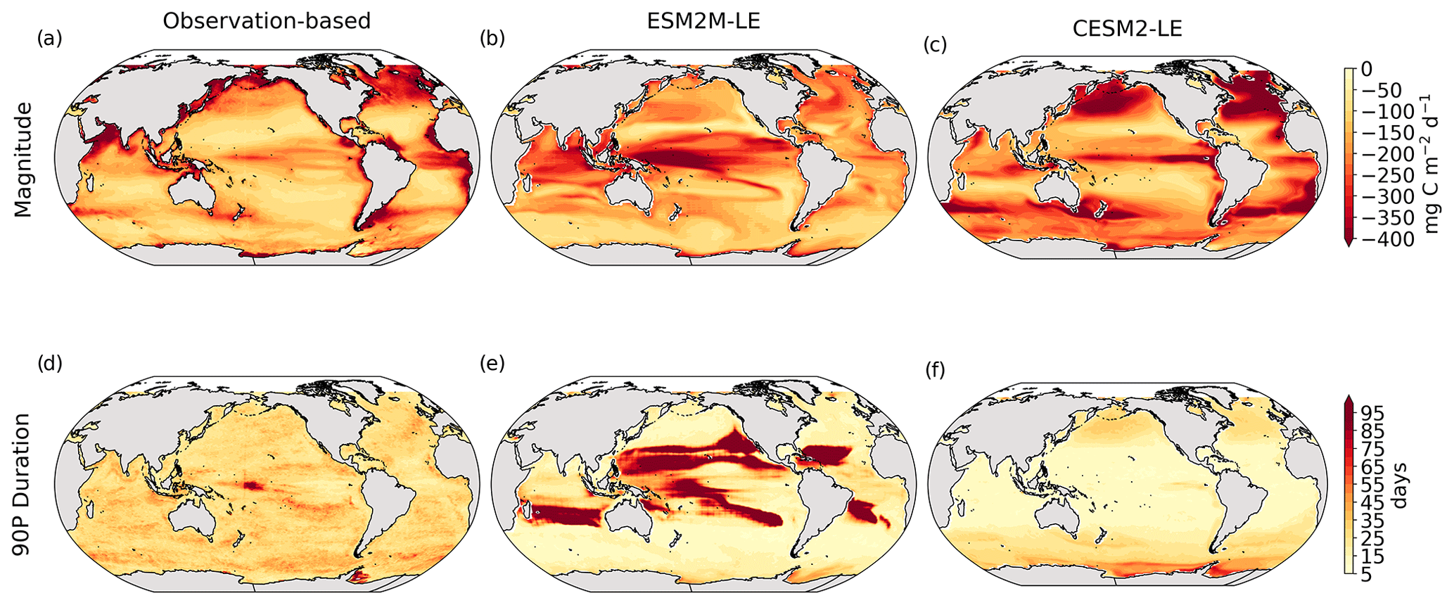
Figure B3 Simulated mean magnitude and duration of NPPX events over 1998–2018. Mean NPP anomaly relative to the seasonal cycle (mg C m⁻² d⁻¹) during NPPX events in (a) observation-based estimates, (b) ESM2M-LE, and (c) CESM2-LE. The 90th percentile of the NPPX events duration (days) in (d) observation-based estimates, (e) ESM2M-LE, and (f) CESM2-LE. The global mean magnitude equals −209, −182 and −223 mg C m⁻² d⁻¹, while the global mean 90th percentile of the duration equals 29, 34, and 18 d in the observations, ESM2M-LE, and CESM2-LE, respectively.

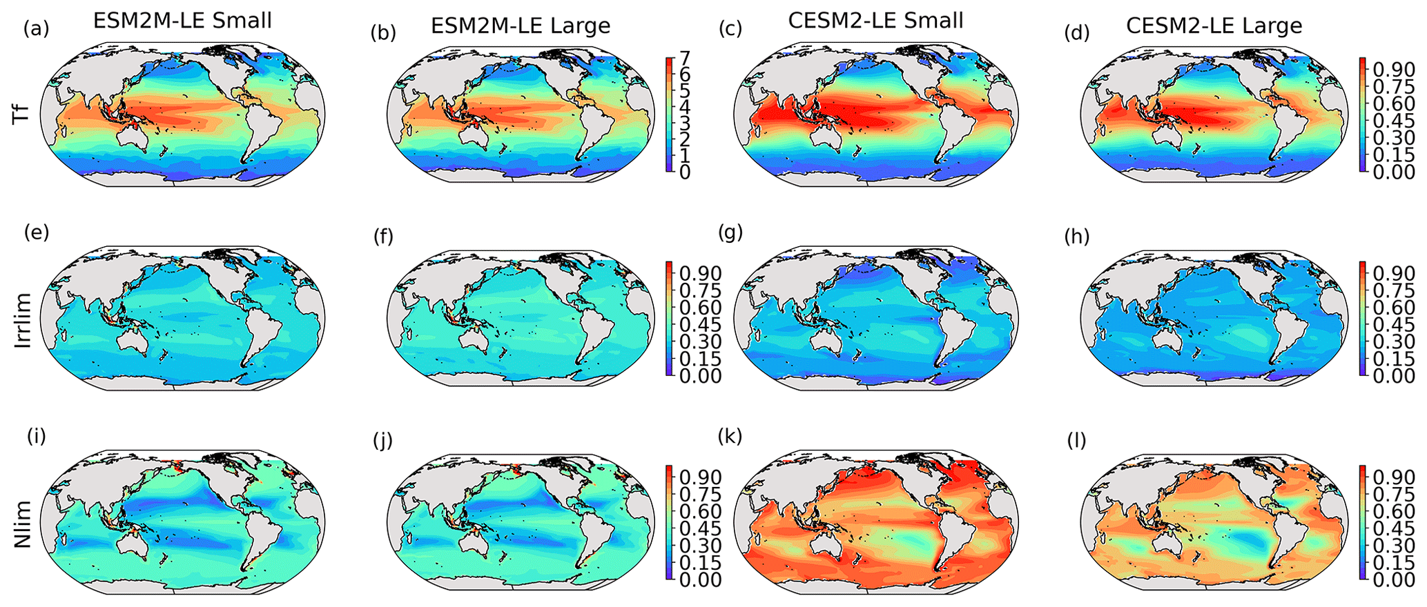
Figure B4 Simulated mean states of the temperature (a–d, T_f), light (e–h, Irr_lim), and nutrient (i–l, N_lim) limitations on the small- and large-phytoplankton growth rates in ESM2M-LE and CESM2-LE over 1998–2018.

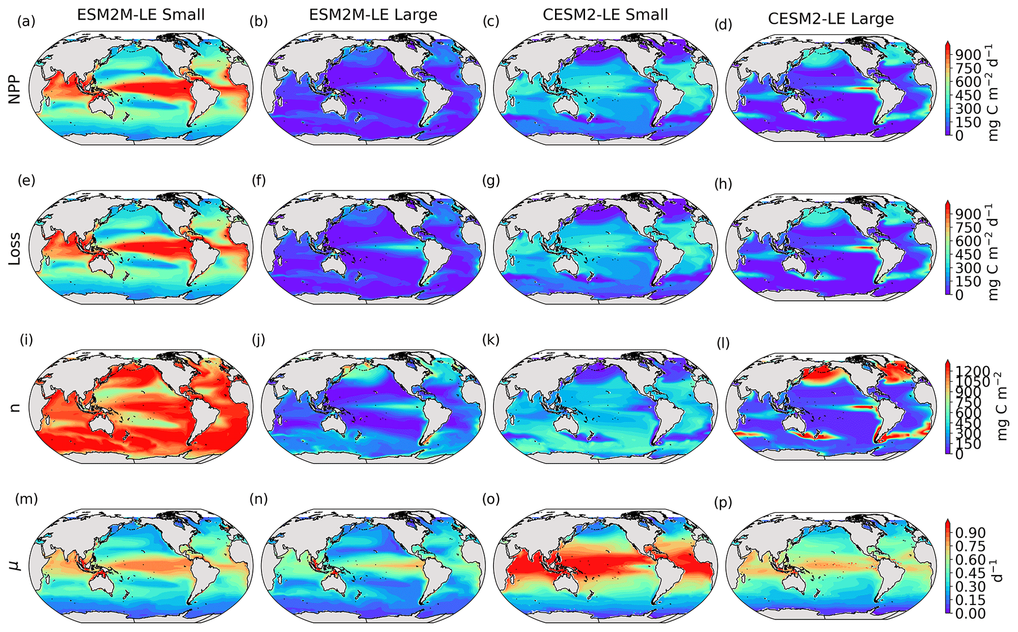
Figure B5 Simulated mean states of small- and large-phytoplankton NPP (a–d, mg C m⁻² d⁻¹), loss (e–h, mg C m⁻² d⁻¹), biomass (i–l, mg C m⁻²), and growth rates (m–p, d⁻¹) in ESM2M-LE and CESM2-LE over 1998–2018.

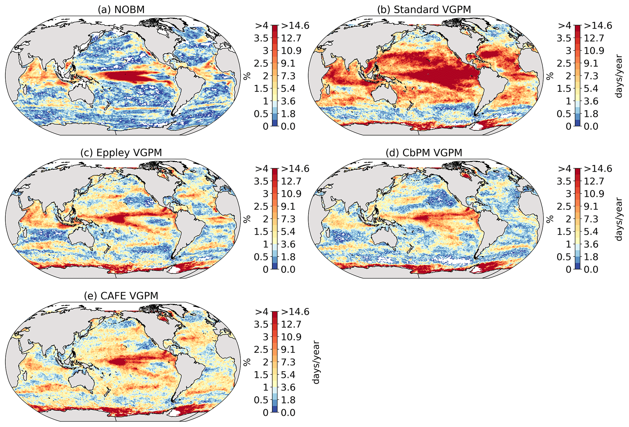
Figure B6 Likelihood (%) of compound MHW–NPPX events estimated using the observation-based NPP product of (a) NOBM, (b) Standard VGPM, (c) Eppley-VGPM, (d) CbPM-VGPM, and (e) CAFE-VGPM.

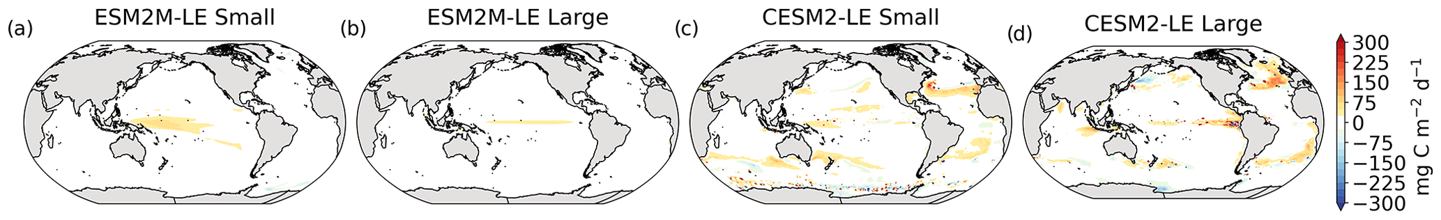
Figure B7 Difference between the NPP anomaly dNPP during compound MHW–NPPX events and its decomposition into a contribution of the growth rate anomaly ndμ and of the biomass anomaly μdn (mg C m⁻² d⁻¹) during compound MHW–NPPX events for small and large phytoplankton in ESM2M-LE (a, b) and in CESM2-LE (c, d).

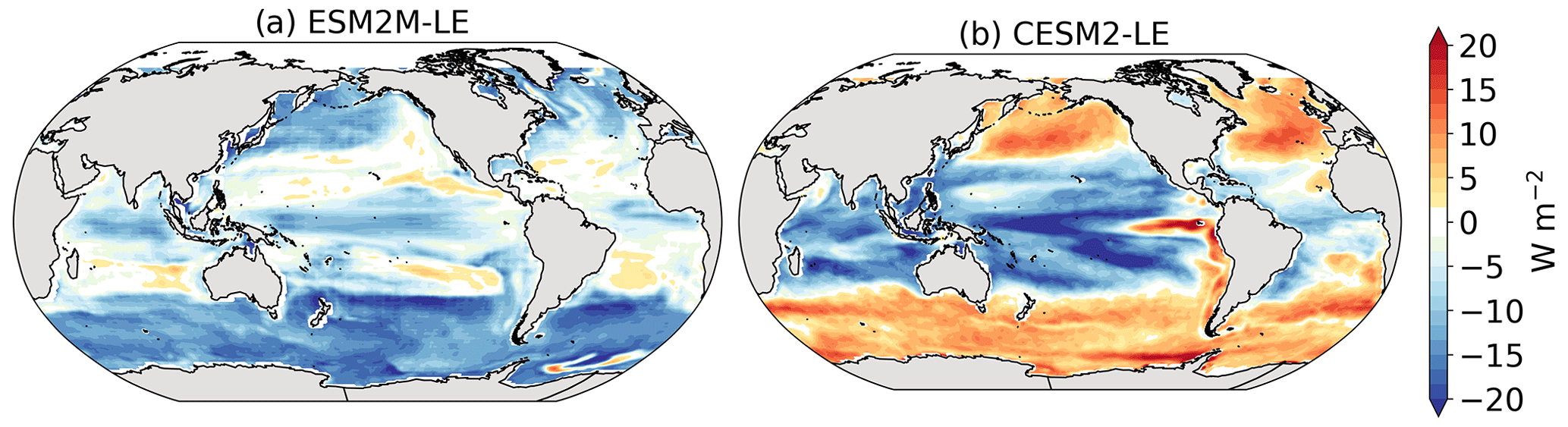
Figure B8 Surface photosynthesis available radiation anomaly (W m⁻²) during MHW–NPPX events relative to the seasonal cycle in ESM2M-LE (a) and in CESM2-LE (b).

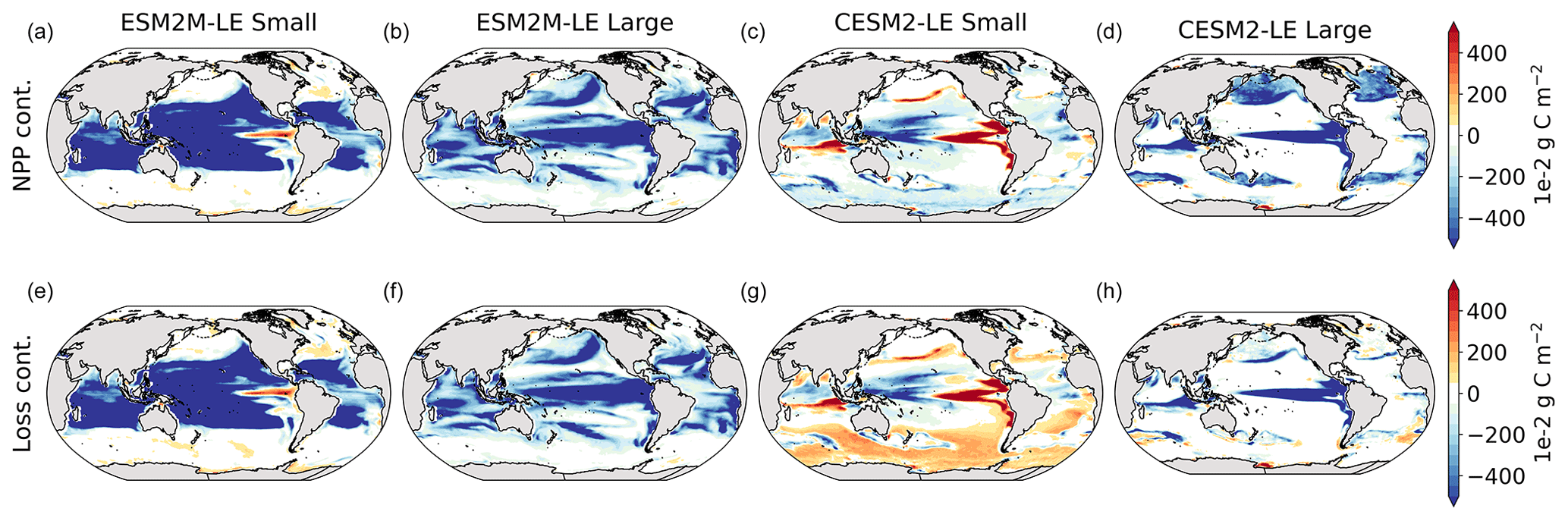
Figure B9 Contributions (1 × 10⁻² g C m⁻² d⁻¹) of small- and large-phytoplankton NPP and Loss to the buildup of the maximum biomass anomaly (mg C m⁻² d⁻¹) in ESM2M-LE (a, b, e, f) and in CESM2-LE (c, d, g, h).

Figure B10 Difference between the integrated biomass change Δn (Fig. 5e–h) and the NPP−Loss contribution to Δn (Fig. 5i–l). This residual term includes the circulation contribution to Δn and all errors inherent to the decomposition in Eq. (8).