Assessing the sensitivity of multi-frequency passive microwave vegetation optical depth to vegetation properties

Vegetation attenuates the microwave emission from the land surface. The strength of this attenuation is quantified in models in terms of the parameter vegetation optical depth (VOD) and is influenced by the vegetation mass, structure, water content, and observation wavelength. Earth observation satellite sensors operating in the microwave frequencies are used for global VOD retrievals, enabling the monitoring of vegetation at large scales. VOD has been used to determine above-ground biomass, monitor phenology, or estimate vegetation water status. VOD can be also used for constraining land surface models or modelling wildfires at large scales. Several VOD products exist, differing by frequency/wavelength, sensor, and retrieval algorithm. Numerous studies present correlations or empirical functions between different VOD datasets and vegetation variables such as the normalized difference vegetation index, leaf area index, gross primary production, biomass, vegetation height, or vegetation water content. However, an assessment of the joint impact of land cover, vegetation biomass, leaf area, and moisture status on the VOD signal is challenging and has not yet been done.

This study aims to interpret the VOD signal as a multi-variate function of several descriptive vegetation variables. The results will help to select VOD at the most suitable wavelength for specific applications and can guide the development of appropriate observation operators to integrate VOD with large-scale land surface models. Here we use VOD from the Land Parameter Retrieval Model (LPRM) in the Ku, X, and C bands from the harmonized Vegetation Optical Depth Climate Archive (VODCA) dataset and L-band VOD derived from Soil Moisture and Ocean Salinity (SMOS) and Soil Moisture Active Passive (SMAP) sensors. The leaf area index, live-fuel moisture content, above-ground biomass, and land cover are able to explain up to 93 % and 95 % of the variance (Nash–Sutcliffe model efficiency coefficient) in 8-daily and monthly VOD within a multi-variable random forest regression. Thereby, the regression reproduces spatial patterns of L-band VOD and spatial and temporal patterns of Ku-, X-, and C-band VOD. Analyses of accumulated local effects demonstrate that Ku-, X-, and C-band VOD are mostly sensitive to the leaf area index, and L-band VOD is most sensitive to above-ground biomass. However, for all VODs the global relationships with vegetation properties are non-monotonic and complex and differ with land cover type. This indicates that the use of simple global regressions to estimate single vegetation properties (e.g. above-ground biomass) from VOD is over-simplistic.

1 Introduction

Vegetation optical depth (VOD) describes the attenuation of microwave radiation in the vegetation layer. Quantifying this attenuation effect is important for an accurate retrieval of surface soil moisture from passive microwave satellite observations (Wang, 1985; Njoku and Entekhabi, 1996). In the radiative transfer equation for microwave emissions, the opacity of the vegetation layer (i.e. the VOD) is also commonly referred to as τ (Jackson et al., 1982). VOD can be retrieved e.g. from the passive microwave radiative transfer equation using measurements of passive microwaves (Jackson and Schmugge, 1991; Owe et al., 2008; Sawada et al., 2016). However, VOD is a parameter in these microwave radiative transfer models for vegetation, and hence it is not directly measurable and verifiable with in situ measurements. Therefore, different authors have correlated VOD with different vegetation properties to understand the sensitivity of VOD to vegetation properties (Jones et al., 2011; Rodríguez-Fernández et al., 2018; Konings et al., 2019a). Generally, the opacity of passive microwaves in the vegetation layer increases with increasing vegetation water content, but this relationship varies with vegetation structure including leaf and woody components and wavelength (Jackson and Schmugge, 1991; Wigneron et al., 1993; Njoku and Entekhabi, 1996). Based on radiometer measurements over various crops and a wide range of wavelengths (0.8–30 cm), Jackson and Schmugge (1991) report a clear linear relationship of VOD to vegetation water content (VWC):

$$\begin{array}{}\text{(1)}& \mathrm{VOD}=b\cdot \mathrm{VWC},\end{array}$$

where the parameter b depends on vegetation type and wavelength. The authors find that b exponentially decreases with increasing wavelength, which implies that vegetation opacity (the VOD) is smaller for longer wavelengths (i.e. L band) than for shorter wavelengths (i.e. Ku, X, and C bands). The parameter b is usually kept constant for one vegetation type and wavelength, which might be insufficient due to its possible dependency on polarization. In addition, neglecting surface soil roughness can lead to an underestimation of VOD, especially when the vegetation does not completely cover the ground (Togliatti et al., 2022).

The vegetation water content can also be expressed as a product of above-ground biomass (AGB) and a parameter of relative water content, often referred to as live-fuel moisture content (LFMC) (Konings et al., 2019b),

$$\begin{array}{}\text{(2)}& \mathrm{VOD}=b\cdot \mathrm{AGB}\cdot \mathrm{LFMC},\end{array}$$

whereby LFMC is defined as the ratio of water mass in the vegetation to the dry mass of the vegetation usually expressed in percentage (Konings et al., 2019b),

$$\begin{array}{}\text{(3)}& \mathrm{LFMC}={\displaystyle \frac{M_{\mathrm{f}}-M_{\mathrm{d}}}{M_{\mathrm{d}}}}\cdot \mathrm{100},\end{array}$$

with M_f as the fresh mass of vegetation and M_d as the dry mass of vegetation.

Based on these relationships, many studies use VOD to estimate AGB or other vegetation properties. For example, Liu et al. (2015) use Ku-band VOD to estimate long-term changes in global AGB, finding a gain of above-ground biomass carbon considering forest and non-forest vegetation for 1993–2012. Rodríguez-Fernández et al. (2018) correlate spatial patterns in AGB and yearly averaged values of L-band VOD from the Soil Moisture and Ocean Salinity (SMOS) mission with the INRA-CESBIO (Institut National de la Recherche Agronomique Centre d'Etudes Spatiales de la Biosphère) algorithm (SMOS-IC) for Africa with correlation coefficients up to 0.85. They find linear relationships between VOD and AGB within single land cover classes, but the relationship across land cover classes is shown to be non-linear, with a weaker non-linearity for L-band VOD compared to Ku-/X-/C-band VOD. Chaparro et al. (2018) use the L band from the Soil Moisture Active Passive mission (SMOS) derived with the multi-temporal dual-channel algorithm (MT-DCA) to determine crop biomass of the north-central USA. Both Rodríguez-Fernández et al. (2018) and Chaparro et al. (2018) find better results for pixels with higher homogeneity in land cover types or even plant types, implying that relationships between VOD and vegetation properties change with land cover and plant types. X. Li et al. (2021) find a high correlation of L-band VOD and AGB leading to the conclusion that long-wave VOD is more sensitive to woody parts of the vegetation than short-wave VOD. However, Konings et al. (2021) show that the relation between L-band VOD and AGB dominates in space but that short-term temporal dynamics in VOD are dominated by VWC. As a proxy for vegetation water status, VOD can be related to LFMC or VWC or both (Fan et al., 2018; Konings et al., 2019b; Frappart et al., 2020) and can be used to estimate leaf water potential (Konings and Gentine, 2017; Momen et al., 2017; Zhang et al., 2019).

Furthermore, VOD is frequently compared with other vegetation properties such as canopy greenness, the leaf area index (LAI), or plant productivity. For example, VOD shows similar temporal patterns to the normalized difference vegetation index (NDVI) and LAI (Liu et al., 2011; Momen et al., 2017; Bousquet et al., 2021). In spatial comparisons, the vegetation indices and variables tend to saturate over densely vegetated areas. This saturation is less distinct for VOD (Rodríguez-Fernández et al., 2018) due to the ability of microwaves to penetrate deeper into the vegetation layer. Therefore, VOD provides complementary information to the usually visible–infrared-based metrics (Jones et al., 2011). For example, metrics sensitive to biomass or water content shifts can be derived from VOD (Jones et al., 2011, 2014). VOD can also be used for assessing land surface phenology (Jones et al., 2011). VOD and temporal changes in VOD are also correlated with gross primary production (GPP) (Teubner et al., 2018), which allows VOD to be used as a predictor of GPP (Teubner et al., 2019, 2021; Wild et al., 2022).

Recently, several new VOD datasets have become available for the X band from the Advanced Microwave Scanning Radiometer – Earth Observing System sensor (AMSR-E) and Advanced Microwave Scanning Radiometer 2 (AMSR2) sensors (Du et al., 2017; Wang et al., 2021) and for the L band from the SMOS (van der Schalie et al., 2016; Fernandez-Moran et al., 2017; Al Bitar et al., 2017; Wigneron et al., 2018, 2021) and Soil Moisture Active Passive sensors (SMAP; Konings et al., 2017). VOD was also retrieved jointly from several sensors (van der Schalie et al., 2017), and harmonized long-term multi-sensor datasets have been produced (e.g. Vegetation Optical Depth Climate Archive, VODCA, Moesinger et al., 2020). A recent comparison study by Li et al. (2021) of different X-, C-, and L-band VOD datasets and Moderate Resolution Imaging Spectroradiometer-derived (MODIS) vegetation indices like NDVI and the enhanced vegetation index (EVI) as well as tree height and AGB showed that X-band VOD is more suitable to detect temporal variations of the green vegetation parts, especially for less densely vegetated areas, than C- and L-band VOD. Additionally, Li et al. (2021) as well as Moesinger et al. (2022) found time lags between VOD and vegetation indices and climate variables, which are not yet fully understood. This shows the need to include further ecological parameters or vegetation variables which could account for a delayed response of VOD to temporal changes in the vegetation indices. Approaches with the ability to consider VOD variations caused by vegetation water content have been developed, which are more complex than simple regression functions (e.g. Momen et al., 2017). Momen et al. (2017) were able to estimate VOD by using two predictors, LAI and leaf water potential. Among others, the studies by Momen et al. (2017) and Teubner et al. (2019) show that the water content of the vegetation influences VOD and therefore affects not only the relation between vegetation indices and VOD but also the relation between VOD and AGB.

The increasing availability of VOD data for vegetation studies also increases the possibilities for assimilating or integrating VOD with ecosystem or land surface models (LSMs) (Scholze et al., 2019; Kumar et al., 2020). Therefore, observation operators are needed that link the modelled vegetation properties with the satellite-retrieved VOD. Scholze et al. (2019) use the sum of an empirical AGB function and a linear term for LAI to describe annual SMOS-IC L-band VOD within the carbon cycle data assimilation system (CCDAS) for estimating European carbon fluxes. Kumar et al. (2020) use cumulative distribution function (CDF) matching to convert VODCA X- and C-band VOD and SMAP L-band VOD to LAI, which is then assimilated into the Noah-MP (Multiparameterization) LSM. X- and L-band VOD showed partially complementary improvements in the modelled land surface variables. Both studies by Scholze et al. (2019) and Kumar et al. (2020) find an improvement in the model results by incorporating passive microwave data, demonstrating the benefits of the vegetation information contained in VOD. In another model-data-fusion approach, Liu et al. (2021) use VOD to derive plant hydraulic parameters for a soil–plant system model that accounts for the hydraulic state of the vegetation explicitly. However, as VOD reflects both dynamics in biomass and water content (Jackson and Schmugge, 1991; Konings et al., 2021), relations between VOD and AGB or LAI as observation operators are simplifications and demonstrate the need for a more detailed understanding of the effects of vegetation properties on VOD.

The increasing use of VOD for ecosystem studies (e.g. Dorigo et al., 2021) and land surface modelling poses the question of how different vegetation properties affect VOD in both time and space. Hence, a more detailed investigation of the relative effects of vegetation properties on VOD could improve the understanding of the VOD signal in terms of interpretation of the corresponding vegetation status. Such investigations will also help to identify a suitable VOD dataset for a specific ecological application in addition to the technical aspects of the datasets like the observation resolution depending on wavelength, errors, and artefacts induced by the retrieval algorithm or the observation time depending on overpass times of the satellites.

Furthermore, due to the high temporal resolution and temporal coverage of VOD datasets (partly since 1987), global analyses of vegetation properties and status as well as land cover change can be conducted for enhanced understanding of long-term environmental changes and to improve model predictions.

Here we aim to assess VOD in response to multiple vegetation properties at large (i.e. inter-continental) scales. Specifically, our objectives are to predict VOD from LFMC, LAI, and AGB by using two machine learning regression approaches and to investigate the relationship between VOD and the predictors. This objective goes beyond previous empirical studies that compared VOD with vegetation properties based on bivariate correlations or regressions but not by estimating VOD within a multi-variate framework.

We use random forests (RFs) and generalized additive models (GAMs) to predict VOD from LFMC, LAI, AGB, and land cover. Accumulated local effect (ALE) curves are used to assess the sensitivities of VOD to these properties. While GAM is suitable to capture non-linear and non-monotonic relationships with additive effects of the predictors, a random forest (RF) approach can predict more complex interactions but is less suitable to capture a possible additive behaviour. Therefore, comparing both machine learning algorithms gives insights into the structure of the relationship between VOD and vegetation properties and provides confidence in the findings. Additionally, we inspect how different temporal resolutions (i.e. 8-daily and monthly data) affect the relationships between VOD and vegetation properties for identifying the role of vegetation variables at quasi-weekly and seasonal timescales. The analyses are carried out for five VOD datasets, which differ in wavelength but were derived with the same algorithm (Land Parameter Retrieval Model, LPRM) (van der Schalie et al., 2016, 2017) to exclude differences due to retrieval algorithms.

2 Data and methods

2.1 Datasets

2.1.1 VOD data

An overview of the datasets is given in Table 1 and Fig. 1. All used VOD datasets are derived from passive sensors using the LPRM algorithm (van der Schalie et al., 2016) to reduce the degrees of freedom of this analysis. Thereby, for each wavelength a different parametrization was used with the exception of the retrieval of X- and C-band VOD where an identical implementation of single-scattering albedo was applied. For roughness a constant parametrization is used for the Ku band, but a dynamical parameter is used for the other wavelengths. Hence the parametrization essentially differs for the wavelengths. This can affect the similarity of the datasets but is necessary to allow for valid retrievals in general.

The VODCA dataset (Moesinger et al., 2020) provides harmonized long-term records of short-wave VOD for the Ku, X, and C band (further named Ku-VOD, X-VOD, and C-VOD, respectively), using data from the AMSR-E, AMSR2, Special Sensor Microwave Imager (SSM/I), Tropical Rainfall Measuring Mission (TRMM) Microwave Imager (TMI), and WindSat sensors. Unfortunately, Ku-VOD is only available until 1 August 2017 due to a bias in the AMSR2 Ku-band VOD causing unexpected low values of the VOD retrievals after this date (Moesinger et al., 2020), which is not fixed in version 01.0. Therefore, all datasets are analysed until 31 July 2017.

Two LPRM-derived L-band VOD datasets are used as long-wave VOD, one sensed with SMAP, the other with SMOS (van der Schalie et al., 2016; further named SMAP L-VOD and SMOS L-VOD, respectively). The SMAP satellite was launched in January 2015, and therefore SMAP L-VOD defines the start date of the analysis of all datasets.

All VOD datasets are provided as daily data with a spatial resolution of 0.25^∘ on a global scale. As VOD generally decreases with increasing wavelength, the five VOD datasets have different dynamic ranges. As we are not interested in the absolute value but only the temporal dynamics and spatial patterns, the VOD datasets were globally normalized using a minimum and maximum value to a range of 0 to 1 based on the available global data within the time span 2015–2017 to provide comparability. For normalization we use the scikit-learn function “MinMaxScaler”. The normalized VOD data form the basis of Fig. 1d–h. These maps of temporally averaged VOD data show different patterns and scales even after the normalization process. This illustrates that VOD data derived from different wavelengths and sensors are not related to the same vegetation properties, indicating the need for this study.

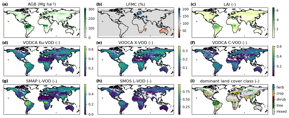
Figure 1 Overview of the datasets used for (a) above-ground biomass (AGB) for 2017 based on the ESA CCI biomass dataset; (b) live-fuel moisture content (LFMC) derived from MODIS, whereby grey indicates areas of non-available data; (c) the leaf area index (LAI) derived from MODIS; (d) Ku-band VOD (Ku-VOD) from VODCA; (e) X-band VOD (X-VOD) from VODCA; (f) C-band VOD (C-VOD) from VODCA; (g) L-band VOD from SMAP (SMAP L-VOD); (h) L-band VOD from SMOS (SMOS L-VOD); and (i) the dominant land cover class for 2016 based on the ESA CCI Land Cover map. LAI, LFMC, and VOD maps are temporal averages over the period January 2015–July 2017, whereby the VOD maps are based on data scaled to 0–1 for the available range within the mentioned time span. Note that LFMC is only available for the western USA, South Africa, Europe, and Australia.

2.1.2 Predictor data

Following the relationship between VOD, LFMC, and AGB as shown in Eq. (2), proxies related to biomass (AGB and LAI), water content (LFMC), and the structure parameter (plant types) are used as predictors for VOD.

As proxies for woody and non-woody biomass, we used a map of AGB and a time series of LAI. The ESA Climate Change Initiative (CCI) AGB map (Santoro and Cartus, 2019) for the year 2017 with a 100 m spatial resolution is used as a predictor of woody biomass. This AGB map describes the oven-dry mass of woody parts of living trees per pixel. Thereby only above-ground mass is considered, i.e. stem and bark as well as twigs and branches but not stumps and roots.

LAI is used as a proxy for canopy biomass. Specifically, we use the MOD15A2H Version 6 dataset from MODIS, which is available at a 500 m spatial and 8-daily temporal resolution on a global scale (Myneni et al., 2015). We excluded LAI retrievals under (partial) cloud cover, snow, or a high solar zenith angle.

For LFMC, we used a product derived from MODIS MCD43A2 Collection 6 reflectance data for the western USA, South Africa, and Australia (Fig. 1b) at a 500 m spatial and 4-daily temporal resolution using the approach described in Yebra et al. (2018). The extent of the western USA region is determined for the purpose of covering California, wherefor the MODIS tiles h08v04, h08v05, and h09v04 were necessary and the tile h09v05 was not considered in favour of computational resources. Yebra et al. (2018) use three radiative transfer models (RTMs) for the simulation of spectra corresponding to different LFMC values. More specifically, they use PROSPECT 1 (Platform for Resource Observation and in-Situ Prospecting for Exploration, Commercial exploitation and Transportation) coupled to SAILH 1 (Scattering by Arbitrary Inclined Leaves for homogenous canopies) and GeoSail to simulate the spectra of grasslands/shrublands and forest, respectively. Based on these simulations three different lookup tables (LUTs) were generated. For a given location they use the MODIS land cover product (MCD12Q1 Collection 5) to select the LUT corresponding to the specific fuel type characterizing that location. That fuel specific LUT is used to invert the RTM and retrieve LFMC from the MODIS spectra. The results were evaluated with LFMC field measurements, and the model achieved an explained variance of 58 % and an RMSE of 40 % for Australia (Yebra et al., 2018). For Europe, we used the LFMC product produced by the European Union Joint Research Centre (JRC) and which is included in the European Forest Fire Information System (EFFIS). This product follows the same methodology as Yebra et al. (2018) but uses EFFIS's fuel type map to select the LUT and MODIS MCD43A2 Collection 5 data to invert the RTM before 2016. Therefore, for those years, the LFMC estimates are produced with a temporal resolution of 8 d. Following Eq. (3), LFMC can range from 0 % up to more than 400 %. A value over 100 % means that the vegetation holds more water compared to the dry mass. This depends on the part of a plant and on the vegetation type.

The LAI, LFMC, and AGB datasets were resampled to a 0.25^∘ resolution to match the VOD spatial extent using a first-order conservative remapping.

We used the land cover map by the European Space Agency (ESA) Climate Change Initiative (CCI; ESA, 2017) and its continuation from the Copernicus Climate Change Service, which provide yearly data for the period 1992–2018 at a 300 m spatial resolution. The land cover classes were converted to fractions of plant functional types and aggregated to a 0.25^∘ spatial resolution using the cross-walking approach as described in Poulter et al. (2015). Specifically, we made use of the fractions per 0.25^∘ grid cell of broadleaf evergreen (treeBE), needleleaf evergreen (treeNE), and deciduous (treeD) trees; shrublands (shrub); croplands (crop); and herbaceous vegetation (herb). Deciduous trees were not further segregated into broadleaf and needleleaf trees as especially the latter would result in only a small sample when intersected with the VOD data. In another test, we also combined the fractional coverage of all tree plant functional types (PFTs) (treeAll = treeBE + treeNE + treeD) and of short vegetation (short = shrub + herb + crop).

Table 1 Overview of the used datasets and their original technical attributes. AVHRR: Advanced Very High Resolution Radiometer. PALSAR-2: Phased Array type L-band Synthetic Aperture Radar 2. PROBA-V: Project for On-Board Autonomy – Vegetation. MERIS: Medium Resolution Imaging Spectrometer. MIRAS: Microwave Imaging Radiometer using Aperture Synthesis. SPOT-VGT: Satellite Pour l'Observation de la Terre – Végétation.

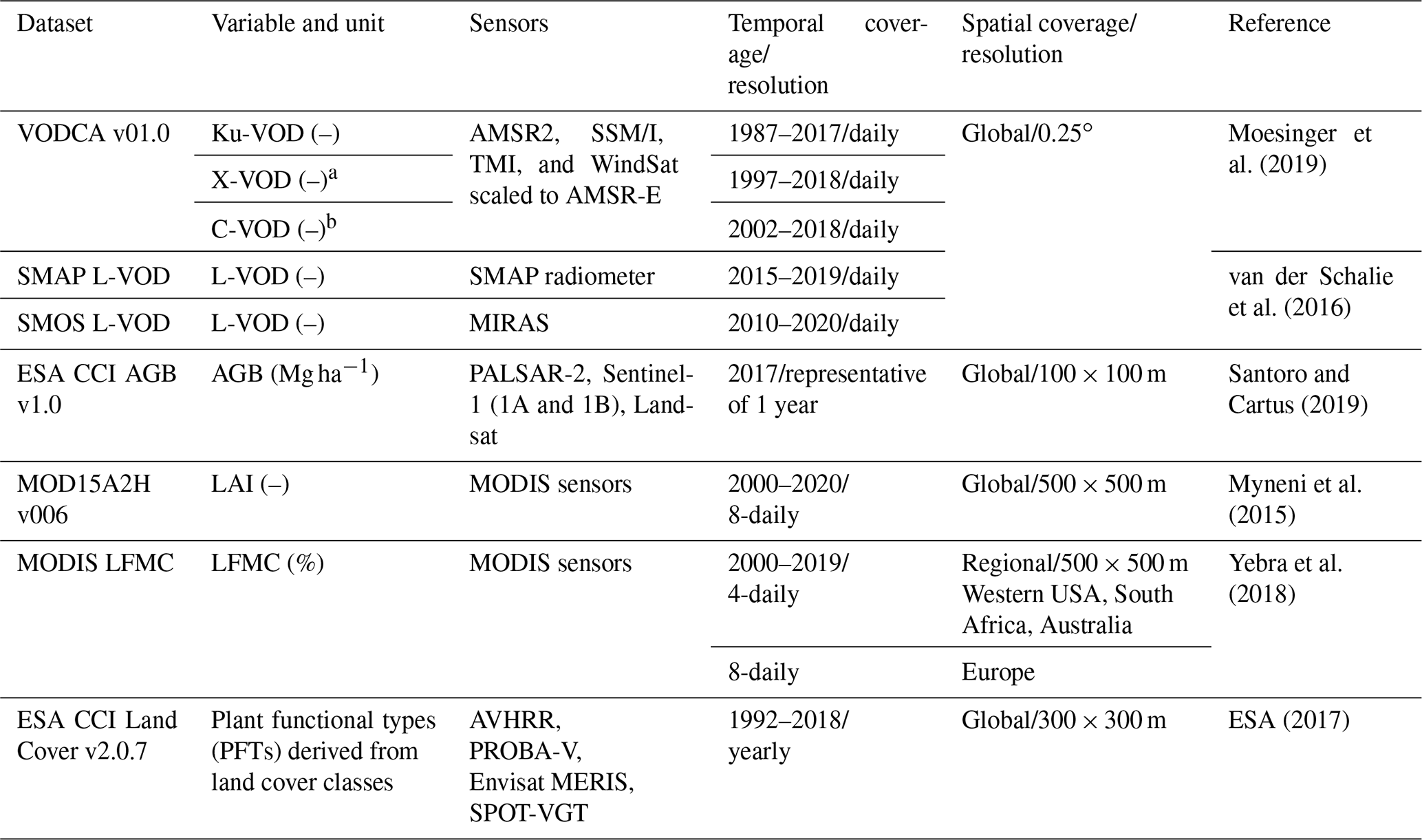
^a Does not contain SSM/I. ^b Does not contain SSM/I and TMI.

2.1.3 Data combination

All datasets were cropped to the extent of the LFMC data (Australia, Europe, western USA, South Africa) for further analyses. This implies that the “global” models as stated in the following are indeed inter-continental models restricted to the spatial extent of the LFMC dataset which mainly cover drylands except for Europe. To provide comparability of the analyses of the different VOD datasets, only the overlapping time span is used (January 2015–July 2017). The rather short time period does not impede the framework of this study because instead of analysing coherent pixel time series, this approach uses each time step of each pixel as an individual data point. The ESA CCI AGB map represents the year 2017, but we assume that the biomass does not dramatically change over 2 years. Therefore, the AGB values are kept constant for the whole time series. The PFT fractions are taken from the annual land cover maps for the respective years in 2015 to 2017 without any interpolation. During the analyses, models were trained and tested for 8-daily and monthly temporal resolutions of the LAI and LFMC time series. For the 8-daily resolution, only the VOD values matching the same timestamp of the MODIS LAI and LFMC products are used. For the monthly resolution, the mean VOD, LAI, or LFMC within the regarding month were calculated.

As a final step, pixels were excluded when the fractional coverage of bare ground or water exceeds 5 % to avoid the interpretation of marginal effects of bare soils or water on VOD. Models were specifically trained for single land cover classes. A threshold of 55 % was used to discern when a land cover class was dominant compared to the other classes.

2.2 Regression methods

To assess the influence of the vegetation variables on VOD, we applied two methods: generalized additive models (GAMs) and a random forest regressor (RF).

The RF algorithm incorporates multiple independent decision trees, where the final prediction is the average prediction of the individual trees (Breiman, 2001; Hutengs and Vohland, 2016; Liang et al., 2018). Using the scikit-learn package version 24.1 (Pedregosa et al., 2011) multiple hyper-parameters can be tuned, which will define the RF model structure. The optimization of the hyper-parameter combination is crucial to achieve a well-performing model. The scikit-learn package provides the grid-search function “RandomizedSearchCV” which enables an automatized search for an optimized parameter set by splitting the multi-variate space of the hyper-parameters into a grid of parameter combinations which are then used to train an RF. During this grid search for an exemplary dataset (predicting monthly inter-continental Ku-VOD with LAI, LFMC, AGB, and land cover), the minimum number of samples within a leaf (1 and 4), number of estimators (100 and 200–2000 with 200 steps), maximum features (functions: “auto”, “sqrt”, “log2”), maximal depth (10–110 with 20 steps and “None”), and minimum samples split (2 and 10) were tested. For a detailed description of the available hyper-parameters and their effect on the result, please refer to the documentation of the scikit-learn module sklearn.ensemble.RandomForestRegressor (https://scikit-learn.org/0.24/modules/generated/sklearn.ensemble.RandomForestRegressor.html, last access: 20 October 2022). The best combinations were again tested with monthly inter-continental predictions of X-, C-, SMOS L-VOD and SMAP L-VOD. Some combinations led to partly improved results compared to the scikit-learn default hyper-parameters but also partly degraded results. We finally selected the following hyper-parameters: minimum samples within a leaf = 1, number of estimators = 100, maximum features = “auto”, maximal depth = None, minimum samples split = 2, and criterion = mean squared error. This setup provided the best results across all tested models. The chosen maximum features parameter leads to the consideration of all features for all splits, thereby omitting one of the strengths of RF. This parameter may have been selected due to the low number of our chosen vegetation variables. However, RF is still able to capture complex relationships, which is our main focus.

GAMs are a progression of standard linear regression models and generalized linear models (GLMs) (Hastie and Tibshirani, 1987). In comparison to standard linear regression models, GLMs use a link function to connect the mean response of the target variable with the predictors, which can also represent other distributions of the target variable besides the Gaussian distribution, like binomial, gamma, or Poisson distributions (Nelder and Wedderburn, 1972). In addition, GAMs incorporate smoothing functions for each predictor variable (Yee and Mitchell, 1991). This allows for modelling non-linear and non-parametric relationships between the target and predictor variables. A general GAM equation can be written as

$$\begin{array}{}\text{(4)}& g\left(\mathit{\mu }\right)=b+\sum _{i=\mathrm{1}}^n{f}_j\left(x_i\right),\end{array}$$

with g() as the link function, μ as the mean response of target variable, b as the intercept term, f() as smoothing functions, and x as predictor variables. Thereby, g(μ) represents the target variable, i.e. predicted VOD data, and f(x_i) represents the predictors, i.e. the vegetation variables LAI, AGB, LFMC, and land cover expressed as PFT datasets. Here the GAM is developed for a Gaussian distribution with an “identity” link function and spline terms as smoothing functions using the Python package pyGAM version 0.8.0 (Servén et al., 2018).

Both methods are compared to evaluate if the relationship between the features and the target variable is additive (adequately captured by GAM) or more complex (requiring RF). GAM can represent non-linear and non-monotonic relations with single predictors whereby all predictors have a joint additive effect. RF can represent more complex relations and interactions between the single predictors but is not well suited for capturing additive structures in the data (Hastie et al., 2009). Another reason to use GAM simultaneously with RF is that models that are designed for short vegetation use just two predictors (LAI and LFMC). The AGB dataset is only representative of woody biomass of trees and can therefore not be included for short vegetation. While GAM can utilize a small number of predictors, the application of RF with only two predictors will likely result in overfitting as the random choice of a predictor variable during the development of decision trees is very limited. Both methods allow for the qualitative and quantitative assessment of the sensitivities of VOD to the predictors via accumulated local effects (ALEs; see Sect. 2.5).

2.3 Model experiments

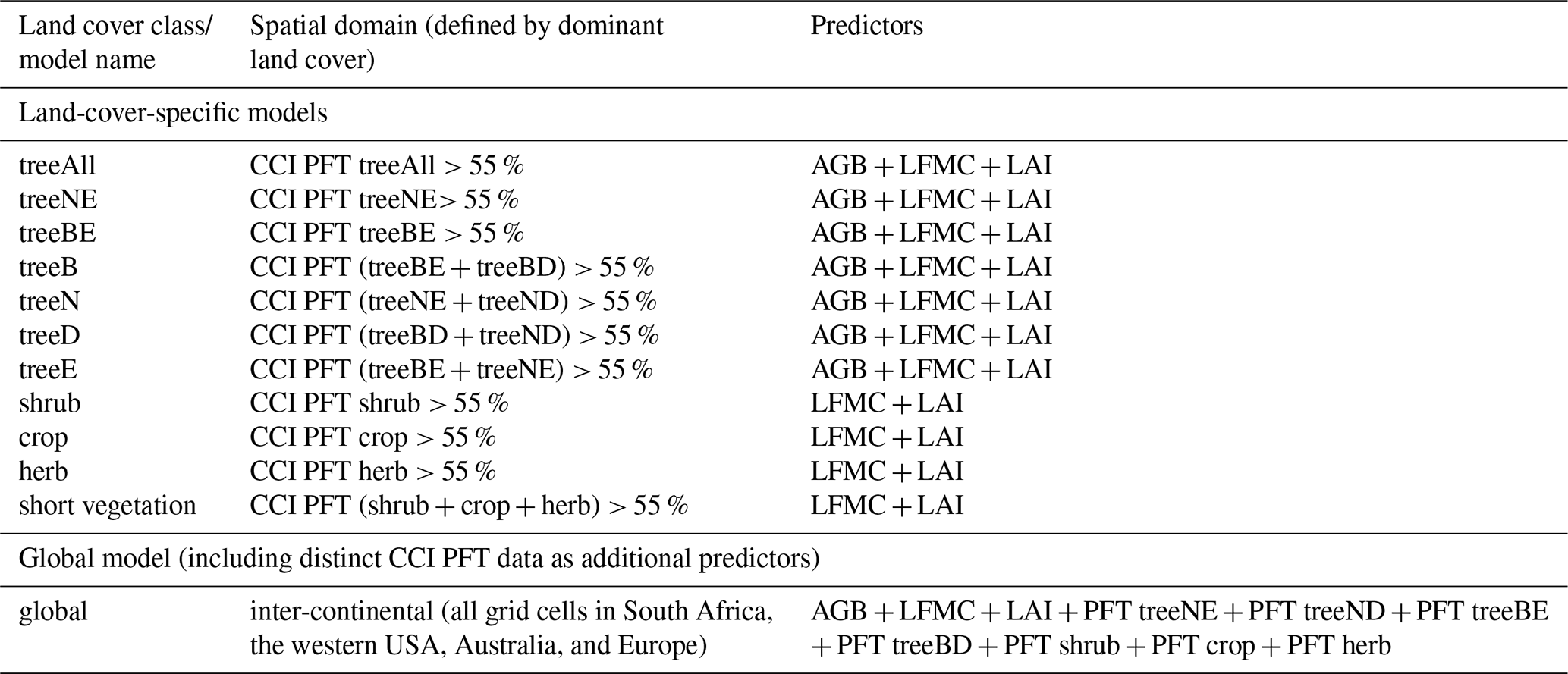
The parameter b (Eq. 2) and therefore the relationship between vegetation water content and VOD depends on the vegetation and plant type (Jackson and Schmugge, 1991). Therefore, we account for plant types by using two main classes of regression models to predict VOD. The first class is global models that use the PFTs from the land cover map in addition to the vegetation predictors LAI, LFMC, and AGB. This means that the individual maps of treeBE (broadleaf evergreen), treeBD (broadleaf deciduous), treeNE (needleleaf evergreen), treeND (needleleaf deciduous), shrub, crop, and herb are used as additional predictors. The second model class is comprised of land-cover-specific models using LAI, LFMC, and AGB as inputs. These models are only applied to the spatial extent of one dominant land cover class. In models for short-vegetation classes, AGB is not used as a predictor because this map is only representative of forest biomass. All model setups were trained both for GAM and RF and using monthly as well as 8-daily values for each VOD dataset. Table 2 gives an overview of the models and the input data. We hypothesize a better performance of global models compared to land-cover-specific models indicating that including information of the vegetation type (i.e. as a proxy for vegetation structure) in the model will improve the understanding of VOD, especially for pixels with heterogeneous land cover.

Table 2 List of tested models. N: needleleaf, B: broadleaf, E: evergreen, D: deciduous, All: not differentiated, CCI PFT: ESA Climate Change Initiative plant functional type. Each model is run with GAM and RF as well as with datasets with an 8-daily and monthly temporal resolution for each VOD dataset. The land-cover-specific models are only trained and tested within a cross-validation for pixels which are dominated by certain land cover (threshold PFT fraction > 0.55).

2.4 Model evaluation

For the evaluation of the models, 5-fold cross-validation is used. The same randomly computed folds are used for RF and GAM. The results are averages across all folds. The performance of the models is evaluated using the Nash–Sutcliffe model efficiency coefficient (NSE):

$$\begin{array}{}\text{(5)}& \mathrm{NSE}=\mathrm{1}-{\displaystyle \frac{\sum _{i=\mathrm{1}}^n{\left(a_i-b_i\right)}^{\mathrm{2}}}{\sum _{i=\mathrm{1}}^n{\left(a_i-\stackrel{\mathrm{‾}}{a}\right)}^{\mathrm{2}}}},\end{array}$$

with a as the true value, b as the predicted value, and $\stackrel{\mathrm{‾}}{a}$ as the mean of observed values as well as the root mean squared error (RMSE) between the satellite-derived and the modelled VOD. NSE commonly ranges between 1 (perfect agreement) and 0, where the latter is the score for a model which solely predicts the mean of the reference data. Models that perform worse than this can also yield negative NSE values. In addition to the overall evaluation of the models, we evaluate the spatial distribution of NSE, i.e. NSE of the satellite and modelled VOD time series.

2.5 Partial relationships: accumulated local effects (ALEs)

The relationships of VOD to the predictors are examined via accumulated local effect (ALE) plots (Apley and Zhu, 2020). Like the commonly used partial dependence plots (PDPs; Friedman, 2001), they show the marginal effect of a single predictor on the model predictions. This marginal effect is reflected in the local gradient of the ALE plot; for example, a positive gradient indicates that an increase in the investigated predictor should lead to an increase in the predicted model outcome, all other predictors being equal. While both techniques take into account all other predictors to approximate the underlying relationship with the single investigated predictor, ALE does not combine each plotted predictor value with all possible combinations of the other predictors. Especially for correlated predictors, ALE plots are therefore more robust than PDPs (Kuhn-Régnier et al., 2021), as unlikely and unrealistic feature combinations are prevented. This is achieved by defining evenly spaced quantiles across the range of the examined predictor. Each quantile is then used with only the closest existing combinations of the other predictors to calculate the marginal effects. The ALE plots were generated from the final models, where all available data were used for training. Thereby, relationships outside of the 5th and 95th percentile have to be interpreted with caution due to the smaller sample size supporting these results.

To quantify the influence of the predictors on the target variable (sensitivities), we calculated the amplitude of the ALE curve (Δ_A) as the difference between the maximum and minimum of the curve. A restriction of the ALE plots by the 5th and 95th percentile leads to slightly smaller ALE amplitudes but to the same conclusions as based on the maximum–minimum amplitude which offers the opportunity to exploit the results based on the whole data sample size.

3 Results

3.1 Performance of the models

The different regression models showed large differences in model performance in predicting VOD (−0.04 ≤ NSE ≤ 0.97; 0.004 ≤ RMSE ≤ 0.15) (Figs. 2 and S1 in Supplement). In summary, these differences were dominated by

1. the type of regression model (RF or GAM, Fig. 2 left subplots vs. right subplots, Sect. 3.1.1),

2. the use of 8-daily or monthly VOD data (symbols in Fig. 2, Sect. 3.1.2),

3. the inclusion of land cover information as a predictor (Sect. 3.1.3),

4. the wavelength of the predicted VOD (i.e. from the Ku to the L band, Sect. 3.1.4), and

5. the vegetation type to which the model is applied (Sect. 3.1.5).

Figure 2 Nash–Sutcliffe model efficiency coefficient (NSE; a, b) and RMSE (c, d) of random forest models (RF; a, c) and generalized additive models (GAM; b, d) using monthly (circle) or 8-daily (crosses) data. The global model uses PFTs as predictors, contrary to the land cover models, which were calibrated and applied only to the spatial extent of a certain dominant land cover class. Global model for short vegetation and tree cover show results of the global model but filtered by dominant land cover class.

3.1.1 Effect of the type of regression model used for calibrating the models (RF vs. GAM)

In general, RF performed better than GAM in predicting VOD, except for land-cover-specific models for short-vegetation classes where GAM reached a slightly higher NSE (Fig. 2a vs. b) and a similar RMSE compared to RF (Fig. 2c vs. d). Another exception occurs for SMOS L-VOD where GAM performed better regarding the land-cover-specific models for cropland and shrubland based on 8-daily data (see Fig. S1 for all models). While all models tended to underestimate high VOD values, RF approximated them better than GAM. Based on these findings, in the following sections, we only refer to the results of RF models. If not stated otherwise, similar results were found for GAM.

3.1.2 Effect of the temporal aggregation of the predictor variables (8-daily vs. monthly data)

Regression models based on monthly data usually exhibited a higher NSE and a lower RMSE than models based on 8-daily data (comparison of circle and crosses in Figs. 2 and S1). The superior performance of monthly over 8-daily models increased with increasing wavelength. For example, the difference was especially large for the prediction of SMOS L-VOD for which NSE doubled from 8-daily to monthly data (Fig. 2a). The performance in predicting Ku-, X-, or C-VOD was similar or monthly data presented slightly higher performance than 8-daily data. Given the higher performance of models based on monthly data, the following description of results is based on models with monthly data, unless mentioned otherwise. Section 3.2 examines the differences in VOD sensitivities to the predictors based on the considered timescale.

3.1.3 Effect of including land cover information as a predictor (global vs. land-cover-specific models)

Considering RF models based on monthly data, the global models (defined as models including fractional cover of PFTs as predictors; see Table 2) showed better model performance than the land-cover-specific models that were trained and applied only to one specific land cover. The global models performed with an NSE of 0.85 to 0.95 and an RMSE of 0.01 to 0.03 depending on VOD wavelength (Fig. 2a and c). We also compared the model performance of a specific land cover type within the global model with the related land-cover-specific model. The land-cover-specific RF models had a lower NSE (−0.09 to −0.59) and a higher RMSE (+0.006–0.03) than the global model within the same land cover. Considering GAM, land-cover-specific models performed better within a certain land cover type than the global model for the same land cover type. This applies especially for land cover types with simpler vegetation structure, e.g. shrubland, herbaceous vegetation, or broadleaf evergreen trees, and less for more complex land cover types like the tree cover and short-vegetation classes. These results indicate that the relationship between vegetation properties and VOD can be modelled with simpler relationships as represented by GAM only within a land cover type but that global relationships require more complex relationships as represented by RF.

3.1.4 Effect of wavelength

In general, the NSE of predicting short-wave VOD was higher than for predicting L-VOD and RMSE decreased from long to short wavelengths (Fig. 2). All SMOS L-VOD models performed with a lower NSE and a higher RMSE than the other VOD models including SMAP L-VOD. For RF models based on 8-daily data, NSE was highest for Ku-VOD, followed by X-VOD and C-VOD. For monthly data and GAM, the order in performance was slightly different between Ku-, X-, and C-VOD for NSE and RMSE.

In the global model, the land-cover-specific model performance depended on the different VOD wavelengths. The prediction of monthly Ku-, X-, and C-VOD using RF reached the highest performance for broadleaf evergreen trees (0.95 ≤ NSE ≤ 0.97, 0.009 ≤ RMSE ≤ 0.013) and the lowest performance for croplands (0.82 ≤ NSE ≤ 0.85, 0.015 ≤ RMSE ≤ 0.023). Predicting monthly SMAP L-VOD using RF had the highest performance in herbaceous vegetation (NSE = 0.93, RMSE = 0.016) and the lowest performance in deciduous trees (NSE = 0.74, RMSE = 0.031). RF prediction of monthly SMOS L-VOD attained the highest performance in herbaceous vegetation (NSE = 0.84, RMSE = 0.023) and the lowest performance in needleleaf and deciduous trees and croplands (NSE ∼ 0.6, 0.032 ≤ RMSE ≤ 0.059).

3.1.5 Spatial variability in model performance

The performance in predicting VOD shows large spatial differences (Fig. 3). Across all VOD datasets, the prediction of VOD was best in Australia, followed by South Africa, Europe, and the western USA (Fig. S2). As for the global model results (Sect. 3.1.4), the best performance was achieved in predicting Ku-, X-, and C-VOD, and the lowest performance was for SMOS L-VOD. This is indicated by the dominant colour distribution in Fig. 3 and by the corresponding histograms (Fig. S2), whereby the more right-skewed and narrower the distribution, the better the prediction of all pixel time series (e.g. Ku-VOD for Australia).

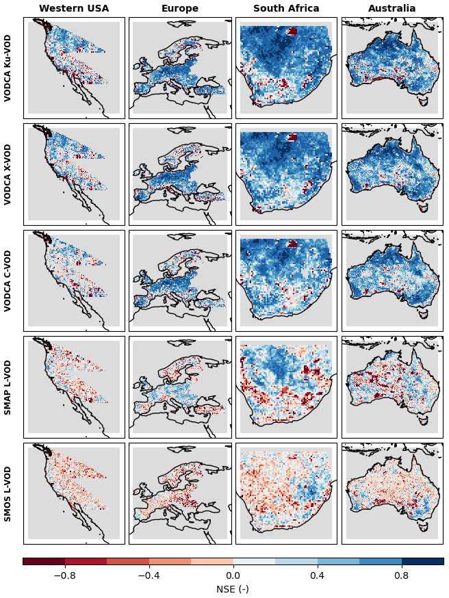
Figure 3 Nash–Sutcliffe model efficiency coefficient (NSE) per pixel for the global random forest model (PFTs included as predictor) based on monthly values. Rows indicating results for the different VOD datasets and columns indicating the different regions as dictated by the availability of the LFMC dataset. The shape of the western USA region is determined by the used h08v04, h08v05, and h09v04 MODIS tiles which form the basis for the retrieval of the LFMC data.

Several geographical patterns of high or low model performance appear for all VOD datasets. High model performance occurs mainly in regions with croplands (e.g. south-western and south-eastern Australia), large shrublands (e.g. northern Australia and central South Africa), and grasslands (north-western and south-eastern South Africa and western Australia) (high NSE, blue areas in Fig. 3). Regions in the south-western USA show a poor performance (low NSE, red areas in Fig. 3).

Higher model performance occurs also more in regions with larger seasonality in LAI and LFMC (e.g. eastern Europe and the northern part of the western USA) (Fig. 4c) and in pixels with homogenous land cover than in pixels with a more heterogeneous land cover distribution (Fig. 4a and b). With increasing wavelength, the VOD of areas with less pronounced seasonality was getting more difficult to predict.

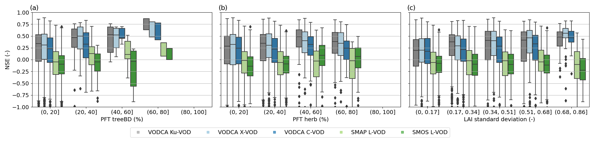
Figure 4 Spatial Nash–Sutcliffe model efficiency coefficient (NSE) based on the global random forest model computed with monthly data stratified by the land cover homogeneity of a pixel exemplary shown (a) for the tree cover class plant functional type deciduous broadleaf trees (PFT treeBD) and (b) for herbaceous vegetation (PFT herb). Note that no data with 80 %–100 % of these specific land cover classes are available. Panel (c) shows NSE stratified by the seasonality of LAI expressed as the intra-annual standard deviation of LAI. Please note that sparse data samples or even missing data result in missing boxes or whiskers.

Additionally, regions with mean VOD values less than 0.1 and marginal changes over time tend to have low or even negative NSE. This is noticeable in central Australia and central South Africa. Investigating the differences in the overall NSE based on all values (Sect. 3.1) with the grid-cell-based NSE in Figs. 3 and S3 allows for insight if the RF models are able to represent not only spatial patterns but also time series. The comparison of the high overall NSE (> 1000 data samples) with the NSE shown here (monthly time series January 2015–July 2017 resulting in a maximum time series of 31 months, i.e. <32 data samples) indicates that NSE seems to be sensitive to the data size, leading to a low NSE when few data points are available. The reference and modelled mean VOD and the variance of VOD are highly correlated in space (Spearman correlation coefficient > 0.75), which shows that the models capture the variability and spatial patterns of VOD. With a higher mean VOD the NSE increases, e.g. such as for the tree-covered areas dominated by deciduous broadleaf trees. Whereby this finding is based on the VOD range constrained by the proceeded data preparation, it might be not valid for very high VOD values, e.g. in rainforests, which are not considered here.

3.2 Relationships between VOD and vegetation properties

3.2.1 Global (inter-continental) relationships

The effects of vegetation properties on VOD for all wavelengths on a monthly or an 8-daily data basis are shown in the ALE plots in Fig. 5 (Figs. S3 and S4 for all global predictors and GAM). The amplitude Δ_A values of the ALE curves can be used as a measure of the importance of a predictor of the estimation of VOD. The amplitude Δ_A values are usually higher for monthly data than for 8-daily data (Fig. 6a), except for the relationship between AGB and SMOS L-VOD (Fig. 6c). This result indicates that the used predictors are of higher importance for monthly data than for 8-daily data. However, the high Δ_A values in the global RF model based on 8-daily data for SMOS L-VOD and the relative low performance of this model (NSE = 0.41) indicate that the influence of the used predictors might be overestimated. A predictor that could reproduce the main temporal dynamics in the 8-daily SMOS L-VOD signal is indeed missing in the analysis.

Figure 5 ALE plots of predicted normalized VOD with respect to ecosystem properties based on the global monthly or 8-daily RF model with the plant functional type (PFT) shrubland vegetation (shrub) as an example of the influence of land cover fractions on VOD. Vertical lines indicate the quantiles of the data sample sizes for 0.05, 0.25, 0.5, 0.75, and 0.95, respectively.

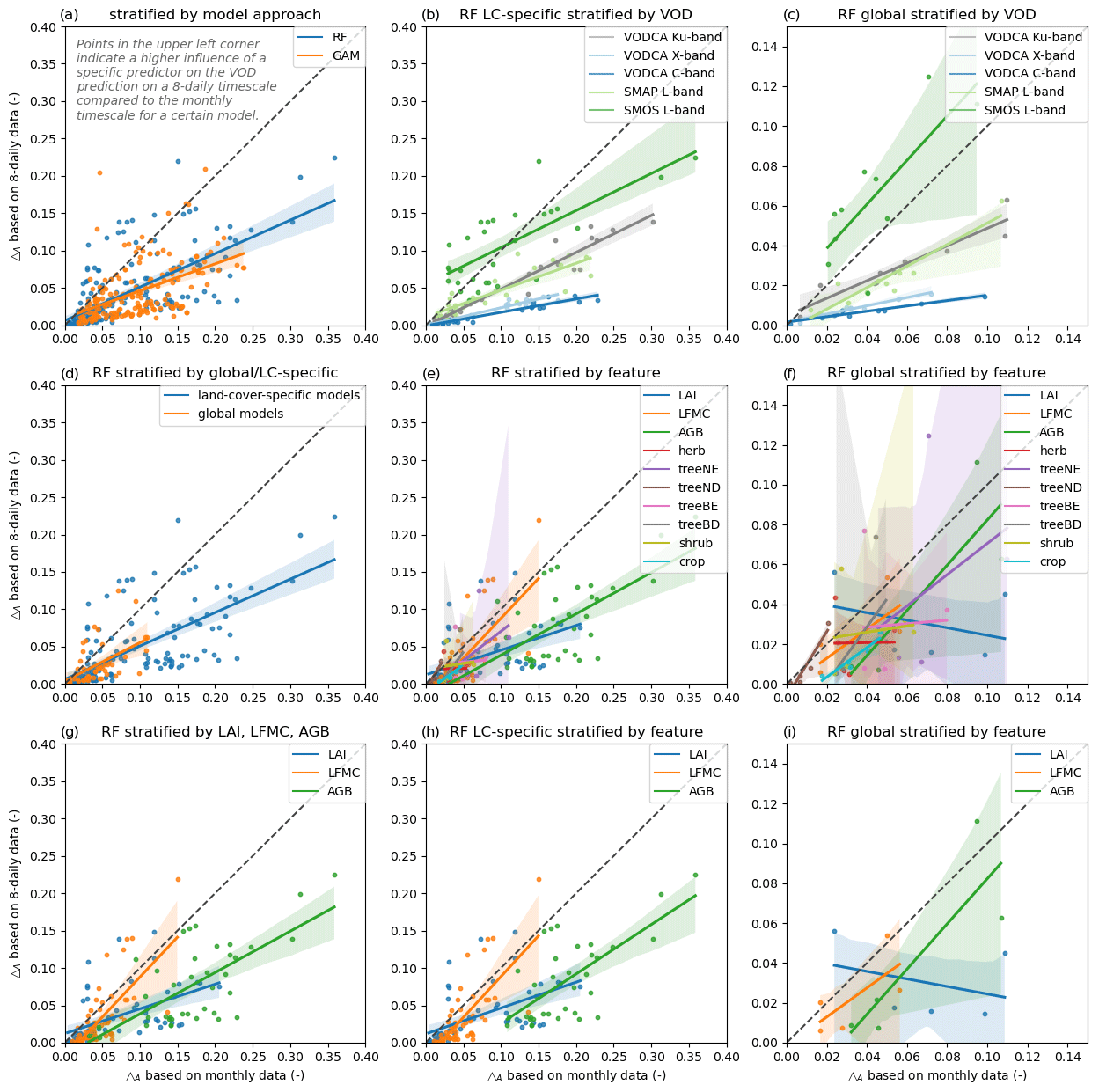
Figure 6 Regression plots of individual ALE amplitude Δ_A values on a monthly data basis vs. on an 8-daily data basis. Panel (a) shows the Δ_A of ALE curves from GAM and RF, whereby panels (b) to (i) show only Δ_A of RF models but which are colourized by different factors: “global” indicates the global models which use also PFT fractions as predictors and “LC-specific” identifies the land-cover-specific models which only use LAI, LFMC, and AGB (for tree cover) as predictors and used data filtered for the specific land cover type. Note that panels (c), (f), and (i) are zoomed in compared to the other subplots. Points located in the upper-left corner indicate a higher influence of a specific predictor on the VOD prediction on an 8-daily timescale compared to the monthly timescale for a certain model. Points located on the 1 : 1 line indicate a constant influence on VOD regardless of the considered timescale. Points located in the lower-right corner indicate a higher influence of a predictor on a monthly timescale.

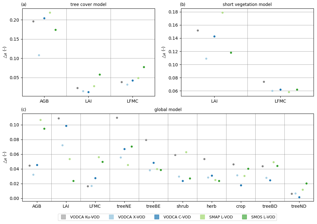
Figure 7 Amplitude (Δ_A) of RF ALEs for monthly models. The order of the x axis is solely sorted by the importance of the features while trying to ensure comparability of land-cover-specific models (a, b) and global models (c), using PFT fractions as additional predictors. Similar results are achieved for other land-cover-specific models, e.g. treeB, treeN, herb, or crop models, as well as for 8-daily based models but with a slightly smaller Δ_A.

The order of Δ_A of the predictors within a certain model are generally similar for 8-daily and monthly models. The coverages of trees are for all models one of the main contributors to the VOD predictions (Figs. 7c, S3, and S4). LAI is the second-most important predictor of Ku-VOD and the most important for X- and C-VOD. For the L-VODs the importance of LAI is lower than for the short-wave VODs (Figs. 5 and 7c). The importance of AGB increases from low to middle importance for the short-wave VODs to the highest importance for the L-VODs (Fig. 7c). The coverages of short-vegetation classes have a middle to low influence on the VOD, decreasing with increasing wavelength, but as an exception the coverages of shrubs is the second- and third-most important predictor of monthly and 8-daily SMAP L-VOD, respectively (Figs. 7c, S3 and S4). The Δ_A values of LFMC increase with wavelength, with low influence on Ku- and X-VOD and higher influence on L-VOD. An exception here is the 8-daily SMOS L-VOD model, where LFMC also has a low impact on the predictions, but given the low performance of this model, the estimated importance of LFMC on SMOS L-VOD might be unreliable (Fig. S3). Interestingly, the amplitude of the ALE plots varies between wavelengths, within monthly and 8-daily models, although these results are based on normalized data (Fig. 6c). For LAI and land cover a clear decrease in the ALE amplitude with increasing wavelength is visible, which corresponds to the fact that the magnitude of the VOD value range decreases with increasing wavelength (Figs. 5a and d and 7c). For AGB and LFMC, the ALE amplitude increases with increasing wavelength (Figs. 5b and c and 7c).

Given the similar shape of ALEs based on 8-daily and monthly data but with smaller amplitudes, we will focus on the examination of the monthly ALE curves. All VOD datasets show a positive relationship with LAI, but all curves saturate around an LAI value of 2.3, which corresponds approximately to the 95th percentile of LAI in our dataset (Fig. 5a). LAI has a much stronger effect on Ku-, X-, and C-VOD than on L-VOD. Interestingly, the relationship between LAI and SMAP L-VOD is more similar to the relationship of LAI and short-wave VODs (e.g. X-VOD) than the relationship with SMOS L-VOD (especially shown between the 75th and 95th percentile in Fig. 5a).

The relationship with LFMC is more complex for all VOD datasets (Fig. 5b). From 0 % to 50 % LFMC, the relationships are negative with a negative spike at 50 % LFMC. We hypothesize that this spike is a species-specific behaviour or a poorly captured relation for herbaceous-vegetation pixels in South Africa and Australia; however, further investigation is required to investigate if this is a real response of the vegetation. Afterwards, VOD increases with increasing LFMC, which is most pronounced for SMOS L-VOD. However, SMAP L-VOD shows a strong negative relationship with LFMC after around 140 % LFMC. Despite all relations within the 5th and 95th percentile needing to be interpreted with caution, this is especially the case for the 95th percentile of the LFMC ALE due to the uncertainties of the original dataset where higher LFMC values also have a higher uncertainty (Yebra et al., 2018). In addition, the validation of the LFMC dataset is impeded by uncertainties due to difficulties of comparison between measurements on the ground and what is detected by the satellite. Uncertainties in the used LFMC dataset arise from the temporal matching procedure of in situ samples and MODIS data and from the canopy closure of the forest cover and the contribution of the understorey to the measured surface reflectance. However, these factors are difficult to quantify and can only be discussed in a qualitative manner, but they still might influence the results presented here.

All VOD datasets show a similar increase with AGB until 120 Mg ha⁻¹ (corresponding to the 95th percentile), but the relationships differ at higher AGB values (Fig. 5c). Ku-, X-, and C-VOD show a decrease with increasing AGB above 120 Mg ha⁻¹, but SMOS and SMAP L-VOD continue to increase.

The relationships with land cover fractions are positive for most VOD datasets. As an example, we show here the relationship with the fraction of shrubland cover (Fig. 5d). SMAP L-VOD shows a nearly monotonic increase with increasing shrubland cover. The short-wave VODs and SMOS L-VOD show no relation with shrubland cover below 10 % coverage but show a positive relationship at higher coverage. SMOS L-VOD shows a non-monotonic relationship with shrubland cover.

Taken together, we find the following effects of vegetation properties on the different VOD datasets: SMOS L-VOD is most strongly affected by AGB (positive relationship), followed by tree cover and LFMC (positive relationship at LFMC > 50 %), short-vegetation cover, and LAI (positive relationship for LAI < 1.5). SMAP L-VOD is most strongly affected by AGB (positive relationship), followed by LFMC (negative relationship) and shrubland cover and LAI (positive relationship for LAI < 2.5). Ku-, X-, and C-VOD show very similar relationships and are most strongly affected by LAI (positive relationship) and tree cover, followed by AGB (positive relationship up to 120 Mg ha⁻¹), short-vegetation cover, and LFMC.

3.2.2 Relationships within land cover types

In this section, we summarize the results of the RF models for relationships within a certain land cover type (see Figs. S5 to S8 for land-cover-specific ALE plots based on RF and GAM). The individual predictors in the land-cover-specific models have a higher influence on the VOD prediction than in the global model because the land-cover-related predictors are not used within the land-cover-specific models (Fig. 6d). ALE amplitude Δ_A values for monthly data are mostly larger than for 8-daily data with some exceptions for SMOS L-VOD (Fig. 6b). The order of Δ_A for the different VODs is in the land-cover-specific models like in the global model with the highest values for SMOS L-VOD, followed by Ku- and SMAP L-VOD and X- and C-VOD.

In models for specific tree cover types, AGB has the largest Δ_A, followed by LFMC and LAI (Fig. 7a). The model for deciduous trees for 8-daily SMOS L-VOD data is an exception, in which LAI has the largest importance, followed by LFMC and AGB (Fig. S5). Due to the poor performance of this model, this result might be questionable.

Models for short-vegetation types usually have LAI as the most important predictor, followed by LFMC (Fig. 7b). Exceptions are the models for the herbaceous vegetation with 8-daily SMAP L-VOD and 8-daily and monthly SMOS L-VOD, where LFMC has the highest importance. In general, for the tree cover models AGB and for short-vegetation cover LAI have a higher influence on the predictions than LFMC. Nevertheless, the Δ_A–LFMC regression line in Fig. 6h indicates that LFMC has a similar effect on both timescales. This is contrary to AGB and LAI, where the effect is higher for monthly than for 8-daily data. For short vegetation, the ALE plot between VOD and LFMC shows a similar form as in the global model with a drop around 50 % LFMC (Fig. S6), which indicates that the global VOD–LFMC relationship is dominated by dynamics in short-vegetation areas. Particularly, the drop is based on the herbaceous land cover type, which is also visible in the 8-daily based models and in the GAM (Figs. S6 and S8). The importance of LAI in predicting VOD decreases for herbaceous and shrubland cover models with increasing wavelength. A similar dependence occurs for LFMC for shrublands and monthly data above 140 % LFMC. Globally, the positive relationship between VOD and LFMC in the range of 50 % to 140 % LFMC and the negative relationship at higher LFMC (Figs. 5b and S6) originates from croplands because this decrease is only visible in the LFMC ALE from the cropland model.

In tree-covered areas (treeAll model), the ALE shows that VOD marginally increases with LAI up to LAI = 2 and is then stable or slightly decreases (Fig. S5). The relation of VOD with LFMC is positive for Ku-, X-, and C-VOD but non-monotonic for both L-VODs. AGB is the dominant predictor of all tree-covered models, but the relationship with VOD is highly non-linear and non-monotonic, especially in comparison to the relationships with LAI and LFMC.

Comparing the ALEs of the treeAll model with the models for individual forest types (i.e. treeB, treeN, treeD, treeE, Fig. S5) shows that the influence of a specific forest type is partially recognizable within the treeAll ALEs. For example, the relationship between LFMC and VOD in the treeAll model is highly influenced by the relationship for needleleaf and evergreen trees. The decline in SMOS L-VOD with LFMC is also pronounced within most tree types but not within deciduous trees. The relationships with AGB for needleleaf trees is more linear in comparison to the other tree cover models. Deciduous and broadleaf trees exhibit a more complex relationship with AGB than evergreen and needleleaf trees for all VODs. The amplitudes of ALE curves with AGB are highest for X-VOD for deciduous trees (treeD Δ_A=0.175) and for SMOS L-VOD for broadleaf trees (treeB Δ_A=0.313). These results demonstrate that biomass is also an important predictor of short-wave VODs but that this importance varies with wavelength and forest type.

Contrary to the global model, the land-cover-specific models do not exhibit a clear dependency of the ALE amplitude on the wavelengths.

4 Discussion and conclusions

4.1 Predictors and predictability of VOD

The results demonstrate that for the global prediction of VOD, i.e. over different biomes, a flexible modelling approach such as RF is better suited than an additive approach like GAM. The lower global performance of GAM suggests that local factors, e.g. intercepted or standing water or heterogeneous soil properties, and interactions between factors play a role in the dynamics of VOD. In contrast, RF is partly able to account for this due to its ability to flexibly model, which results in higher model performance. The simpler structure of GAM compared to RF is, in most cases, insufficient to predict VOD, but within single land cover types a simpler additive approach like GAM is sufficient. This indicates that the relationship between VOD and LAI, LFMC, and AGB cannot be easily captured with global linear, monotonic, and bivariate regressions but requires accounting for the non-linear interactions between various ecosystem properties. The results imply that the set of predictors allows for the estimation of the dynamics of short-wave VODs at a high temporal resolution (8-daily and monthly) with very good performance, but the set of used predictors is insufficient to explain the dynamics in L-VOD due to ignoring local effects or possibly disregarded predictors.

This conclusion is supported by the performance difference between the four studied regions. For example, Europe has a more fragmented landscape than most areas in Australia, causing mixed effects on VOD within the coarse 0.25^∘ grid cells, leading to a lower predictability in Europe than Australia. Even if PFT fractions are used as predictors, the mismatch between the coarse resolution and land cover complexity cannot be resolved. This is especially pronounced in the long-wave VOD, for which the footprint is often significantly larger than 0.25^∘ (> 40 km). Local complex effects on VOD are likely related to land cover changes, intercepted or standing water, or soil properties. For example, Saleh et al. (2006) showed for a grassland site that intercepted water could double L-VOD after a rainfall event. Comparable to this finding, Wigneron et al. (1996) also reports a possible doubling in C-VOD due to interception at a wheat field. Although interception has reduced influence on the coarse-resolution data (Baur et al., 2019; Wigneron et al., 2021) or might not impede temporal VOD analyses (Feldman et al., 2020), temporary flooding leads to an evident change in VOD. For example, a decreased L-VOD signal at flooding was recognized for short-vegetation areas using Ku-VOD derived from the microwave radiometer of the Chinese satellite FY-3B (Fengyun) (Liu et al., 2019) as well as for forests using AMSR-E Ku-VOD (Jones et al., 2011) or using SMOS-IC L-VOD (Bousquet et al., 2021). The effect of such local events on VOD implies that large-scale spatial relations between VOD and e.g. AGB (Liu et al., 2015; Rodríguez-Fernández et al., 2018; Mialon et al., 2020) will likely wrongly associate changes in VOD with changes in AGB, which might result in unrealistic estimates of local AGB dynamics. This conclusion is supported by the findings of Konings et al. (2021), who show that regional temporal anomalies of X- and L-VOD are mostly uncorrelated with temporal anomalies of AGB but show a higher correlation with root-zone soil moisture, an indicator of water stress and availability.

The comparison of the global and the land-cover-specific models highlights the complexity of the relation between VOD and vegetation properties. An interesting result is that the ALE amplitudes (i.e. sensitivity) increase with increasing wavelength in the global model but not in the land-cover-specific model. The land-cover-specific models only include pixels with a coverage of > 55 % of the specific land cover type but do not use PFT fractions as predictors. This indicates that PFT fractions serve as a descriptor of vegetation structure and hence as a descriptor of land cover heterogeneity in the global model. This results in a VOD–LAI relationship that varies by microwave wavelength. But this wavelength dependency cannot be resolved within the land-cover-specific models because those models cannot account for the impact of sub-pixel land cover heterogeneity. Furthermore, the differences in the VOD–AGB relationship between the global and the land-cover-specific models also highlights that a monotonic VOD–AGB relationship is only valid over a large spatial scale but does not hold within a vegetation type or at smaller scales. The high model performance in regions with high biomass areas were enabled using PFT maps as predictors, which compensate for the saturating effect at high AGB. Similar to the VOD–LAI relationship, the relative sensitivity of the LFMC ALE increases with increasing wavelength for the global models, and it also shows that LFMC has relatively more influence on an 8-daily timescale compared to the monthly timescale for the global as well as the land-cover-specific models.

Both LFMC and LAI are strongly correlated. The temporal and spatial variation in our global models are dominated by LAI, leading to a lower influence of LFMC on short-wave VOD than of LAI. Although LFMC appears as the less important predictor of VOD than LAI in our models, the strong correlation of LAI and LFMC is nevertheless the reason why in situ measured LFMC show medium to strong correlations with VOD and can be used to estimate LFMC from short-wave VOD (Fan et al., 2018; Forkel et al., 2023).

Globally, the L-band VOD is highly influenced by AGB, which is in agreement with the ability of long-wave VOD to better penetrate dense vegetation and its higher sensitivity to the woody plant parts (Liu et al., 2011). However, the much lower predictability of L-VOD compared to Ku-, X-, and C-VOD indicates that L-VOD cannot be sufficiently explained by the combination of AGB, LAI, LFMC, and land cover. The performance in predicting L-VOD is much lower at the pixel level (Fig. 3) than computed across the full spatial and temporal extent of the data. Hence, the low performance in predicting L-VOD is mostly related to the temporal dynamics at the pixel level because our model correctly explains the spatial patterns. The low performance in predicting SMOS L-VOD might be caused by a noisy signal of the SMOS sensor (van der Schalie et al., 2017). Especially the daily raw L-VOD data, as used for the 8-daily analyses, can be very noisy (Wigneron et al., 2021). Vittucci et al. (2016) found moderate seasonal differences (but within the standard variation) of the SMOS L-VOD signal over forests located at latitudes higher than +20^∘, which are partly explainable due to the deciduous character of the forest but moreover because of random effects. The L-band signal, as well as the C-band signal, is strongly disturbed by radio-frequency interference (RFI; Liu et al., 2019). The spatial and temporal inconsistency of RFI complicates the RFI correction of the L band (Wigneron et al., 2021). This indicates a noisy, or until now not fully understood, variation in the SMOS L-VOD, especially within the lower value range. Due to the uncertain proportion of noise and short-term changes in water content, Ebrahimi et al. (2018) averaged SMOS L-VOD over 15 d and Rodríguez-Fernández et al. (2018) did so even over 2 years to reduce related uncertainties in the VOD signal. Vaglio Laurin et al. (2020) found a time lag of up to 6 months between SMOS L-VOD and ecosystem functional properties in tree-covered areas in South America and Africa; Tian et al. (2018) found it between SMOS L-VOD and LAI in tropical woodlands. This time lag shows that the relationships between SMOS L-VOD and vegetation properties need further investigation in densely vegetated regions.

In addition to the possible noisy signal of SMOS L-VOD, which might hamper the interpretation, errors within the L-VOD values can also be introduced by the retrieval algorithm itself. With the use of a tau-omega model, soil moisture and VOD are often retrieved simultaneously, which can introduce errors in the VOD retrievals. Zwieback et al. (2019) found spurious correlations of soil moisture and VOD especially for sub-monthly timescales over forests. Besides that, the correctness of the retrieval product focuses on soil moisture at the cost of the VOD retrieval. The resulting error shifts from soil moisture to VOD are more prone to short-term changes and to higher VOD values (Feldman et al., 2021), which might contribute to the underestimation of high VOD values of our models and the reduced performance of the 8-daily models compared to the monthly models. A more robust L-VOD product might be achieved by analysing and adjusting the necessary degree of regularization for a VOD retrieval depending on the timescale and land cover (Zwieback et al., 2019; Feldman et al., 2021).

An interesting finding is the higher sensitivity of L-VOD to LFMC than to LAI. This indicates that the L band indeed penetrates deeper into the canopy (low sensitivity to LAI) but is sensitive to the plant water status (i.e. LFMC). However, AGB and LFMC are insufficient predictors for reaching high predictability of L-VOD. This might be caused by the fact that the AGB dataset used in this study does not contain any temporal information, and hence changes in AGB are not considered in our model. Using an alternative dataset (e.g. Xu et al., 2021), which provides a global time series of AGB, could be a benefit for improving the understanding of temporal VOD variations. Especially seasonal dynamics of AGB could contribute to a better prediction of L-band VOD. However, as we included annual land cover maps as predictors, our models do indeed account for land cover change such as deforestation, which is strongly related to a change in AGB (Andela et al., 2013). The use of LFMC and LAI as predictors might be insufficient for L-VOD. The used LFMC and LAI data were both derived from optical observation by MODIS, which is only sensitive to the top of the canopy in closed forest canopies. Root-zone soil moisture was used as a proxy for water availability in other studies (e.g. Konings et al., 2021); however, it is not an ideal predictor of vegetation water content, as some plants can regulate their water potential or moisture content independent of soil moisture (Konings and Gentine, 2017; Hochberg et al., 2018). Therefore, it is necessary to further investigate the daily to seasonal temporal dynamics of L-VOD with respect to e.g. local and regional observations of water availability and plant water status.

4.2 Towards developing advanced approaches to link VOD with vegetation properties

The long time series, global coverage, and multiple frequencies of VOD retrievals provide valuable information that can be used to derive vegetation properties at large scales or to evaluate and parametrize land surface models in data assimilation studies. Yet, those applications of VOD require a solid understanding of the biophysical controls on VOD. The relatively high effect of LAI on the short-wave VODs indicates that data assimilation approaches that only use LAI for estimating the temporal dynamic of VOD (as they were used by Scholze et al., 2019, and Kumar et al., 2020) are valid approximations. However, other studies also found a relationship between short-wave VOD and plant water status (Konings et al., 2021) and negative correlation between VOD and LAI (Tian et al., 2018). This indicates that even models without an explicit representation of plant water status are suitable for VOD assimilation, but this might not hold for all vegetation types and needs further investigation.

LFMC or similar measures for plant water status have only recently been introduced into land surface models commonly used for global-scale simulations (e.g. Kennedy et al., 2019; Niu et al., 2020; Eller et al., 2020; L. Li et al., 2021). LFMC has therefore not been used in assimilation studies so far. The long time series of especially Ku-VOD could help to constrain model simulations of LFMC or support studies of plant water status but requires a good representation of LAI dynamics.

For observation operators for L-VOD, AGB should be the main predictor of spatial patterns. Scholze et al. (2019) used the empirical function between VOD and AGB evaluated by Rodríguez-Fernández et al. (2018) to simulate L-VOD from AGB. Thereby, AGB was replaced with a function of net primary production and effective turnover time. However, temporal changes in L-VOD that are caused by changes in plant water status might result in an overestimation in dynamics of biomass production, turnover, or biomass loss (Konings et al., 2021). Scholze et al. (2019) tried to avoid incorporating short-term changes in VWC and therefore averaged the VOD simulations to yearly means. The temporal dynamics should include the effect of plant water status, but further investigations on the drivers of the temporal dynamics of L-VOD are necessary to make full use of the data.

Including a proxy for VWC and exploring the influence of short-term changes in vegetation properties on VOD, we assessed the temporal dynamics not only for L-VOD but also for Ku-, X-, and C-VOD, which will help to make explicit use of VOD temporal changes within modelling and assimilation studies.