The paradox of assessing greenhouse gases from soils for nature-based solutions

Quantifying the role of soils in nature-based solutions requires accurate estimates of soil greenhouse gas (GHG) fluxes. Technological advances allow us to measure multiple GHGs simultaneously, and now it is possible to provide complete GHG budgets from soils (i.e., CO₂, CH₄, and N₂O fluxes). We propose that there is a conflict between the convenience of simultaneously measuring multiple soil GHG fluxes at fixed time intervals (e.g., once or twice per month) and the intrinsic temporal variability in and patterns of different GHG fluxes. Information derived from fixed time intervals – commonly done during manual field campaigns – had limitations to reproducing statistical properties, temporal dependence, annual budgets, and associated uncertainty when compared with information derived from continuous measurements (i.e., automated hourly measurements) for all soil GHG fluxes. We present a novel approach (i.e., temporal univariate Latin hypercube sampling) that can be applied to provide insights and optimize monitoring efforts of GHG fluxes across time. We suggest that multiple GHG fluxes should not be simultaneously measured at a few fixed time intervals (mainly when measurements are limited to once per month), but an optimized sampling approach can be used to reduce bias and uncertainty. These results have implications for assessing GHG fluxes from soils and consequently reduce uncertainty in the role of soils in nature-based solutions.

1 Introduction

Soils are essential for nature-based solutions for their role in climate mitigation potential through implementing different natural pathways (Griscom et al., 2017; Bossio et al., 2020). The climate mitigation potential of soils is dependent on multiple factors such as weather variability (Kim et al., 2012), ecosystem type (Oertel et al., 2016), soil structure (Ball, 2013), management practices (Shakoor et al., 2021), or disturbances (Vargas, 2012), where soils can ultimately act as net sources or sinks of greenhouse gases (GHGs). Therefore, accurate quantification of the magnitudes and patterns of soil GHG fluxes is needed to understand the potential of soils to mitigate or contribute to global warming across ecosystems and different scenarios.

Most of our understanding of soil GHGs has come from manual measurements performed throughout labor-intensive field campaigns and experiments (Oertel et al., 2016). While most studies around the world have focused on soil CO₂ fluxes (Jian et al., 2020), early examples have reported coupled measurements of soil CO₂, CH₄, and N₂O fluxes across tropical forests (Keller et al., 1986) and savannas (Hao et al., 1988), temperate forests (Bowden et al., 1993), and peatlands (Freeman et al., 1993). These pioneer studies not only provided an early view of the importance of integrated measurements of multiple soil GHG fluxes to understand the net global warming potential of soils but also demonstrated the technical limitations and challenges associated with these efforts. For example, it is known that manual measurements have the strength of providing good spatial coverage during field surveys but provide limited information about the temporal variability (Yao et al., 2009; Barba et al., 2021).

Technological advances have opened the opportunity to simultaneously measure multiple soil GHG fluxes (i.e., CO₂, CH₄, and N₂O) at unprecedented temporal resolution (e.g., hourly). These efforts have demonstrated differences in diel patterns and pulse events (e.g., rewetting) due to wetting and drying cycles across tropical (Butterbach-Bahl et al., 2004; Werner et al., 2007), subtropical (Rowlings et al., 2012), and temperate (Savage et al., 2014; Petrakis et al., 2017) ecosystems. These approaches provide more accurate information to calculate net GHG budgets and the global warming potential of soils (Capooci et al., 2019). That said, performing automated measurements of multiple GHGs is expensive, and this approach usually has a lower representation of the spatial heterogeneity within ecosystems (Yao et al., 2009; Barba et al., 2021).

Ideally, we would like to measure everything, everywhere, and all the time, but this is impossible due to logistical, technological, physical, and economic constraints. Lightweight and low-powered laser-based spectrometers have reduced technical barriers to simultaneously measuring multiple GHG fluxes from soils. It is now easier and faster to perform discrete manual surveys across time. This opportunity creates a paradox concerning when to measure different GHG fluxes from soils when performing manual measurements. Researchers generally tend to perform simultaneous measurements of multiple GHGs during manual surveys, but this convenience could result in biased information. We propose that there is a conflict between the convenience of measuring multiple GHGs at a few fixed time intervals and the intrinsic temporal variability in magnitudes and patterns of different GHG fluxes.

Here, we present a proof of concept and test how a subset of measurements derived from a fixed temporal stratification (FTS) for simultaneous measurements (i.e., stratified sampling schedule) or using an optimized sampling (i.e., temporal univariate Latin hypercube sampling, tuLHs) compared with automated measurements of soil CO₂ (F_ACO₂), CH₄ (F_ACH₄), and N₂O (F_AN₂O) fluxes from a temperate forest (Petrakis et al., 2018; Barba et al., 2021, 2019). The underlying assumption supporting any FTS approach is that a few measurements in time can reproduce the statistical properties and temporal dependencies of soil CO₂, CH₄, and N₂O fluxes because these GHGs respond similarly to biological and physical drivers. The tuLHs is a new statistical method for generating subsamples of parameter values (i.e., soil GHG gas fluxes in this case study) to reproduce the probability distribution and the temporal dependence of each original time series of GHG fluxes. We reveal that reporting GHG fluxes using an FTS for simultaneous measurements may result in biased information on temporal patterns and magnitudes. This study shows how a biased sampling schedule could influence our understanding of GHG fluxes and, ultimately, the climate mitigation potential of soils.

2 Materials and methods

2.1 Study site

The experiment was performed in a temperate forest located at the St Jones Reserve (a component of the Delaware National Estuarine Research Reserve (DNERR) in Delaware, USA). The site has a mean annual temperature of 13.3 ^∘C and mean annual precipitation of 1119 mm. Soils are classified as Othello silt loam with a texture of 40 % sand, 48 % silt, and 12 % clay within the first 10 cm (Petrakis et al., 2018). The dominant plant species are bitternut hickory (Carya cordiformis), eastern red cedar (Juniperus virginiana L.), American holly (Ilex opaca), sweetgum (Liquidambar styraciflua L.), and black gum (Nyssa sylvatica (Marshall)). The site has a mean tree density of 678 stems ha⁻¹ and a diameter at breast height (DBH) of 25.7 ± 13.9 cm (mean ± SD) (Barba et al., 2021).

2.2 Automated measurements of soil GHG fluxes

We analyzed data from automated measurements (1 h time intervals) of soil emissions of three GHGs (i.e., CO₂, CH₄, and N₂O) between January and December 2015. This was a typical year with a mean annual temperature of 13.4 ^∘C and annual precipitation of 1232 mm. Continuous measurements of soil GHGs were taken by coupling a closed-path infrared gas analyzer (LI-COR LI-8100A, Lincoln, Nebraska) and nine dynamic soil chambers (LI-COR 8100-104) controlled by a multiplexer (LI-COR 8150) with a cavity ring-down spectrometer (Picarro G2508, Santa Clara, California). A detailed description of the experimental design and measurement protocol has been described in previous studies (Petrakis et al., 2018; Barba et al., 2021, 2019). Briefly, for each flux observation, we measured CO₂, CH₄, and N₂O concentrations every second with the Picarro G2508 for 300 s and calculated fluxes (at 1 h time intervals) from the mole dry fraction of each gas (i.e., corrected for water vapor dilution) using the SoilFluxPro software (v4.0; LI-COR, Lincoln, Nebraska, USA). Fluxes were estimated using linear and exponential fits, and we kept the flux calculation with the highest R². We applied quality assurance and quality control protocols using information from all three GHGs as established in previous studies (Petrakis et al., 2018, 2017; Barba et al., 2021, 2019; Capooci et al., 2019). Using these time series, we extracted values to represent discrete temporal measurements based on FTS and used the optimization approach described below.

2.3 Temporal subsampling of time series

Subsampling of time series was performed using FTS and a temporal optimization following a univariate Latin hypercube (tuLHs) approach. The difference between FTS and temporal optimization is that the first approach is focused on a fixed schedule (e.g., sampling once per month) and the second is focused on reproducing the statistical properties and temporal dependence relationship of the original GHG time series with a subset of measurements. This means optimized subsamples may not be spaced systematically (e.g., every 15 d), and selected dates may vary for each GHG flux due to their specific statistical properties and temporal dependence.

FTS represents a traditional schedule for performing manual measurements of GHG fluxes from soils. The FTS is usually performed with manual measurements because they require extensive logistical coordination due to travel time and costs, availability of instrumentation (e.g., gas analyzers), personnel to perform the measurements, and weather conditions. During these scheduled visits, researchers usually collect fluxes from all three GHGs and analyze them systematically to calculate magnitudes and patterns throughout the experiment. Usually, researchers perform manual samples during the early hours of the day (between 09:00 and 12:00 LT) to avoid confounding effects due to large changes in temperature and moisture, as demonstrated by information summarized by the soil respiration global database (Cueva et al., 2017; Jian et al., 2020). Consequently, we selected subsamples from each original GHG time series (derived from automated measurements) using flux measurements from 10:00 LT at fixed intervals of once per month (n = 12), twice per month (n = 24), or four times per month (n = 48) starting from the first week of available data from automated measurements.

We applied tuLHs as an alternative subsampling approach to obtain an optimized subsample with the same univariate statistical properties and temporal dependence relationship as the original GHG time series. Optimization was performed to select subsamples for each GHG flux using the same number of samples as for FTS: 12 (k = 12), 24 (k = 24), or 48 (k = 48) measurements throughout the year of available data from automated measurements.

2.4 Temporal univariate Latin hypercube sampling (tuLHs)

Let $S=\mathit{\left\{}\right(x_{\mathrm{1}},y_{\mathrm{1}},z_{\mathrm{1}}),(x_{\mathrm{2}},y_{\mathrm{2}},z_{\mathrm{2}}),\mathrm{\dots },(x_n,y_n,z_n\left)\mathit{\right\}}$ be observations of the variables X, Y, and Z in a time series, where X, Y, and Z are soil GHGs (i.e., CO₂, CH₄, and N₂O). Each measured variable is characterized by the univariate probability distribution function and the temporal dependency function. Once these two functions are known, then the behaviors of the variable can be reproduced (Le et al., 2020; Chilès and Delfiner, 2009; Trangmar et al., 1986; Pyrcz and Deutsch, 2014). The tuLHs consists of three steps: (1) modeling the univariate behavior of the variable using the empirical cumulative univariate probability distribution function; (2) modeling the temporal dependence using the empirical variogram function; and (3) optimizing a subsample applying a global optimization method, differential evolution, using the previously obtained variogram function as an objective function.

First, to model the univariate behavior of the variables from the observations of S, the empirical univariate cumulative distribution function $F_n^{\ast }\left(x\right)$ of X is estimated by

$$\begin{array}{}\text{(1)}& F_n^{\ast }\left(x\right)={\displaystyle \frac{\mathrm{1}}{n}}\sum _{i=\mathrm{1}}^{n}I{x}_i\le x\mathrm{8},\end{array}$$

where I represents an indicator function equal to 1 when its argument is true and is 0 otherwise. Similarly, the empirical univariate distribution function of the variables Y and Z can be derived.

Second, to model the temporal dependence of the variables from the observations of S, the empirical temporal correlation function (i.e., temporal variogram function) γ^∗(t) of X is estimated by

$$\begin{array}{}\text{(2)}& {\mathit{\gamma }}^{\ast }\left(t\right)={\displaystyle \frac{\mathrm{1}}{\mathrm{2}N\left(t\right)}}\sum _{i=\mathrm{1}}^{N\left(t\right)}\left[X\right(t_i+t)-X(t_i){]}^{\mathrm{2}},\end{array}$$

where N(t) is the number of pairs and X(t_i+t) and X(t_i) are separated by a time t. The variogram functions of the variables Y and Z are analogous. Third, to optimize the subsample, it is required to choose the “optimal” data points with the selected sample size (i.e., k = 12, 24, or 48, where k≪n) that will have the same behavior as the original observations of S (i.e., GHG fluxes derived from automated measurements). To achieve this objective, we use differential evolution, a global optimization method (Storn and Price, 1997), using the variogram function as an objective function. The procedure consists of dividing the univariate empirical probability distribution in Eq. (1) into k equiprobable strata, which is equivalent to k-ordered data subsets. From each subset, only one value must be chosen to satisfy the condition of a univariate Latin hypercube. The differential evolution method is applied to find the optimal points that minimize the difference between the subsample variogram γ(t) and the data variogram γ^∗(t) in Eq. (3).

$$\begin{array}{}\text{(3)}& {\text{OF}}_{\mathrm{1}}=\sum _{i=\mathrm{1}}^{N\left(t\right)}\left[\mathit{\gamma }\right(t)-{\mathit{\gamma }}^{\ast }(t){]}^{\mathrm{2}},\end{array}$$

where OF is the objective function and the variograms γ(t) and γ^∗(t) are calculated using Eq. (2).

2.5 Statistical analyses

The t test was used to compare the means, and the Kolmogorov–Smirnov test was used to compare the probability distribution of measurements derived from each sampling protocol. All tests were performed with a 95 % confidence level. In addition, their statistical properties, such as the mean, median, standard deviation, and first and third quartiles, were compared. The differences in the experimental semivariograms were calculated as a comparison measure for the temporal dependence of the samples and the original time series of GHG fluxes. For cumulative sums of GHG flux, their mean is calculated as the most likely value, and their quantile difference between 97.5 % and 2.5 % is used to quantify the range of uncertainty. All analyzes were performed using the R program (R Code Team, 2013).

3 Results

3.1 Relationships among GHG fluxes from soils

Justification in support of FTS for simultaneous measurements of GHG fluxes would require evidence of strong linear correlations between magnitudes and temporal dependence among soil GHG fluxes. First, we did not find strong linear relationships between any combination of GHG fluxes from soils derived from automated measurements (Fig. S1 in the Supplement). Therefore, our data did not support the assumption that the magnitude of one GHG flux was associated with a linear increase or decrease in another GHG flux. Second, semivariogram models demonstrated differences in the temporal dependence for each GHG flux. Automated measurements of soil CO₂ fluxes (F_ACO₂) showed a temporal dependence following a Gaussian variogram model, with a nugget of 4, a sill plus nugget of 28, and a correlation range of 80 d (Fig. S2a). Automated measurements of soil CH₄ fluxes (F_ACH₄) also showed a temporal dependence but followed a spherical variogram model, with a nugget of 7 × 10⁻⁸, a sill plus nugget of 1.5 × 10⁻⁷, and a correlation range of 110 d (Fig. S2b). In contrast, automated measurements of soil N₂O fluxes (F_AN₂O) did not show a temporal dependence, where a pure nugget effect was present and with a correlation range of 0 d (Fig. S2c). Consequently, these GHG fluxes' magnitudes and temporal patterns were different and did not support FTS for simultaneous measurements of GHG from soils.

3.2 Optimization of GHG sampling protocols

We applied a tuLHs approach to identify subsamples with the same statistical properties and temporal dependence for each of the original GHG time series from automated measurements. Subsamples were identified for 12 (k = 12), 24 (k = 24), or 48 (k = 48) measurements throughout the year for each GHG time series. Our results show that the optimized measurement dates were different for each GHG flux (Fig. 1), and we provide explicit examples for k = 24 (Fig. 1) and k = 12 and 48 (Figs. S3 and S4).

The optimized CO₂ subsamples were well distributed throughout the year for all sampling scenarios (i.e., k from 12 to 48) because F_ACO₂ had a strong temporal dependence and a small nugget effect with respect to the sill (Fig. S2a). The optimized CH₄ subsamples were also relatively well distributed throughout the year, especially for scenarios of k = 24 and k = 48, as F_ACH₄ also had a temporal dependence but with a higher nugget effect with respect to the sill (Fig. S2b). Finally, the optimized N₂O subsamples were more challenging to define, especially with a small sample size (i.e., k = 12; Fig. S3c) because F_AN₂O did not have a temporal dependence (Fig. S2c).

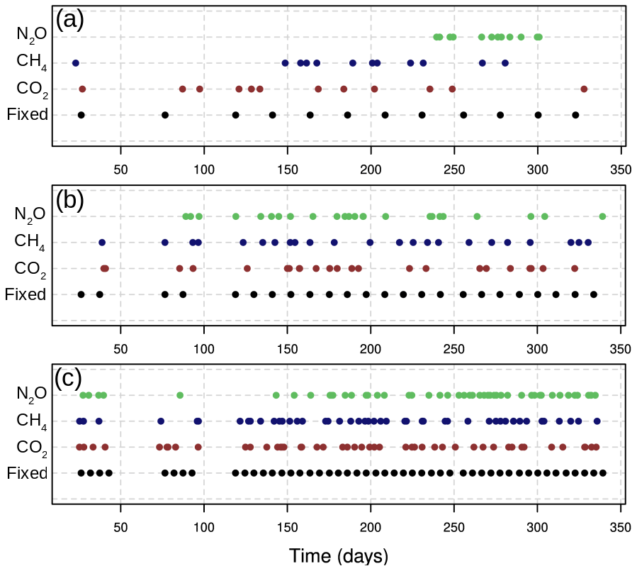
Figure 1 Temporal distribution of fixed temporal stratification (i.e., stratified manual sampling approach) and optimized sampling using a temporal univariate Latin hypercube (tuLHs) approach for k = 12 (a), k = 24 (b), and k = 48 (c). Fixed temporal stratification is in black, soil CO₂ fluxes in red, soil CH₄ fluxes in blue, and soil N₂O fluxes in green. Time (x axis) represents days from 1 January to 31 December 2015.

3.3 Differences in statistical properties and temporal dependency of subsamples

Overall, there were no statistically significant differences between the mean values derived from automated measurements and those from FTS or the tuLHs approach (Fig. 2 for k = 24; Fig. S5 for k = 12; Fig. S6 for k = 48; Tables S1 and S2 in the Supplement). Although this appears promising, more than a simple comparison of the means is needed to evaluate the information derived from different sampling approaches. In other words, it is possible to have a similar mean value without reproducing the probability distribution or the temporal dependence of the original time series (i.e., correct answer but for the wrong reasons). Here, we present results based on comparing the means, standard deviation, probability distributions, and semivariograms derived from automated measurements and the different sampling scenarios for all GHG fluxes.

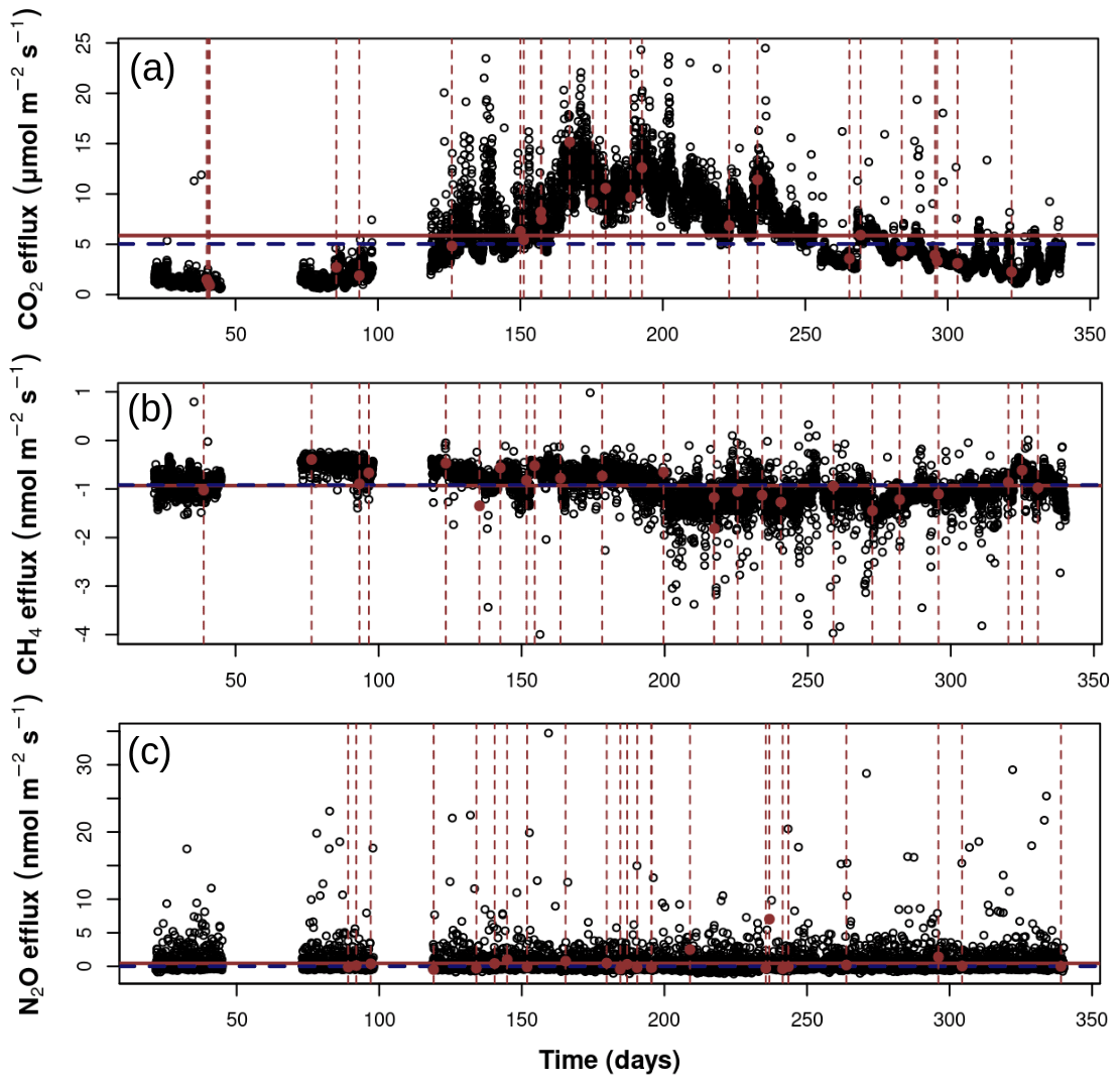
Figure 2 Time series of automated measurements (F_A) of soil greenhouse gas fluxes (black circles) and optimized samples (k = 24) using a temporal univariate Latin hypercube sampling (tuLHs) approach for soil CO₂ (a), soil CH₄ (b), and soil N₂O (c) fluxes. The horizontal red line represents the mean, and the horizontal blue line is the median of each greenhouse gas flux derived from automated measurements. The selection of data points for k = 12 and 48 is presented for each soil greenhouse gas time series in Figs. S3 and S4, respectively. Time (x axis) represents days from 1 January to 31 December 2015.

The mean of F_ACO₂ was 5.9 $\mathrm{\mu }\mathrm{mol}{\mathrm{CO}}_{\mathrm{2}}{\mathrm{m}}^{-\mathrm{2}}{\mathrm{s}}^{-\mathrm{1}}$, while the mean for FTS was 5.5 and 5.9 $\mathrm{\mu }\mathrm{mol}{\mathrm{CO}}_{\mathrm{2}}{\mathrm{m}}^{-\mathrm{2}}{\mathrm{s}}^{-\mathrm{1}}$ for the tuLHs approach with k = 24 (Fig. 3a–c). These results were comparable with the means derived from FTS (5.4 and 5.4 $\mathrm{\mu }\mathrm{mol}{\mathrm{CO}}_{\mathrm{2}}{\mathrm{m}}^{-\mathrm{2}}{\mathrm{s}}^{-\mathrm{1}}$) and the tuLHs approach (6.2 and 5.9 $\mathrm{\mu }\mathrm{mol}{\mathrm{CO}}_{\mathrm{2}}{\mathrm{m}}^{-\mathrm{2}}{\mathrm{s}}^{-\mathrm{1}}$) using k = 12 and k = 48, respectively (Figs. S5 and S6; Table S1). The standard deviation of F_ACO₂ was 3.9 and 3.2 $\mathrm{\mu }\mathrm{mol}{\mathrm{CO}}_{\mathrm{2}}{\mathrm{m}}^{-\mathrm{2}}{\mathrm{s}}^{-\mathrm{1}}$ for FTS and 3.9 $\mathrm{\mu }\mathrm{mol}{\mathrm{CO}}_{\mathrm{2}}{\mathrm{m}}^{-\mathrm{2}}{\mathrm{s}}^{-\mathrm{1}}$ for the tuLHs approach with k = 24 (Fig. 3a–c). These results were comparable with the standard deviations derived from FTS (3.1 and 3.3 $\mathrm{\mu }\mathrm{mol}{\mathrm{CO}}_{\mathrm{2}}{\mathrm{m}}^{-\mathrm{2}}{\mathrm{s}}^{-\mathrm{1}}$) and the tuLHs approach (4.1 and 3.9 $\mathrm{\mu }\mathrm{mol}{\mathrm{CO}}_{\mathrm{2}}{\mathrm{m}}^{-\mathrm{2}}{\mathrm{s}}^{-\mathrm{1}}$) using k = 12 and k = 48, respectively (Figs. S5 and S6; Table S1). Our results show that the semivariograms of optimized samples using the tuLHs approach closely approximate the semivariograms of automated measurements for k = 24 (Fig. 4a) and k = 12 and 48 (Figs. S7a and S8a). These results are consistent with the sums of absolute differences between the semivariograms of the samples and the semivariogram of F_ACO₂ with differences of 69.31, 54.39, and 49.42 for FTS and of 5.69, 1.99, and 1.39 for the tuLHs approach for k = 12, 24, and 48, respectively (Table S2).

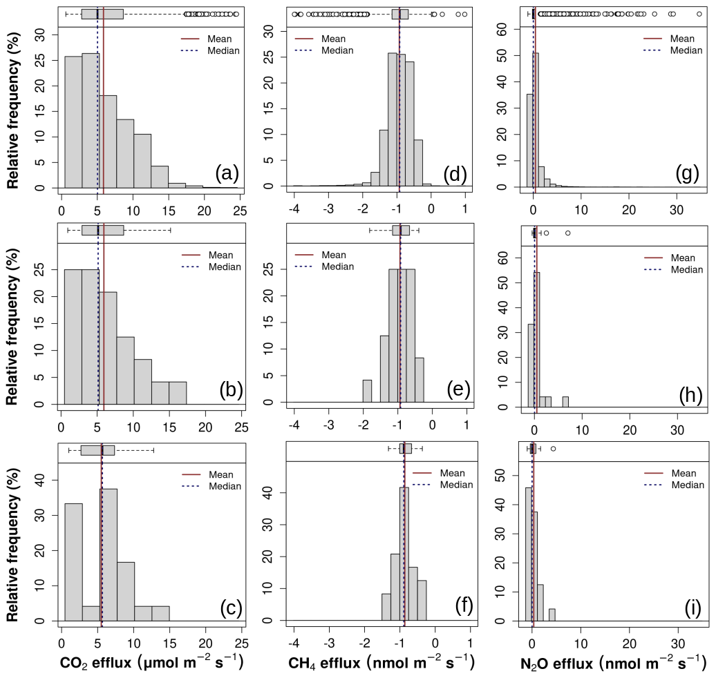
Figure 3 Histograms for automated measurements of soil CO₂ (F_A CO₂; a), soil CH₄ (F_A CH₄; d), and soil N₂O (F_A N₂O; g). Histograms for optimized samples (k = 24) using a temporal univariate Latin hypercube sampling (tuLHs) approach for soil CO₂ (b), soil CH₄ (e), and soil N₂O (h) fluxes. Histograms for fixed temporal stratification (i.e., stratified manual sampling schedule) (k = 24) for soil CO₂ (c), soil CH₄ (f), and soil N₂O (i) fluxes. The Supplement includes results for measurements with k = 12 (Fig. S5) and k = 48 (Fig. S6).

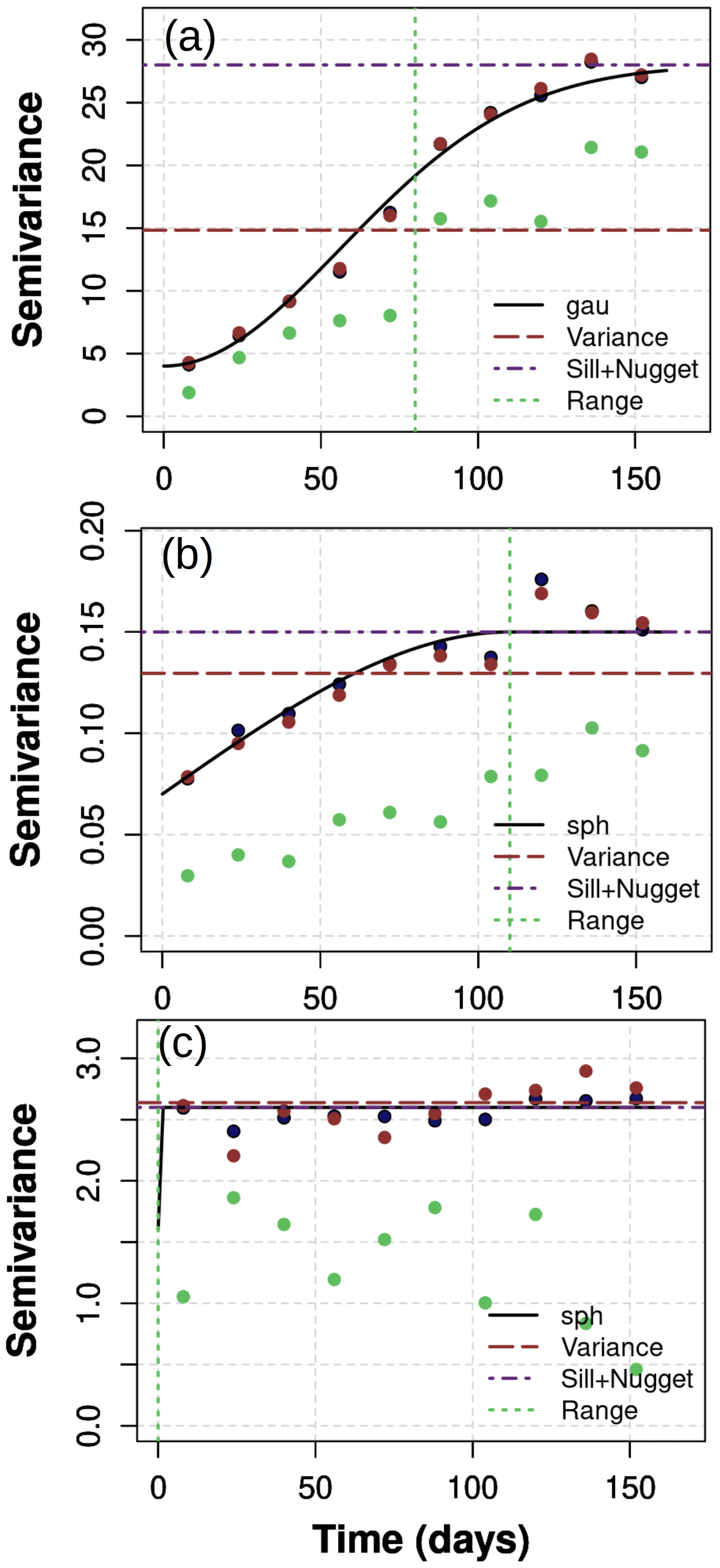
Figure 4 Comparison of semivariograms between automated measurements (F_A) of soil greenhouse gas fluxes (solid black line) and for optimized samples using a temporal univariate Latin hypercube sampling (tuLHs) approach (red circles) or fixed temporal stratification (green circles) with k = 24. Semivariograms are presented for soil CO₂ (a), CH₄ (b), and N₂O (c) fluxes. Semivariograms for measurements with k = 12 and k = 48 are shown in Figs. S7 and S8, respectively. Semivariogram fits were Gaussian (gau) or spherical (sph).

The mean of F_ACH₄ was −0.93 $\mathrm{nmol}{\mathrm{CH}}_{\mathrm{4}}{\mathrm{m}}^{-\mathrm{2}}{\mathrm{s}}^{-\mathrm{1}}$, while it was −0.86 $\mathrm{nmol}{\mathrm{CH}}_{\mathrm{4}}{\mathrm{m}}^{-\mathrm{2}}{\mathrm{s}}^{-\mathrm{1}}$ for FTS and −0.94 $\mathrm{nmol}{\mathrm{CH}}_{\mathrm{4}}{\mathrm{m}}^{-\mathrm{2}}{\mathrm{s}}^{-\mathrm{1}}$ for the tuLHs approach with k = 24 (Fig. 3d–f). These results were also comparable with the means derived from FTS (−0.83 and −0.88 $\mathrm{nmol}{\mathrm{CH}}_{\mathrm{4}}{\mathrm{m}}^{-\mathrm{2}}{\mathrm{s}}^{-\mathrm{1}}$) and the tuLHs approach (−0.87 and −0.92 $\mathrm{nmol}{\mathrm{CH}}_{\mathrm{4}}{\mathrm{m}}^{-\mathrm{2}}{\mathrm{s}}^{-\mathrm{1}}$) using k = 12 and 48, respectively (Figs. S5 and S6; Table S1). The standard deviation of F_ACH₄ was 0.36 and 0.26 $\mathrm{nmol}{\mathrm{CH}}_{\mathrm{4}}{\mathrm{m}}^{-\mathrm{2}}{\mathrm{s}}^{-\mathrm{1}}$ for FTS and 0.34 $\mathrm{nmol}{\mathrm{CH}}_{\mathrm{4}}{\mathrm{m}}^{-\mathrm{2}}{\mathrm{s}}^{-\mathrm{1}}$ for the tuLHs approach with k = 24. These results were comparable with the standard deviations derived from FTS (0.27 and 0.29 $\mathrm{nmol}{\mathrm{CH}}_{\mathrm{4}}{\mathrm{m}}^{-\mathrm{2}}{\mathrm{s}}^{-\mathrm{1}}$) and the tuLHs approach (0.33 and 0.35 $\mathrm{nmol}{\mathrm{CH}}_{\mathrm{4}}{\mathrm{m}}^{-\mathrm{2}}{\mathrm{s}}^{-\mathrm{1}}$) using k = 12 and k = 48, respectively (Figs. S5 and S6; Table S1). The semivariograms of optimized samples using the tuLHs approach closely approximate the semivariogram of automated measurements for k = 24 (Fig. 4b) and k = 12 and 48 (Figs. S7b and S8b). Consequently, the sums of absolute differences between the semivariograms of the samples and the semivariogram of F_ACH₄ were 0.63, 0.48, and 0.49 for FTS and 0.06, 0.04, and 0.02 for the tuLHs approach with k = 12, 24, and 48, respectively (Table S2).

Finally, the mean of F_AN₂O was 0.45 and 0.61 $\mathrm{nmol}{\mathrm{N}}_{\mathrm{2}}\mathrm{O}{\mathrm{m}}^{-\mathrm{2}}{\mathrm{s}}^{-\mathrm{1}}$ for FTS and 0.51 $\mathrm{nmol}{\mathrm{N}}_{\mathrm{2}}\mathrm{O}{\mathrm{m}}^{-\mathrm{2}}{\mathrm{s}}^{-\mathrm{1}}$ for the tuLHs approach with k = 24 (Fig. 3g–i). These results were also comparable with the means derived from FTS (0.59 and 0.25 $\mathrm{nmol}{\mathrm{N}}_{\mathrm{2}}\mathrm{O}{\mathrm{m}}^{-\mathrm{2}}{\mathrm{s}}^{-\mathrm{1}}$) and the tuLHs approach (0.58 and 0.49 $\mathrm{nmol}{\mathrm{N}}_{\mathrm{2}}\mathrm{O}{\mathrm{m}}^{-\mathrm{2}}{\mathrm{s}}^{-\mathrm{1}}$) using k = 12 and 48, respectively (Figs. S5 and S6; Table S1). The standard deviation of F_AN₂O was 1.62 and 1.97 $\mathrm{nmol}{\mathrm{N}}_{\mathrm{2}}\mathrm{O}{\mathrm{m}}^{-\mathrm{2}}{\mathrm{s}}^{-\mathrm{1}}$ for FTS and 1.54 $\mathrm{nmol}{\mathrm{N}}_{\mathrm{2}}\mathrm{O}{\mathrm{m}}^{-\mathrm{2}}{\mathrm{s}}^{-\mathrm{1}}$ for the tuLHs approach with k = 24. These results were comparable with the standard deviations derived from FTS (1.38 and 0.91 $\mathrm{nmol}{\mathrm{N}}_{\mathrm{2}}\mathrm{O}{\mathrm{m}}^{-\mathrm{2}}{\mathrm{s}}^{-\mathrm{1}}$) and the tuLHs approach (1.58 and 1.54 $\mathrm{nmol}{\mathrm{N}}_{\mathrm{2}}\mathrm{O}{\mathrm{m}}^{-\mathrm{2}}{\mathrm{s}}^{-\mathrm{1}}$) using k = 12 and k = 48, respectively (Figs. S5 and S6; Table S1). Our results show no temporal dependence for N₂O fluxes, but the semivariograms of optimized samples using the tuLHs approach closely approximate the semivariogram of automated measurements for k = 24 (Fig. 4c) and k = 12 and 48 (Figs. S7c and S8c). Consistently, the sum of absolute differences between the semivariograms of the samples and the semivariogram of F_AN₂O was 10.01, 12.25, and 16.75 for FTS and 0.82, 1.13, and 3.57 for the tuLHs approach with k = 12, 24, and 48, respectively (Table S2).

These results show that the tuLHs approach reproduced the probability distribution and the temporal dependence of the time series derived from automated measurements with more precision than FTS for all GHGs. In the next section, we explore the implications of these differences for calculating cumulative GHG fluxes.

3.4 Calculation of cumulative GHG fluxes

We calculated the cumulative flux for all GHGs using available information from automated measurements (Fig. 2; Table S3). The cumulative sum for available measurements for F_ACO₂ was 5758.5 g CO₂ m⁻² ([893.9, 13860.8], 95 %  CI), for F_ACH₄ was −0.47 g CH₄ m⁻² ([−0.81, −0.19], 95 %  CI), and for F_AN₂O was 0.63 g N₂O m⁻² ([−0.75, 5.19], 95 %  CI).

We used the mean for each GHG flux derived from the tuLHs approach or the FTS to calculate the cumulative sum (Table S3). We found that the FTS underestimated the cumulative flux (−8.4 %, −6.2 %, −7.1 %) and the uncertainty (−32.6 %, −21.6 %, −19.3 %) of F_ACO₂ for k = 12, 24, and 48, respectively (Fig. 5a). In contrast, the tuLHs approach slightly overestimated the cumulative flux (6.5 %, 1.1 %, 0.1 %) and slightly underestimated the uncertainty (−9.1 %, −4.4 %, −3.7 %) for k = 12, 24, and 48, respectively (Fig. 5a).

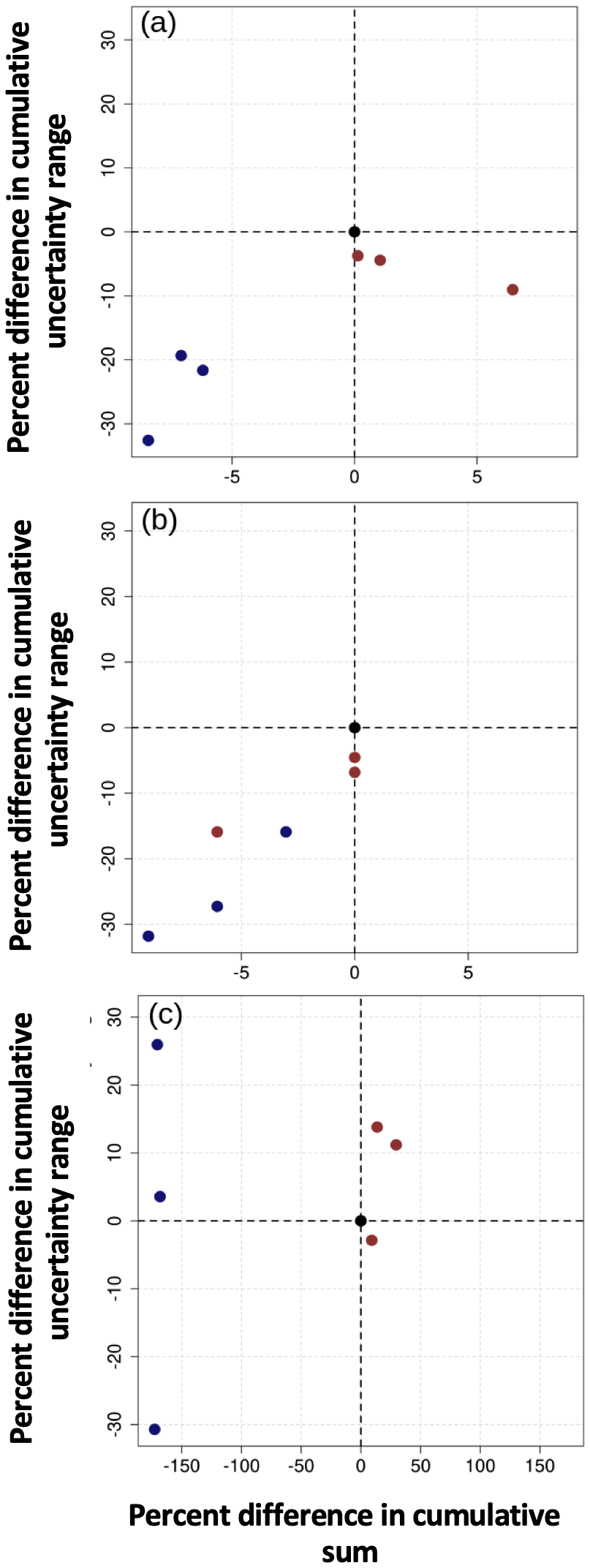
Figure 5 Comparison of percent differences from cumulative sums and associated uncertainty (95 %  CI) between greenhouse gas fluxes derived from automated measurements (F_A) and using an optimized sampling approach (tuLHs) or a fixed temporal stratification. Differences are represented for soil CO₂ (a), soil CH₄ (b), and soil N₂O (c) fluxes. The black circle in the center (0, 0) of a plot represents the values derived from automated measurements (F_A). Blue circles represent estimates from fixed temporal stratification, and red circles represent estimates from an optimized sampling approach (tuLHs). Estimates were calculated based on the 258 available automated measurements (Fig. 2), and numeric estimates are in Table S3. Note the difference in the scale of the x axis among panels.

The FTS underestimated the cumulative flux (−9.1 %, −6.1 %, −3.1 %) and the uncertainty (−31.8 %, −27.3 %, −15.9 %) of F_ACH₄ for k = 12, 24, and 48, respectively (Fig. 5b). In contrast, the tuLHs approach underestimated the cumulative flux (−6.1 %) only for k = 12 but slightly underestimated the uncertainty (−15.9 %, −6.8 %, −4.5 %) for k = 12, 24, and 48, respectively (Fig. 5b).

The FTS substantially underestimated the cumulative flux (−168 %, −170 %, −173 %) of F_AN₂O for k = 12, 24, and 48, respectively. Uncertainty was overestimated for k = 12 and 24 (3.6 % and 26 %) and underestimated for k = 48 (−31 %; Fig. 5c). In contrast, the tuLHs approach overestimated the cumulative flux less (29.5 %, 13.4 %, 9.1 %) for k = 12, 24, and 48, respectively (Fig. 5c). This approach underestimated the uncertainty for k = 12 (−11.2 %) and k = 24 (−13.8 %) but overestimated the uncertainty by 2.9 % for k = 48 (Fig. 5c). These results show that the tuLHs approach consistently provided closer estimates for cumulative sums and uncertainty ranges than an FTS for all GHG fluxes.

4 Discussion

Applied challenges, such as quantifying the role of soils in nature-based solutions, require accurate estimates of GHG fluxes. To do this, two fundamental problems exist for designing environmental monitoring protocols: where and when to measure. Ultimately a monitoring protocol aims to quantify the attributes of an ecosystem so that it can be compared in time within that ecosystem or with other ecosystems. Because we cannot measure everything, everywhere, and all the time, we can argue that any monitoring protocol has assumptions based on physical, economic, social, and practical reasons to address a specific scientific question. These assumptions for designing monitoring protocols could result in misleading, biased, or wrong conclusions, and therefore it is critical to assess the consequences of different monitoring efforts. As Hutchinson (1953) described in “The Concept of Pattern in Ecology”, we do not always know if a given pattern is extraordinary or a simple expression of something which we may learn to expect all the time.

Automated measurements have revolutionized our understanding of the temporal patterns and magnitudes of soil GHG fluxes (Savage et al., 2014; Bond-Lamberty et al., 2020; Tang et al., 2006; Capooci and Vargas, 2022b). These measurements have limitations in representing spatial variability and have higher equipment costs that limit their broad applicability across study sites (Vargas et al., 2011). Consequently, discrete manual measurements are a common approach to simultaneously measure multiple GHG fluxes and report patterns, budgets, and information to parameterize empirical and process-based models (Phillips et al., 2017; Wang and Chen, 2012). In this study, we argue that the convenience of simultaneously measuring multiple GHGs using FTS may result in biased estimates. Therefore, optimization of sampling protocols is needed to provide insights to improve measurement protocols when there is a limited number of measurements in time (i.e., k = 12, 24, 48).

We show that the magnitude of one GHG flux is not associated with a linear increase or decrease in another GHG flux, and the temporal dependencies of each GHG flux are different (Fig. S1). Therefore, it is not possible to infer the dynamics of one GHG flux based solely on information from another under the assumption that they share similar (or autocorrelated) biophysical drivers. These results imply that the magnitudes and temporal patterns of GHGs are different and therefore do not support an FTS approach for simultaneous measurements of GHG fluxes from soils.

Multiple studies have shown that the relevance of different biophysical drivers (e.g., temperature, moisture, light) is different for soil CO₂, CH₄, or N₂O fluxes (Luo et al., 2013; Tang et al., 2006; Ojanen et al., 2010). Our results show that soil CO₂ fluxes have a strong temporal dependence (Fig. S2a), likely due to the strong relationship between these fluxes and soil temperature in this and other temperate mesic ecosystems (Hill et al., 2021; Bahn et al., 2010; Barba et al., 2019). The temporal dependence decreased for soil CH₄ fluxes (Fig. S2b), where there is less evidence for such a strong correlation with soil temperature in this and other temperate mesic ecosystems (Bowden et al., 1998; Castro et al., 1995; Warner et al., 2019; Barba et al., 2019). It has been reported that multiple variables and complex relationships are usually needed to explain the variability in soil CH₄ fluxes in forest soils, as there is a delicate balance between methanogenesis and methanotrophy (Luo et al., 2013; Castro et al., 1994; Murguia-Flores et al., 2018). In contrast, soil N₂O fluxes had no temporal dependence (Fig. S2c), showing decoupling from the observed patterns of soil CO₂ and CH₄ fluxes (Wu et al., 2010), likely as a result of independent biophysical drivers regulating soil N₂O fluxes (Luo et al., 2013; Bowden et al., 1993; Ullah and Moore, 2011).

To address the limitations of an FTS protocol, we propose a novel optimization approach (i.e., tuLHs) to reproduce the probability distribution and the temporal dependence of each original time series of GHG fluxes. Traditional methods usually optimize subsamples by either individually focusing on reproducing the probability distribution of the original information (Huntington and Lyrintzis, 1998) or reproducing the temporal dependence of the original information (Gunawardana et al., 2011). The tuLHs is a simple approach that uses the univariate probability distribution function and the temporal correlation function (i.e., variogram) as objective functions for each GHG flux. Our results show that optimized subsamples do not coincide in time for the three GHGs, suggesting that information should be collected based on each GHG flux's specific statistical and temporal characteristics (Fig. 1). This study provides a proof of concept for the application of the tuLHs. It demonstrates how an optimization approach provides insights to design monitoring protocols and improve soil GHG flux estimates.

The more temporal data we can collect, the better, but in many cases, measurement protocols are limited to a few measurements per year (i.e., k = 12 to 48). Our results demonstrate that for a small sample size (i.e., k = 12), the optimized measurements for soil CO₂ fluxes are consistently spread across the year, and for soil CH₄ fluxes are centered within the growing season because of their strong temporal dependence. For the case of soil N₂O fluxes, the variogram shows a constant temporal variability, meaning there is no temporal dependence. Therefore, the optimized measurements are concentrated within the fall season due to their distribution probability (Fig. 1a). Our optimization approach shows how measurements can be distributed across time as more samples are available (i.e., k = 24 to 48; Fig. 1b and c) and demonstrates that optimization is critical when a limited number of measurements are available. In other words, a few measurements properly distributed across time provide better agreement with information derived from automated measurements. A similar conclusion was proposed for the spatial distribution of environmental observatory networks, where a network of a few sites properly distributed (e.g., across a country) improves our understanding of the target variable more than a spatially biased network (Villarreal et al., 2019). Thus, a representativeness assessment of information collected across time and space is needed to evaluate environmental measurements and quantify nature-based solutions accurately.

We highlight that this optimization approach should be implemented across different ecosystems as it will result in site-specific recommendations. The tuLHs can be applied to any time series length and with any time step (e.g., hours, days), but specific results will be representative of the probability distribution and the temporal dependence of the selected time series. What is essential is to question if a few measurements from an experiment represent the reality of the physical world because if limited information is available, then the actual probability distribution and temporal dependence of the phenomena could be an unknown unknown. In other words, with few measurements, we may not be aware of and we will not be able to know which is the actual probability distribution and temporal dependence of the studied phenomena. To address this challenge, we tested the tuLHs approach with high-temporal-frequency information representing the probability distribution of multiple soil GHG fluxes at the daily time step across a calendar year.

In this case study, the year chosen had typical climatological conditions, and we demonstrated that the statistical properties of the different GHG fluxes differ. Consequently, this study questions the application of the FTS approach to measuring multiple GHGs simultaneously with a limited number of sampling dates (mainly once a month). We recognize that longer time series (e.g., multi-year) could provide more robust optimizations that can be applied to monitoring efforts. We recommend co-locating automated measurements with manual survey efforts to adequately capture the temporal and spatial variability in soil GHG fluxes at study sites.

There are several implications of biased monitoring protocols for understanding soil GHG fluxes and nature-based solutions. First, temporal patterns and temporal dependency may need to be revisited for studies using an FTS approach. Soil GHG fluxes have complex temporal dynamics that vary from diurnal to seasonal and annual scales (Vargas et al., 2010) that a few measurements following an FTS approach cannot reproduce (Barba et al., 2019; Bréchet et al., 2021). Second, soil GHG fluxes could present hot moments, which are transient events with disproportionately high values that are often missed with an FTS approach (Vargas et al., 2018; Butterbach-Bahl et al., 2004). Third, cumulative sums and uncertainty ranges are biased or misleading when derived using an FTS approach (Tallec et al., 2019; Lucas-Moffat et al., 2018; Capooci and Vargas, 2022b). Our study demonstrates that an optimized approach consistently provided closer estimates for cumulative sums and uncertainty ranges when compared with automated measurements (Fig. 5). We postulate that representing the variability in soil N₂O fluxes is more sensitive to the FTS approach (> 170 % and  > 30 % for cumulative sums and uncertainty ranges, respectively) than for soil CH₄ and CO₂ fluxes. Fourth, it is possible that if the information derived from an FTS approach is biased, then functional relationships could also be different from those derived from automated measurements (Capooci and Vargas, 2022a). It has been argued that hypothesis testing and our capability of forecasting responses of soil GHG fluxes to changing climate conditions is also biased with information from the FTS approach (Vicca et al., 2014). Finally, because soils have a central role in nature-based solutions within countries and across the world (Griscom et al., 2017; Bossio et al., 2020), accurate measurements are required to assess management practices, environmental variability, and the contribution of GHGs from soils.

5 Conclusion

We highlight that we only sometimes know if a given pattern is extraordinary or a simple expression of something which we may learn to expect all the time. Arguably, there is bias in our understanding of the probability distribution and temporal dependency of soil GHG fluxes across the world because most results are based on a few manual measurements (e.g., once a month) following an FTS approach. Currently, it is unknown how large such bias could be across studies and ecosystems, but because most studies lack high-temporal-frequency information, the real probability distribution and temporal dependency of soil GHG fluxes may remain unknown in most study sites. What is essential is to question if the observed patterns, derived from an FTS approach, are enough for improving our understanding of soil processes or are results that we have learned to expect.

We postulate that with emergent technologies, there is convenience in measuring multiple GHGs from soils; however, few measurements collected at fixed time intervals result in biased estimates. We recognize that potential measurement bias depends on each GHG flux's magnitudes and temporal patterns and could be site-specific. Nevertheless, evaluations are needed to quantify potential bias in estimates of GHG budgets and information used for model parameterization and environmental assessments. Furthermore, the underlying assumption that each GHG flux responds similarly to biophysical drivers may need to be tested across multiple ecosystems to quantify how few measurements influence our understanding of magnitudes and temporal patterns of soil GHG fluxes.

In this study, we present a proof of concept and propose a novel approach (i.e., temporal univariate Latin hypercube sampling) that can be applied with site-specific information on different ecosystems to improve monitoring efforts and reduce the bias in GHG flux measurements across time. We highlight that constant biased environmental monitoring may provide confirmatory information, which we have learned to expect, but modifications of monitoring protocols could shed light on new or unexpected patterns. These new patterns are the ones that will test paradigms and push science frontiers.