Satellite data reveal earlier and stronger phytoplankton blooms over fronts in the Gulf Stream region

Fronts affect phytoplankton growth and phenology by locally reducing stratification and increasing nutrient supplies. Biomass peaks at fronts have been observed in situ and linked to local nutrient upwelling and/or lateral transport, while reduced stratification over fronts has been shown to induce earlier blooms in numerical models. Satellite imagery offers the opportunity to quantify these induced changes in phytoplankton over a large number of fronts and at synoptic scales. Here we used 20 years of sea surface temperature (SST) and chlorophyll a (Chl a) satellite data in a large region surrounding the Gulf Stream to quantify the impact of fronts on surface Chl a (used as a proxy for phytoplankton) in three contrasting bioregions, from oligotrophic to blooming ones, and throughout the year. We computed an heterogeneity index (HI) from SST to detect fronts and used it to sort fronts into weak and strong ones based on HI thresholds. We observed that the location of strong fronts corresponded to the persistent western boundary current fronts and weak fronts to more ephemeral submesoscale fronts. We compared Chl a distributions over strong fronts, over weak fronts, and outside of fronts in the three bioregions. We assessed three metrics: the Chl a excess over fronts at the local scale of fronts, the surplus in Chl a induced at the bioregional scale, and the lag in spring bloom onset over fronts. We found that weak fronts are associated with a local Chl a excess weaker than strong fronts, but because they are also more frequent, they contribute equally to the regional Chl a surplus. We also found that the local excess of Chl a was 2 to 3 times larger in the bioregion with a spring bloom than in the oligotrophic bioregion, which can be partly explained by the transport of nutrients by the Gulf Stream. We found strong seasonal variations in the amplitude of the Chl a excess over fronts, and we show periods of Chl a deficit over fronts north of 45^∘ N that we attribute to subduction. Finally we provide observational evidence that blooms start earlier over fronts by 1 to 2 weeks. Our results suggest that the spectacular impact of fronts at the local scale of fronts (up to +60 %) is more limited when considered at the regional scale of bioregions (less than +5 %) but may nevertheless have implications for the region's overall ecosystem.

1 Introduction

Phytoplankton form the basis of marine food webs and are key players in the ocean carbon cycle. The transport of limiting nutrients to the sunlit euphotic layer by advective and convective processes and the amount of light received by the cells – which is closely related to the stratification of the water column – are two important factors that control their growth. As there are marked contrasts in nutrient and light availability in the ocean, it follows that the global ocean can be divided into different regional biomes (or bioregions), characterized by different phytoplankton abundances and seasonality (Longhurst, 2007; Vichi et al., 2011; Bock et al., 2022). The contrasts between biomes are largely explained by consistent physical forcings and environmental conditions (such as nutrient sources), operating at the biome scale, which determine how the two main controlling factors, nutrient and light, limit growth. For example, subtropical gyres are areas where negative wind stress curl induces a deepening of the thermocline and nutricline, resulting in oligotrophic biomes where productivity is relatively constant and low throughout the year. At higher latitudes, where the wind stress curl is positive, the nutricline is shallower; the strong seasonality of the vertical mixing will induce a multi-stage operation, with a time of reduced productivity and convective nutrient supply in winter when the mixing is strong, as well as a bloom in spring when the stratification sets in (Wilson, 2005; Williams and Follows, 2011). In addition to these large-scale patterns, there has been considerable evidence over past years that the nutrient and light environments are modified at ocean fronts, with consequences for phytoplankton (see reviews by Lévy et al., 2012; Mahadevan, 2016; Lévy et al., 2018).

Ocean fronts are narrow zones where horizontal gradients in water properties (temperature, salinity, nutrients, etc.) are significant (Belkin et al., 2009) and are sometimes described as discontinuities because of their abrupt nature (Mauzole, 2022). Lévy et al. (2018) distinguished two types of fronts. Persistent fronts like those associated with the Gulf Stream and Kuroshio are locked in place by the coastal boundary and large-scale atmospheric forcing. Their forcing is directly balanced by submesoscale symmetric instability, which takes energy mostly from the kinetic energy of the jet, and baroclinic instability, which converts the potential energy of the sloping density surfaces into large meanders and eddies. Their ephemeral cousins are continuously forming, moving, and dissipating at the ocean surface. They are being strained by mesoscale eddies, which intensifies their geostrophic along-front currents and feeds fluid instabilities, generating submesoscale vortices and filaments. Importantly, a front will generate a cross-frontal ageostrophic secondary circulation – an overturning circulation which tries to flatten the density surfaces in the front, with upwelling on the warm side of the front and downwelling on the cold side (Thomas et al., 2008; McWilliams, 2016; Mahadevan et al., 2020). The highly energetic persistent fronts are characterized by a deep vertical velocity structure that reaches the thermocline, while ephemeral fronts have associated cross-frontal secondary circulations that are generally confined to the vertically well-mixed upper layer of the ocean. Frontal dynamics also involves increased stratification, reduction in mixed-layer depth, and suppression of vertical mixing at the front (Thomas and Ferrari, 2008).

Fronts may affect phytoplankton in various ways. The upward branch of the secondary circulation may enhance phytoplankton growth by transporting nutrients into the euphotic zone (Johnson et al., 2010; Wilson, 2021). The downward branch may subduct biomass and excess nutrients into the subsurface (Calil et al., 2011; Omand et al., 2015; Hauschildt et al., 2021). Persistent fronts may act as a conduit for nutrients over large distances, known as nutrient streams (Pelegrí et al., 1996; Williams et al., 2011; Long et al., 2022). Advective transport along fronts may transport nutrients to the shallow flanks of subtropical gyres (Letscher et al., 2016; Gupta et al., 2022). Finally, in highly seasonal regimes where productivity is slowed in winter due to deep mixing, increased restratification over fronts may promote localized phytoplankton blooms before the large-scale outburst associated with seasonal stratification (Mahadevan et al., 2012). These effects all together are responsible for local anomalies in the distribution of phytoplankton over fronts. Thus fronts not only are a physical boundary but also constitute specific habitats for phytoplankton (Mangolte et al., 2023).

Despite numerous local observations and a strong theoretical basis for the physical processes affecting phytoplankton growth over fronts (e.g., recent studies by Marrec et al., 2018; Little et al., 2018; de Verneil et al., 2019; Ruiz et al., 2019; Uchida et al., 2020; Kessouri et al., 2020; Tzortzis et al., 2021), their integrated contribution at the scale of regional biomes is still largely unknown. Ephemeral fronts move and dissipate continuously on timescales of days to weeks and are thus particularly difficult to sample. This limitation is reinforced by the fact that only a limited number of fronts can be observed with in situ field observations. Thus satellite-derived estimates of chlorophyll a (hereafter Chl a), although limited to the surface of the ocean and an imperfect proxy for phytoplankton biomass, are the only data that allow the impact of fronts to be tracked synoptically over large areas. A first attempt to assess the contribution of small-scale physical processes to regional satellite Chl a budgets was based on a geostatistical analysis derived from data at 9 km resolution (Doney et al., 2003), extended later in Glover et al. (2018), with which they examined the change in spatial variance with distance. This methodology was too coarse to reveal the impact of frontal processes but confirmed the important role of mesoscale eddies in stirring large-scale gradients of phytoplankton abundance. The role of fronts has been assessed with three different methods. Guo et al. (2019) combined ocean color data with altimetry and drifting floats, and they estimated that, over subtropical gyres of the global ocean, the respective contributions of mesoscale dynamics and submesoscale frontal dynamics to high-Chl a anomalies were comparable in magnitude. Keerthi et al. (2022) proposed an approach based on the deconvolution of local Chl a time series into different timescales; they observed that subseasonal timescales contributed roughly 30 % of the total satellite Chl a variance and were associated with small (<100 km) spatial scales – which included both the mesoscale and the submesoscale. Finally, the most quantitative approach, and the only one directly related to co-localization with fronts, was proposed by Liu and Levine (2016), which they applied to the North Pacific subtropical gyre. They detected sea surface temperature (SST) fronts by computing an index that measures the local heterogeneity of the SST field from satellite data. This allowed them to compare satellite Chl a values over areas impacted by fronts (characterized by a large value of the heterogeneity index) with values over areas that were not impacted. They found that the increase in Chl a over the fronts was negligible in summer but reached almost 40 % in winter.

Here we build on this last approach and quantify the surplus Chl a induced by fronts at the scale of biomes. The excess Chl a over fronts depends on how efficient fronts are at supplying nutrients, which itself depends on how deep the fronts reach into the nutricline, on the seasonality of this vertical supply, and also on the presence of nutrient sources that are advected horizontally along the front. The impact of fronts is also expected to differ between biomes, with submesoscale advection of nutrients likely to be more important in oligotrophic biomes where other nutrient supply routes are scarce, as well as submesoscale restratification in blooming biomes. Finally, the regional surplus Chl a induced by fronts at the scale of biomes will depend on the spatiotemporal footprint of fronts, which also varies seasonally (Callies et al., 2015) and regionally (Mauzole, 2022). Thus, our intention is to explore and quantify how the contribution of fronts to biome-scale Chl a varies in three contrasted biomes, ranging from subtropical to subpolar; varies throughout the year; and varies with the occurrence and strength of fronts.

We focus our analysis on the North Atlantic region surrounding the Gulf Stream, where multiple biomes and fronts of different strengths are found in a limited geographical area (Bock et al., 2022) with strong seasonality. In the south, our study area encompasses part of the North Atlantic subtropical gyre, characterized by an oligotrophic regime and year-long low productivity. In the north, north of the Gulf Stream jet, is a more productive subpolar regime characterized by a recurrent spring bloom. In between, there is a moderately productive regime, with maximum productivity in winter. Another feature that makes this study area particularly relevant is that it has two strong persistent fronts, the Gulf Stream and the shelf-break front, which are both associated with strong and deep-reaching vertical circulations (Flagg et al., 2006; Liao et al., 2022), with the Gulf Stream being a recognized horizontal nutrient pathway toward the North Atlantic (Pelegrí et al., 1996; Williams and Follows, 2011). But there are also a plethora of ephemeral fronts continuously forming at more random locations (Drushka et al., 2019; Sanchez-Rios et al., 2020).

2 Methods and data

We use satellite data of Chl a and SST and build on the approach of Liu and Levine (2016) to distinguish between persistent and ephemeral fronts. We evaluate the impact of both types of fronts on Chl a on the basis of three indicators: the excess (or deficit) Chl a over fronts at the local scale of the front, the surplus Chl a attributable to fronts at the scale of regional biomes, and the change in the timing of the Chl a spring bloom over fronts.

2.1 Data

Our approach combines daily satellite SST data, which are used to detect fronts and sort them by their strength, with daily satellite surface Chl a, from which we derive anomalies over fronts. For Chl a, we used the L3 product distributed by ACRI-ST over the period 2000–2020, generated by Copernicus-GlobColour¹, constructed with data from different sensors (SeaWIFS, MODIS Aqua and Terra, MERIS, VIIRS-SNPP and JPSS1, and OLCI-S3A and S3B), merged and reprocessed, and available daily at 4 km resolution (Garnesson et al., 2019, 2021).

For SST, we used the European Space Agency Sea Surface Temperature Climate Change Initiative analysis product version 2.1 (Merchant et al., 2019; Good et al., 2020a, b), also available daily at 4 km resolution over the period 2000–2020. This product combines data from all available infrared sensors ((A)ATSR, SLSTR, and AVHRR sensors), ensuring good resolution where data are available, unlike other SST products which also include microwave and in situ measurements, resulting in considerable smoothing of the SST field. Where SST data are not available, spatial interpolation is performed to obtain a cloud-free product which, at the cost of resolution of the finer features, provides complete synoptic coverage of our large study area. This interpolation tends to underestimate the detection of fronts, as the SST field is smoother over cloud-covered areas (Merchant et al., 2019). However, the combination of several sensors allows these areas to be reduced to a minimum. Furthermore, we have only considered cloud-free pixels for our analysis, which ensures that cloudy areas are not taken into account in our quantification.

2.2 Delimitation of biomes

Our region of interest is the North Atlantic from 15 to 55^∘ N and from 40^∘ W to the North American shelf break (Fig. 1). We focus on the open ocean and exclude the continental shelf; thus all pixels where water depth is less than 1500 m (red isobath in Fig. 1) are masked. The region is characterized by the presence of a large-scale north–south gradient in Chl a and is sorted into three open-ocean biomes.

The oligotrophic permanent subtropical biome (PSB) – also known as the subtropical gyre permanently stratified biome (Sarmiento et al., 2004) – to the south of our study area is characterized by warm waters and low Chl a (Fig. 1). There is no clear physical boundary to its northern limit, so we have chosen the latitudinal limit of 32^∘ N to delineate it, which roughly corresponds to the 0.1 mg m⁻³ Chl a iso-contour in annual mean Chl a. There is no persistent front in the PSB.

North of 32^∘ N, the seasonal subtropical biome (SSB) – also known as the subtropical gyre seasonally stratified biome (Sarmiento et al., 2004) and as the permanent deep Chl a maximum biome (Bock et al., 2022) – is also mainly oligotrophic, with intermediate levels of Chl a and temperature, and is characterized by slightly increased productivity in winter. It is bounded to the north by the meanders of the Gulf Stream jet. When the Gulf Stream enters the SSB, it conveys warm, nutrient rich, salty waters poleward along the Florida coast up to Cape Hatteras (35^∘ N), where it separates from the continental shelf and meanders essentially zonally. The north wall of the Gulf Stream, so called because of its steep temperature gradient, marks the sharp, sinuous, and unsteady northern limit of the SSB.

To the north of the Gulf Stream is the Slope Sea which extends to the shelf break, with colder and fresher waters (Linder and Gawarkiewicz, 1998). Aligned with the shelf break, a persistent front with an intensified surface jet separates the shelf waters (excluded from this study) from the Slope Sea. This highly productive subpolar biome (PB) – also known as subpolar waters (Sarmiento et al., 2004) and as high-chlorophyll bloom (Bock et al., 2022) – is characterized by a strong spring bloom whose onset is tied to the spring stratification of the mixed layer. The shelf-break front is thus comprised within the PB.

The position of the north wall of the Gulf Stream, which delimits the SSB and the PB (black meandering contour in Fig. 1a–b), is determined at each daily time step by thresholding the daily SST map. The daily threshold values (black vertical line in Fig. 1c) are determined from the daily SST distributions above 32^∘ N (blue line, continued by the yellow line in Fig. 1c). Indeed, the Gulf Stream is easily identifiable in this distribution as it is manifested by a temperature peak (yellow line in Fig. 1c). To detect the start of this peak, which marks our boundary, we fit the peak with a Gaussian and define the threshold temperature as the mean minus twice the standard deviation. Then, the threshold temperature time series is median filtered over an 8 d window to eliminate spurious detection anomalies. This separation method ensures quasi-unimodal Chl a distributions within each biome (Fig. 1d).

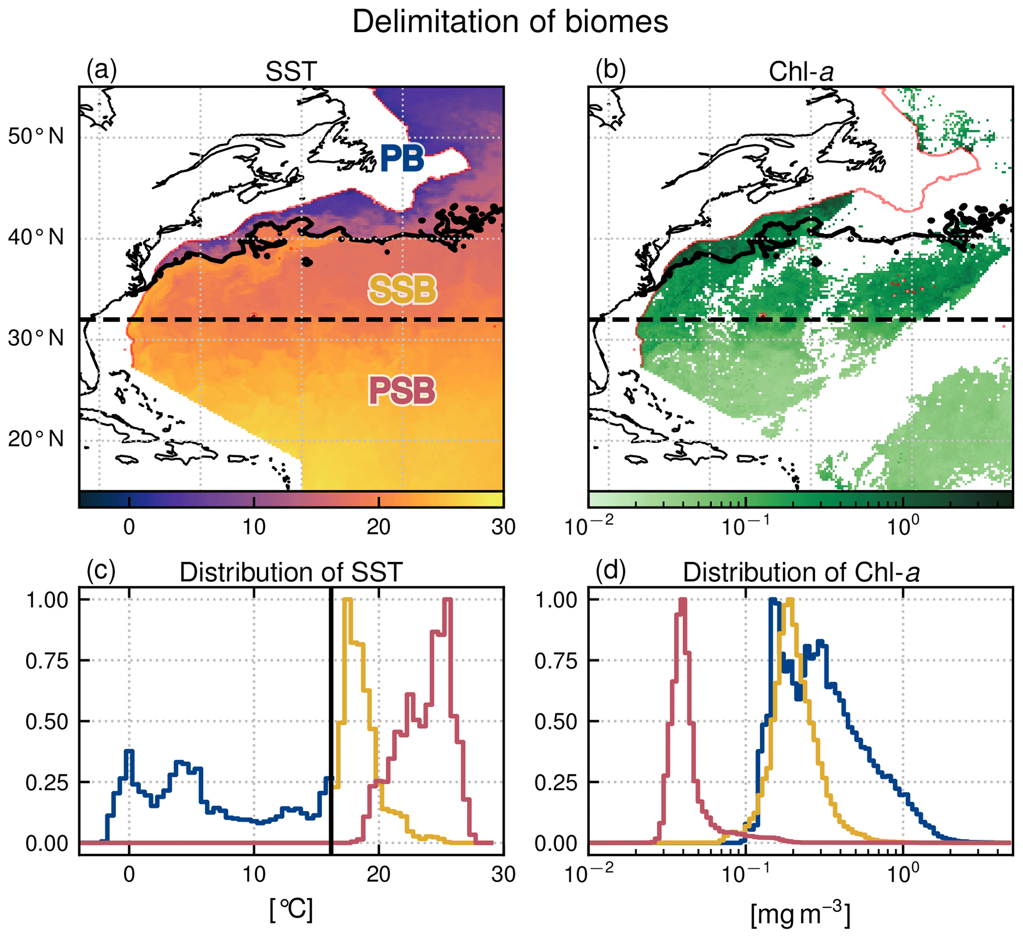
Figure 1 Delimitation of the three biomes in the open-ocean Gulf Stream extension region: the permanent subtropical biome (PSB, south of the dashed line at 32^∘ N), the seasonal subtropical biome (SSB, between 32^∘ N and the meandering Gulf Stream northern wall on that day marked with the black contour), and the subpolar biome (PB, north of the Gulf Stream northern wall). (a) SST and (b) Chl a snapshots on 22 April 2007 (with data masked by clouds in white). The red line follows the 1500 m isobath. Data on the continental shelf (<1500 m) are not considered here and have been masked. (c) SST and (d) Chl a distribution within each biome for the same day (PB: blue; SSB: yellow; PSB: red). The black line in panel (c) shows the SST threshold value detected to delimit the Gulf Stream northern wall (see Sect. 2.2).

2.3 Front detection

Our front detection method aims to sort the domain into pixels that are located (or not) over fronts at each daily time step. We follow the approach of Liu and Levine (2016) that builds upon the well established Cayula–Cornillon algorithm (Cayula and Cornillon, 1992; Belkin and O'Reilly, 2009) and identify pixels as belonging to fronts when the region in the vicinity of the pixel is characterized by high SST heterogeneity. More precisely, on each pixel and for each time step, we compute an heterogeneity index (HI) which quantifies the heterogeneity of the SST in a square window comprising a few pixels (7×7) centered on the pixel of interest. Thus HI measures the SST heterogeneity at spatial scales less than 30 km. This spatial scale captures the heterogeneity associated with submesoscale fronts and persistent fronts (which are wider than submesoscale fronts), with the edges of mesoscale eddies (which are also considered as fronts) but not with the center of eddies as their diameter is generally >100 km (see, for instance, Contreras et al., 2023, which nicely shows the scales of these different features in this region). The HI is defined as the weighted sum of the skewness γ, standard deviation σ, and bimodality B of SST within the window ($\text{HI}=a\left(b\mathit{\gamma }+c\mathit{\sigma }+dB\right)$, with a, b, c, and d constant normalization coefficients).

We computed the bimodality as the L2 norm of the difference between the SST histogram (with bins of 0.1 ^∘C) and a Gaussian fit of the histogram. We chose this method because it was simpler to implement and more robust than that of Liu and Levine (2016) which computed the normalized absolute difference between a polynomial fit of order 5 of the SST histogram and a Gaussian fit of the histogram, the polynomial fit often being poorly constrained. We normalized each component by its variance (b, c, and d being defined as the inverse of the standard deviation of each component computed over 1 year), as opposed to Liu and Levine (2016), who normalized the coefficients by their annual maximum. This avoided putting too much weight on extrema. Finally we normalized HI (coefficient a) such that 95 % of values are below an arbitrary value of 9.5. For simplicity, the normalization coefficients were computed for the year 2007 and used over the entire time series. An example of the resulting HI over a single front is given in Fig. 2; elevated HI values are located along the curved SST gradient to the northeast of the window. We performed sensitivity tests on the different parameters used to compute HI, namely the number of pixels in the rolling window and the choice of normalization coefficients. Our results are weakly sensitive to the choice of these parameters (Fig. A1).

At each time step, we sorted the pixels into those belonging to strong fronts (defined as HI>10), those belonging to weak fronts (defined as $\mathrm{5}<\text{HI}<\mathrm{10}$), and those that do not belong to fronts (when HI<5, called “background” in the following). Sorting fronts by range of HI enabled us to roughly separate the persistent fronts, which are associated with the strongest SST gradients (strong fronts), from the ephemeral fronts, associated with weaker gradients (weak fronts). The choice of the two HI thresholds is somewhat arbitrary, but it is supported by the HI distributions presented below.

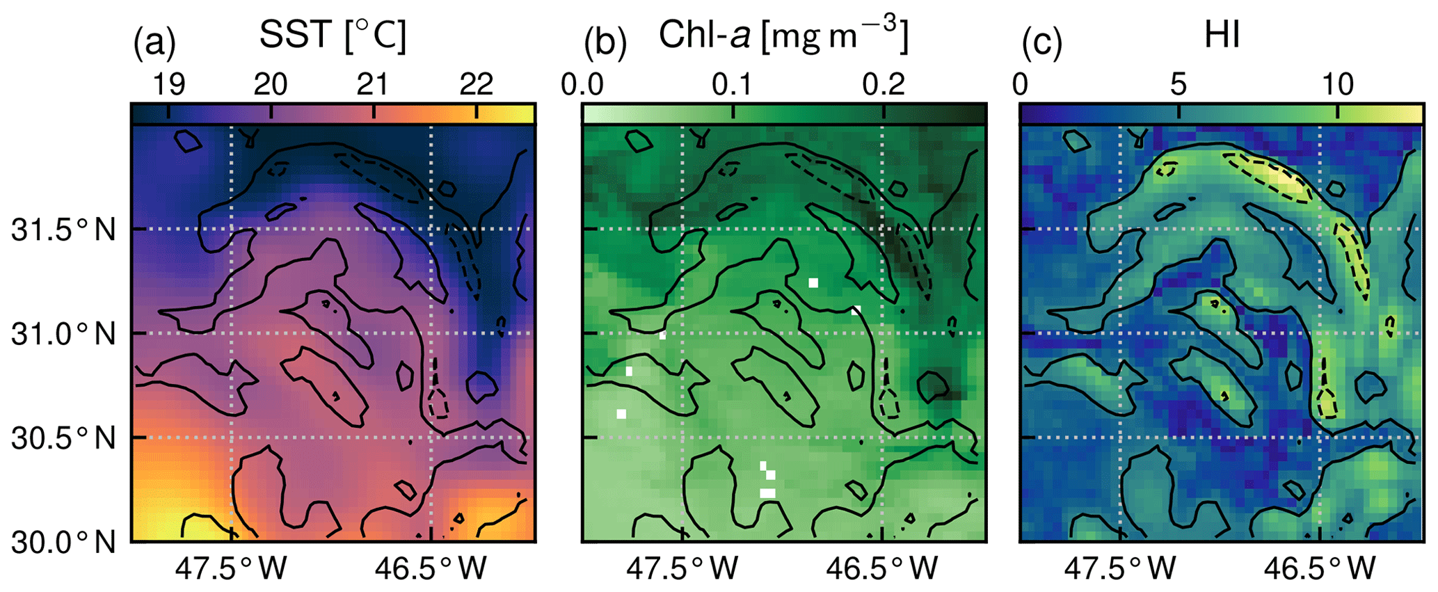
Figure 2 The SST, Chl a, and heterogeneity index (HI) of a front on 7 July 2007. The plain and dashed contours correspond to HI values of 5 and 10. This front is categorized as weak. Chl a are elevated inside the front.

2.4 Quantification of the impact of fronts on Chl a

In order to quantify how Chl a is affected by fronts at the local scale of fronts, we compared the distributions of Chl a over fronts and the distributions of Chl a outside of fronts. Distributions were computed over 8 d windows to limit the influence of particularly cloudy days. They were computed within each biome, and over latitudinal bands of width 5^∘, to minimize the influence of the large-scale north–south gradient in Chl a. Distributions were compared in terms of their median value, but using mean values yielded similar results (see Fig. A2 for seasonal distributions and their medians over and outside of fronts within the three biomes). We defined and computed the local excess Chl a, E (expressed in percent), as the median value over fronts minus the median value in the background, divided by the median value in the background, for each distribution. We repeated this for weak and strong fronts.

To quantify the large-scale impact of fronts on Chl a at the scale of biomes, we computed the biome surplus of Chl a (S) which we defined and computed as the relative difference (expressed in percent) between the mean Chl a over the entire biome (MT) and the mean Chl a over the background (MB): $S=(\text{MT}-\text{MB})/\text{MB}$. Thus the surplus S measures the extra quantity of Chl a at the scale of the biome (MT−MB), relative to what would be the situation in the absence of fronts (MB), and thus accounts for the local excess over fronts (E) but also for the proportion of fronts in a given biome. To better understand the meaning of the surplus, let us consider the simplified case where Chl a is homogeneously doubled over fronts compared to the background value, i.e., when E=100 %; in that case, the surplus Chl a is 50 % if there are 50 % of fronts and is 1 % if there are 1 % of fronts. Note that the computation of the local excess E is based on median values because it relies on the comparison of distributions, while for the computation of the biome surplus S, we used mean values in order to be conservative.

Finally, the subpolar biome is characterized by a spring bloom, of which we measured the onset date both over fronts and in the background, for each year. We defined the lag in bloom onset L as the bloom onset day over fronts minus the bloom onset day in the background. Because the spring bloom onsets propagate from south to north, bloom onset days were inferred over latitudinal bands of limited width (5^∘). We pooled apart front and non-front pixels and computed the onset dates and their uncertainty based on the time series of the fronts and non-front Chl a median value. We first filtered the Chl a median time series with a low-pass Butterworth filter of order 2 and cutting frequency $\mathrm{1}/\mathrm{20}$ d⁻¹. The filtered time series displayed strong variations in their phenology from year to year, but a bloom was always discernible. We considered data from February to July, which allowed us to isolate the spring bloom and exclude the fall bloom. We detected the maximum value of Chl a in this time window and defined the bloom onset as the time of maximum Chl a derivative prior to the time of maximum Chl a. We defined the uncertainty in bloom onset date as the standard deviation of all days for which the Chl a derivative is above 90 % of its maximum value. We defined the uncertainty in lag L as the square root of the sum of squared uncertainties in fronts and background. Finally, we estimated the mean lag (over the 20 years of data and for each latitudinal band) as the weighted averaged lag, with the weights equal to the inverse of the uncertainties; and we estimated the mean lag uncertainty as the weighted standard deviation of all lag values around the mean lag, with the weights equal to the inverse of the uncertainties. Our Eulerian approach relies on the hypothesis that the bloom evolves coherently in the background (or over fronts, respectively) within each latitudinal band, which is suggested by high-resolution models of the bloom (e.g., Lévy et al., 2005; Karleskind et al., 2011). It is imperfect as the bloom evolves along Lagrangian trajectories but provided very consistent results.

3 Results

3.1 Distribution of fronts

Our definition of weak fronts and strong fronts is primarily based on thresholds derived from the HI distributions (Fig. 3, dashed red line). In each biome, the majority of HI values are below 5, and as mentioned before, we used this threshold to distinguish pixels in the background from those over fronts (when HI>5). Secondly, the number of points in the HI distribution decreases sharply as the HI value increases above 5, reflecting the fact that fronts with stronger SST gradients are much less frequent than fronts with weaker gradients, as one would expect. We used the HI threshold of 10 to distinguish weak fronts from strong fronts. This separation is imperfect, as seen, for instance, in Fig. 2 where a few pixels with HI values larger than 10 appear at the core of an otherwise weak front.

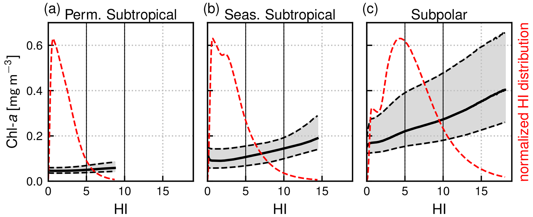
Figure 3 Normalized distribution of the heterogeneity index (HI, dashed red line) within each biome and distribution of Chl a as a function of HI (representing front strength) over the full period of 2000–2020. Shown are the median value of the Chl a distributions (solid black line) and first and third quartiles (dashed lines). Note that 0.5 % of pixels have outstanding large HI values and are not included here.

However, the choice of these two HI thresholds is also guided by the resulting global spatial climatology of weak and strong fronts (Fig. 4). Weak fronts are abundant, and more or less evenly distributed, over a broad band around and north of the Gulf Stream jet (Fig. 4a). To the south of the Gulf Stream jet, weak fronts are less prevalent, with nevertheless more fronts on the edges of the subtropical gyre (around 28^∘ N) than in its center. This distribution of weak fronts is consistent with the predominance of mesoscale variability observed along the Gulf Stream system from satellite altimetry (Zhai et al., 2008), as well as the injection of eddy kinetic energy north of the Gulf Stream jet by the Gulf Stream extension. It is thus consistent with the generation process of ephemeral fronts through mesoscale strain.

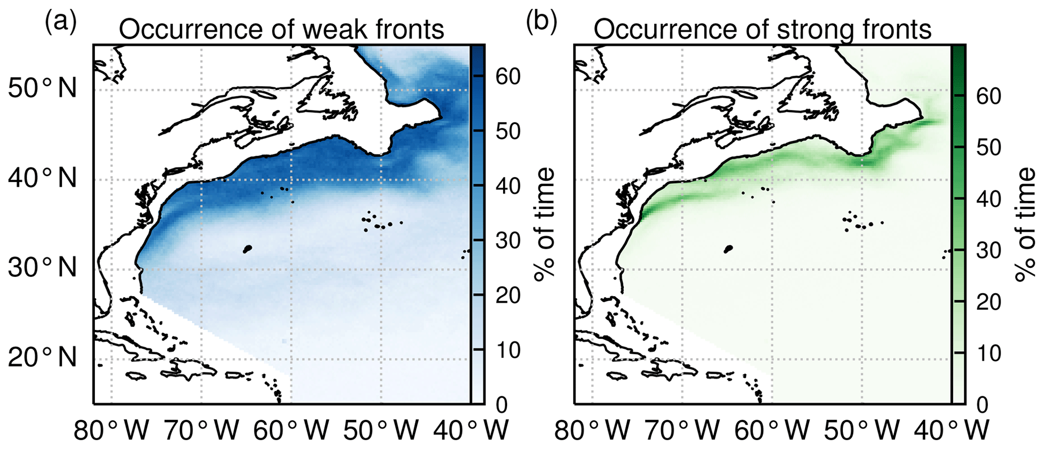
Figure 4 Occurrence of (a) weak fronts and (b) strong fronts expressed as the percentage of time steps over the time series (2000–2020) for which a given pixel is occupied by a front.

The climatological distribution of strong fronts shows that they coincide mainly with the two persistent fronts of the western boundary current system, the Gulf Stream front extending northeast from Cape Hatteras, and the more northerly shelf-break front extending eastward to 50^∘ W, following the northeastern US continental shelf break (Fig. 4b). Thus these contrasted coverages of localized strong fronts and more widespread weak fronts are consistent with the hypothesis that weak fronts capture the ephemeral fronts, whereas strong fronts capture the persistent ones.

With the chosen thresholds, the areal proportion of weak fronts tends to increase from south to north, with 7 %, 19 %, and 42 % of HI values comprised between 5 and 10 in the permanent subtropical, seasonal subtropical, and subpolar biomes, respectively. Regarding strong fronts, they are only present in the seasonal subtropical and subpolar biome, consistent with the fact that the Gulf Stream and shelf-break fronts are located within these biomes, where HI values above 10 account for 6 % and 17 %, respectively.

The fraction of the area occupied by fronts also varies with seasons, with generally fewer fronts in summer (Fig. 5d–f). In the permanent subtropical biome, weak fronts cover on average up to 12 % in spring and drop to 2 % in summer. In the seasonal subtropical biome, the variation is from 27 % to 13 % for weak fronts and 8 % to 4 % for strong fronts. In the subpolar biome, strong fronts cover between 11 % in summer and 26 % at their peak. This seasonality is consistent with other estimates that submesoscale frontal activity is greater in winter due to greater mixed-layer thickness compared to summer (Callies et al., 2015) and also consistent with the most recent modeling results by Dong et al. (2020) in another western boundary current system (the Kuroshio Extension) where they show that the strongest submesoscale dynamics occur with a lag of about a month after the mixed-layer thickness maximum is reached.

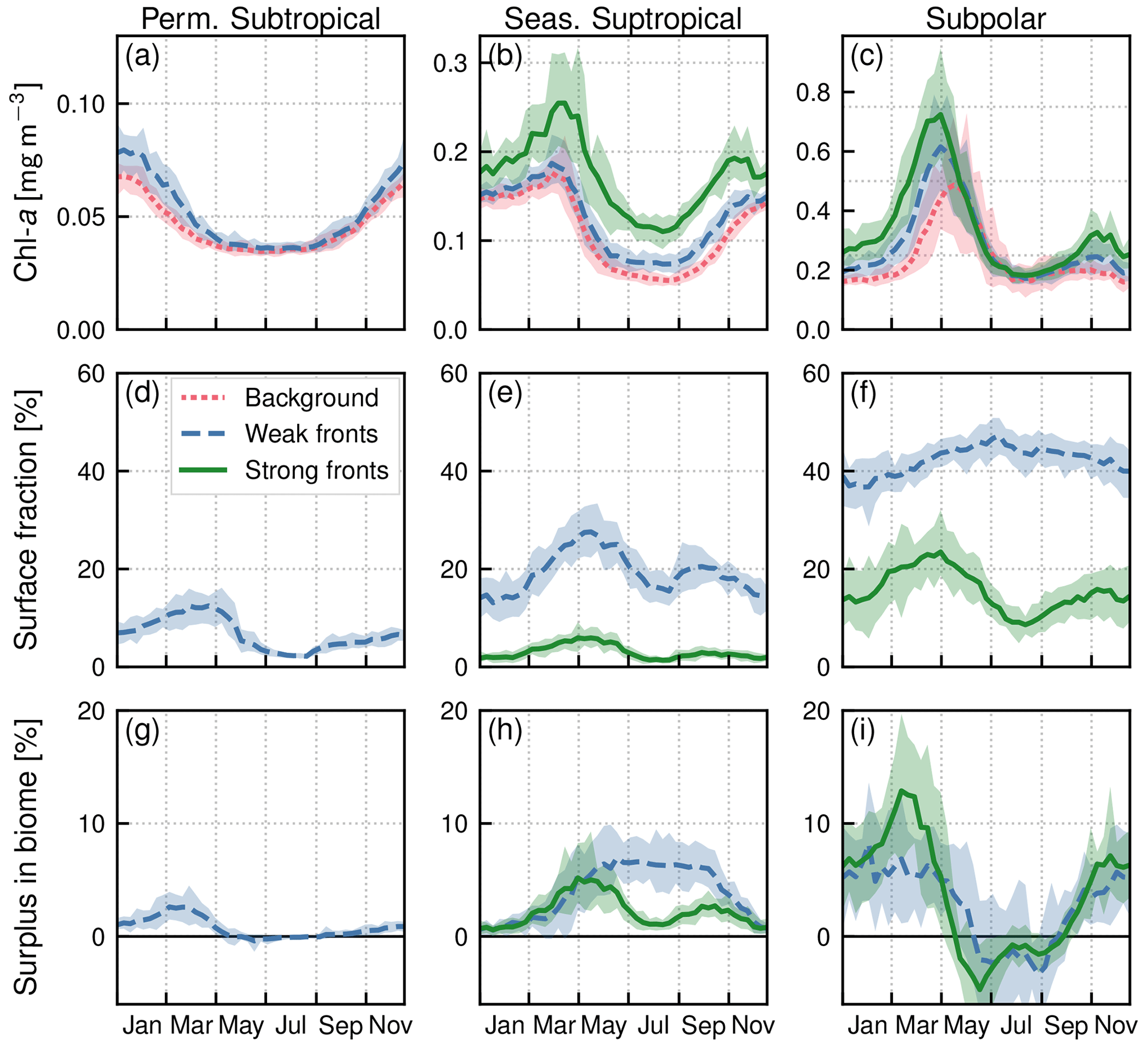
Figure 5 Seasonal climatologies in the permanent subtropical biome (first column), in the seasonal subtropical biome (second column), and in the subpolar biome (third column). (a, b, c) Chl a median values (top row) over weak fronts (blue), strong fronts (green) and background (red). Gaps between the curves represent the local excess over fronts. (d, e, f) Surface fraction occupied by fronts. (g, h, i) Regional Chl a surplus at the scale of the biome. The surplus accounts for the local excess and for the number of fronts (see Sect. 2.4). The plain lines represent the climatological mean, and the envelopes mark the standard deviation over the period 2000–2020. The excess in Chl a is larger over strong fronts than over weak fronts, but weak fronts are more numerous than strong fronts, resulting in a Chl a surplus that can be comparable to or even larger than that in weak fronts.

3.2 Local Chl a excess over fronts

The local Chl a excess over fronts is seen, for example, in Fig. 2, where the highest values of Chl a are found within the HI contour delimiting the front. To quantify this excess over a large number of fronts, we computed for each biome the Chl a distribution sorted by bins of HI (of width 0.1) for the whole time series (Fig. 3). For low values of the heterogeneity index, these distributions are representative of background conditions and reflect the expected differences between biomes: the median Chl a is lowest (0.05 mg m⁻³) in the permanent subtropical biome, intermediate in the seasonal subtropical biome (0.1 mg m⁻³), and highest in the subpolar biome (0.2 mg m⁻³). The Chl a variability throughout the year and within the biome (i.e., the width of the distribution, highlighted by grey shading in Fig. 3) is larger moving northwards because of the higher seasonal variability. Importantly, in all three biomes, Chl a values increase with HI and are also more dispersed as HI increases (Fig. 3). Thus the excess in Chl a depends continuously on the value of HI.

In the permanent subtropical biome (Fig. 5a), the seasonal variations in Chl a are very modest with a weak peak in winter. In the seasonal subtropical biome (Fig. 5b), the seasonal variations are well marked, with a minimum in summer and an increase that starts in fall and peaks in late winter. In the subpolar biome (Fig. 5c), there is a marked bloom in spring with a peak in Chl a in April, followed by an fall bloom albeit with a smaller magnitude. These different phenologies are well documented and largely explained by the differences in the seasonal cycle of the mixed layer, and the relative depths of the winter mixed layer and the nutricline (see, for instance, Lévy et al., 2005, for a description of the drivers of these three production regimes in similar biomes of the northeast Atlantic). In the permanent subtropical biome, the low productivity is due to the fact that winter mixing is not sufficient to provide a substantial convective supply of nutrients; in contrast, in the seasonal subtropical regime, the increase in production in fall starts when the mixed layer deepens and reaches the nutricline, leading to a fall–winter bloom. In the subpolar biome, this fall bloom is interrupted in winter when the mixed layer significantly deepens, diluting phytoplankton cells vertically, and a spring bloom is initiated when the mixed layer stratifies at the end of winter.

In both subtropical biomes, Chl a over fronts is systematically larger than in the background, and this holds throughout the year (Fig. 5a–b). This increase is very modest over the permanent subtropical biome. The local increase over weak fronts also remains modest in the seasonal subtropical gyre but is much larger over strong fronts. Finally in the subpolar biome (Fig. 5c), Chl a is significantly higher over fronts from the fall until the peak of the bloom, but this difference diminishes as the spring bloom decays and throughout summer. We can also note that the standard deviation range of the yearly median values (Fig. 5a–c) is smaller than the differences between fronts and background, which further confirms that these differences are robust over 20 years of data, for the three biomes and the two types of fronts.

Within each biome, the strength of the local excess in Chl a over fronts varies with latitude. In the permanent subtropical biome (Fig. 6), the excess is only detectable north of 25^∘ N and remains modest (E<10 %); it reaches its maximum of 10 % at the beginning and end of the production season. In the seasonal subtropical biome (Fig. 7), the excess is also small in the southern part of the biome (south of 35^∘ N) but strongly increases further north (between 35 and 45^∘ N) and decreases again going even further north (between 40 and 45^∘ N). Moreover, in this biome, the increase is stronger in summer (July–August) compared to winter (December–January). Finally in the subpolar biome, the magnitude of the local excess diminishes going northward. It tends to be stronger during winter and during the bloom and weaker in summer. In fact in summer, the differences are hardly discernible when averaged over the entire biome (Fig. 5c), but there is an excess Chl a in the southern part of the biome (<45^∘ N) and a small deficit in the northern part of the biome (>45^∘ N) (Fig. 8). It ensues that the annual mean local excess in Chl a over fronts has a distinct latitudinal pattern (Fig.9a). The strongest local increase due to fronts is located in the latitudinal band 35–45^∘ N, where the seasonal subtropical and subpolar biomes meet. The excess is 2 to 3 times larger over fronts north of the Gulf Stream (i.e., in the subpolar biome) than south of it (i.e., in the seasonal subtropical biome). Overall, the annual mean local excess over weak fronts varies between 0 % and +30 % and between 15 % and +60 % over strong fronts.

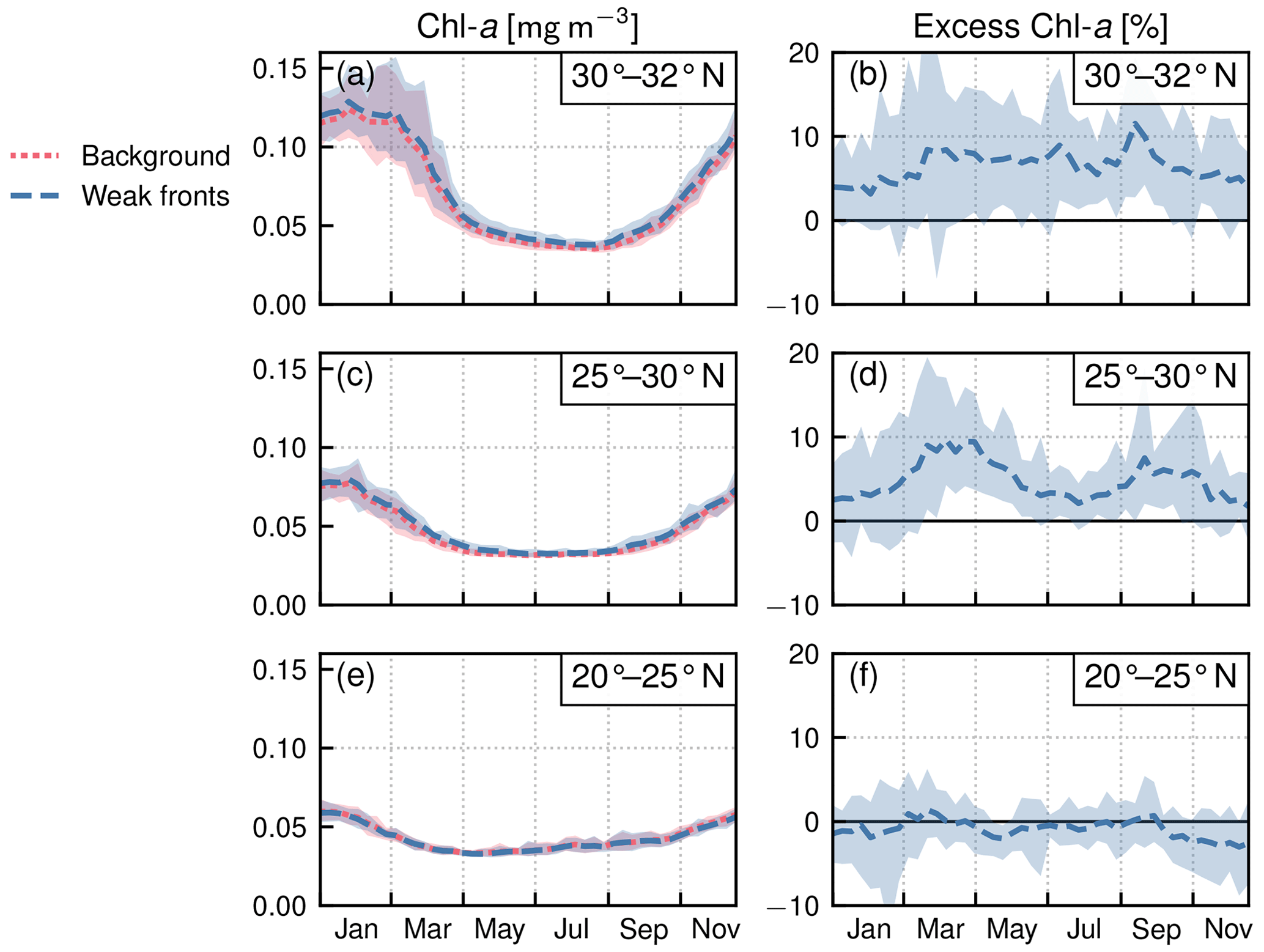
Figure 6 Permanent subtropical biome: local Chl a excess over fronts by range of latitudes. (a, c, e) Chl a median values over weak fronts (blue) and background (red). (b, d, f) Corresponding local excess of Chl a in weak fronts computed as the relative difference in Chl a in fronts and in the background. The plain lines represent the climatological mean, and the envelopes mark the standard deviation over the period 2000–2020. The excess increases from south to north.

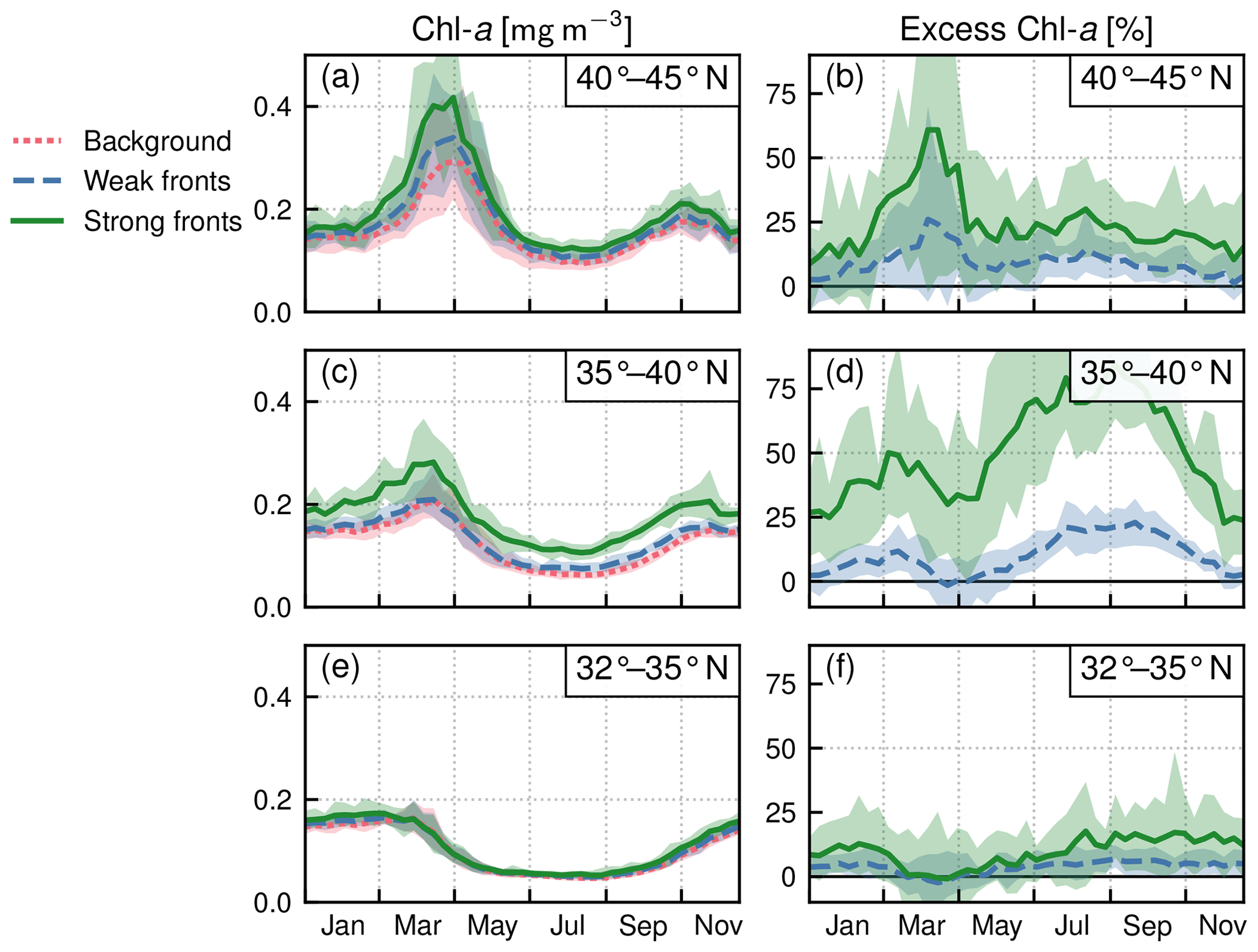
Figure 7 Seasonal subtropical biome: local Chl a excess over fronts by range of latitudes. (a, c, e) Chl a median values over weak fronts (blue), strong fronts (green), and background (red). (b, d, f) Corresponding local excess of Chl a in weak and strong fronts computed as the relative difference in Chl a in fronts and in the background. The plain lines represent the climatological mean, and the envelopes mark the standard deviation over the period 2000–2020. The excess is maximum at midlatitudes.

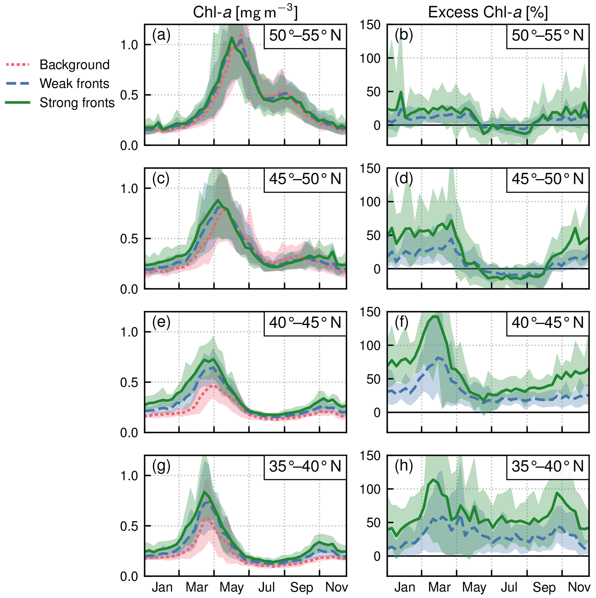
Figure 8 Subpolar biome: local Chl a excess over fronts by range of latitudes in the biome. (a, c, e) Chl a median values over weak fronts (blue), strong fronts (green), and background (red). (b, d, f) Corresponding local excess of Chl a in weak and strong fronts computed as the relative difference in Chl a in fronts and in the background. The plain lines represent the climatological mean, and the envelopes mark the standard deviation over the period 2000–2020. The excess decreases from south to north.

3.3 Biome-scale Chl a surplus associated with fronts

Within each biome, the surplus Chl a associated with the presence of fronts accounts both for the relative Chl a excess over fronts and for the relative area covered by fronts. In the permanent subtropical biome, the surplus associated with weak fronts varies between a maximum of 3 % and a minimum of zero in summer when the coverage of fronts is the lowest (Fig. 5g). The magnitude of the surplus is larger in the seasonal subtropical biome where it reaches 7 % in May for weak fronts (Fig. 5h). We can note that the surplus associated with strong fronts is much weaker despite a much greater local impact of strong fronts (Fig. 5b) due to the small surface area covered by strong fronts (Fig. 5e). The largest surplus is found in the subpolar biome, with maximum values of 12 %, due to strong fronts in March. In contrast to the seasonal subtropical biome, in the subpolar biome the surplus associated with strong fronts is larger than the surplus associated with weak fronts. Interestingly our results also reveal a Chl a deficit associated with fronts during the decay phase of the bloom and in summer (negative surplus; Fig. 5i), explained by the negative excess in the northern part of the subpolar biome (Fig. 8b–d).

Overall, the annual mean Chl a surplus due to fronts is very modest (Fig.9b). All fronts added together, the surplus is of the order of 1 % for the permanent subtropical biome and 6 % for the seasonal subtropical and subpolar biomes, with contributions from weak and strong fronts which have similar magnitudes. Therefore, there is roughly 5 % more Chl a in the Gulf Stream region than there would be in the absence of fronts.

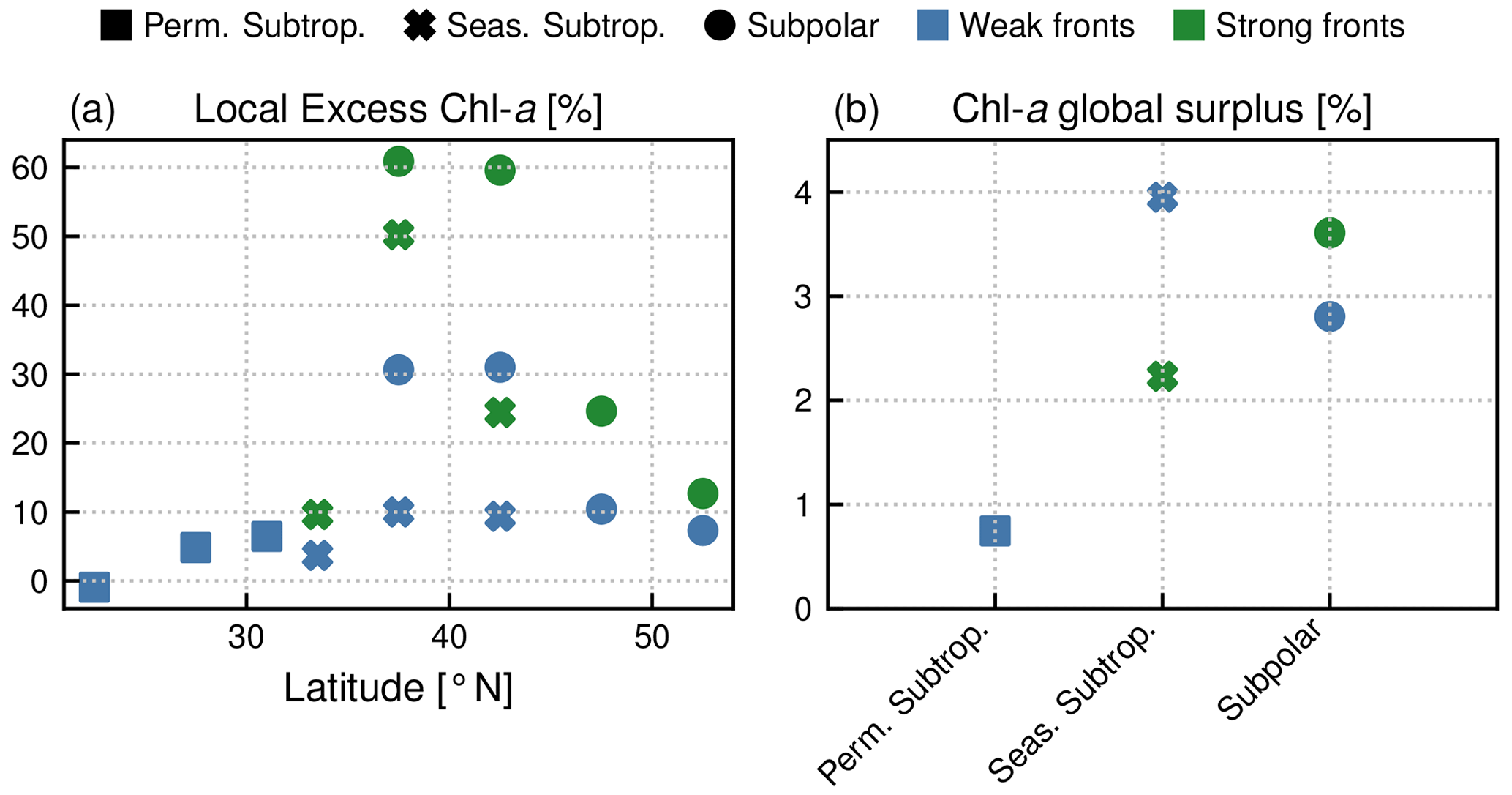
Figure 9 (a) Annual mean local Chl a excess over fronts (in %), sorted by latitudinal band (x axis), by biome (shape of symbol), and by front type (weak fronts in blue, strong fronts in green). (b) Annual mean global surplus of Chl a (in %) for each biome, sorted by front type.

3.4 Bloom timing in the subpolar biome

Another strong impact of fronts is the earlier onset of the bloom over fronts in the subpolar biome (Fig. 5c). The spring bloom onset propagates from south to north in the biome, starting in early April at 35^∘ N and in late June at 55^∘ N (Fig. 8). In all latitudinal bands, we found that the bloom onset occurs 1 week earlier over weak fronts than in the background (by $-\mathrm{6.7}\pm \mathrm{1.1}$ d) and 2 weeks earlier over strong fronts (by $-\mathrm{13.5}\pm \mathrm{1.5}$ d) (Fig. 10). There is a large spread in bloom onset dates in the 20 years of data due to the very intermittent nature of the bloom onset (Keerthi et al., 2021) that makes it difficult to detect with precision during certain years. Furthermore, in many cases no difference in bloom onset or duration could be detected between the fronts and the background (dots aligned on the diagonal in Fig. 10). Nevertheless, for individual years, delays larger than 1 month could occur.

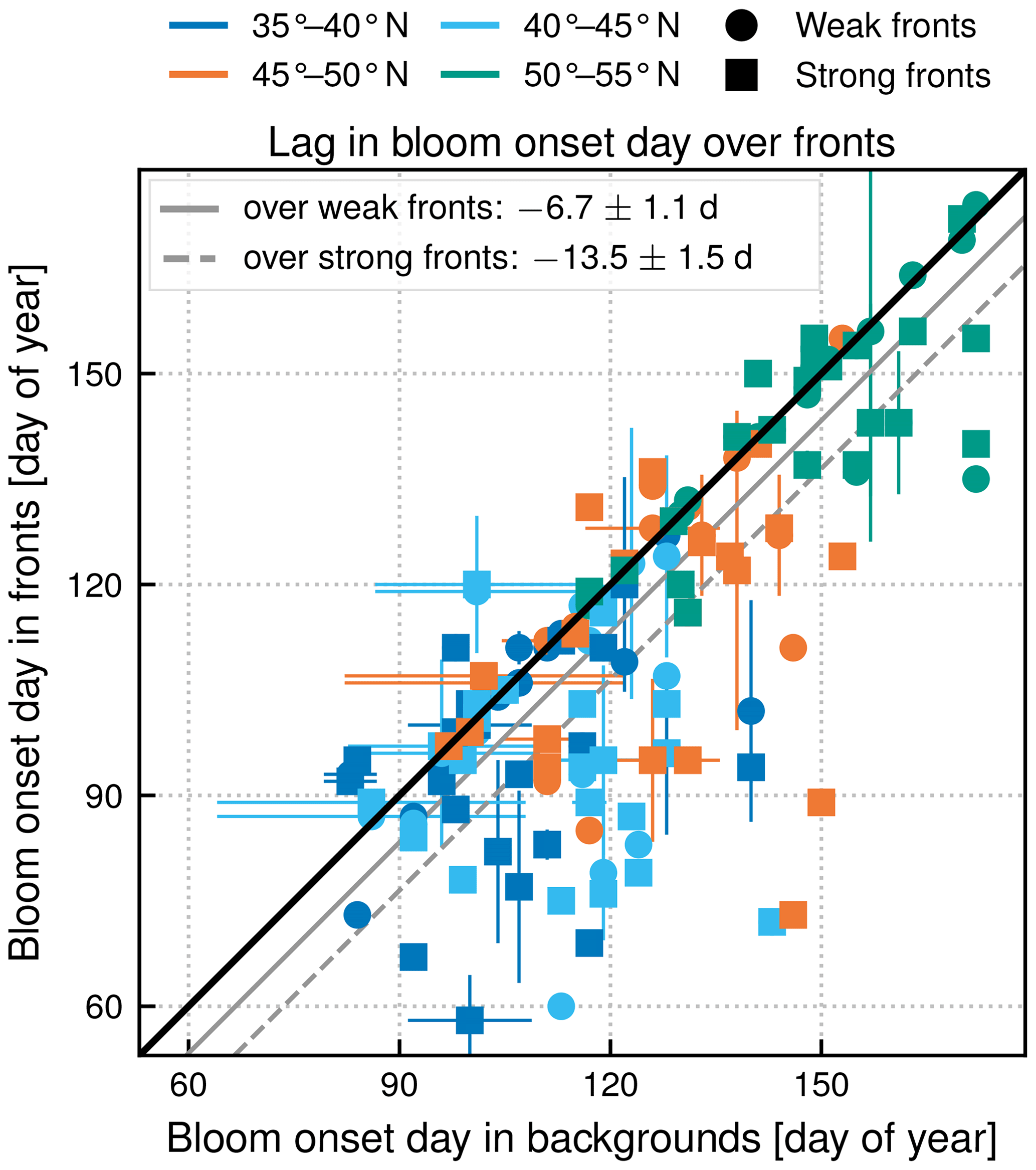
Figure 10 Subpolar biome. Comparison of bloom onset dates (in day of year) in the background (x axis) and over fronts (y axis), sorted by strength of fronts (shape of symbol) and latitudinal band (color). The line y=x is plotted in black. The distance between the black line and the plain (dashed) grey line is the measure of the average difference between weak (strong) fronts and background. The bloom onset day propagates from south to north and starts earlier over fronts at all latitudes in the subpolar biome.

4 Discussion

Our analyses of surface satellite data over the open ocean in the Gulf Stream extension region, based on the computation of an heterogeneity index (HI), allowed us to show a substantial local excess of surface Chl a concentrations over SST fronts compared to background levels, to detect earlier blooms by 1 to 2 weeks over fronts, and to quantify that the regional surplus in surface Chl a at the scale of the region associated with fronts was less than 5 %. The background levels in this region are very contrasted seasonally and geographically, with a productive and highly seasonal subpolar biome north of the Gulf Stream, a more steady oligotrophic permanent subtropical biome to the south, and an intermediate situation in between the two, where a seasonal subtropical biome prevails. The main results above hold for these three contrasted biomes, although with different intensities, which also depend on the strength of HI.

4.1 Caveats

The level 4 SST product used in this study has the advantage of being readily available on download platforms (here CMEMS) at a reasonably high spatial resolution (4 km), avoiding the need to regrid as was done in Liu and Levine (2016), who used 1 km resolution L2 MODIS Aqua data. It also has an excellent spatial coverage (e.g., Fig. 1) as it includes merged data from several sensors, but there is a trade-off between coverage and resolution. We have performed initial tests to investigate the differences in using 1 km and 4 km resolution SST data, which convinced us that the use of 4 km resolution data was appropriate (not shown), particularly since the HI is computed here over boxes of 30 km × 30 km. Nevertheless a more in-depth study of the sensitivity of our results to the resolution of the satellite products could be carried out in the future.

Another caveat of this level 4 product is that the spatial interpolation performed to merge data from several sensors smooths out the finer features, particularly when some of the data are obstructed by clouds. Here we somehow avoided these smoothed areas by using only cloud-free Chl a pixels. Nevertheless, a bias remains in that there may be a positive correlation between areas with fronts and the presence of clouds. This is the case over the Gulf Stream jet, where dramatic surface temperature gradients are found, and constant clouds are detected over the front. Similar effects can be expected over smaller, short-lived fronts but probably on a smaller scale.

Our evaluation of the regional surplus in Chl a associated with fronts assumes that the local Chl a excess due to fronts is only located over fronts. However, the localization of the highest Chl a does not perfectly coincide with elevated values of HI; there are places where the HI is large and Chl a is small, and there are also places with elevated patches of Chl a outside HI contours (see, for example, in Fig. 2). The apparent mismatch between the exact location of fronts at a given time and the exact location of the Chl a response to frontal dynamics at the same time may be due to different factors, such as the very dynamic nature of fronts which can lead to the chaotic advection of phytoplankton (and/or nutrients) outside of fronts (Abraham, 1998), the timescale needed for phytoplankton to respond to nutrient supplies at fronts, or trophic interactions at the front (as shown, for instance, in the modeling study of Mangolte et al., 2022). This implies that part of the excess Chl a attributable to frontal activity may actually be located outside of fronts. Our results show that the median distributions of Chl a significantly differ over fronts and outside of fronts, which suggests that most of the signal due to fronts actually occurs over fronts; nevertheless our estimate of the regional impact of fronts is likely an underestimate due to the signal located outside of fronts.

Moreover, our assessment of the effect of fronts on phytoplankton, based on surface Chl a, is probably a lower estimate given that the episodic nutrient injections due to submesoscale vertical velocities at fronts can get consumed before reaching the surface (Johnson et al., 2010), leading to phytoplankton enhancements that often do not reach the surface and are more intense at the subsurface (Mouriño et al., 2004; Ruiz et al., 2019). In addition, there may be photo-inhibition which prevents phytoplankton from being near the surface in oligotrophic regions, even though they may be impacted by frontal motions.

Finally, the ratio of Chl a to total phytoplankton biomass in carbon, Chl a : C, changes under varying environmental conditions and community changes (Behrenfeld et al., 2015; Halsey and Jones, 2015; Inomura et al., 2022). Diatoms exhibit higher Chl a : C ratios and are more prevalent in fronts and thus would tend to make our biomass surplus estimation overestimated (Tréguer et al., 2018). This uncertainty could be restricted by taking advantage of recent advances in synoptic estimations of the phytoplankton functional type concentrations (El Hourany et al., 2019).

We should also note that our estimates are sensitive to the method used to detect fronts. Here, we used a 30 km wide window to compute HI, while Liu and Levine (2016) used a 10 km wide window. We used a wider window in order to detect the wider western boundary current fronts. But finer ephemeral fronts dominate in oligotrophic gyres. Thus the phytoplankton signal at fronts may be underestimated with the use of a wider window there. This difference may explain why our assessment of the excess Chl a in the North Atlantic subtropical gyre is 3 times lower than the assessment of Liu and Levine (2016) in the North Pacific subtropical gyre. Dedicated sensitivity experiments would be needed to assess this with more certainty.

4.2 Local Chl a excess over fronts

With these caveats in mind, we find that the degree of local Chl a excess over fronts varied seasonally but mostly varied from one biome to another, with an intensity which was weaker in the more oligotrophic region, stronger between 35 and 45^∘ N, and intermediate in the subpolar biome (Fig. 9a). Moreover, the local excess of Chl a was always significantly larger over strong fronts than over weak fronts. The increase in Chl a with increasing front strength (i.e., with increasing HI; Fig. 3) is consistent with the hypothesis that phytoplankton production is amplified at fronts by an enhancement of the flux of nutrients and that this flux is stronger the stronger the front is. Strong fronts in this study coincide with the persistent fronts of the western boundary current system, which are associated both with large and deep-reaching vertical velocities (Liao et al., 2022) and with strong lateral transport of nutrients (Pelegrí et al., 1996). On the other hand, the larger dispersion in the Chl a distribution with increasing HI reflects the fact that not all fronts are equally efficient.

Co-occurrence between frontal vertical velocities (or divergence) and enhanced Chl a has been observed over specific fronts in the North Atlantic (Mouriño et al., 2004; Allen et al., 2005; Lehahn et al., 2007). The only study that has statistically connected enhanced Chl a with the presence of a temperature front was conducted in the North Pacific subtropical gyre (Liu and Levine, 2016), which shares characteristics with the permanent subtropical biome examined here. Our results thus extend those of Liu and Levine (2016) to a region with stronger biological contrasts and phenologies, as well as with more complex dynamics.

One of the factors determining the magnitude of the local Chl a excess over fronts is the magnitude of the vertical nutrient flux, which itself depends on the magnitude of the vertical velocities, of their depth penetration, and of the depth of the nutricline. The nutricline depth shows a sharp latitudinal gradient within this region, from 150 m depth at 25^∘ N to 50 m at 50^∘ N (Romera-Castillo et al., 2016). This can explain the maximum magnitude of the Chl a response at the northern edge of the subtropical gyre, where the lack of nutrients is more severely controlling phytoplankton abundance than further north and where the nutricline is closer to the surface than further south. Another factor that can explain this signal is the nutrient stream that feeds this intermediate regions with nutrients.

Moreover, vertical velocities associated with ephemeral fronts, often confined to the mixed layer, are likely to be a less efficient nutrient flux pathway to the euphotic zone from the interior than deep, dynamic, persistent fronts extending well below the mixed layer (Lévy et al., 2018). The contrasting impacts of deep and shallow fronts are striking in models (Lévy et al., 2012) but are difficult to quantify from a small number of in situ observations. Here we observed that the magnitude of the Chl a response over fronts increased with the strength of the HI (Fig. 3). In other words, strong fronts, characterized by high values of HI (HI>10), led to a stronger increase in Chl a values than weak fronts, characterized by intermediate values of HI ($\mathrm{5}<\text{HI}<\mathrm{10}$).

Finally, an important outcome of this study is that the surplus in phytoplankton biomass associated with fronts can be stronger in blooming biomes than in oligotrophic ones. In fact in regions where nutrients are not limiting productivity, fronts have been shown to subduct excess nutrients (Oschlies, 2002; Gruber et al., 2011) and excess biomass (Lathuilière et al., 2010) rather than to lead to an increase in biomass as in oligotrophic regions. This effect of a decreased biomass, suggestive of subduction, is observed here in the northern parts of the subpolar biome between May and September (Fig. 8b–d). But we also find that in the subpolar biome, the Chl a excess over fronts can reach 150 % during the bloom and 50 % during summer (Fig. 8), while in the permanent subtropical biome it never exceeds 10 % (Fig. 6). The enhancement of the spring bloom by submesoscale frontal processes observed here was recently also put forward in a modeling study by Simoes-Sousa et al. (2022).

4.3 Persistent and ephemeral fronts

The above results are suggestive that the heterogeneity index could be used as a way to discriminate between persistent (and deep) fronts and ephemeral (and shallower) fronts. The localization and frequency of strong and weak fronts is consistent with this hypothesis. Weak fronts are much more frequent than strong fronts, as we expect from ephemeral fronts compared with persistent ones (Fig. 4). In addition, the localization of strong fronts coincides with the position of the Gulf Stream and shelf-break front. Another element that supports this hypothesis is the scale over which the HI is computed (30 km) which gives a strong weight to SST heterogeneities associated with large contrasts, which is the case across the Gulf Stream and shelf break. Of course, more direct evidence linking the penetration of fronts with the intensity of the heterogeneity index would be needed to confirm the association.

4.4 Biome-scale Chl a amplification associated with fronts

The categorization of fronts based on HI has allowed us to quantify the respective contribution of two types of fronts on the regional Chl a amplification (Fig. 9b). Weak fronts are associated with a local Chl a excess which is weaker than strong fronts, in general, but because they are also more frequent than strong fronts, depending on the biome and seasons, they contribute equally to the regional Chl a surplus as strong fronts. There is also some degree of seasonality in this small surplus of Chl a attributed to fronts, which heavily depends on the region of interest (Fig. 5). As predicted by theory and noted by previous studies, submesoscale fronts – which are confined to the mixed layer – are less abundant in summer when mixed layers are shallower. In the south zone, this leads to an overall weaker effect of fronts in summer (near 0 %) relative to the rest of the year (less than 3 % average), but in the jet area, it is compensated for by a larger intensity of the increase in Chl a in summer, leading to a Chl a surplus in summer (7 % for weak fronts) which is much larger than in winter (1 %). In the north, the situation is quite different with an impact of fronts close to zero during the spring bloom, negative in summer as vertical velocities at fronts are also capable of sinking the surface bloom (Lévy et al., 2018), and maximal in fall and winter.

Besides these small spatial and temporal variations in amplitude, a key result of this study is that, despite strong local impact of fronts, their overall contribution at large-scale remains small, a few percent at most, and of the order of 5 % for the entire region. Nevertheless, this result should be considered as a lower bound first because increases in Chl a at fronts are often stronger at subsurface than at the surface and second because, in a region characterized by strong gradients like this one, additional nutrient fluxes due to frontal activity might not necessarily lead to local anomalies in Chl a but could also be hidden by the large-scale gradient. Finally, 5 % amplification of surface Chl a might lead to greater amplification at higher trophic levels (Stock et al., 2014; Lotze et al., 2019), with ecological implications that remain to be evaluated.

4.5 Earlier blooms over fronts

Another key result of this study is the detection of earlier blooms over fronts than over background conditions in the north of the Gulf Stream jet. Several field and modeling studies have shown that frontal dynamics, by tilting existing horizontal density gradients, increase the vertical stratification of surface mixed layers (Taylor and Ferrari, 2011), which can lead to the stratification of the mixed layer prior to seasonal stratification. Given that the surface spring bloom is triggered by increased stratification, this effect can cause earlier local phytoplankton blooms over fronts compared to surrounding areas.

However, while the increased stratification over fronts can be directly observed in situ (Karleskind et al., 2011; Mahadevan et al., 2012), how it affects the timing of the bloom has so far only been quantified with numerical models due to the difficulty in tracking the bloom evolution over fronts which themselves evolve over time (Lévy et al., 2000; Karleskind et al., 2011; Mahadevan et al., 2012). We provide here the first observational evidence of the early onset of blooms over fronts. Moreover, our estimate leads to smaller values (earlier blooms by 1 to 2 weeks) than previously estimated from models (20–30 d by Mahadevan et al., 2012).

The method that we used to quantify differences in bloom timing over fronts and background is based on the time evolution of a Eulerian quantity (the Chl a median over latitudinal bands), whereas the bloom evolves along Lagrangian trajectories. Considering a rather small area, as we have done here, is a way of overcoming the difficulty of following the temporal evolution on fronts whose life history is too complex to be captured and shorter than the bloom itself. It also limits the impact that the northward propagation of the bloom could have on the temporal assessment. It should also be noted that it is inherently difficult to pinpoint the precise onset and end days of a bloom, as the spring bloom shows large intraseasonal variability in its characteristics; its beginning can be more or less sudden and is often made of multiple peaks (Keerthi et al., 2020).

5 Conclusions

The open-ocean Gulf Stream extension region is a region of strong biological contrasts and the particularly strong frontal activity of the world's ocean, undergoing rapid warming which strongly affects fisheries (Pershing et al., 2015; Neto et al., 2021). Quantifying the impact of fronts on phytoplankton is thus particularly relevant, and we expected to detect a large impact. The use of 20 years of satellite data of SST to detect fronts and of surface Chl a to compute anomalies over the front allowed us to provide a robust assessment of this impact. We found three main results: first, that the regional increase in surface phytoplankton associated with fronts is rather modest, 5 % at most; second, that nutrient supplies at fronts enhanced the spring bloom 2 to 3 times more than they enhanced oligotrophic regions; and third, that the spring bloom onset was earlier over fronts by 1 to 2 weeks, which we already knew from models (Karleskind et al., 2011; Mahadevan et al., 2012) but for which we had no direct evidence nor sound quantification. We also showed a reduction in phytoplankton over fronts at the end of the bloom, which we attributed to subduction.

Although limited to the Gulf Stream region, this study provides a well-tested methodology that could enable the study of the links between small-scale ocean physics and phytoplankton response in other regions of the global ocean. In addition, these results on the importance of fronts for phytoplankton biomass and phenology could also be used to evaluate models coupling ocean physics and phytoplankton at high spatial resolution or to test parameterizations representing the effect of small scales on phytoplankton production in coarser-resolution models. Finally, the combination of these observation-based results with theoretical arguments and well-assessed models should also allow us to better constrain the response of phytoplankton production to climate change (Couespel et al., 2021), which still has very large uncertainties, as shown by the latest set of Earth system models (Kwiatkowski et al., 2020).

Appendix A:  

Figure A1 Climatological mean of Chl a median values (a, b, c) over weak fronts (blue), strong fronts (green), and background (red); surface fraction occupied by weak fronts and strong fronts (d, e, f); and global Chl a excess due to weak and strong fronts (g, h, i). Each line represents a set of parameters with the bolder line indicating the retained set of parameters. The tested rolling window sizes are 20, 30, and 40 km. Different normalization coefficients are tested for a 30 km window size: double the variance, double the bimodality, and double the skewness.

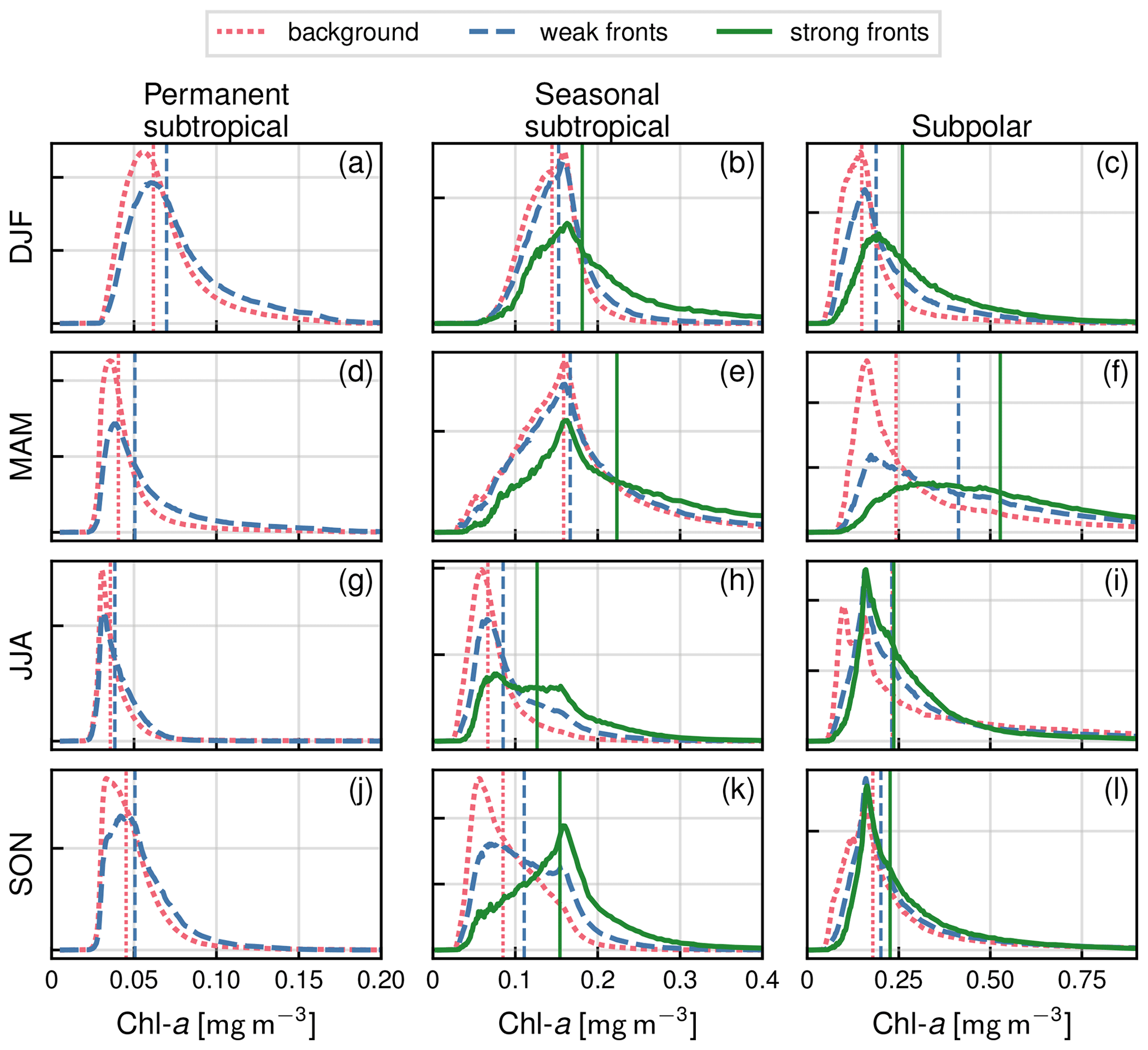
Figure A2 Distribution of Chl a of the year 2007 by seasons (rows) and for the three biomes (columns), as well as for the background (red), weak fronts (blue), and strong fronts (green). The median value of each distribution is indicated by a vertical line.