Assessing global-scale organic matter reactivity patterns in marine sediments using a lognormal reactive continuum model

Organic matter (OM) degradation in marine sediments is largely controlled by its reactivity and profoundly affects the global carbon cycle. Yet, there is currently no general framework that can constrain OM reactivity on a global scale. In this study, we propose a reactive continuum model based on a lognormal distribution (l-RCM), where OM reactivity is fully described by parameters μ (the mean reactivity of the initial OM bulk mixture) and σ (the variance of OM components around the mean reactivity). We use the l-RCM to inversely determine μ and σ at 123 sites across the global ocean. The results show that the apparent OM reactivity ($\langle k\rangle =\mathit{\mu }\cdot \exp ({\mathit{\sigma }}^{\mathrm{2}}/\mathrm{2})$) decreases with decreasing sedimentation rate (ω) and that OM reactivity is more than 3 orders of magnitude higher in shelf than in abyssal regions. Despite the general global trends, higher than expected OM reactivity is observed in certain ocean regions characterized by great water depth or pronounced oxygen minimum zones, such as the eastern–western coastal equatorial Pacific and the Arabian Sea, emphasizing the complex control of the depositional environment (e.g., OM flux, oxygen content in the water column) on benthic OM reactivity. Notably, the l-RCM can also highlight the variability in OM reactivity in these regions. Based on inverse modeling results in our dataset, we establish the significant statistical relationships between 〈k〉 and ω and further map the global OM reactivity distribution. The novelty of this study lies in its unifying view but also in contributing a new framework that allows predicting OM reactivity in data-poor areas based on readily available (or more easily obtainable) information. Such a framework is currently lacking and limits our abilities to constrain OM reactivity in global biogeochemical or Earth system models.

1 Introduction

Marine sediments act as the ultimate sink for organic carbon. The size and reactivity of the benthic organic matter (OM) reservoir are a critical component of the global carbon cycle (Arndt et al., 2013). In particular, the reactivity of benthic OM imposes a substantial control on the magnitude of benthic carbon burial over geological timescales due to the recycling of organic carbon by dissimilatory microbial activity in the deep biosphere (Boudreau, 1992; Zonneveld et al., 2010), the dissolution and precipitation of carbonates (Meister et al., 2022; Nöthen and Kasten, 2011), and the production of methane (Dickens et al., 2004; Whiticar, 1999). Decades of research have shown that OM reactivity is controlled by both the nature of the OM (origin, composition and degradation state) and its environmental and depositional conditions (e.g., redox conditions, sedimentation rate, mineral protection, microbial community composition and biological mixing) (Burdige, 2007; Egger et al., 2018; Hartnett et al., 1998; Hedges and Keil, 1995; Larowe et al., 2020a; Zonneveld et al., 2010). However, due to the complex and dynamic nature of the main controls on OM reactivity, the specific relative significance of these controlling factors remains poorly quantified. Consequently, OM degradation models generally do not explicitly describe the influence of environmental and depositional factors on OM reactivity and its evolution but rather apply simplified parametrizations (Freitas et al., 2021; Pika et al., 2021). Over the past decades, several models have been developed and successfully used to quantify OM degradation in marine sediments. They can be broadly divided into two groups: discrete models, such as the (multi-) G model (Berner, 1964; Jørgensen, 1978), and continuum models, such as the reactive continuum model (RCM) (Boudreau and Ruddick, 1991) and the power model (Middelburg, 1989).

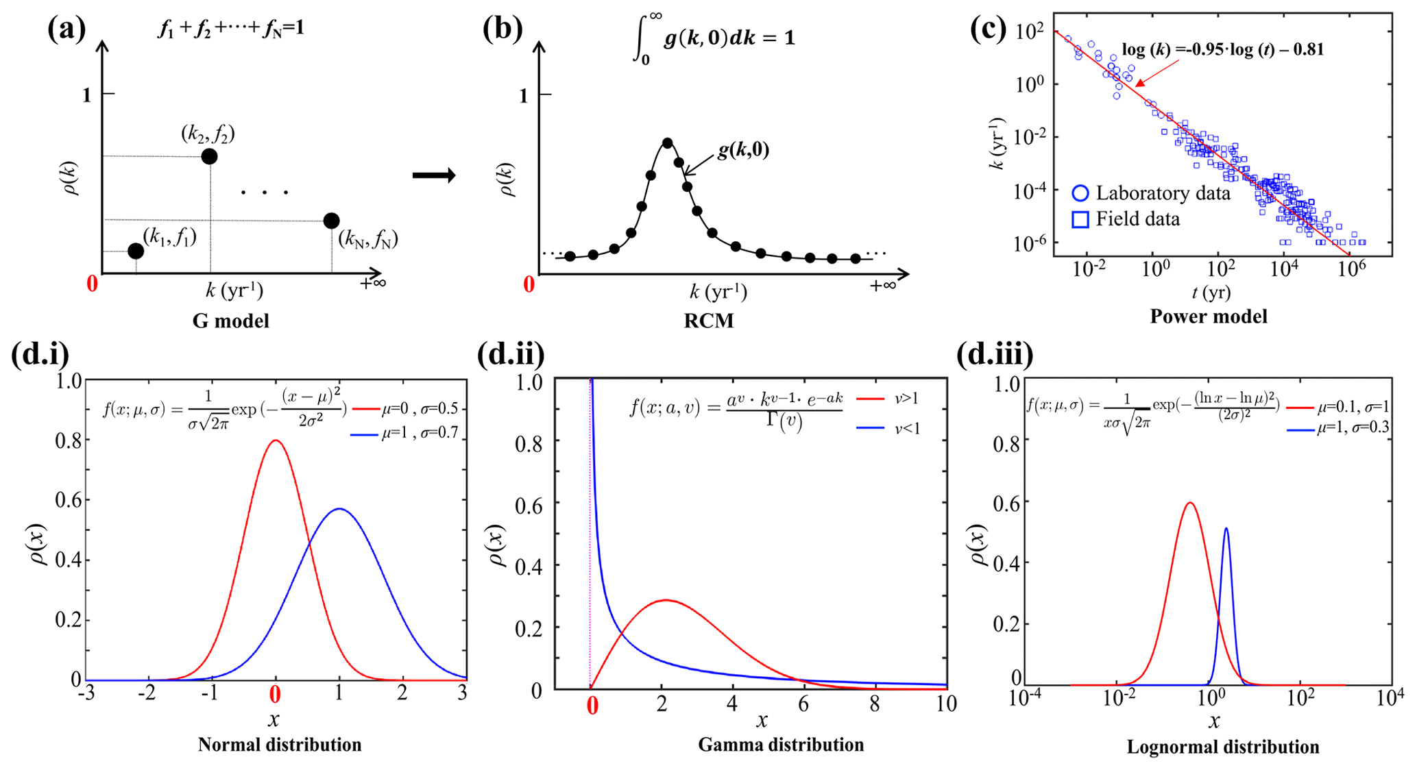
Figure 1 Schematic diagram of different OM degradation models. (a) G model, (b) RCM, (c) Power model and (d) Common continuum distribution functions. The x coordinate denotes the variation range of values, and the y coordinate denotes the probability density distribution (ρ) (i. the normal distribution, a typical all-axis distribution; ii. the gamma distribution, a typical semi-axis (x > 0) distribution; and iii. the lognormal distribution, a typical semi-axis (x > 0) distribution).

Discrete models divide the bulk OM pool into several discrete fractions, each with its own constant reactivity (Fig. 1a). The 1-G model is the earliest OM degradation model, which is based on the assumption that OM degrades according to first-order dynamics with a single constant degradation rate constant (Berner, 1964). The multi-G model, however, divides OM into several fractions, and each fraction is degraded according to a first-order rate with a fraction-specific reactivity (Jørgensen, 1978). Although multi-G models successfully fit observed OM degradation dynamics when comprehensive datasets are available, their application on a global scale is complicated by the need to partition the OM reactivity into a finite number of fractions and define their reactivities. A multi-G model with n discrete OM fractions requires constraining 2n−1 parameters and is, thus, over-parametrized (Jørgensen, 1978). Nevertheless, because of its mathematical simplicity and wide use, multi-G models have been used in a range of diagenetic models designed for the global or regional scale (e.g., CANDI, MEDIA, MEDUSA and OMEN SED; Boudreau, 1996; Meysman et al., 2003; Munhoven, 2007; Pika et al., 2021). Constraining the 2n−1 OM degradation model parameters for these global-scale applications is not straightforward. Early strategies for constraining the reactivity of OM on a global scale have focused on deriving empirical relationships between OM reactivity and single, easily observable characteristics of the depositional environment (water depth, sedimentation rate or OM flux) (Arndt et al., 2013). However, a poor statistically significant link between OM reactivity and depositional environment could be established (R²<0.1) after compiling published multi-G model parameters across a wide range of depositional environments, model complexities, sediment depths, and burial timescales (Arndt et al., 2013).

Reactive continuum models (RCMs) are an alternative to discrete models. They assume that OM compounds are continuously distributed over a wide range of reactivities. The degradation rate can be described as the sum of an infinite number of discrete fractions, each degraded according to first-order kinetics (Boudreau and Ruddick, 1991), as

$$\begin{array}{}\text{(1)}& G\left(t\right)=\underset{\mathrm{0}}{\overset{\mathrm{\infty }}{\int }}G\left(\mathrm{0}\right)\cdot g(k,\mathrm{0})\cdot e^{-kt}\mathrm{d}k,\end{array}$$

where G(t) is OM content at time t, G(0) is OM content at the sediment–water interface (SWI), k is the first-order degradation rate constant, and g(k,0) is the initial reactivity distribution of OM at the SWI. The key to constructing an RCM is to select a continuum distribution that describes the OM reactivity at the SWI (Fig. 1b). Considering the k value in Eq. (1) must be greater than zero (k>0), some of the all-axial statistical distributions ($x\in (-\mathrm{\infty },+\mathrm{\infty })$) are not appropriate for constructing RCMs (e.g., normal distribution; Fig. 1d.i). Boudreau and Ruddick (1991), following Aris (1968) and Ho and Aris (1987), proposed using a gamma distribution (γ-RCM; Fig. 1d.ii) due to its mathematical properties and its ability to capture the observed dynamics:

$$\begin{array}{}\text{(2)}& g(k,\mathrm{0})={\displaystyle \frac{a^v\cdot k^{v-\mathrm{1}}\cdot e^{-ak}}{\mathrm{\Gamma }\left(v\right)}},\end{array}$$

where a is the average age of the OM at the SWI, v is the shape parameter, and Γ(v) is the gamma function. In addition, Middelburg (1989) empirically derived a power law from a large data compilation of measured OM reactivity (Fig. 1c), which is mathematically equivalent to the γ-RCM. The advantage of the continuum models over the discrete models is that they merely require constraining two free parameters to capture the widely observed continuous decrease in OM reactivity with degradation time and depth. Recently, the γ-RCM has been used to inversely determine the free γ-RCM parameters, and thus benthic OM reactivity, from observed particulate organic carbon (POC) and sulfate depth profiles across a wide range of different depositional environments (Freitas et al., 2021). Although results revealed broad global patterns, no significant statistical relationship (R²<0.46) between the parameters (a and v) of the γ-RCM (Arndt et al., 2013) and characteristics of the depositional environment could be found, and constraining OM degradation model parameters on the global scale thus remains difficult.

Here, we present an RCM based on a lognormal distribution (Forney and Rothman, 2012b):

$$\begin{array}{}\text{(3)}& g(k,\mathrm{0})={\displaystyle \frac{\mathrm{1}}{k\cdot \mathit{\sigma }\cdot \sqrt{\mathrm{2}\mathit{\pi }}}}\cdot e^{-(\ln k-\ln \mathit{\mu }{)}^{\mathrm{2}}/(\mathrm{2}{\mathit{\sigma }}^{\mathrm{2}})},\end{array}$$

where ln μ is the mean of ln k, and σ² is the variance of ln k (Fig. 1d.iii). Parameter μ determines the mean reactivity of the initial OM bulk mixture, and parameter σ reflects the spread of OM components around the mean reactivity.

The lognormal distribution is formed by the multiplicative effects of random variables, which are commonly observed in nature (e.g., the radioactivity of elements in the crust, the incubation period of infectious diseases and ecological species abundance) (Limpert et al., 2001). In the ocean system, the rates of ocean primary production and biological carbon export also fit the lognormal distribution (Cael et al., 2018). The degradation of OM in natural ecosystems is controlled by a network of biologically, physically and chemically driven processes (Forney and Rothman, 2014), so the variables raised from such multiplicative processes are often followed by a lognormal distribution. Forney and Rothman (2012b) showed that litter bag OM incubation data are indeed best described by a lognormal distribution of rates.

In this study, we first compared the l-RCM with other OM degradation models and analyzed the advantages of the l-RCM in describing the OM reactivity distribution. Then we simulated OM degradation in marine sediment at 123 global sites using the l-RCM. Based on inverse modeling results in our dataset, we established the empirical formulas of OM reactivity vs. sedimentation rate and further mapped the global OM reactivity distribution. This study provides a new framework for assessing OM reactivity on regional and global scales and predicting OM reactivity in data-poor areas based on easily obtainable environmental parameters (e.g., sedimentation).

2 Materials and methods

2.1 OM degradation model approach

We constructed an RCM with lognormal distribution (l-RCM) to simulate the OM degradation in marine sediments. The g(k,0) we used in Eq. (1) is the lognormal distribution (Eq. 3). Because of the tail of g(k,0), the mean rate constant for bulk OM degradation or the apparent degradation rate of the bulk OM (〈k〉) is written as follows:

$$\begin{array}{}\text{(4)}& \langle k\rangle =\underset{\mathrm{0}}{\overset{\mathrm{\infty }}{\int }}k\cdot g(k,\mathrm{0})\mathrm{d}k=\mathit{\mu }\cdot e^{{\mathit{\sigma }}^{\mathrm{2}}}/\mathrm{2}.\end{array}$$

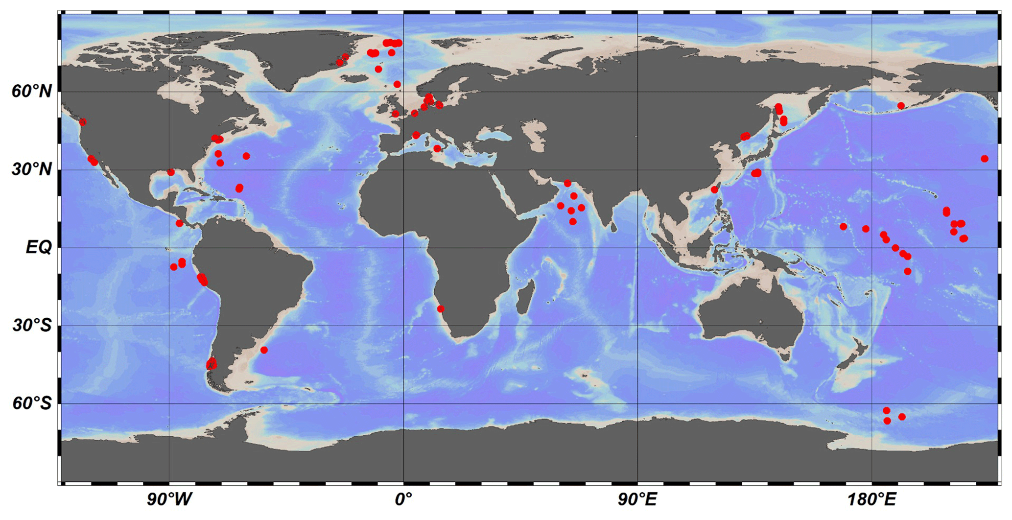
Figure 2 Global distribution of investigated sites.

2.2 Inverse model approach

Here, we used 123 published datasets of OM depth profiles across a wide range of different depositional environments that have been sourced from published literature (Middelburg, 1989; Arndt et al., 2013; Middelburg et al., 1997) and the IODP (International Ocean Discovery Program) database (Fig. 2, Table S1 in the Supplement) to inversely determine the μ and σ parameters. We also analyzed several groups (n=12) of laboratory experiment data on OM degradation (Middelburg, 1989), as well as OM degradation datasets (n=16) from terrestrial soils (Katsev and Crowe, 2015). We followed the inverse modeling approach by Forney and Rothman (2012a) to identify the best-fitting parameters μ and σ based on the Newton method.

Notably, the burial time was correlated with the porosity. A simple exponential function was used to describe porosity in sediments:

$$\begin{array}{}\text{(5)}& \mathit{\phi }\left(x\right)={\mathit{\phi }}_{\mathrm{0}}\cdot e^{-\mathit{\lambda }x},\end{array}$$

where φ₀ is the value of porosity at the SWI, λ is the attenuation coefficient, and x is depth. Considering the compaction impacts on OM degradation, the burial time corresponding to each depth in the OM profile can be calculated as

$$\begin{array}{}\text{(6)}& t\left(x\right)=\underset{\mathrm{0}}{\overset{x}{\int }}{\mathit{\omega }}^{-\mathrm{1}}\mathrm{d}x={\displaystyle \frac{x}{{\mathit{\omega }}_f}}+{\displaystyle \frac{({\mathit{\phi }}_{\mathrm{0}}-{\mathit{\phi }}_f)}{(\mathrm{1}-{\mathit{\phi }}_f)\cdot \mathit{\lambda }\cdot {\mathit{\omega }}_f}}\cdot (e^{-\mathit{\lambda }\cdot x}-\mathrm{1}),\end{array}$$

where φ_f is the value of porosity at larger depths, calculated from Eq. (5) and the pre-set simulation depth. If the porosity data were not available, the setting of porosity in global sediments was as follows: shelf regions (φ₀: 0.45, λ: 0.5 × 10⁻³), slope regions (φ₀: 0.74, λ: 1.7 × 10⁻⁴) and abyssal regions (φ₀: 0.7, λ: 0.85 × 10⁻³) (LaRowe et al., 2020b).

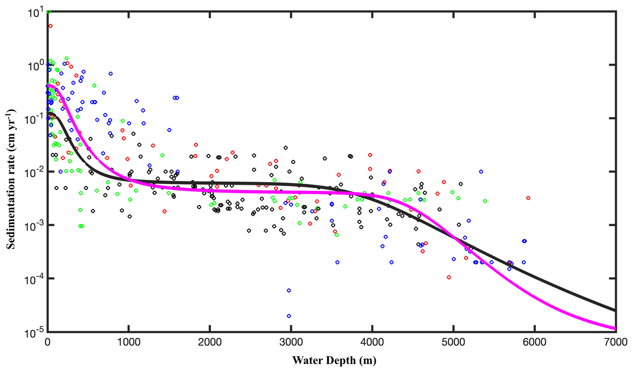
Figure 3 Relationship between sedimentation rate (w) and water depth (z in m). The data are taken from Arndt et al. (2013) (black circles), Egger et al. (2018) (pink circles), Betts and Holland (1991) (red circles), Colman and Holland (2000) (green circles), and Seiter et al. (2004) (blue circles). The pink line is the fitting result according to Eq. (8) (R²=0.57), and the black line is the fit obtained from the data of Burwicz et al. (2011) (R²=0.43).

2.3 Global upscaling of sedimentation rate

The inversely determined μ and σ couples of all investigated sites were then used in a linear regression method to derive the empirical relationships between OM parameters μ, σ and 〈k〉 and the local sedimentation rates (ω). A correction factor (f_c; Eq.7) was applied to calculate the skewness bias inherent in the back conversion from a log–log-transformed linear regression model to arithmetic units (Egger et al., 2018; Middelburg et al., 1997):

$$\begin{array}{}\text{(7)}& f_{\mathrm{c}}=e^{\mathrm{2.65}\times s^{\mathrm{2}}},\end{array}$$

where s² is the variance of the model residuals. The newly derived empirical relationships between 〈k〉 and ω were then used to calculate global maps of OM reactivity at the SWI on a 1^∘ × 1^∘ grid cell of the world ocean. At each grid point, ω was estimated based on the empirical relationship between ω (ω in cm yr⁻¹) and the water depth (z in m) (Eq. 8, Fig. 3), derived from 260 observations on the global continental shelves (Burwicz et al., 2011), complemented here by an extra 360 sites including abyssal regions (data from Arndt et al., 2013; Egger et al., 2018).

$$\begin{array}{}\text{(8)}& \mathit{\omega }\left(z\right)={\displaystyle \frac{\mathrm{0.4}}{\mathrm{1}+{\left(\frac{z}{\mathrm{200}}\right)}^{\mathrm{3.5}}}}+{\displaystyle \frac{\mathrm{0.004}}{\mathrm{1}+{\left(\frac{z}{\mathrm{4500}}\right)}^{\mathrm{17}}}}\end{array}$$

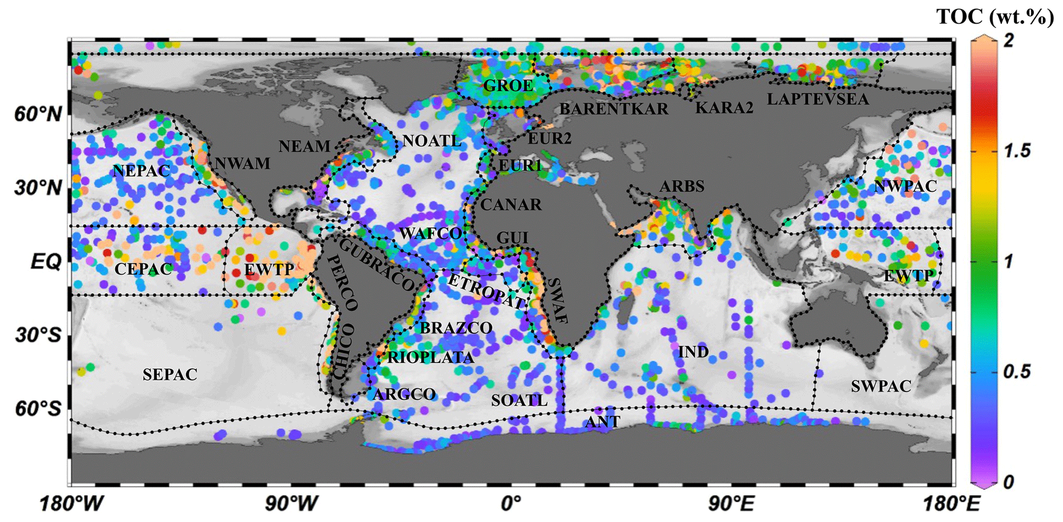
Figure 4 The 30 different regions of the global ocean were divided using 5600 single measured data points of OM content (wt %) of surface sediments. TOC signifies total organic carbon.

Considering the geographic differences in depositional environments and to describe the global distribution of sedimentary OM reactivity in more detail, we divided the global ocean into 30 different regions (Table 2, Fig. 4) using 5600 single measured data points of OM content in global surface sediment (< 5 cm sediment depth) and the previously used combined qualitative and quantitative geostatistical methods (Seiter et al., 2004).

Table 1 List of model parameters and coefficients of determination (R²) for the fitting result of γ-RCM and l-RCM.

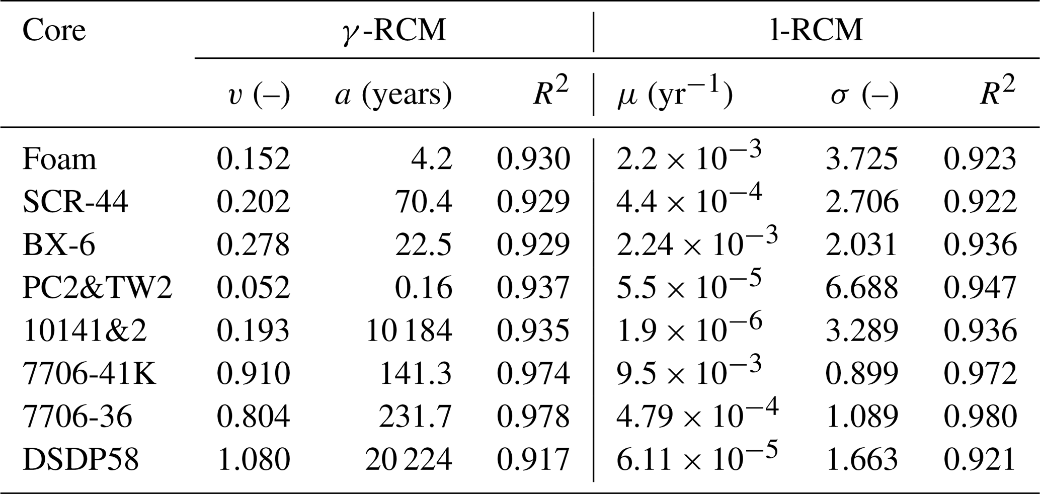
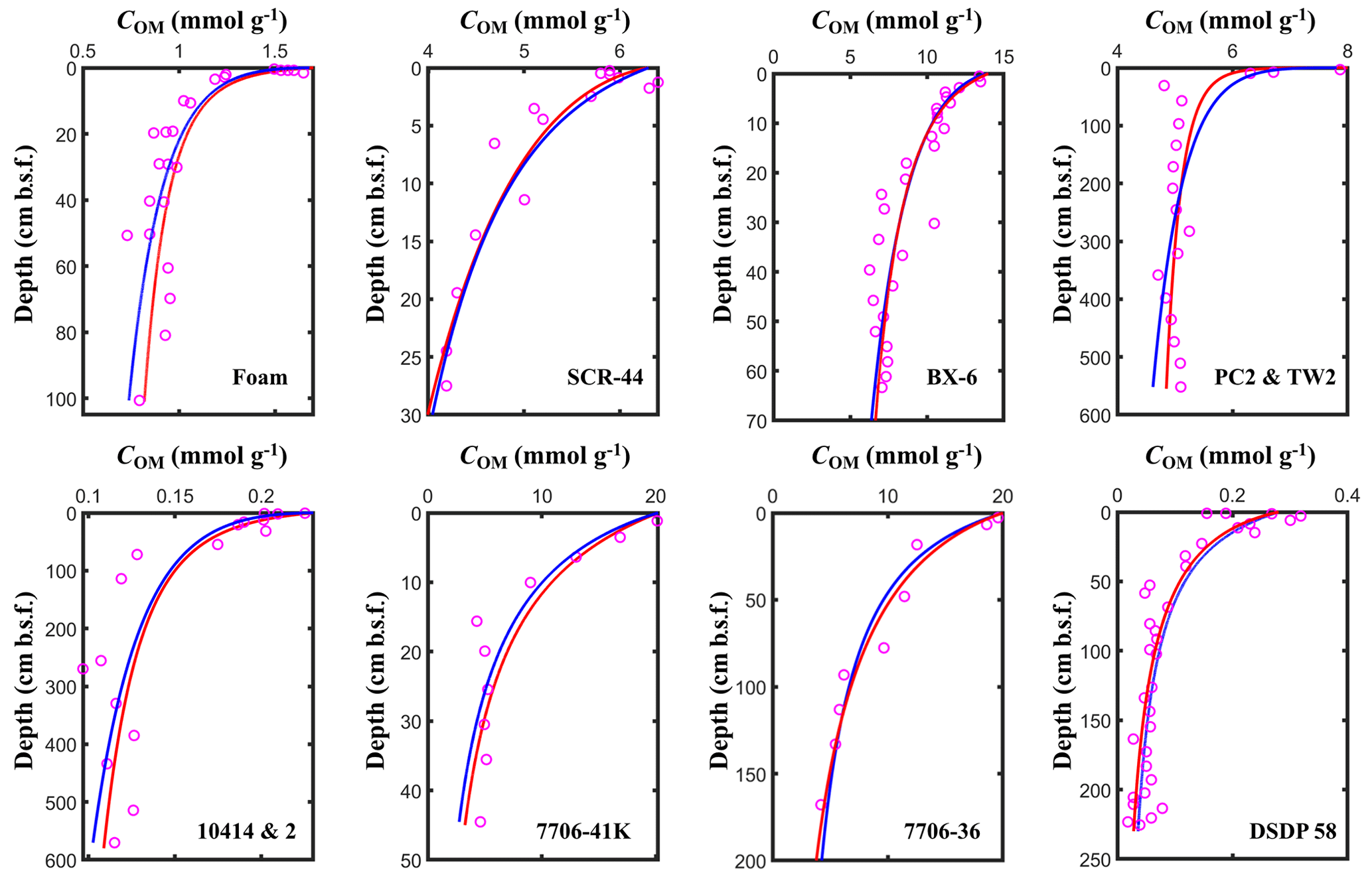
Figure 5 Fitting results of the l-RCM and the γ-RCM. The pink dots are the measured OM data, the red lines are the l-RCM fitting results, and the blue lines are the γ-RCM fitting results.

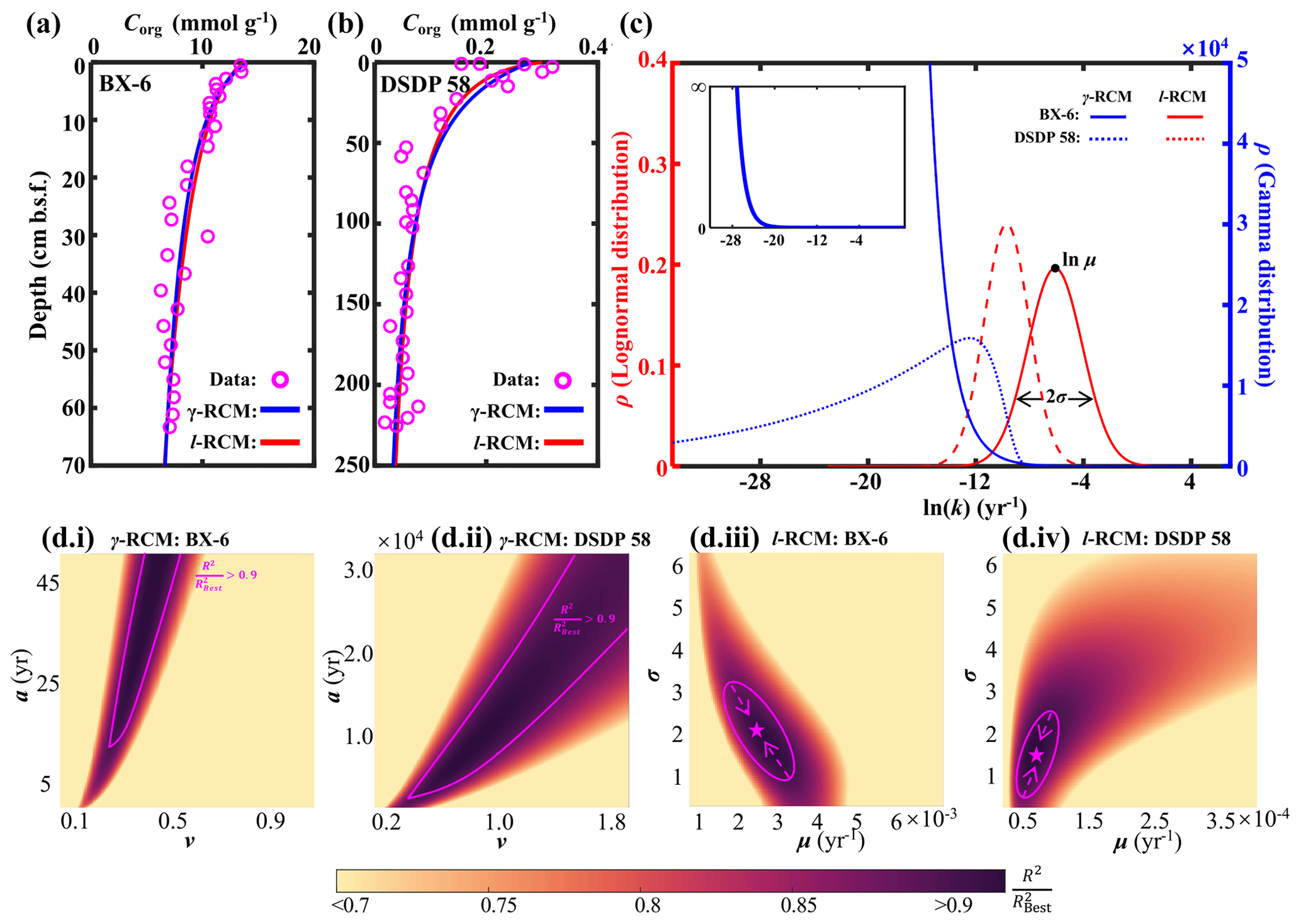
Figure 6 Comparison of the l-RCM and the γ-RCM. (a, b) The fitting results of the l-RCM and the γ-RCM for sites BX-6 and DSDP 58. (c) OM reactivity distribution from the l-RCM and the γ-RCM. Top inset, gamma distribution at site BX-6 with a larger y axis. (d) Distribution of $R^{\mathrm{2}}/R_{\mathrm{Best}}^{\mathrm{2}}$ for parameter sensitivity analysis of the γ-RCM and the l-RCM at sites BX-6 and DSDP 58. The pink lines in (i) and (ii) denote the range that $R^{\mathrm{2}}/R_{\mathrm{Best}}^{\mathrm{2}}$ is greater than 0.9 in the γ-RCM. The $R^{\mathrm{2}}/R_{\mathrm{Best}}^{\mathrm{2}}$ in the l-RCM converges as the pink arrows in (iii) and (iv), ultimately reaching the best fitting results as the pink pentagrams.

3 Results and discussion

3.1 OM reactivity distribution described by the γ-RCM and the l-RCM

To compare OM reactivity distribution described by the l-RCM and the γ-RCM, we determined the best fit to the eight OM datasets reported by Boudreau and Ruddick (1991). The results show that both RCMs fit the data equally well, as illustrated by the high coefficient of determination for each fit (R² > 0.9; Table 1 and Fig. 5). However, the l-RCM and the γ-RCM differ in their ability to find a unique solution and in their respective probability density functions of OM reactivity (ρ(k)). For example, Fig. 6a and b show the best-fit OM profiles for two contrasting sites: BX-6 on the shelf and DSDP 58 in the abyssal region. The inversely determined parameters at the two sites are μ = 2.23 × 10⁻³ yr⁻¹ and σ = 2.03 at BX-6 and μ = 6.11 × 10⁻⁵ yr⁻¹ and σ = 1.66 at DSDP 58 by the l-RCM. At BX-6, the best-fitting parameters by the γ-RCM are v = 0.278 and a = 22.5 and at DSDP 58 v = 1.08 and a = 20 224. According to the parameter sensitivity analysis, the R² of the fitted results remains greater than 0.9 when a and v change substantially simultaneously (Fig. 6d, Table S2, Figs. S1–S3 in the Supplement). As a result, different combinations of a and v can fit the data equally well. For example, simultaneously increasing v and a (v = 0.5 and a = 53) at site BX-6 or decreasing v and a (v = 0.5 and a = 4024) at site DSDP 58 leads to a slight change in R². Adding additional measured data, such as depth profiles of porewater sulfate and methane concentrations, can help in finding a unique solution (Freitas et al., 2021). In contrast, the best-fit parameters μ and σ are unique in the l-RCM, and even small changes in either parameter can lead to abysmal fitting results (Fig. 6d). The second difference between the two models concerns the shape of the probability distribution ρ(k). Statistically, the features of the gamma distribution vary with the value of v. If v < 1, ρ(k) tends to positive infinity when k approaches zero. In contrast, if v > 1, ρ(k) tends to zero when k approaches zero. Hence, the characteristics of the gamma distribution under different v values are difficult to visually compare with the OM reactivity distributions at site BX-6 (v < 1) and DSDP 58 (v > 1) (Fig. 6c). Compared with the γ-RCM, the l-RCM can better distinguish OM reactivity distribution at different sites.

3.2 Regional distribution of OM reactivity

In the l-RCM, parameter μ represents the mean reactivity of the OM fractions, which dominates the rate of OM degradation (Fig. S2), and parameter σ describes the homogeneity of OM fractions, with larger σ value indicating more heterogeneous mixture of OM (Forney and Rothman, 2012b). The inverse determination of the l-RCM parameters μ and σ across the wide range of different depositional environments allows quantitative insights into OM reactivity and provides essential information on the main environmental controls on OM reactivity. Figure 7 illustrates the inversely determined μ–σ for all 123 depth profiles of marine-sediment POC investigated in this study and compares them with inversely determined parameters from published soil and laboratory incubation data. It highlights the large inter- and intraregional variability in best-fit μ (10⁻⁶–10² yr⁻¹) and σ (0.2–6). However, despite the large variability, it also reveals broad global patterns in μ and σ. Notably, best-fit μ–σ couples form environmental clusters along a μ gradient, with the highest μ being determined for laboratory degradation experiments of fresh phytoplankton (Garber, 1984; Westrich and Berner, 1984) (μ = 10⁰–10² yr⁻¹), followed by soil incubation under natural (Katsev and Crowe, 2015) yet still idealized conditions (μ = 10⁰–10¹ yr⁻¹), while OM degraded in marine sediments generally reveals lower inversely determined μ < 10⁰ yr⁻¹. The higher μ values determined for soil OM seemingly contradict the widely accepted notion that soil OM is generally less reactive than marine OM (Larowe et al., 2020a; Zonneveld et al., 2010). However, this apparent contradiction can be explained by the idealized conditions of the incubation experiments (e.g., only one type of material, some of which had nitrogen added), as well as the degradation state of the investigated OM. Although soil OM is structurally less reactive (Hedges and Keil, 1995; Zonneveld et al., 2010), the soil incubation experiments were conducted with initially undegraded material. In contrast, OM deposited in marine sediments consists of a complex mixture of OM from autochthonous and allochthonous sources that is altered to various degrees during transit from its source to the sediment (Hewson et al., 2012).

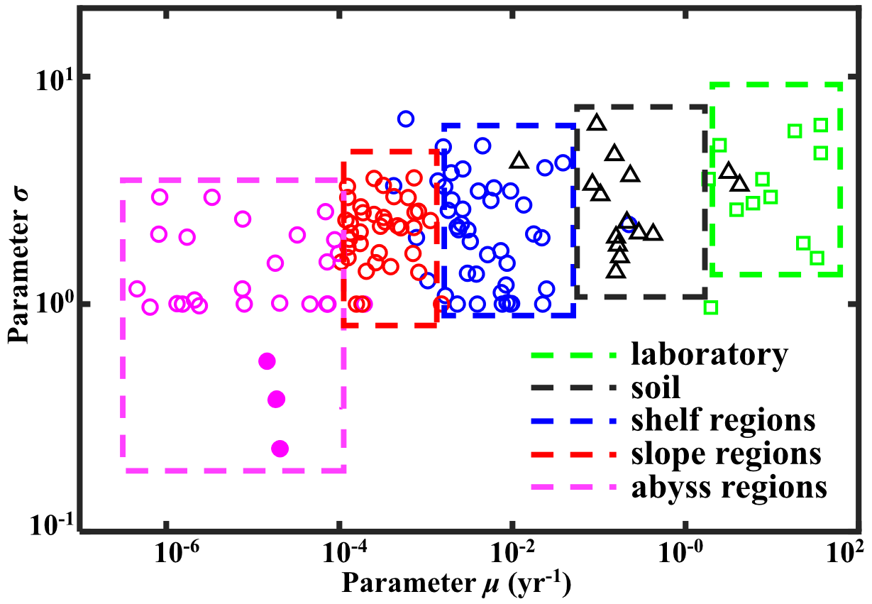
Figure 7 Regional distribution of OM reactivity. Distribution of parameters σ and μ in different regions. Solid pink circles denote fitting results of sites in the NEPAC with extremely low OM reactivity.

In addition to the difference between incubation data and field observations, Fig. 7 also reveals a decrease of 3 order of magnitude in inversely determined μ for OM from the shelf (10⁻³–10⁻¹ yr⁻¹) to the slope (10⁻⁴–10⁻³ yr⁻¹) and ultimately abyssal regions (< 10⁻⁴ yr⁻¹). In addition, shelf and slope regions also generally reveal a larger σ (1–3), while abyssal regions display a narrower σ range (0.5–1). This observed progressive decrease in μ and σ from the shelf to the abyssal ocean confirms previously observed patterns (Arndt et al., 2013; Freitas et al., 2021; Zonneveld et al., 2010) and reflects the interaction between OM structure (or its source) and the degree of alteration/pre-processing as OM transits from its original source to the ultimate sedimentary sink. In the dynamic shelf regions, highly variable OM loads from different sources – including in situ produced marine OM and laterally transported, pre-processed terrestrial or marine OM – are often physically protected from further erosion/deposition cycles due to high suspended sediment loads (Arndt et al., 2013; Larowe et al., 2020a). As a result, benthic OM is composed of a complex mixture of fresh and pre-aged compounds of highly variable (hence larger σ of the initial distribution) yet generally higher overall reactivity. On the upper and mid-continental slopes, intensive lateral or vertical transport processes or the abrupt relocation of sediment results in similar complex mixtures of OM (hence similar σ of the initial distribution) (Larowe et al., 2020a). However, transport timescales are often longer due to the greater water depths and distance to land. The deposited OM is generally more degraded and thus less reactive than in shelf environments. In contrast, benthic OM in abyssal regions is mainly derived from marine production (Rowe and Staresinic, 1979; Larowe et al., 2020a). During its slow settling through the water column, highly reactive OM compounds are rapidly degraded, and only the less reactive compounds persist and settle onto the sediment (Dunne et al., 2007). The values of μ and σ in the abyssal regions are thus significantly smaller than in the shelf and slope regions. The decrease in μ and σ from the shelf to abyssal regions reveals a decline in reactivity during lateral transport of OM, where μ mainly controls the overall reactivity and σ indicates the coverage of the main component of OM.

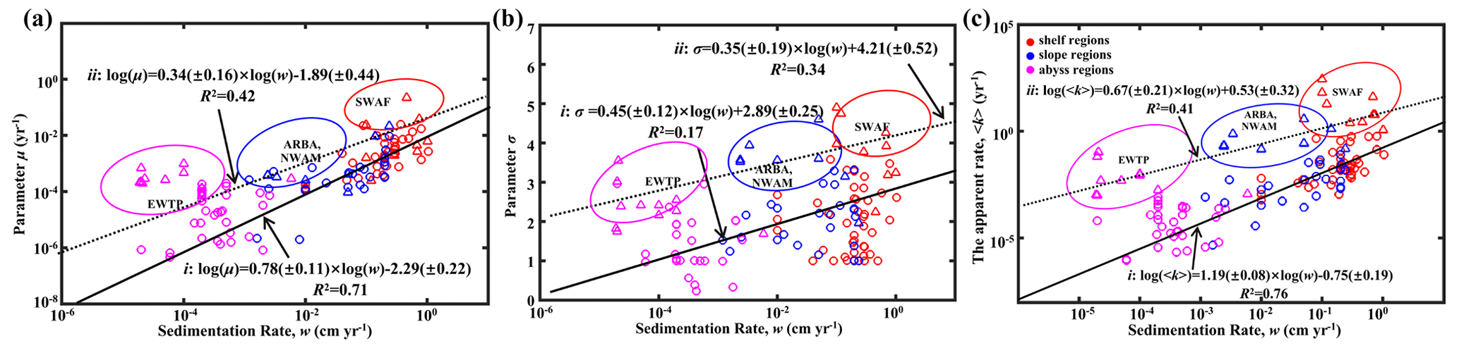
Figure 8 Global distribution patterns of OM reactivity. (a) Log–log plot of ω and μ. (b) Log–log plot of ω and σ. (c) Log–log plot of ω and 〈k〉. The solid black line (i) denotes linear regression for shelf, slope and abyssal regions. The dotted black line (ii) denotes linear regression for high OM reactivity regions, including the EWTP, ARBS, NWAM and SWAF regions.

Table 2 Abbreviations of regions in this paper (Seiter et al., 2004) and their area, mean water depth, mean OM content in surface sediment (< 5 cm) and apparent OM degradation rata (〈K_region〉).

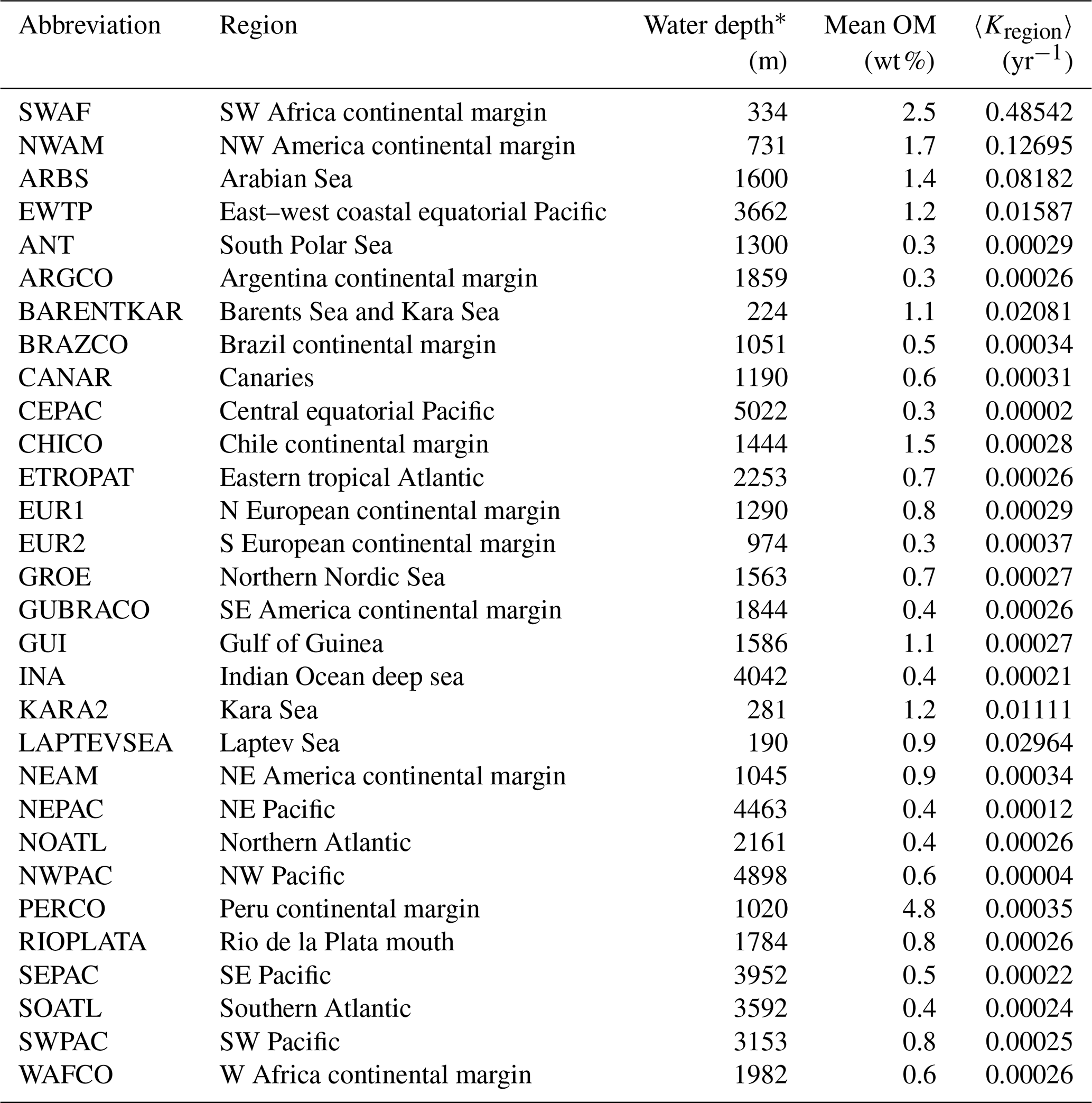
^∗ Water depth and mean OM content are based on the average depth and OM content of the sites in each region of Fig. 4.

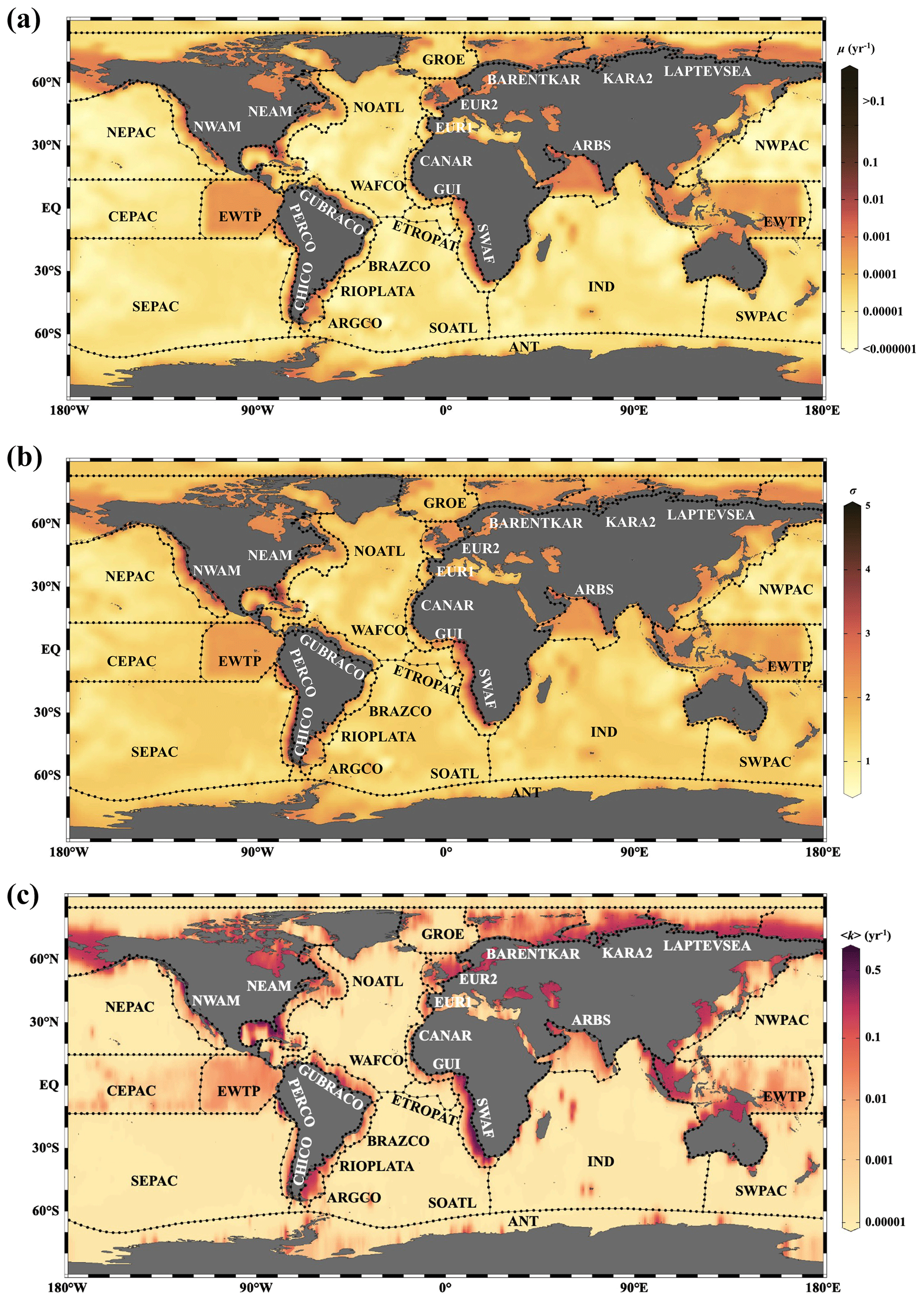
Figure 9 Distribution of μ (a), σ (b) and 〈k〉 (c) in the global ocean with 1^∘ × 1^∘ resolution.

3.3 Global distribution patterns of OM reactivity

Parameters μ and σ together control the degradation process of OM, which can be further described by the apparent degradation rate of the bulk OM (〈k〉). Sedimentation rate (ω) is a widely observed and comparably easy to measure proxy for local depositional conditions with sizable global datasets or empirical formulas available (Burwicz et al., 2011). Figure 8a–c show the global decreasing trend of μ, σ and 〈k〉 with ω for the general sea regions (shelf, < 200 m; slope, 200–2000 m; and abyss, > 2000 m). The active OM fractions (e.g., sugars and proteins) are preferentially exhausted during the lateral transport of OM from the shelf to the abyssal regions, leading to a decrease in the mean OM reactivity (μ; Fig. 8a), and thus OM is mainly composed of refractory components (σ; Fig. 8b). Due to the multiple sources of OM in the shelf regions, including fresh and older OM imported laterally by inland rivers, and OM settled from the euphotic layer (LaRowe et al., 2020a), the values of μ, σ and 〈k〉 fluctuate significantly. However, the general trend is superimposed by a large variability and apparent reactivity 〈k〉 in specific environments, notably deviating from this generally observed trend. More specifically, higher μ and σ values and, thus, higher OM reactivities occur in the eastern–western coastal equatorial Pacific (EWEP), southwestern Africa continental margin (SWAF), northwestern America continental margin (NWAM) and the Arabian Sea (ARBS) regions. These results are completely consistent with prior observations and model results (Arndt et al., 2013) and can be directly linked to the prevailing water-column redox and depositional conditions. High benthic OM reactivities have previously been reported for depositional environments that are characterized by a dominance of marine algal OM (Hammond et al., 1996) and strong lateral transport processes (e.g., SWAF, NWAM) (Arndt et al., 2013). Consequently, the larger values of all μ, σ and 〈k〉 occur in the inverse modeling results for these depositional environments (Fig. 8). Furthermore, the reactivity of sedimentary OM is considerably influenced by oxygen content or, more precisely, by oxygen exposure time in the water column and at the seafloor (Aller, 1994; Hartnett et al., 1998; Hedges and Keil, 1995; Mollenhauer et al., 2003; Zonneveld et al., 2010). Lower oxygen concentrations, as present in these regions in the form of pronounced oxygen minimum zones (OMZs), will slow down the degradation of OM both in the water column and at the sediment surface (Jørgensen et al., 2022). This enables the burial of more reactive OM into the sediments and thus results in the occurrence of high sedimentary OM reactivity in these regions despite great water depth (e.g., ARBS, EWTP) (Arndt et al., 2013; Bogus et al., 2012; Ingole et al., 2010; Luff et al., 2000; Volz et al., 2018). The l-RCM not only captures the broad patterns of OM reactivity across the global seafloor even better than previous models but also provides statistically more significant relationships between OM reactivity (〈k〉) and sedimentation rate (ω) than inversely determined parameters of the γ-RCM (R² < 0.46) and discrete models (R² < 0.1) (Arndt et al., 2013). Considering that no robust quantitative framework exists at this stage to predict OM reactivity as a function of easily observable environmental parameters, the l-RCM provides an excellent first-order predictor and a step forward in assessing the global distribution patterns of OM reactivity despite the poor relationship between 〈k〉 and ω for these special regions (e.g., EWEP, SWAF, NWAM and ARBS).

Based on the empirical relationships in Fig. 8 (i. for the general water depth-related regions and ii. for the specific regions – EWTP, ARBS, NWAM and SWAF) and the water depth–ω relationship (Eq. 8), we finally derived, to our knowledge, the world's first map of the global distribution of parameters μ, σ and 〈k〉 (Fig. 9). Using the relationship between water depth, ω and 〈k〉 (Figs. 3 and 8c), we further estimated the mean apparent OM reactivity (〈K_region〉) in the 30 regions of global ocean (Table 2). Furthermore, the heterogeneity of the OM reactivity distribution in global marine sediments is illustrated well in Fig. 9. Specifically, higher μ (Fig. 9a), σ (Fig. 9b) and OM reactivity (Fig. 9c) is reflected in shelf regions, particularly in northern Atlantic provinces with high latitudes (e.g., Barents Sea, 〈K_region〉 ≈ 0.02 yr⁻¹; Laptev Sea, 〈K_region〉 ≈ 0.03 yr⁻¹; and Kara Sea, 〈K_region〉 ≈ 0.01 yr⁻¹), due to shallower water depths and high OM fluxes from inland (Burwicz et al., 2011; Seiter et al., 2004). Besides that, the global map also highlights the extremely low OM reactivity, especially in some regions, as indicated by the absence of the sulfate–methane transition (SMT) (e.g., the NE Pacific, NEPAC) (Egger et al., 2018) and central ocean gyre regions (e.g., South Pacific gyre) (LaRowe et al., 2020b). Deeper water depth (> 5000 m), relatively low OM content (∼ 0.2 wt %) and the old OM age (> 10⁴ years) result in comparably lower μ and σ values (Fig. 9a and b) and, thus, extremely low benthic OM reactivity (〈K_region〉 ≈ 10⁻⁴ yr⁻¹) (Kallmeyer et al., 2012; Müller and Suess, 1979). Normally, greater water depth enhances oxygen exposure time for OM degradation and thereby reduces the reactivity of OM arriving at the seafloor, as reflected in the smaller μ values (Fig. 9a). In ocean areas characterized by pronounced OMZs, however, due to strong coastal upwelling or a high export rate of plankton-derived OM, the inhibition of OM degradation processes in the water column results in the preservation of heterogeneously mixed OM components (both active and refractory), as reflected in the larger σ values (Fig. 9b), leading to higher than expected OM reactivity in specific regions despite greater water depths (e.g., ARBS and EWTP: 〈K_region〉 ≈ 0.01 yr⁻¹) (Fig. 9c). Thus, the l-RCM provides a new framework not only for identifying the differences in OM reactivity between regions but also for assessing regional and global OM reactivity patterns using easily obtainable information (e.g., sedimentation).

OM reactivity exerts an important control on the relative significance of OM degradation pathways in marine sediments. In oxic environments, OM will be mainly respired aerobically and through denitrification, whereas deeper within the sediment, it will mainly be decomposed through anaerobic pathways such as sulfate reduction and methanogenesis (Regnier et al., 2011). Therefore, further work should be conducted to simulate the associated biogeochemical processes using the l-RCM to better quantify OM degradation and burial in marine sediments on regional or global scales.

4 Conclusions

Compared with previous OM degradation models, the l-RCM presented here not only fits OM depth-content profiles well but also better represents the distribution of OM reactivity by the parameters μ and σ. We use the l-RCM to inversely determine μ and σ at 123 sites across the global ocean, including shelf, slope and abyssal regions. Our results show that the apparent OM reactivity ($\langle k\rangle =\mathit{\mu }\cdot \exp ({\mathit{\sigma }}^{\mathrm{2}}/\mathrm{2})$) decreases with decreasing sedimentation rate (ω) and that OM reactivity is more than 3 orders of magnitude higher in shelf than in abyssal regions. Due to the complex depositional environments (e.g., oxygen minimum zones), OM reactivity is higher than predicted in some specific regions (e.g., the NWAM, SWAF, ARBS and EWTP), which was also captured by the l-RCM in these regions. Based on two empirical relationships of 〈k〉 with ω and ω with z, we obtained the global OM reactivity distribution patterns and finally mapped the global OM reactivity distribution.

The reactivity of OM serving as fuel for microbial activity in marine sediments firmly controls the degradation pathways and metabolism rates. Thus, the l-RCM has direct implications on the constraints for OM degradation and burial in marine sediments on regional or global scales.