the Creative Commons Attribution 4.0 License.
the Creative Commons Attribution 4.0 License.
 | 20 Jun 2023
Quantifying land carbon cycle feedbacks under negative CO2 emissions
V. Rachel Chimuka
Claude-Michel Nzotungicimpaye
Kirsten Zickfeld
Land and ocean carbon sinks play a major role in regulating atmospheric CO2 concentration and climate. However, their future efficiency depends on feedbacks in response to changes in atmospheric CO2 concentration and climate, namely the concentration–carbon and climate–carbon feedbacks. Since carbon dioxide removal (CDR) is a key mitigation measure in emission scenarios consistent with global temperature goals in the Paris Agreement, understanding carbon cycle feedbacks under negative CO2 emissions is essential. This study investigates land carbon cycle feedbacks under positive and negative CO2 emissions using an Earth system model of intermediate complexity (EMIC) driven with an idealized scenario of symmetric atmospheric CO2 concentration increase (ramp-up) and decrease (ramp-down), run in three modes. Our results show that the magnitudes of carbon cycle feedbacks are generally smaller in the atmospheric CO2 ramp-down phase than in the ramp-up phase, except for the ocean climate–carbon feedback, which is larger in the ramp-down phase. This is largely due to carbon cycle inertia: the carbon cycle response in the ramp-down phase is a combination of the committed response to the prior atmospheric CO2 increase and the response to decreasing atmospheric CO2. To isolate carbon cycle feedbacks under decreasing atmospheric CO2 and quantify these feedbacks more accurately, we propose a novel approach that uses zero emission simulations to quantify the committed carbon cycle response. We find that the magnitudes of the concentration–carbon and climate–carbon feedbacks under decreasing atmospheric CO2 are larger in our novel approach than in the standard approach. Accurately quantifying carbon cycle feedbacks in scenarios with negative emissions is essential for determining the effectiveness of carbon dioxide removal in drawing down atmospheric CO2 and mitigating warming.
- Article
(2822 KB) - Full-text XML
-
Supplement
(1200 KB) - BibTeX
- EndNote


Anthropogenic CO2 emissions have increased substantially since the preindustrial era, increasing the risk of “severe, pervasive, and irreversible impacts” to the Earth system (IPCC, 2022). In an effort to reduce greenhouse gas emissions, nations adopted the Paris Agreement, which stipulated that surface warming should be kept well below 2 ∘C above preindustrial levels and encouraged efforts to further limit it to 1.5 ∘C (UNFCCC, 2015). Carbon dioxide removal (CDR) is a key mitigation measure in emission scenarios that are consistent with these climate goals (Ciais et al., 2013; Fuss et al., 2014; Rogelj et al., 2018, 2019; IPCC, 2022).
The land and ocean carbon sinks play a major role in regulating atmospheric CO2 concentration by absorbing approximately half of current anthropogenic CO2 emissions (Friedlingstein et al., 2022). However, this rate of absorption is sensitive to changes in climate and atmospheric CO2 concentration (Cox et al., 2000; Boer and Arora, 2010, 2013; Arora et al., 2013, 2020). As atmospheric CO2 concentration increases, carbon sinks will take up more carbon through air–sea exchange and CO2 fertilization, resulting in a negative concentration–carbon cycle feedback (Boer and Arora, 2010; Arora et al., 2013; Schwinger and Tjiputra, 2018). Conversely, changing climate, in response to the increasing CO2 concentration, will decrease the ability of carbon sinks to take up carbon, resulting in a positive climate–carbon cycle feedback (Cox et al., 2000; Jones et al., 2003; Fung et al., 2005; Friedlingstein et al., 2006; Boer and Arora, 2010, 2013; Zickfeld et al., 2011; Friedlingstein et al., 2014; Schwinger and Tjiputra, 2018).
Since the dominant feedback controlling land and ocean carbon uptake is the negative concentration–carbon feedback, the land and ocean are currently carbon sinks (Arora et al., 2020). However, the implementation of negative emissions is expected to weaken or even reverse natural carbon sinks. If negative emissions are implemented but remain lower than positive emissions (net-positive emissions), the land and ocean carbon sinks continue to take up carbon, albeit at a lower rate (Tokarska and Zickfeld, 2015; Jones et al., 2016; Melnikova et al., 2021; Koven et al., 2022). On land, the rate of carbon uptake declines because ecosystem respiration increases more than gross primary productivity increases, whereas, in the ocean, the rate of uptake declines following the declining CO2 emissions growth rate (Melnikova et al., 2021). Once the amount of CO2 removed from the atmosphere exceeds the amount of CO2 added to the atmosphere (net-negative emissions), the carbon sinks are expected to weaken further and may reverse (Cao and Caldeira, 2010; Tokarska and Zickfeld, 2015; Jones et al., 2016; Melnikova et al., 2021; Canadell et al., 2022; Koven et al., 2022). Decreasing CO2 levels will weaken the CO2 fertilization effect, decreasing net primary productivity (NPP) more than soil respiration, resulting in a flux of carbon into the atmosphere (Cao and Caldeira, 2010; Tokarska and Zickfeld, 2015). Furthermore, the gradient in the partial pressure of CO2 at the atmosphere–ocean interface will weaken and eventually reverse, resulting in the outgassing of CO2 (Cao and Caldeira, 2010; Tokarska and Zickfeld, 2015). Carbon losses from the land and ocean following CDR are expected to significantly decrease the effectiveness of CDR in drawing down atmospheric CO2 (Tokarska and Zickfeld, 2015; Jones et al., 2016; Zickfeld et al., 2021).
The behaviour of land carbon cycle feedbacks under positive and negative emissions is shown qualitatively in Fig. 1. As the atmospheric CO2 concentration increases under positive emissions, the land sequesters more carbon, reducing the atmospheric CO2 concentration (Boer and Arora, 2010; Arora et al., 2013). However, under negative emissions, the declining atmospheric CO2 concentration weakens and eventually reverses the land carbon sink, returning CO2 to the atmosphere. The concentration–carbon feedback is negative because it promotes carbon sequestration under positive emissions and drives carbon loss under negative emissions. As the climate warms under positive emissions, the land loses carbon to the atmosphere, increasing the atmospheric CO2 and causing further warming (Cox et al., 2000; Jones et al., 2003; Fung et al., 2005; Friedlingstein et al., 2006; Boer and Arora, 2010, 2013; Zickfeld et al., 2011; Friedlingstein et al., 2014). With cooling, the land carbon source weakens and eventually turns into a carbon sink, sequestering carbon and further cooling the climate under negative emissions. This positive climate–carbon feedback acts to amplify warming under positive emissions and enhance cooling under negative emissions.
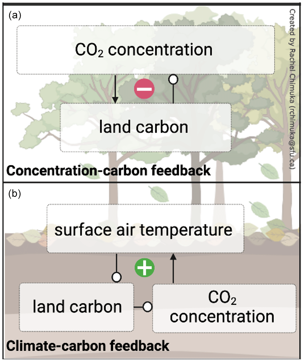
Figure 1Carbon cycle feedback schematic illustrating the behaviour of the (a) negative concentration–carbon feedback and (b) positive climate–carbon feedback. Each feedback loop starts with an increase (under positive emissions) or decrease (under negative emissions) in atmospheric CO2 concentration or surface air temperature. Arrows indicate a positive coupling (change in the same direction) between components and lines with empty circles indicate a negative coupling (change in the opposite direction) between components.
The goal of this study is to quantify land carbon cycle feedbacks under negative emissions. We address two research questions: (1) how does the magnitude of carbon cycle feedbacks under negative emissions compare to that under positive emissions? (2) Is the approach currently used to quantify carbon cycle feedbacks under positive emissions adequate to quantify feedbacks under negative emissions? If not, how can this approach be improved upon? This study investigates carbon cycle feedbacks under positive and negative emissions in an Earth system model of intermediate complexity (EMIC) driven with an idealized scenario of a 1 % yr−1 increase and decrease in atmospheric CO2 concentration. Our study adds to the small but growing body of research on carbon cycle feedbacks under negative emissions (Schwinger and Tjiputra, 2018; Melnikova et al., 2021) by exploring the behaviour of these feedbacks, with a focus on land processes. We propose a novel approach for quantifying carbon cycle feedbacks under negative emissions and provide insight into the role of these feedbacks in determining the effectiveness of carbon dioxide removal in reducing CO2 levels.
2.1 Model description
The University of Victoria Earth System Climate Model (UVic ESCM, version 2.10) (Fig. 2) is a model of intermediate complexity with a horizontal grid resolution of 1.8 ∘ (meridional) × 3.6 ∘ (zonal) (Weaver et al., 2001; Mengis et al., 2020). The model consists of a simplified atmospheric model, a 3D ocean general circulation model, including ocean inorganic and organic carbon cycle models, coupled to a dynamic–thermodynamic sea ice model, and a land surface model coupled to a vegetation model (including permafrost) (Mengis et al., 2020). The atmosphere is a 2D energy–moisture balance model with dynamical wind feedbacks. Atmospheric heat and freshwater are transported through diffusion and advection (Weaver et al., 2001), based on wind velocities prescribed from monthly climatological wind fields from NCAR/NCEP reanalysis data (Eby et al., 2013). The 19-layer 3D ocean general circulation model is based on the Geophysical Fluid Dynamics Laboratory (GFDL) Modular Ocean Model version 2 (MOM2; Pacanowski, 1995). The coupled dynamic–thermodynamic sea ice model simulates sea ice dynamics through elastic, viscous, and plastic deformation and flow mechanisms (Weaver et al., 2001). Ocean carbon is represented by an inorganic ocean carbon model following the Ocean Carbon Model Intercomparison Protocol (OCMIP), and an NPZD (nutrient, phytoplankton, zooplankton, detritus) model of ocean biology simulating carbon uptake by the biological pump, accounting for phytoplankton light and iron limitations (Keller er al., 2012). The land surface model, based on the Hadley Centre Met Office Surface Exchange Scheme (MOSES), simulates the terrestrial carbon cycle and is coupled to the Top-Down Representation of Interactive Foliage and Flora including Dynamics (TRIFFID) model which simulates vegetation and soil carbon (Meissner et al., 2003). This model version also includes a permafrost carbon model in the soil module that simulates permafrost carbon through a diffusion-based scheme (MacDougall and Knutti, 2016).
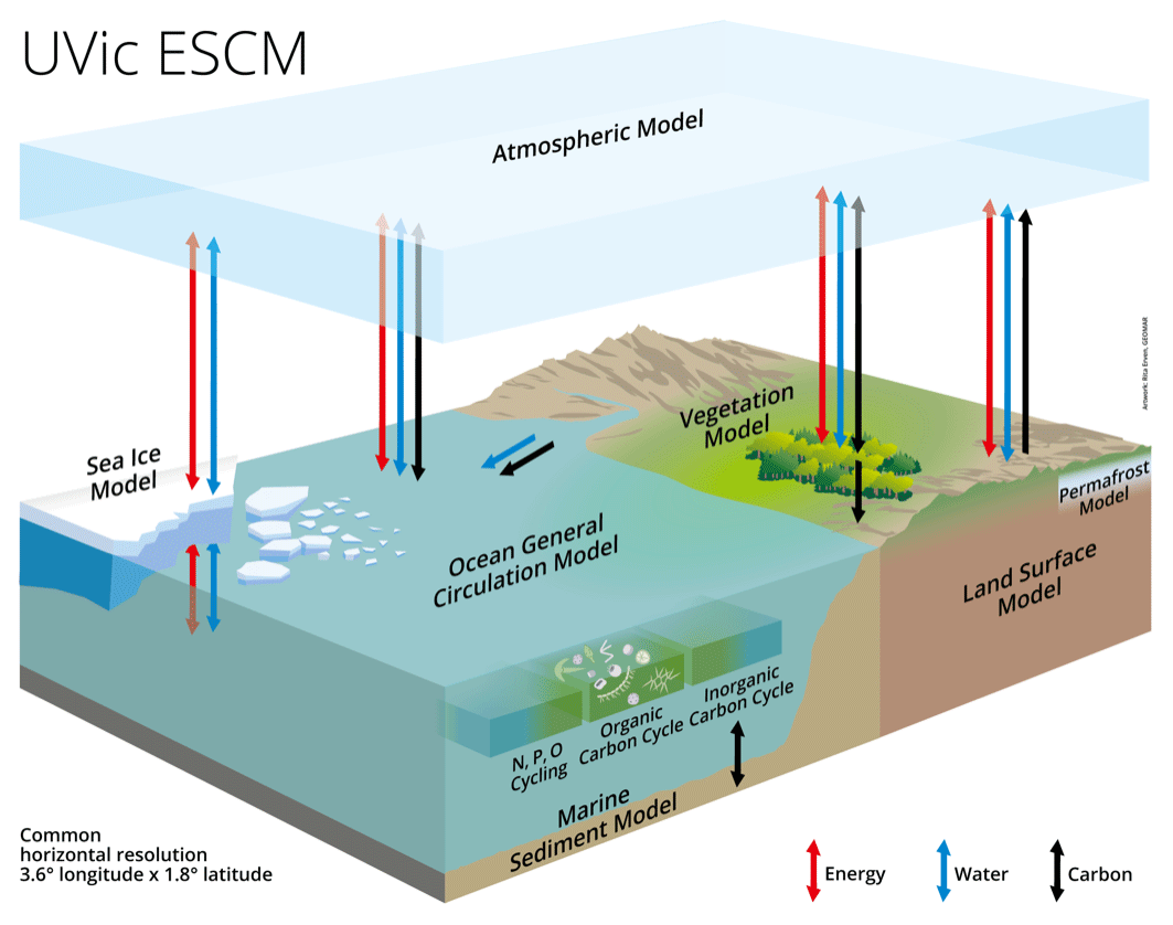
Figure 2University of Victoria Earth System Climate Model (UVic ESCM) schematic. Energy, water, and carbon exchanges between model components are represented by arrows. Figure reproduced with permission from Mengis et al. (2020).
2.2 Model simulations
We performed a preindustrial spin-up simulation to equilibrate the model with the preindustrial CO2 concentration (∼285 ppm). All other greenhouse gas concentrations, surface land conditions, and orbital parameters were held at 1850 levels according to the Coupled Model Intercomparison Project Phase 6 (CMIP6) experimental design protocol (Eyring et al., 2016). The solar forcing was set to the 1850–1873 mean and the volcanic forcing was held at its average over 1850–2014, also consistent with the CMIP6 protocol (Eyring et al., 2016).
To explore how the magnitude of carbon cycle feedbacks under positive emissions differs from that under negative emissions, we ran the “CDR-reversibility” simulation from the Carbon Dioxide Removal Model Intercomparison Project (CDRMIP; Keller et al., 2018). Starting from a preindustrial equilibrium state, atmospheric CO2 concentration was prescribed to increase at 1 % yr−1 until quadrupling, then decline back to preindustrial levels at the same rate. Achieving such a rapid decline in CO2 concentration would only be possible with substantial negative CO2 emissions (Boucher et al., 2012). We refer to the section of the prescribed CO2 concentration trajectory with increasing CO2 concentration as the ramp-up phase and the section with decreasing CO2 concentration as the ramp-down phase.
We also ran a zero emission simulation (“Zeroemit”) for use in our novel approach for quantifying the “committed” carbon cycle response to increasing atmospheric CO2 during the ramp-up phase. This simulation was initialized from the peak atmospheric CO2 concentration in the CDR-reversibility simulation and run in emission-driven configuration. Emissions were set to zero at the start of the simulation, then CO2 was allowed to evolve for 500 years.
The CDR-reversibility and Zeroemit simulations were run in three modes, following the C4MIP protocol for the quantification of carbon cycle feedbacks (Friedlingstein et al., 2006; Arora et al., 2013, 2020; Jones et al., 2016).
Fully coupled mode (FULL): the entire Earth system responds to the specified change in atmospheric CO2 concentration or CO2 emissions – in this mode, the land and ocean carbon sinks are subject to changing atmospheric CO2 concentration and temperature.
Biogeochemically coupled mode (BGC): the land and ocean carbon sinks are subject to changing atmospheric CO2 concentration but not changing temperature – this is achieved by prescribing a specified time-invariant CO2 concentration to the radiation module (preindustrial CO2 concentration for the CDR-reversibility simulation and quadruple the preindustrial CO2 concentration for the Zeroemit simulation), while the land and ocean carbon cycle modules see an evolving atmospheric CO2 concentration.
Radiatively coupled mode (RAD): the land and ocean carbon sinks are subject to changes in temperature but no change in atmospheric CO2 concentration – the land and ocean carbon cycle modules see a specified time invariant CO2 concentration (preindustrial CO2 concentration in the CDR-reversibility simulation and quadruple the preindustrial CO2 concentration in the Zeroemit simulation), while the radiation module sees changing atmospheric CO2 concentration.
In both the CDR-reversibility and Zeroemit simulations, non-CO2 forcings are held fixed at their preindustrial values.
2.3 Approaches to carbon cycle feedback quantification
In the first approach (referred to as the “standard” approach), we use the CDR-reversibility simulation to quantify carbon cycle feedbacks under increasing and decreasing atmospheric CO2 concentration. Although this simulation is highly idealized, the ramp-up phase is standardly used to quantify carbon cycle feedbacks under positive emissions, and therefore, allows easier comparison of these results to other literature. The ramp-up phase represents the response to increasing atmospheric CO2 alone. However, the ramp-down phase represents the response to both the prior increasing CO2 and decreasing CO2 because the latter is prescribed when the system is still in a transient (that is, time-evolving) state, responding to the prior atmospheric CO2 increase (Zickfeld et al., 2016; Keller et al., 2018). As a result, carbon cycle feedbacks quantified from the ramp-down phase do not represent the response to decreasing atmospheric CO2 alone.
Our second and novel approach, therefore, aims to improve the quantification of carbon cycle feedbacks under decreasing CO2 by isolating the carbon cycle response to decreasing CO2 alone. We use an experimental design utilizing both the CDR-reversibility and Zeroemit simulations. Since the Zeroemit simulation quantifies the committed or lagged response to the prior positive emissions, the first 140 years of this simulation was subtracted from the ramp-down phase of the CDR-reversibility simulation to isolate the response to decreasing CO2 alone. A similar approach was used in Zickfeld et al. (2016) to quantify the temperature response to decreasing atmospheric CO2. The main assumption made here is that of linearity: that is, we assume that the committed carbon cycle response to the prior CO2 increase and the carbon cycle response to the CO2 decrease combine linearly to the total carbon cycle response in the ramp-down phase. From our approach – referred to as the “inertia-corrected” approach – we quantify carbon cycle feedbacks and compare them to those from the first approach.
2.4 Carbon cycle feedback metrics
We use integrated flux-based feedback parameters (Friedlingstein et al., 2006) to quantify carbon cycle feedbacks in both approaches. In this framework, changes in land and ocean carbon are expressed as the sum of two terms: a term representing the change in land (ocean) carbon in response to changes in atmospheric CO2, and a term representing the change in land (ocean) carbon in response to changes in surface air temperature:
where the subscript X represents land or ocean. The concentration–carbon feedback parameter β quantifies the carbon cycle response to changes in CO2 concentration in units of petagrams of carbon per part per million (PgC ppm−1), whereas the climate–carbon feedback parameter γ quantifies the carbon cycle response to changes in climate in units of petagrams of carbon per degree Celsius (PgC ∘C−1).
The change in land (ocean) carbon due to changing atmospheric CO2 concentration is determined using the biogeochemically coupled (BGC) simulation. In this simulation, the land and ocean only respond to changes in the CO2 concentration, and therefore, this simulation can be used to quantify the concentration–carbon feedback parameter β. Warming is still observed in these simulations because the water use efficiency of vegetation increases at higher CO2 concentrations and changes in albedo due to shifts in vegetation structure and spatial distribution, resulting in a small warming effect (Cox et al., 2004, Boer and Arora, 2013; Arora et al., 2013). However, this warming is considered negligible in this framework (Friedlingstein et al., 2006). Assuming that ΔT=0 in Eq. (1), the change in land (ocean) carbon due to changes in atmospheric CO2 concentration is expressed as follows:
Equation (2) can then be rearranged to solve for the concentration–carbon feedback parameter β as follows:
The change in land (ocean) carbon due to climate change is determined using the radiatively coupled (RAD) simulation. In this simulation, the land and ocean only respond to changes in climate, and therefore, this simulation can be used to quantify the climate–carbon feedback parameter γ. The change in land (ocean) carbon due to climate change is expressed as
Equation (4) can then be rearranged to solve for the climate–carbon feedback parameter γ as follows:
An alternative method for quantifying the change in land (ocean) carbon due to climate change uses the fully coupled and biogeochemically coupled simulations (Arora et al., 2013). Here, we refer to this method as the FULL–BGC method. Here, the change in land (ocean) carbon in the biogeochemically coupled simulation (BGC) is subtracted from that in the fully coupled simulation (FULL) and expressed as the product of the climate–carbon feedback parameter, and the difference between the surface air temperature changes in the two simulations:
Equation (6) can then be rearranged to solve for the climate–carbon feedback parameter γ as follows:
The resulting feedback parameters differ from those quantified from the RAD mode (Eq. 5) alone due to nonlinearities in carbon cycle feedbacks (Zickfeld et al., 2011; Schwinger et al., 2014).
Feedback parameters under increasing atmospheric CO2 (ramp-up phase) are computed at the peak atmospheric CO2 concentration (quadruple the preindustrial level) using changes in carbon pools, atmospheric CO2 concentration, and surface air temperature computed relative to preindustrial levels. Feedback parameters under decreasing atmospheric CO2 (ramp-down phase) are computed at the return to preindustrial levels (end of ramp-down phase) using changes in carbon pools, atmospheric CO2 concentration, and surface air temperature computed relative to the time of peak atmospheric CO2.
In the ramp-up phase, feedback parameters are positive for land or ocean carbon gain and negative for land or ocean carbon loss. Note that the signs we refer to here are not the signs of the feedback but rather the signs of the feedback parameters, which are generally opposite to the sign of the feedback because they are computed from the perspective of the land and ocean, whereas the sign of the feedback is determined from the perspective of the atmosphere. In the ramp-down phase, both atmospheric CO2 concentration and surface air temperature decline relative to their values at the end of the ramp-up phase, resulting in a negative denominator (see Eqs. 3, 5, 7). Therefore, the sign convention is reversed: feedback parameters are negative for a gain in land or ocean carbon (positive numerator divided by negative denominator) and positive for a loss in land or ocean carbon (negative numerator divided by negative denominator).
2.4.1 Isolating carbon cycle feedbacks under negative emissions
When a CO2 decrease is prescribed from a transient state, the land and ocean carbon pools not only respond to this CO2 decrease but also to the prior CO2 trajectory due to inertia in these systems (Zickfeld et al., 2016). The land (ocean) carbon cycle responses in the ramp-down phase can, therefore, be expressed as the sum of two terms: one term driven by the sensitivities of land (ocean) to the CO2 and temperature decrease during the ramp-down phase (“SENS” for sensitivity) and an inertia term that represents the lagged response to past atmospheric CO2 and climate changes (“LAG”):
The carbon pool response to the CO2 and temperature decrease can then be isolated as follows:
where is driven by the sensitivities to changes in atmospheric CO2 (β) and temperature (γ) in the ramp-down phase and can be linearly decomposed in the same way as the land and ocean carbon response in the standard framework (Eq. 1):
Here, ΔCA and ΔT refer to the changes in atmospheric CO2 and temperature in the ramp-down phase of the CDR-reversibility simulation relative to their values at the end of the ramp-up phase. This framework becomes identical to the standard framework (Sect. 2.4) in cases where a change in atmospheric CO2 is applied from a state of equilibrium, i.e. .
Equation (10) can be rewritten for the biogeochemically (ΔT=0) and radiatively coupled simulations (ΔCA=0), respectively:
Rearranging the equations above allows for the calculation of the feedback parameters, which measure the sensitivity of the land and ocean carbon responses to changes in CO2 concentration and temperature in the ramp-down phase:
The lagged responses of land and ocean carbon pools are calculated from the Zeroemit simulations run in the respective mode (biogeochemically coupled for the calculation of β and radiatively coupled for the calculation of γ), and they are then subtracted from the responses of the ramp-down phase of the CDR-reversibility simulations run in the same mode. The land (ocean) carbon changes, surface air temperature, and CO2 concentration changes are computed relative to the year of peak CO2 concentration (year 140 in the CDR-reversibility simulation; year 1 in the zero emission simulation).
3.1 CDR-reversibility carbon cycle feedback analysis
Our results focus on the ramp-down phase of the CDR-reversibility simulation and compare the system response in this phase to that in the ramp-up phase. While the prescribed atmospheric CO2 concentration for the CDR-reversibility simulations is the same, the temperature response differs by mode (Fig. 3a, b). In the FULL and RAD modes, surface air temperature increases approximately linearly with increasing atmospheric CO2 concentration, continues to increase for approximately half a decade after atmospheric CO2 concentration peaks, then decreases with decreasing CO2 concentration. Surface air temperature declines more slowly in the ramp-down phase due to the thermal inertia of the ocean, and therefore, does not return to preindustrial levels by the end of the ramp-down phase. The temperature response in the FULL mode is consistent with earlier studies (Boucher et al., 2012; Zickfeld et al., 2016; MacDougall, 2019; Ziehn et al., 2020; Park and Kug, 2022). Surface air temperature in the BGC mode changes only marginally: surface air temperature increases slightly with increasing CO2 concentration and decreases as the CO2 concentration decreases. This temperature change is driven by biophysical responses to changing atmospheric CO2, in particular, changes in evaporative fluxes as plants adjust stomatal conductance based on atmospheric CO2 levels. Biophysical effects are also responsible for the difference in warming between the FULL and RAD modes (Arora et al., 2020). The temperature response in the ramp-up phase of the FULL, BGC, and RAD modes is consistent with Arora et al. (2020), while the temperature response in the ramp-up and ramp-down phases of all three modes is consistent with Schwinger and Tjiputra (2018).
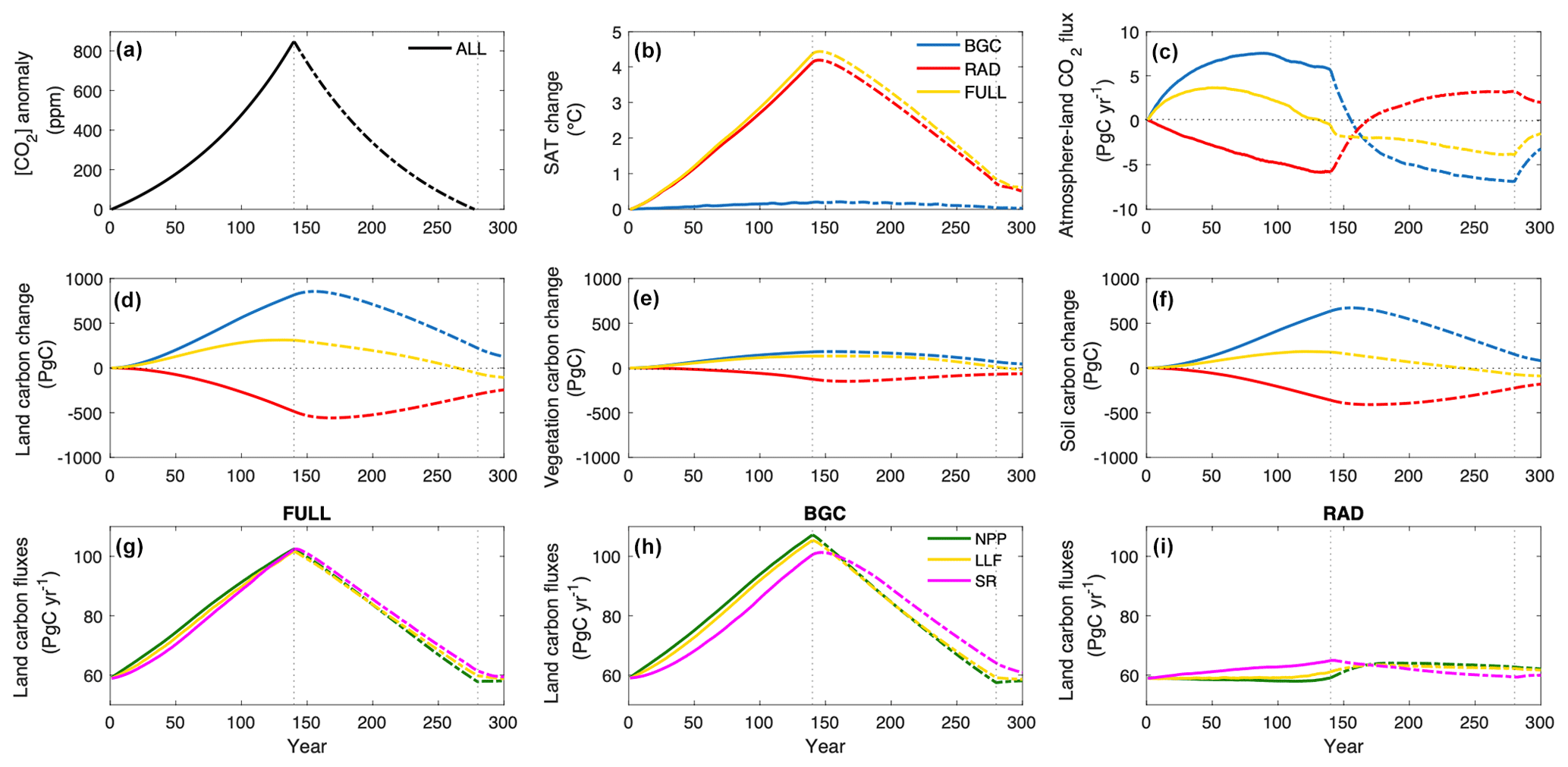
Figure 3(a) Prescribed atmospheric CO2 concentration anomaly; (b) surface air temperature (SAT) change; (c) atmosphere-to-land CO2 flux; and (d) land, (e) vegetation, and (f) soil carbon pool changes in the fully coupled (FULL), biogeochemically coupled (BGC), and radiatively coupled (RAD) CDR-reversibility simulations. Panels (a), (b), and (d–f) are calculated relative to 1850 (preindustrial). Carbon fluxes for the three modes are shown in the bottom row (g, h, i): NPP: net primary productivity, LLF: leaf litter flux, and SR: soil respiration. Solid lines represent the ramp-up phase and dot-dashed lines represent the ramp-down phase. The vertical dotted lines mark the beginning and end of the ramp-down phase.
3.1.1 Land carbon change in the FULL mode
Figure 3d shows land carbon pool changes as a function of time. In the FULL mode, land carbon increases, stabilizes, then begins to decrease 7 years before the peak atmospheric CO2 concentration is reached. Similar carbon pool change patterns are observed for the soil carbon pool, which starts decreasing roughly 20 years before the peak in atmospheric CO2 concentration, but vegetation carbon decreases 2 years after the peak atmospheric CO2 concentration (Fig. 3e, f). Our results are qualitatively consistent with Ziehn et al. (2020). However, they differ from other studies (MacDougall, 2019; Arora et al., 2020) wherein the land carbon pool remains a carbon sink in the ramp-up phase. MacDougall (2019) shows that the soil carbon sink switches into a source later in the ramp-up phase than our results show. Furthermore, other studies (Boucher et al., 2012; Zickfeld et al., 2016) show that both vegetation and soil carbon sinks persist throughout the ramp-up phase.
Here, land carbon decreases throughout the ramp-down phase (Fig. 3d), whereas earlier studies show continued increase in the land carbon pool in the early ramp-down phase (Boucher et al., 2012; Zickfeld et al., 2016; Park and Kug, 2021). Changes in land carbon are governed by the balance between net primary productivity (NPP) and soil respiration. The increase in the land carbon pool is driven by the CO2 fertilization effect: photosynthesis is enhanced under increasing CO2 concentration, increasing NPP (Fig. 3g) (Arora et al., 2013). Soil respiration also increases with warming (Fig. 3g). Initially, soil respiration remains below NPP, but the rate of increase of NPP declines faster and soil respiration exceeds NPP towards the end of the ramp-up phase. This occurs due to the different response timescales of NPP and soil respiration: NPP depends on atmospheric CO2 changes, whereas soil respiration depends on temperature change, which lags behind the change in CO2 concentration (Cao and Caldeira, 2010). In the ramp-down phase, NPP decreases as the CO2 fertilization effect weakens, whereas soil respiration continues to increase for a year before decreasing at a slower rate than NPP, driven by decreasing surface air temperature and soil carbon.
3.1.2 Land carbon change in the BGC mode
In the BGC mode, land carbon increases in the ramp-up phase, continues to increase until 16 years after the peak in CO2 concentration, then decreases (Fig. 3d). A similar lag is observed for both vegetation and soil carbon pools, but the soil carbon sink persists for 5 years longer than the vegetation carbon sink (Fig. 3e, f). Land carbon increases in the ramp-up phase due to the CO2 fertilization effect, which increases NPP (Fig. 3h) (Arora et al., 2013). In the UVic ESCM, soil respiration depends on soil temperature, moisture, and carbon content (Cox et al., 2001; Mengis et al., 2020). Since changes in surface air temperature in the BGC mode are small (Fig. 3b), changes in the first two factors are negligible and soil carbon content is the main driver of soil respiration changes. Soil respiration increases with increasing soil carbon, but NPP remains higher, resulting in an increase in the land carbon pool in the ramp-up phase (Fig. 3h). In the ramp-down phase, NPP decreases as the CO2 fertilization effect weakens, whereas soil respiration continues to increase before decreasing at a slower rate than NPP, following changes in soil carbon (Fig. 3h). Net primary productivity (NPP) declines below soil respiration, and land carbon begins to decrease.
3.1.3 Land carbon change in the RAD mode
Land carbon decreases in the ramp-up phase of the RAD mode, continues to decrease until roughly 30 years after the peak in atmospheric CO2 concentration, then switches into a carbon sink (Fig. 3d). Both vegetation and soil carbon pools exhibit a similar lag, but the vegetation carbon pool remains a carbon source for a decade longer than the soil carbon pool (Fig. 3e, f). Land carbon decreases in the ramp-up phase because NPP decreases as plant respiration rates increase (see Fig. S1 in the Supplement), whereas soil respiration increases with warming (Fig. 3i), consistent with earlier literature (Arora et al., 2020). The NPP later increases due to vegetation shifts that occur on decadal to centennial timescales (see Fig. S2) but remains lower than soil respiration. In the ramp-down phase, NPP increases (Fig. 3i) as gross primary productivity increases and plant respiration decreases with cooling, then later declines as gross primary productivity declines, because cooler temperatures negatively impact vegetation growth in the high latitudes (see Figs. S1, S3). Soil respiration decreases steadily with declining surface air temperature, and after a few decades, declines below NPP, and the land carbon pool begins to grow again.
3.1.4 Ocean carbon change in the FULL, BGC, and RAD modes
In the FULL mode, the ocean carbon pool grows at a steady rate, then begins to slowly lose carbon roughly three decades after the peak in atmospheric CO2 concentration (Fig. 4a). In the ramp-up phase, the partial pressure of CO2 in the atmosphere increases, strengthening the partial pressure gradient and driving an influx of CO2 into the ocean (Fig. 4b). In the ramp-down phase, the gradient in partial pressure weakens and eventually reverses, and the ocean carbon sink switches into a source. Earlier studies forced with the CDR-reversibility simulation also show ocean carbon uptake in the ramp-up phase (MacDougall, 2019; Arora et al., 2020) followed by delayed carbon loss in the ramp-down phase (Boucher et al., 2012; Zickfeld et al., 2016).
The ocean exhibits a delayed response in the ramp-down phase of the BGC and RAD modes consistent with Schwinger and Tjiputra (2018). In the BGC mode, ocean carbon increases in the ramp-up phase, continues to increase for approximately half a century after the peak atmospheric CO2 concentration, then switches into a source of carbon (Fig. 4a). The partial pressure gradient of CO2 strengthens in the ramp-up phase, driving CO2 uptake, then weakens and reverses in the ramp-down phase, promoting carbon loss, but the magnitude of the flux is larger than in the FULL mode (Fig. 4b). In the RAD mode, ocean carbon decreases in the ramp-up phase, continues to decrease for over a century in the ramp-down phase, then switches into a weak carbon sink (Fig. 4a). The ocean outgasses in the ramp-up phase, possibly due to climate effects on ocean circulation and the solubility pump (Cox et al., 2000; Fung et al., 2005; Friedlingstein et al., 2006; Zickfeld et al., 2011). In the ramp-down phase, the ocean remains a carbon source for over a century before switching into a weak carbon sink. Ocean carbon changes in the BGC and RAD modes are also driven by the concentration–carbon and climate–carbon feedbacks. An in-depth discussion of the mechanisms behind the ocean carbon response is beyond the scope of this paper.
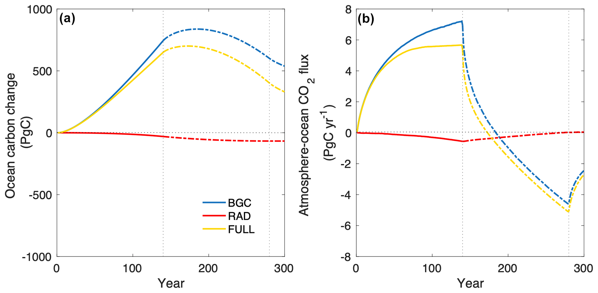
Figure 4(a) Ocean carbon change and (b) atmosphere-to-ocean CO2 flux in the fully coupled (FULL), biogeochemically coupled (BGC), and radiatively coupled (RAD) CDR-reversibility simulations. Ocean carbon change is calculated relative to 1850 (preindustrial). Solid lines represent the ramp-up phase and dot-dashed lines represent the ramp-down phase. The vertical dotted lines mark the beginning and end of the ramp-down phase.
3.1.5 Sensitivity of land and ocean carbon pools
To assess the sensitivity of land and ocean carbon pools to changes in atmospheric CO2 and temperature, we plot carbon changes in the BGC mode as a function of atmospheric CO2 concentration (Fig. 5) and carbon changes in the RAD mode as a function of surface air temperature (Fig. 6). The trajectory of carbon change differs in the ramp-up and ramp-down phases of the BGC mode (Fig. 5), a behaviour referred to as hysteresis. Hysteresis in the land carbon pool is primarily driven by the soil carbon pool, although the contribution from the vegetation carbon pool is also significant (Fig. 5a, c, d). The width of the hysteresis – measured as the vertical distance between the ramp-up and ramp-down trajectories – initially increases, then decreases (Fig. 5a–d), except in the vegetation carbon pool where the width of the hysteresis increases throughout the ramp-down phase (Fig. 5c). The land and ocean carbon pools in the RAD mode also exhibit hysteresis (Fig. 6). The hysteresis in the land carbon pool is dominated by the soil carbon pool (Fig. 5d), and the width of the hysteresis appears to increase throughout the ramp-down phase for all carbon pools except the vegetation carbon, which shows nearly constant hysteresis. The observed hysteresis in the land and ocean carbon pools in the BGC and RAD modes is likely largely due to climate system inertia: the carbon cycle response in the ramp-down phase is a combination of the response to both increasing and decreasing CO2 concentrations.
Despite the restoration of preindustrial atmospheric CO2 levels in the BGC mode, the land and ocean carbon pools do not return to their preindustrial states. At the end of the ramp-down phase, the land carbon pool holds approximately 250 PgC more than at the preindustrial state, with 80 PgC remaining in the vegetation carbon pool and 170 PgC remaining in the soil carbon pool (Fig. 5a, c, d) due to time lags associated with vegetation and soil carbon turnover. The ocean carbon pool holds much more carbon (615 PgC) than at the preindustrial state (Fig. 5b). In the RAD mode, the land and ocean carbon lost in the ramp-up phase is not completely regained in the ramp-down phase, though this response would be expected, given the asymmetric surface air temperature response in this mode. By the end of the RAD mode, the land carbon pool holds approximately 300 PgC less than at the preindustrial state, with the vegetation carbon pool accounting for 70 PgC and the soil carbon pool accounting for the remaining 230 PgC (Fig. 6a, c, d). The ocean holds only 70 PgC less than at the preindustrial state, but unlike the land carbon pool, a minuscule amount of ocean carbon is regained in the ramp-down phase (Fig. 6b).
Previous studies have shown carbon cycle hysteresis in the FULL mode of the CDR-reversibility simulation (Boucher et al., 2012; Zickfeld et al., 2016; Jeltsch-Thömmes et al., 2020; Park and Kug, 2022), consistent with our results (see Fig. S4). However, in most of these studies, the vegetation and soil carbon pools do not return to their preindustrial states by the end of the ramp-down phase (Boucher et al., 2012; Zickfeld et al., 2016; Park and Kug, 2022). Our results for the FULL mode of the CDR-reversibility simulation show that the vegetation and soil carbon pools are very close to their preindustrial states by the end of the ramp-down phase (see Fig. S4), consistent with Ziehn et al. (2020), who show a near-return to the preindustrial state in the vegetation carbon pool.
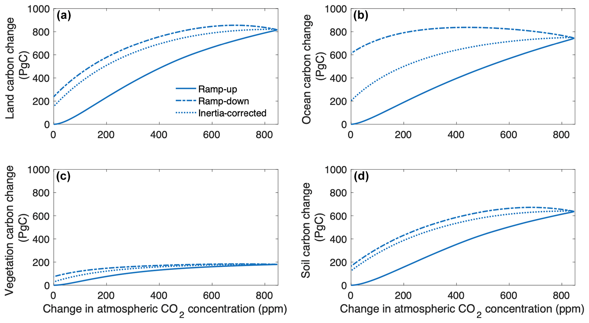
Figure 5(a) Land, (b) ocean, (c) vegetation, and (d) soil carbon pool changes as a function of atmospheric CO2 concentration, taken from the biogeochemically coupled (BGC) CDR-reversibility simulation ramp-up and ramp-down phases and the inertia-corrected approach. All values are calculated relative to 1850 (preindustrial).
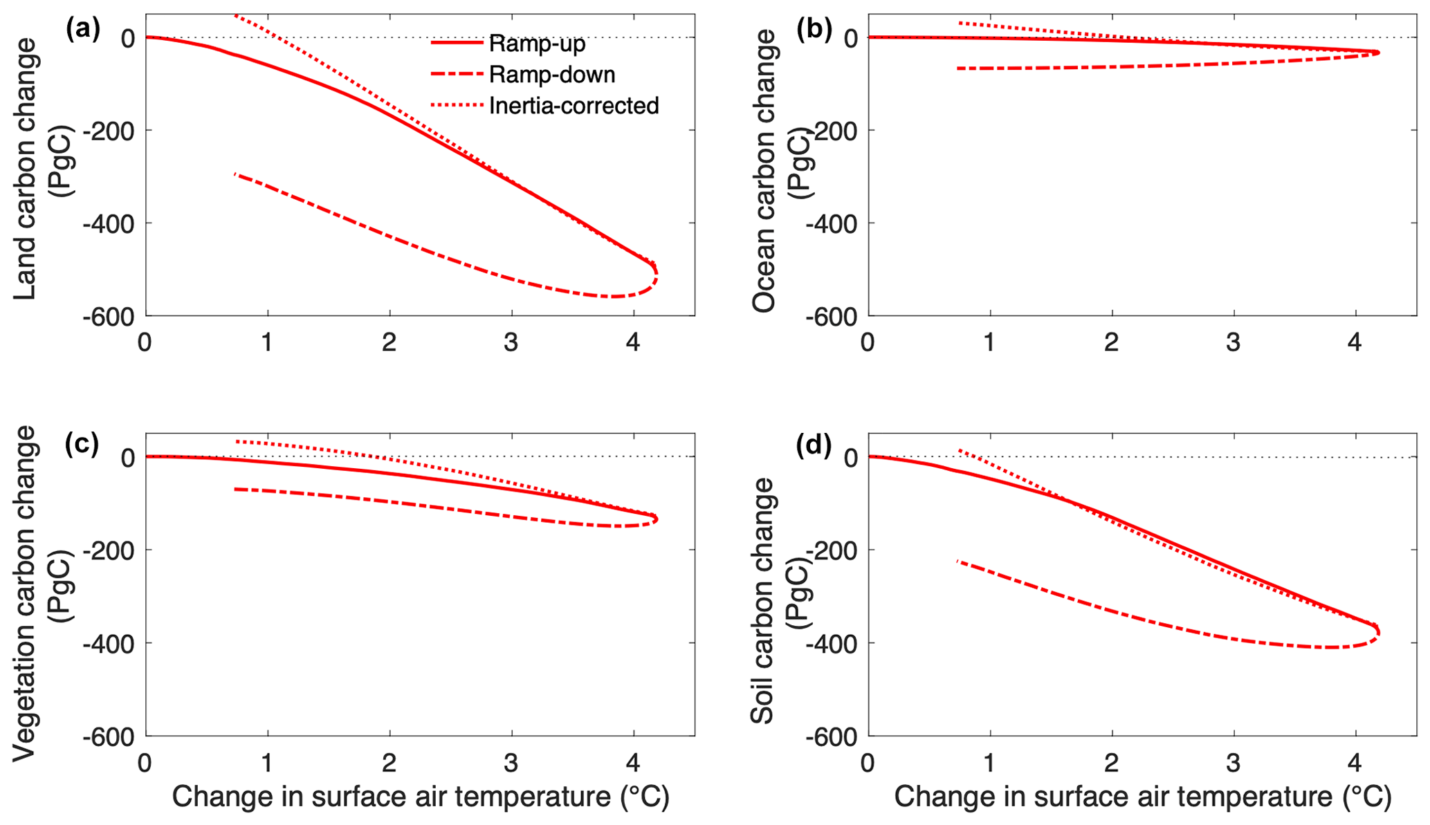
Figure 6(a) Land, (b) ocean, (c) vegetation, and (d) soil carbon pool changes as a function of surface air temperature change, taken from the radiatively coupled (RAD) CDR-reversibility simulation ramp-up and ramp-down phases and the inertia-corrected approach. All values are calculated relative to 1850 (preindustrial).
3.1.6 Carbon cycle feedback parameters quantified from CDR-reversibility simulations
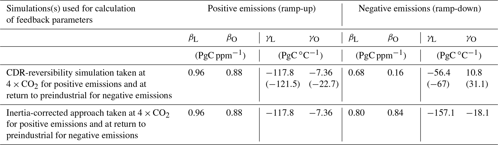
Table 1 shows the carbon cycle feedback parameters quantified using the Friedlingstein et al. (2006) carbon cycle feedback framework (see Sect. 2.4). The concentration–carbon feedback parameter (β), which quantifies the concentration–carbon feedback, is computed as the change in land or ocean carbon per unit change in atmospheric CO2 concentration in the BGC mode. The climate–carbon feedback parameter (γ) quantifies the climate–carbon feedback as the change in land or ocean carbon per unit change in surface air temperature in the RAD mode (referred to as the RAD approach). An alternative approach to quantifying the climate–carbon feedback involves taking the difference between the fully coupled and biogeochemically coupled simulations and computing the change in land or ocean carbon per unit change in surface air temperature from that difference (referred to here as the FULL–BGC approach).
In the CDR-reversibility simulation, the magnitudes of β and γ for both land and ocean are smaller in the ramp-down phase (under negative emissions) than in the ramp-up phase (under positive emissions), except the ocean climate–carbon feedback parameter, which is larger (Table 1). Climate–carbon feedback parameters calculated using the FULL–BGC approach (shown in parentheses) are consistent in sign with those calculated using the RAD approach, but the magnitudes of these feedback parameters are larger (see Fig. S5 for hysteresis figures for this approach). Carbon cycle feedback parameters are smaller in the ramp-down phase because the land and ocean carbon pools show a lagged response to changes in CO2 concentration and climate in the early ramp-down phase. In the ocean, this lagged response to changes in climate is much greater, and carbon loss continues throughout the ramp-down phase (shown by the positive ocean climate–carbon feedback parameter). As a result, feedback parameters in the ramp-down phase are underestimated. Improving this quantification could be achieved by quantifying and removing this inertia.
Table 1Carbon cycle feedback parameters under positive and negative emissions quantified at 4×CO2 (quadruple the preindustrial CO2 level) from the CDR-reversibility simulation and using the proposed inertia-corrected approach. Feedback parameters for negative emissions are positive for land or ocean carbon loss and negative for land or ocean carbon gain, opposite to the sign convention for feedbacks under positive emissions. Values shown in parentheses were calculated using the FULL–BGC approach for quantifying climate–carbon feedbacks (see Eq. 7). Feedback parameters quantified from the CDR-reversibility simulation can also be derived from Figs. 5 and 6 respectively by taking the slope of the land or ocean response at the same time points at which they are computed.
3.2 Isolating carbon cycle feedbacks under negative emissions
3.2.1 Zeroemit simulation: quantifying climate system inertia
Zero emission simulations quantify committed changes due to the prior CO2 trajectory. Changes in atmospheric CO2 concentration in zero emission simulations are driven by the carbon sinks, which in turn are influenced by the CO2 concentration and climate. Following cessation of emissions, the CO2 concentration in the FULL mode declines steadily, mainly driven by ocean carbon uptake consistent with results from MacDougall et al. (2020) (Fig. 7a). The CO2 concentration in the BGC mode declines more than in the FULL mode because both land and ocean remain carbon sinks. In the RAD mode, the CO2 concentration increases as both land and ocean carbon decrease, releasing CO2 into the atmosphere. Changes in atmospheric CO2 concentration, together with changes in ocean heat uptake and surface albedo, drive changes in surface air temperature. In the FULL mode, the warming effect of declining ocean heat uptake dominates over the cooling effect of declining CO2 concentration, resulting in continued warming (MacDougall et al., 2020) (Figs. 7b, S6). The decline in CO2 concentration is partly offset by permafrost carbon release from the soil (Fig. 7e). Surface air temperature in the RAD mode increases more than in the FULL mode because the CO2 concentration increases, causing further warming. Surface air temperature remains relatively constant in the BGC mode. In the FULL mode, the land switches into a source of carbon after emissions cease, consistent with the behaviour of the UVic ESCM in the Zero Emissions Commitment Model Intercomparison Project (ZECMIP; MacDougall et al., 2020) (Fig. 7c). Vegetation carbon continues to increase (Fig. 7d), whereas soil carbon decreases (Fig. 7e). The ocean remains a carbon sink after cessation of emissions (Fig. 7f). In the BGC mode, the ocean remains a strong carbon sink after CO2 emissions are set to zero, whereas land carbon initially increases then decreases (Fig. 7c, f). Vegetation carbon increases throughout the zero emission phase, whereas soil carbon initially increases then slowly decreases (Fig. 7d, e). Both land and ocean carbon decrease in the RAD mode (Fig. 7c, f) with both vegetation and soil carbon pools driving this decrease (Fig. 7d, e).
3.2.2 Inertia-corrected approach: isolating the response to negative emissions
The inertia-corrected approach uses the zero emission simulations described in the previous section to isolate the response to negative emissions in the CDR-reversibility simulations by taking the difference between the ramp-down phase of the RAD (BGC) CDR-reversibility simulation and the RAD (BGC) zero emission simulation. In the BGC mode, despite our attempt to reduce climate system inertia in our novel approach, carbon pools do not return to their preindustrial states at the time that atmospheric CO2 returns to preindustrial levels (Fig. 5). In the RAD mode, all carbon pools eventually gain more carbon than they held at their preindustrial states (Fig. 6).
The inertia-corrected approach removes the initial carbon increase in the CDR-reversibility BGC mode (Fig. 5) and removes the initial carbon decrease in the CDR-reversibility RAD mode (Fig. 6), reducing the width of the hysteresis. Zickfeld et al. (2016) used zero emissions to isolate the response to negative emissions and observed a reduction in the initial carbon change at the beginning of the ramp-down phase consistent with our results. In our approach, the hysteresis may persist because of the different configurations in which the CDR-reversibility and Zeroemit simulations were run: that is, the former were run with prescribed atmospheric CO2 concentration, whereas the latter were emissions-driven, which may also impact the quantification of the inertia. Another possibility may be irreversible changes in vegetation distribution in the CDR-reversibility ramp-down phase that are caused by state changes rather than inertia. When the CO2 decrease is prescribed, the Earth system is in a state of elevated CO2 concentration and surface air temperature, which may lead to a different vegetation response than to an equivalent CO2 increase applied from a preindustrial state (Zickfeld et al., 2021). Alternatively, the remaining hysteresis may show that the linearity assumption made in this experiment is not satisfied; the linearity assumption made here is that the total carbon cycle response in the ramp-down phase is a linear combination of the committed response following increasing CO2 concentration and temperature, and the response is driven by the decrease in atmospheric CO2 and temperature in the ramp-down phase (see Sect. 2.4.1: Eq. 8)
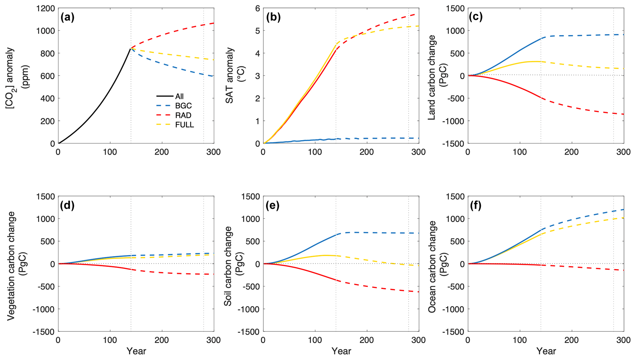
Figure 7(a) Atmospheric CO2 concentration anomaly, (b) surface air temperature anomaly, (c) land carbon change, (d) vegetation carbon change, (e) soil carbon change, and (f) ocean carbon change for the zero emission simulations relative to 1850 (preindustrial). ALL denotes the CDR-reversibility ramp-up phase from which all modes are initialized; BGC – biogeochemically coupled, RAD – radiatively coupled, and FULL – fully coupled. Solid lines are for the ramp-up phase; dashed lines are for the zero emission phase.
After isolating the response to negative emissions alone in the inertia-corrected approach, the magnitudes of βL and βO are smaller in the ramp-down phase as compared to their respective magnitudes in the ramp-up phase, but the magnitudes of γL and γO become larger in the ramp-down phase (Table 1). In the ramp-down phase, the magnitudes of β and γ from our novel approach are larger compared to those from the CDR-reversibility simulation, implying greater land and ocean carbon loss due to changes in CO2 concentration alone and greater land and ocean carbon gain due to changes in climate alone. For example, a decrease in atmospheric CO2 of 1 ppm would result in the loss of 0.68 PgC of land carbon in the standard approach and 0.80 PgC of land carbon in our approach due to changes in CO2 concentration alone, whereas cooling by 1 ∘C would result in land carbon gain of 56.4 PgC in the standard approach and almost 3 times as much (157.1 PgC) in our approach due to changes in climate alone.
Our results from the CDR-reversibility simulation show that, due to changes in CO2 concentration alone, carbon pools take up carbon in the ramp-up phase, continue to take up carbon in the early ramp-down phase, then switch into sources of carbon. Due to changes in climate alone, carbon pools lose carbon in the ramp-up phase, continue to lose carbon in the ramp-down phase, then switch into carbon sinks. Furthermore, the land and ocean carbon pools do not return to their preindustrial states at the end of both modes, suggesting that land and ocean carbon changes in the ramp-up phase are irreversible on centennial timescales. The differences in the magnitudes of carbon cycle feedbacks in the ramp-up and ramp-down phases, as quantified by feedback parameters, are likely largely due to climate system inertia. This inertia generally reduces the magnitude of both feedbacks in the ramp-down phase (under negative emissions) relative to feedbacks in the ramp-up phase (under positive emissions), implying reduced land and ocean carbon loss due to changes in CO2 concentration alone and reduced land carbon gain due to the changes in climate. The exception is the ocean that continues to lose carbon in the ramp-down phase, implying increased carbon loss due to changes in climate alone.
To quantify the carbon cycle inertia, that is, the response to the prior increasing CO2 trajectory, we ran zero emission simulations in fully coupled, biogeochemically coupled, and radiatively coupled modes. Consistent with previous studies, the ocean continues to sequester carbon in the fully coupled zero emission simulation (MacDougall et al., 2020). The terrestrial biosphere switches into a carbon source after emissions cease. Carbon uptake, largely by the ocean sink, decreases the atmospheric CO2 concentration. Surface air temperature increases due to the interplay between declining CO2 concentration and ocean heat uptake (Matthews and Caldeira, 2008; Solomon et al., 2009; Arora et al., 2013). While the carbon cycle response is consistent with the behaviour of the UVic ESCM in the Zero Emissions Commitment Model Intercomparison Project (ZECMIP; MacDougall et al., 2020), the UVic ESCM response in ZECMIP is noticeably different from the rest of the Earth system models. On centennial timescales, the UVic ESCM is the only model with a positive zero emissions commitment. However, most of the other models do not represent permafrost carbon. The carbon pools in the biogeochemically coupled and radiatively coupled zero emission simulations also exhibit inertia: the land and ocean carbon pools continue to grow after cessation of emissions in the biogeochemically coupled simulation, whereas both carbon pools reduce in the radiatively coupled simulation.
Assuming linearity in the response to increasing and decreasing CO2 concentrations (see Sect. 2.4.1: Eq. 8), we subtract the zero emission simulations from the CDR-reversibility simulations, to isolate the response to negative emissions alone. We find that in the ramp-down phase, the magnitudes of β and γ from our novel approach are generally larger as compared to those from the CDR-reversibility simulation, implying greater land and ocean carbon loss due to changes in CO2 concentration and greater land and ocean carbon gain due to changes in climate if feedback parameters from our approach are applied instead. Furthermore, land and ocean carbon changes in the ramp-up phase remain irreversible in our simulations.
A similar feedback analysis was conducted for ocean carbon cycle feedbacks using the Norwegian Earth System Model (NorESM; Schwinger and Tjiputra, 2018). Schwinger and Tjiputra calculated ocean concentration–carbon and climate–carbon feedback parameters using the same carbon cycle feedback framework and CDR-reversibility simulations used here. Their results also show a lagged ocean carbon response to the prior increasing CO2 trajectory in the ramp-down phase, and as a result, the magnitude of both carbon cycle feedbacks is smaller in the ramp-down phase than in the ramp-up phase.
We compare carbon cycle feedback parameters quantified from the CDR-reversibility ramp-up phase to model means and standard deviations from CMIP5 and CMIP6 – the fifth and sixth phases of the Coupled Model Intercomparison Project, respectively (Arora et al., 2020) (see Table S1 in the Supplement). The concentration–carbon feedback parameter for land (βL) is generally consistent with those from CMIP5 and CMIP6, while the ocean concentration–carbon feedback parameter (βO) lies slightly above the CMIP6 range (mean ± 1 standard deviation). The land climate–carbon feedback parameter (γL) lies well above the CMIP5 and CMIP6 ranges, implying a stronger sensitivity to warming relative to CMIP5 and CMIP6 models. The ocean climate–carbon feedback parameter (γO) lies slightly above the ranges for CMIP5 and CMIP6. We have included feedback parameters in the Supplement at twice the preindustrial CO2 concentration (2×CO2), which are more relevant, in terms of atmospheric CO2 levels and warming, for real-world mitigation scenarios (Table S2).
We use the UVIC ESCM, an EMIC, due to the number of simulations and length of model integration required in this study. Compared to comprehensive Earth system models, EMICs generally have coarser resolution and represent less Earth system processes at a lower level of detail. Moreover, the version of the UVic ESCM used here does not represent the nitrogen cycle on land and its coupling to the carbon cycle, which has ramifications for the estimated magnitude of carbon cycle feedbacks. Models without a nitrogen cycle exhibit greater land carbon gain under increasing CO2 concentrations relative to other CMIP5 and CMIP6 models: that is, the concentration–carbon feedback parameter is more positive (Table S1). They also exhibit greater carbon loss under increasing CO2 concentrations: that is, the climate–carbon feedback parameter is more negative. Therefore, the magnitude of both carbon cycle feedbacks in this study is generally larger under increasing CO2 concentrations relative to other CMIP5 and CMIP6 models with a nitrogen cycle. Due to the exclusion of the nitrogen cycle, the UVic ESCM is expected to exhibit greater land carbon gain due to changes in climate alone under decreasing CO2 concentrations relative to CMIP5 and CMIP6 models with a nitrogen cycle. Nitrogen mineralization will likely decline as surface air temperature declines, reducing land carbon gain due to changes in climate alone in a model with the nitrogen cycle. The direction of land carbon change due to changes in CO2 concentration alone is less certain. With the consideration of nitrogen limitation, the already weakened CO2 fertilization effect under declining CO2 concentrations could be further constrained, exacerbating the carbon loss due to changes in CO2 concentration alone. However, this may be counteracted by an enhanced rate of photosynthesis as declining CO2 concentrations decrease carbon–nitrogen ratios.
Each of the two approaches used here to quantify carbon cycle feedback parameters has its benefits and drawbacks. Because the CDR-reversibility simulation is commonly used in literature (Schwinger and Tjiputra, 2018; Keller et al., 2018; Zickfeld et al., 2016), it allows easier comparison of results across models. However, research shows that this idealized scenario may delay the land sink-to-source transition and underestimate ocean carbon uptake and the strength of the permafrost carbon feedback (MacDougall, 2019). Furthermore, this scenario requires a period of high positive emissions followed immediately by a period of high negative emissions. The yearly rate of increase in atmospheric CO2 concentration (1 % yr−1) in the ramp-up phase is twice the rate inferred from historical data (MacDougall, 2019), and achieving such a strong peak and decline is highly unlikely given the scale of negative emission technologies required.
In their 2016 paper, Zickfeld et al. used zero emission simulations to correct for the thermal and carbon cycle inertia in a suite of CDR-reversibility simulations, similar to our novel approach in this study. This reduced, but did not eliminate the climate system inertia, consistent with our results. Although our approach does not eliminate the inertia, it provides a more accurate estimate of the magnitude of carbon cycle feedbacks in the ramp-down phase by reducing the response to the prior CO2 trajectory, bringing the estimate closer to a quantification of carbon cycle feedbacks under negative emissions alone. The remaining inertia may be associated with the different configurations in which the CDR-reversibility and Zeroemit simulations were run: the former were run in concentration-driven mode, whereas the latter were emissions-driven. Therefore, changes in land and ocean carbon fluxes affect the atmospheric CO2 concentration in the zero emission simulations but not in the CDR-reversibility simulations. Alternatively, the remaining inertia may be related to irreversible changes in vegetation distribution in the CDR-reversibility simulations. Lastly, the linearity assumption made in this experimental design (Sect. 2.4.1, Eq. 8) may not hold: that is, the total carbon cycle response in the ramp-down phase may not be a linear combination of the committed response following increasing CO2 concentration and temperature as well as the response driven by the decrease in atmospheric CO2 and temperature in the ramp-down phase. If the responses to increasing and decreasing CO2 concentrations are not additive, then the zero emission simulations may not quantify and remove all the inertia in the CDR-reversibility simulations.
Carbon cycle feedbacks under negative emissions have previously been quantified from the ramp-down phase of the CDR-reversibility simulation. However, this approach underestimates the magnitudes of carbon cycle feedbacks because the response in the ramp-down phase includes climate system inertia effects that generally weaken both feedbacks. Our novel approach aims to reduce the inertia in the ramp-down phase, thereby improving the quantification of carbon cycle feedbacks under negative emissions. We find that the magnitudes of the concentration–carbon and climate–carbon feedbacks under negative emissions are larger in our approach as compared to the standard approach. The concentration–carbon feedback drives greater land and ocean carbon release under negative emissions in our approach than in the standard approach. The climate–carbon feedback promotes more land and ocean carbon sequestration in our approach than in the standard approach. This has two implications: using feedback parameters from the standard approach will (1) underestimate land and ocean carbon release under negative emissions due to changes in CO2 concentration alone (concentration–carbon feedback) and (2) underestimate land and ocean carbon gain due to changes in climate alone (climate–carbon feedback). Given that the concentration–carbon feedback is the dominant feedback, quantifying carbon cycle feedbacks under negative emissions from the CDR-reversibility simulation will result in the underestimation of carbon loss under negative emissions, thereby overestimating the effectiveness of negative emissions in drawing down CO2.
Future research should test the robustness of these results in a multi-model framework. A first step could be analysing the CDR-reversibility simulations in three modes (biogeochemically coupled, radiatively coupled, and fully coupled) in the next CMIP phase. In addition, increasing and decreasing CO2 trajectories could be applied from an equilibrium state to overcome issues related to climate system inertia.
The UVic ESCM (University of Victoria Earth System Climate Model) data are stored at https://doi.org/10.20383/102.0732 (Chimuka et al., 2023), and the model code for UVic ESCM 2.10 is available at http://terra.seos.uvic.ca/model/2.10/ (Earth System Climate Model, 2023).
The supplement related to this article is available online at: https://doi.org/10.5194/bg-20-2283-2023-supplement.
KZ developed the research question and worked with CMN on the initial data analysis. VRC ran the model simulations and worked with KZ to analyse and interpret the model data and write the paper. CMN also helped to revise the paper.
The contact author has declared that none of the authors has any competing interests.
Publisher’s note: Copernicus Publications remains neutral with regard to jurisdictional claims in published maps and institutional affiliations.
Computing resources were provided by the Digital Research Alliance of Canada (formerly Compute Canada).
This research has been supported by the Natural Sciences and Engineering Research Council of Canada (grant no. RGPIN-2018-06881).
This paper was edited by Sara Vicca and reviewed by two anonymous referees.
Arora, V. K., Boer, G. J., Friedlingstein, P., Eby, M., Jones, C. D., Christian, J. R., Bonan, G., Bopp, L., Brovkin, V., Cadule, P., Hajima, T., Ilyina, T., Lindsay, K., Tjiputra, J. F., and Wu, T.: Carbon–Concentration and Carbon–Climate Feedbacks in CMIP5 Earth System Models, J. Climate, 26, 5289–5314, https://doi.org/10.1175/JCLI-D-12-00494.1, 2013.
Arora, V. K., Katavouta, A., Williams, R. G., Jones, C. D., Brovkin, V., Friedlingstein, P., Schwinger, J., Bopp, L., Boucher, O., Cadule, P., Chamberlain, M. A., Christian, J. R., Delire, C., Fisher, R. A., Hajima, T., Ilyina, T., Joetzjer, E., Kawamiya, M., Koven, C. D., Krasting, J. P., Law, R. M., Lawrence, D. M., Lenton, A., Lindsay, K., Pongratz, J., Raddatz, T., Séférian, R., Tachiiri, K., Tjiputra, J. F., Wiltshire, A., Wu, T., and Ziehn, T.: Carbon–concentration and carbon–climate feedbacks in CMIP6 models and their comparison to CMIP5 models, Biogeosciences, 17, 4173–4222, https://doi.org/10.5194/bg-17-4173-2020, 2020.
Boer, G. J. and Arora, V.: Geographic Aspects of Temperature and Concentration Feedbacks in the Carbon Budget, J. Climate, 23, 775–784, https://doi.org/10.1175/2009JCLI3161.1, 2010.
Boer, G. J. and Arora, V.: Feedbacks in emission-driven and concentration-driven global carbon budgets, J. Climate, 32, 3326–3341, https://doi.org/10.1175/JCLI-D-12- 00365.1, 2013.
Boucher, O., Halloran, P. R., Burke, E. J., Doutriaux-Boucher, M., Jones, C. D., Lowe, J. Ringer, M. A., Robertson, E., and Wu, P.: Reversibility in an earth system model in response to CO2 concentration changes, Environ. Res. Lett., 7, 024013, https://doi.org/10.1088/1748-9326/7/2/024013, 2012.
Cao, L. and Caldeira, K.: Atmospheric carbon dioxide removal: Long term consequences and commitment, Environ. Res. Lett., 5, 024011, https://doi.org/10.1088/1748-9326/5/2/024011, 2010.
Canadell, J. G., Monteiro, P. M. S., Costa, M. H., Cotrim da Cunha, L., Cox, P. M., Eliseev, A. V., Henson, S., Ishii, M., Jaccard, S., Koven, C., Lohila, A., Patra, P.K., Piao, S., Rogelj, J., Syampungani, S., Zaehle, S., and Zickfeld, K.: Global Carbon and other Biogeochemical Cycles and Feedbacks, in: Climate Change 2021: The Physical Science Basis, Contribution of Working Group I to the Sixth Assessment Report of the Intergovernmental Panel on Climate Change, ediyed by: Masson-Delmotte, V., Zhai, P., Pirani, A., Connors, L. C., Berger, S., Caud, N., Chen, Y., Goldfarb, L., Gomis, M. I., Huang, M., Leitzell, K., Lonnoy, E., Matthews, J. B. R., Maycock, T. K., Waterfield, T., Yeleki, O., Yu, R., and Zhou, B., Cambridge University Press, Cambridge, United Kingdom and New York, NY, USA, 673–816, https://doi.org/10.1017/9781009157896.007, 2021
Chimuka, V., Nzotungicimpaye, C., and Zickfeld, K.: Quantifying land carbon cycle feedbacks under negative CO2 emissions – Supplementary Data, Federated Research Data Repository [data set], last access: 31 May 2023, https://doi.org/10.20383/102.0732, 2023.
Ciais, P., Sabine, C., Bala, G., Bopp, L., Brovkin, V., Canadell, J., Chhabra, A., DeFries, R., Galloway, J., Heimann, M., Jones, C., Le Queìreì, C., Myneni, R. B., Piao, S., and Thornton, P.: Carbon and Other Biogeochemical Cycles, in: Working Group I Contribution to the Intergovernmental Panel on Climate Change Fifth Assessment Report Climate Change 2013: The Physical Science Basis, edited by: Stocker, T. F., Qin, D., Plattner, G.-K., Tignor, M., Allen, S. K., Boschung, J., Nauels, A., Xia, Y., Bex, V., and Midgley, P., Cambridge University Press, https://www.ipcc.ch/site/assets/uploads/2018/02/WG1AR5_Chapter06_FINAL.pdf (last access: February 2022), 2013.
Cox, P. M., Betts, R. A., Jones. C.D., Spall, S. A., and Totterdell, I.: Acceleration of global warming due to carbon-cycle feedbacks in a coupled climate model, Nature, 408, 184–187, https://doi.org/10.1038/35041539, 2000.
Cox, P.: Description of the TRIFFID Dynamic Global Vegetation Model, Hadley Centre Technical Note # 24, UK Met Office, https://digital.nmla.metoffice.gov.uk/IO_cc8f146a-d524-4243-88fc-e3a3bcd782e7/ (last access: June 2022), 2001.
Earth System Climate Model: UVic ESCM [code], https://terra.seos.uvic.ca/model/2.10/, last access: 31 May 2023.
Eby, M., Weaver, A. J., Alexander, K., Zickfeld, K., Abe-Ouchi, A., Cimatoribus, A. A., Crespin, E., Drijfhout, S. S., Edwards, N. R., Eliseev, A. V., Feulner, G., Fichefet, T., Forest, C. E., Goosse, H., Holden, P. B., Joos, F., Kawamiya, M., Kicklighter, D., Kienert, H., Matsumoto, K., Mokhov, I. I., Monier, E., Olsen, S. M., Pedersen, J. O. P., Perrette, M., Philippon-Berthier, G., Ridgwell, A., Schlosser, A., Schneider von Deimling, T., Shaffer, G., Smith, R. S., Spahni, R., Sokolov, A. P., Steinacher, M., Tachiiri, K., Tokos, K., Yoshimori, M., Zeng, N., and Zhao, F.: Historical and idealized climate model experiments: an intercomparison of Earth system models of intermediate complexity, Clim. Past, 9, 1111–1140, https://doi.org/10.5194/cp-9-1111-2013, 2013.
Eyring, V., Bony, S., Meehl, G. A., Senior, C. A., Stevens, B., Stouffer, R. J., and Taylor, K. E.: Overview of the Coupled Model Intercomparison Project Phase 6 (CMIP6) experimental design and organization, Geosci. Model Dev., 9, 1937–1958, https://doi.org/10.5194/gmd-9-1937-2016, 2016.
Friedlingstein, P., Cox, P., Betts, R., Bopp, L., Von Bloh, W., Brovkin, V., Cadule, P., Doney, S., Eby, M., Fung, I., Bala, G., John, J., Jones, C., Joos, F., Kato, T., Kawamiya, M., Knorr, W., Lindsay, K., Matthews, H. D., Raddatz, T., Rayner, P., Reick, C., Roeckner, E., Schnitzler, K.-G., Schnur, R., Strassmann, K., Weaver, A. J., Yoshikawa, C., Zeng, A. N., and Friedlingstein, P.: Climate–Carbon Cycle Feedback Analysis: Results from the C4 MIP Model Intercomparison, J. Climate, 19, 3337–3353, doi.org/10.1175/JCLI3800.1, 2006.
Friedlingstein, P., O'Sullivan, M., Jones, M. W., Andrew, R. M., Gregor, L., Hauck, J., Le Quéré, C., Luijkx, I. T., Olsen, A., Peters, G. P., Peters, W., Pongratz, J., Schwingshackl, C., Sitch, S., Canadell, J. G., Ciais, P., Jackson, R. B., Alin, S. R., Alkama, R., Arneth, A., Arora, V. K., Bates, N. R., Becker, M., Bellouin, N., Bittig, H. C., Bopp, L., Chevallier, F., Chini, L. P., Cronin, M., Evans, W., Falk, S., Feely, R. A., Gasser, T., Gehlen, M., Gkritzalis, T., Gloege, L., Grassi, G., Gruber, N., Gürses, Ö., Harris, I., Hefner, M., Houghton, R. A., Hurtt, G. C., Iida, Y., Ilyina, T., Jain, A. K., Jersild, A., Kadono, K., Kato, E., Kennedy, D., Klein Goldewijk, K., Knauer, J., Korsbakken, J. I., Landschützer, P., Lefèvre, N., Lindsay, K., Liu, J., Liu, Z., Marland, G., Mayot, N., McGrath, M. J., Metzl, N., Monacci, N. M., Munro, D. R., Nakaoka, S.-I., Niwa, Y., O'Brien, K., Ono, T., Palmer, P. I., Pan, N., Pierrot, D., Pocock, K., Poulter, B., Resplandy, L., Robertson, E., Rödenbeck, C., Rodriguez, C., Rosan, T. M., Schwinger, J., Séférian, R., Shutler, J. D., Skjelvan, I., Steinhoff, T., Sun, Q., Sutton, A. J., Sweeney, C., Takao, S., Tanhua, T., Tans, P. P., Tian, X., Tian, H., Tilbrook, B., Tsujino, H., Tubiello, F., van der Werf, G. R., Walker, A. P., Wanninkhof, R., Whitehead, C., Willstrand Wranne, A., Wright, R., Yuan, W., Yue, C., Yue, X., Zaehle, S., Zeng, J., and Zheng, B.: Global Carbon Budget 2022, Earth Syst. Sci. Data, 14, 4811–4900, https://doi.org/10.5194/essd-14-4811-2022, 2022.
Friedlingstein, P., Meinshausen, M., Arora, V., Jones, C., Anav, A., Liddicoat, S., and Knutti, R.: Uncertainties in CMIP5 climate projections due to carbon cycle feedbacks, J. Climate, 27, 511–526, https://doi.org/10.1175/JCLI-D-12-00579.1, 2014.
Fung, I.Y., Doney, S. C., Lindsay, K., and Jasmin J. G.: Evolution of carbon sinks in a changing climate, P. Natl. Acad. Sci. USA, 102, 11201–11206, https://doi.org/10.1073/pnas.0504949102, 2005.
Fuss, S., Canadell, J. G., Peters, G. P., Tavoni, M., Andrew, R. M. Ciais, P., Jackson, R. B., Jones, C. D., Kraxner, F., Nakicenovic, N., Le Quéré, C., Raupach, M. R., Sharifi, A., Smith P., and Yamagata, Y.: Betting on negative emissions, Nat. Clim. Change, 4, 850–853, doi.org/10.1038/nclimate2392, 2014.
IPCC: Climate Change 2022: Impacts, Adaptation, and Vulnerability, Contribution of Working Group II to the Sixth Assessment Report of the Intergovernmental Panel on Climate Change, edited by: Pörtner, H.-O. Roberts, D. C., Tignor, M., Poloczanska, E. S., Mintenbeck, K., Alegría, A., Craig, M., Langsdorf, S., Löschke, S., Möller, V., Okem, A., Rama, B., Cambridge University Press, in Press, https://doi.org/10.1017/9781009325844, 2022.
Jeltsch-Thömmes, A., Stocker, T. F., and Joos, F.: Hysteresis of the Earth system under positive and negative CO2 emissions, Environ. Res. Lett., 15, 124026, https://doi.org/10.1088/1748-9326/abc4af, 2020.
Jones, C. D., Arora, V., Friedlingstein, P., Bopp, L., Brovkin, V., Dunne, J., Graven, H., Hoffman, F., Ilyina, T., John, J. G., Jung, M., Kawamiya, M., Koven, C., Pongratz, J., Raddatz, T., Randerson, J. T., and Zaehle, S.: C4MIP – The Coupled Climate–Carbon Cycle Model Intercomparison Project: experimental protocol for CMIP6, Geosci. Model Dev., 9, 2853–2880, https://doi.org/10.5194/gmd-9-2853-2016, 2016.
Jones, C. D., Ciais, J., Davis, S. J., Friedlingstein, P., Gasser, T., Peters, G. P., and Wiltshire, A.: Simulating the Earth System response to negative emissions, Environ. Res. Lett., 11, 095012, https://doi.org/10.1088/1748-9326/11/9/095012, 2016.
Jones, C. D., Cox, P. M., Essery, R. L. H., Roberts, D. L., and Woodage, M. J.: Strong carbon cycle feedbacks in a climate model with interactive CO2 and sulphate aerosols, Geophys. Res. Lett., 30, 1479, https://doi.org/10.1029/2003GL016867, 2003.
Keller, D. P., Lenton, A., Scott, V., Vaughan, N. E., Bauer, N., Ji, D., Jones, C. D., Kravitz, B., Muri, H., and Zickfeld, K.: The Carbon Dioxide Removal Model Intercomparison Project (CDRMIP): rationale and experimental protocol for CMIP6, Geosci. Model Dev., 11, 1133–1160, https://doi.org/10.5194/gmd-11-1133-2018, 2018.
Keller, D. P., Oschlies, A., and Eby, M.: A new marine ecosystem model for the University of Victoria Earth System Climate Model, Geosci. Model Dev., 5, 1195–1220, https://doi.org/10.5194/gmd-5-1195-2012, 2012.
Koven, C. D., Arora, V. K., Cadule, P., Fisher, R. A., Jones, C. D., Lawrence, D. M., Lewis, J., Lindsay, K., Mathesius, S., Meinshausen, M., Mills, M., Nicholls, Z., Sanderson, B. M., Séférian, R., Swart, N. C., Wieder, W. R., and Zickfeld, K.: Multi-century dynamics of the climate and carbon cycle under both high and net negative emissions scenarios, Earth Syst. Dynam., 13, 885–909, https://doi.org/10.5194/esd-13-885-2022, 2022.
MacDougall, A. H.: Limitations of the 1 % experiment as the benchmark idealized experiment for carbon cycle intercomparison in C4MIP, Geosci. Model Dev., 12, 597–611, https://doi.org/10.5194/gmd-12-597-2019, 2019.
MacDougall, A. H. and Knutti, R.: Projecting the release of carbon from permafrost soils using a perturbed parameter ensemble modelling approach, Biogeosciences, 13, 2123–2136, https://doi.org/10.5194/bg-13-2123-2016, 2016.
MacDougall, A. H., Frölicher, T. L., Jones, C. D., Rogelj, J., Matthews, H. D., Zickfeld, K., Arora, V. K., Barrett, N. J., Brovkin, V., Burger, F. A., Eby, M., Eliseev, A. V., Hajima, T., Holden, P. B., Jeltsch-Thömmes, A., Koven, C., Mengis, N., Menviel, L., Michou, M., Mokhov, I. I., Oka, A., Schwinger, J., Séférian, R., Shaffer, G., Sokolov, A., Tachiiri, K., Tjiputra, J., Wiltshire, A., and Ziehn, T.: Is there warming in the pipeline? A multi-model analysis of the Zero Emissions Commitment from CO2, Biogeosciences, 17, 2987–3016, https://doi.org/10.5194/bg-17-2987-2020, 2020.
Matthews, H. D. and Caldeira, K.: Stabilizing climate requires near–zero emissions, Geophys. Res. Lett., 35, L04705, https://doi.org/10.1029/2007GL032388, 2008.
Meissner, K. J., Weaver, A. J., Matthews, H. D., and Cox, P. M.: The role of land surface dynamics in glacial inception: a study with the UVic Earth System Model, Clim. Dynam., 21, 515–537, https://doi.org/10.1007/s00382-003-0352-2, 2003.
Melnikova, I., Boucher, O., Cadule, P., Ciais, P., Gasser, T., Quilcaille, Y., Shiogama, H., Tachiiri, K., Yokohata, T. and Tanaka, K.: Carbon cycle response to temperature overshoot beyond 2 ∘C: An analysis of CMIP6 models, Earth's Future, 9, e2020EF001967, https://doi.org/10.1029/2020EF001967, 2021.
Mengis, N., Keller, D. P., MacDougall, A. H., Eby, M., Wright, N., Meissner, K. J., Oschlies, A., Schmittner, A., MacIsaac, A. J., Matthews, H. D., and Zickfeld, K.: Evaluation of the University of Victoria Earth System Climate Model version 2.10 (UVic ESCM 2.10), Geosci. Model Dev., 13, 4183–4204, https://doi.org/10.5194/gmd-13-4183-2020, 2020.
Pacanowski, R. C.: MOM 2 Documentation, users guide and reference manual, GFDL Ocean Group Technical Report 3, Geophys, Fluid Dyn. Lab., Princet. Univ. Princeton, NJ, https://www.gfdl.noaa.gov/wp-content/uploads/2016/10/manual2.2.pdf (last access: February 2022), 1995.
Park, S. and Kug, J.: A decline in atmospheric CO2 levels under negative emissions may enhance carbon retention in the terrestrial biosphere, Commun. Earth. Environ., 3, 289, https://doi.org/10.1038/s43247-022-00621-4, 2022
Rogelj, J., Shindell, D., Jiang, K., Fifita, S., Forster, P., Ginzburg, V., Handa, C., Kheshgi, H., Kobayashi, S., Kriegler, E., Mundaca, L., Seferian, R., and Vilarino, M. V.: Mitigation Pathways Compatible with 1.5 ?C in the Context of Sustainable Development, in: Global Warming of 1.5 ?C. An IPCC Special Report on the impacts of global warming of 1.5 ?C above pre-industrial levels and related global greenhouse gas emission pathways, in the context of strengthening the global response to the threat of climate change, sustainable development, and efforts to eradicate poverty, edited by: Masson-Delmotte, V., Zhai, P., Pörtner, H.-O., Roberts, D., Skea, J., Shukla, P. R., Pirani, A., Moufouma-Okia, W., Péan, C., Pidcock, R., Connors, S., Matthews, J. B. R., Chen, Y., Zhou, X., Gomis, M. I., Lonnoy, E., Maycock, T., Tignor, M., and Waterfield, T., Cambridge University Press, Cambridge, UK and New York, NY, USA, 93–174, https://doi.org/10.1017/9781009157940.004, 2018.
Rogelj, J., Forster, P. M., Kriegler, E., Smith, C. J., and Séférian, R.: Estimating and tracking the remaining carbon budget for stringent climate targets, Nature, 571, 335–342, https://doi.org/10.1038/s41586-019-1368-z, 2019
Schwinger, J. and Tjiputra, J.: Ocean Carbon Cycle Feedbacks Under Negative Emissions, Geophys. Res. Lett., 45, 5062–5070, https://doi.org/10.1029/2018GL077790, 2018.
Solomon, S., Plattner, G.-K., Knutti, R., and Friedlingstein, P.: Irreversible climate change due to carbon dioxide emissions, P. Natl. Acad. Sci. USA, 106, 1704–1709, https://doi.org/10.1073/pnas.0812721106, 2009.
Tokarska, K. B. and Zickfeld, K.: The effectiveness of net negative carbon dioxide emissions in reversing anthropogenic climate change, Environ. Res. Lett., 094013, https://doi.org/10.1088/1748-9326/10/9/094013, 2015.
UNFCCC: Adoption of the Paris Agreement, https://unfccc.int/sites/default/files/resource/docs/2015/cop21/eng/l09r01.pdf (last access: 19 November 2022), 2022.
Weaver, A. J., Eby, M., Wiebe, E. C., Bitz, C. M., Duffy, P. B., Ewen, T. L., and Fanning, A. F.: The UVic Earth System Climate Model: Model description, climatology, and applications to past, present and future climates, Atmos. Ocean, 39, 361–428, 2001.
Zickfeld, K., Azevedo, D., Mathesius, S., and Matthews, H. D.: Asymmetry in the climate–carbon cycle response to positive and negative CO2 emissions, Nat. Clim. Change, 11, 613–617, https://doi.org/10.1038/s41558-021-01061-2, 2021.
Zickfeld, K., Eby, M., Matthews, H. D., Schmittner, A., and Weaver, A. J.: Nonlinearity of Carbon Cycle Feedbacks, J. Climate, 24, 4255–4275, https://doi.org/10.1175/2011JCLI3898.1, 2011.
Zickfeld, K., MacDougall, A. H., and Matthews, H. D.: On the proportionality between global temperature change and cumulative CO2 emissions during periods of net negative CO2 emissions, Environ. Res. Lett., 11, 055006, https://doi.org/10.1088/1748-9326/11/5/055006, 2016.
Ziehn, T., Lenton, A., and Law, R.: An assessment of land-based climate and carbon reversibility in the Australian Community Climate and Earth System Simulator, Mitig. Adapt. Strateg. Glob. Change, 25, 713–731, https://doi.org/10.1007/s11027-019-09905-1, 2020.