Mammalian bioturbation amplifies rates of both hillslope sediment erosion and accumulation along the Chilean climate gradient

Animal burrowing activity affects soil texture, bulk density, soil water content, and redistribution of nutrients. All of these parameters in turn influence sediment redistribution, which shapes the earth's surface. Hence it is important to include bioturbation into hillslope sediment transport models. However, the inclusion of burrowing animals into hillslope-wide models has thus far been limited and has largely omitted vertebrate bioturbators, which can be major agents of bioturbation, especially in drier areas.

Here, we included vertebrate bioturbator burrows into a semi-empirical Morgan–Morgan–Finney soil erosion model to allow a general approach to the assessment of the impacts of bioturbation on sediment redistribution within four sites along the Chilean climate gradient. For this, we predicted the distribution of burrows by applying machine learning techniques in combination with remotely sensed data in the hillslope catchment. Then, we adjusted the spatial model parameters at predicted burrow locations based on field and laboratory measurements. We validated the model using field sediment fences. We estimated the impact of bioturbator burrows on surface processes. Lastly, we analyzed how the impact of bioturbation on sediment redistribution depends on the burrow structure, climate, topography, and adjacent vegetation.

Including bioturbation greatly increased model performance and demonstrates the overall importance of vertebrate bioturbators in enhancing both sediment erosion and accumulation along hillslopes, though this impact is clearly staggered according to climatic conditions. Burrowing vertebrates increased sediment accumulation by 137.8 % ± 16.4 % in the arid zone (3.53 kg ha⁻¹ yr⁻¹ vs. 48.79 kg ha⁻¹ yr⁻¹), sediment erosion by 6.5 % ± 0.7 % in the semi-arid zone (129.16 kg ha⁻¹ yr⁻¹ vs. 122.05 kg ha⁻¹ yr⁻¹), and sediment erosion by 15.6 % ± 0.3 % in the Mediterranean zone (4602.69 kg ha⁻¹ yr⁻¹ vs. 3980.96 kg ha⁻¹ yr⁻¹). Bioturbating animals seem to play only a negligible role in the humid zone. Within all climate zones, bioturbation did not uniformly increase erosion or accumulation within the whole hillslope catchment. This depended on adjusting environmental parameters. Bioturbation increased erosion with increasing slope, sink connectivity, and topography ruggedness and decreasing vegetation cover and soil wetness. Bioturbation increased sediment accumulation with increasing surface roughness, soil wetness, and vegetation cover.

1 Introduction

Bioturbation was shown to shape the land surface (Hazelhoff et al., 1981; Istanbulluoglu, 2005; Taylor et al., 2019; Tucker and Hancock, 2010; Whitesides and Butler, 2016; Wilkinson et al., 2009; Corenblit et al., 2021) by influencing surface microtopography (Reichman and Seabloom, 2002; Kinlaw and Grasmueck, 2012; Debruyn and Conacher, 1994) and soil properties such as soil porosity, permeability, and infiltration (Reichman and Seabloom, 2002; Yair, 1995; Hancock and Lowry, 2021; Ridd, 1996; Hall et al., 1999; Coombes, 2016; Larsen et al., 2021). Cumulatively, these modifications lead to changes in sediment redistribution (Gabet et al., 2003; Nkem et al., 2000; Wilkinson et al., 2009) and hence have the potential to affect surface topography and nutrient redistribution on large spatial and temporal scales. To quantify these effects, the shared role of climate, landscape characteristics, and burrowing dynamics on sediment redistribution needs to be understood.

On a local scale, currently used field methods to monitor sediment redistribution under real-life conditions are mainly erosion pins, splash boards, and rainfall simulators (Imeson and Kwaad, 1976; Wei et al., 2007; Le Hir et al., 2007; G. Li et al., 2019; T. C. Li et al., 2019; T. Li et al., 2018; Voiculescu et al., 2019; Chen et al., 2021; Übernickel et al., 2021a). The monitoring of box experiments yields a high spatiotemporal resolution and can also be linked to mathematical equations, such as random walks (Boudreau, 1986; Wheatcroft et al., 1990), stochastic differential equations (Boudreau, 1989; Milstead et al., 2007), finite-difference mass balancing (Soetaert et al., 1996; François et al., 1997), and Markov chain theory (Jumars et al., 1981; Foster, 1985; Trauth, 1998; Shull, 2001) to describe sediment redistribution.

Previously used methods have, however, several limitations when studying bioturbation. Field measurements likely lead to an underestimation of sediment fluxes, as they are one-time or seasonal measurements and thus do not capture the continuous excavation of the sediment by the animal (Grigusova et al., 2022) at a high temporal resolution. Box experiments and the mathematical equations derived from them describe bioturbation as an isolated process and ignore adjacent environmental parameters (such as climate or vegetation). However, the field measurements showed both positive (Hazelhoff et al., 1981; Black and Montgomery, 1991; Chen et al., 2021) and negative impact of bioturbation on erosion (Imeson and Kwaad, 1976; Hakonson, 1999). Also, previous field-based studies observed an increased bioturbation activity with higher (Milstead et al., 2007; Meserve, 1981; Tews et al., 2004; Wu et al., 2021; Ferro and Barquez, 2009) and lower vegetation cover (Simonetti, 1989; S. Zhang et al., 2020; Q. Zhang et al., 2019; Qin et al., 2021). Furthermore, soil mixing rates are not homogenous throughout the year; they depend on the animal phenological cycles (Eccard and Herde, 2013; Jimenez et al., 1992; Katzman et al., 2018; Malizia, 1998; Morgan and Duzant, 2008; Monteverde and Piudo, 2011; Gray et al., 2020; Yu et al., 2017).

Another approach offers raster-based soil erosion and landscape evolution models which integrate co-dependencies between bioturbation-relevant environmental parameters (Black and Montgomery, 1991; Meysman et al., 2003; Yoo et al., 2005; Schiffers et al., 2011). The most common soil erosion models are empirical (Wischmeier and Smith, 1978; Williams, 1975; Renard et al., 1991), process-based (Morgan et al., 1998; Roo et al., 1996; Nearing et al., 1989; Beasley et al., 1980), and semi-empirical models, the latter of which are a combination of both (Morgan et al., 1984; Beven and Kirkby, 1979).

Process-based models are based on a mechanistic understanding of the underlying physical, chemical, and biological processes that govern the behavior of the system being studied. They must be parameterized for each site; however, these models explicitly represent the governing equations and simulate the system's behavior by numerically solving these equations. Process-based models are generally considered to be more realistic and accurate than empirical models because they capture the fundamental processes that drive the system's behavior. However, process-based models can be computationally expensive, require more data and knowledge of system properties, and may require complex numerical algorithms (Morgan et al., 1998; Roo et al., 1996; Nearing et al., 1989; Beasley et al., 1980).

Within empirical models, on the other hand, the physical equations are completely replaced by empirically determined equations which only hold for the specific area they are derived for. These models are generally simpler, are less computationally expensive, and require more data and knowledge of system properties than process-based models. However, empirical models also tend to be less accurate than process-based models, particularly when applying beyond the range of data used to fit the model. In contrast to physical-based models, empirical models may not be applicable to new or different conditions, as they are based on observed relationships and do not capture the underlying processes that govern system behavior (Wischmeier and Smith, 1978; Williams, 1975; Renard et al., 1991).

Semi-empirical models combine the advantages of the both model types (Morgan et al., 1984; Morgan, 2001; Morgan and Duzant, 2008; Devia et al., 2015; Lilhare et al., 2015). Most landscape models have not yet implemented the impacts of bioturbators on water and sediment fluxes (Brosens et al., 2020; Anderson et al., 2019; Braun et al., 2016; Cohen et al., 2010, 2015; Carretier et al., 2014; Welivitiya et al., 2019). There are numerous models describing benthic soil mixing (Francois et al., 1997, 2002; Kadko and Heath 1984; Croix et al., 2002), biodiffusion caused by all invertebrate bioturbators (Meysman et al., 2005; Rakotomalala et al., 2015; Morris et al., 2006), and vertical soil mixing and lateral sediment redistribution caused by single invertebrate species (Orvain et al., 2006; Román-Sánchez et al., 2019; Orvain, 2003, 2005; Sanford, 2008). However, there are also models which described the impact of bioturbation on sediment redistribution by vertebrate animal species, such as the impact of pocket gophers on non-linear hillslope diffusion (Gabet, 2000) or on the creation of Mima mounds (Gabet et al., 2014). Several models include soil vertical mixing caused by bioturbation and its effect on landscape evolution on a millennial scale. This rather large spatiotemporal scale, however, means an omission of the natural variability in burrow sizes and densities, climate zones, and seasonality. In these models, soil erosion increases proportionally with increasing bioturbation, vertical soil mixing rates are uniform, and bioturbation is positively linked with vegetation cover (Temme and Vanwalleghem, 2016; Vanwalleghem et al., 2013; Yoo and Mudd, 2008; Pelletier et al., 2013). None of the previous studies included vertebrate bioturbator burrows of various sizes and spatial distribution by adjusting the soil properties and topography into a raster-based area-wide soil erosion model. This approach would enable us to understand the impact of all vertebrate bioturbators by considering the spatial distribution and variable impacts of bioturbator burrows on sediment redistribution. For this, bioturbation has to be included into erosion models at a spatial resolution which allows the imitation of the surface processes occurring within and near the burrow and at a temporal resolution which captures the animal daily burrowing behavior.

A suitable model which can be extended to include continuous bioturbating activity is the semi-empirical Morgan–Morgan–Finney soil erosion model (Morgan et al., 1984; Morgan, 2001). This model was successfully tested in several climate zones and land use types, such as Mediterranean sites (Jong et al., 1999); rainfed agrosystems, fields, and pastures (López-Vicente et al., 2008); the East African Highlands (Vigiak et al., 2005); and humid forests (Vieira et al., 2014). One of the recently developed improvements of this model is the daily Morgan–Morgan–Finney model (DMMF), which introduces subsurface flow and vegetation structures (type, size, height, root depth) and enables modeling at a high spatial (0.5 m) and temporal (daily) resolution (Choi et al., 2017). These improvements yield the potential to integrate the bioturbation into the model, as the burrowing activity is not constant and depends on vegetation structure (Tews et al., 2004; Ferro and Barquez, 2009).

In this study, we include vertebrate bioturbator burrows into a semi-empirical soil erosion model (DMMF) at a daily temporal and 0.5 m spatial resolution. For this, we predict the distribution of burrows by applying machine learning techniques in combination with using remotely sensed data as predictors. Then, we adjust soil properties, topography, and vegetation properties at predicted burrow locations based on field and laboratory measurements. We validate the model using field sediment fences. We run the model for a time period of 6 years, once with and without burrow adjustments. We estimate the impact of bioturbator burrows on sediment redistribution (including accumulation, erosion, and excavation) and surface runoff within four sites along the Chilean climate gradient. Lastly, we analyze how the impact of bioturbation on sediment redistribution depends on the burrow structure, climate, topography, and adjacent vegetation. Our study shows the importance of including bioturbation into erosion modeling and describes the interplay between bioturbation, environmental parameters such vegetation and topography, and sediment redistribution.

2 Study area

Our study was performed along a climate and ecological gradient in Chile (Übernickel et al., 2021b), comprising four study sites in the Chilean Coastal Cordillera: Pan de Azúcar (PdA) National Park (NP), Santa Gracia (SG), La Campana (LC) NP, and Nahuelbuta (NA) NP (Fig. 1). PdA NP is located in the arid zone in a fog-laden environment in the southern part of the Atacama Desert, with almost no rainfall. The vegetation cover is less than 5 % and dominated by small desert shrubs, several types of cacti, and biocrusts (Lehnert et al., 2018). SG is a natural reserve located in the semi-arid zone near La Serena, which is dominated by goat grazing. The vegetation consists of shrubs and cacti, covering up to 40 % of the study area. LC NP is part of the Mediterranean-type climate zone in the Valparaíso Region and is also affected by cattle. The study site is dominated by an evergreen sclerophyllous forest with endemic palms. The canopy reaches a height of up to 9 m, and the understory consists of deciduous shrubs and herbs. NA is located in the humid–temperate zone and characterized by a dense evergreen Araucaria forest comprising broadleaved trees with heights of up to 14 m. The ground is covered by bamboo, shrubs, and herbs (Bernhard et al., 2018; Oeser et al., 2018). The most common bioturbating vertebrate animal species recorded within these sites are carnivores of the family Canidae (Lycalopex culpaeus, Lycalopex griseus) as well as rodents of the families Abrocomidae (Abrocoma bennetti), Chinchillidae (Lagidium viscacia), Cricetidae (Abrothrix andinus, Phyllotis xanthopygus, Phyllotis limatus, Phyllotis darwini), and Octodontidae (Cerqueira, 1985; Jimenez et al., 1992; Übernickel et al., 2021a).

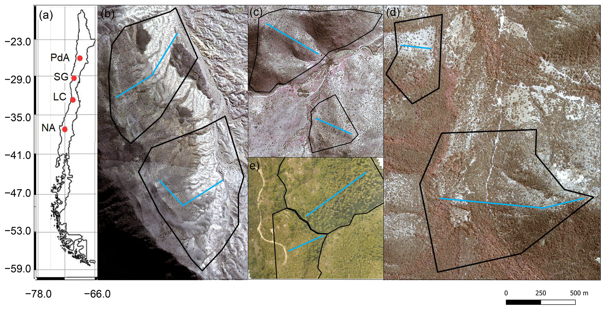
Figure 1 Study area and study sites. Black lines outline the hillslope catchments. Along the blue lines, the in situ data (mound locations, soil samples, vegetation mapping) were collected. (a) Position of the study sites along the climate gradient. PdA – Pan de Azúcar, SG – Santa Gracia, LC – La Campana, NA – Nahuelbuta. Positions of plots in (b) PdA, (c) SG, (d) LC, and (e) NA. The background image is an RGB composite calculated from WorldView-2 satellite imagery. Images were obtained with a single license from GAF AG. Scale bar is the same for (b), (c), (d), and (e).

3 Methodology

We combined semi-empirical soil erosion modeling with in situ measurements, remote sensing data, and machine learning methods (Fig. 2). Along eight hillslope catchments within four climate zones, we mapped locations of burrows, estimated the vegetation cover, and extracted soil samples. We analyzed the soil samples in the laboratory. Then we used remote sensing datasets and machine learning to upscale burrow distribution, vegetation cover, and soil properties into the hillslope catchments. The hillslope catchment-wide predictions, the topographical information retrieved from lidar data (Kügler et al., 2022), and the climate information retrieved from climate stations were the input parameters for our soil erosion model. We ran the model with and without bioturbation. We included the bioturbation into the model by adjusting the input parameters at the predicted burrow locations. We also included continuous burrowing activity and soil mixing (Grigusova et al., 2021), the seasonality (Kraus et al., 2022), and the animal phenological cycle as found in Jimenez et al. (1992). The models were validated using self-constructed sediment traps. We studied the modeled surface runoff and sediment redistribution. Lastly, we analyzed whether and how the impact of bioturbation on sediment redistribution depends on environmental parameters (topography, landscape connectivity, and vegetation).

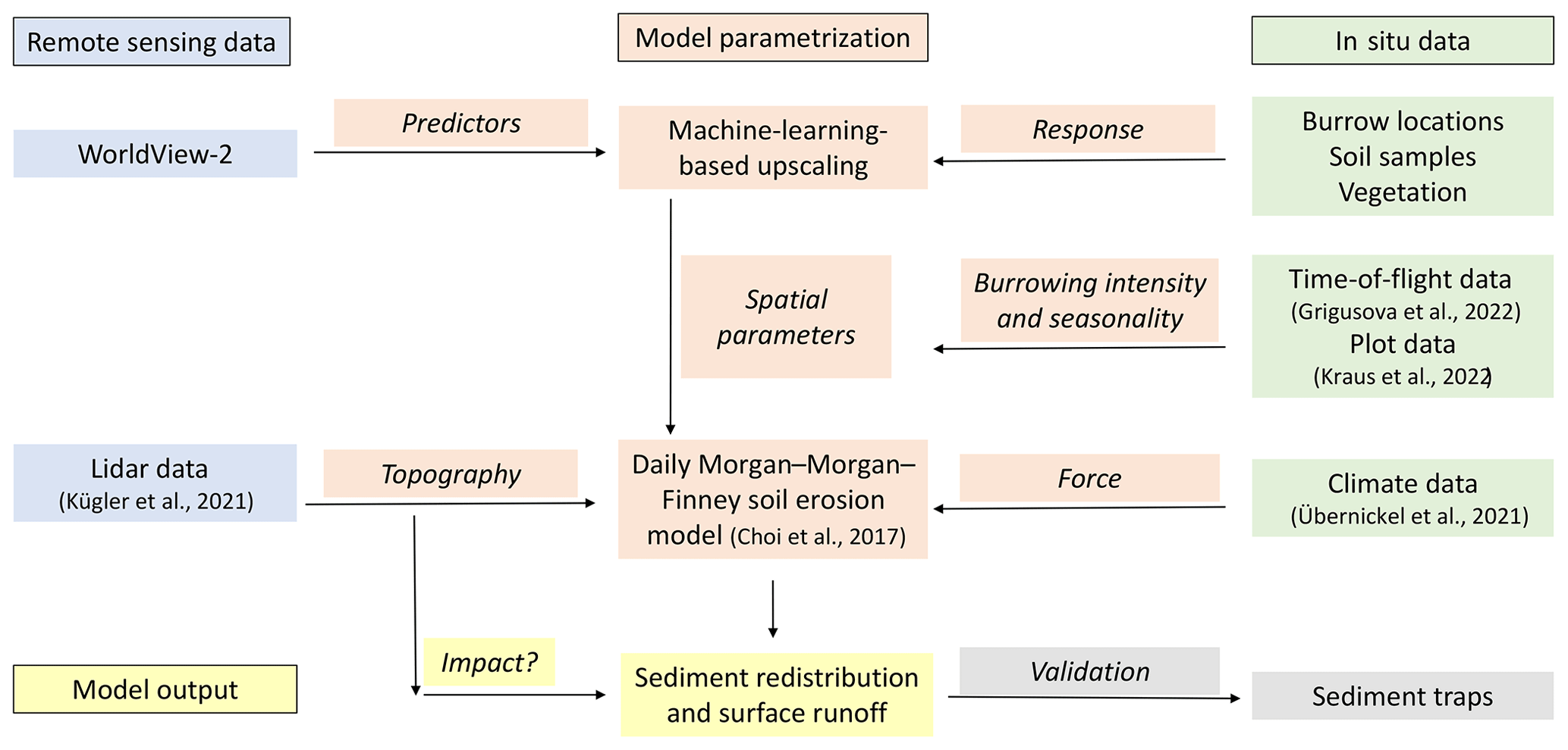
Figure 2 Flowchart of our study. Green indicates in situ input data; blue indicates remote sensing input data. Red indicates model parametrization. Yellow indicates model output and analysis. Gray indicates model validation.

3.1 In situ data

The study setup consisted of eight hillslope catchments: one north-facing and one south-facing hillslope catchment per study site. We defined a line with a width of 1 m from the top to the base of each hillslope catchment (see blue line, Fig. 1). We subdivided the track into tiles of 1 m². We saved the GPS information of each tile.

Within each tile of the line, we mapped burrow presence, land cover, and the extracted soil samples. A burrow consisted of an entrance and a mound (Fig. 3a). Each 1 m² tile with a burrow was described as a presence data point and tiles without a burrow as absence data points. We noted the size of the burrow, vegetation cover, and land cover types (bare soil, herbs, shrubs, trees) within the tile. We extracted 162 soil samples from soil without a mound at a depth of 10 cm. Additionally, we took a photo of the surface every second tile along the track.

To validate the model output, we set up sediment traps (Fig. 3b), with six traps per site, two of which were located at the hillslope catchment base and four were located on two random positions within the hillslope catchment. The sediment traps consisted of geotextile and wooden poles and had a length of 2–5 m. A total of 1.5 m of geotextile was laid horizontally down at the surface, and 1 m of geotextile was vertically attached to wooden poles to enable the collection of sediment (Fig. 3b).

The sediment accumulated within the traps was collected after 1 year, and its mass (cm³) and dry weight (kg) were estimated.

Climate information was retrieved from climate stations located adjacent to the hillslope catchments, which provide climate data in 5 min intervals (Übernickel et al., 2021). To force the model on an hourly basis, hourly air temperature, precipitation total and intensity, wind speed, wind direction, and humidity were calculated for the study period from 1 April 2016 to 1 December 2021. Evapotranspiration was estimated with the Penman–Monteith equation (Penman, 1948).

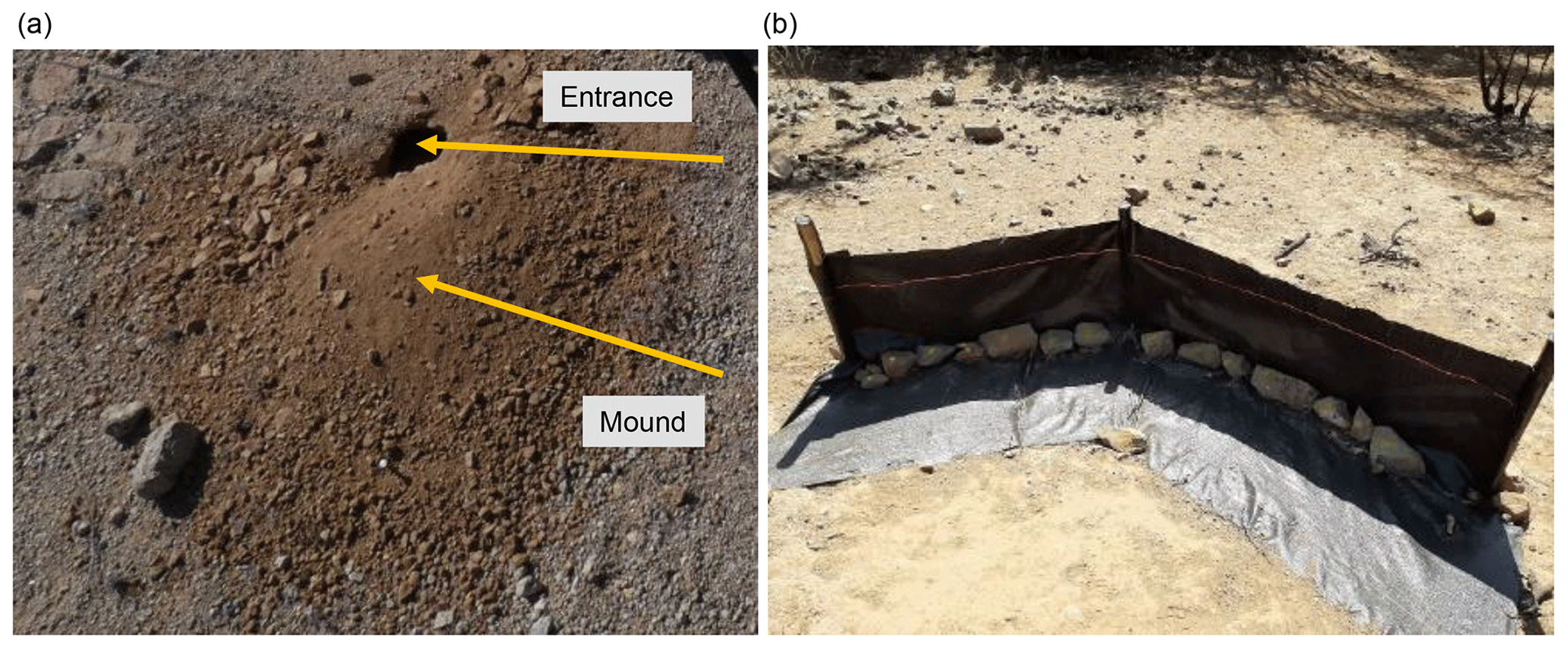
Figure 3 In situ constructions. (a) Example of a burrow consisting of burrow entrance and mound. (b) Fence construction used for the collection of eroded sediment to validate the model. Both photos by Paulina Grigusova.

3.2 Estimation of soil properties

We estimated several soil properties from the soil samples and photos collected in situ (Grigusova et al., 2022). We estimated the rock coverage on the surface and debris from the photos taken every second tile. For this, the photos were firstly classified into five classes. The classification was unsupervised using k means (Fig. A1). Then we calculated the ratio of pixels classified as skeleton and/or debris to the overall number of all pixels to determine the proportion of both parameters in percent.

In the lab, we estimated soil water content, bulk density, soil particle density, soil texture (sand; silt; clay; coarse, middle, and fine sand; coarse, middle, and fine silt), soil skeleton, organic matter, and organic carbon.

Gravimetric soil water content (%) (GSWC) described the mass of water within the soil sample and was estimated as in Eq. (1):

$$\begin{array}{}\text{(1)}& \mathrm{GSWC}={\displaystyle \frac{\left(S_{\mathrm{m}}-S_{\mathrm{d}}\right)}{S_{\mathrm{d}}}}\times \mathrm{100},\end{array}$$

where S_m (g) is the mass of moist soil measured directly after the extraction and S_d (g) is the mass of soil dried at 105 ^∘C for at least 24 h. Bulk density (g cm⁻³) (BD) was calculated as follows:

$$\begin{array}{}\text{(2)}& \mathrm{BD}={\displaystyle \frac{S_{\mathrm{d}}}{S_{\mathrm{v}}}},\end{array}$$

where S_v (cm⁻³) is the volume of the sample. Soil particle density (g cm⁻³) (SPD) was calculated as in Eq. (3):

$$\begin{array}{}\text{(3)}& \mathrm{SPD}={\displaystyle \frac{\mathrm{dm}}{S_{\mathrm{v}}}},\end{array}$$

where dm (g) is the dry mass of soil particles excluding pores.

Particle size distribution (%) of clay (< 0.002 mm); coarse, middle, and fine silt (0.002 to 0.02 mm); and coarse, middle, and fine sand (0.02 to 2 mm) was estimated according to Durner et al. (2017). Soil skeleton was estimated as the ratio of particles with a diameter above 2 mm. Ratio of organic matter (OM) was estimated as in Eq. (4):

$$\begin{array}{}\text{(4)}& \mathrm{OM}=\mathrm{1}-{\displaystyle \frac{S_c}{S_{\mathrm{d}}}},\end{array}$$

where S_c is the weight (g) of the sample dried at 500 ^∘C for 16 h.

We used pedotransfer functions to determine porosity, saturated soil moisture, hydraulic conductivity, water content at field capacity, and permanent wilting point. Pore ratio (θs) was estimated from bulk and particle density as in Eq. (5):

$$\begin{array}{}\text{(5)}& \mathit{\theta }s={\displaystyle \frac{\mathrm{BD}}{\mathrm{SPD}}}.\end{array}$$

Saturated water content (g g⁻¹) (W_s) was estimated as in Eq. (6):

$$\begin{array}{}\text{(6)}& W_{\mathrm{s}}=\mathit{\theta }s{\displaystyle \frac{p_{\mathrm{w}}}{\mathrm{BD}}},\end{array}$$

where p_w (g cm⁻³) is the density of water, which is set to be 1 g cm⁻³ (Pollacco, 2008).

Hydraulic conductivity Ks (m s⁻¹) was estimated as in Eq. (7):

$$\begin{array}{}\text{(7)}& Ks=\mathrm{1.15741}\times \mathrm{0.0000001}\times \exp \left(x\right),\end{array}$$

where x for sandy soil is

$$\begin{array}{}\text{(8)}& \begin{array}{rl}x& =\mathrm{9.5}-\mathrm{1.471}\times \left(\mathrm{BD}\times \mathrm{BD}\right)-\mathrm{0.688}\times \mathrm{OM}+\mathrm{0.0369}\\ & \times \left(\mathrm{OM}\times \mathrm{OM}\right)-\mathrm{0.332}\times \mathrm{CS},\end{array}\end{array}$$

and x for loamy and clayey soils is

$$\begin{array}{}\text{(9)}& \begin{array}{rl}x& =-\mathrm{43.1}+\mathrm{64.8}\times \mathrm{BD}-\mathrm{22.21}\times \left(\mathrm{BD}\times \mathrm{BD}\right)+\mathrm{7.02}\\ & \times \mathrm{OM}-\mathrm{0.1562}\times \left(\mathrm{OM}\times \mathrm{OM}\right)+\mathrm{0.985}\times \ln \left(\mathrm{OM}\right)\\ & -\mathrm{0.01332}\times C\times \mathrm{OM}-\mathrm{4.71}\times \mathrm{BD}\times \mathrm{CS},\end{array}\end{array}$$

where C is percentage of clay and CS is percentage of clay and silt (Wösten, 1997). To estimate water content at field capacity (%) (FC) and permanent wilting point (PWP), we applied functions by Tomasella et al. (2000) as these were developed for South American soils:

$$\begin{array}{}\text{(10)}& {\displaystyle }\mathrm{FC}=\mathrm{4.046}+\mathrm{0.426}\times \mathrm{Si}+\mathrm{0.404}\times C,\text{(11)}& {\displaystyle }\mathrm{PWP}=\mathrm{0.91}+\mathrm{0.15}\times \mathrm{Si}+\mathrm{0.396}\times C,\end{array}$$

where Si is the percentage of silt.

3.3 Processing of remote sensing data

The digital elevation models (DEMs) were calculated from the lidar data (Kügler et al., 2022; Horn, 1981) at a resolution of 0.5 m. Slope was calculated according to Horn (1981). Manning's surface roughness coefficient was estimated following Li and Zhang (2001). The topographic position index (TPI) and the topographic ruggedness index (TRI) were calculated according to Wilson et al. (2007). To calculate the TPI, the average elevation of pixels within a range specified by the user needs to be subtracted from the elevation of the central pixel. Positive values represent hills, while negative values represent valleys. The TRI adds together the elevation differences between a grid cell and its eight neighbors. It measures the relative level of topography irregularity: the higher the value, the more irregular the topography. Plan and profile curvature were determined after Zevenbergen and Thorne (1987). Connectivity indices, sinks, wetness index, flow direction, flow path, catchment slope, and catchment were calculated in SAGA GIS.

Single license stereo WorldView-2 images with a resolution of 0.5 m were retrieved from GAF AG Munich GmbH. The topographic correction of WorldView-2 images was done using the lidar data, solar elevation angle, solar zenith angle, and azimuth angle according to Goslee (2012). The digital surface models (DSMs) were calculated from the stereo images. Additionally, we extracted single bands and calculated the normalized difference vegetation index (NDVI).

3.4 The erosion model

3.4.1 Daily Morgan–Morgan–Finney model

The DMMF model is a combined soil erosion model used to estimate surface runoff and sediment flux on a field scale on a daily basis. Spatially, the DMMF model represents an area as several interconnected elements (e.g., pixels) of uniform topography, soil characteristics, land cover type, and vegetation structure. Through coupling, the model operates with flow direction algorithms: each element receives water and sediments from upslope elements and delivers the generated surface runoff and eroded soils to downslope elements. On a temporal scale, the model estimates surface runoff and sediment flux of each element on a daily basis. The model input parameters include climate, topography, soil properties, and land cover information (Choi et al., 2017). Data pre-processing, modeling, and analysis (see Fig. 2) were done in the R statistical environment. The raster data were cropped to the size of the hillslope catchments (Fig. 1). Input parameters are listed in Table 1 and plotted in Fig. A2.

During the model simulation, water and sediment are transferred from pixels located at higher elevations to pixels situated at lower elevations. This occurs in two stages: the first stage is the hydrological phase where the model calculates surface runoff, which happens when the amount of surface water input exceeds the water-holding capacity. The amount of surface runoff is computed by taking the infiltration capacity of the surface, the volume of surface water input, and the fraction of the impervious area of a pixel into account. Infiltration capacity represents the maximum amount of surface water that can penetrate the subsurface layer. It is determined by the percentage of the impervious area and the available pore space.

The second stage is the sediment phase, where the model estimates the sediment budget for each particle size class, based on the surface conditions. The model calculates the detachment and deposition of sediments in a step-by-step process. The sources of sediments are detached particles from the pixel itself due to rainfall and surface runoff and delivered soil particles from higher-elevation pixels. The detachment of soil particles by rainfall occurs when raindrops hit the ground with enough energy to detach soil particles from the surface. Rainfall has different impacts on areas with and without canopy cover, as canopy cover changes the kinetic energy of raindrops.

The quantity of soil particles detached by raindrops is calculated based on the soil particle detachability, the percentage of each particle size class, the bare soil surface area, and the kinetic energy of effective rainfall. The quantity of detached soil particles by surface runoff is calculated based on the soil particle detachability, the amount of runoff, the slope angle of the pixel, and the proportion of the bare surface area. The third source of sediment is from higher-elevation pixels and is averaged by the surface area of the pixel.

Once sediments are delivered to the surface runoff, a portion of the suspended sediments settle to the bottom due to gravitational force. To calculate this settling, the model requires the flow velocity of the runoff and the settling velocity of each particle size class, which are influenced by the flow depth, slope angle of the pixel, and Manning's roughness coefficient (Choi et al., 2019).

3.4.2 Estimation of spatial parameters

For spatial parameterization of the DMMF model, we predicted land cover, soil properties, and burrow distribution onto the hillslope catchments using machine learning techniques. We used the approach of Meyer et al. (2018). The most important predictors were selected by forward feature selection. The quality of the random forest (RF) models was assessed by leave-location-out cross-validation. We trained the model stepwise, using in situ data collected from seven of the hillslope catchments and validated the model using in situ data from the remaining hillslope catchment (Meyer et al., 2018). The prediction was done at 0.5 m spatial resolution. We used the WorldView-2 layers obtained with a single license with GAF, NDVI, DEM, DSM, slope, and roughness as predictors. The PAN-sharpening of the WV-2 layers was done by GAF. The accuracy of the classifications was estimated by dividing the number of correctly classified pixels to the number of all pixels.

For the area-wide prediction of burrow locations across the hillslope catchments, we used the burrow presence and absence data (Sect. 3.1) as the response data within the RF models. The accuracy was 0.82 for PdA, 0.77 for SG, 0.75 for LC, and 0.85 for NA. The prediction of soil properties was done using soil properties estimated along the track line (see Sect. 3.1) as response data within the RF models. All of the models reached a high accuracy (see Table A1).

To obtain land cover classification, we used, as the response within the RF models, the land cover measured in situ. The classes were soil without rocks, rocks, biocrusts, grass/herbs, shrubs, and trees. Predictor values for each class were extracted from at least 100 polygons per site and class. The accuracy of the RF models was 0.71 for PdA, 0.81 for SG, 0.83 for LC, and 0.75 for NA.

The vegetation height measured in plots was averaged for each class per site. All pixels classified as the respective class were assigned the same vegetation height information. Vegetation density was estimated per hillslope catchment as the number of vegetation individuals per square meter. Vegetation diversity was calculated with the Shannon index (Shannon, 1948). The interception area was the area not covered by vegetation (herbs, shrubs, or trees).

3.4.3 Inclusion of bioturbation

In the grid cells with predicted burrow locations, we adapted the values of input parameters to include bioturbation. The adaptations varied with climate zone and burrow size. The size, geometric structure, and excavation rates of burrowing animals were previously estimated at a high spatial and temporal resolution (Grigusova et al., 2022). Based on these results, we firstly adjusted the microtopography. We modified the layer depth to represent burrow entrance and elevation to represent animal mound. Mounds were always located downslope of burrow entrances in the direction of flow.

Secondly, we adjusted the soil properties. The soil properties texture and organic carbon were estimated from soil extracted from mounds in Kraus et al. (2022). In this study we additionally estimated bulk density, initial water content, soil skeleton, porosity, saturated water content, available water capacity, and water content at field capacity from the same dataset (see Sect. 3.2). We calculated the median value of each property for the samples extracted from mounds and for the samples extracted from soil without mounds. Then, we estimated the change in percent between these two values. This was then used to adjust the soil property for each pixel including a mound.

Thirdly, modeled mound pixels had to be cleared from ground vegetation cover. For this, we removed ground vegetation cover from pixels with burrow locations and decreased ground vegetation cover, height, diameter, and number of ground vegetation individuals from adjacent pixels as measured in situ. Then, the number of rocks and amount of debris were set as estimated from soil samples (Sect. 3.2)

Animal activity has been found to be highly variable throughout the year (Grigusova et al., 2022; Kraus et al., 2022). The density of burrows does not stay stable throughout the year but increases or decreases depending on the season and climate zone. We therefore artificially removed or added burrows into the hillslope catchments during the particular seasons. For this, we adapted the density of soil, the topography, and vegetation cover accordingly. We created a 3D model of the burrow structure and adjusted subsurface soil properties and properties of soil excavated to the surface: the removed vegetation within the pixel with a predicted burrow and decreased adjacent vegetation cover.

Lastly, we also included the vertical movement of sediment particles from deeper soil layers to the surface depending on climate. Animals were found to reconstruct their burrows after each rainfall event (Grigusova et al., 2022). Corresponding with these findings, we increased the entrance depth and mound height by 30 % after each rainfall event, which represents the averaged value found in the previous study (Grigusova et al., 2022).

For the validation, we ran the model for the time periods between the installation of sediment fences and the collections of sediment. We compared the mass and weight of modeled and collected sediment and estimated R² and RMSE. To test the importance of the inclusion of individual bioturbation parameters into the model, we ran the model under four conditions: (i) no burrows, (ii) solely entrances, (iii) solely mounds, and (iv) entire burrows (entrances and mounds).

Table 1 Model input layers and respective changes to layer values at the predicted burrow locations. Ground vegetation was removed from the respective pixels, while tree canopy was not changed. The values were estimated as described in Sect. 3.5.2. Using the adjusted values, we calculated evapotranspiration using the Penman–Monteith equation, surface roughness from the elevation layer, hydraulic conductivity, water content at field capacity, and saturated water content using pedotransfer functions.

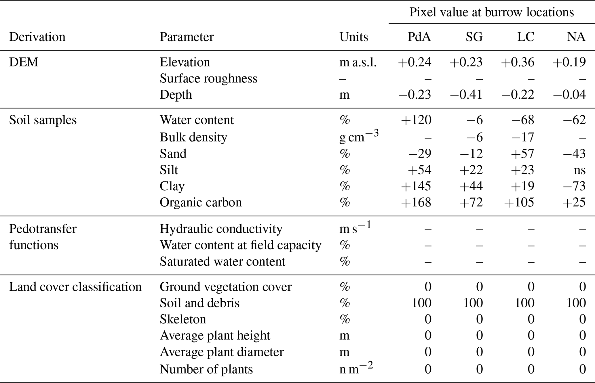
The ns means not significant.

3.5 DMMF model sensitivity test

We conducted a sensitivity test to identify those input parameters which significantly influence the model output. For this, we first estimated the mean value of each input parameter. Then, we created an artificial hillslope catchment of 100 m × 100 m. To start the test, each pixel received the mean value of each parameter. We ran the model for one rainfall event. Then, stepwise, we changed the single input parameter values from their minimum to their maximum values while not adjusting any other parameters. To quantify the significance of the input variations, we conducted a t test (Table A2). For this, we compared the amount of redistributed sediment of each model run to the first model run.

3.6 Impact of burrows on surface processes

We estimated burrow density as the ratio of pixels with predicted burrows to all pixels. Additionally, we calculated the ratio of pixels which are part of a burrow aggregation to all pixels which include a burrow. Burrow aggregation describes at least four neighboring pixels with predicted burrows. We calculated the amount of excavated sediment as a sum of burrow density and the burrow excavation rate as estimated in Grigusova et al. (2022).

To estimate the impact of burrows on sediment redistribution and surface runoff, we ran the DMMF model for the time period from 1 April 2016 to 31 December 2021 for all hillslope catchments. We ran the model (i) with no burrows and (ii) with entire burrows. We estimated (i) sediment redistribution (accumulation minus erosion) and (ii) surface runoff. We analyzed the redistribution and runoff on the plot (1 m²) and hillslope catchment (1 ha) scale.

Lastly, to analyze under which biotic and abiotic environmental parameters (topography, vegetation cover) the bioturbation enhances sediment erosion or accumulation, we set up a generalized additive model (GAM) (Wood, 2006). For this, we first subtracted the output of the model with no burrows from the output of the model with entire burrows. Within each pixel, two processes are happening simultaneously: a certain amount of sediment erodes, and a certain amount of sediment accumulates. To estimate the sediment redistribution for each pixel of each model run, we estimate which of these processes dominated. Positive pixel values thus mean that bioturbation enhanced sediment accumulation; negative pixel values mean that bioturbation enhanced sediment erosion. We tested the following environmental parameters: mound density, vegetation cover, elevation, slope, aspect, TRI, TPI, curvature and connectivity, and wetness index. The model performance was evaluated by the percentage of explained data variance. We analyzed the impact of environmental parameters within 1 m and within 10 m from the burrows.

4 Results

4.1 Model sensitivity test and accuracy

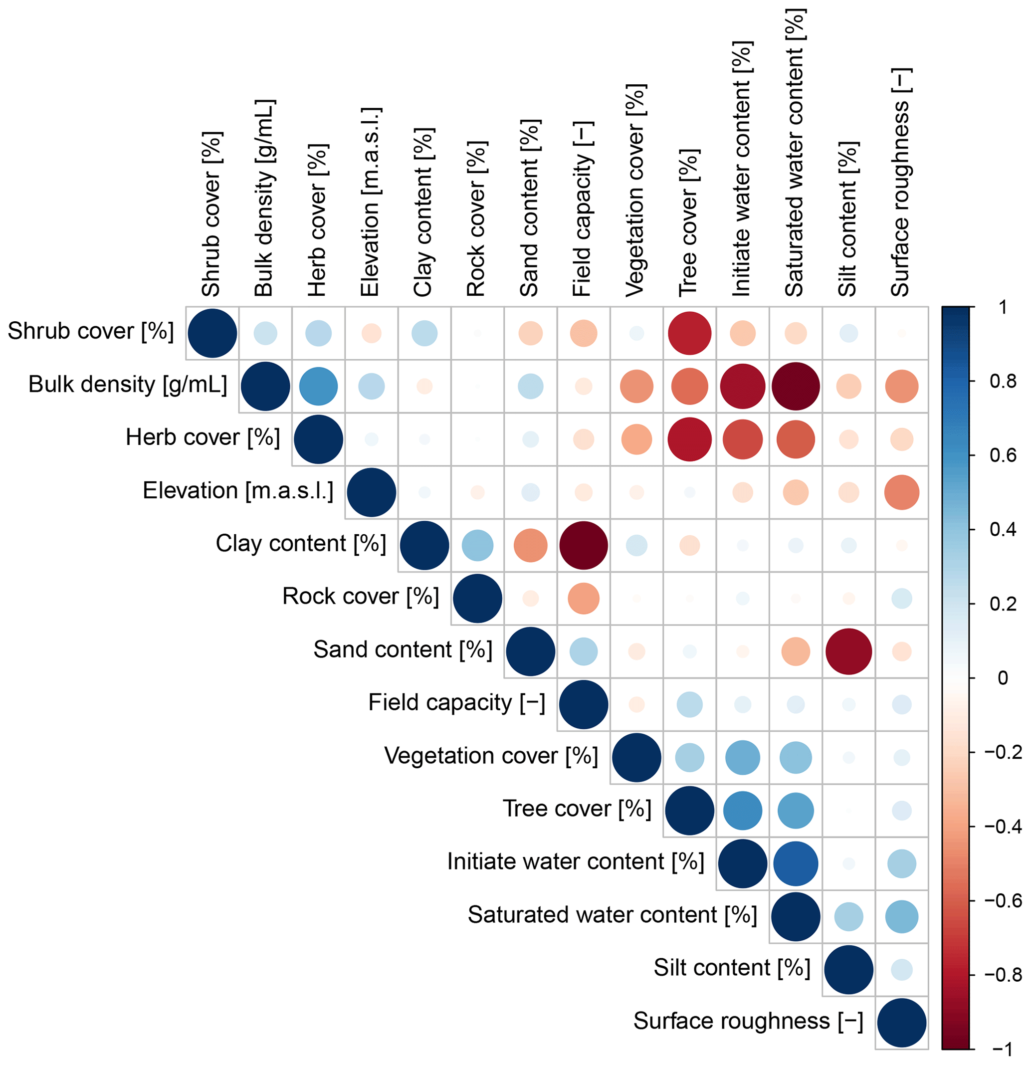
Parameters which significantly influenced the model output were precipitation, slope, vegetation cover, surface roughness, silt content, and water content (Table A2). There was a correlation between some of the spatial model parameters (Fig. A10), especially between the initial and saturated water content, between water content and vegetation cover, and between clay content and field capacity. However, a high correlation between spatial parameters does not mean that these parameters impact the sediment redistribution in a similar way.

We quantified the model performance by comparing the modeled and measured sediment redistribution. The performance varied depending on the burrow inclusion (Figs. 4 and 5). The performance of the model without any bioturbation was lower (R²= 0.73, RMSE = 1.50, MSE = 2.27), as when burrow entrances (R²= 0.81, RMSE = 1.34, MSE = 1.16) or mounds (R²= 0.83, RMSE = 1.10, MSE = 1.22) were included. The model had the highest performance when entire burrows were included (R²= 0.85, RMSE = 1.01, MSE = 1.01). However, as the scatterplots showed, the model performance seemed to be determined strongly by one measurement (Fig. 5). For this reason, we calculated the metrics without this measurement (Fig. A2). The model without any burrows (R²= 0.17, RMSE = 1.18, MSE = 1.39) in this case performed much lower than models with burrows. The model performance increased when burrow entrances (R² = 0.48, RMSE = 0.61, MSE = 0.78) or mounds (R²= 0.51, RMSE = 0.75, MSE = 0.57) were included. The model with whole burrows reached the highest performance (R²= 0.71, RMSE = 0.63, MSE = 0.39). When we compare the modeled redistribution to the sediment redistribution estimated using time-of-flight cameras in Grigusova et al., (2022), the differences appear to be minor (R²= 0.62, RMSE = 0.12, MSE = 0.35).

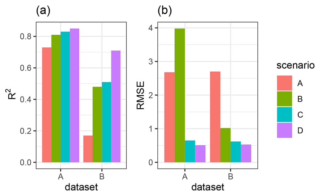
Figure 4 R² and RMSE of the Morgan–Morgan–Finney soil erosion model. For dataset A, we compared the amount of sediment collected in all sediment fences with the modeled eroded sediment (see Fig. A3). For dataset B, we removed one measurement, as the R² seemed to be defined by this measurement (see Fig. A4). For scenario A, we did not include any burrows into the model. For scenario B, we included burrow entrances, and for scenario C, we included mounds. For scenario D, we included whole burrows into the model. The adjustments made to include entrances, mounds, and burrows into the model are described in Sect. 3.5.2.

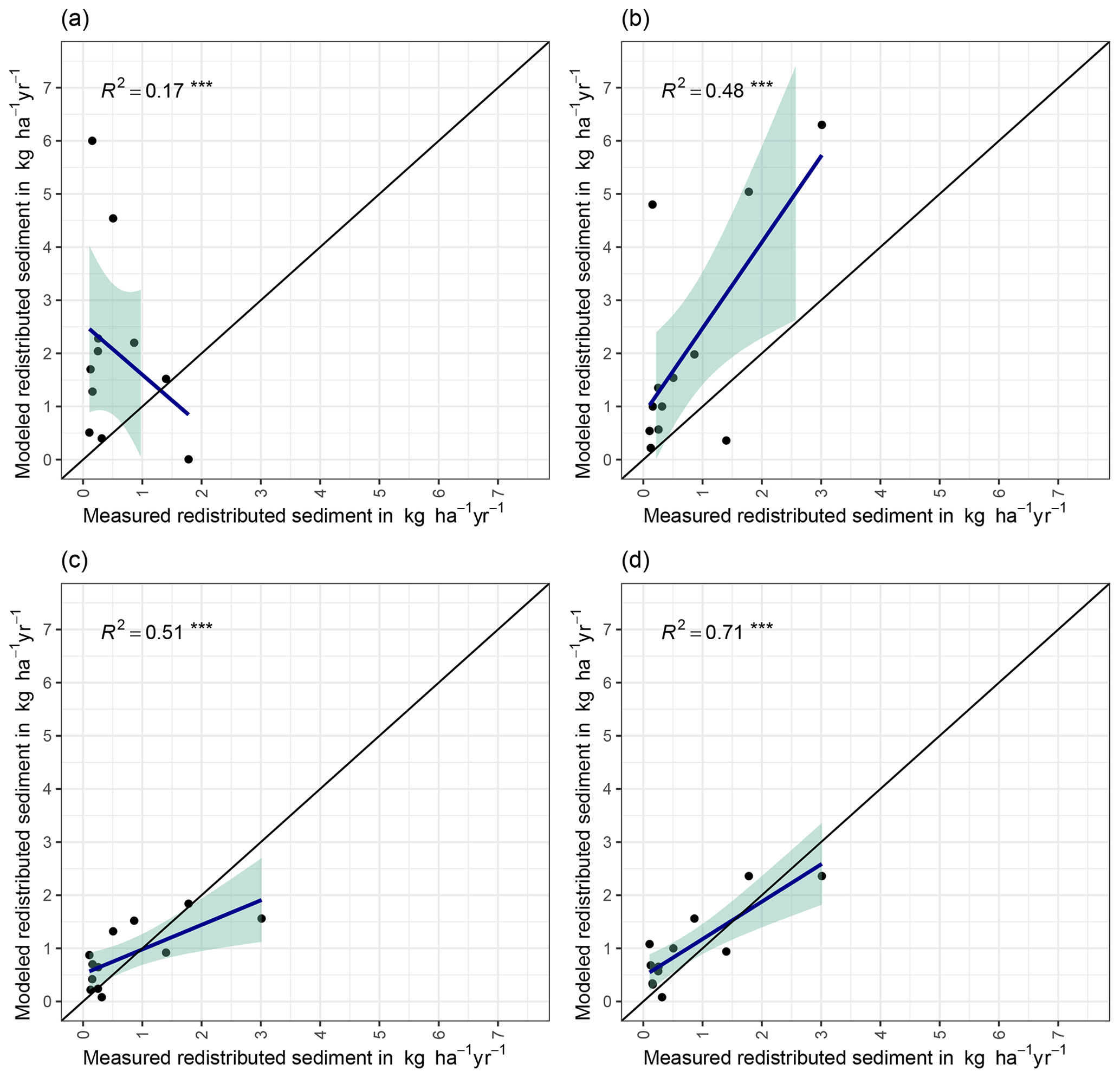
Figure 5 Measured and modeled redistributed sediment without an outlier. (a) Model without bioturbation. (b) Model with entrances. (c) Model with mounds. (d) Model with burrows.

4.2 Model output: surface runoff and sediment redistribution

Hillslope catchment-wide sediment redistribution (1 ha resolution) was the highest in humid NA, followed by Mediterranean LC, semi-arid SG, and arid PdA (Figs. 6a, b, 8). In NA, LC, and SG, the erosion processes dominated, while in PdA, more sediment accumulated than eroded. The impact of burrows on sediment redistribution was significant in arid PdA, semi-arid SG, and Mediterranean LC. Burrows increased sediment redistribution by 137.8 % ± 16.4 % in arid PdA (3.53 kg ha⁻¹ yr⁻¹ vs. 48.79 kg ha⁻¹ yr⁻¹), by 6.5 % ± 0.7 % in semi-arid SG (129.16 kg ha⁻¹ yr⁻¹ vs. 122.05 kg ha⁻¹ yr⁻¹), and by 15.6 % ± 0.3 % in Mediterranean LC (4602.69 kg ha⁻¹ yr⁻¹ vs. 3980.96 kg ha⁻¹ yr⁻¹). Overall, bioturbation increased sediment accumulation in the arid zone (as the magnitude of the sediment excavation by the animals exceeded sediment erosion which occurs during rainfall events), but it increased sediment erosion in semi-arid and Mediterranean climate (where animal burrowing activity and rainfall are present). The largest impact was found under Mediterranean conditions. We found no significant effect on redistribution in the humid zone (Fig. 7). However, impact of bioturbation varied throughout the hillslope catchment (Figs. 7, 8, and 9).

Surface runoff was the highest in humid NA, followed by Mediterranean LC, arid PdA, and semi-arid SG (Fig. 6c). The impact of burrows on surface runoff was significant in all climate zones. Burrows increased surface runoff in PdA by 34 %, in SG by 40%, and in LC by 4.1 %, but it decreased surface runoff by 5.9 % in NA. Hillslope catchment-wide maps are shown in Figs. A6–A8.

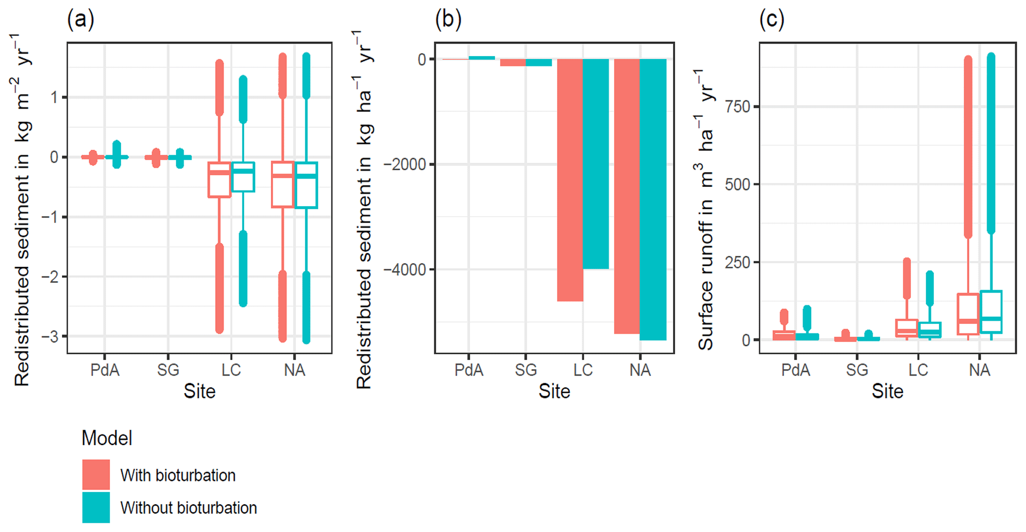
Figure 6 Summary of model outputs across the climate gradient. PdA is arid Pan de Azúcar. SG is semi-arid Santa Gracia. LC is Mediterranean La Campana. NA is humid Nahuelbuta. Graphs (a) and (b) show the modeled sediment redistribution. Positive values indicate sediment accumulation; negative values indicate sediment erosion. In (a) sediment redistribution is shown on a pixel scale (in kg m⁻² yr⁻¹), while in (b) sediment redistribution is shown on the hillslope catchment scale (in kg ha⁻¹ yr⁻¹). The impact of bioturbation on sediment redistribution was estimated by a t test and was significant in three sites: PdA${}^{***}$, SG${}^{**}$, and LC${}^{***}$. Bioturbation increased sediment redistribution by 137.8 % in PdA, by 6.5 % in SG, and by 15.6 % in LC. For hillslope catchment-wide maps see Figs. A6–A8. Graph (c) represents the modeled surface runoff on the hillslope catchment scale (in m³ ha⁻¹ yr⁻¹). The impact of bioturbation on surface runoff was estimated by a t test and was significant at all sites. Bioturbation increased surface runoff in PdA by 34 %, in SG by 40 %, and in LC by 4.1 %, but it decreased surface runoff by 5.9 % in NA. For hillslope catchment-wide maps, see Fig. A6.

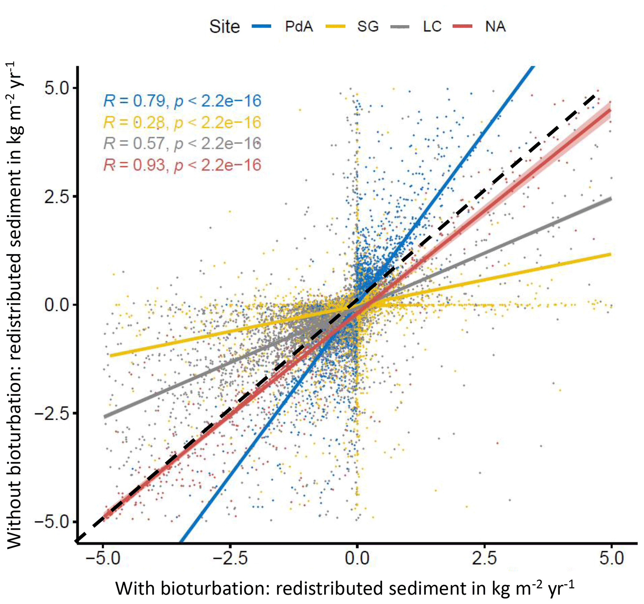
Figure 7 Comparison of the model outputs with and without bioturbation of each pixel (0.5 m) in all study sites. The x axis shows the output of the model with bioturbation, and the y axis shows the model output without bioturbation. PdA is arid Pan de Azúcar. SG is semi-arid Santa Gracia. LC is Mediterranean La Campana. NA is humid Nahuelbuta. Points represent single pixel values; lines show linear regressions for the sites. The lower the R, the higher the impact of burrows is on sediment redistribution at the resolution of 0.5 m. The dashed black line symbolizes a perfect correlation – along this line the bioturbation would have no effect on sediment redistribution. Bioturbation leads to more accumulation if the regression line representing results from a particular climate zone is steeper than the perfect correlation line. Bioturbation leads to more erosion if the regression line representing results from a particular climate zone is flatter than the perfect correlation line. Bioturbation increases sediment accumulation in arid PdA (through the high burrowing rate, more sediment is accumulated on the surface than eroded during rainfall events). Bioturbation increases sediment erosion in semi-arid SG and Mediterranean LC. In absolute terms, the highest impact on sediment redistribution is in the Mediterranean climate zone. The lowest impact is in the humid zone.

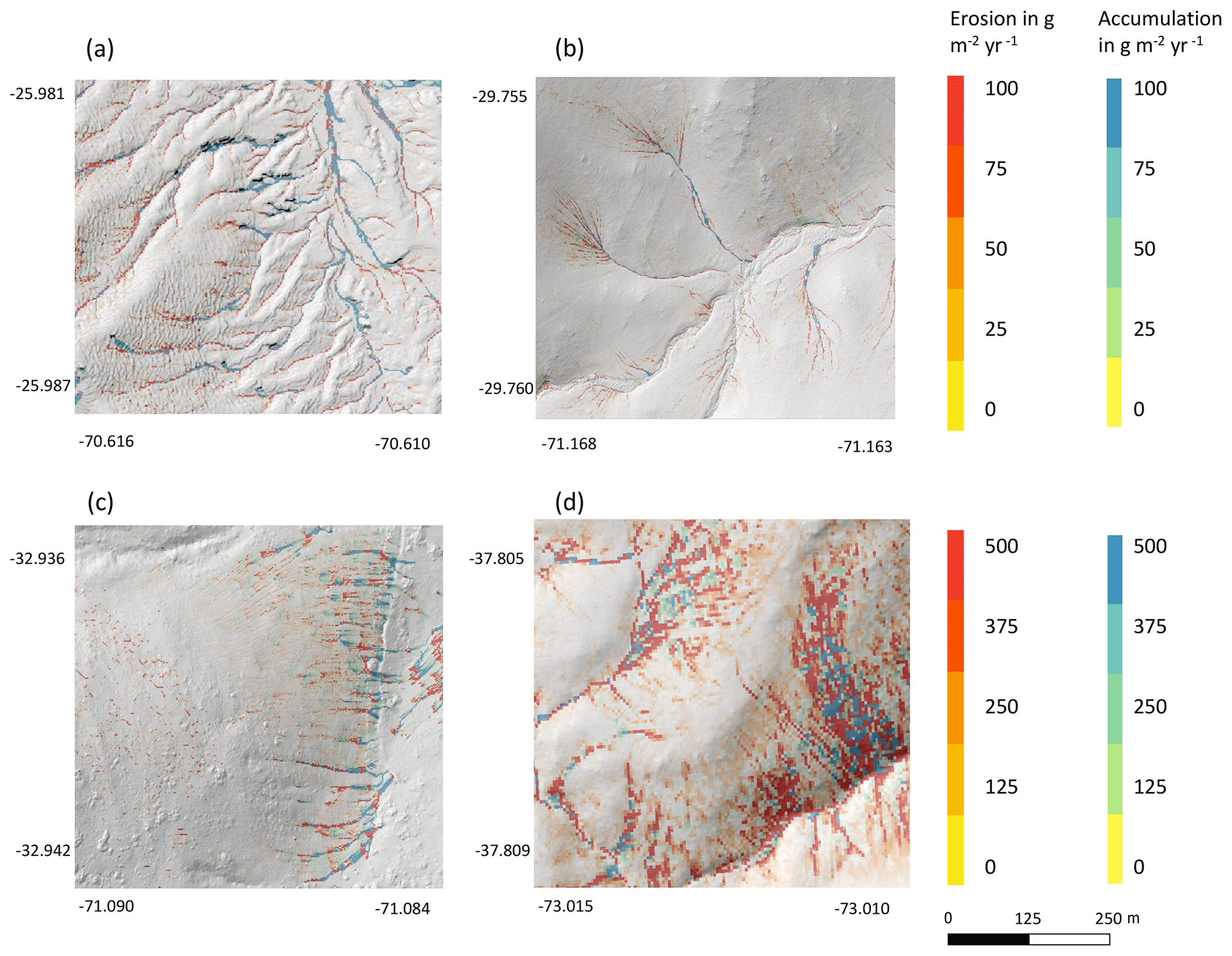
Figure 8 Hillslope catchment-wide predicted sediment redistribution. Colors indicate sediment redistribution. Gray indicates the hill shading calculated from lidar data. (a) Pan de Azúcar, (b) Santa Gracia, (c) La Campana, and (d) Nahuelbuta.

4.3 Role of continuous burrowing activity on sediment redistribution

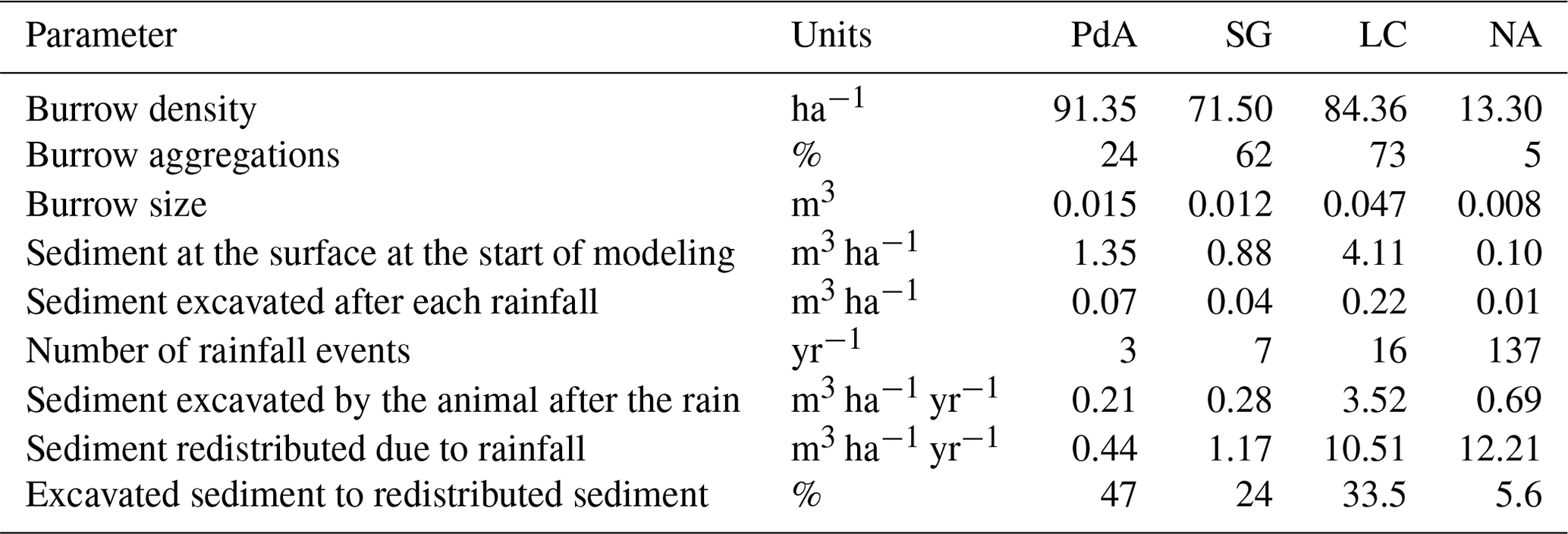
We included transport of the sediment to the surface by animal excavation into the model. The density of burrows was the highest in the arid PdA, then Mediterranean LC, and then semi-arid SG, and it was the lowest in humid NA. Burrows were mostly distributed within groups of several burrows in Mediterranean LC and semi-arid SG, while they were more evenly distributed in the arid PdA and humid NA. The burrows were of the largest in Mediterranean LC, followed by arid PdA, semi-arid SG, and humid NA. Similarly, the highest volume of excavated sediment at the beginning of the modeling period was in Mediterranean LC and arid PdA. The volume of excavated sediment during the burrow reconstruction after rainfall events was the highest in humid NA, followed by Mediterranean LC, semi-arid SG, and arid PdA. The percentage of sediment excavated by the animal to sediment redistributed during rainfall events was 128 % in PdA, 24 % in SG, 33.5 % in LC, and 5.6 % in NA.

Table 2 Impact of animal bioturbation activity on overall sediment redistribution on various scales. The bioturbation activity was estimated using time-of-flight-based cameras in Grigusova et al. (2022). This study showed that animals reconstruct their burrows after each rainfall event. During this process, 10 % of the overall sediment burrow volume is relocated from within the burrow to the surface. We integrated this process into our model and calculated the percentage of newly excavated sediment by the animals to the amount of sediment which was redistributed during rainfall for the period of 1 year.

4.4 Role of adjacent environment

We subtracted the output of the model with included burrows from the output of the model without burrows (Fig. A8). Although the burrows on average enhanced sediment erosion on the hillslope catchment scale, the high-resolution maps unveiled that burrows enhance sediment erosion within some pixels, while they rather increased sediment accumulation within others.

The amount of data variance explained by the GAM models (see Sect. 3.6.) differed between models (Table A3). Models estimating the impact of environmental parameters on sediment redistribution within 1 m from the burrows explained 3.84 % of the variance in PdA, 37.1 % in SG, 46 % in LC, and 42. % in NA. Models estimating the impact of environmental parameters on sediment redistribution within 10 m from the burrows explained 1.99 % of the variance in PdA, 12.8 % in SG, 52 % in LC, and 72.9 % in NA. The parameters selected for SG were slope, roughness, curvature, TRI, and NDVI. Parameters selected for LC were elevation, slope, NDVI, sinks, and roughness. Parameters selected for NA were elevation, slope, aspect, TRI, sinks, and roughness (Fig. 10).

Bioturbation strongly increased sediment redistribution (erosion and accumulation) at high values of elevation, slope, surface roughness, TRI, sinks, and topographic wetness index; at the middle values of elevation and aspect; and at low values of profile curvature and NDVI. From these parameters, bioturbation increased sediment erosion at high and middle values of elevation; at high values of slope, sinks, and TRI; and at low values of profile curvature. Bioturbation increased sediment accumulation at high values of surface roughness and topographic wetness index and at low values of NDVI (Figs. A3–A8).

Bioturbation somewhat enhanced sediment erosion at medium values of surface roughness, NDVI, and sinks and at low values of topographic wetness index. Bioturbation somewhat increased sediment accumulation at low values of slope and TRI, at low and medium values of elevation, and at high values of profile curvature.

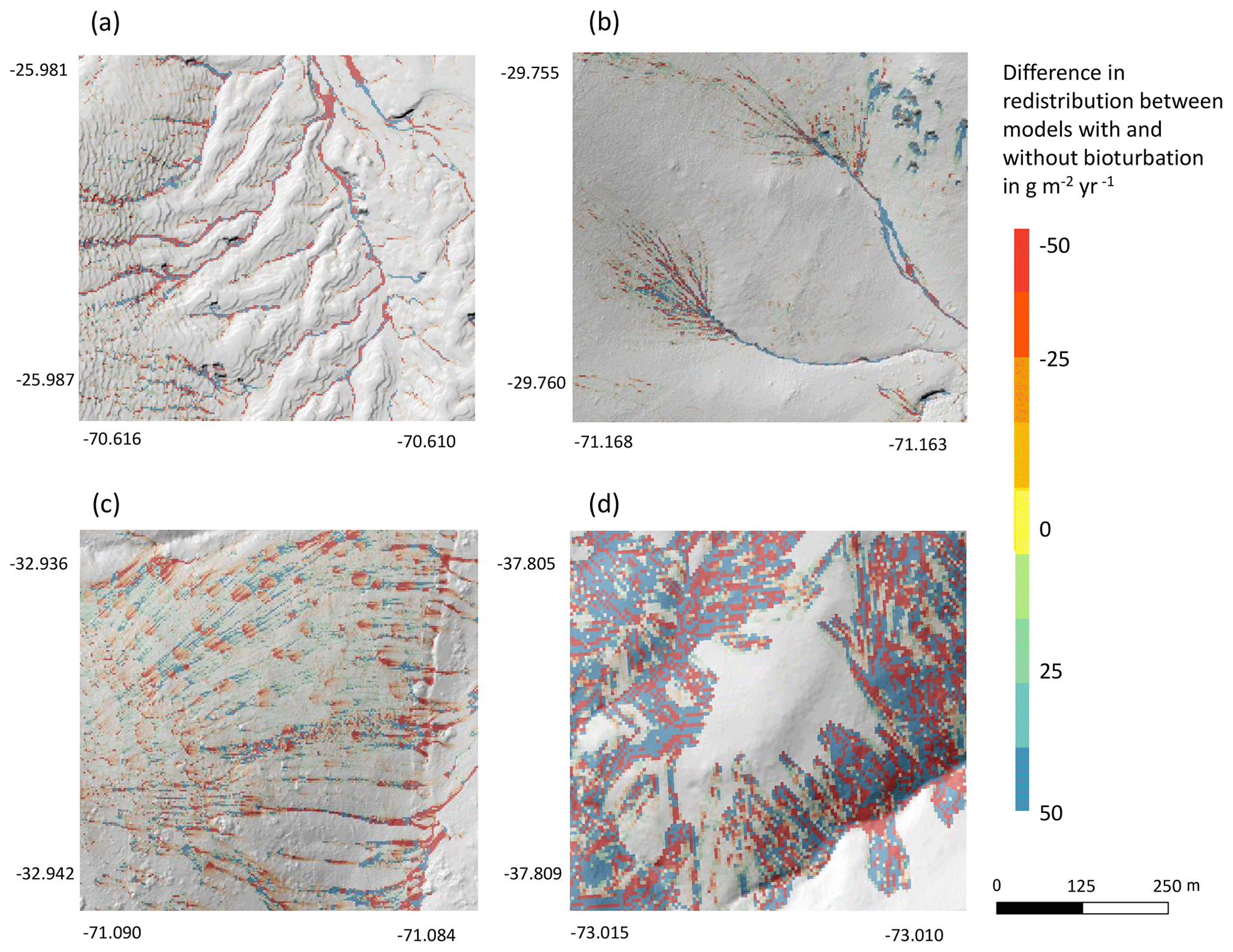
Figure 9 Hillslope catchment-wide impact of bioturbation on sediment redistribution. Color indicates the impact. Positive values indicate that bioturbation enhanced sediment accumulation; negative values indicate that bioturbation enhanced sediment erosion. Gray indicates the hill shading calculated from lidar data. (a) Pan de Azúcar, (b) Santa Gracia, (c) La Campana, and (d) Nahuelbuta.

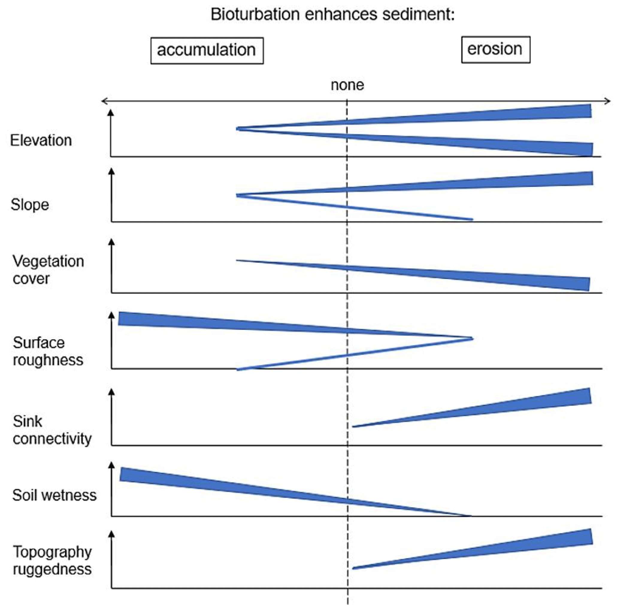
Figure 10 This figure is a conceptual summary of the detailed results from Figs. A3–A8. Bioturbation increases erosion or accumulation depending on the values of environmental parameters. The dependencies are the same for all climate zones. The figure is the conceptual summary for all climate zones; therefore, there are no values stated on the x and y axes. The x axis shows whether bioturbation increases erosion or accumulation. The y axes are environmental parameters. Line thicknesses indicate the magnitude of impact. Please note that bioturbation has no impact on sediment redistribution in regions with low sink connectivity and topographic ruggedness. The relationship between the values of environmental parameters and the impact of bioturbation is not linear: bioturbation can have the same impact on sediment redistribution at high or low values of an environmental parameter but a contrasting impact at middle values of this parameter (as in this case for elevation, slope, or surface roughness).

5 Discussion

5.1 The inclusion of bioturbation increases model performance

Overall, our DMMF model including bioturbation performed much better than the model without bioturbation. The DMMF model without bioturbation performed worse (RMSE of 1.18 kg ha⁻¹ yr⁻¹ and R² of 0.17) than the model with bioturbation (RMSE was 0.63 kg ha⁻¹ yr⁻¹ and R² was 0.71).

We hence argue that the higher accuracy of our model can be explained with the inclusion of bioturbation. This is confirmed by the fact that our model run without bioturbation performed similarly to previously run models without bioturbation: in earlier studies, the accuracy of the MMF model reached an RMSE between 4.9 and 8.2 kg ha⁻¹ yr⁻¹, with an estimated R² of between 0.21 and 0.57 (Jong et al., 1999; Vigiak et al., 2005; López-Vicente et al., 2008; Vieira et al., 2014; Choi et al., 2017). However, we acknowledge that previous studies were all conducted in more temperate climate zones. To be able to compare our results with previous studies, we calculated the model performance considering solely the Mediterranean and humid climate zone, which are more similar in climate to the more temperate locations of previous studies. The performance of the model was still high (R²= 0.72, RMSE = 0.45 kg ha⁻¹ yr⁻¹), confirming the conclusion that bioturbation increased model performance.

We compared the modeled impact of bioturbation on sediment redistribution with the impact of bioturbation estimated in previous studies. In the humid zone, our model predicted an erosion up to 3.5 kg m⁻² yr⁻¹. This estimation is in line with erosion rates established by in situ measurements in other studies conducted in a more humid climate zone (between 1.5 and 3.7 kg m⁻² yr⁻¹) (Black and Montgomery, 1991; Yoo and Mudd, 2008; Yoo et al., 2005; Rutin, 1996). This also confirms the reliability of our approach. Previous authors estimated the impacts using rainfall simulators, erosion pins, or splash boards. The measurements were conducted for a time period between 3 months and 3 years, and the sites were revisited for each estimation. We do not compare our results with studies which previously applied models to estimate impacts of bioturbation, as, to our knowledge, none of the previous studies integrated vertebrate burrow structures into a soil erosion model and ran the model on a daily basis.

5.2 The relevance of bioturbation for sediment redistribution depends on the environmental context

On the hillslope catchment scale (1 ha), our study finds that bioturbation increases erosion in semi-arid and Mediterranean zone, increases accumulation in the arid zone, and has no impact within the humid zone (Fig. 6b). In contrast, bioturbation increases both erosion and accumulation on the plot scale (1 m²) (Fig. 6a). On this scale, in the arid and semi-arid zone, sediment erosion and accumulation were predicted to be about equal (erosion and accumulation both up to 0.1 kg m⁻² yr⁻¹ in the arid zone and erosion and accumulation both up to 0.2 kg m⁻² yr⁻¹ in the semi-arid zone; see Fig. 6a). Bioturbation marginally increased erosion and decreased accumulation in the semi-arid zone but reduced accumulation 2-fold in the arid zone. In contrast, in the Mediterranean and humid zone, erosion was predicted to be almost double when compared to accumulation (predicted erosion up to 2.5 kg m⁻² yr⁻¹ and accumulation up to 1.4 kg m⁻² yr⁻¹). Inclusion of bioturbation increased erosion up to 3 kg m⁻² yr${}^{-\mathrm{1},}$ and accumulation up to 1.6 kg m⁻² yr⁻¹ in the Mediterranean zone, while it had no significant effect in the humid zone. We argue that sediment redistribution due to bioturbation is heavily influenced by mesotopographic structures which determine the flow path of surface runoff and influence the infiltration processes. Due to this, the erosion and accumulation on the plots scale are more heavily impacted by bioturbation with increasing surface runoff.

Our study found an increase of erosion in the semi-arid and Mediterranean climate zone to be between 6.5 % and 15.6 % due to bioturbation. Previous studies found that even a small increase of erosion has significant impacts on the whole hillslope catchment. A 10 % increase in erosion rates over a 10-year period can lead to significant changes in the landscape, including, for example, a 20 %–30 % reduction in soil thickness and an increase in sediment transport in nearby rivers (Kuhn, 2016).

According to our analysis, bioturbation increases erosion or accumulation of sediment mostly based on an interplay between topographic structures elevation, slope, and TRI (Fig. 10). Over all research sites, this study found that bioturbation leads to an increase in surface erosion in areas where erosional processes dominate (upper and/or steeper slopes) and tends to increase sediment accumulation in areas where sediment is naturally deposited (e.g., lower slopes or shallow depressions; Fig. 10). This finding is based on the fact that erosion in general is positively affected by slope and negatively by surface roughness and vegetation (Rodríguez-Caballero et al., 2012; Wang et al., 2013; Kirols et al., 2015). Additionally, the redistribution of sediment is largely affected by topographic meso-/macroforms, such as rills or cliffs. These can be quantified by topographic ruggedness index (TRI), which describes the amount of elevation drop between adjusting cells of DEM (Wilson et al., 2007). At high values of this index, we would therefore expect high erosion rates, due to concentrated runoff within the connected rills or undisturbed flow of runoff from the cliffs downslope.

Our data show that one burrow provides up to 0.43 m³ of additional loose sediment at the surface (Table 2), while the surface roughness increases up to 200 % (Grigusova et al., 2022). When including burrows into the model, with slope values from 0 to 5^∘, the presence of burrows had no impact on sediment redistribution. From 5^∘ onwards it increased sediment erosion proportionally to the slope of the hillside (an increased erosion from 0.4 g ha⁻¹ yr⁻¹ in the semi-arid zone to 150 kg ha⁻¹ yr⁻¹ in the Mediterranean zone; Figs. A3–A6). Similarly, at locations with elevation drops ranging from 0 m to 0.2 m (lower TRI values), the presence of burrows had no impact. However, at locations with elevation drops of 0.2 to 0.5 m (higher TRI values), bioturbation increases sediment erosion by 1.5 kg ha⁻¹ yr⁻¹ (Figs. A3–A8). Lastly, bioturbation proportionally increased accumulation when the surface roughness values were above 0.5 (an increased accumulation from 0.2 g ha⁻¹ yr⁻¹ in semi-arid zone to 5000 kg ha⁻¹ yr⁻¹ in the Mediterranean zone; Figs. A3–A6).

We conclude that, in locations with slope values over 5^∘ or at locations with sudden drops in elevation (high TRI) and connected rills, more sediment is eroding than accumulating. Here, additional surface sediments generated by bioturbators provide more source material for erosion, and thus bioturbation increases sediment erosion at these locations (Figs. 10 and 11). In contrast, at locations with a slope below 5^∘, where processes are dominantly controlled by surface roughness, sediment accumulation caused by bioturbation increases proportionally when the surface roughness has a value above 0.5. This is likely because burrows through their above-ground structures heavily increase surface roughness (Grigusova et al., 2022), and hence the presence of bioturbating animals leads to an increase in sediment accumulation.

Additionally, we hypothesize that it is not only the additional availability of sediment on the surface and the topography of the vicinity which controls the contribution of bioturbation to sediment surface flux, but also the spatial distribution of animal burrows. We interpret that, in locations with high burrow aggregation, surface flow might be redirected and centralized around the aggregates and thus increase sediment erosion in the areas adjacent burrow aggregates (Fig. 11). This mechanism could explain why bioturbation promotes sediment erosion especially in the Mediterranean zone, where burrows are more aggregated. The relative role of burrow aggregation should be studied in detail and included in future studies.

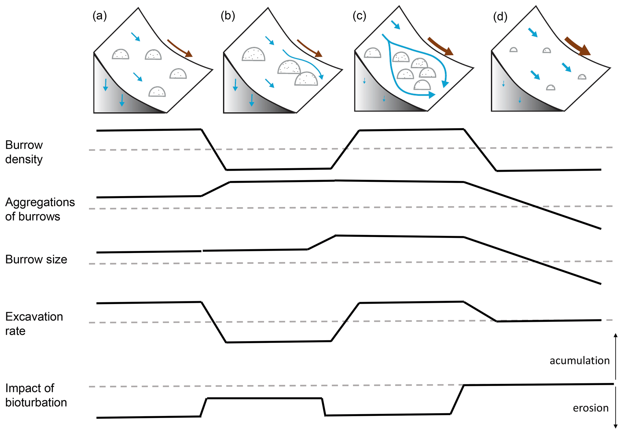
Figure 11 Context dependency of sediment redistribution. (a) Pan de Azúcar, (b) Santa Gracia, (c) La Campana, and (d) Nahuelbuta. Brown arrows indicate the direction and magnitude of overall sediment redistribution within each climate zone. Blue arrows indicate the direction of flow (runoff vs. infiltration). Semicircles indicate the distribution and size of the burrows. The dashed line indicates the median value of each parameter for the first four parameters.

6 Conclusions

Our study found that the inclusion of vertebrate bioturbators' burrows into a soil erosion model significantly increases its reliability. Vertebrate bioturbators increase sediment accumulation in the arid climate zone, increase sediment erosion in the semi-arid and Mediterranean zone, and have no impact on sediment redistribution in the humid zone. Our study furthermore shows that the impact of bioturbation heavily depends on adjacent environmental parameters. The burrows increase sediment erosion at high and low values of elevation; at high values of slope, sink connectivity, and topography ruggedness; and at low values of vegetation cover. The burrows increase accumulation at high values of surface roughness and soil wetness. This means that, overall, on geological timescales, as burrowing animals increase both erosion in steeper zones and accumulation in areas with gentler slopes and higher roughness, hillslope relief should become more quickly equalized and overall more flat. This tendency is most pronounced in the Mediterranean zone with high burrow density and excavation rates, as well as comparably high precipitation rates.

Appendix A

Table A1 R² and RMSE of random forest models trained for the prediction of soil properties needed for model parametrization. RMSE is root mean square error.

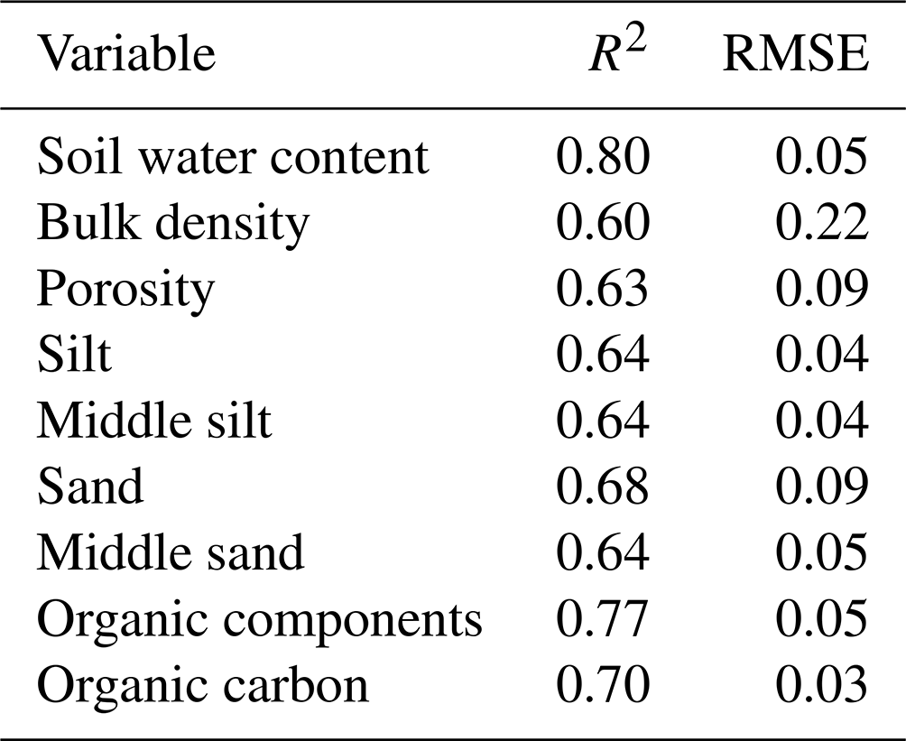
Table A2 Model sensitivity analysis. For the analysis, the minimum, maximum, and mean values of each parameter were calculated. The model was run for a hillslope catchment of 1 km² with homogenous mean parameters. Then, the minimum and maximum values of each parameter were tested. Each parameter was changed stepwise to its minimum or maximum value while the remaining parameters stayed homogenous. The significance of the parameter was estimated by a t test conducted between the erosion estimated by the model with homogenous mean parameters and the erosion estimated by the model with varying minimum and maximum parameter values. Only significant parameters are shown.

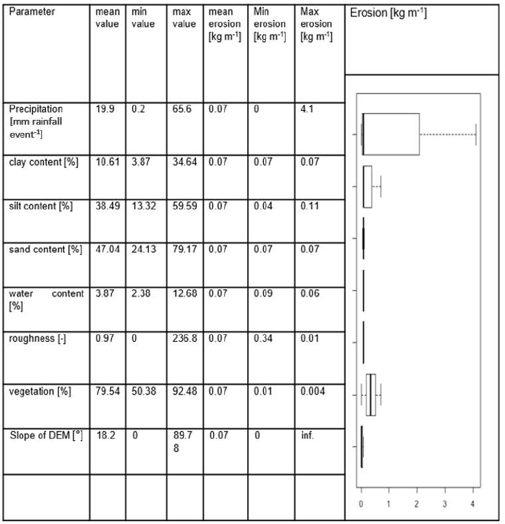
Table A3 Summary of GAM models. We analyzed the impact of parameters within a 1 and 10 m from burrows. The asterisks indicate p values of the selected parameters. ${}^{****}$ p<0.001. ${}^{***}$ p<0.01. ${}^{**}$ p<0.05. ^* p<0.1. One GAM model was run per parameter. Only results for models with an explained variance above 5 % are shown.

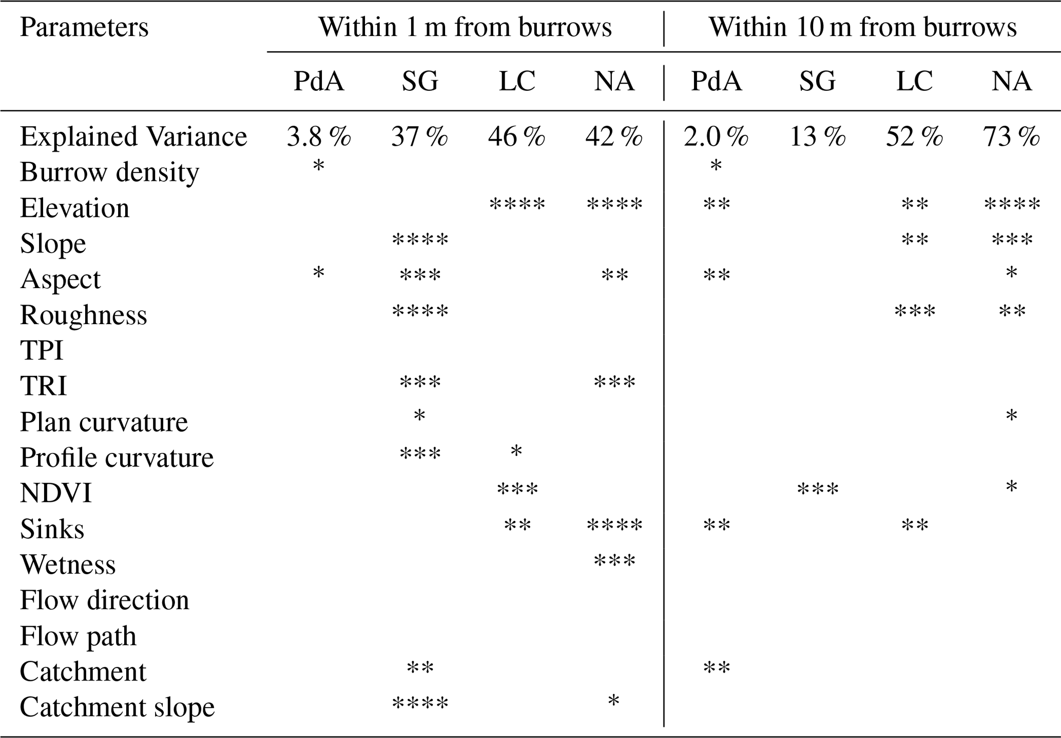
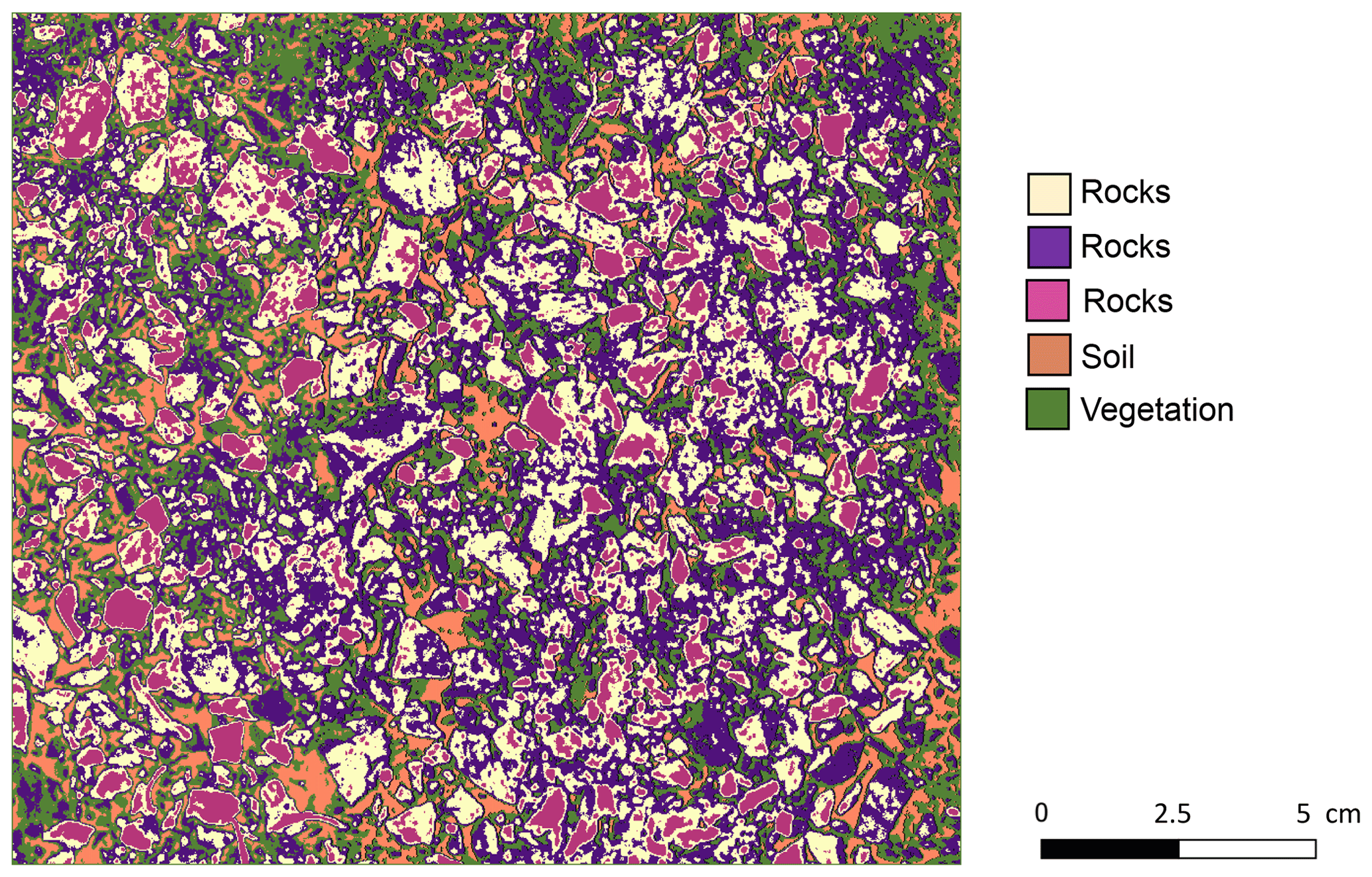
Figure A1 An example of the unsupervised k-means classification of the surface photo from La Campana. Original photo was taken by Paulina Grigusova. The collection of in situ data is explained in Sect. 3.1. and the estimation of soil properties in Sect. 3.2. The image was classified into five classes using unsupervised k-means classification; the land cover was then assigned manually. In some cases, like in this case for rocks, multiple k-means classes stand for the same land cover. These were then unified to the class “rocks”.

Table A4 Review of studies which integrated any kind of bioturbation into models. Previous models integrated either benthic, invertebrate, or single species of vertebrate bioturbators. Models applied described either the vertical soil mixing or long-term landscape evolution models. None of the previous studies included vertebrate burrows of bioturbators into an erosion model which would be capable of capturing the daily redistribution processes.

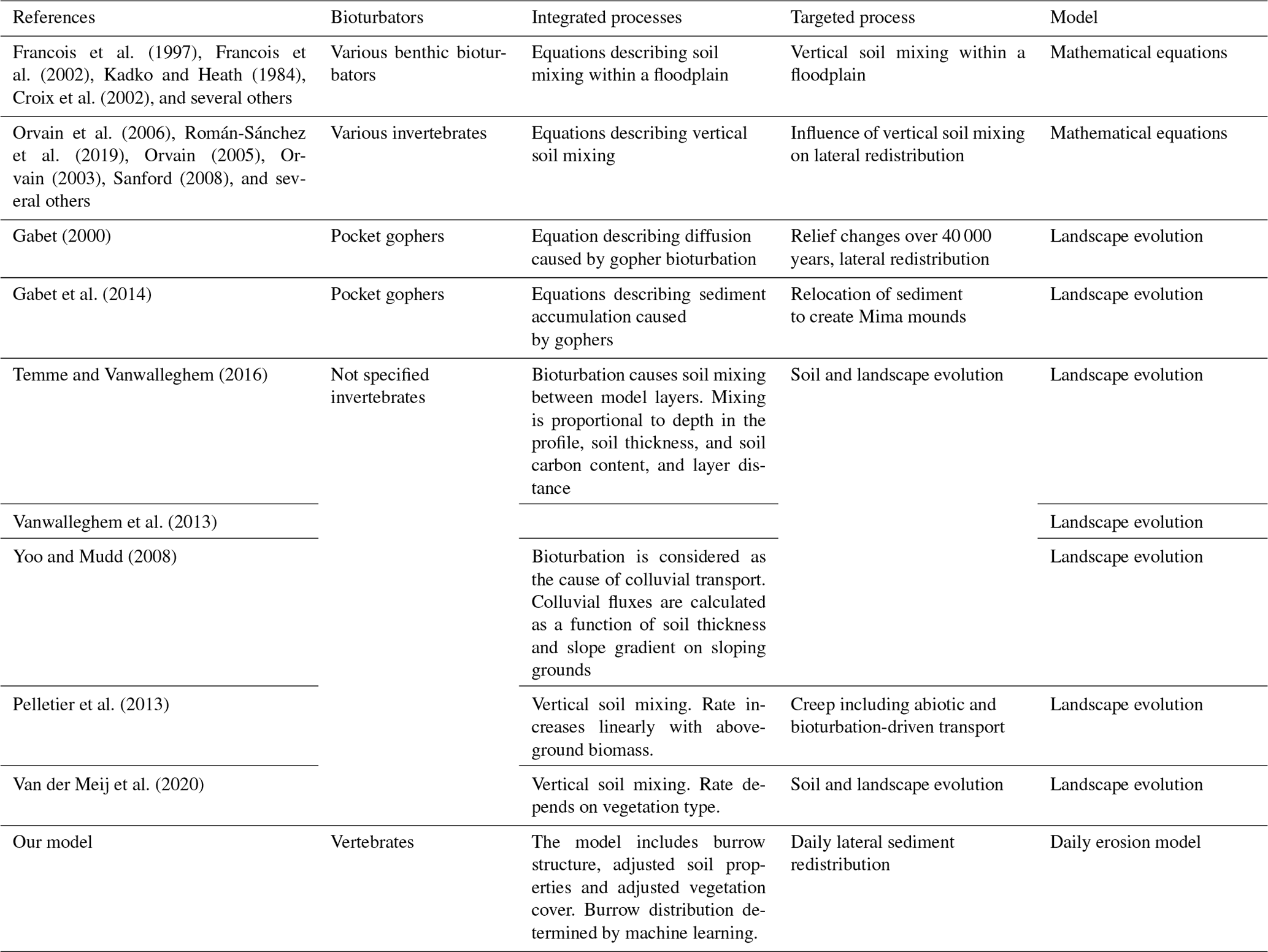
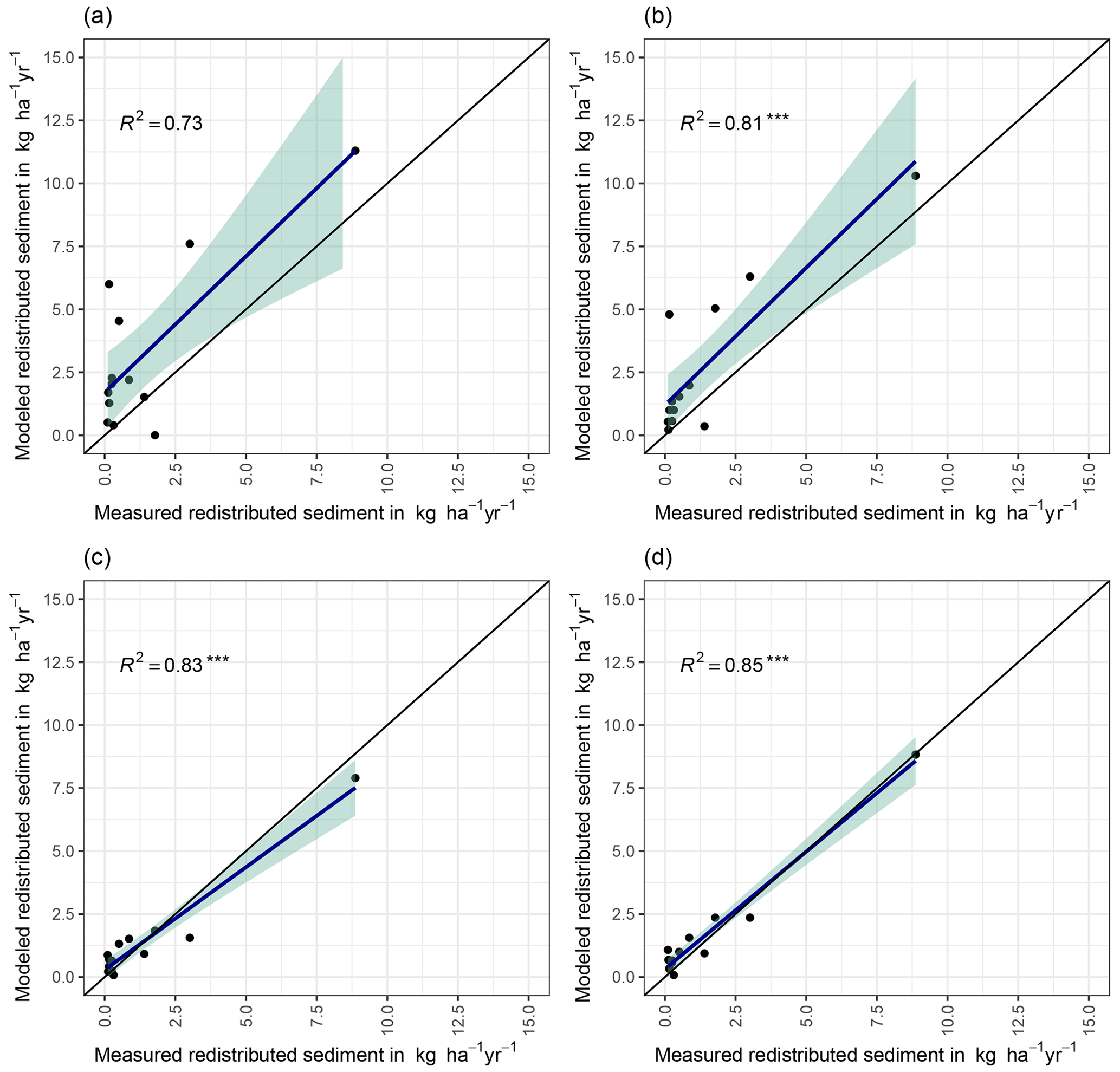
Figure A2 Measured and modeled redistributed sediment for different scenarios. (a) Model without bioturbation. (b) Model with entrances. (c) Model with mounds. (d) Model with burrows.

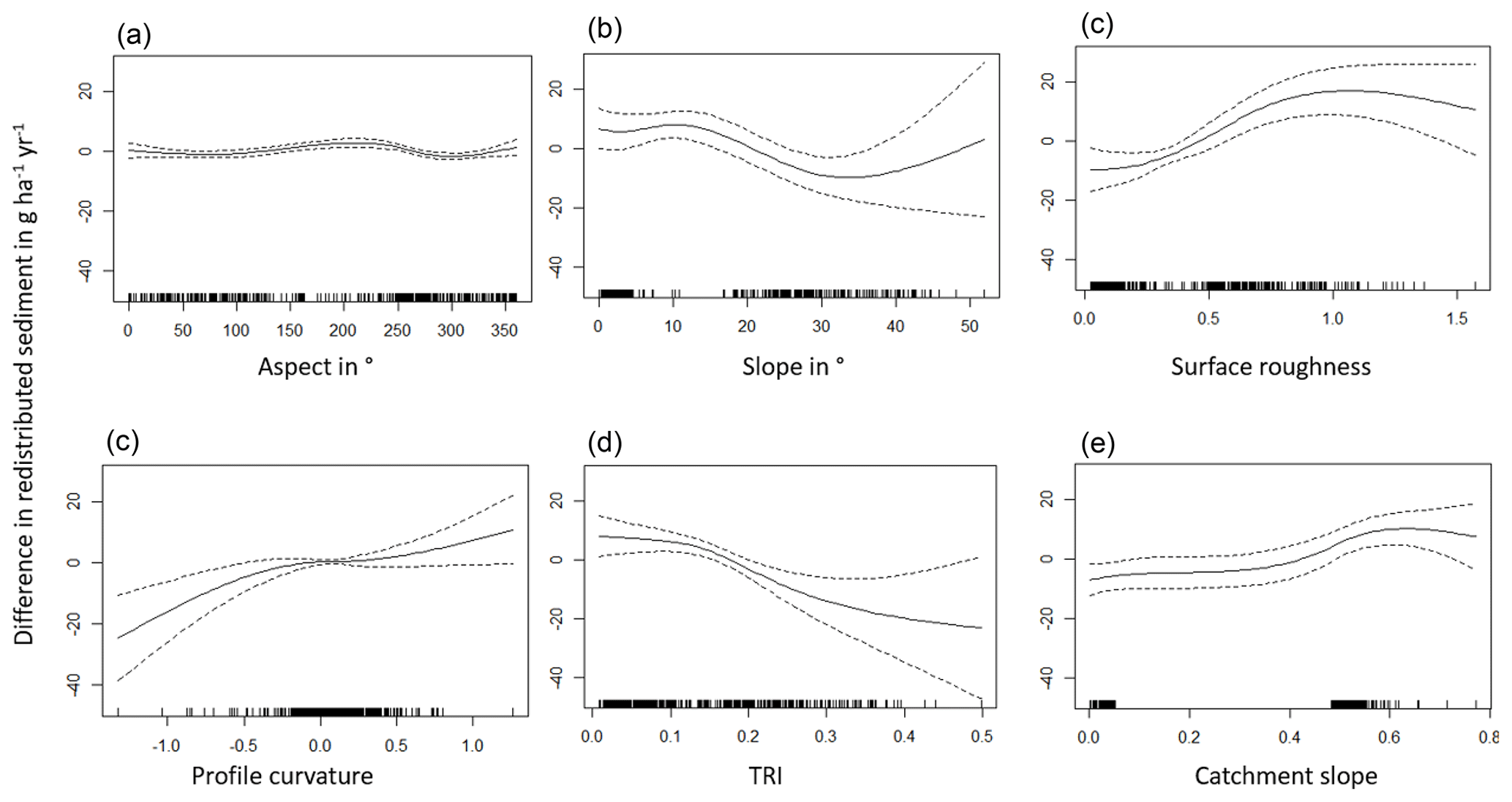
Figure A3 Environmental parameters influencing impact of bioturbation on sediment redistribution in Santa Gracia within 1 m from the burrows. Positive values indicate bioturbation enhances sediment accumulation at the respective parameter values; negative values indicate bioturbation enhances sediment erosion at the respective parameter values.

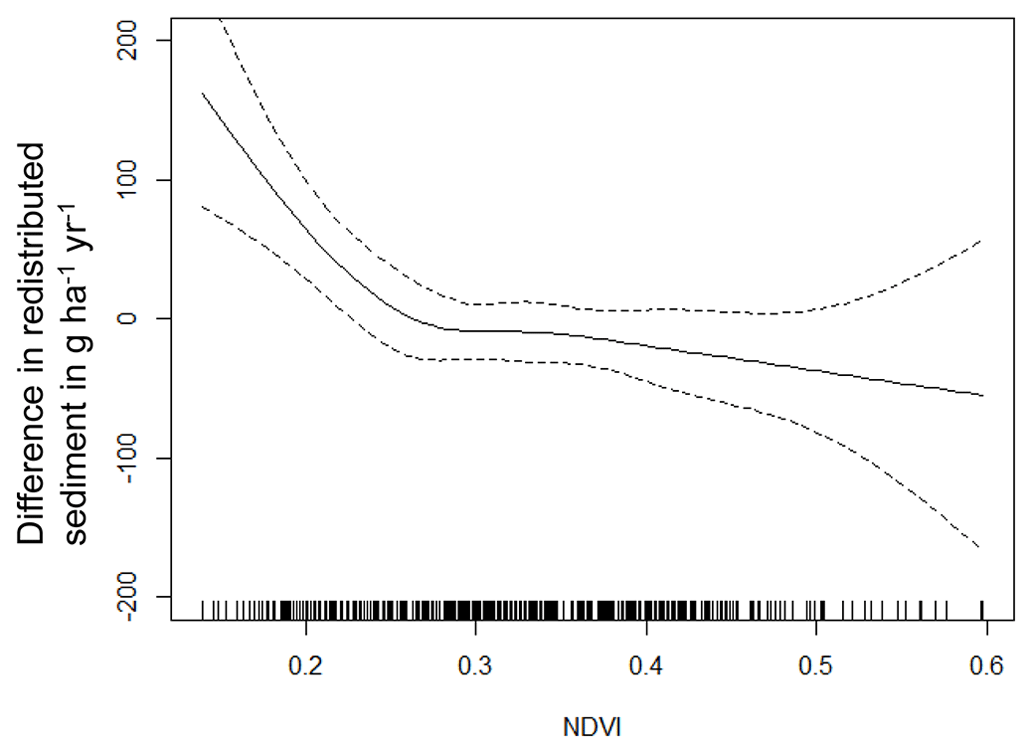
Figure A4 Environmental parameters influencing impact of bioturbation on sediment redistribution in Santa Gracia within 10 m from the burrows. Positive values indicate bioturbation enhances sediment accumulation at the respective parameter values; negative values indicate bioturbation enhances sediment erosion at the respective parameter values.

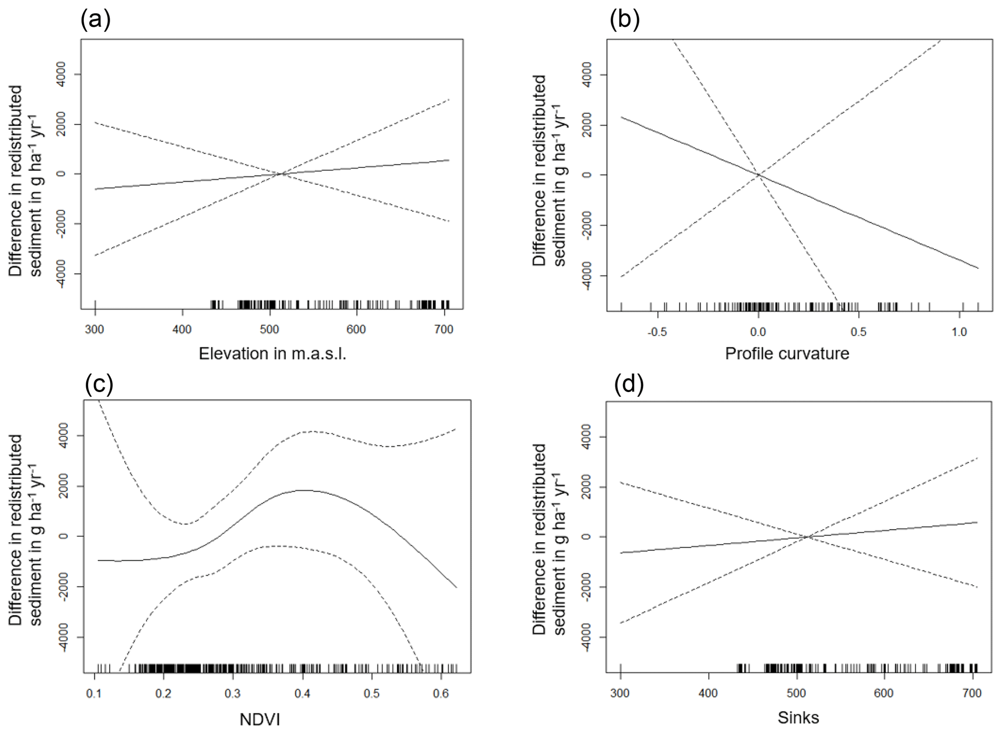
Figure A5 Environmental parameters influencing impact of bioturbation on sediment redistribution in La Campana within 1 m from the burrows. Positive values indicate bioturbation enhances sediment accumulation at the respective parameter values; negative values indicate bioturbation enhances sediment erosion at the respective parameter values.

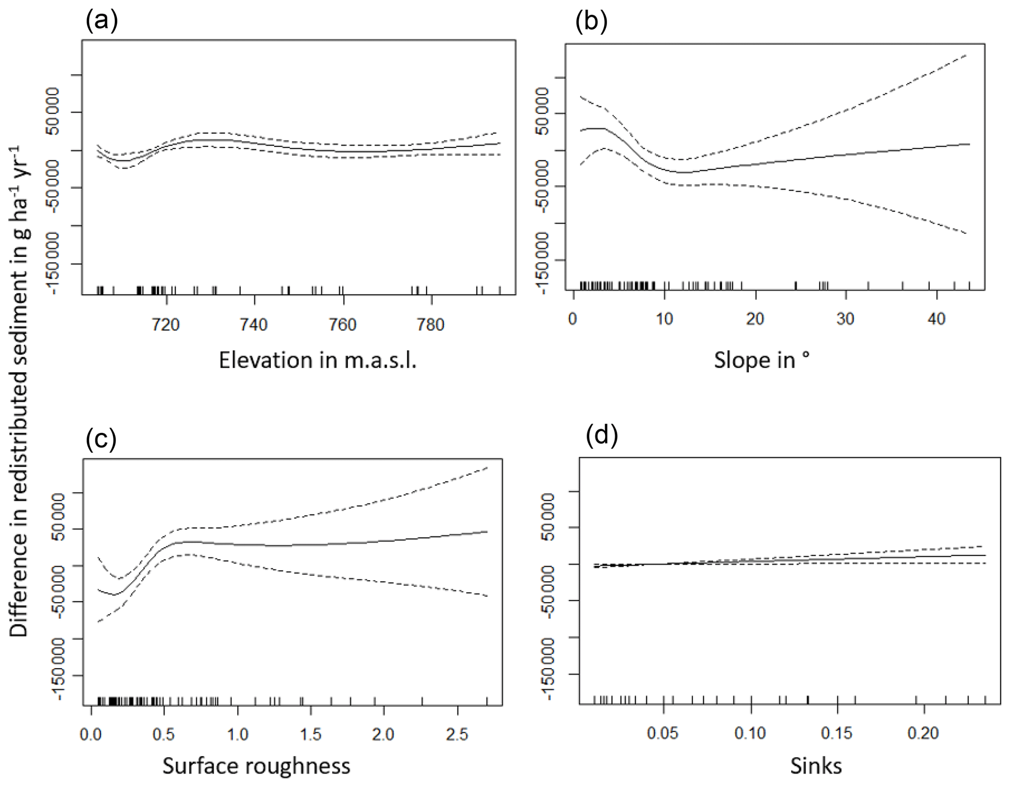
Figure A6 Environmental parameters influencing impact of bioturbation on sediment redistribution in La Campana within 10 m from the burrows. Positive values indicate bioturbation enhances sediment accumulation at the respective parameter values; negative values indicate bioturbation enhances sediment erosion at the respective parameter values.

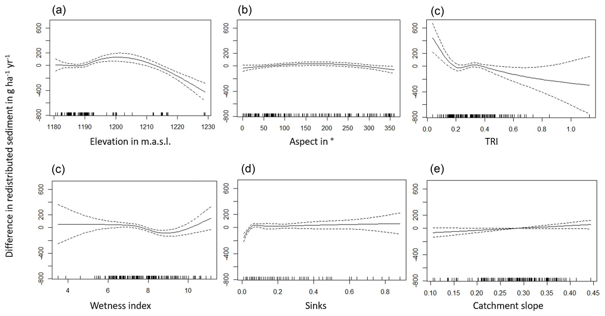
Figure A7 Environmental parameters influencing impact of bioturbation on sediment redistribution in Nahuelbuta within 1 m from the burrows. Positive values indicate bioturbation enhances sediment accumulation at the respective parameter values; negative values indicate bioturbation enhances sediment erosion at the respective parameter values.

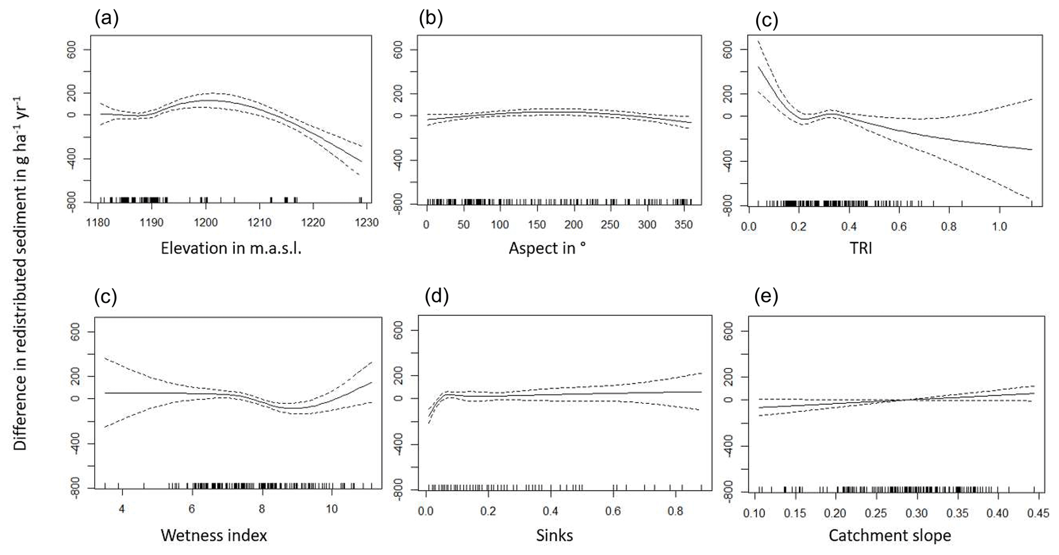
Figure A8 Environmental parameters influencing impact of bioturbation on sediment redistribution in Nahuelbuta within 10 m from the burrows. Positive values indicate bioturbation enhances sediment accumulation at the respective parameter values; negative values indicate bioturbation enhances sediment erosion at the respective parameter values.

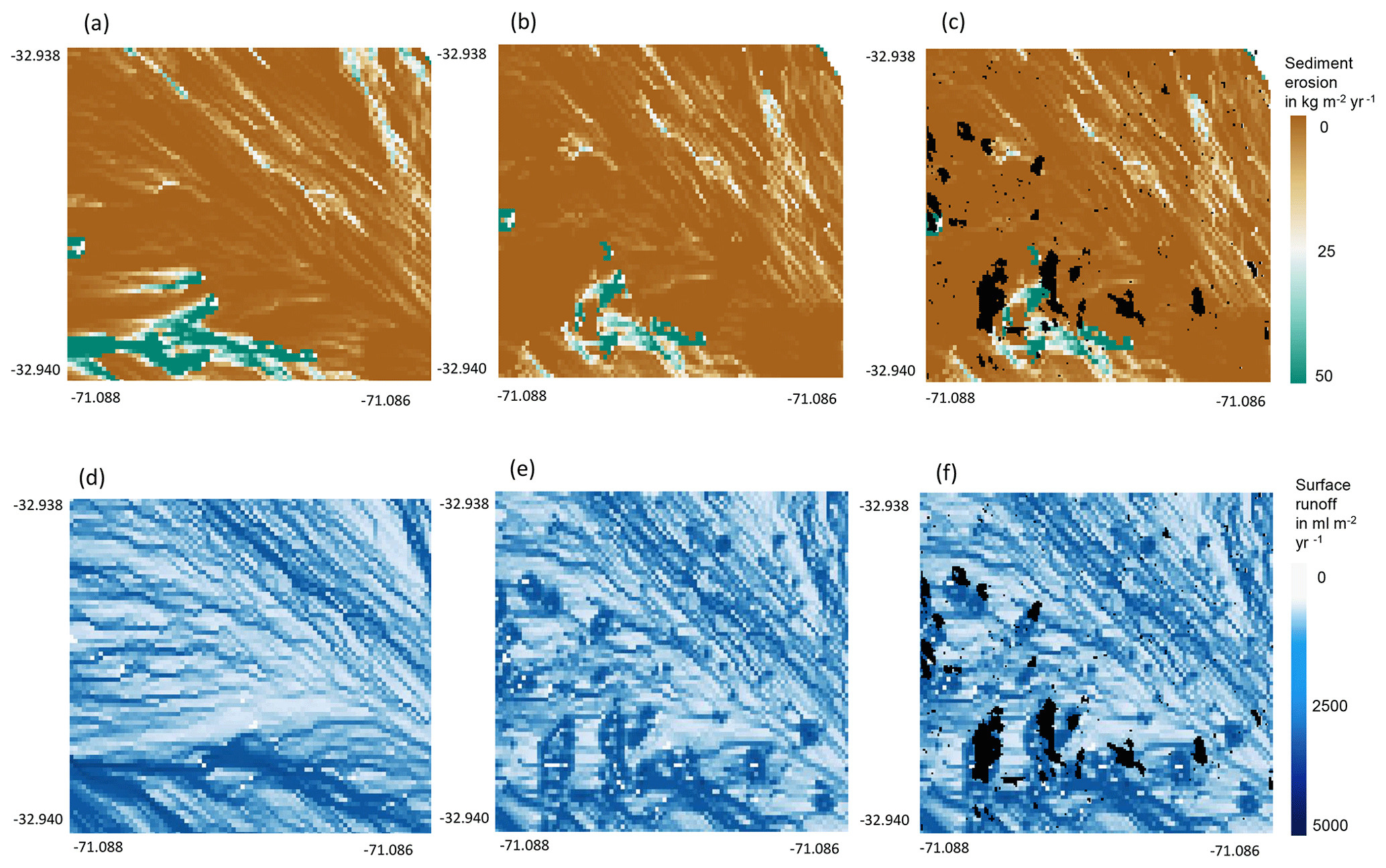
Figure A9 Burrow aggregation concentrates the runoff and increases erosion. An example of a north-facing hillside in Mediterranean La Campana for the time period of 1 year. (a) Sediment erosion as estimated by the model without bioturbation. (b) Sediment erosion as estimated by the model with bioturbation. (c) Sediment erosion as estimated by the model with bioturbation with predicted burrow locations. (d) Surface runoff as estimated by the model without bioturbation. (e) Surface runoff as estimated by the model with bioturbation. (f) Surface runoff as estimated by the model including bioturbation and predicted burrow locations. Black indicates that at least one burrow was located within this pixel. Four neighboring pixels which contain a burrow form a burrow aggregation.

Figure A10 Correlation matrix between the model input parameters.