the Creative Commons Attribution 4.0 License.
the Creative Commons Attribution 4.0 License.
 | 12 Oct 2023
The fingerprint of climate variability on the surface ocean cycling of iron and its isotopes
Alessandro Tagliabue
The essential micronutrient iron (Fe) limits phytoplankton growth when dissolved Fe (dFe) concentrations are too low to meet biological demands. However, many of the processes that remove, supply, or transform Fe are poorly constrained, which limits our ability to predict how ocean productivity responds to ongoing and future changes in climate. In recent years, isotopic signatures (δ56Fe) of Fe have increasingly been used to gain insight into the ocean Fe cycle, as distinct δ56Fe endmembers of external Fe sources and δ56Fe fractionation during processes such as Fe uptake by phytoplankton can leave a characteristic imprint on dFe signatures (δ56Fediss). However, given the relative novelty of these measurements, the temporal scale of δ56Fediss observations is limited. Thus, it is unclear how the changes in ocean physics and biogeochemistry associated with ongoing or future climate change will affect δ56Fediss on interannual to decadal timescales. To explore the response of δ56Fediss to such climate variability, we conducted a suite of experiments with a global ocean model with active δ56Fe cycling under two climate scenarios. The first scenario is based on an atmospheric reanalysis and includes recent climate variability (1958–2021), whereas the second comes from a historical and high-emissions climate change simulation to 2100. We find that under recent climatic conditions (1975–2021), interannual δ56Fediss variability is highest in the tropical Pacific due to circulation and productivity changes related to the El Niño–Southern Oscillation (ENSO), which alter both endmember and uptake fractionation effects on δ56Fediss by redistributing dFe from different external sources and shifting nutrient limitation patterns. While the tropical Pacific will remain a hotspot of δ56Fediss variability in the future, the most substantial end-of-century δ56Fediss changes will occur in the Southern Hemisphere at middle to high latitudes. These arise from uptake fractionation effects due to shifts in nutrient limitation. Based on these strong responses to climate variability, ongoing measurements of δ56Fediss may help diagnose changes in external Fe supply and ocean nutrient limitation.
- Article
(7896 KB) - Full-text XML
-
Supplement
(4151 KB) - BibTeX
- EndNote


The micronutrient iron (Fe) is thought to control primary productivity in large parts of the global ocean where limited supply and/or rapid removal keep dissolved Fe (dFe) concentrations low. However, our understanding of the ocean Fe cycle is still limited, as it involves a multitude of internal cycling processes and various supply mechanisms, both of which are often poorly constrained (Boyd and Ellwood, 2010; Tagliabue et al., 2017). One way to help disentangle the web of processes and sources is to measure the isotopic signatures of Fe (namely ), as some Fe cycle processes distinctively alter δ56Fe via fractionation and many external sources of Fe have characteristic δ56Fe endmember signatures. Thus, δ56Fe has been used to study various aspects of the ocean cycle. For instance, changes in δ56Fe of the dissolved and particulate Fe pools have been observed for different phytoplankton bloom stages, indicating that phytoplankton may preferentially take up light Fe so that the δ56Fe of the dFe pool (δ56Fediss) becomes increasingly heavy (Ellwood et al., 2015). Consequently, heavy δ56Fediss observed in other low dFe surface ocean systems were suggested to be due to ongoing phytoplankton uptake and biological recycling, possibly combined with fractionation during the complexation of Fe by organic ligands (Ellwood et al., 2020; Sieber et al., 2021). On the other hand, the distinct δ56Fe endmembers of external sources have been used in mass balance approaches (of δ56Fediss and dFe) to estimate the relative importance of each source in supplying new Fe (Conway and John, 2014; Pinedo-González et al., 2020). Such approaches take advantage of the wide range of source δ56Fe endmembers from exceedingly light δ56Fe associated with reductive sediments (as low as −3.3‰; Homoky et al., 2009; Severmann et al., 2010) and aeolian Fe from anthropogenic emissions (as low as −4.0 ‰, Kurisu et al., 2019) to crustal δ56Fe (ca. 0.1 ‰) for dFe supplied by non-reductive sedimentary processes or dust deposition (Conway et al., 2019; Homoky et al., 2013; Radic et al., 2011; Waeles et al., 2007).
Overall, δ56Fediss is likely determined by a combination of δ56Fe fractionation during internal cycling and supply of new Fe from external sources with characteristic δ56Fe endmembers (König et al., 2021, 2022). Both variable source endmembers and fractionation during phytoplankton uptake and organic complexation are needed for a global Fe isotope model to reasonably reproduce δ56Fediss observations (König et al., 2021). However, most δ56Fediss observations and the majority of dFe concentration measurements have been obtained from single occupations of stations as part of GEOTRACES transects and from a few process studies, one of which focuses on seasonal changes (Ellwood et al., 2015). Consequently, there is only limited observation-based information available about the temporal variability in δ56Fediss (and Fe cycling in general) and its response to changes in ocean physics driven by climate variability. So far, only one study has reported repeat δ56Fediss measurements from re-occupations of three different stations in the Atlantic (Conway et al., 2016). While at each station the shape of the δ56Fediss profiles in this work was similar for both occupations, some discrepancies were detected for the station near Cabo Verde and the upper part of the profile in Cape Basin near South Africa. Variable δ56Fediss near Cabo Verde were suggested to be related to changes in the relative contribution of dFe from different external sources, namely Fe supply by reductive sediments and dust dissolution. In the Cape Basin, changes in surface currents were thought to be responsible, as the differences in upper ocean δ56Fediss and dFe coincided with changes in temperature, oxygen, and salinity. These observations suggest that δ56Fediss can vary over interannual timescales, especially in the upper ocean. Substantial temporal variability in local Fe sources and cycling has also been observed for repeat measurements of Fe concentration at time series stations in the North Pacific, Atlantic, and Mediterranean (Bonnet and Guieu, 2006; Fitzsimmons et al., 2015; Nishioka et al., 2001; Schallenberg et al., 2015; Sedwick et al., 2005, 2020), but no parallel Fe isotope measurements were made.
Modelling work suggests that seasonal variability in dFe supply from aeolian deposition and winter mixing can induce variability in surface ocean δ56Fediss both directly and indirectly (König et al., 2022). Direct effects occur due to the variable δ56Fe endmembers of each source, and indirect effects also arise as differences in Fe supply can change the degree of δ56Fe fractionation during phytoplankton uptake and/or complexation by organic ligands. The change in the degree of uptake fractionation is suggested to be greatest in areas where Fe was the limiting nutrient of primary production. However, while aeolian Fe deposition varied among the years in this study, changes in ocean physics driven by climate variability were not accounted for, as the same (seasonally variable) physical forcing fields were applied each year. We would expect climate-driven changes in ocean circulation to induce similar, if not larger, changes in δ56Fediss than variable external Fe supply, as such changes can redistribute dFe and other nutrients more significantly. Changes in nutrient availability and other parameters (e.g. temperature) can then lead to shifts in local upper ocean biogeochemistry, potentially altering the effect of fractionating processes on δ56Fediss, for instance during phytoplankton uptake (Ellwood et al., 2015). On interannual timescales, climate-related changes in ocean physics are mainly driven by climate variations such as the Southern Annular Mode or the El Niño–Southern Oscillation (ENSO), which has been shown to impact Fe cycling in the California Current System (Johnson et al., 1999). On longer timescales, global warming will likely lead to changes in ocean physics and, consequently, biogeochemistry, where the extent of such effects depends on current and future CO2 emissions (Bindoff et al., 2019; Kwiatkowski et al., 2020), but their effects on Fe and Fe isotopes remain poorly constrained.
To test how surface ocean δ56Fediss responds to interannual and decadal climate variability, we set up two sets of model experiments. In a set of hindcast simulations, variability in ocean physics was driven by the inherent variability in an atmospheric reanalysis product, covering the years 1958 to 2021. In a second set of experiments, we used outputs from a 249-year climate change simulation (1852–2100), which includes internal climate variability as well as effects of long-term global warming. These experiments allowed us to detect hotspots of surface ocean δ56Fediss variability in the present and future climate and identify the driving forces behind such variability.
2.1 Experimental design
We conducted both sets of experiments (referred to as “hindcast” and “climate change”) by applying offline physical forcing fields to a version of the PISCES biogeochemical ocean model with active δ56Fe cycling, which has been used previously to study the effect of internal cycling and (variable) external δ56Fe endmembers on δ56Fediss (König et al., 2021, 2022). This model is based on PISCES-v2 (Aumont et al., 2015) which represents two phytoplankton, two zooplankton, and two particle size classes (with variable particle reactivity; Aumont et al., 2017), five nutrients (NO3, NH4, PO4, Fe, and Si), oxygen, and the carbonate system. Its Fe cycle representation is comparably complex (Tagliabue et al., 2016), and includes a prognostic Fe-binding ligand tracer (Völker and Tagliabue, 2015) and Fe input from four external sources (rivers, hydrothermal vents, dust deposition, sediments) plus sea ice (source or sink; Aumont et al., 2015). In the δ56Fe version of this model, each Fe tracer is split into a heavy (56Fe) and light (54Fe) pool (König et al., 2021), as illustrated for heavy and light dFe in Text S1 in the Supplement. Distinct δ56Fe endmembers are applied to each of the four external Fe sources and δ56Fe fractionation is applied to two of the internal cycling processes: complexation by organic ligands (preference for heavy 56Fe) and uptake by phytoplankton (preference for light 54Fe; König et al., 2021; Text S1).
For the hindcast model experiments, we applied 5 d physical forcing fields obtained from coupled NEMO-SI3–PISCES simulations forced by the JRA-55 atmospheric reanalysis (Tsujino et al., 2018), as described in Buchanan and Tagliabue (2021), extended to 2021. We conducted three repeat cycles of the 64-year period (1830–2021). As changes in climate in the later years of the cycle may impact the earlier years of the last repeat cycle, we focus on the last 46 years of each simulation (1975–2021).
To investigate the impact of climate change on δ56Fediss, we set up climate change simulations using offline forcing fields from the IPSL-CM5A climate model (Dufresne et al., 2013), as described in previous studies (e.g. Richon and Tagliabue, 2021). For each experiment (i.e. standard simulation and sensitivity tests), we first set up pre-industrial (PI) control simulations from 1801 to 2100 using forcings from an IPSL-CM5A experiment with fixed pre-industrial atmospheric CO2. We then set up climate change experiments from 1852 to 2100, initialized using the 1851 PI control output and forced by fields from IPSL-CM5A experiments with atmospheric CO2 concentrations following historical pathways until 2005 and switching to the high-emissions RCP8.5 scenario thereafter.
2.2 Sensitivity experiments and isolating δ56Fediss components
We conducted an equivalent set of “standard” δ56Fe model simulations and sensitivity tests for both hindcast and climate change physical settings (Table 1). For the standard simulations, we used the δ56Fe model set-up described in König et al. (2021), whereas for the sensitivity experiments we turned off either uptake or complexation fractionation by setting their respective fractionation factors to 1. This allowed us to estimate the extent of δ56Fediss variability that is caused by changes in fractionation and source endmember effects, using the following set of calculations.
Firstly, we “split up” δ56Fediss into uptake fractionation (δ56FeUF), complexation fractionation (δ56FeCF), and endmember (δ56FeEM) contributions, i.e. the effect which each fractionation process and the source endmembers have on “overall” δ56Fediss. In the case of δ56FeUF and δ56FeCF, we calculated their respective contributions using the δ56Fediss of the standard experiment and those obtained from sensitivity experiments where either the uptake fractionation factor (“noUF”) or complexation fractionation factor (“noCF”) was set to 1 (Eqs. 1 and 2).
Thanks to the additive nature of fractionation and endmember effects in our model, which we confirmed for the hindcast experiments (Fig. S1 in the Supplement), the endmember effect δ56FeEM could be calculated by subtracting the two fractionation effects from δ56Fediss (Eq. 3).
We also set up an experiment (“neuSED”) where the sediment δ56Fe endmember was set to 0 ‰ (only for the hindcast physical setting) to study endmember effects in areas where the surface ocean sediment endmember of the model (−1 ‰; König et al., 2021) is likely too light (Sect. 4.1).
2.3 Determining interannual variability in δ56Fediss and its components
To quantify the interannual variability in δ56Fediss and its three components (δ56FeUF, δ56FeUF, and δ56Fe), we first applied a 12-month running mean boxcar filter to each value (which were based on monthly model output) to smooth out seasonal effects. We then calculated the interannual variance (VAR) and standard deviation (SD) for δ56Fediss and for each component over the respective time periods of interest (1975–2021 for the hindcast and 2006–2100 for the climate change experiments). Note that we focus here on the surface ocean (0–10 m), as δ56Fediss variability beneath the surface is often driven by small lateral or vertical movement in steep δ56Fediss gradients, for instance, due to shifts in mixed layer depth. To compare the interannual variability in each of the three components to δ56Fediss variability, we calculated the “relative variability”, i.e. the ratio of their VAR to that of δ56Fediss, where subscript i = UF, CF, or EM (Eq. 4).
Note that the sum of the three ratios is less (greater) than 1 in areas with positive (negative) covariance between two or three of the components, i.e. where their responses to climate variability are reinforcing (opposing) each other.
3.1 Hotspots of present and future δ56Fediss variability in the surface ocean
3.1.1 Areas of high δ56Fediss variability in the present climate (1975–2021)
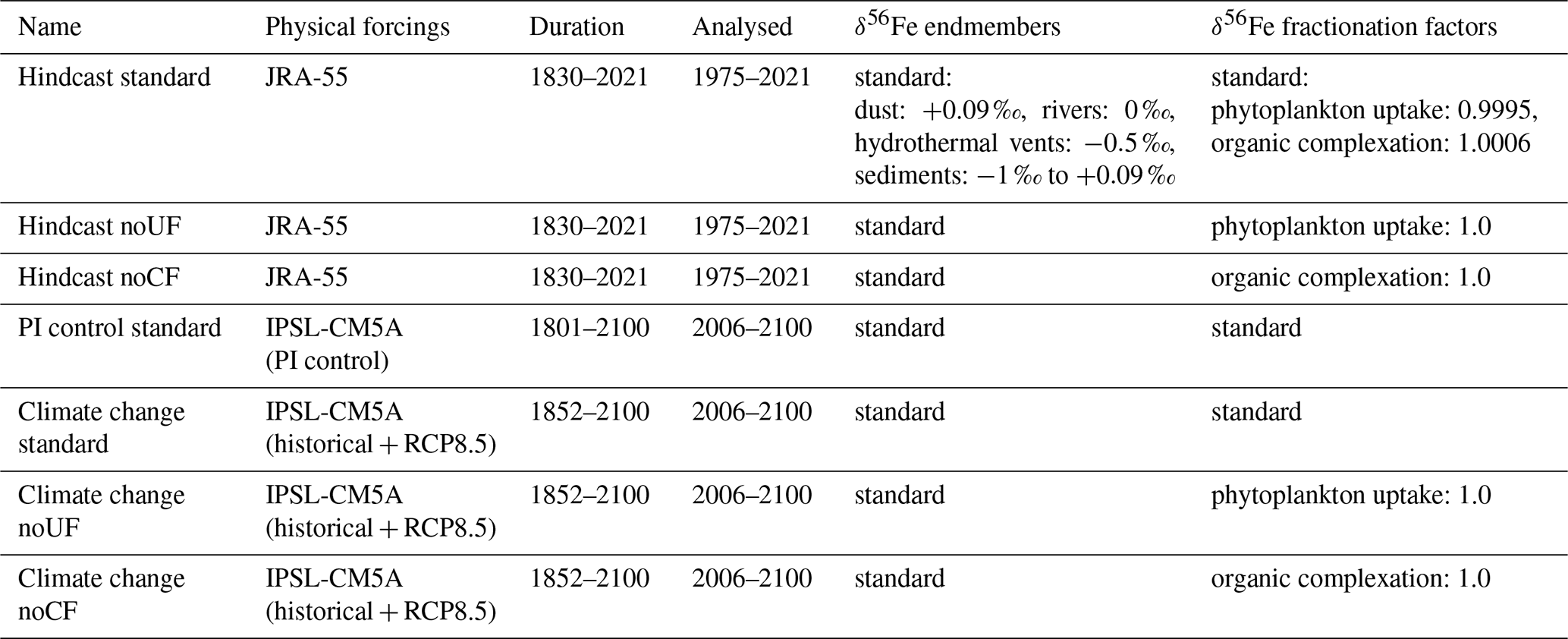
In the 1975–2021 period of the hindcast simulations, interannual surface ocean δ56Fediss variability is highest in the tropical Pacific due to multiple drivers. This is illustrated by maxima in the interannual δ56Fediss SD, with additional areas of localized elevated variability present around 40∘ S (Fig. 1a). Interestingly, there appears to be no obvious connection between the interannual δ56Fediss SD and the interannual SD of dFe concentration and primary productivity (Fig. S2), indicating that (absolute) changes in these values are not (solely) driving δ56Fediss variability. Comparing this δ56Fediss SD to the average δ56Fediss values (Fig. 1b) indicates that the δ56Fediss SD is often elevated in areas with steep horizontal δ56Fediss gradients, with shifts in circulation causing local changes in δ56Fediss. Elevated variability in δ56FeUF and δ56FeEM (Fig. 1c, d) suggests that the high δ56Fediss variability in the tropical Pacific during our simulations is due to changes in both uptake fractionation and the circulation of external source δ56Fe endmembers. At high latitudes, a combination of changes in uptake and, to a lesser extent, complexation fractionation appear to drive δ56Fediss variability (Fig. 1c, e), although variability is generally lower in these areas (Fig. 1a). The elevated δ56Fediss SD at around 40∘ S is caused by horizontal shifts in areas with heavy δ56Fediss likely related to strong (accumulated) uptake fractionation effects (Fig. 1c), as discussed in Sect. 4.2. Note that covariance between the components can be substantial for some regions, especially between δ56FeUF and δ56FeEM (Fig. 1f), which can increase or decrease the δ56Fediss variability, depending on location (Fig. S3). Furthermore, δ56Fediss variability (unsurprisingly) increases when seasonal effects are accounted for (by calculating δ56Fediss SD from monthly model outputs without applying a 12-month running mean; Fig. S4). Seasonal effects are thereby largest at high latitudes mostly due to uptake fractionation effects, especially in the Southern Hemisphere (south of ca. 40∘ S). However, a combination of endmember changes due to ocean circulation and uptake fractionation remain important in the tropical Pacific (Fig. S4).
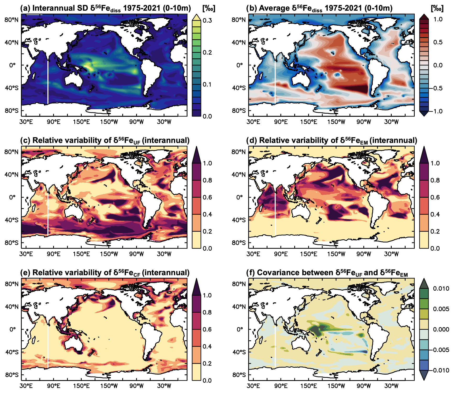
Figure 1Surface ocean δ56Fediss interannual variability and its drivers in the present climate (1975–2021). Surface ocean (0–10 m) (a) interannual δ56Fediss SD (‰) and (b) average δ56Fediss (‰) of the hindcast standard experiment. Ratios of interannual variability in (c) δ56FeUF, (d) δ56FeEM, and (e) δ56FeCF to interannual δ56Fediss variability (Eq. 4); drivers are denoted as “endmembers” (EM), “uptake fractionation” (UF), “complexation fractionation” (CF), and various combinations thereafter. (f) Covariance between δ56FeUF and δ56FeEM (12-month running mean).
3.1.2 Future δ56Fediss variability (2006–2100) due to climate change
The major changes in ocean circulation and physical conditions in our high-emissions climate change experiments lead to substantial δ56Fediss variability over the next century. The interannual δ56Fediss SD over the 2006–2100 period of our climate change simulation is considerably higher than for the parallel PI control simulation without any climate change effects (and higher than for the hindcast simulation, Fig. 2a and b). Over the shorter period of the hindcast experiments (1975–2021), elevated δ56Fediss SD is mainly due to temporal variability around a mean δ56Fediss value, whereas for the climate change experiments, elevated δ56Fediss SD is also related to a change in the mean δ56Fediss over the next century (Sect. 3.3). The δ56Fediss SD of the PI control thereby resembles that of the standard hindcast experiment (Fig. 1a; note difference in scale), with some discrepancies due to the differences in model circulation.
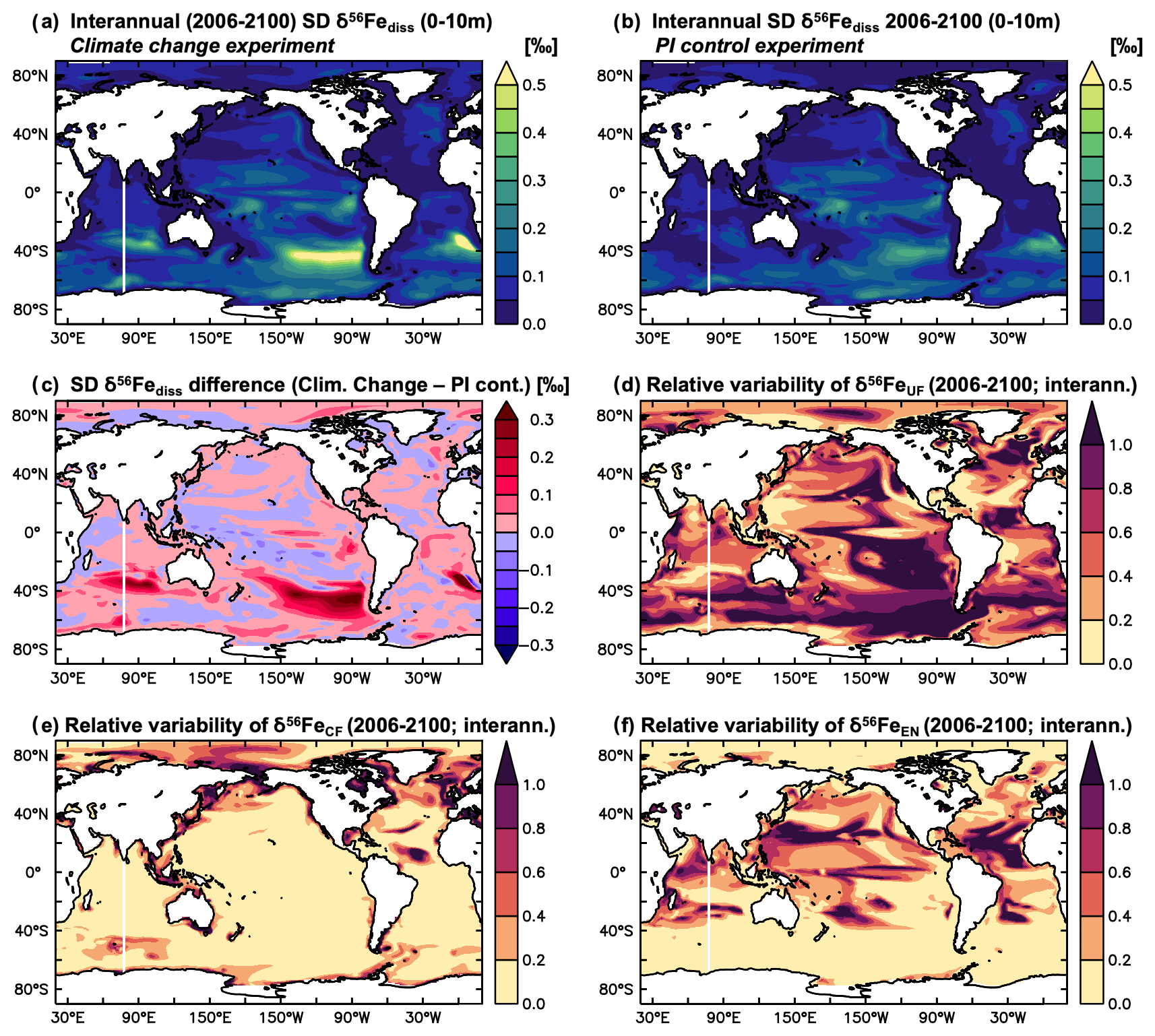
Figure 2Surface ocean δ56Fediss interannual variability under future climate scenarios (2006–2100). Surface ocean (0–10 m) interannual SD δ56Fediss (‰) for (a) climate change and (b) PI control experiments, and (c) the difference between the two (i.e. climate change SD δ56Fediss − PI control SD δ56Fediss; ‰). Ratios of interannual variability in (d) δ56FeUF, (e) δ56FeCF, and (f) δ56FeEM to interannual δ56Fediss variability (Eq. 4).
In the tropical Pacific, where interannual δ56Fediss SD was highest over the period covered by the hindcast experiment (1975–2021; Fig. 1a), variability remains high under future climate change conditions (Fig. 2a). However, while the magnitude of δ56Fediss SD is similar for the climate change experiment, there are some regional differences. δ56Fediss SD is elevated in the eastern equatorial Pacific compared to the PI control but lower in the western part and subtropical regions (Fig. 2c). Generally, a combination of both endmember (δ56FeEM) and uptake fractionation (δ56FeUF) effects appears to be responsible for the δ56Fediss variability in the tropical Pacific (Fig. 2d, f), similar to the hindcast experiment (Fig. 1f); however, in the eastern equatorial Pacific where δ56Fediss variability increased, δ56FeEM appears to be the controlling factor (see also Sect. 3.2.3).
A notable increase in interannual δ56Fediss variability due to climate change occurs in the Southern Hemisphere. In the region between ca. 30 and 50∘ S (Fig. 2a, b), where δ56Fediss SD was already elevated under present climate conditions (hindcast simulation; Fig. 1a), δ56Fediss SD more than doubles due to climate change (Fig. 2c). While some of this variability seems to be related to endmember effects (δ56FeEM), changes in uptake fractionation (δ56FeUF) appear to dominate the future δ56Fediss variability in most of the Southern Hemisphere at middle to high latitudes (Fig. 2d). This is due to changes in δ56FeUF between 2006 and 2100 caused by the impact of climate change on primary production (Sect. 3.3).
3.2 δ56Fediss variability in the tropical Pacific
3.2.1 Current (1975–2021) δ56Fediss variability in the tropical Pacific driven by ENSO variability
In the tropical Pacific, where δ56Fediss variability in the hindcast simulation is highest (Fig. 1), there is a clear link between surface ocean δ56Fediss and changes in sea surface temperature (SST) associated with different ENSO phases. This can be illustrated by focussing on the equatorial region between 5∘ S and 5∘ N (Fig. 3). As the hindcast simulations were forced by an atmospheric reanalysis product (see Sect. 2), the modelled changes in SST agree very well with observations in the equatorial Pacific, including the timing and extent of the El Niño and La Niña transitions (Fig. S5).
Figure 3Variability in SST as well as δ56Fediss and its drivers in the equatorial Pacific from the hindcast experiment. Time series (1975–2021) of monthly mean surface ocean (a) SST anomaly (∘C) and Ocean Niño Index (ONI; red: El Niño, grey: La Niña), (b) SST (∘C), (c) δ56Fediss (‰), (d) δ56FeEM (‰), and (e) δ56FeUF (‰), averaged from 5∘ N to 5∘ S. The SST anomaly was calculated by subtracting the 1975–2021 average SST from the monthly outputs. The Ocean Niño Index uses the same key as the SST anomaly and was calculated from smoothed SST anomalies (3-month running mean) of the ENSO 3.4 region (120–170∘ W, 5∘ N–5∘ S).
In neutral or weak El Niño/La Niña phases, when SST anomalies and Ocean Niño Index (ONI) are less than ca. ± 0.5 ∘C (Fig. 3a), δ56Fediss is light ( ‰) close to the continental margins of Papua New Guinea (PNG) in the west and South America in the east and heavier in the offshore regions of the open ocean (up to >1 ‰; Fig. 3c). However, during an El Niño event, the area of light surface ocean δ56Fediss close to the PNG margin expands eastward (Fig. 3c), with similar timing and extent as the characteristic warming signal observed in the central and eastern equatorial Pacific (Fig. 3a, b). While these changes are visible in all El Niño years, they are most prominent for the very strong El Niño events of 1982/1983, 1997/1998, and 2015/2016. During these three extreme events (dark red ONI), surface ocean δ56Fediss becomes anomalously light in most areas along the Equator, except in the easternmost part (around 120∘ W), where it is heavier (Fig. 3c). For weaker El Niños (light red ONI) and those where the maximum SST anomalies occur in the centre of the equatorial Pacific, the light δ56Fediss anomaly is restricted to the western part of the equatorial Pacific (Fig. 3c). Conversely, La Niñas events (grey ONI) are associated with a δ56Fediss decrease in the eastern part of the basin, albeit to a lesser degree than for strong El Niños, as the light δ56Fediss area close to the South American margin expands westward (Fig. 3c).
3.2.2 Mechanisms behind ENSO-driven δ56Fediss variability
Splitting δ56Fediss into its main drivers in the tropical Pacific, δ56FeEM and δ56FeUF, shows that δ56Fediss variability during ENSO cycles is due to a combination of endmember and uptake fractionation effects (Fig. 3d, e). These δ56FeEM and δ56FeUF changes are due to circulation changes which affect the redistribution of Fe from external sources and lead to changes in primary productivity and, consequently, Fe uptake rates. We illustrate this with a schematic of the main mechanisms involved (Fig. 4), and use the time period 1995–1996 as an example, as it includes a very strong El Niño followed by a strong La Niña (Fig. 5). During El Niño events, such as in 1997, the weakened trade winds lead to a reversal in the upper ocean currents from predominantly westward flow to eastward flow in most equatorial regions (Figs. 4a, b; 5h). This reversal has far-reaching effects on upper ocean biogeochemistry and Fe cycling, such as higher dFe concentrations in the west, lower concentrations in the east (Fig. 5d), and a general decrease in the ratio of Fe uptake to dFe concentration (Fig. 5e), Fe limitation (Fig. 5f), and primary productivity (Fig. 5g). These changes, in turn, impact δ56FeEM (Fig. 5b) and δ56FeUF (Fig. 5c), as discussed below. Eventually, as the El Niño event breaks down, the incoming La Niña leads to westward currents across the basin (Fig. 4c), which are even stronger than in the neutral phase that precedes El Niño (Fig. 4a), as exemplified by the transition in 1998 (Fig. 5). Note that the same mechanisms also operate during El Niños or La Niñas that are weaker than those of 1997/1998 but to a lesser extent, leading to reduced changes in the parameters in question (Fig. S6). Furthermore, similarly decreasing trends in dFe concentration and primary productivity as simulated by our model for the equatorial Pacific (Fig. 5) have also been observed in the California Current System during the 1997/1998 El Niño, where coastal upwelling was also suppressed (Johnson et al., 1999).
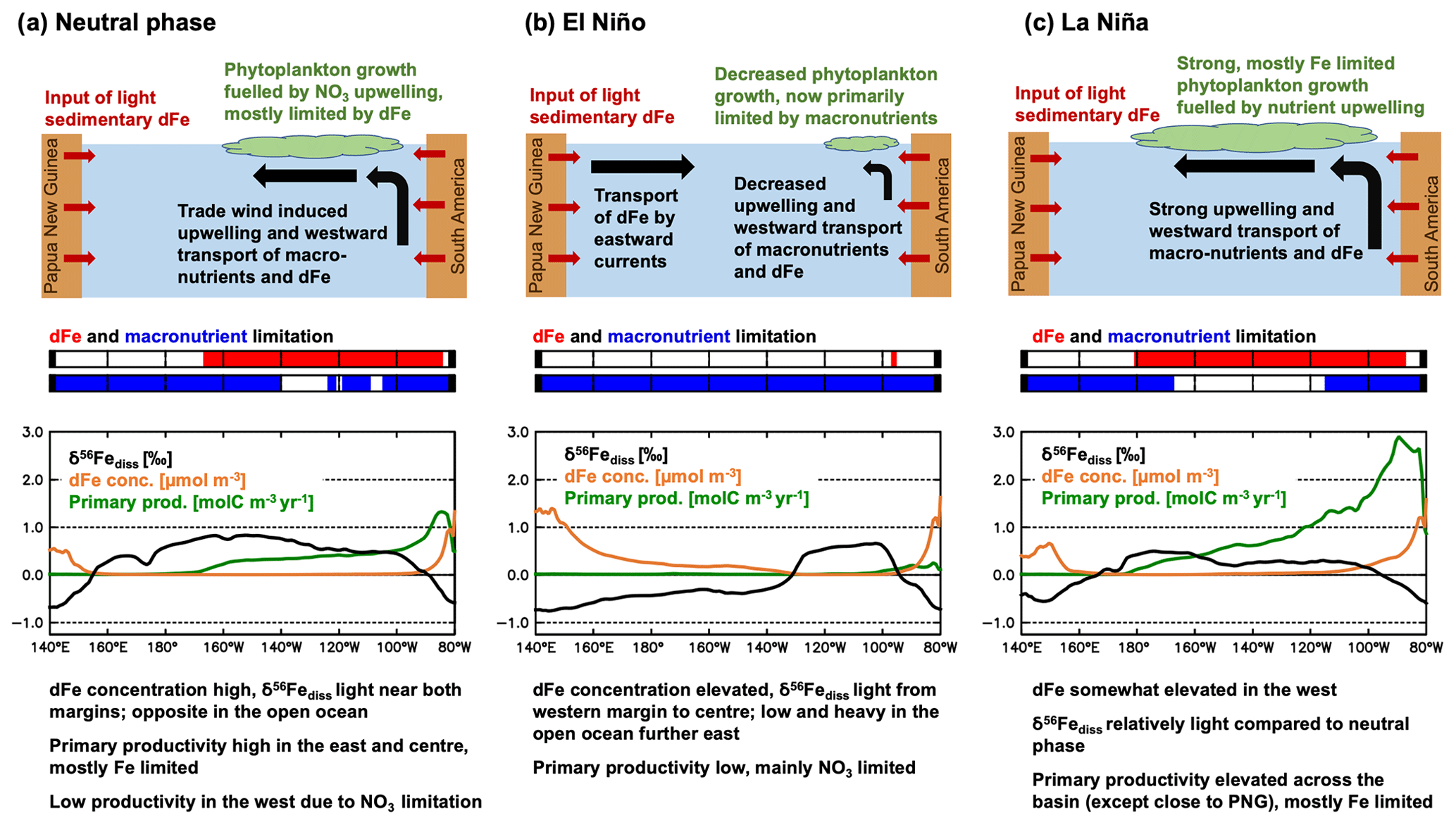
Figure 4Overview of processes behind δ56Fediss changes in the equatorial Pacific during an El Niño/La Niña cycle. Note that the example δ56Fediss (‰), dFe concentration (µmol m−3), and primary productivity (molC m−3 yr−1) curves were taken from the same months as in Fig. 5, i.e. July 1996 for neutral, December 1997 for El Niño, and December 1998 for La Niña phases, using average values from 5∘ S to 5∘ N. The dFe and macronutrient limitation plots were taken from the same months and indicate if dFe (red) or macronutrients are limiting phytoplankton growth in (parts of) the 5∘ S to 5∘ N region.
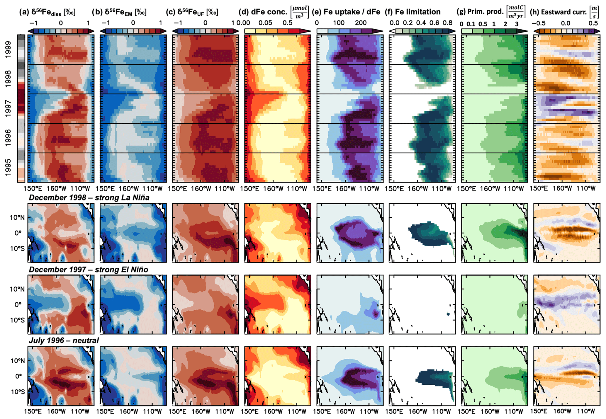
Figure 5Mechanisms behind surface ocean δ56Fediss changes in the equatorial Pacific from the hindcast experiment during a strong El Niño/La Niña cycle. Upper half: time series (1995–1999; from hindcast experiments) of monthly mean surface ocean (a) δ56Fediss (‰), (b) δ56FeUF (‰), (c) δ56FeUF (‰), (d) dFe concentration (µmol m−3), (e) ratio of Fe uptake to dFe concentration, (f) Fe limitation, (g) primary productivity (molC m−3 yr−1), and (d) upper ocean (0–50 m average) eastward currents (m s−1), averaged from 5∘ N to 5∘ S. The Ocean Niño Index is included on the left (red: El Niño, grey: La Niña). Lower half: map view of the same parameters in July 1996 (neutral), December 1997 (strong El Niño), December 1998 (strong La Niña).
The reversal of upper ocean currents during El Niño/La Niña cycles has a direct impact on δ56FeEM. In neutral phases before the on-set of El Niño (e.g. July 1996), waters with elevated dFe concentration are upwelled at the South American margin and transported westward (Fig. 5d, h). The δ56Fe endmember signature of this dFe is light, as it is mostly sourced from reducing sediments at the South American margin (Fig. 5b). As the currents reverse during an El Niño event such as in 1997, the upwelling and transport at the eastern margin is reduced and instead, high dFe waters with light δ56FeEM from margin sediments in the PNG region are preferentially transported eastwards (Fig. 5b, d). Thus, δ56FeEM is light in the west but remains near a crustal signature (i.e. ca. 0.1 ‰) in the eastern tropical Pacific, where the main source of external dFe is now dust deposition. Finally, as the El Niño conditions collapse and La Niña develops (as in 1998), strong westward currents lead to a similar, but larger, light δ56FeEM anomaly from the South American margin as in the neutral phase, which, in the case of the strong El Niño/La Niña cycle of 1997/1998, extends across the basin (Fig. 5b). Note that the sedimentary Fe input from the PNG region may not be as isotopically light as suggested by our model so that the endmember effects in the western part of the basin may be reduced, as discussed in Sect. 4.1. Also, the sedimentary Fe supply from the PNG region to the equatorial undercurrent (EUC) may be underestimated in our model compared to some (but not all) of the available regional observations (Fig. S7). As the EUC supplies Fe to the surface ocean (e.g. Coale et al., 1996; Kaupp et al., 2011), this may cause additional impacts on surface ocean dFe concentrations and δ56Fediss as well as their response to climate variability, which affects the strength of the EUC (e.g. Firing et al., 1983; Johnson et al., 2000).
The impact of circulation changes associated with the El Niño/La Niña cycle on δ56FeUF depends on the ratio of Fe uptake to dFe concentrations. Impacts of El Niño/La Niña on uptake fractionation integrate the changes in primary production, limiting nutrients, and, consequently, Fe uptake rates by phytoplankton. Uptake fractionation becomes strongest in our model when Fe uptake rates are high relative to dFe concentrations (Fig. 5e). This leads to heavy δ56FeUF. When the ratio of Fe uptake to dFe concentration is high, the system is usually Fe limited (Fig. 5f). During the neutral phases such as in summer 1996, such “high Fe uptake, low dFe concentration” conditions with heavy δ56FeUF are prevalent in the central and eastern tropical Pacific (Fig. 5c, e), which are relatively productive and strongly Fe limited (Fig. 5f, g). As El Niño develops, the decreased upwelling and westward transport of macronutrients (e.g. nitrate) from the South American margin leads to a decrease in productivity and a switch from Fe to nitrogen limitation in the central and eastern Pacific (Fig. 5f, g). When combined with the input of dFe from the western margin, this shift of nutrient limitation leads to low ratios of Fe uptake to dFe concentration (Fig. 5e), and therefore lower uptake fractionation effects (i.e. relatively light δ56FeUF) across the basin. During the following La Niña, dFe concentrations are relatively high in the Fe-limited eastern and central Pacific (Fig. 5d). These elevated dFe concentrations are due to decreased Fe uptake during the nitrogen-limited El Niño phase and the increased westward transport of dFe from the South American margin during La Niña. Consequently, the ratio of Fe uptake to dFe concentration is relatively low and uptake fractionation effects moderate (Fig. 5c, e), despite high primary productivity fuelled by the increased upwelling of nitrate and dFe (Fig. 5g).
3.2.3 Future (2006–2100) δ56Fediss variability in the tropical Pacific driven by climate change
The climate change-induced decrease in surface ocean δ56Fediss variability in the western equatorial Pacific and increase in the eastern equatorial Pacific over the next century, shown in Fig. 2, is driven by decreased upwelling of cold water in the east (Figs. S8, 6, 7). This reduces the input and westward transport of both macronutrients and isotopically light sedimentary dFe from the South American margin to the surface ocean and decreases primary production. These changes are all similar to those occurring during El Niño events from our hindcast simulations. Consequently, the western half of the equatorial Pacific becomes nitrogen limited and primary productivity is low, leading to roughly constant uptake fractionation, i.e. invariable δ56FeUF. Conversely, the effects of different ENSO phases are now concentrated in the eastern equatorial Pacific, where variability is high for both δ56FeEM and δ56FeUF, due to changes in upwelling of light dFe and variability in the degree of Fe limitation (or switches to nitrogen limitation) respectively.
Importantly, circulation patterns during the historical period (1852–2005) in the climate change simulations are not as realistic as for the hindcast experiments, which were forced by an atmospheric reanalysis. For instance, the cold SST anomaly at the Equator is too strong and extends too far west in the climate change simulations, which is a common bias in such climate models (e.g. Planton et al., 2021). This “cold tongue bias” is caused by upwelling in the eastern Pacific which is too strong in the historical era of climate change experiment. This is also evident when comparing the equatorial SST of the climate change and hindcast simulations and is likely also responsible for the lower δ56FeEM variability in the western tropical Pacific in the climate change simulation (Fig. S8). In addition, there is some disagreement between observations and the ENSO cycles produced by the climate change model (in the historical period of 1982–2005), for instance, regarding seasonal timing and zonal pattern (Bellenger et al., 2014; Planton et al., 2021). As models which better agree with historical ENSO characteristics predict the frequency of extreme ENSO events to increase (Cai et al., 2015, 2021), future variability in δ56Fediss may be higher than predicted by our climate change experiment.
While the physical model shows some biases in terms of SST and ENSO characteristics, the modelled primary productivity changes in the tropical Pacific in response to changing SST during ENSO cycles agree well with available constraints from SST observations and satellite estimates of primary production (Kwiatkowski et al., 2017; Tagliabue et al., 2020). This strengthens our confidence in the effect of ENSO cycles on δ56FeUF, as it indicates that the impact of the different ENSO phases on the model biogeochemistry is realistic. It should be noted that the physical setting of the climate change experiments is based on model simulations using the high-emissions RCP8.5 scenario. As smaller changes in biogeochemical and physical conditions are predicted for lower emission scenarios (Dufresne et al., 2013; Kwiatkowski et al., 2020), we would expect the δ56Fediss changes also to be reduced in parallel.
3.3 Impact of climate change on surface ocean δ56Fediss in the Southern Hemisphere
Future climate change-induced alterations to δ56Fediss become largest in the Southern Hemisphere. The largest changes occur in a region between about 30 and 50∘ S (Figs. 2, 6a), where stronger uptake fractionation effects (i.e. heavier δ56FeUF; Fig. 6b) lead to increasingly heavy δ56Fediss in the Pacific and Indian oceans (Fig. 6a). These changes in uptake fractionation are ultimately caused by higher primary production rates (Fig. 7c), which lead to stronger Fe limitation (Fig. 7b) and thus higher δ56FeUF (Fig. 6b). The increases in δ56FeUF between 30 and 50∘ S are reinforced by an increase in δ56FeEM in the western parts of each basin (Fig. 6c) due to a southward shift of low dFe areas with relatively heavy δ56FeEM (Figs. 6c, 7a). Conversely, the δ56Fediss decrease at lower latitudes is due to lower primary productivity and Fe limitation (Fig. 7b, c), and thus lighter δ56FeUF (Fig. 6b). A notable decrease in δ56Fediss thereby occurs just north of the heavy δ56Fediss area due to a decrease in Fe limitation as the region of high, Fe-limited primary productivity moves southward. Similarly, the strong decrease in δ56FeUF (and thus δ56Fediss) in the South Atlantic is due to a decrease in Fe limitation and, in some parts, a shift to macronutrient limitation. Many of the changes in dFe and NO3 concentration, primary productivity, and Fe limitation (Fig. 6) that drive δ56Fediss changes over the next century were also observed in the only other available study on the impact of climate change on the ocean Fe cycle (Misumi et al., 2014). For instance, these authors also report increased future primary productivity at around 40∘ S, which is Fe limited in the Indian and Pacific but no longer in the Atlantic (Misumi et al., 2014). The slight difference in depth range and time periods used in Fig. 6 in this study relative to those reported by Misumi et al. (2014) has little impact on the trends of each parameter. One major difference between the two simulations concerns primary productivity in the eastern tropical Pacific, which is predicted to decrease in our model, due to a switch from Fe to NO3 limitation, but increases in the simulation of Misumi et al. (2014), in which phytoplankton remain mostly Fe limited (see also Sect. 4.2 and Tagliabue et al., 2020).
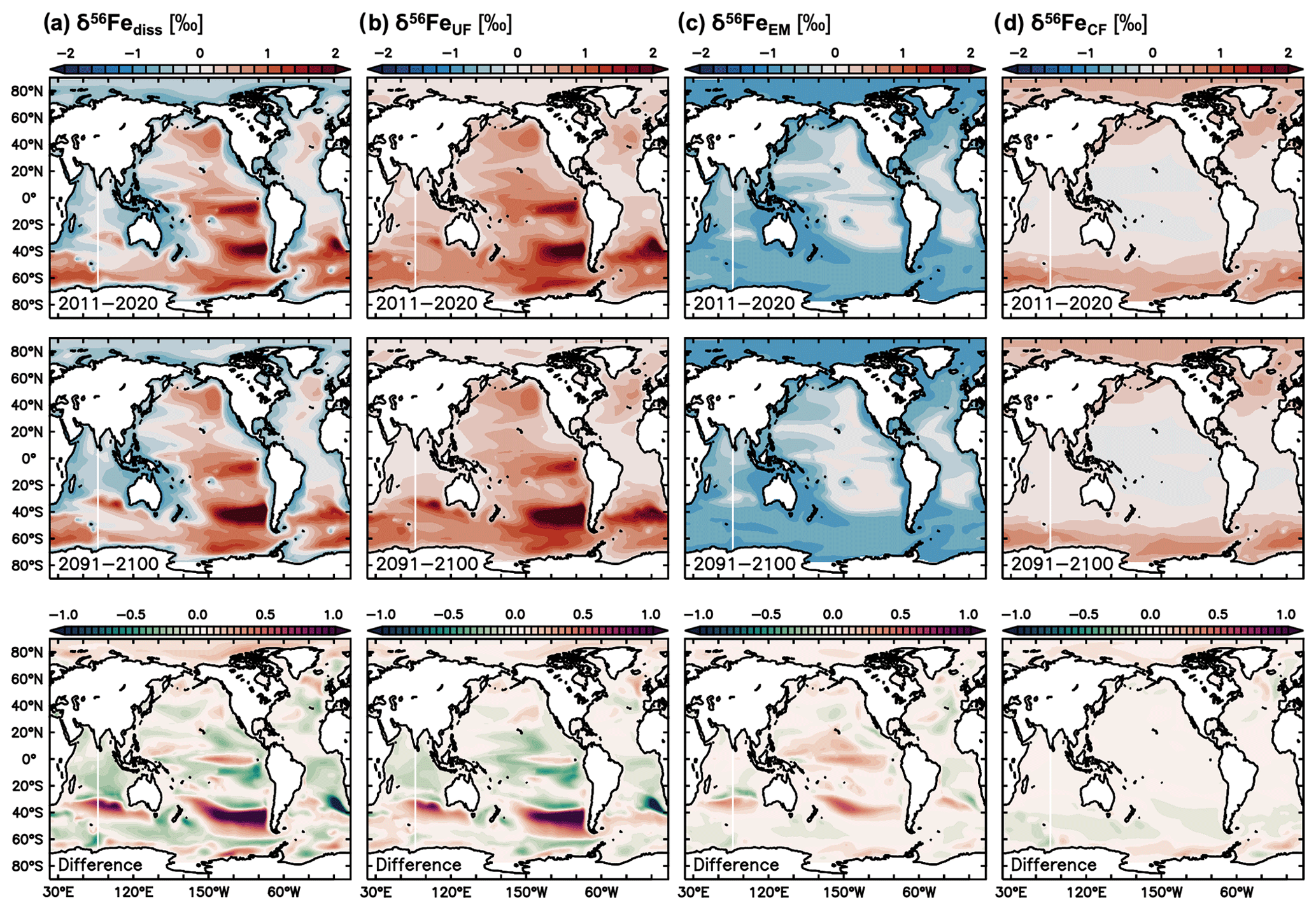
Figure 6Climate change effect on δ56Fediss and its drivers. Present decade (2011–2020 average) and end-of-century (2091–2100 average) climate change simulation values of (a) δ56Fediss (‰), (b) δ56FeUF (‰), (c) δ56FeEM (‰), and (d) δ56FeUF (‰). The difference in future minus present values is shown in the bottom row.
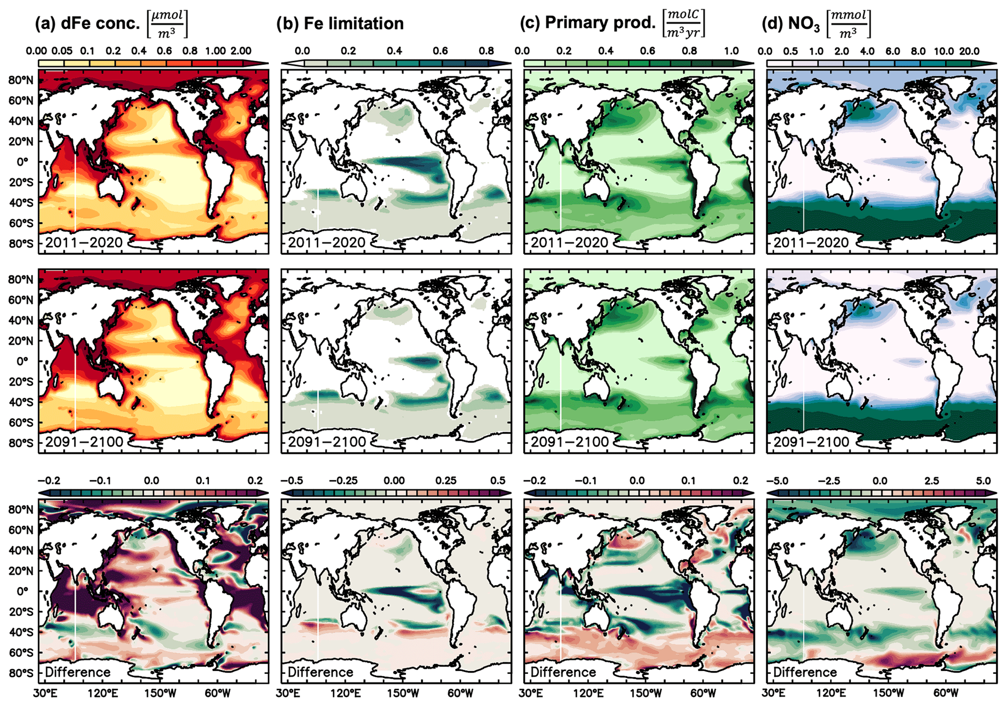
Figure 7Climate change effect on underlying mechanisms of δ56Fediss drivers. Present decade (2011–2020 average) and end-of-century (2091–2100 average) climate change simulation values of (a) dFe concentration (µmol m−3), (b) Fe limitation, (c) primary production (molC m−3 yr−1), and (d) nitrate (mmol m−3). The difference in future minus present values is shown in the bottom row.
The δ56Fediss decrease in some higher-latitude areas (around ca. 60∘ S) is driven by a higher concentration of dFe, likely due to redistribution of “new” dFe from external sources. This is consistent with the slight decrease in δ56FeEM and the lower δ56FeCF, which is generally characteristic of “younger” water (Fig. 6c, d; König et al., 2021). Such increases in dFe concentrations also lower the δ56FeUF effect (Fig. 6b), as the Fe uptake to dFe concentration ratio has decreased.
As discussed above, Fe isotopes have been used in the past to track both external Fe sources and internal cycling. Here, we demonstrated how both historical and future surface ocean δ56Fediss variability arises from a combination of the redistribution of “new” Fe from external sources and changes to internal cycling, especially Fe uptake by phytoplankton under Fe limiting conditions. This raises the question as to whether observed variations in δ56Fediss can be used to infer alterations in external Fe distribution and Fe uptake and limitation.
4.1 Using δ56Fediss to track changes in input of new Fe from external sources
Variability in surface ocean δ56Fediss in the tropical Pacific is a great example of how δ56Fediss may track new Fe input from external sources. Here, δ56FeEM is likely responsible for a substantial fraction of δ56Fediss variability (Figs. 1f, 2d) and tracks ENSO-related circulation changes that redistribute Fe zonally from different external sources (Sect. 3.2). Specifically, the eastward transport of isotopically light Fe from PNG sediments during El Niño events and the westward transport of light Fe from Peru sediments are discernible as light δ56FeEM (and δ56Fediss) anomalies in the respective regions (Fig. 3c, d). Simultaneous eastward and westward shifts in the open ocean region that receives most dust Fe input are also evident based on their more crustal δ56FeEM (Fig. 3d).
Tracking external Fe input using δ56Fediss is sensitive to the choice of δ56Fe endmembers for the different (potential) new Fe sources. This has been discussed previously in a range of studies (e.g. Conway and John, 2014; König et al., 2022; Pinedo-González et al., 2020). For instance, in the tropical Pacific our model includes major new Fe inputs from continental margins, with this sedimentary-sourced Fe being isotopically light, with a δ56Fe endmember of −1 ‰ in the upper ca. 400 m (as it is assumed to be released by reductive dissolution at these depths independent of location; König et al., 2021). Input of such light δ56Fediss appears to be realistic for the eastern margin, as light δ56Fediss have been observed in the Peru upwelling region (Chever et al., 2015; Fitzsimmons et al., 2016; John et al., 2018). However, isotopically heavier dFe has been observed in the western and central tropical Pacific and has been suggested to be released from PNG sediments via non-reductive processes with crustal (ca. 0.1 ‰) δ56Fe endmembers (Labatut et al., 2014; Radic et al., 2011). A sensitivity test with neutral (0 ‰) sediment δ56Fe endmember shows that, without any light sedimentary Fe input, δ56FeEM variability and, consequently, δ56Fediss variability are reduced in the surface ocean (Fig. S9). This consequently increases the dominance of fractionation effects (mainly δ56FeUF; Fig. S9). Thus, in areas such as the western tropical Pacific and areas further east which receive Fe from the EUC (Sect. 3.2.2), δ56FeEM variability may be reduced, as the modelled sediment Fe input from the PNG margin is too light. A greater extent of non-reductive Fe input would mean that changes in new Fe input or redistribution by ocean circulation would be harder to detect using δ56Fediss. This is especially true in areas where fractionation effects are strong and thereby conceal changes in δ56FeEM. On the other hand, δ56Fediss could be useful to track new Fe input and redistribution in areas such as the eastern tropical Pacific, where the δ56Fe endmember of new Fe is observed to be light, and where δ56FeEM is responsible for a substantial part of δ56Fediss variability.
Another complicating factor for tracking Fe input changes with δ56Fediss is when fractionation and endmember effects overlap each other. Most fractionating processes lead to heavier δ56Fediss in our model (except for colloidal pumping; König et al., 2021), whereas endmember effects are comparably light, even for dust Fe or Fe from non-reductive sediments with crustal δ56Fe. Thus, if fractionation effects (δ56FeUF and/or δ56FeCF) do not vary in unison with δ56FeEM, changes in Fe input may be hidden (as illustrated for the North Pacific in Fig. S3). However, where variability in fractionation and endmember effects occur simultaneously, fractionation effects may reinforce δ56FeEM variability (Fig. S3). This is mostly the case in the tropical Pacific, especially at the Equator (Fig. S6), with some discrepancies in the central Pacific south of the Equator (Fig. S3). Here, changes in the redistribution of external Fe could even be deducted from δ56FeUF alone.
In summary, it is necessary to have a good grasp on the relevant δ56Fe endmembers when inferring changes in external Fe input or redistribution from δ56Fediss, as well as understanding variability in δ56FeUF and δ56FeCF relative to δ56FeEM (Fig. S3). Such changes are therefore easiest to spot where the external Fe source in question is known to provide isotopically light Fe and where fractionation effects are weak and/or invariable in time.
4.2 Using δ56Fediss to track changes in Fe limitation and recycled Fe
Areas of strong Fe limitation are generally associated with heavy δ56Fediss driven by strong uptake fractionation effects (i.e. heavy δ56FeUF), often reinforced by relatively heavy δ56FeEM due to limited input of light Fe from external sources (Sect. 3.2, 3.3). This suggests that heavy δ56Fediss could be a potentially useful indicator of Fe limitation, which opens up the possibility of detecting or even monitoring changes in Fe limitation using δ56Fediss. Such information would be valuable, since Fe is thought to limit primary production in large parts of the global ocean (Moore et al., 2013). However, the specific extent of Fe limitation is unknown and may vary over seasonal, interannual, and decadal timescales. Poorly constrained climate change-driven changes in Fe limitation have been demonstrated to explain large parts of the uncertainty in model projections of net primary production (NPP) in the tropical Pacific, where future NPP is predicted to depend decisively on whether or not phytoplankton switch from Fe to NO3 limitation (Tagliabue et al., 2020; see also Sect. 3.3).
Outputs from our hindcast experiments show that the connection between heavy surface ocean δ56Fediss and Fe limitation generally holds and that seasonal changes in Fe limitation are tracked by δ56FeUF and, consequently, δ56Fediss (Fig. S10). As discussed for the tropical Pacific (Sect. 3.2), this is due to the fact that uptake fractionation is strongest (i.e. δ56FeUF heaviest) where the ratio of Fe uptake to dFe concentration is highest; this ratio also determines the degree of Fe limitation (where Fe is the limiting nutrient; Figs. 3, S5). However, in some regions, namely in the south and south-eastern Pacific, δ56FeUF (and δ56Fediss) can be heavy despite a relatively moderate ratio of Fe uptake to dFe concentration (Fig. S10), and δ56FeUF variability appears to be anti-correlated to Fe limitation patterns (Fig. S3). While we cannot rule out that the heavy δ56FeUF is caused by model artefacts, it may also be related to the ocean circulation pattern of these areas. In contrast to the equatorial Pacific, where ENSO dynamics supply water with light δ56Fediss every few years, much of the water in the southeast Pacific originates in the seasonally Fe-limited Southern Ocean and contains Fe with relatively heavy δ56Fediss (Fig. S10). Here, the heavy δ56Fediss therefore might not (only) be caused by local processes but could be mostly a “legacy” signature. It may also indicate that this dFe has been continuously recycled by phytoplankton on its way to the south-east Pacific. Such recycling would leave dFe isotopically heavy given the preferential uptake of light Fe in our model (Sect. 2), as parts of the (isotopically lighter) phytoplankton Fe are removed from the surface ocean via particle settling. When deriving the local degree of Fe limitation from δ56Fediss, it is therefore important to consider the “background” δ56Fediss based on the origin of dFe and previous processing. Moreover, local δ56FeEM effects should also be considered, especially if they are variable in time and space.
As discussed above, the connection between heavy δ56Fediss and Fe limitation is a consequence of the uptake fractionation parametrization of our model. For this parametrization we use a constant fractionation factor (α = 0.9995) for Fe uptake by both phytoplankton classes, based on observations from an Fe-limited Southern Ocean eddy (Ellwood et al., 2020). Thus, the uptake fractionation strength is independent of factors such as dFe concentration, temperature, or species composition. This is in contrast to uptake of other nutrients such as ammonium, for which fractionation was found to decrease when concentrations were low (Sigman and Fripiat, 2019). While it is conceivable that δ56Fe fractionation during phytoplankton uptake is impacted by dFe availability and/or other parameters, observational studies on the topic are limited. Exceedingly heavy surface ocean δ56Fediss values have been observed in multiple, likely Fe-limited, systems (e.g. in the eastern tropical Pacific, Southern Ocean, South Atlantic; Fig. S10); for some of these systems, the heavy δ56Fediss has indeed been attributed to continuous biological processing (i.e. uptake and recycling) combined with fractionation during organic complexation (Ellwood et al., 2020; Sieber et al., 2021). This supports the concentration-independent uptake fractionation of our model since heavy surface ocean δ56Fediss would not emerge in model simulations if uptake fractionation was set to decrease for low dFe. Nevertheless, more observational or, ideally, experimental data are necessary to determine which factors may impact uptake fractionation and to find the appropriate fractionation factor parametrizations.
Overall, heavy δ56Fediss could be a useful indicator of Fe limitation if complicating factors such as past processing and variable δ56FeEM are taken into account. Fe limitation derived from δ56Fediss observations could thereby complement other measures of nutrient limitation, such as the (scarce) limitation data from incubation experiments (Moore et al., 2013) or the limitation inferred from nutrient deficiencies (Moore, 2016). Our modelling results suggest that changes in Fe limitation can induce strong seasonal variability in δ56Fediss in some locations (this study, König et al., 2022) but also variability over interannual and decadal scales. Thus, it would be worthwhile to observe δ56Fediss changes over seasonal and interannual timescales in the form of a δ56Fediss time series, ideally in a place with variable (degrees of) Fe limitation. A possible candidate location could be the Southern Ocean Time Series (140∘ E, 47∘ S), which is Fe limited in summer (Boyd et al., 2001; Sedwick et al., 1999). Here, our model predicts substantial seasonal variability in surface ocean δ56Fediss (between ca. 0.1 ‰ and 0.7 ‰); available observations are within this range (Barrett et al., 2021; Ellwood et al., 2020). Moreover, based on predicted present and future variability in Fe limitation and, consequently, δ56Fediss in our model (Figs. 1–2), the equatorial and south-eastern Pacific could be potential locations for future studies that explore the interannual changes in iron limitation.
Simulations of a global ocean model with an active δ56Fe cycle and variable climate forcings show that surface ocean δ56Fediss responds distinctly to the changes in ocean physics and biogeochemistry triggered by natural climate variability and long-term global warming effects. Changes in δ56Fediss thereby integrate both variations in external Fe supply and redistribution and shifts in upper ocean biogeochemistry (especially presence and degree of Fe limitation), which alter δ56Fe endmember and uptake fractionation effects respectively. We therefore suggest that regular observations of surface ocean δ56Fediss as part of a long-term time series could be useful to track climate-driven changes to upper ocean Fe supply or the degree of Fe limitation in phytoplankton. As endmember and fractionation effects can overlap, δ56Fediss and dFe concentration data should ideally be accompanied by ancillary measurements to constrain changes in upper ocean circulation or primary productivity. In areas with high seasonal variability in δ56Fediss (e.g. due to strong seasonality in primary productivity), a sub-annual sampling interval should be considered.
Model outputs are available from https://doi.org/10.5281/zenodo.7418726 (König and Tagliabue, 2022).
The supplement related to this article is available online at: https://doi.org/10.5194/bg-20-4197-2023-supplement.
DK and AT designed the study. DK adapted the model set-up, ran simulations, analysed model outputs, and drafted the article with support from AT. All authors contributed to article editing and revision.
The contact author has declared that neither of the authors has any competing interests.
Publisher’s note: Copernicus Publications remains neutral with regard to jurisdictional claims in published maps and institutional affiliations.
This work was undertaken on Barkla, part of the High Performance Computing facilities at the University of Liverpool, UK. We acknowledge the GTMBA Project Office of NOAA/PMEL for providing the TAO/TRITON moored buoy array dataset.
This research has been supported by the European Research Council (ERC) under the European Union (grant no. 724289).
This paper was edited by Peter Landschützer and reviewed by two anonymous referees.
Aumont, O., Ethé, C., Tagliabue, A., Bopp, L., and Gehlen, M.: PISCES-v2: an ocean biogeochemical model for carbon and ecosystem studies, Geosci. Model Dev., 8, 2465–2513, https://doi.org/10.5194/gmd-8-2465-2015, 2015.
Aumont, O., van Hulten, M., Roy-Barman, M., Dutay, J.-C., Éthé, C., and Gehlen, M.: Variable reactivity of particulate organic matter in a global ocean biogeochemical model, Biogeosciences, 14, 2321–2341, https://doi.org/10.5194/bg-14-2321-2017, 2017.
Barrett, P. M., Grun, R., and Ellwood, M. J.: Tracing iron along the flowpath of East Australian Current using iron stable isotopes, Mar. Chem., 237, 104039, https://doi.org/10.1016/j.marchem.2021.104039, 2021.
Bellenger, H., Guilyardi, E., Leloup, J., Lengaigne, M., and Vialard, J.: ENSO representation in climate models: From CMIP3 to CMIP5, Clim. Dynam., 42, 1999–2018, https://doi.org/10.1007/s00382-013-1783-z, 2014.
Bindoff, N. L., Cheung, W. W., Kairo, J. G., Arístegui, J., Guinder, V. A., Hallberg, R., Hilmi, N., Jiao, N., Karim, M. S., Levin, L., O'Donoghue, S., Cuicapusa, S. R. P., Rinkevich, B., Suga, T., Tagliabue, A., and Williamson, P.: Changing Ocean, Marine Ecosystems, and Dependent Communities, in: IPCC Special Report on the Ocean and Cryosphere in a Changing Climate, edited by: Pörtner, H.-O., Roberts, D. C., Masson-Delmotte, V., Zhai, P., Tignor, M., Poloczanska, E., Mintenbeck, K., Alegría, A., Nicolai, M., Okem, A., Petzold, J., Rama, B., and Weyer, N. M., 447–587, Cambridge University Press, https://doi.org/10.1017/9781009157964.007, 2019.
Bonnet, S. and Guieu, C.: Atmospheric forcing on the annual iron cycle in the western Mediterranean Sea: A 1-year survey, J. Geophys. Res.-Oceans, 111, 1–13, https://doi.org/10.1029/2005JC003213, 2006.
Boyd, P. W. and Ellwood, M. J.: The biogeochemical cycle of iron in the ocean, Nat. Geosci., 3, 675–682, https://doi.org/10.1038/ngeo964, 2010.
Boyd, P. W., Crossley, A. C., DiTullio, G. R., Griffiths, F. B., Hutchins, D. A., Queguiner, B., Sedwick, P. N., and Trull, T. W.: Control of phytoplankton growth by iron supply and irradiance in the subantarctic Southern Ocean: Experimental results from the SAZ Project, J. Geophys. Res.-Oceans, 106, 31573–31583, https://doi.org/10.1029/2000jc000348, 2001.
Buchanan, P. J. and Tagliabue, A.: The Regional Importance of Oxygen Demand and Supply for Historical Ocean Oxygen Trends, Geophys. Res. Lett., 48, e2021GL094797, https://doi.org/10.1029/2021GL094797, 2021.
Cai, W., Santoso, A., Wang, G., Yeh, S. W., An, S. Il, Cobb, K. M., Collins, M., Guilyardi, E., Jin, F. F., Kug, J. S., Lengaigne, M., Mcphaden, M. J., Takahashi, K., Timmermann, A., Vecchi, G., Watanabe, M., and Wu, L.: ENSO and greenhouse warming, Nat. Clim. Change, 5, 849–859, https://doi.org/10.1038/nclimate2743, 2015.
Cai, W., Santoso, A., Collins, M., Dewitte, B., Karamperidou, C., Kug, J.-S. S., Lengaigne, M., McPhaden, M. J., Stuecker, M. F., Taschetto, A. S., Timmermann, A., Wu, L., Yeh, S.-W. W., Wang, G., Ng, B., Jia, F., Yang, Y., Ying, J., Zheng, X.-T. T., Bayr, T., Brown, J. R., Capotondi, A., Cobb, K. M., Gan, B., Geng, T., Ham, Y.-G., Jin, F.-F., Jo, H.-S., Li, X., Lin, X., McGregor, S., Park, J.-H., Stein, K., Yang, K., Zhang, L., and Zhong, W.: Changing El Niño–Southern Oscillation in a warming climate, Nat. Rev. Earth Environ., 2, 628–644, https://doi.org/10.1038/s43017-021-00199-z, 2021.
Chever, F., Rouxel, O. J., Croot, P. L., Ponzevera, E., Wuttig, K., and Auro, M. E.: Total dissolvable and dissolved iron isotopes in the water column of the Peru upwelling regime, Geochim. Cosmochim. Ac., 162, 66–82, https://doi.org/10.1016/j.gca.2015.04.031, 2015.
Coale, K. H., Fitzwater, S. E., Gordon, R. M., Johnson, K. S., and Barber, R. T.: Control of community growth and export production by upwelled iron in the equatorial Pacific Ocean, Nature, 379, 621–624, https://https://doi.org/10.1038/379621a0, 1996.
Conway, T. M. and John, S. G.: Quantification of dissolved iron sources to the North Atlantic Ocean, Nature, 511, 212–215, https://doi.org/10.1038/nature13482, 2014.
Conway, T. M., John, S. G., and Lacan, F.: Intercomparison of dissolved iron isotope profiles from reoccupation of three GEOTRACES stations in the Atlantic Ocean, Mar. Chem., 183, 50–61, https://doi.org/10.1016/j.marchem.2016.04.007, 2016.
Conway, T. M., Hamilton, D. S., Shelley, R. U., Aguilar-Islas, A. M., Landing, W. M., Mahowald, N. M., and John, S. G.: Tracing and constraining anthropogenic aerosol iron fluxes to the North Atlantic Ocean using iron isotopes, Nat. Commun., 10, 2628, https://doi.org/10.1038/s41467-019-10457-w, 2019.
Dufresne, J. L., Foujols, M. A., Denvil, S., Caubel, A., Marti, O., Aumont, O., Balkanski, Y., Bekki, S., Bellenger, H., Benshila, R., Bony, S., Bopp, L., Braconnot, P., Brockmann, P., Cadule, P., Cheruy, F., Codron, F., Cozic, A., Cugnet, D., de Noblet, N., Duvel, J.-P., Ethé, C., Fairhead, L., Fichefet, T., Flavoni, S., Friedlingstein, P., Grandpeix, J.-Y., Guez, L., Guilyardi, E., Hauglustaine, D., Hourdin, F., Idelkadi, A., Ghattas, J., Joussaume, S., Kageyama, M., Krinner, G., Labetoulle, S., Lahellec, A., Lefebvre, M.-P., Lefevre, F., Levy, C., Li, Z. X., Lloyd, J., Lott, F., Madec, G., Mancip, M., Marchand, M., Masson, S., Meurdesoif, Y., Mignot, J., Musat, I., Parouty, S., Polcher, J., Rio, C., Schulz, M., Swingedouw, D., Szopa, S., Talandier, C., Terray, P., Viovy, N., and Vuichard, N.: Climate change projections using the IPSL-CM5 Earth System Model: From CMIP3 to CMIP5, Clim. Dynam., 40, 2123–2165, https://doi.org/10.1007/s00382-012-1636-1, 2013.
Ellwood, M. J., Hutchins, D. A., Lohan, M. C., Milne, A., Nasemann, P., Nodder, S. D., Sander, S. G., Strzepek, R. F., Wilhelm, S. W., and Boyd, P. W.: Iron stable isotopes track pelagic iron cycling during a subtropical phytoplankton bloom, P. Natl. Acad. Sci. USA, 112, E15–E20, https://doi.org/10.1073/pnas.1421576112, 2015.
Ellwood, M. J., Strzepek, R. F., Strutton, P. G., Trull, T. W., Fourquez, M., and Boyd, P. W.: Distinct iron cycling in a Southern Ocean eddy, Nat. Commun., 11, 825, https://doi.org/10.1038/s41467-020-14464-0, 2020.
Firing, E., Lukas, R., Sadler, J., and Wyrtki, K.: Equatorial undercurrent disappears during 1982–1983 El Niño, Science, 222, 1121–1123, https://https://doi.org/10.1126/science.222.4628.1121, 1983.
Fitzsimmons, J. N., Conway, T. M., Lee, J. M., Kayser, R., Thyng, K. M., John, S. G., and Boyle, E. A.: Dissolved iron and iron isotopes in the southeastern Pacific Ocean, Global Biogeochem. Cy., 30, 1372–1395, https://doi.org/10.1002/2015GB005357, 2016.
Fitzsimmons, J. N., Hayes, C. T., Al-Subiai, S. N., Zhang, R., Morton, P. L., Weisend, R. E., Ascani, F., and Boyle, E. A.: Daily to decadal variability of size-fractionated iron and iron-binding ligands at the Hawaii Ocean Time-series Station ALOHA, Geochim. Cosmochim. Ac., 171, 303–324, https://doi.org/10.1016/j.gca.2015.08.012, 2015.
Homoky, W. B., Severmann, S., Mills, R. A., Statham, P. J., and Fones, G. R.: Pore-fluid Fe isotopes reflect the extent of benthic Fe redox recycling: Evidence from continental shelf and deep-sea sediments, Geology, 37, 751–754, https://doi.org/10.1130/G25731A.1, 2009.
Homoky, W. B., John, S. G., Conway, T. M., and Mills, R. A.: Distinct iron isotopic signatures and supply from marine sediment dissolution, Nat. Commun., 4, 2143, https://doi.org/10.1038/ncomms3143, 2013.
John, S. G., Helgoe, J., Townsend, E., Weber, T., DeVries, T., Tagliabue, A., Moore, J. K., Lam, P. J., Marsay, C. M., and Till, C. P.: Biogeochemical cycling of Fe and Fe stable isotopes in the Eastern Tropical South Pacific, Mar. Chem., 201, 66–76, https://doi.org/10.1016/j.marchem.2017.06.003, 2018.
Johnson, K. S., Chavez, F. P., and Friederich, G. E.: Continentalshelf sediment as a primary source of iron for coastal phytoplankton, Nature, 398, 697–700, https://doi.org/10.1038/19511, 1999.
Johnson, G. C., McPhaden, M. J., Rowe, G. D., and McTaggart, K. E.: Upper equatorial Pacific Ocean current and salinity variability during the 1996–1998 El Niño-La Niña cycle, J. Geophys. Res.-Oceans, 105, 1037–1053, https://https://doi.org/10.1029/1999jc900280, 2000.
Johnson, K. S., Chavez, F. P., and Friederich, G. E.: Continental-shelf sediment as a primary source of iron for coastal phytoplankton, Nature, 398, 697–700, https://doi.org/10.1038/19511, 1999.
Kaupp, L. J., Measures, C. I., Selph, K. E., and Mackenzie, F. T.: The distribution of dissolved Fe and Al in the upper waters of the Eastern Equatorial Pacific, Deep-Sea Res. Pt. II, 58, 296–310, https://doi.org/10.1016/j.dsr2.2010.08.009, 2011.
König, D. and Tagliabue, A.: The Fingerprint of Climate Variability on the Surface Ocean Cycling of Iron and its Isotopes, Zenodo [data set], https://doi.org/10.5281/zenodo.7418726, 2022.
König, D., Conway, T. M., Ellwood, M. J., Homoky, W. B., and Tagliabue, A.: Constraints on the Cycling of Iron Isotopes From a Global Ocean Model, Global Biogeochem. Cy., 35, e2021GB006968, https://doi.org/10.1029/2021GB006968, 2021.
König, D., Conway, T. M., Hamilton, D. S., and Tagliabue, A.: Surface Ocean Biogeochemistry Regulates the Impact of Anthropogenic Aerosol Fe Deposition on the Cycling of Iron and Iron Isotopes in the North Pacific, Geophys. Res. Lett., 49, e2022GL098016, https://doi.org/10.1029/2022GL098016, 2022.
Kurisu, M., Adachi, K., Sakata, K., and Takahashi, Y.: Stable Isotope Ratios of Combustion Iron Produced by Evaporation in a Steel Plant, ACS Earth Space Chem., 3, 588–598, https://doi.org/10.1021/acsearthspacechem.8b00171, 2019.
Kwiatkowski, L., Bopp, L., Aumont, O., Ciais, P., Cox, P. M., Laufkötter, C., Li, Y., and Séférian, R.: Emergent constraints on projections of declining primary production in the tropical oceans, Nat. Clim. Change, 7, 355–358, https://doi.org/10.1038/nclimate3265, 2017.
Kwiatkowski, L., Torres, O., Bopp, L., Aumont, O., Chamberlain, M., Christian, J. R., Dunne, J. P., Gehlen, M., Ilyina, T., John, J. G., Lenton, A., Li, H., Lovenduski, N. S., Orr, J. C., Palmieri, J., Santana-Falcón, Y., Schwinger, J., Séférian, R., Stock, C. A., Tagliabue, A., Takano, Y., Tjiputra, J., Toyama, K., Tsujino, H., Watanabe, M., Yamamoto, A., Yool, A., and Ziehn, T.: Twenty-first century ocean warming, acidification, deoxygenation, and upper-ocean nutrient and primary production decline from CMIP6 model projections, Biogeosciences, 17, 3439–3470, https://doi.org/10.5194/bg-17-3439-2020, 2020.
Labatut, M., Lacan, F., Pradoux, C., Chmeleff, J., Radic, A., Murray, J. W., Poitrasson, F., Johansen, A. M., and Thil, F.: Iron sources and dissolved-particulate interactions in the seawater of the Western Equatorial Pacific, iron isotope perspectives, Global Biogeochem. Cy., 28, 1044–1065, https://doi.org/10.1002/2014GB004928, 2014.
Misumi, K., Lindsay, K., Moore, J. K., Doney, S. C., Bryan, F. O., Tsumune, D., and Yoshida, Y.: The iron budget in ocean surface waters in the 20th and 21st centuries: projections by the Community Earth System Model version 1, Biogeosciences, 11, 33–55, https://doi.org/10.5194/bg-11-33-2014, 2014.
Moore, C. M.: Diagnosing oceanic nutrient deficiency, Philos. T. Roy. Soc. A, 374, 20150290, https://doi.org/10.1098/rsta.2015.0290, 2016.
Moore, C. M., Mills, M. M., Arrigo, K. R., Berman-Frank, I., Bopp, L., Boyd, P. W., Galbraith, E. D., Geider, R. J., Guieu, C., Jaccard, S. L., Jickells, T. D., La Roche, J., Lenton, T. M., Mahowald, N. M., Marañón, E., Marinov, I., Moore, J. K., Nakatsuka, T., Oschlies, A., Saito, M. A., Thingstad, T. F., Tsuda, A., and Ulloa, O.: Processes and patterns of oceanic nutrient limitation, Nat. Geosci., 6, 701–710, https://doi.org/10.1038/ngeo1765, 2013.
Nishioka, J., Takeda, S., Wong, C. S., and Johnson, W. K.: Size-fractionated iron concentrations in the northeast Pacific Ocean: Distribution of soluble and small colloidal iron, Mar. Chem., 74, 157–179, https://doi.org/10.1016/S0304-4203(01)00013-5, 2001.
Pinedo-González, P., Hawco, N. J., Bundy, R. M., Virginia Armbrust, E., Follows, M. J., Cael, B. B., White, A. E., Ferrón, S., Karl, D. M., and John, S. G.: Anthropogenic Asian aerosols provide Fe to the North Pacific Ocean, P. Natl. Acad. Sci. USA, 117, 27862–27868, https://doi.org/10.1073/pnas.2010315117, 2020.
Planton, Y. Y., Guilyardi, E., Wittenberg, A. T., Lee, J., Gleckler, P. J., Bayr, T., McGregor, S., McPhaden, M. J., Power, S., Roehrig, R., Vialard, J., and Voldoire, A.: Evaluating climate models with the CLIVAR 2020 ENSO metrics package, B. Am. Meteorol. Soc., 102, E193–E217, https://doi.org/10.1175/BAMS-D-19-0337.1, 2021.
Radic, A., Lacan, F., and Murray, J. W.: Iron isotopes in the seawater of the equatorial Pacific Ocean: New constraints for the oceanic iron cycle, Earth Planet. Sc. Lett., 306, 1–10, https://doi.org/10.1016/j.epsl.2011.03.015, 2011.
Richon, C. and Tagliabue, A.: Biogeochemical feedbacks associated with the response of micronutrient recycling by zooplankton to climate change, Glob. Change Biol., 27, 4758–4770, https://doi.org/10.1111/gcb.15789, 2021.
Schallenberg, C., Davidson, A. B., Simpson, K. G., Miller, L. A., and Cullen, J. T.: Iron(II) variability in the northeast subarctic Pacific Ocean, Mar. Chem., 177, 33–44, https://doi.org/10.1016/j.marchem.2015.04.004, 2015.
Sedwick, P. N., DiTullio, G. R., Hutchins, D. A., Boyd, P. W., Griffiths, F. B., Crossley, A. C., Trull, T. W., and Quéguiner, B.: Limitation of algal growth by iron deficiency in the Australian Subantarctic Region, Geophys. Res. Lett., 26, 2865–2868, https://doi.org/10.1029/1998GL002284, 1999.
Sedwick, P. N., Church, T. M., Bowie, A. R., Marsay, C. M., Ussher, S. J., Achilles, K. M., Lethaby, P. J., Johnson, R. J., Sarin, M. M., and McGillicuddy, D. J.: Iron in the Sargasso Sea (Bermuda Atlantic Time-series Study region) during summer: Eolian imprint, spatiotemporal variability, and ecological implications, Global Biogeochem. Cy., 19, GB4006, https://doi.org/10.1029/2004GB002445, 2005.
Sedwick, P.N., Bowie, A. R., Church, T. M., Cullen, J. T., Johnson, R. J., Lohan, M. C., Marsay, C. M., McGillicuddy, D. J., Sohst, B. M., Tagliabue, A., and Ussher, S. J.: Dissolved iron in the Bermuda region of the subtropical North Atlantic Ocean: Seasonal dynamics, mesoscale variability, and physicochemical speciation, Mar. Chem., 219, 103748, https://doi.org/10.1016/j.marchem.2019.103748, 2020.
Severmann, S., Mcmanus, J., Berelson, W. M., and Hammond, D. E.: The continental shelf benthic iron flux and its isotope composition, Geochim. Cosmochim. Ac., 74, 3984–4004, https://doi.org/10.1016/j.gca.2010.04.022, 2010.
Sieber, M., Conway, T. M., de Souza, G. F., Hassler, C. S., Ellwood, M. J., and Vance, D.: Isotopic fingerprinting of biogeochemical processes and iron sources in the iron-limited surface Southern Ocean, Earth Planet. Sc. Lett., 567, 116967, https://doi.org/10.1016/j.epsl.2021.116967, 2021.
Sigman, D. M. and Fripiat, F.: Nitrogen Isotopes in the Ocean, in: Encyclopedia of Ocean Sciences, edited by: Cochran, J. K., Bokuniewicz, H., and Yager, P., Elsevier, 263–278, https://doi.org/10.1016/B978-0-12-409548-9.11605-7, 2019.
Tagliabue, A., Aumont, O., Death, R., Dunne, J. P., Dutkiewicz, S., Galbraith, E. D., Misumi, K., Moore, J. K., Ridgwell, A. J., Sherman, E., Stock, C., Vichi, M., Völker, C., and Yool, A.: How well do global ocean biogeochemistry models simulate dissolved iron distributions?, Global Biogeochem. Cy., 30, 149–174, https://doi.org/10.1002/2015GB005289, 2016.
Tagliabue, A., Bowie, A. R., Boyd, P. W., Buck, K. N., Johnson, K. S., and Saito, M. A.: The integral role of iron in ocean biogeochemistry, Nature, 543, 51–59, https://doi.org/10.1038/nature21058, 2017.
Tagliabue, A., Barrier, N., Du Pontavice, H., Kwiatkowski, L., Aumont, O., Bopp, L., Cheung, W. W. L., Gascuel, D., and Maury, O.: An iron cycle cascade governs the response of equatorial Pacific ecosystems to climate change, Glob. Change Biol., 26, 6168–6179, https://doi.org/10.1111/gcb.15316, 2020.
Tsujino, H., Urakawa, S., Nakano, H., Small, R. J., Kim, W. M., Yeager, S. G., Danabasoglu, G., Suzuki, T., Bamber, J. L., Bentsen, M., Böning, C. W., Bozec, A., Chassignet, E. P., Curchitser, E., Boeira Dias, F., Durack, P. J., Griffies, S. M., Harada, Y., Ilicak, M., Josey, S. A., Kobayashi, C., Kobayashi, S., Komuro, Y., Large, W. G., Le Sommer, J., Marsland, S. J., Masina, S., Scheinert, M., Hiroyuki, T., Valdivieso, M., and Yamazaki, D.: JRA-55 based surface dataset for driving ocean–sea-ice models (JRA55-do), Ocean Model., 130, 79–139, https://doi.org/10.1016/j.ocemod.2018.07.002, 2018.
Völker, C. and Tagliabue, A.: Modeling organic iron-binding ligands in a three-dimensional biogeochemical ocean model, Mar. Chem., 173, 67–77, https://doi.org/10.1016/j.marchem.2014.11.008, 2015.
Waeles, M., Baker, A. R., Jickells, T., and Hoogewerff, J.: Global dust teleconnections: aerosol iron solubility and stable isotope composition, Environ. Chem., 4, 233–237, https://doi.org/10.1071/EN07013, 2007.