the Creative Commons Attribution 4.0 License.
the Creative Commons Attribution 4.0 License.
 | 20 Nov 2023
Toward coherent space–time mapping of seagrass cover from satellite data: an example of a Mediterranean lagoon
Guillaume Goodwin
Marco Marani
Sonia Silvestri
Luca Carniello
Andrea D'Alpaos
Seagrass meadows are a highly productive and economically important shallow coastal habitat. Their sensitivity to natural and anthropogenic disturbances, combined with their importance for local biodiversity, carbon stocks, and sediment dynamics, motivate a frequent monitoring of their distribution. However, generating time series of seagrass cover from field observations is costly, and mapping methods based on remote sensing require restrictive conditions on seabed visibility, limiting the frequency of observations. In this contribution, we examine the effect of accounting for environmental factors, such as the bathymetry and median grain size (D50) of the substrate as well as the coordinates of known seagrass patches, on the performance of a random forest (RF) classifier used to determine seagrass cover. Using 148 Landsat images of the Venice Lagoon (Italy) between 1999 and 2020, we trained an RF classifier with only spectral features from Landsat images and seagrass surveys from 2002 and 2017. Then, by adding the features above and applying a time-based correction to predictions, we created multiple RF models with different feature combinations. We tested the quality of the resulting seagrass cover predictions from each model against field surveys, showing that bathymetry, D50, and coordinates of known patches exert an influence that is dependent on the training Landsat image and seagrass survey chosen. In models trained on a survey from 2017, where using only spectral features causes predictions to overestimate seagrass surface area, no significant change in model performance was observed. Conversely, in models trained on a survey from 2002, the addition of the out-of-image features and particularly coordinates of known vegetated patches greatly improves the predictive capacity of the model, while still allowing the detection of seagrass beds absent in the reference field survey. Applying a time-based correction eliminates small temporal variations in predictions, improving predictions that performed well before correction. We conclude that accounting for the coordinates of known seagrass patches, together with applying a time-based correction, has the most potential to produce reliable frequent predictions of seagrass cover. While this case study alone is insufficient to explain how geographic location information influences the classification process, we suggest that it is linked to the inherent spatial auto-correlation of seagrass meadow distribution. In the interest of improving remote-sensing classification and particularly to develop our capacity to map vegetation across time, we identify this phenomenon as warranting further research.
- Article
(11271 KB) - Full-text XML
- BibTeX
- EndNote


Seagrass meadows are emblematic shallow-water ecosystems, well-known for their diverse wildlife (Sfriso et al., 2001) and capacity to sequester carbon and nutrients (Greiner et al., 2013; Russell et al., 2013; Johnson et al., 2017). Early landmark valuations of ecosystem services estimated the benefits generated by seagrass and algae beds at over USD 19 000 (1997) ha−1 yr−1, second only to forested wetlands such as swamps and floodplains (Costanza et al., 1997). Furthermore, seagrass meadows modify velocity and turbulence regimes (Hendriks et al., 2008; Ganthy et al., 2015; Carniello et al., 2016), resuspension (Widdows et al., 2008; Volpe et al., 2011; Hansen and Reidenbach, 2013; Carniello et al., 2014; Venier et al., 2011), and sediment trapping (Hendriks et al., 2010), influencing sediment dynamics in estuaries and lagoons. Hence, in the current context of rising sea levels (Nicholls et al., 2021) and sediment deprivation (Syvitski and Kettner, 2011), understanding their role in shaping coastal landforms is crucial: reliable and reproducible observations of space–time seagrass presence and change are a key missing element towards a complete understanding of tidal environment dynamics, now largely focusing on salt marsh eco-geomorphodynamics (D'Alpaos et al., 2007; Marani et al., 2007, 2011, 2010; Yousefi Lalimi et al., 2020).
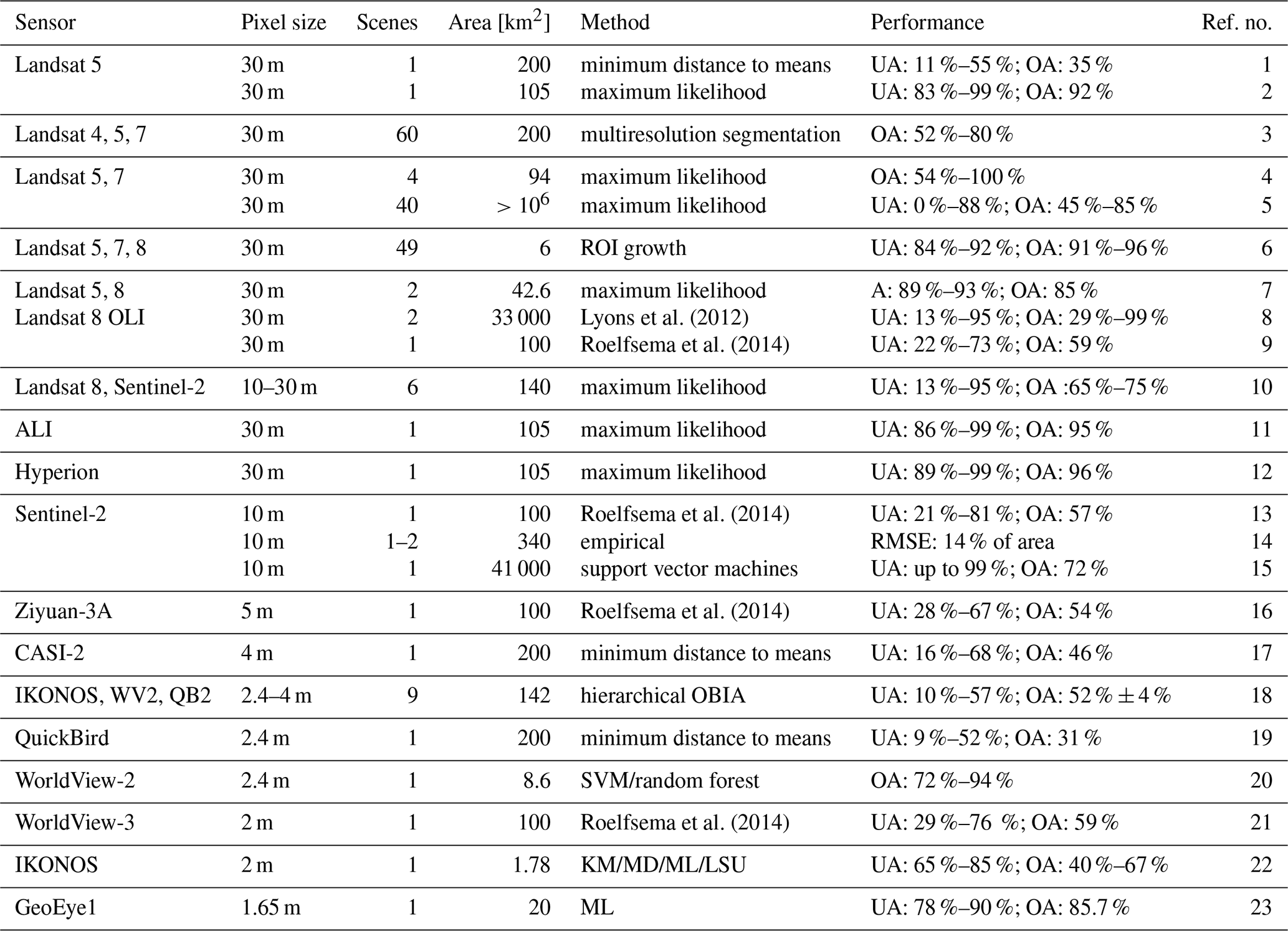
Lyons et al. (2012)Roelfsema et al. (2014)Roelfsema et al. (2014)Roelfsema et al. (2014)Roelfsema et al. (2014)Table 1Compilation of published works on seagrass detection from satellite data. References for the sources are given in Table A1 as indicated by the numbering in the last column. ROI: return on investment. OBIA: object-based image analyses. SVM: support vector machine. KM: k means. MD: minimum distance. ML: maximum likelihood. LSU: linear spectral unmixing.
Multiple monitoring campaigns, at several different sites and using diverse methods, have been conducted over the years to map seagrass cover, leading to the recent compilation of a global seagrass distribution assessment (McKenzie et al., 2020). Field mapping is widely employed to determine vegetation characteristics such as stem density, biomass, and metabolism (e.g. Smith et al., 1988; Caffrey and Kemp, 1991; Kutser et al., 2007), but high costs and long completion times prevent frequent surveys of the state and extent of submerged vegetation. And yet timeliness is particularly important in understanding the response of seagrass meadows to environmental stressors. In favourable conditions and in the growing season, seagrass can recover from heat waves (Pedersen et al., 2016; Gamain et al., 2018) or shallow scouring within just a few months (Collier and Waycott, 2014), making the effect of such disturbances invisible to infrequent observations. Remote sensing using multi- and hyper-spectral sensors constitutes an attractive alternative and complements field mapping, provided that detection methods can reliably classify the seabed. Such methods have been applied successfully to satellite data for salt marsh vegetation in the Venice Lagoon (Wang et al., 2007; Yang et al., 2020) as well as for the quantification of suspended sediment concentration (Volpe et al., 2011; Zhou et al., 2017); detecting seagrass using the same data sources remains challenging, due to highly variable water depth and constituents, but would allow for consistent environmental monitoring. Satellite-borne sensors also provide up to daily observations and are cost-efficient, making them an ideal support for high-frequency and spatially extended monitoring.
Table 1 reviews 16 publications concerning seagrass mapping from satellite imagery, ordered by decreasing pixel footprints of the image product. These studies classify seagrass density in steps of 25 % pixel surface cover, using various methods such as the maximum likelihood method (Cam, 1990), trained support vector machines (Noble, 2006), and random forest (Biau and Scornet, 2016) methods. Landsat data, with 30 m pixels that can be larger than some seagrass patches and few spectral bands, do not perform significantly worse than commercially available data with higher resolution and a larger number of bands, such as IKONOS. The wider range of performances for Landsat over other products may be a result of the greater number of studies that use this support. Overall, trained machine learning methods perform marginally better than more traditional classifiers on remote-sensing data of the same resolution. However, a systematic comparison among different classifiers can hardly be inferred from the literature because of the widely different resolutions explored in the existing studies. Indeed, the maximum likelihood classifier is used primarily on Landsat products. The wide variety of performances shown in such applications suggests a strong dependence of classification results on the quality of the data and the conditions in which the data were acquired. Indeed, atmospheric conditions, water depth, the presence of waves, and chlorophyll and sediment concentrations all affect reflectance at the water surface and thus the visibility of the seabed. As a result, acquisitions to be classified must be subject to a strict selection process, making frequent and regular monitoring difficult.
An inconsistent classification performance and the consequent irregular monitoring frequency (e.g. see Table 1) pose significant limitations to seagrass cover monitoring: the high primary productivity of seagrass implies that meadow density and canopy characteristics, and therefore spectral reflectance, vary greatly seasonally with growth stages and stochastically with storm-induced thinning or scouring (Sfriso and Francesco Ghetti, 1998). This high rate of variation in density and extent also implies that seagrass maps separated by more than a few months cannot capture seasonal, and much less stochastic, variations in seagrass cover. Yet few of the studies listed in Table 1 classify more than one image (Lyons et al., 2012; Dekker et al., 2005; Wabnitz et al., 2008; Hossain et al., 2015; Kohlus et al., 2020; Roelfsema et al., 2014), while most limit the analyses to single illustrative data acquisitions.
The observations made from Table 1 highlight the conclusions drawn by the extensive review of Hossain et al. (2014) in that while seagrass detection through remote sensing is imperfect, applications such as machine learning are used on extended time series of multispectral satellite images. For instance, Landsat products show the potential to improve greatly with more advanced processing, amongst which are the integration of ecological data or models. Here we apply a random forest (RF) classifier (Bakirman and Gumusay, 2020) to map seagrass cover in approximately 150 Landsat scenes between 1999 and 2020 from the Venice Lagoon, Italy. Based on nine field surveys performed between 2002 and 2017 as well as remote digitisations on images between 2000 and 2019, we investigate the influence of environmental conditions, known seagrass coordinates, and the temporal persistence of detected features on the performance of the classifier. By adding these features and corrections in the classification process, we take a step towards the integration of ecological data in classification models.
With a surface area of 550 km2, the Venice Lagoon is the largest lagoon in the Mediterranean Sea. Due to its socio-economic and environmental importance and to a significant erosional trend (Carniello et al., 2009), the ecological and morphological state of the lagoon has been systematically monitored for decades. Historic and modern bathymetric information complemented by a long record of tidal data provides the opportunity of quantitatively describing, also via numerical modelling, the detailed hydrodynamic circulation throughout the lagoon (Tommasini et al., 2019). Numerous sampling campaigns of sediment composition on the lagoon bed (Amos et al., 2004; Guerzoni and Tagliapietra, 2006; Carniello et al., 2012) are used to infer the preferred habitat of seagrass meadows, and multiple submerged vegetation surveys conducted throughout the 21st century provide a reference for classification testing.
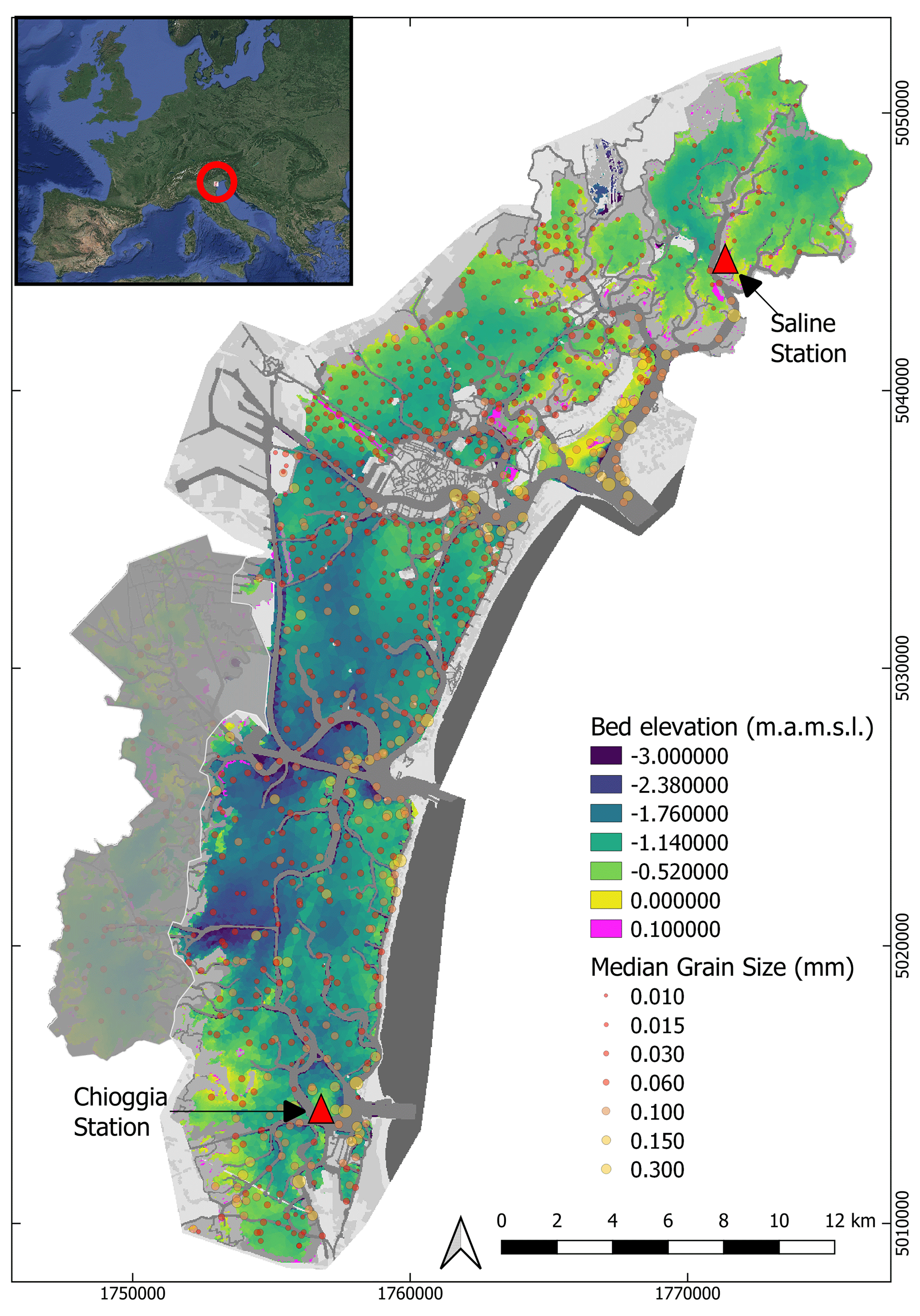
Figure 1Out-of-image data used as features for seagrass detection. Background image: gridded bathymetry of the Venice Lagoon, collected in 2003 and updated only for the inlets in 2012; data points: gridded median grain size. Triangles indicate the locations of tide and wind gauges. The grey area represents a zone in the lagoon where no seagrass was found during field surveys. The coordinate system used is the local Monte Mario projection (EPSG: 3003). Inset image: © Google Earth.
With this wealth of data, the Venice Lagoon is a prime candidate to test new approaches of submerged vegetation detection. In this section, we first describe the collection and processing of local data as well as satellite images from Landsat 7 ETM (Enhanced Thematic Mapper) and Landsat 8 OLI (Operational Land Imager) repositories, used as input and for validation. Then, we describe the structure of the random forest model developed to classify the images, and explain how local environmental data, as well as data pertaining to the coordinates of known seagrass patches, are added to improve the skill of the classifier. We also describe a simple process used to correct initial predictions, based on the analysis of the predicted seagrass cover time series. Finally, we define the metrics used to assess the classifier's performance.
2.1 Local data collection and processing
A full-lagoon bathymetric survey was performed in 2003 by the Venice Water Authority (Nuova-Technital, 2007) and subsequently updated to account for engineering works that modified the bathymetry within the inlets of Chioggia, Malamocco, and Lido (Carniello et al., 2009) (Fig. 1). Furthermore, samples of bed sediment composition have been collected over the years, resulting in a dataset of more than 900 estimates of median grain size (D50) (Carniello et al., 2012) (Fig. 1). A network of tidal and wind speed gauges has recorded hourly water surface elevation, wind speed, and direction in key locations of the lagoon since before 2000: among these, we chose stations close to Chioggia in the south and the Saline station in the north (red triangles in Fig. 1; source data: (https://www.comune.venezia.it/content/dati-dalle-stazioni-rilevamento, last access: 1 June 2021). Those stations were chosen as they have the most consistent record over the 1999–2020 period. The station in Saline records both wind velocities and tidal elevation, whereas these data are recorded by two separate stations, located 500 m apart, in Chioggia.
In addition to physical data, we used field surveys detailing the extent of seagrass cover, species composition, and stem density, hosted on the Atlante della Laguna website (http://cigno.atlantedellalaguna.it/maps/6/view last access: 1 June 2021).
These surveys were performed by SELC (https://www.selc.it/, last access: 1 June 2021) by delineating seagrass cover, both using a GNSS in the field and by having an operator digitise patches of seagrass from aerial images. Species identified during those surveys were principally Zostera noltii and Cymodocea nodosa, with Zostera marina and Ruppia maritima being found locally. The surveys were conducted and the images acquired to cover the entire lagoon in the late summer of 2002, 2004, 2009, 2010. and 2017.
However, given the extent of the lagoon, field surveys took place over periods of several months, such that they do not represent the state of the lagoon at a single moment in time. Furthermore, the criteria used to estimate seagrass cover may have varied over time or as a result of different observers. Additional surveys were conducted in the late summer of every year between 2006 and 2015, focusing on the inlets of Lido, Malamocco, and Chioggia (footprints appear in Fig. A1), mapping seagrass cover according to density classes derived from field, satellite, and aerial image observations. In this study, we do not use these density classes and instead regard all density classes that are not bare as vegetated. Indeed, this classification was likely performed by different operators over the years and introduces a source of uncertainty in reference maps. Finally, an operator digitised seagrass patches from 25 Landsat images between 2000 and 2020 on a specific tidal flat near Chioggia with a wide range of bathymetry, where visual inspection revealed multiple changes in seagrass cover (Fig. A1). This digitisation, conducted by visually distinguishing bare and vegetated areas, complemented existing reference maps to produce more frequent references and enable comparisons of vegetated surface area.
2.2 Satellite data collection and processing
We downloaded 164 cloud-free Level 2 multispectral acquisitions from the Landsat 7 ETM and Landsat 8 OLI data repository, covering the entire Venice Lagoon between 1999 and 2020. Landsat 5 data were not considered due to inconsistent results in the studies examined in Table 1. Level 2 products are atmospherically corrected using the LEDAPS (Schmidt et al., 2013) and LaSRC algorithms (Ilori et al., 2019) and yield surface reflectance values corrected for the scattering and absorbing effects of gas, vapour, and aerosols. In May 2003, the Scan Line Correction (SLC) system on the Landsat 7 ETM sensor failed, causing all subsequent ETM scenes to contain strips of empty data. Nevertheless, we did not disregard these acquisitions and take this into account when interpreting our results. From July 2013 onward, Landsat 8 OLI data were brought online, effectively resolving the issue for the purposes of our study. We selected a number of images among those downloaded according to two criteria (Fig. 2). (a) The tidal elevation at the full hour closest to overpass time is less than 0.75 m above the national datum (Rete Altimetrica dello Stato 1897). This value was chosen to cut off specific stormy events during which sediment load increased water column absorption and masked the lagoon bed; this approach was not complemented by the implementation of a correction for sediment suspended load to emulate situations where such models cannot be calibrated. (b) The third quartile of the series of wind speeds up to 3 d prior to overpass time does not exceed 8 m s−1 and the 90th percentile does not exceed 15 m s−1. This criterion limits the probability of inorganic suspended sediment and wind waves impacting visibility of the seabed. Applying these criteria leaves 148 scenes that are a priori fit for the detection of seagrass meadows on the lagoon bed.
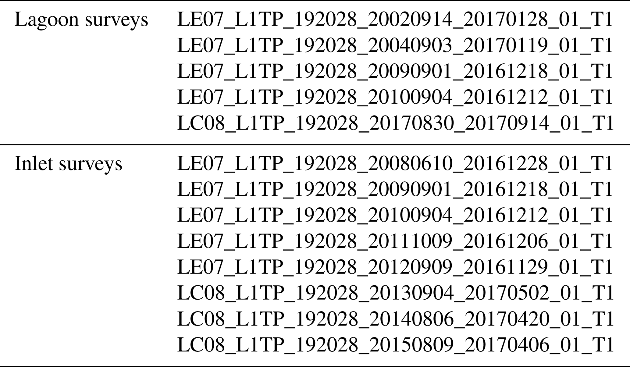
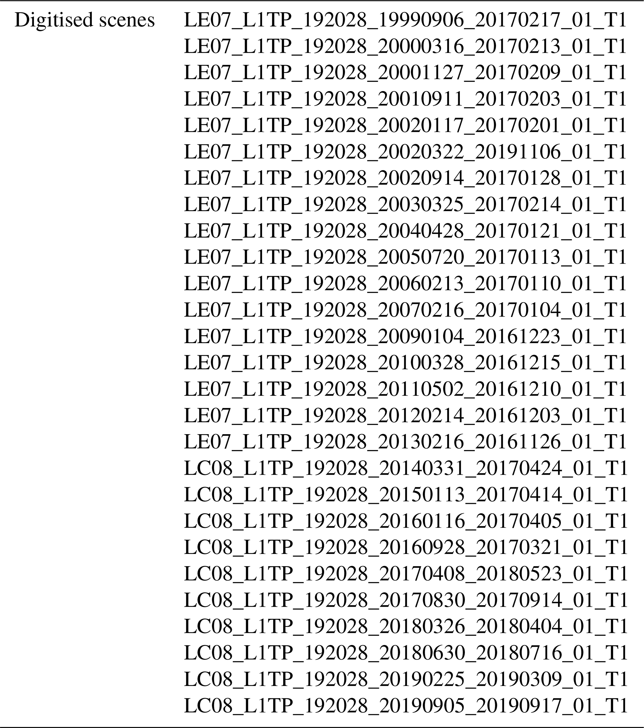
Landsat scenes corresponding to field surveys are listed in Table A2, while those associated with digitised reference information are shown in Table A3.
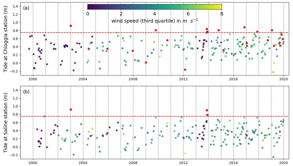
Figure 2Tide and wind conditions used to select Landsat scenes at the stations of (a) Chioggia and (b) Saline. The red dashed line shows the high limit for tidal elevation relative to station datum: scenes where water level exceeds this elevation were not selected and are shown in red. Scenes where wind speed exceeded the limit condition are also shown in red.
Bathymetric (Carniello et al., 2009) and sediment grain size data (Carniello et al., 2012), excluding channels and salt marshes, were gridded with the Geospatial Data Abstraction Library (GDAL) (GDAL/OGR contributors, 2021) at a pixel size of 30 m according to the nearest-neighbour method. All surveyed and digitised seagrass meadows, initially in vector format, were also rasterised using GDAL at a pixel size of 30 m, to match bathymetry and sediment size data. Seagrass cover vector data were gridded by regarding pixels covered by a seagrass polygon by more than 50 % as vegetated (coded as “1”). The remaining pixels were considered bare soil (coded as “0”).
2.3 Description of the random forest model
We used a random forest (RF) classifier designed to detect the presence of seagrass meadows on the lagoon bed based both on spectral and non-spectral information. Random forest modelling is an ensemble learning algorithm that uses the results of a large number of decision trees (Ho, 1995). This class of algorithms is being used more frequently in remote-sensing classification problems in general (Pal, 2005; Belgiu and Drăgu, 2016) and in seagrass detection in particular (Table 1). RF classifiers are trained to predict a set of target properties based on the values of a set of several features. Here, we train multiple classifiers to predict the absence (0) or presence (1) of seagrass in a given pixel, each with a different set of features and using different training target values.
Common features used to determine seagrass cover are the atmospherically corrected spectral reflectance values in the blue, red, green, and sometimes near-infrared bands (see references in Table 1). When the seagrass is submerged, these reflectances at the water surface are not linearly connected to the reflectance of the bed. Indeed, water depth, organic and inorganic suspended sediment concentrations, and water surface roughness, all contribute to define a complex relation between intrinsic seagrass reflectance and remote-sensing at-water-surface reflectance. These parameters are rarely simultaneously measured or acquired to be used in a radiative transfer model (Lee et al., 1998; Lee and Carder, 2002) to infer the bed reflectance. In this contribution, we retrieve red, green, blue, and near-infrared band data from selected Landsat and Sentinel images without applying a water column correction: instead, we test how the random forest performs under unknown water column influence, simulating conditions where calibration of inversion methods is problematic. We further note that the band width for the NIR band is different for Landsat and Sentinel images: consequently, when interpreting the model's performance on test data, we separate the performance of the model on images sourced from Landsat or Sentinel images.
Given the uncertainties affecting the spectral reflectance properties that may be retrieved from remote sensing, it is reasonable to leverage all available information with the aim to reliably perform seagrass mapping across multiple acquisitions.
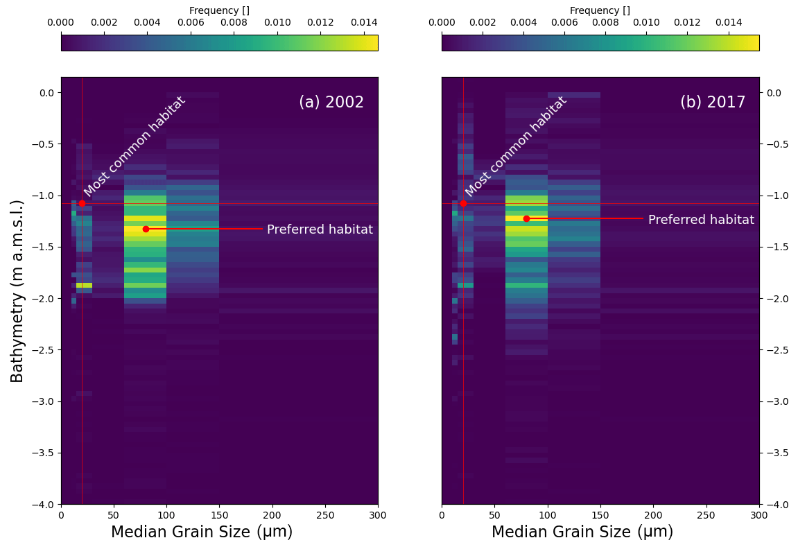
Figure 3Two-dimensional frequency distribution of seagrass according to bathymetry relative to IGM (Istituto Geografico Melitare)) reference and median sediment grain size (D50). (a) Seagrass distribution for the 2002 survey; (b) seagrass distribution for the 2017 survey.
Figure 3 shows the frequency distribution of seagrass meadows across bathymetry and median sediment grain size (D50) for full-lagoon field surveys performed in 2002 (Fig. 3a) and 2017 (Fig. 3b). We notice that seagrass meadows in the Venice Lagoon occupy a quite characteristic range of bed elevations, mostly between −2.1 and −0.5 m above datum and much narrower than the overall bathymetric range. Furthermore, the peak seagrass occurrence frequency does not correspond to the mode of the bathymetry (horizontal red lines); i.e. it is not located at the most commonly occurring bottom depth. This indicates that seagrass occurs within a preferential range of water depths, dictated by its need for access to light and by preferred flooding frequencies (Carruthers et al., 2002). Even more evidently, seagrass is preferentially found on fine sandy seabeds, where D50 ranges between 60 and 150 µm, even though these are not the most common sediment sizes in the lagoon (visualised by vertical red lines). Whether such ranges of bathymetry and sediment size are purely the expression of preferred habitat or the product of self-organisation and eco-geomorphic feedbacks is not debated in this contribution. However, the existence of a relationship between environmental parameters, such as bathymetry and D50 and seagrass distribution may be of assistance to developing effective algorithms for the detection of seagrass meadows.
A habitat constraint invariably translates into a constraint in geographical distribution. Figure 4 shows the geographical distribution of seagrass meadows across available field surveys described above, where each pixel expresses the cross-product ΠN in Eq. (1):
where N is the number of surveys considered and Vi is the array representing seagrass cover, with values comprising between 0 and 1. In both the full-lagoon and the inlet surveys, large swathes of seagrass meadows harbour Π=1 or Π=0 (shown as empty data in Fig. 4).
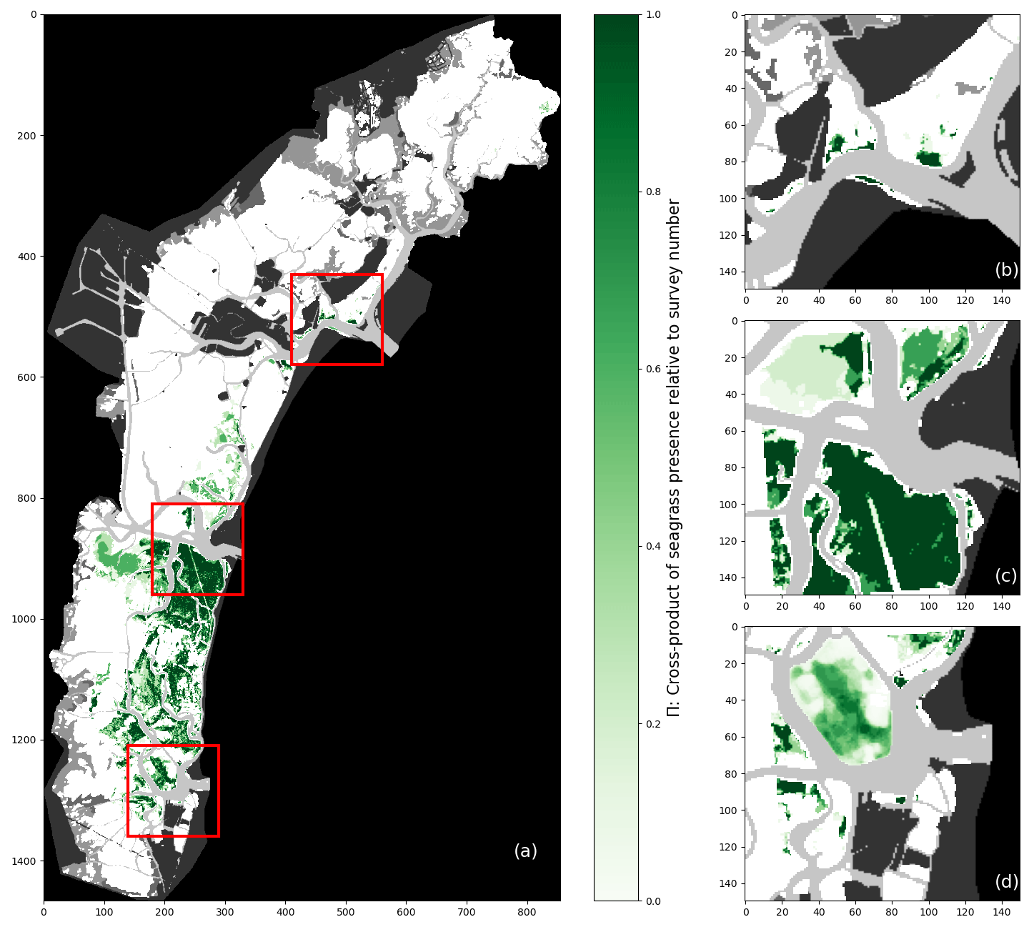
Figure 4Map of Π calculated for (a) five full-lagoon surveys and (b–d) six inlet surveys at the inlets of Lido (b), Malamocco (c), and Chioggia (d). Additionally, the area appearing blurred in (d) represents the map of Π for all surveys plus 25 manually classified images.
Figure 4 corroborates the notion that preferred habitats, shown simply in Fig. 3, constrain the geographical range of seagrass meadows in the Venice Lagoon. The north and central parts of the lagoon host patchy, disconnected meadows, while the southern lagoon hosts large interconnected meadows separated by navigation channels. This observation implies a degree of spatial auto-correlation in the presence of seagrass meadows, which may be explained by mechanisms of seagrass patch development: these are in general driven by environmental factors, such as differences in depth, nutrient fluxes, and salinity (Ghezzo et al., 2011; Sfriso et al., 2003), while clonal reproduction is the primary mechanism through which seagrass plants become established after an initial colonisation (McMahon et al., 2014) and sexual reproduction allow their spread over large distances.
The global Moran index provides additional evidence of spatial auto-correlation in seagrass distributions. This index represents the degree of spatial auto-correlation (SAC) for a dataset, varying between −1 and 1, with −1 corresponding to evenly spaced patches, 0 being the value approached by a random distribution of elements, and 1 being attained if a space is divided into two halves of contiguous elements of the same value (Fan and Myint, 2014). This further indicates a strong positive auto-correlation that suggests a zonation of the lagoon into areas, with some being favourable to seagrass development and others not. Here, all full-lagoon surveys present a global Moran index greater than 0.8. As a result, the value of pixel coordinates, expressed as row and columns in the array, may represent a useful feature in seagrass detection. Because such a feature carries the risk of introducing confirmation bias in the results, its influence on prediction variability will be examined closely.
Figures 3 and 4 show that features other than spectral reflectance have the potential to improve the performance of a classifier seeking to determine seagrass presence. To assess the impact of their inclusion among predictors on classification uncertainty, we train RF classifiers with a combination of features comprising spectral, environmental, and location-based features, as shown in Fig. 5. In order to be used simultaneously in the RF classifier, all features used were first normalised relative to the 5th and 95th percentile of their value in their respective zone (instead of the minimum and maximum). Because seagrass patches in the north and central parts of the lagoon show different sizes and density than in the southern lagoon, we divided the lagoon into two geographic zones at the Malamocco Inlet channel (see Fig. 4) and adopted a different RF classifier in each zone. The predictors (features) used are spectral reflectances, bed elevation, and D50. The RF classifiers, implemented in the scikit-learn package (Pedregosa et al., 2011), include 100 trees, each considering three input features with a maximum depth of 30 nodes. This RF classifier structure was chosen to avoid overfitting, which would limit the model's capacity to classify seagrass in the presence of a variable spectral response (caused by the presence of algae, local chlorophyll hotspots, etc.). The RF classifiers are trained using Landsat scenes taken on 14 September 2002 and 30 August 2017, with a training validation test ratio of , corresponding to field surveys conducted in the summers of 2002 and 2017. The ratio of bare vegetated pixels in the 2002 survey is in the north-central lagoon and in the southern lagoon; for the 2017 survey, it is and , respectively. Hence, the 2002 survey provides a balanced training dataset in the southern lagoon; other surveys and zones are imbalanced in favour of bare ground in the north and central parts of the lagoon and in favour of vegetation in the southern lagoon in 2017. In the discussion of our results, we examine how this imbalance may affect model predictions.
These survey dates were chosen over the remaining ones because the corresponding remote-sensing acquisitions are not affected by the Landsat 7 Scan Line Correction (SLC) failure. For each survey, we train one model per each northern/southern geographical zone and per each combination of features, resulting in eight RF models being trained in total. We then use these models to predict seagrass cover in 148 selected Landsat images (see Fig. 2).
2.4 Time-based correction
Seagrass cover predictions are liable to instability due to variations in data quality, water absorption, and scattering properties. The failure of the Landsat 7 ETM scan line corrector on 31 May 2003 caused all subsequent Landsat 7 ETM data to contain no-data strips, the position of which varies between images. To account for this discrepancy in data, we gave any no-data pixel at a given classification date t the classification it had in its previous classification t−1 and the following classification t+1, provided these were identical. If not, the pixel remains as no-data. Further instability in the predictions may be caused by classifications switching from bare to vegetated (or inversely) for a single image, for instance because of changes in seagrass or seabed reflectance caused by the intermittent presence of macroalgae or fishing activities. For instance, a pixel may appear bare for a set of contiguous scenes and then be classified as vegetated for one scene only, to return to a bare classification thereafter. Given the frequency of the scenes acquired, we consider it unreasonable to assume that seagrass patches appear or disappear in isolated scenes. Indeed, we considered it unlikely for both a scouring event and subsequent full recovery to occur within less than 5 months, which corresponds to the largest gap between images. Instead, these abrupt changes in seagrass classifications may be caused by the apparition or disappearance of algal patches, which appear similar to seagrass in the visible and infrared bands but, lacking a rooted anchor to the seabed, are more mobile than seagrass. Consequently, we applied the following post-processing correction rule: any pixel being classified in a scene at time t differently from classifications in scenes t−2, t−1, t+1, and t+2 (provided these are identical), is given the opposite classification. Finally, given the resolution of Landsat images, isolated patches of less than 4 pixels in surface area, whether they be bare or vegetated, are switched to the dominant classification around them. These corrected sets of predictions represent another set of eight predictions to validate (see Fig. 5).
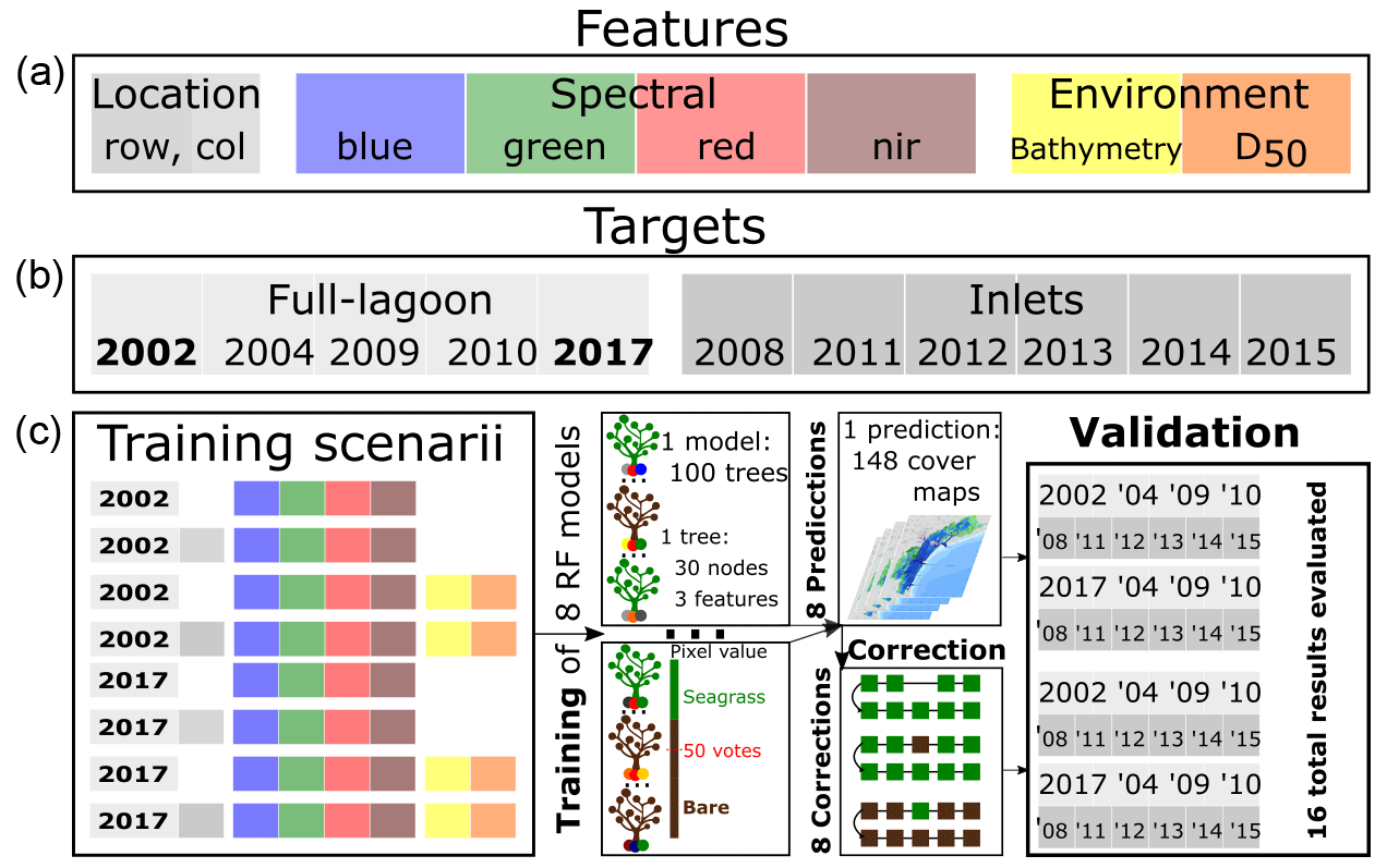
Figure 5Workflow of the study, depicting the different features used (a) and the target surveys and the year in which they were performed (b); in (c) the successive training, prediction, correction, and validation steps of the models are described.
2.5 Definition of model performance
For binary classifications such as the one performed here, model performance is quantified by the use of the numbers of true positives (TPs), true negatives (TNs), false positives (FPs), and false negative (FNs).
A global accuracy metric is defined as the ratio of true classifications (TP+TN) over the total number of pixels, a ratio often referred to as overall accuracy in non-binary classification problems (OA; see Table 1). In the Venice Lagoon, the presence of large areas of bare tidal flat relative to seagrass meadow area implies that OA is biased toward the correct prediction of bare tidal flats rather than toward the correct prediction of seagrass meadows (having a much smaller total area). Hence, sensitivity (S) (Eq. 2) and precision (P) (Eq. 3) give a measure of the model's performance that better fits our purpose, by eliminating TN:
S can be construed as a measure of the model's capacity to identify existing seagrass meadows. In non-binary problems such as those described in Table 1, S becomes the user's accuracy (UA) and is specific to each class. Conversely, P reflects the model's capacity not to include bare seafloor in the detected seagrass meadows and becomes the producer's accuracy (PA) in non-binary problems. These metrics may be combined through their harmonic mean F1 (Dice, 1945; Sorensen, 1948), defined in Eq. (4):
The F1 score increases non-linearly but symmetrically with S and P, allowing us to measure the model's performance through a single metric. Contrary to the OA accuracy, F1 does not include the term TN and is therefore not affected by the presence of extensive areas unequivocally classified as tidal flats: as such, this metric is more sensitive to changes in the detection of positives. The F1 score is used in the results section to describe the performance of the classifier, which we test on full-lagoon and inlet surveys as shown in Fig. 4.
3.1 Effect of added features
In this section, we describe the performance of the RF classifiers in all eight training scenarios before applying the time-based correction. Figure 6 shows this performance expressed as the F1 score.
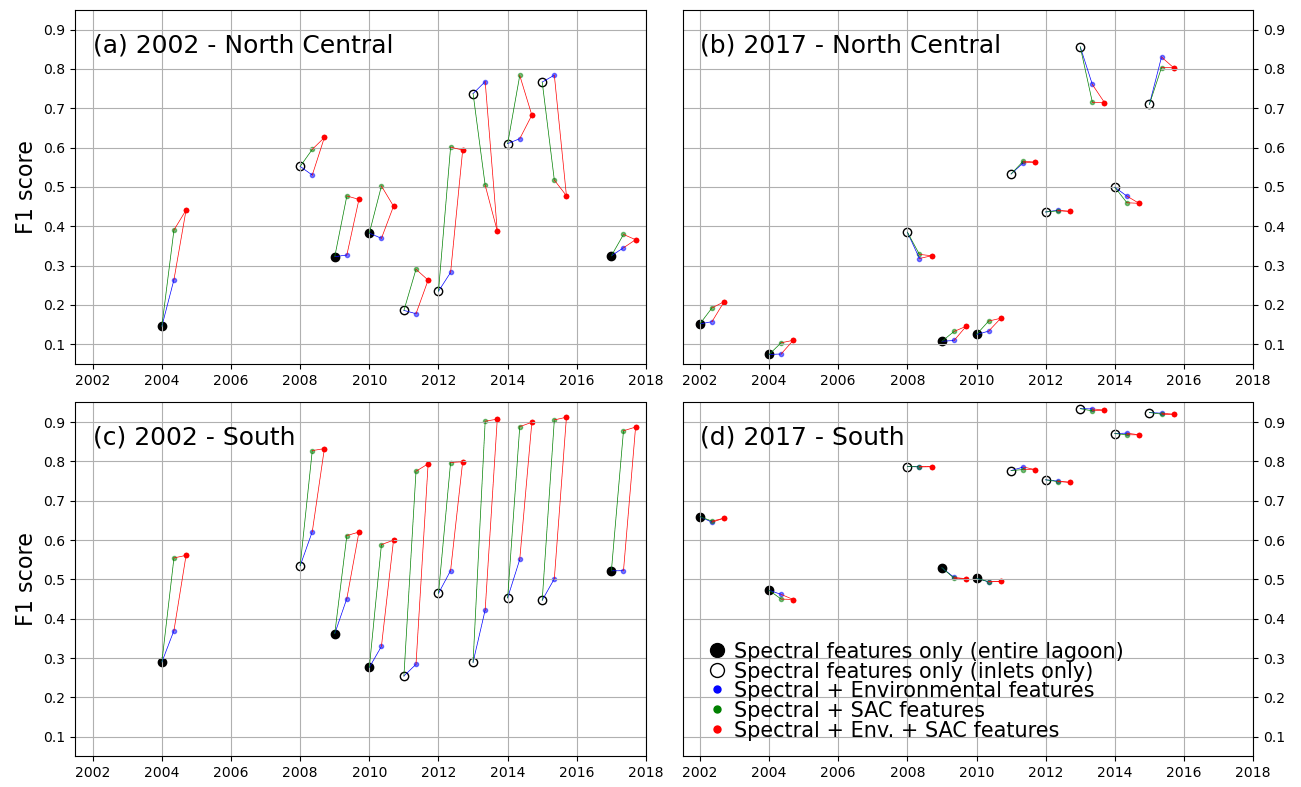
Figure 6F1 score of all models trained, tested on lagoon (full circles) and inlet (empty circles) surveys performed on the years indicated on the x axis. Black markers indicate models trained only with spectral features. The models tested were trained in the northern and central zone for the 2002 (a) and 2017 (b) surveys and in the southern zone for the 2002 (c) and 2017 (d) surveys.
Figure 6 highlights the different behaviours of models trained with the 2002 survey (a, c) with respect to those trained with the 2017 survey (b, d). We first examine the differences in performance between models using only spectral features, all trained on full-lagoon data and tested on either full-lagoon data (full circles) or inlet surveys (empty circles). Tests on full-lagoon data have generally lower F1 scores than tests on inlet surveys, particularly in 2017-trained models. This decreased performance on larger training datasets can be explained by slightly lower sensitivity values (Fig. A3) and significantly lower precision values (Fig. A2): this means that on test datasets including the full lagoon, models tended to more consistently classify bare ground as vegetated. This is a natural effect of testing on the full lagoon, where large areas, specifically in the north-central area, are bare and leave an opportunity for error in the prediction.
Models using only spectral features (black in Fig. 6) perform very differently than those including either environmental (blue, red) or spatial (green, red) features when trained on a 2002 survey. This is not the case if trained on the 2017 survey. Indeed, the addition of extra features to a 2002-trained model has a positive effect on the F1 score for most test instances (with exceptions in the north-central zone), with the addition of location features having the greater effect; in contrast it has a slightly negative influence on most 2017-trained models. Tests where full-lagoon surveys are less likely to over-identify vegetated areas (2002-trained models) are therefore more positively affected by the additional features. This indicates that the inclusion among the features of spatial position and environmental features produces large potential benefits, without generating significant negative effects on performance. Such advantages seem consistent as the same model formulation is tested across different images.
Decomposing this influence into the effects of sensitivity and precision (Figs. A2 and A3), we note that improvements occur mostly in the former, while the increase in precision is small (for 2002-trained models) or even negative (for 2017-trained models). In general, Figs. A2 and A3 show that 2002-trained models generally have higher precision but lower sensitivity values than 2017-trained models, indicating a tendency of the former to “miss” vegetated areas, while the latter will tend to overestimate the extent of seagrass meadows. In the southern zone, where most seagrass meadows are located, 2017-trained models using only spectral features perform significantly better than 2002-trained models. Models trained on 2017 data also perform consistently better when tested on inlet surveys rather than lagoon surveys, suggesting that false predictions lie outside the inlet areas. Conversely, 2002-trained models in the southern zone benefit the most from the addition of environment and coordinate features, improving F1 scores from under 0.5 to up to 0.9. Because the north-central zone harbours much less extensive seagrass than the southern zone, F1 scores are more difficult to evaluate in this region.
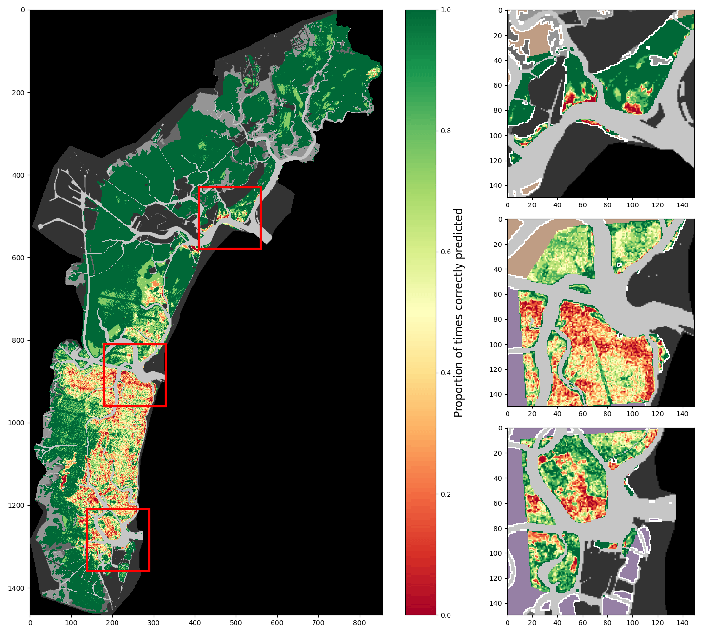
Figure 7Proportion of correct predictions of a 2002-trained model using spectral features only, tested on all surveys (lagoon, inlets, and digitised meadows).
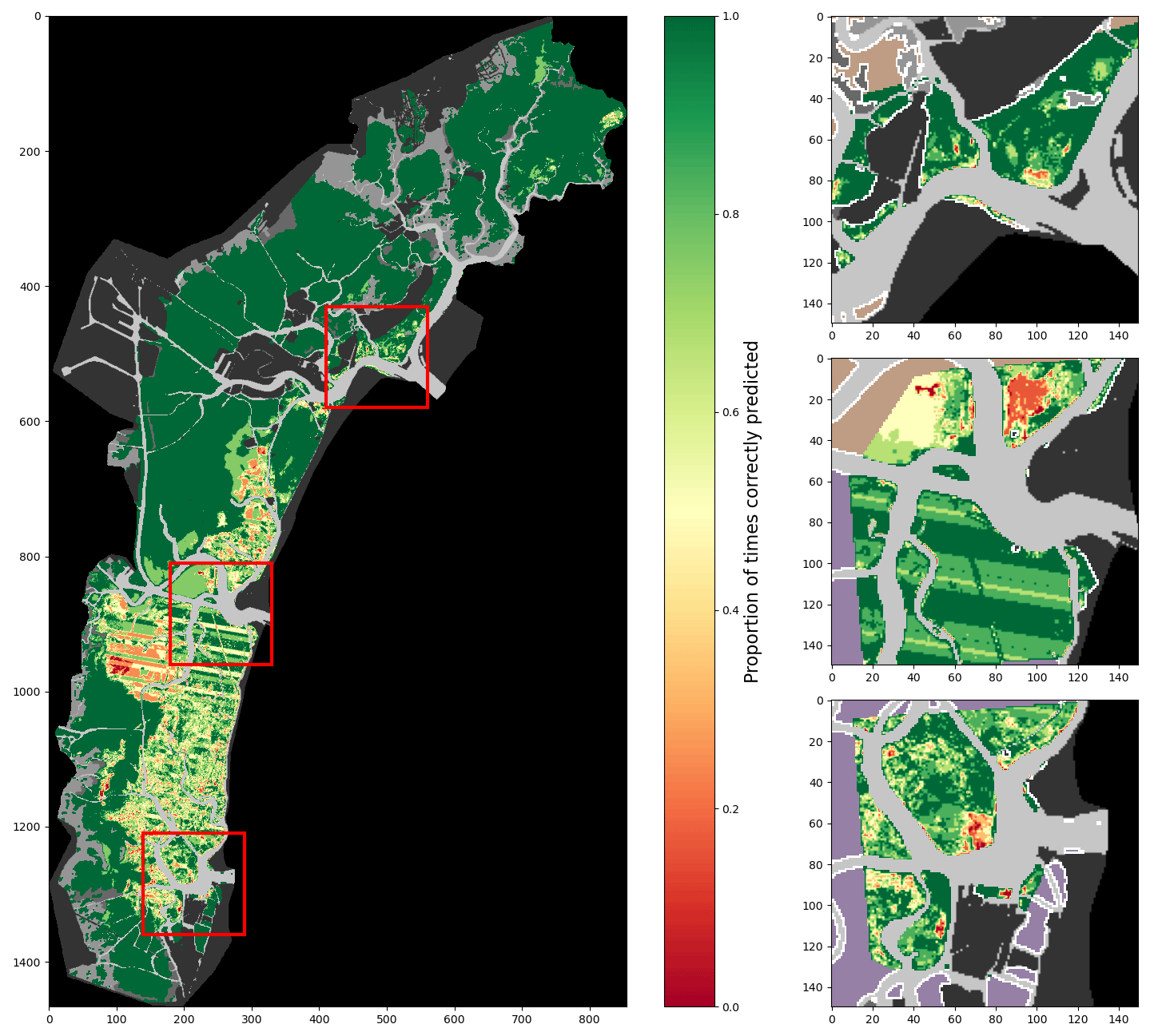
Figure 8Proportion of correct predictions of a 2002-trained model using all described features, tested on all surveys (lagoon, inlets, and digitised meadows).
Figures 7 and 8 demonstrate visually the effect of location features on model behaviour, providing an overview of the performances of a 2002-trained model on all other training data combined. Each figure maps, for each pixel of the full lagoon and in more detail for the three inlets, the proportion of test surveys for which a given pixel is correctly classified, whether bare or vegetated. Because not all pixels are associated with the same number of surveys, colour contrast is variable, with starker contrast appearing in areas where fewer surveys exist. Figure 7 shows the performance of a model using only spectral features, whereas Fig. 8 shows that of a model using both environmental and location features. The comparison of these two figures, with Fig. 4 as a reference, reveals several points of interest regarding the effect of the additional features on model performance. In both maps, some areas are consistently and correctly classified as bare: for example, in the north-westernmost area of the lagoon, correct prediction rates are equal to 1 over large surfaces. Such areas are spectrally unambiguous, with a relatively high seabed and light sediment which is never mistaken for seagrass by the model. Conversely, areas that are vegetated in at least one survey are rarely correctly classified as such in all tests (i.e. the proportion of correct predictions is below 1), particularly when using only spectral features: from this we deduce that seagrass, if confused by the model with bare ground, exhibits low separation between its spectral properties and that of bare ground in the bands used. This is particularly true in the southern lagoon, where the water column is generally thicker. Furthermore, when using only spectral features, maps of correct prediction rates appear “grainy”: this reflects irregularities in reflectance on the seabed or in seagrass patches – irregularities which cause local misclassifications. Irregularities are significantly reduced when adding environmental and location features. With fewer local misclassifications, models using these additional features generate more cohesive seagrass meadows: consequently, applying these models to monitor seagrass meadow evolution in time is less likely to erroneously predict changes inside the meadows, thus reducing errors in surface area change. The reduction in prediction “grain” also enhances, in Fig. 8, wide swathes of lower correct prediction rates: these swathes are an artefact of the ETM Scan Line Correction failure and are unclassified in some images. It is interesting to compare Figs. 7 and 8, obtained with a 2002-trained model with relatively well-balanced training data, to Figs. A4 and A5, which use less-balanced training data. In these figures, large areas are consistently misclassified regardless of features used, attesting to an inadequate training dataset. In such a case, the addition of features has very little effect on model performance, as previously shown in Fig. 6.
3.2 Effect of time-based correction
Figure 9 demonstrates the effect of the time-based correction process described in Sect. 2.4 on correct prediction rates, complementing Figs. 7 and 8. It showcases the increase in the rates of correct prediction at almost all points of the map brought by this correction, with the notable exception of areas for which correct prediction rates were already below 50 %. This is a direct consequence of the method of the time-based correction, which confirms classifications through time even if they are incorrect. Such an effect is unfavourable for models that perform poorly before correction, as showcased by Fig. A6, where large areas where correct predictions occurred in less than 50 % of tests dropped to 0. This further highlights the fact that models trained on imbalanced training data are ill-suited for the modifications proposed in this contribution. It also shows the elimination of swathes of lower rates through unclassified data, as it assumes continuity of classification between scenes.
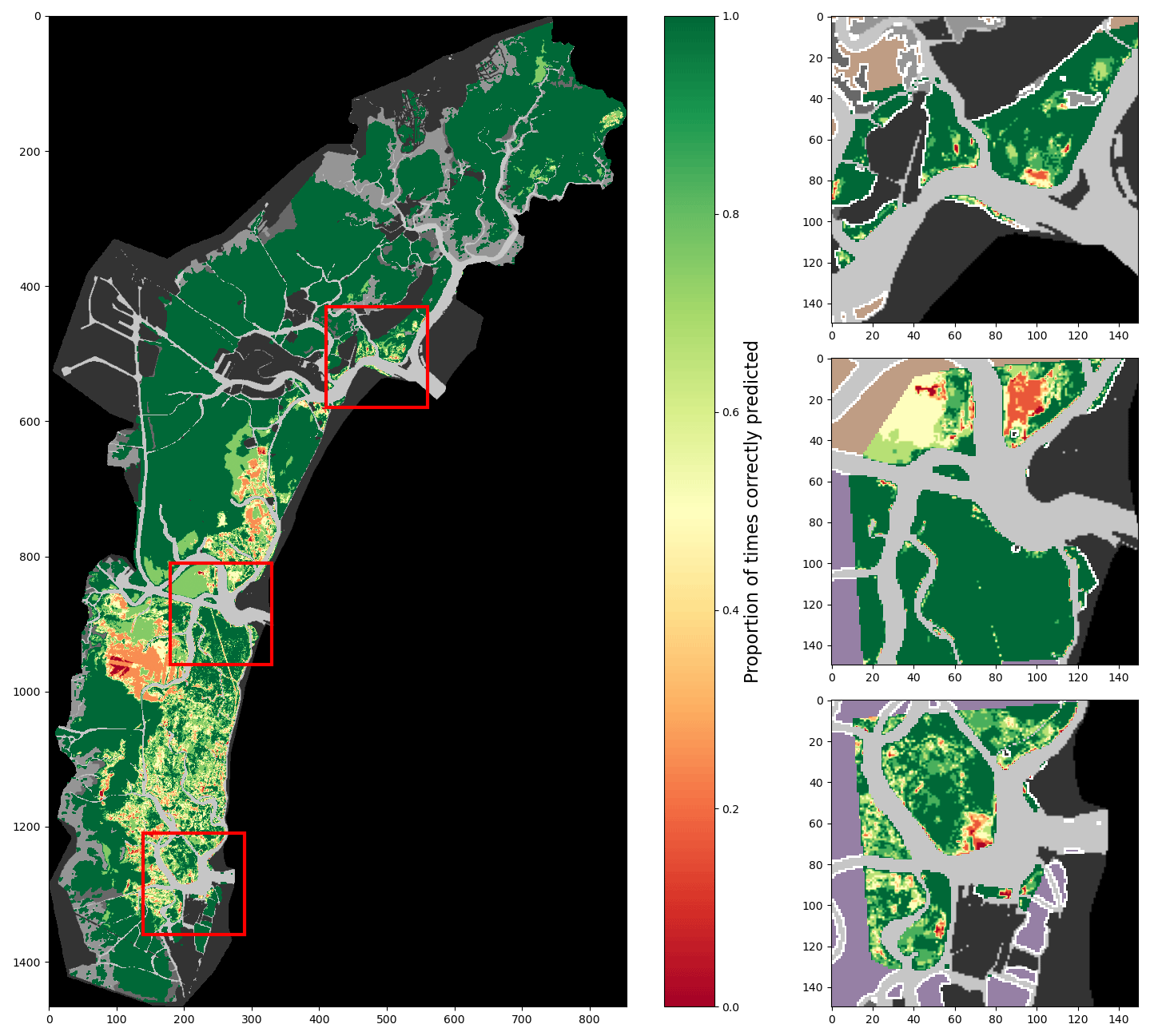
Figure 9Proportion of correct predictions of a 2002-trained model using all described features and after time-based correction, tested on all surveys (lagoon, inlets, and digitised meadows).
Figure 10 examines the effect of the time-based correction process described in Sect. 2.4 on the F1 score of all tested models.
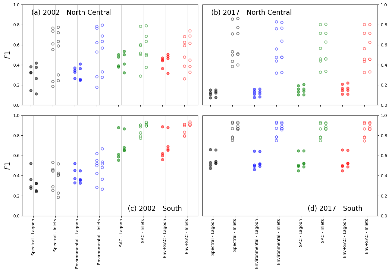
Figure 10Comparison of F1 scores before and after time-based correction (respectively, left and right of vertical bars), tested on lagoon (full circles) and inlet (empty circles) surveys. The models tested were trained in the north-central zone for the 2002 (a) and 2017 (b) surveys and in the southern zone for the 2002 (c) and 2017 (d) surveys.
In the north-central zone (a, b), no obvious pattern in the change in F1 after correction is detected. In the southern zone (c, d), however, both 2002-trained models and 2017-trained models respond in a discernible pattern to the application of the time-based correction: of the 2002-trained models (c), models using only spectral or spectral and environmental features, which have a lower F1 score initially, generally see a decrease in F1 after correction, whether they are tested on the full lagoon or at the inlets. This coincides with the lower F1 scores for these models' predictions. Conversely, models including known seagrass locations as features, for which predictions initially have a higher F1 score, mostly see an increase in F1 scores. For these models, it appears that the F1 score after time-based correction has a stronger positive effect the higher the initial F1 score. For 2017-trained models (d), the addition of features having little effect, the time-based correction has a uniform effect regardless of features . Notably, whether for lagoon or inlet surveys, tests conducted during the period of the Landsat 7 SLC failure display lower F1 values (see Fig. 6d) as well as the largest positive change in F score after correction: this suggests that the proportion of true positives reinstated through the time-based correction outweighs the proportion of false predictions added in the process.
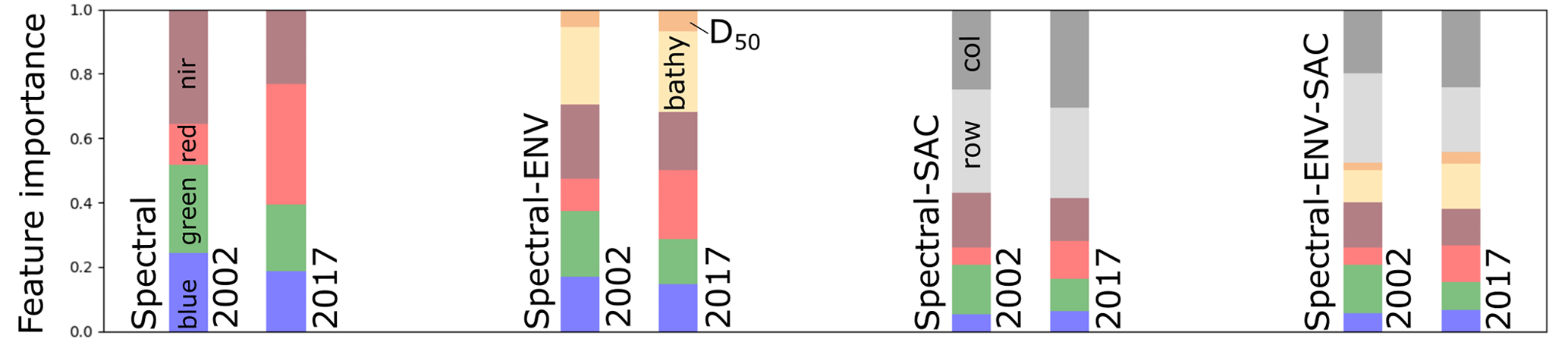
Figure 11Relative importance of each feature used in models trained with 2002 and 2017 data.
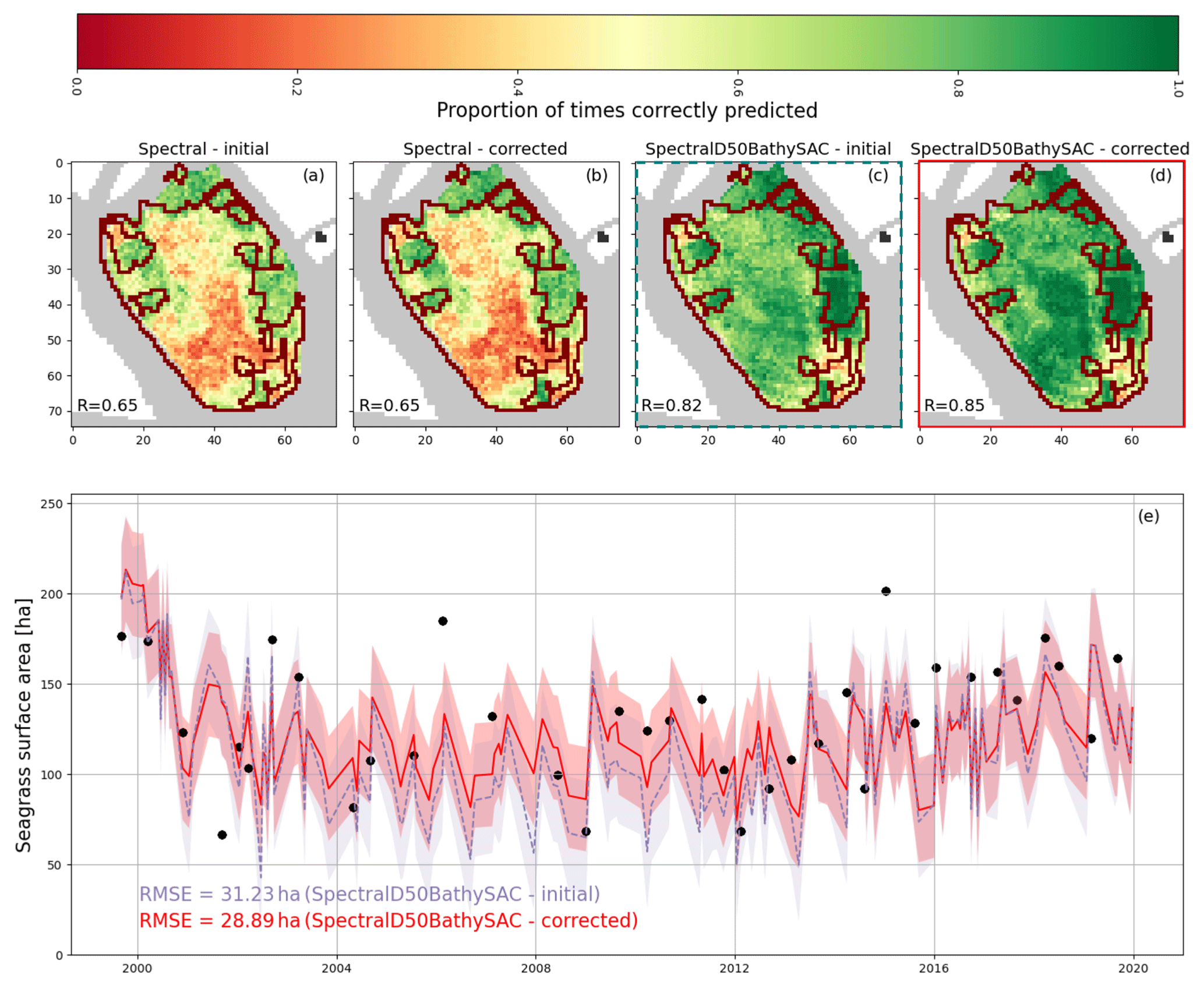
Figure 12(a–d) Map of the proportion of surveys correctly identified for 36 surveys and digitisations combined. R represents the average value across all mapped pixels. Red outlines show the extent of seagrass patches in the summer 2002 survey; (e) surface area of seagrass predicted by surveys framed in (c) and (d), filled with the RMSE value. Black dots indicate surveyed or digitised surface area value.
Several key issues pertaining to the reliability of seagrass detection arise from the examination of the performance of the models in Sect. 3: first, the strong disparity in performance, expressed through the F1 score between models trained using data from 2002 and 2017; then, the significant difference in the influence of environmental and, particularly, spatial features on F1 scores; finally, the opposing effects of time-based correction on the performance of different models. The behaviour of RF models being non-linear, we do not presume to identify a general relationship between the observations made in a single case study and the performance of seagrass cover predictions using an RF classifier. Nevertheless, we attempt to break down the influence of additional features and time-based corrections, using the southern zone, where most seagrass is found, as a testing ground. Figure 11 shows the relative importance of features employed in each RF classifier used, where location features dominate, when present, for both 2002-trained and 2017-trained models. In all scenarios, the red band is the most important spectral band for 2017-trained models. As this band is particularly sensitive to suspended sediment concentration, we may surmise that its high importance could impede classification performance, particularly if turbidity is not accounted for in the classification. Conversely, the near-infrared band shares the highest importance among spectral features with the green band. Given the sensitivity of the NIR band to suspended chlorophyll concentrations, the importance of this band may be conceived of as a potential hindrance to the performance of the RF. We note however that in previous iterations of the RF using only the RGB bands, performance was not only lower after adding positional and environmental features and time-based corrections but also before the applications of these modifications, despite the difference in band width between Landsat 7 and Landsat 8; This disparity may contribute to the diverging behaviours of the models trained on 2002 or 2017 data.
In Sect. 1, we mentioned the difficulty of producing consistent seagrass cover predictions at a high frequency. Figure 12 showcases the potential use of location and environmental features to improve the reliability of seagrass cover predictions, demonstrated on a 2002-trained model. Panels a–d are each a map of the success rate of seagrass cover predictions for each pixel near Chioggia Inlet, shown in yellow in Fig. A1, tested on 36 reference datasets from surveyed and digitised seagrass cover. In each panel, R represents the average success rate. In dark red, panels a–d show the outlines of vegetated patches in the summer 2002 survey. In panels a and b, where only spectral features were used, we observe that pixels with lower prediction success rates overlap with those with higher occurrence rates but not necessarily with the presence of seagrass in the summer 2002 survey. Panels c and d, both of which include location features as well as environmental features, experience a notable increase in prediction success rates in these regions. Notably, increases in success rate match areas of high Π value (see Fig. 4d), suggesting that where spectral features alone did not detect the presence of seagrass, models with all features did. Furthermore, we note that the implementation of the time-based correction shown has little effect on R when using only spectral features (b) but causes an increase when other features are used. This is consistent with our previous observation that the time-based correction mostly improves predictions of higher initial quality.
In panel e, we further note that seagrass surface area predictions decrease by up to a factor of 2 in the year 2000, suggesting that location features are not demonstrably impeding the model's capacity to predict seagrass surface area change. The root mean square error (RMSE) after implementing the time-based correction is 28.89 ha, a 7.5 % decrease in RMSE with respect to predictions without the time-based correction, and amounts to 22 % of the average seagrass surface area in the examined pixels. This value matches and exceeds half of the variation in seagrass surface area between most dates where vegetation cover is predicted. While the error in surface area prediction remains high for the purposes of monitoring high-frequency changes in seagrass cover, it represents a significant improvement over models using only spectral features and no time-based corrections.
While the error in surface area prediction remains high for the purposes of monitoring high-frequency changes in seagrass cover, the improvements made over models using only spectral features and without time-based corrections are significant. This result points to future research avenues in seagrass monitoring. First, performance increases achieved through incorporating coordinates as features validate the notion that observed seagrass meadows are a good proxy for favourable habitat. Second, performance improvements achieved through time-based corrections show that real-world dynamics that bound the growth and degradation of seagrass meadows positively influence remote-sensing results. Together, these observations indicate that remote-sensing methods would benefit from being coupled with habitat and ecological models. Ultimately, such coupled classification models may be able to detect the intra-and inter-annual variability observed in digitised seagrass cover: in large habitats such as the Venice Lagoon, these models would allow the identification of seagrass degradation events and quantify regrowth and colonisation at scales that are impractical to observe through fieldwork.
In this contribution, we implemented several random forest classifiers using various sets of features, supplemented by time-based corrections, to detect the spatial and temporal dynamics of seagrass meadows in the Venice Lagoon. We trained eight such models using a combination of spectral data, bathymetry, median sediment grain size, and coordinates of known seagrass extent as features. Four models were trained using data taken from field surveys and Landsat images of summer 2002 and four others with data taken in 2017.
We found that 2002-trained models and 2017-trained models responded differently to both the addition of out-of-image features and to the time-based correction. Adding location information was shown to significantly improve the F1 score without preventing the model from detecting variations in seagrass cover but only for 2002-trained models. Examining the importance of different features in each of the models, we observed that 2002-trained models and 2017-trained models were under the dominating influence of seagrass location when used but otherwise did not share the same most important spectral features. This may be a reason for their discordant behaviour. Furthermore, the vote count, which expresses the probability of a given pixel to be seagrass according to an RF model, was generally more polarised toward extreme values in 2017-trained models. While not a root cause of the difference between the sets of models, it revealed the effect of using geographic location features on tree voting. This shows that true change in seagrass meadows can be detected by location-dependent models when taking into account prior knowledge of seagrass location. Ultimately, accurately accounting for spatial auto-correlation will require the examination of more cases as well as a generally applicable formulation of its influence.
This contribution demonstrated the potential of mixing spatial auto-correlation patterns and time-series analysis with commonly used spatial detection methods, such as random forest classifiers to increase the performance of submerged vegetation detection methods. The positive effects of these modifications to standard methods have been shown to outweigh their potential “side effects”, although further research is required to generalise their influence. The resulting increased confidence in each seagrass cover map allows the generation of dense sequences of maps, through which the space–time dynamics of seagrass meadows may be described and connected to their governing environmental drivers. This, in turn, can inform ecological models and sediment transport simulations and ultimately feed into predictions of tidal basin response to environmental change.
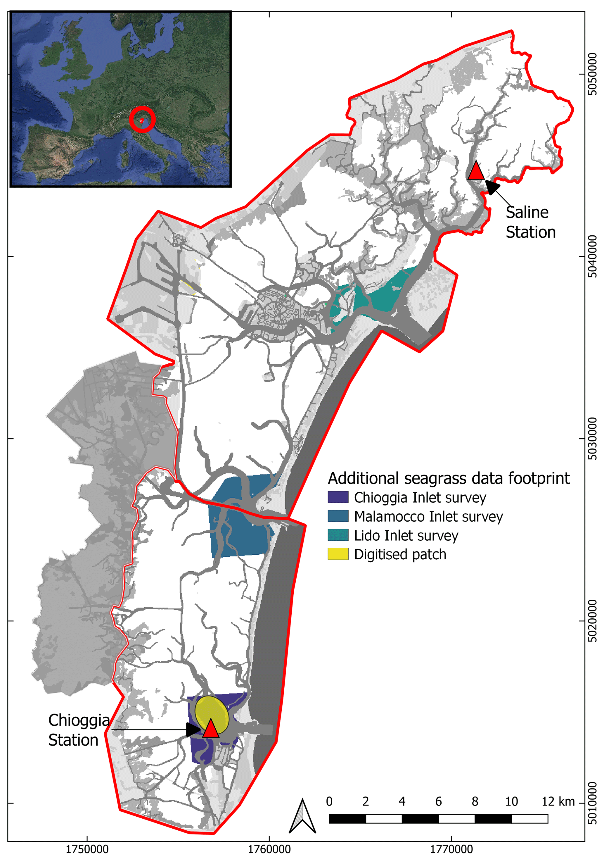
Figure A1Footprint of the inlet surveys of Lido, Malamocco, and Chioggia (blues) and of the digitised patch (yellow). The coordinate system used is EPSG: 3003. Inset image: © Google Earth.
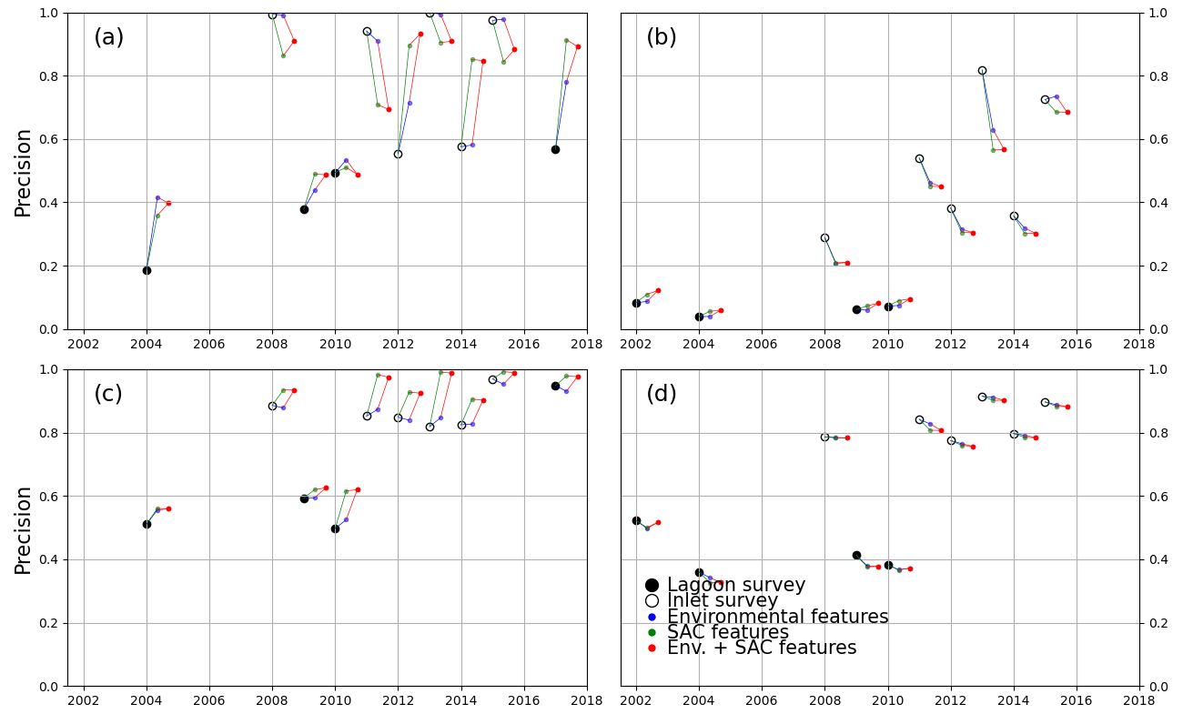
Figure A2Precision score of all models trained, tested on lagoon (full circles) and inlet (empty circles) surveys performed on the years indicated on the x axis. Black markers indicate models trained only with spectral features. The models tested were trained in the north-central zone for the 2002 (a) and 2017 (b) surveys and in the southern zone for the 2002 (c) and 2017 (d) surveys.
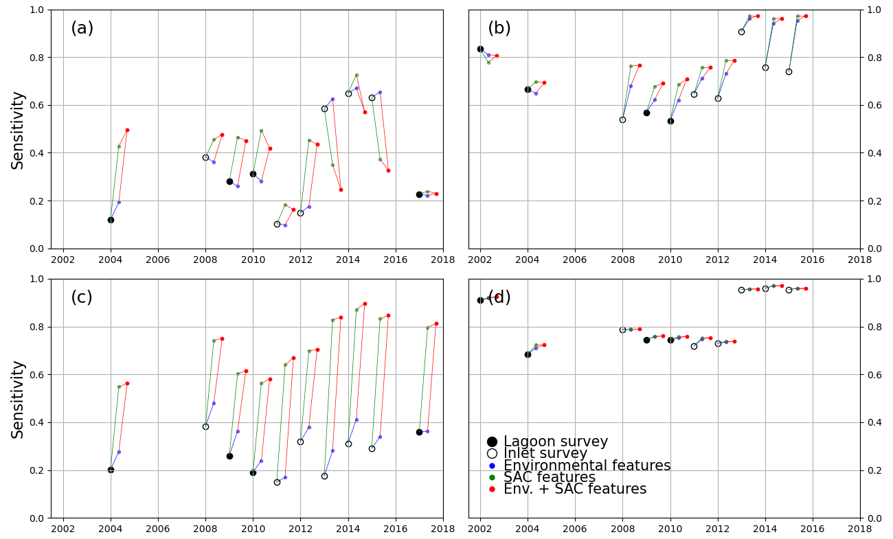
Figure A3Sensitivity score of all models trained, tested on lagoon (full circles) and inlet (empty circles) surveys performed on the years indicated on the x axis. Black markers indicate models trained only with spectral features. The models tested were trained in the north-central zone for the 2002 (a) and 2017 (b) surveys and in the southern zone for the 2002 (c) and 2017 (d) surveys.
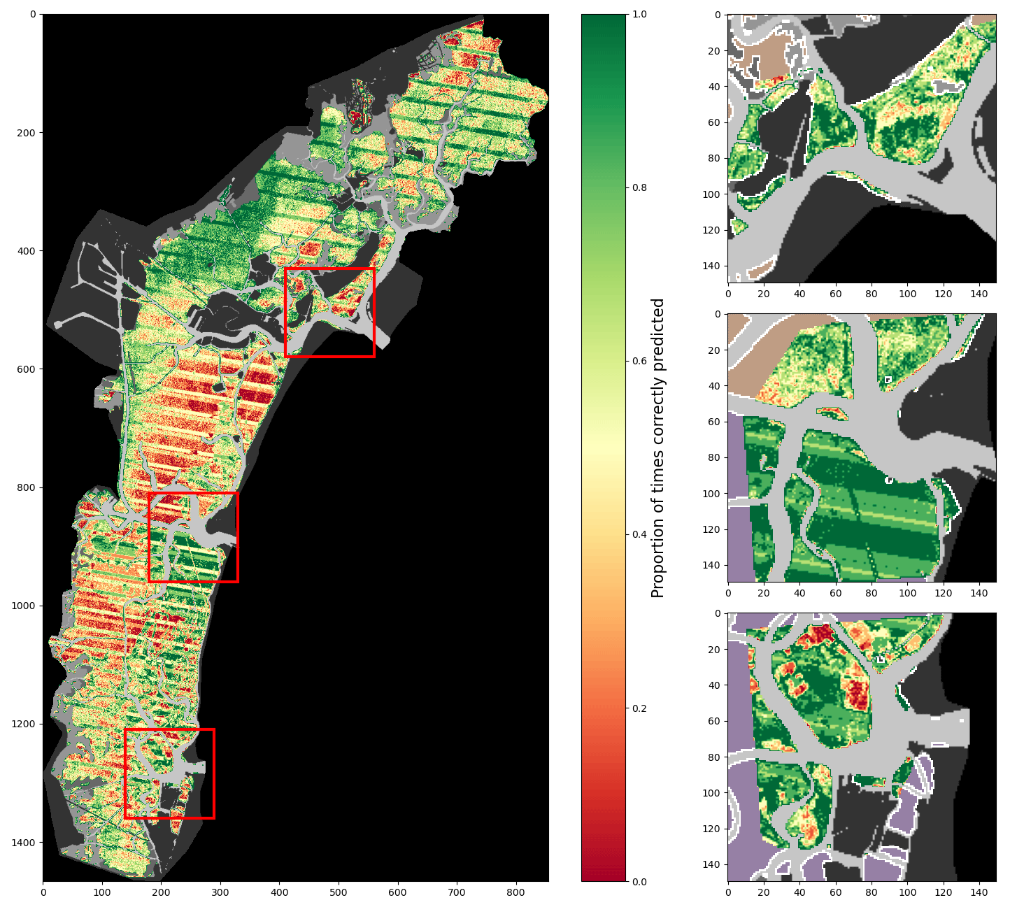
Figure A4Percentage of correct predictions of a 2017-trained model using only spectral features tested on all images (lagoon, inlets, and additional digitisations combined).
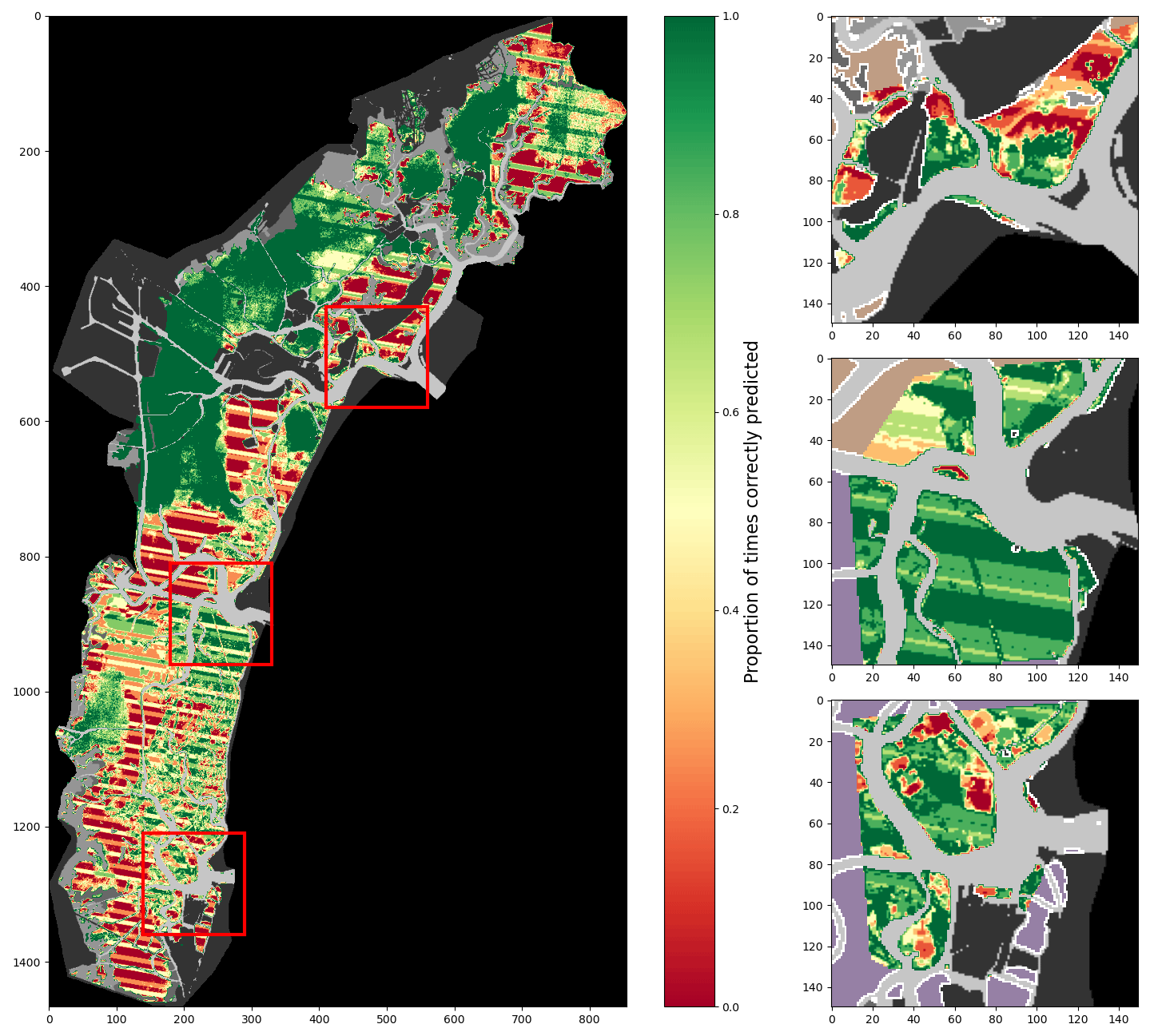
Figure A5Percentage of correct predictions of a 2017-trained model using all considered features tested on all images (lagoon, inlets, and additional digitisations combined).
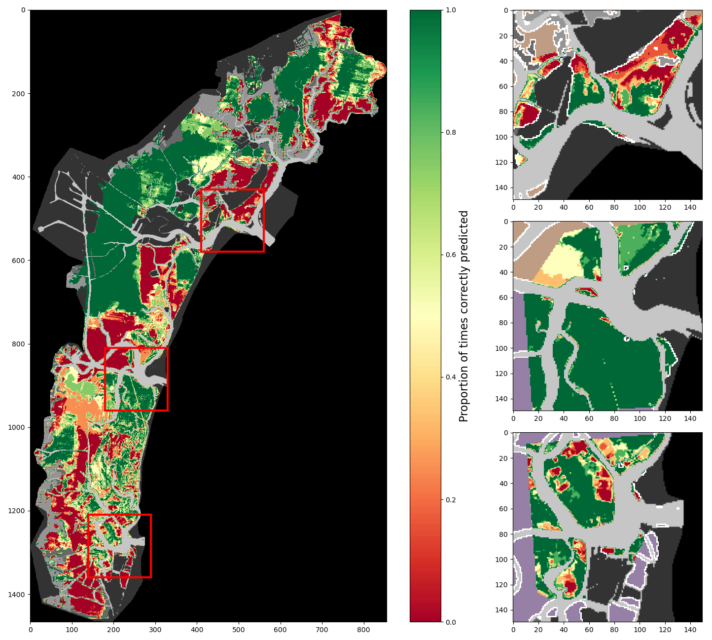
Figure A6Percentage of correct predictions of a 2017-trained model using all features and the time-based correction tested on all images (lagoon, inlets, and additional digitisations combined).
Table A1Compilation of published works on seagrass detection from satellite data.
Table A2Selected Landsat scenes with full-lagoon or inlet surveys.
The satellite data used in this contribution are openly available on multiple platforms, including NASA's EarthExplorer (https://earthexplorer.usgs.gov/, USGS, 2021). The data concerning seagrass cover surveys, bathymetry, and median sediment grain size are openly available via the Atlante della Laguna at Guerzoni and Tagliapietra (2006). Tide and wind gauge data are openly available at https://www.comune.venezia.it/content/dati-dalle-stazioni-rilevamento (Città di Venezia, 2021).
Conceptualisation: GG, LC, AD'A, MM, and SS. Methodology: GG, LC, AD'A, MM, and SS. Software: GG. Validation: GG, LC, AD'A, MM, and SS. Formal analysis: GG. Investigation: GG. Resources: MM. Data curation: GG. Writing (original draft preparation): GG. Writing (review and editing): GG, LC, AD'A, MM, and SS. Visualisation: GG. Supervision: LC, AD'A, MM, and SS. Project administration: MM. Funding acquisition: MM. All authors have read and agreed to the published version of the paper.
At least one of the (co-)authors is a guest member of the editorial board of Biogeosciences for the special issue “Monitoring coastal wetlands and the seashore with a multi-sensor approach”. The peer-review process was guided by an independent editor, and the authors also have no other competing interests to declare.
Publisher’s note: Copernicus Publications remains neutral with regard to jurisdictional claims in published maps and institutional affiliations.
This article is part of the special issue “Monitoring coastal wetlands and the seashore with a multi-sensor approach”. It is not associated with a conference.
This research was funded by CORILA under the project Venezia 2021 (grant CUP D51B02000050001).
This research has been supported by the scientific activity performed as part of the Venezia 2021 Research Programme, coordinated by CORILA, with the contribution of the Provveditorato for the Public Works of Veneto, Trentino Alto Adige, and Friuli Venezia Giulia, Research Line 3.2 (PI A.D.). The University of Padova SID2021 project, “Unraveling Carbon Sequestration Potential by Salt-Marsh Ecosystems”, is also acknowledged (PI A.D.). This study was funded within the RETURN Extended Partnership and received funding from the European Union NextGenerationEU (National Recovery and Resilience Plan – NRRP, Mission 4, Component 2, Investment 1.3 – D.D. 1243 2/8/2022, PE0000005).
This paper was edited by Manudeo Singh and reviewed by T. Bakirman and one anonymous referee.
Amos, C., Bergamasco, A., Umgiesser, G., Cappucci, S., CLoutier, D., DeNat, L., Flindt, M., Bonardi, M., and Cristante, S.: The stability of tidal flats in Venice Lagoon – the results of in-situ measurements using two benthic, annular flumes, J. Mar. Syst., 51, 211–241, https://doi.org/10.1002/esp.4599, 2004. a
Amran, M. A.: Mapping seagrass condition using google earth imagery, J. Eng. Sci. Technol. Rev., 10, 18–23, https://doi.org/10.25103/jestr.101.03, 2017. a
Bakirman, T. and Gumusay, M. U.: Assessment of machine learning methods for seagrass classification in the mediterranean, Balt. J. Modern Comput., 8, 315–326, https://doi.org/10.22364/BJMC.2020.8.2.07, 2020. a, b
Belgiu, M. and Drăgu, L.: Random forest in remote sensing: A review of applications and future directions, ISPRS J. Photogram. Remote Sens., 114, 24–31, https://doi.org/10.1016/j.isprsjprs.2016.01.011, 2016. 011 a
Biau, G. and Scornet, E.: A random forest guided tour, Test, 25, 197–227, https://doi.org/10.1007/s11749-016-0481-7, 2016. a
Caffrey, J. M. and Kemp, W. M.: Seasonal and spatial patterns of oxygen production, respiration and root-rhizome release in Potamogeton perfoliatus L. and Zostera marina L., Aquat. Bot., 40, 109–128, https://doi.org/10.1016/0304-3770(91)90090-R, 1991. a
Cam, L. L.: Maximum Likelihood: An Introduction, Int. Stat. Rev., 58, 153–171, https://doi.org/10.2307/1403464, 1990. a
Carniello, L., Defina, A., and D'Alpaos, L.: Morphological evolution of the Venice lagoon: Evidence from the past and trend for the future, J. Geophys. Res.-Earth, 114, 1–10, https://doi.org/10.1029/2008JF001157, 2009. a, b, c
Carniello, L., Defina, A., and D'Alpaos, A.: Modeling sand-mud transport induced by tidal currents and wind waves in shallow microtidal basins: Application to the Venice Lagoon (Italy), Estuar. Coast. Shelf Sci., 105–115, https://doi.org/10.1016/j.ecss.2012.03.016, 2012. a, b, c
Carniello, L., Silvestri, S., Marani, M., V, V., and Defina, A.: Sediment dynamics in shallow tidal basins: In situ observations, satellite retrievals, and numerical modeling in the Venice Lagoon, J. Geophys. Res.-Earth, 119, 802–815, https://doi.org/10.1002/2013JF003015, 2014. a
Carniello, L., D'Alpaos, A., Botter, G., and Rinaldo, A.: Statistical characterization of spatiotemporal sediment dynamics in the Venice lagoon, J. Geophys. Res.-Earth, 121, 1049–1064, https://doi.org/10.1002/2015JF003793, 2016. a
Carruthers, T., Dennison, W., Longstaff, B., Waycott, M., Abal, E., Mackenzie, L., and Lee Long, W.: Seagrass Habitats Of Northeast Australia: Models Of Key Processes And Controls, Bull. Mar. Sci., 71, 1153–1169, 2002. a
Città di Venezia: Rete telemareografica_dati tempo reale e archivio, https://www.comune.venezia.it/content/dati-dalle-stazioni-rilevamento (last access: 1 June 2021), 2021. a
Collier, C. J. and Waycott, M.: Temperature extremes reduce seagrass growth and induce mortality, Mar. Pollut. Bull., 83, 483–490, https://doi.org/10.1016/j.marpolbul.2014.03.050, 2014. a
Costanza, R., D'Arge, R., de Groot, R., Farber, S., Grasso, M., Hannon, B., Limburg, K., Naeem, S., O'Neill, R. V., Paruelo, J., Raskin, R. G., Sutton, P., and van den Belt, M.: The value of the world's ecosystem services and natural capital, Nature, 387, 253–260, 1997. a
D'Alpaos, A., Lanzoni, S., Marani, M., and Rinaldo, A.: Landscape evolution in tidal embayments: Modeling the interplay of erosion, sedimentation,and vegetation dynamics, J. Geophys. Res., 112, F01008, https://doi.org/10.1029/2006JF000537, 2007. a
Dekker, A. G., Brando, V. E., and Anstee, J. M.: Retrospective seagrass change detection in a shallow coastal tidal Australian lake, Remote Sens. Environ., 97, 415–433, https://doi.org/10.1016/j.rse.2005.02.017, 2005. a, b
Dice, L. R.: Measures of the amount of ecologic association between species ecology, Ecology, 26, 297–302, 1945. a
Fan, C. and Myint, S.: A comparison of spatial autocorrelation indices and landscape metrics in measuring urban landscape fragmentation, Landscape Urban Plan., 121, 117–128, https://doi.org/10.1016/j.landurbplan.2013.10.002, 2014. a
Gamain, P., Feurtet-Mazel, A., Maury-Brachet, R., Auby, I., Pierron, F., Belles, A., Budzinski, H., Daffe, G., and Gonzalez, P.: Can pesticides, copper and seasonal water temperature explain the seagrass Zostera noltei decline in the Arcachon bay?, Mar. Pollut. Bull., 134, 66–74, https://doi.org/10.1016/j.marpolbul.2017.10.024, 2018. a
Ganthy, F., Soissons, L., Sauriau, P. G., Verney, R., and Sottolichio, A.: Effects of short flexible seagrass Zostera noltei on flow, erosion and deposition processes determined using flume experiments, Sedimentology, 62, 997–1023, https://doi.org/10.1111/sed.12170, 2015. a
GDAL/OGR contributors: GDAL/OGR Geospatial Data Abstraction software Library, Open Source Geospatial Foundation, https://gdal.org (last access: 1 June 2021), 2021. a
Ghezzo, M., Sarretta, A., Sigovini, M., Guerzoni, S., Tagliapietra, D., and Umgiesser, G.: Modeling the inter-annual variability of salinity in the lagoon of Venice in relation to the water framework directive typologies, Ocean Coast. Manag., 54, 706–719, https://doi.org/10.1016/j.ocecoaman.2011.06.007, 2011. a
Greiner, J. T., McGlathery, K. J., Gunnell, J., and McKee, B. A.: Seagrass Restoration Enhances ”Blue Carbon” Sequestration in Coastal Waters, PLoS ONE, 8, 1–8, https://doi.org/10.1371/journal.pone.0072469, 2013. a
Guerzoni, S. and Tagliapietra, D.: Atlante della laguna, Venezia tra terra e mare, Earth Surf. Proc. Land., 44, 1633–1646, https://doi.org/10.1002/esp.4599, 2006. a, b
Hansen, J. C. and Reidenbach, M. A.: Seasonal Growth and Senescence of a Zostera marina Seagrass Meadow Alters Wave-Dominated Flow and Sediment Suspension Within a Coastal Bay, Estuar. Coast., 36, 1099–1114, https://doi.org/10.1007/s12237-013-9620-5, 2013. a
Hendriks, I. E., Sintes, T., Bouma, T. J., and Duarte, C. M.: Experimental assessment and modeling evaluation of the effects of the seagrass Posidonia oceanica on flow and particle trapping, Mar. Ecol. Prog. Ser., 356, 163–173, https://doi.org/10.3354/meps07316, 2008. a
Hendriks, I. E., Bouma, T. J., Morris, E. P., and Duarte, C. M.: Effects of seagrasses and algae of the Caulerpa family on hydrodynamics and particle-trapping rates, Mar. Biol., 157, 473–481, https://doi.org/10.1007/s00227-009-1333-8, 2010. a
Ho, T. K.: Random Decision Forests Tin Kam Ho Perceptron training, Proceedings of 3rd International Conference on Document Analysis and Recognition, 14–16 August 1995, 278–282, ISBN 0-8186-7128-9, https://doi.org/10.1109/ICDAR.1995.598994, 1995. a
Hossain, M. S., Bujang, J. S., Zakaria, M. H., and Hashim, M.: The application of remote sensing to seagrass ecosystems: an overview and future research prospects, Int. J. Remote Sens., 36, 61–113, https://doi.org/10.1080/01431161.2014.990649, 2014. a
Hossain, M. S., Bujang, J. S., Zakaria, M. H., and Hashim, M.: Application of Landsat images to seagrass areal cover change analysis for Lawas, Terengganu and Kelantan of Malaysia, Cont. Shelf Res., 110, 124–148, https://doi.org/10.1016/j.csr.2015.10.009, 2015. a, b
Ilori, C. O., Pahlevan, N., and Knudby, A.: Analyzing performances of different atmospheric correction techniques for Landsat 8: Application for coastal remote sensing, Remote Sens., 11, 1–20, https://doi.org/10.3390/rs11040469, 2019. a
Johnson, R. A., Gulick, A. G., Bolten, A. B., and Bjorndal, K. A.: Blue carbon stores in tropical seagrass meadows maintained under green turtle grazing, Sci. Rep., 7, 1–11, https://doi.org/10.1038/s41598-017-13142-4, 2017. a
Kohlus, J., Stelzer, K., Müller, G., and Smollich, S.: Mapping seagrass (Zostera) by remote sensing in the Schleswig-Holstein Wadden Sea, Estuar. Coast. Shelf Sci., 238, 106699, https://doi.org/10.1016/j.ecss.2020.106699, 2020. a, b
Kovacs, E., Roelfsema, C., Lyons, M., Zhao, S., and Phinn, S.: Seagrass habitat mapping: How do landsat 8 OLI, sentinel-2, ZY-3A, and worldview-3 perform?, Remote Sens. Lett., 9, 686–695, https://doi.org/10.1080/2150704X.2018.1468101, 2018. a, b, c, d
Kutser, T., Vahtmäe, E., Roelfsema, C. M., and Metsamaa, L.: Photo-library method for mapping seagrass biomass, Estuar. Coast. Shelf Sci., 75, 559–563, https://doi.org/10.1016/j.ecss.2007.05.043, 2007. a
Lee, Z. and Carder, K. L.: Effect of spectral band numbers on the retrieval of water column and bottom properties from ocean color data, Appl. Optics, 41, 2191, https://doi.org/10.1364/ao.41.002191, 2002. a
Lee, Z., Carder, K. L., Mobley, C. D., Steward, R. G., and Patch, J. S.: Hyperspectral remote sensing for shallow waters I A semianalytical model, Appl. Optics, 37, 6329, https://doi.org/10.1364/ao.37.006329, 1998. a
Lyons, M. B., Phinn, S. R., and Roelfsema, C. M.: Long term land cover and seagrass mapping using Landsat and object-based image analysis from 1972 to 2010 in the coastal environment of South East Queensland, Australia, ISPRS J. Photogram. Remote Sens., 71, 34–46, https://doi.org/10.1016/j.isprsjprs.2012.05.002, 2012. a, b, c
Marani, M an D'Alpaos, A., Lanzoni, S., Carniello, L., and Rinaldo, A.: The importance of being coupled: Stable states and catastrophic shifts in tidal biomorphodynamics, J. Geophys. Res., 115, F04004, https://doi.org/10.1029/2009JF001600, 2010. a
Marani, M., D'Alpaos, A., Lanzoni, S., Carniello, L., and Rinaldo, A.: Biologically-controlled multiple equilibria of tidal landforms and the fate of the Venice lagoon, J. Mach. Learn. Res., 34, L11402, https://doi.org/10.1029/2007GL030178, 2007. a
Marani, M., Da Lio, C., and D'Alpaos, A.: Vegetation engineers marsh morphology through multiple competing stable states, P. Natl. Acad. Sci. USA, 110, 3259–3263, https://doi.org/10.1016/j.rse.2006.10.007, 2011. a
McKenzie, L., Nordlund, L. M., Jones, B. L., Cullen-Unsworth, L. C., Roelfsema, C. M., and Unsworth, R.: The global distribution of seagrass meadows, Environ. Res. Lett., 15, 074041, https://doi.org/10.1088/1748-9326/ab7d06, 2020. a
McMahon, K., van Dijk, K. J., Ruiz-Montoya, L., Kendrick, G. A., Krauss, S. L., Waycott, M., Verduin, J., Lowe, R., Statton, J., Brown, E., and Duarte, C.: The movement ecology of seagrasses, Royal Society, https://doi.org/10.1098/rspb.2014.0878, 2014. a
Misbari, S. and Hashim, M.: Change detection of submerged seagrass biomass in shallow coastalwater, Remote Sens., 8, 3, https://doi.org/10.3390/rs8030200, 2016. a
Nicholls, R. J., Hanson, S. E., Lowe, J. A., Slangen, A. B., Wahl, T., Hinkel, J., and Long, A. J.: Integrating new sea-level scenarios into coastal risk and adaptation assessments: An ongoing process, WIRES Clim. Change, 12, 1–27, https://doi.org/10.1002/wcc.706, 2021. a
Noble, W. S.: What is a support vector machine?, Nat. Biotechnol., 24, 1565–1567, https://doi.org/10.1038/nbt1206-1565, 2006. a
Nuova-Technital, C. V.: Attività di aggiornamento del piano degli interventi per il recupero morfologico in applicazione della delibera del Consiglio dei Ministri del 15.03.01, Studi integrative, Rapporto finale – Modello morfologico a maglia curvilinear: Relazione di sintesi, 2007. a
O'Neill, J. D. and Costa, M.: Mapping eelgrass (Zostera marina) in the Gulf Islands National Park Reserve of Canada using high spatial resolution satellite and airborne imagery, Remote Sens. Environ., 133, 152–167, https://doi.org/10.1016/j.rse.2013.02.010, 2013. a
Pal, M.: Random forest classifier for remote sensing classification, Int. J. Remote Sens., 26, 217–222, https://doi.org/10.1080/01431160412331269698, 2005. a
Pedersen, O., Colmer, T. D., Borum, J., Zavala-Perez, A., and Kendrick, G. A.: Heat stress of two tropical seagrass species during low tides – impact on underwater net photosynthesis, dark respiration and diel in situ internal aeration, New Phytol., 210, 1207–1218, https://doi.org/10.1111/nph.13900, 2016. a
Pedregosa, F., Varoquaux, G., Gramfort, A., Michel, V., Thirion, B., Grisel, O., Blondel, M., Prettenhofer, P., Weiss, R., Dubourg, V., Vanderplas, J., Passos, A., Cournapeau, D., Brucher, M., Perrot, M., and Duchesnay, E.: Scikit-learn: Machine learning in Python, J. Mach. Learn. Res., 12, 2825–2830, 2011. a
Phinn, S., Roelfsema, C., Dekker, A., Brando, V., and Anstee, J.: Mapping seagrass species, cover and biomass in shallow waters: An assessment of satellite multi-spectral and airborne hyper-spectral imaging systems in Moreton Bay (Australia), Remote Sens. Environ., 112, 3413–3425, https://doi.org/10.1016/j.rse.2007.09.017, 2008. a, b, c
Pu, R., Bell, S., Meyer, C., Baggett, L., and Zhao, Y.: Mapping and assessing seagrass along the western coast of Florida using Landsat TM and EO-1 ALI/Hyperion imagery, Estuar. Coast. Shelf Sci., 115, 234–245, https://doi.org/10.1016/j.ecss.2012.09.006, 2012. a, b, c
Roelfsema, C. M., Lyons, M., Kovacs, E. M., Maxwell, P., Saunders, M. I., Samper-Villarreal, J., and Phinn, S. R.: Multi-temporal mapping of seagrass cover, species and biomass: A semi-automated object based image analysis approach, Remote Sens. Environ., 150, 172–187, https://doi.org/10.1016/j.rse.2014.05.001, 2014. a, b, c, d, e, f
Russell, B. D., Connell, S. D., Uthicke, S., Muehllehner, N., Fabricius, K. E., and Hall-Spencer, J. M.: Future seagrass beds: Can increased productivity lead to increased carbon storage?, Mar. Pollut. Bull., 73, 463–469, https://doi.org/10.1016/j.marpolbul.2013.01.031, 2013. a
Schmidt, G., Jenkerson, C., Masek, J., Vermote, E., and Gao, F.: Landsat Ecosystem Disturbance Adaptative Processing System (LEDAPS) algorithm description, Tech. Rep., USGS, https://doi.org/10.3133/ofr20131057, 2013. a
Sfriso, A. and Francesco Ghetti, P.: Seasonal variation in biomass, morphometric parameters and production of seagrasses in the lagoon of Venice, Aquat. Bot., 61, 207–223, https://doi.org/10.1016/S0304-3770(98)00064-3, 1998. a
Sfriso, A., Birkemeyer, T., and Ghetti, P. F.: Benthic macrofauna changes in areas of Venice lagoon populated by seagrasses or seaweeds, Mar. Environ. Res., 52, 323–349, https://doi.org/10.1016/S0141-1136(01)00089-7, 2001. a
Sfriso, A., Facca, C., Ceoldo, S., Silvestri, S., and Ghetti, P. F.: Role of macroalgal biomass and clam fishing on spatial and temporal changes in N and P sedimentary pools in the central part of the Venice lagoon, Oceanol. Acta, 26, 3–13, https://doi.org/10.1016/S0399-1784(02)00008-7, 2003. a
Smith, R. D., Pregnall, A. M., and Alberte, R. S.: Effects of anaerobiosis on root metabolism of Zostera marina (eelgrass): implications for survival in reducing sediments, Mar. Biol., 141, 131–141, 1988. a
Sorensen, T. A.: A method of establishing groups of equal amplitude in plant sociology based on similarity of species and its application to analyses of the vegetation on Danish commons, Biol. Skar, 5, 1–34, 1948. a
Syvitski, J. P. and Kettner, A.: Sediment flux and the anthropocene, Philos. T. R. Soc. A, 369, 957–975, https://doi.org/10.1098/rsta.2010.0329, 2011. a
Tommasini, L., Carniello, L., Ghinassi, M., Roner, M., and D'Alpaos, A.: Changes in the wind-wave field and related saltmarsh lateral erosion: inferences from the evolution of the Venice Lagoon in the last four centuries, Earth Surf. Processes, 44, 1633–1646, https://doi.org/10.1002/esp.4599, 2019. a
Topouzelis, K., Makri, D., Stoupas, N., Papakonstantinou, A., and Katsanevakis, S.: Seagrass mapping in Greek territorial waters using Landsat-8 satellite images, Int. J. Appl. Earth Obs., 67, 98–113, https://doi.org/10.1016/j.jag.2017.12.013, 2018. a
Traganos, D. and Reinartz, P.: Machine learning-based retrieval of benthic reflectance and Posidonia oceanica seagrass extent using a semi-analytical inversion of Sentinel-2 satellite data, Int. J. Remote Sens., 39, 9428–9452, https://doi.org/10.1080/01431161.2018.1519289, 2018. a
Traganos, D., Aggarwal, B., Poursanidis, D., Topouzelis, K., Chrysoulakis, N., and Reinartz, P.: Towards global-scale seagrass mapping and monitoring using Sentinel-2 on Google Earth Engine: The case study of the Aegean and Ionian Seas, Remote Sens., 10, 1–14, https://doi.org/10.3390/rs10081227, 2018. a
USGS: EarthExplorer, https://earthexplorer.usgs.gov/ (last access: 1 June 2021), 2021. a
Venier, C., D'Alpaos, A., and Marani, M.: Evaluation of sediment properties using wind and turbidity observations in the shallow tidal areas of the Venice Lagoon, J. Geophys. Res.-Earth, 119, 1604–1616, https://doi.org/10.1002/2013JF003019, 2011. a
Volpe, V., Silvestri, S., and Marani, M.: Remote sensing retrieval of suspended sediment concentration in shallow waters, Remote Sens. Environ., 115, 44–54, https://doi.org/10.1016/j.rse.2010.07.013, 2011. a, b
Wabnitz, C. C., Andréfouët, S., Torres-Pulliza, D., Müller-Karger, F. E., and Kramer, P. A.: Regional-scale seagrass habitat mapping in the Wider Caribbean region using Landsat sensors: Applications to conservation and ecology, Remote Sens. Environ., 112, 3455–3467, https://doi.org/10.1016/j.rse.2008.01.020, 2008. a, b
Wang, C., Menenti, M., Stoll, M.-P., Belluco, E., and Marani, M.: Mapping mixed vegetation communities in salt marshes using airborne spectral data, Remote Sens. Environ., 107, 559–570, https://doi.org/10.1016/j.rse.2006.10.007, 2007. a
Widdows, J., Pope, N. D., Brinsley, M. D., Asmus, H., and Asmus, R. M.: Effects of seagrass beds (Zostera noltii and Z. marina) on near-bed hydrodynamics and sediment resuspension, Mar. Ecol. Prog. Ser., 358, 125–136, https://doi.org/10.3354/meps07338, 2008. a
Yang, Z., D'Alpaos, A., Marani, M., and Silvestri, S.: Assessing the Fractional Abundance of Highly Mixed Salt-Marsh Vegetation Using Random Forest Soft Classification, Remote Sens., 12, 19, https://doi.org/10.3390/rs12193224, 2020. a
Yousefi Lalimi, F., Marani, M., Hefferman, J., D'Alpaos, A., and Murray, B.: Watershed and ocean controls of salt marsh extent and resilience, Earth Surf. Processes, 45, 2825–2830, https://doi.org/10.1002/esp.4817, 2020. a
Zhou, X., Marani, M., Albertson, J., and Silvestri, S.: Hyperspectral and Multispectral Retrieval of Suspended Sediment in Shallow Coastal Waters Using Semi-Analytical and Empirical Methods, Remote Sens., 9, 4, https://doi.org/10.3390/rs9040393, 2017. a
Zoffoli, M. L., Gernez, P., Rosa, P., Le Bris, A., Brando, V. E., Barillé, A. L., Harin, N., Peters, S., Poser, K., Spaias, L., Peralta, G., and Barillé, L.: Sentinel-2 remote sensing of Zostera noltei-dominated intertidal seagrass meadows, Remote Sens. Environ., 251, 112020, https://doi.org/10.1016/j.rse.2020.112020, 2020. a