the Creative Commons Attribution 4.0 License.
the Creative Commons Attribution 4.0 License.
 | 12 Dec 2023
Comparison of paleobotanical and biomarker records of mountain peatland and forest ecosystem dynamics over the last 2600 years in central Germany
Carrie L. Thomas
Boris Jansen
Sambor Czerwiński
Mariusz Gałka
Klaus-Holger Knorr
E. Emiel van Loon
Markus Egli
Guido L. B. Wiesenberg
As peatlands are a major terrestrial sink in the global carbon cycle, gaining an understanding of their development and changes throughout time is essential in order to predict their future carbon budget and potentially mitigate the adverse outcomes of climate change. With this aim to understand peat development, many studies have investigated the paleoecological dynamics by analyzing various proxies, including pollen, macrofossil, elemental, and biomarker analyses. However, as each of these proxies is known to have its own benefits and limitations, examining them in parallel allows for a deeper understanding of these paleoecological dynamics at the peatland and a systematic comparison of the power of these individual proxies. In this study, we therefore analyzed peat cores from a peatland in Germany (Beerberg, Thuringia) to (a) characterize the vegetation dynamics over the course of the peatland development during the late Holocene and (b) evaluate to what extent the inclusion of multiple proxies, specifically pollen, plant macrofossils, and biomarkers, contributes to a deeper understanding of those dynamics and interaction among factors. We found that, despite a major shift in the regional forest composition from primarily beech to spruce as well as many indicators of human impact in the region, the local plant population in the Beerberg area remained stable over time following the initial phase of peatland development up until the last couple of centuries. Therefore, little variation could be derived from the paleobotanical data alone. The combination of pollen and macrofossil analyses with the elemental and biomarker analyses enabled further understanding of the site development as these proxies added valuable additional information, including the occurrence of climatic variations, such as the Little Ice Age, and more recent disturbances, such as drainage.
- Article
(6067 KB) - Full-text XML
- BibTeX
- EndNote


Peatlands have been well established as an important sink in the terrestrial carbon cycle, containing about 25 % (600 Gt) of the global soil carbon stock (Yu et al., 2010), though only comprising 3 % of the global land area (Xu et al., 2018). The same characteristics that make peatlands an effective carbon sink, e.g., slow degradation rates and high accumulation rates of organic matter, also make them an excellent archive for paleoecological records at high temporal resolution (Barber et al., 1994; Chambers et al., 2012). Compared with other environmental archives, the use of peat sequences, particularly ombrotrophic bogs, for investigating paleoenvironmental changes is advantageous as they are generally more accessible; contain material readily dated using radiocarbon, resulting in chronologies with lower uncertainties; and are primarily influenced by atmospheric inputs only, thereby recording climatic information along with their ecologic response (Chambers et al., 2012). Furthermore, peat sequences provide some of the few well-resolved records of paleoenvironmental changes during the Holocene in central Europe, aside from lake sediments (e.g., Schwark et al., 2002; Hepp et al., 2019).
Through extensive studies across ecosystems, including peatlands, multiple proxies have been developed and applied to characterize paleovegetation and paleoclimatic conditions, including pollen (e.g., Speranza et al., 2000), macrofossils (e.g., Tuittila et al., 2007), and biomarkers (e.g., Ficken et al., 1998a; Xie et al., 2004). Although these proxies have all been reliably used in paleoenvironmental reconstructions, each has benefits and drawbacks in their application.
Pollen and plant macrofossils are commonly used paleobotanical analyses to (a) reconstruct local and regional plant succession of peatlands and their surroundings, (b) assess human or climate impact on plant communities and understand their response or resilience, and (c) define pristine plant populations as reference conditions in their restoration (Speranza et al., 2000; Gałka et al., 2022b). Pollen records extracted from peatlands have a well-established history of use for reconstructing paleovegetation, beginning with Von Post's study of arboreal pollen in Swedish bogs (1916). Despite the benefits of using pollen to reconstruct vegetation, there can be several limitations. Pollen can be transported over large distances, meaning that the local vegetation signal is overlain by that of the region (Farrimond and Flanagan, 1996). Additionally, some plants produce more pollen than others, and some pollen is better preserved, leading to over-representation of certain taxa in the results (Birks and Birks, 2000). These drawbacks can be mitigated by including macrofossil analysis alongside pollen (Birks and Birks, 2000). Due to waterlogged conditions and low pH, the remains of mosses, graminoids, and dwarf shrubs are well preserved in peatlands, allowing for the identification of macrofossils to reconstruct the development and succession of in situ, peat-forming vegetation within peatlands (Chambers et al., 2012). Macrofossils often provide better taxonomic precision than pollen (Birks and Birks, 2000), which is important when reconstructing the potential of individual plants to aid in carbon sequestration (Sim et al., 2021). However, macrofossils can also be difficult to identify in highly humidified peat (Naafs et al., 2019). In such cases, or if changes are more subtle, plant biomarkers can be a valuable addition to studies of peat cores.
Plant biomarkers derived from leaf waxes have been used extensively in paleoecological investigations with a long history of research throughout the past century (e.g., Chibnall et al., 1934). The most commonly used of these markers are the straight-chain lipids: n-alkanes, n-alkanols, and n-fatty acids (Jansen and Wiesenberg, 2017). Previous studies of peatlands have used these biomarkers as proxies for paleoclimate and vegetation (e.g., Ficken et al., 1998a; Xie et al., 2004). As peat consists almost entirely of organic matter, there are large concentrations of a range of biomarkers. While biomarkers may also be deposited as aerosols to a small extent, the vast majority derive directly from the parent peat vegetation, and even as the peat becomes more humified, biomarkers have the potential to persist (Naafs et al., 2019). Aliphatic compounds, including n-alkanes, are particularly resistant to decomposition and become residually enriched (Biester et al., 2014). In peatlands particularly, n-alkanes have been used to differentiate between vegetation types, as Sphagnum mosses typically produce shorter carbon chains (23–25), while longer carbon chains (27–33) are commonly produced by vascular plants (Chambers et al., 2012; Pancost et al., 2002; Baas et al., 2000). Indices comparing relative abundances of biomarker homologues, including the carbon preference index (CPI), can also be used to indicate degradation of organic matter as well as climate changes that are more favorable for high microbial activity and enhanced degradation (Chambers et al., 2012). Yet, the use of biomarkers and biomarker-derived indices and ratios to reconstruct vegetation and other environmental conditions is complicated by the fact that there are multiple sources of biomarkers, and species-specific compositions are rare (Jansen and Wiesenberg, 2017). It is more straightforward to differentiate between vegetation types, but even this can be complicated due to factors that influence biomarker distribution patterns, such as moisture, humidity, and the stage of plant and/or leaf development (Jansen and Wiesenberg, 2017).
Previous studies have successfully combined pollen and lipid biomarker analyses to reconstruct regional paleoenvironmental conditions (e.g., Farrimond and Flanagan, 1996; Schwark et al., 2002), including in peatlands (e.g., Zhou et al., 2005). Additionally, a growing number of studies have included both pollen and macrofossil analyses along with biomarker measurements for a more robust interpretation of peat archives (e.g., Ronkainen et al., 2015; Balascio et al., 2020). Considering elemental analyses of carbon, nitrogen, and their stable isotopes also allows for more nuanced interpretations as the ratio can be used as an indicator of decomposition (Kuhry and Vitt, 1996; Biester et al., 2014) and δ13C of decomposition and hydrological changes (Loisel et al., 2010; Biester et al., 2014).
In this study, we aimed to evaluate these proxies individually and in combination while characterizing the paleovegetation dynamics of the Beerberg peatland, an ombrotrophic mountain peat bog in the Thuringian Forest (Germany). The Beerberg site was chosen as there are few paleoenvironmental archives of the late Holocene in central Germany and more specifically in the Thuringian Forest (e.g., Breitenbach et al., 2019), leading to a demand for a better understanding of such scarce paleoenvironmental records (Githumbi et al., 2022). Local reconstructions of Thuringia are especially valuable as the area lies near the current boundary between the maritime Cfb (temperate, no dry season, warm summer) and continental Dfb (continental, no dry season, warm summer) climatic zones in the Köppen–Geiger classification (Peel et al., 2007). This boundary shifts spatially through time, and increased dated and high-resolution reconstructions are needed to fine-tune knowledge of the past evolution of the climate boundaries in central Europe (Breitenbach et al., 2019). Previous pollen analyses have been completed at the site by Jahn (1930) and Lange (1967) but were more limited in scope as Jahn only considered arboreal pollen, and neither study included radiocarbon dating, so there is no reliable chronology for the Beerberg peatland. Based on the previous point, the aim of the present study was to assess (a) the paleovegetation dynamics over time in the Thuringian Forest over the last ca. 2600 years, an area currently lacking such continuous records, and (b) how adding n-alkanols and n-fatty acids to a multi-proxy analysis helps to obtain a more detailed reconstruction of past environmental conditions and peatland development.
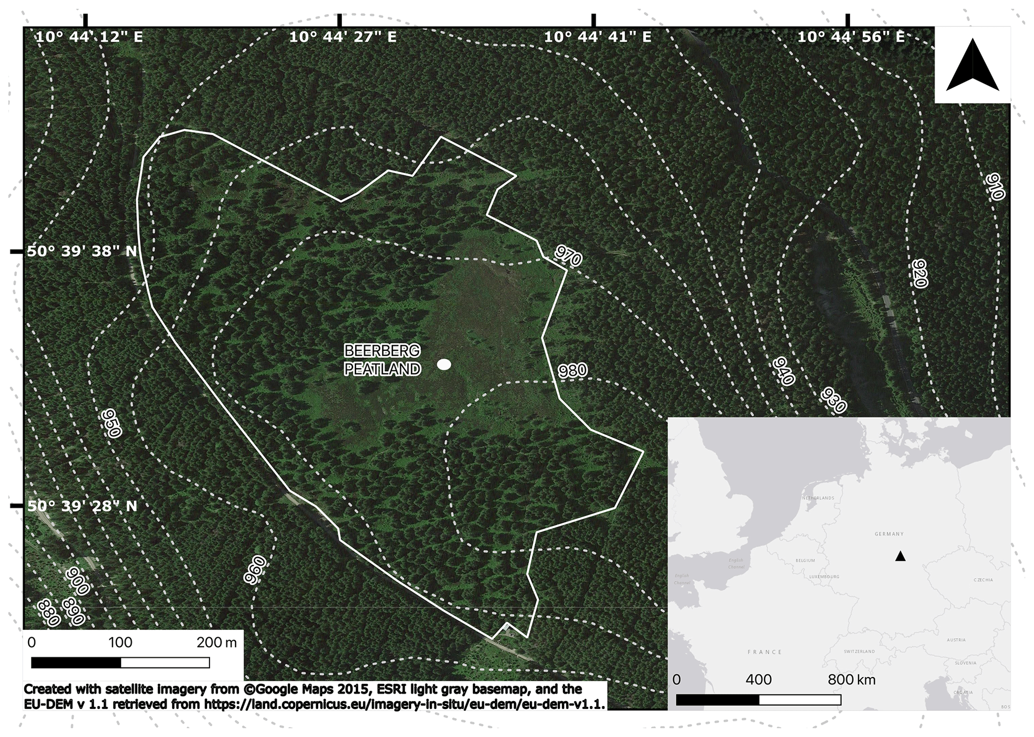
Figure 1Map showing the sampling spot in the Beerberg peatland (area within continuous white boundary), with the contour lines and inset showing the location in continental Europe.
2.1 Study area and sampling
The Beerberg peatland (50∘39′32′ N, 10∘44′36′′ E; 983 m) is a raised ombrotrophic peat bog at the summit of the Großer Beerberg in the Thuringian Forest (Germany) and is part of the Vessertal–Thuringian Forest Biosphere Reserve (Fig. 1). The underlying bedrock is rhyolite (Lützner et al., 2012). Annual precipitation is estimated to be 1300 mm (Görner et al., 1984), and the mean annual temperature is 4 ∘C (Jeschke and Paulson, 2000). While the Beerberg peatland has been under nature protection status since 1939, previously some of the peat was used as fuel for glass manufacturing. Consequently, the peatland was partially drained and reforested with spruce trees in the 19th and 20th centuries. Later, in particular after 1990, drainage trenches were filled and spruce trees were removed to prevent further drying of the peat (Thüringer Landesanstalt für Umwelt und Geologie, 2002). Current vegetation includes Sphagnum mosses, such as S. fuscum, S. magellanicum (s.l.), S. angustifolium, and S. capillifolium; tree species Picea abies, Pinus sylvestris, Betula pendula, and Betula pubescens; and other plants common in partially disturbed bogs, such as Calluna vulgaris, Eriophorum vaginatum, and Polytrichum strictum.
Sampling was completed in October 2019. Two Russian peat corers (5 cm diameter, Eijkelkamp, Giesbeck, the Netherlands; 7 cm diameter, self-made) were used to alternately core two small hummocks within an approximately 20 cm distance to a depth of 340 cm. Overlapping core sections were taken from 90–100, 175–190, and 290–320 cm. The overlapping sections were correlated by sampling depth and stratigraphy, and for the elemental and biomarker analyses, the overlapping samples were treated as replicates, and the averages of the results were calculated.
2.2 Elemental analysis
For elemental analysis, samples were taken at 5 cm intervals, with a few exceptions due to visibly distinct layers in the peat at 10–12, 170–172, 270–272, 325–327, 327–328, and 337.5–340 cm. The samples were freeze-dried to a constant weight and subsequently milled to a fine powder using a horizontal ball mill (MM 400, Retsch). Approximately 1 mg of material per sample was used for the elemental analysis. Carbon and nitrogen concentrations (C, N), as well as stable C isotope values (δ13C), were measured using an elemental analyzer isotope ratio mass spectrometer (EA-IRMS; FLASH 2000 HT Plus, linked by ConFlo IV to DELTA V Plus IRMS; Thermo Fisher Scientific). Calibration was carried out using caffeine (Merck, Germany) and a soil reference material from a Chernozem (Harsum, Germany; see black carbon reference materials, https://www.geo.uzh.ch/en/units/2b/Services/BC-material/Environmental-matrices.html, last access: 20 March 2023). At least two analytical replicates were measured for all samples.
2.3 Radiocarbon dating
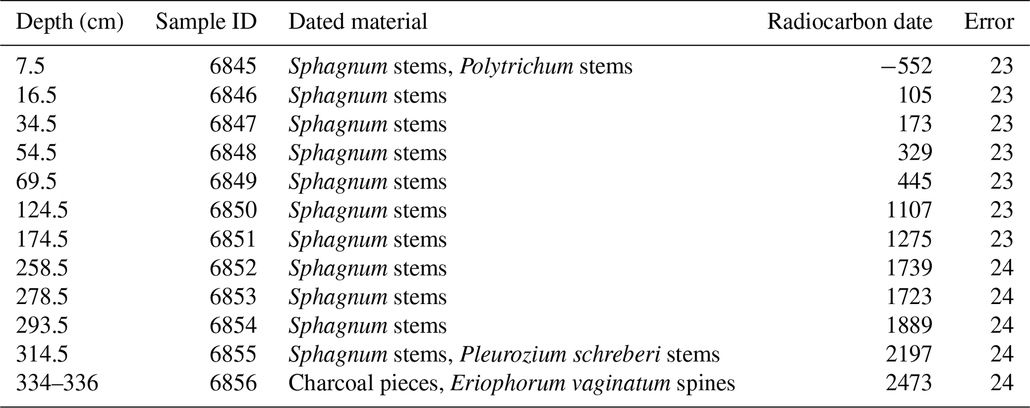
Handpicked plant remains (Table A1) were selected from 12 depths (7.5, 16.5, 34.5, 54.5, 69.5, 124.5, 174.5, 258.5, 278.5, 293.5, 314.5, and 334–336 cm). These were cleaned by an acid–alkali–acid treatment and combusted at 900 ∘C to produce CO2, which was reduced to graphite. The carbon isotope composition was measured by accelerator mass spectrometry (AMS) at the Institute of Ion Beam Physics at the Swiss Federal Institute of Technology (Zurich, Switzerland) using the 0.2 MV MICADAS facility.
2.4 Macrofossil analysis
Plant macrofossils were analyzed at 4 cm resolution (n=70, 1 cm thick peat slices) using samples with a volume of approximately 8 cm3. The samples were washed and sieved under a warm-water current over 0.20 mm mesh screens. The percentage of individual fossils of vascular plants and brown mosses was estimated, and the fossil carpological remains and vegetative fragments (leaves, rootlets, epidermis) were identified using identification keys (Smith, 2004; Mauquoy and Van Geel, 2007) and compared with recently collected specimens. S. capillifolium and Sphagnum rubellum were grouped together (as S. capillifolium/rubellum) due to the difficulty in differentiating them in fossil state. Both species are typical ombrotrophic mosses that occur together in relatively dry hummocks or lawns (Hölzer, 2010), with S. rubellum preferring moister habitats (Hölzer, 2010). Similarly, Sphagnum medium and Sphagnum divinum (in the past assigned to S. magellanicum; see Laine et al., 2018) are expressed as S. medium/divinum because it was impossible to distinguish them based on morphological features in fossil state.
2.5 Pollen analysis
For pollen analysis, the core was sampled at 2.5, 6.5, 9.5, and then 5 cm intervals starting at a depth of 12.5 cm, ending with a total of 69 samples. At each depth, a volume of 2 cm3 was extracted and subjected to standard laboratory procedures for pollen analyses (Berglund and Ralska-Jasiewiczowa, 1986). Samples were treated with 10 % hydrochloric acid (HCl) to dissolve carbonates, heated in 10 % potassium hydroxide (KOH) to remove humic compounds, and finally soaked in 40 % hydrofluoric acid (HF) for at least 24 h to remove the mineral fraction. One Lycopodium tablet (10 679 spores; produced by Lund University) was added to the samples (Stockmarr, 1971). Sample slides were analyzed using an Eclipse 50i upright microscope and counted to a sum of at least 500 arboreal pollen (AP) grains. However, due to the high peat accumulation rate, this sum was not achieved in 33 samples, including 7 samples in which a 100 AP sum was not achieved. Pollen taxa were identified using atlases (Beug, 1961; Moore et al., 1991) and the reference grains owned by the Institute of Geoecology and Geoinformation, Adam Mickiewicz University, Poznań. Selected non-pollen palynomorphs (NPPs), such as fungi and algae, and microscopic charcoal particles (size fractions: 0.01–0.1 mm; > 0.1 mm) were also counted. Microscopic charcoal particles were counted until their number summed with simultaneously counted Lycopodium spores reached 200 (Finsinger and Tinner, 2005; Tinner and Hu, 2003). Palynological indicators of human impact were organized according to Behre (1981) and Gaillard (2013).
2.6 Biomarker analysis
For biomarker analysis, the same samples were used as for the elemental analysis. Soxhlet extraction was performed using 468 mg to 758 mg of the milled peat samples, as described by Wiesenberg and Gocke (2017). Briefly, total lipids were extracted over approximately 30 h with dichloromethane(DCM) : methanol(MeOH) (93:7, ). These extracts were then separated sequentially into three fractions containing, respectively, neutral components including n-alkanes and n-alkanols, n-fatty acids, and polar and high-molecular-weight compounds. For the separation, a glass column containing silica 60 + 5 % potassium hydroxide (KOH), 63–200 µm, was used along with the solvents DCM, DCM : formic acid (99:1, ), and DCM : MeOH (1:1, ). The neutral fraction was further separated into aliphatic, aromatic, and heterocompound fractions. For this, a pasteur pipette containing activated silica gel (100 Å, 70–230 mesh, dried for at least 8 h at 110 ∘C) was used along with the solvents n-hexane, n-hexane : DCM (1:1, ), and DCM : MeOH (93:7, ).
Prior to measurement, an internal standard of deuterated n-eicosanoic acid (D39C20; Cambridge Isotope Laboratories, Inc.) was added to the fatty acid fraction, which was then methylated using a boron trifluoride–methanol solution (CAS no. 373-57-9, Sigma-Aldrich). Additionally, an internal standard of deuterated n-octadecanol (D37C18; Cambridge Isotope Laboratories, Inc.) was added to the heterocompound fraction, containing n-alkanols, which was then silylated using N,O-bis(trimethylsilyl)acetamide (BSA) (CAS no. 10416-59-8, Sigma-Aldrich). An internal standard of deuterated n-tetracosane (D50C24; Cambridge Isotope Laboratories, Inc.) was added to the aliphatic fraction before analysis. The n-alkanes, n-alkanols, and n-fatty acids were quantified on a gas chromatograph (GC; Agilent 7890B) equipped with a multimode inlet and a flame ionization detector (FID). Compound identification was performed on the Agilent 6890N GC equipped with a split–splitless injector coupled to the Agilent 5973 mass selective (MS) detector. Both instruments were equipped with a DB-5MS column (50 m × 0.2 mm × 0.33 µm) and 1.5 m deactivated pre-column, with helium as the carrier gas (1 mL min−1). The GC oven temperature for n-alkanes was held at 70 ∘C for 4 min and increased to 320 ∘C at a rate of 5 held for 50 min. For n-fatty acids and n-alkanols, the temperature was held at 50 ∘C for 4 min, then increased to 150 ∘C at a rate of 4 , and finally increased to 320 ∘C at 3 held for 40 min. The samples (1 µl) were always injected in splitless mode. The gas chromatograph–mass spectrometer (GC–MS) was operated in electron ionization mode at 70 eV and scanned from 50–550. Individual compounds were identified through comparison of mass spectra with those of external standards and from the NIST and Wiley mass spectra library.
2.7 Data processing and analysis
2.7.1 Data entry, processing, and analysis
Data were entered, organized, and screened in Microsoft Excel. Subsequent data processing and analysis were conducted in R version 4.0.4 (R Core Team, 2023). The data were combined in five tables, one each for the radiocarbon dating, elemental analysis, plant macrofossils, pollen, and biomarker composition. In each table, each row represents one depth and each column one parameter. All data are available at Pangaea via https://doi.org/10.1594/PANGAEA.961142.
2.7.2 Elemental analysis
The mean and standard error were calculated for the analytical replicates used in the elemental analysis. To be consistent across all of the data interpretation and to determine the locations of potential climate and vegetation changes in the core, we applied a hierarchical clustering analysis most commonly performed on vegetation abundance data. We used the vegan (Oksanen et al., 2022) and rioja (Juggins, 2022) R packages. The Euclidean distance was determined using the concentrations of C and N, the ratio, and the C stable isotope values in the dist function. A constrained hierarchical clustering approach (CONISS; Grimm, 1987) was performed on the dissimilarity using the chclust function, with clusters constrained by depth. The number of zones was determined using the broken-stick model (MacArthur, 1957; Bennett, 1996) with the bstick function.
2.7.3 Radiocarbon dating
An age–depth model was developed using the Bacon model (Blaauw and Christen, 2011), as implemented in the rbacon package (Blaauw et al., 2021). The uppermost radiocarbon date was excluded from the age–depth model, as it was from a sample within 10 cm of the surface, and the yielded date of −552 yr BP ± 23 is too young and stratigraphically inconsistent with the rest of the core and represents a postbomb peak of atmospheric 14C, following nuclear weapon testing in the 1950s and 1960s (Table A1). As a constraint, an estimated surface sample age of −70 yr BP ± 5 was added. IntCal20 was used as the calibration curve (Reimer et al., 2020), and NH1 was used as the calibration curve for postbomb dates (Hua et al., 2013). All of the dates referred to in the following sections are the mean values returned by the age–depth model, which were calculated at 1 cm resolution.
2.7.4 Macrofossil
A CONISS cluster analysis (Grimm, 1987) was performed on the macrofossil abundance data. In contrast with the elemental data, the Bray–Curtis dissimilarity was calculated as this is a better measure for purely compositional data. This was completed using the vegdist, chclust, and bstick functions described in the previous section.
2.7.5 Pollen and microcharcoal
The microscopic charcoal accumulation rate (CHARmicro; unit: ) was calculated as follows:
in which CHACmicro is the concentration of the microscopic charcoal particles (unit: particles cm−3), and ARdeposits is the peat or sediment accumulation rate (unit: cm yr−1) (Davis and Deevey, 1964).
Pollen percentages were calculated as taxon percentages with
where TPS indicates the total pollen sum, including the AP and non-arboreal pollen (NAP) taxa and excluding the local taxa (i.e., aquatic, wetland, and spore-producing).
TILIA software was used to plot the diagram presenting the results of the palynological analysis (Grimm, 1993). We performed a CONISS cluster analysis as described in the previous section using the absolute pollen counts. Only taxa present in at least three samples and that reached at least 3 % relative abundance in one sample were included. Non-pollen palynomorphs and coprophilous fungi were not included in the analysis.
2.7.6 Biomarker
Biomarker amounts are reported as absolute concentrations in micrograms per gram. The total lipid extract (TLE) was calculated in milligrams per gram. The carbon preference index (CPI) (Marzi et al., 1993) and average chain length (ACL) (Poynter et al., 1989) were also calculated for the n-alkanes using the following equations:
where Cx is the concentration of each lipid containing x carbon atoms; n and m are the chain lengths of the starting and ending lipids divided by 2, respectively (note that both 2n and 2m should be even numbers). For the n-alkanes, m is 11 and n is 15.
For the n-alkanols and n-fatty acids, the formulas were slightly adjusted to
For the n-alkanols, m is 10 and n is 14. For the n-fatty acids, m is 10 and n is 16.
A number of indicative ratios have been developed to help interpret biomarker data, particularly for n-alkanes. We applied many of these to our data to see which was the most applicable in the Beerberg setting. The Paq (Ficken et al., 2000) and Pwax (Zheng et al., 2007) proxies have previously been used in sediments to differentiate between aquatic macrophyte and terrestrial plant input and in peatlands to infer past water levels with high Paq values associated with a higher water table and high Pwax values associated with a lower water table (e.g., Zheng et al., 2007; Zhou et al., 2005; Nichols et al., 2006; Andersson et al., 2011).
Andersson et al. (2011) found that Paq and Pwax could be misleading if S. fuscum and Betula species were present in the peat due to their relatively high abundances of the C23 homologue. They derived the ratio of to correct for these inputs, and as both S. fuscum and Betula species were present at the Beerberg site, this ratio was included. The ratio of n-alkanes () was also calculated, as this has been used in peatland settings before to determine shifts in Sphagnum species (McClymont et al., 2008). Furthermore, and were calculated, and other studies have used these to distinguish Sphagnum species in peat settings (e.g., Ronkainen et al., 2013). Far fewer ratios have been identified for n-alkanols and n-fatty acids. Nevertheless, we tested , (Zheng et al., 2011), and for the n-alkanols and (Zheng et al., 2007) and for the n-fatty acids.
A CONISS cluster analysis (Grimm, 1987) was performed on the absolute concentrations of the measured homologues of the n-alkanes (C19–C33), n-alkanols (C16–C28), and n-fatty acids (C14–C32) to determine whether different phases could be distinguished using only the biomarker data. The same procedure was followed as previously described in the macrofossil and pollen sections.
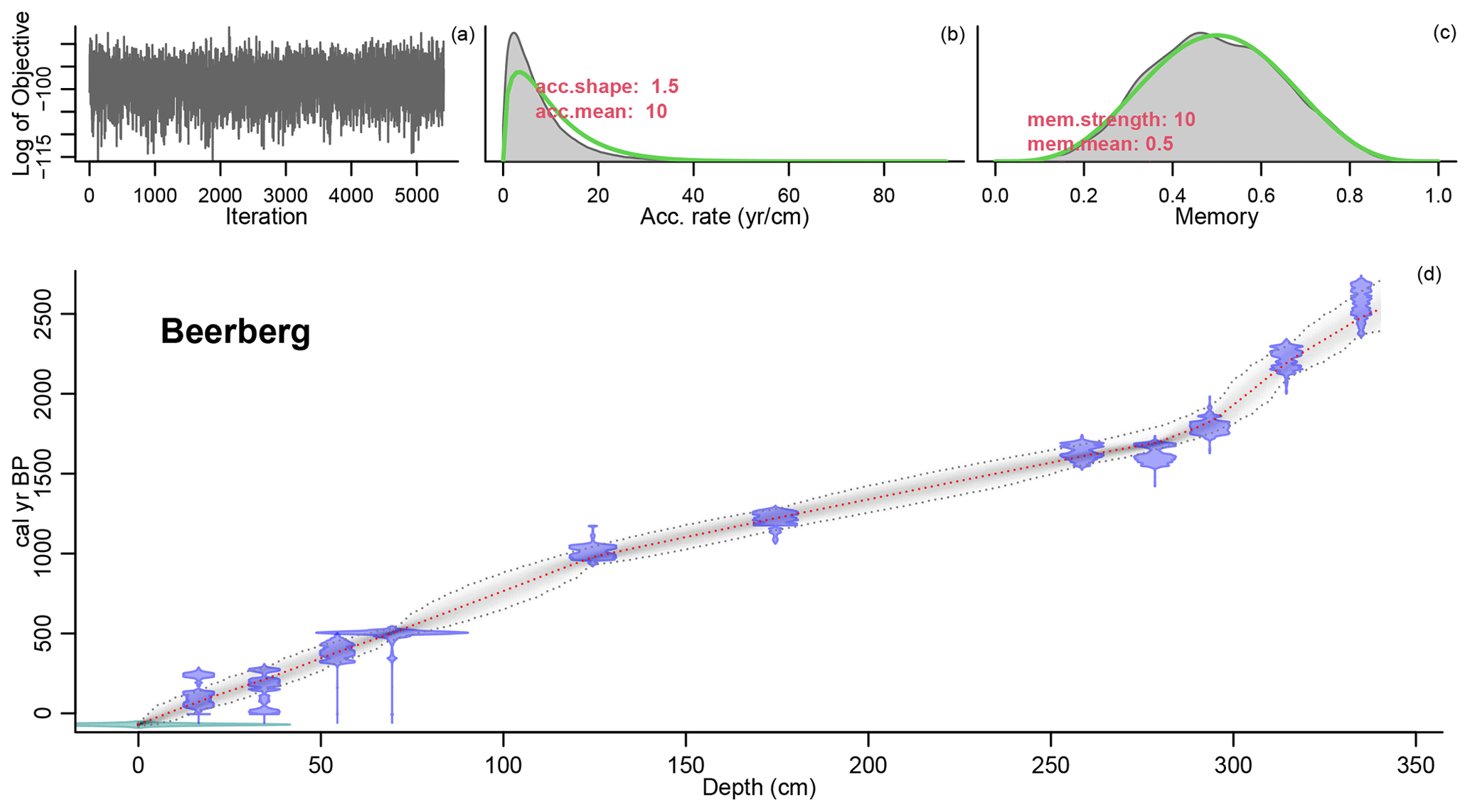
Figure 2Age–depth model of the Beerberg core. For precise radiocarbon dates, see Table A1. The age–depth model is shown in the main graph (d). The distribution of the calibrated 14C dates is shown in blue, and the estimated surface age of −70 cal yr BP is shown in green. The wider the distribution, the less precise the dates. The dashed red curve shows the mean ages derived from the model, and the dashed grey curves represent the 95 % confidence intervals. The top three graphs in the figure show the fit of the Markov chain Monte Carlo (MCMC) iterations (a), the accumulation rate (yr cm−1) with prior (green) and posterior (grey) distributions (b), and the prior (green) and posterior (grey) distributions for the memory (c) or how much the accumulation rate is able to change from one depth to the next. For more information on the Bacon model, see Blaauw and Christen (2011).
3.1 Radiocarbon dating
The age–depth model that best matched the data in this study used a mean accumulation rate of 1 mm yr−1. The resulting curve is visualized in Fig. 2. There are three clear phases with distinct accumulation rates in the model: 0.66 mm yr−1 from 340–293.5 cm (2528–1826 cal yr BP), 1.99 mm yr−1 from 293.5–124.5 cm (1826–978 cal yr BP), and 1.27 mm yr−1 from 124.5–0 cm (978–present). Hence, the changes in accumulation rates correspond with the dated samples at 293.5 and 124.5 cm.
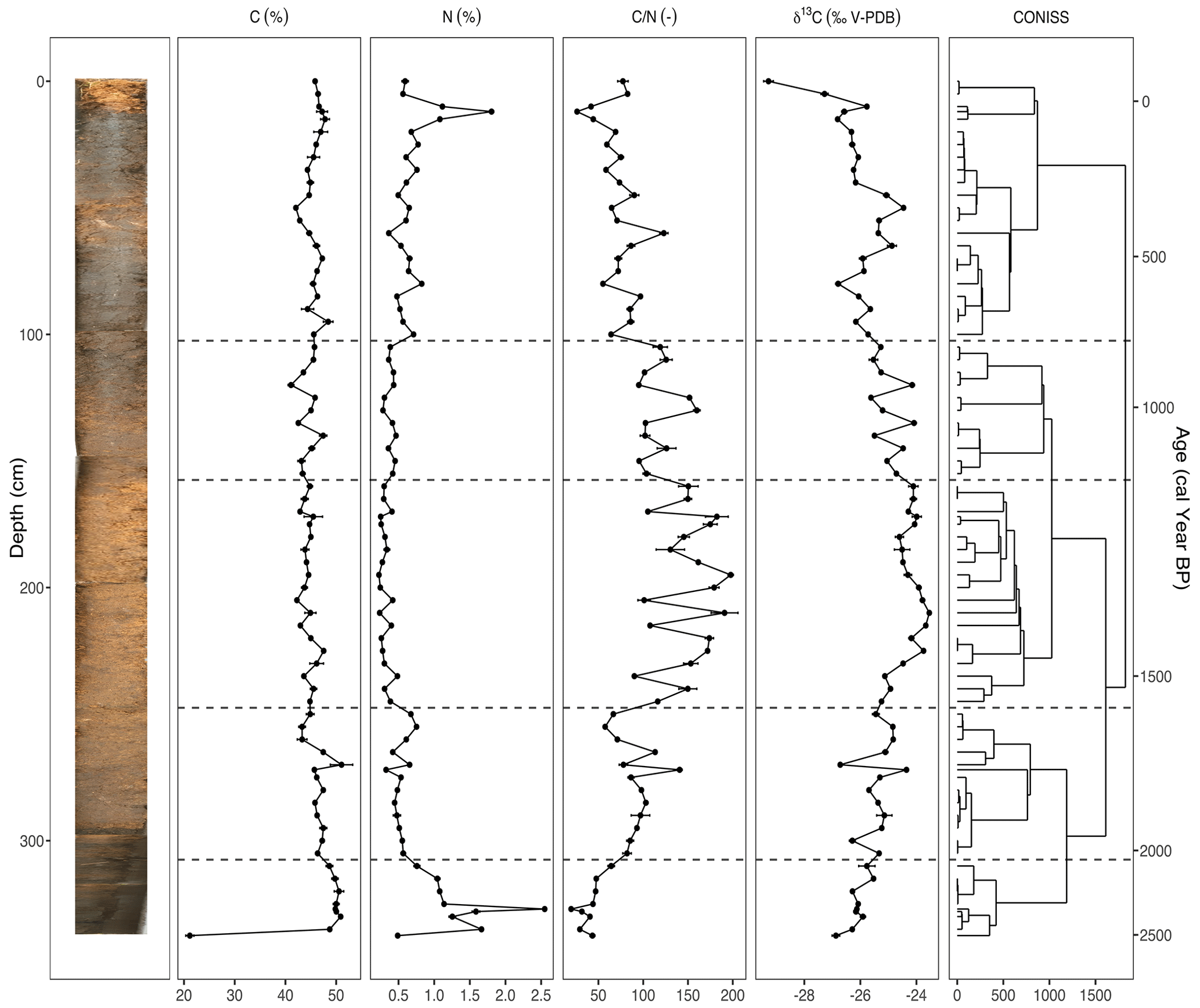
Figure 3The carbon (C) and nitrogen (N) concentrations, ratio, and stable carbon isotope composition (δ13C) plotted against depth (cm) and modeled age (cal yr BP), including the resulting dendrogram of the CONISS analysis and phase boundaries indicated at 2113 cal yr BP (310 cm), 1569 cal yr BP (250 cm), 1151 cal yr BP (160 cm), and 809 cal yr BP (105 cm). An image of the sampled core is inset on the left. Two analytical replicates of each sample were measured. Error bars showing standard error are present for the C and N concentrations, ratio, and δ13C values.
3.2 Elemental analysis
The results of the elemental analysis are shown in Fig. 3. The CONISS analysis based on Euclidean distance resulted in five zones: 2528–2113 cal yr BP (Phase I-G), 2113–1569 cal yr BP (Phase II-G), 1569–1151 cal yr BP (Phase III-G), 1151–809 cal yr BP (Phase IV-G), and 809 cal yr BP–present (Phase V-G). The transitions between phases appear to be the most correlated with changes in the δ13C values. The carbon concentration (C) ranged from 41.1 %–51.1 %, with one exceptionally low value of 21.1 % in the basal sample of Phase I-G (340–310 cm). The nitrogen concentration (N) also had a sharp peak of 2.5 % in Phase I-G at 2368 cal yr BP (327 cm). Both the ratio and the δ13C values increased during Phase I-G to 64.3 and −25.8, respectively. This increasing trend continued into Phase II-G for both (310–250 cm), with the ratio averaging 90.2 and δ13C averaging −25.4. N values decreased, while C stayed stable. During Phase III-G (250–160 cm), the ratio fluctuated rapidly between 90.1–197.7, likely due to relatively small shifts in N. This phase contained the highest values with low N as well as less negative δ13C values, ranging from −23.5 to −25.2. In Phase IV-G (160–105 cm), and δ13C began to decrease, ranging from 95.1–159.8 and −24.1 to −25.6, respectively. In Phase V-G (105–0 cm), the ratio continued to decrease as N values increased, reaching a peak of 2 % at 102 cal yr BP (20 cm). While the δ13C value of the topmost sample at −29.3‰ was particularly low, there was also an interval of increasing values from 593 cal yr BP (80 cm) to 345 cal yr BP (50 cm), reaching a local maximum of −24.5.
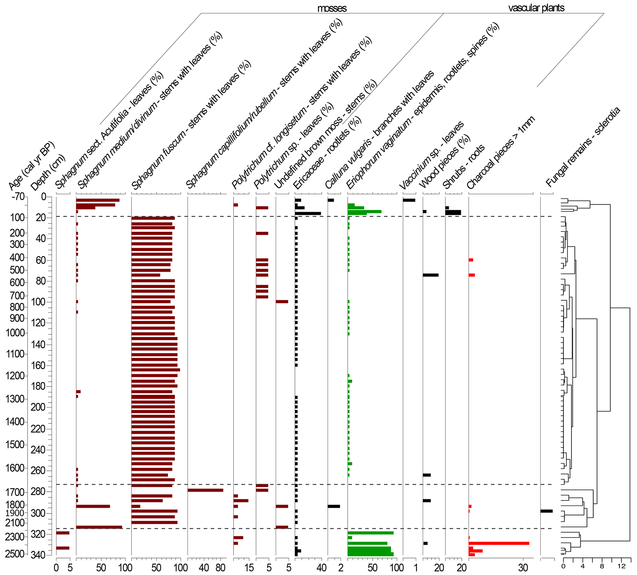
Figure 4Plant macrofossil diagram presenting local vegetation development in the Beerberg peatland. Taxa with percentages are estimated volume percentages; the others are absolute counts (note scale differences on the x axes). The resulting dendrogram of the CONISS analysis is on the right with phase boundaries indicated at 2251 cal yr BP (318.5 cm), 1671 cal yr BP (273.5 cm), and 64 cal yr BP (15.5 cm).
3.3 Macrofossil analysis
Based on the macrofossil analysis, the primary peat-forming species were S. fuscum and S. medium/divinum (Fig. 4). S. fuscum was dominant over most of the core, from 2086–106 cal yr BP (308.5–20.5 cm), with S. medium/divinum taking over in more recent layers (47 to −48 cal yr BP; 13.5–3.5 cm). Additionally, E. vaginatum was an important species with two major periods from 64 to −4 cal yr BP (15.5–7.5 cm) and 2528–2251 cal yr BP (340–318.5 cm).
The CONISS analysis based on the Bray–Curtis dissimilarity resulted in four significant phases (Fig. 4). Phase I-M (2528–2251 cal yr BP) is characterized by a high abundance of E. vaginatum as well as a relatively large amount of macrocharcoal (here charred wood pieces), especially at a depth of 328.5 cm (2388 cal yr BP). In Phase II-M (2251–1671 cal yr BP), S. fuscum was dominant. In Phase III-M (1671–64 cal yr BP), S. fuscum remained dominant, but there was also a small but relatively steady presence of E. vaginatum and Ericaceae rootlets. In Phase IV-M (64 cal yr BP–present), S. medium/divinum replaced S. fuscum, and there was an increase in Ericaceae rootlets as well as E. vaginatum.
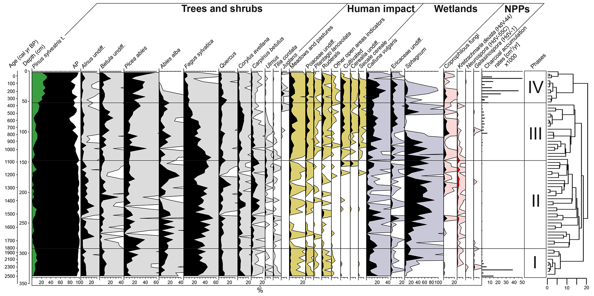
Figure 5Diagram of selected pollen taxa, NPPs, and microscopic charcoal influx (CHARmicro), including the resulting dendrogram of the CONISS analysis and phase boundaries indicated at 1816 cal yr BP (292.5 cm), 1092 cal yr BP (147.5 cm), and 366 cal yr BP (52.5 cm).
3.4 Pollen analysis
The CONISS cluster analysis of the complete pollen assemblage resulted in a separation into four phases, each representing a different regional vegetation composition (Fig. 5).
3.4.1 Phase I-P (2528–1816 cal yr BP)
At the beginning of Phase I-P (340–292.5 cm), forests were dominated by Fagus sylvatica (pollen: 24 %–44.5 %) (Fig. 5). P. sylvestris, Betula undiff., Alnus undiff., Abies alba, and P. abies also constituted a high proportion within the arboreal pollen. The latter two species significantly increased their percentage approaching 1810 cal yr BP. This time interval was characterized by high fire activity events as indicated by high CHARmicro (max 6035–38 139 ) values and the presence of Neurospora, as well as Gelasinospora ascospores between 2500–2300 cal yr BP (Stivrins et al., 2019). Towards the end of the phase, Sphagnum began to increase, indicating a shift to moss-dominated peat.
3.4.2 Phase II-P (1816–1092 cal yr BP)
During the second phase, the forests were dominated by F. sylvatica (18 %–54.5 %) (Fig. 5). A. alba and P. abies were the main components of coniferous forests. A significant decline in F. sylvatica occurred between 1280–1210 cal yr BP. During this phase, A. alba and Quercus reached their highest proportion in the forest. Based on indicator pollen counts, human impact in this phase was the weakest along the entire paleorecord. At the end of this phase, crop introduction in the region was observed, mirrored by an increase in Cerealia pollen share. The stable conditions prevailed at that time in the peatland, which was dominated by Sphagnum and C. vulgaris as well as other Ericaceae species.
3.4.3 Phase III-P (1092–366 cal yr BP)
Throughout this zone, arboreal pollen declined from 97.5 % to 77.5 % between 1090–570 cal yr BP (Fig. 5). A substantial decline in late successional species such as F. sylvatica and C. betulus was observed, especially at the end of this phase. Along with the decrease in the proportion of these species, pioneer trees such as P. sylvestris, Betula, and Corylus avellana constituted an increasing proportion among the woodlands. During this phase, a constant share of cultivated indicators (mostly Cerealia undiff. and Secale cereale) was also recorded, especially from 740 cal yr BP. At the same time, a sharp increase in CHARmicro, as well as coprophilous fungi taxa, was observed. This corresponded with a sharp decrease in the proportion of Sphagnum (740–570 cal yr BP), the values of which increased again at the end of this phase. At the same time, the disappearance of K. deusta was noticeable during this phase.
3.4.4 Phase IV-P (366 cal yr BP–present)
The major deciduous trees that previously formed the stand gradually withdrew from the site, as manifested by decreasing percentages of F. sylvatica (from 18 % to 4.4 %), Quercus, and Corylus avellana (Fig. 5). P. abies and P. sylvestris reached their highest proportions in the forest (13.5 %–58 % and 21 %–32.5 %, respectively), whereas A. alba seemed to decline completely, as evidenced by the disappearance of its percentage share.
3.5 Biomarker analysis
The TLE following Soxhlet extraction ranged between 20–66 mg g−1, with an average of 35mg g−1. n-Alkanes were measured with chain lengths from C19 to C33, n-alkanols from C16 to C28, and n-fatty acids from C14 to C32. The total abundance of n-alkanes ranged from 80–1112 µg g−1, n-alkanols from 47–469 µg g−1, and n-fatty acids from 260–4224 µg g−1. Overall, the signatures are indicative of higher-plant source material (Eglinton and Hamilton, 1967). The CONISS cluster analysis identified four phases with boundaries at 35 cal yr BP (12 cm), 809 cal yr BP (105 cm), and 1657 cal yr BP (270 cm) (Fig. 6). These four phases are described in the following sub-sections.
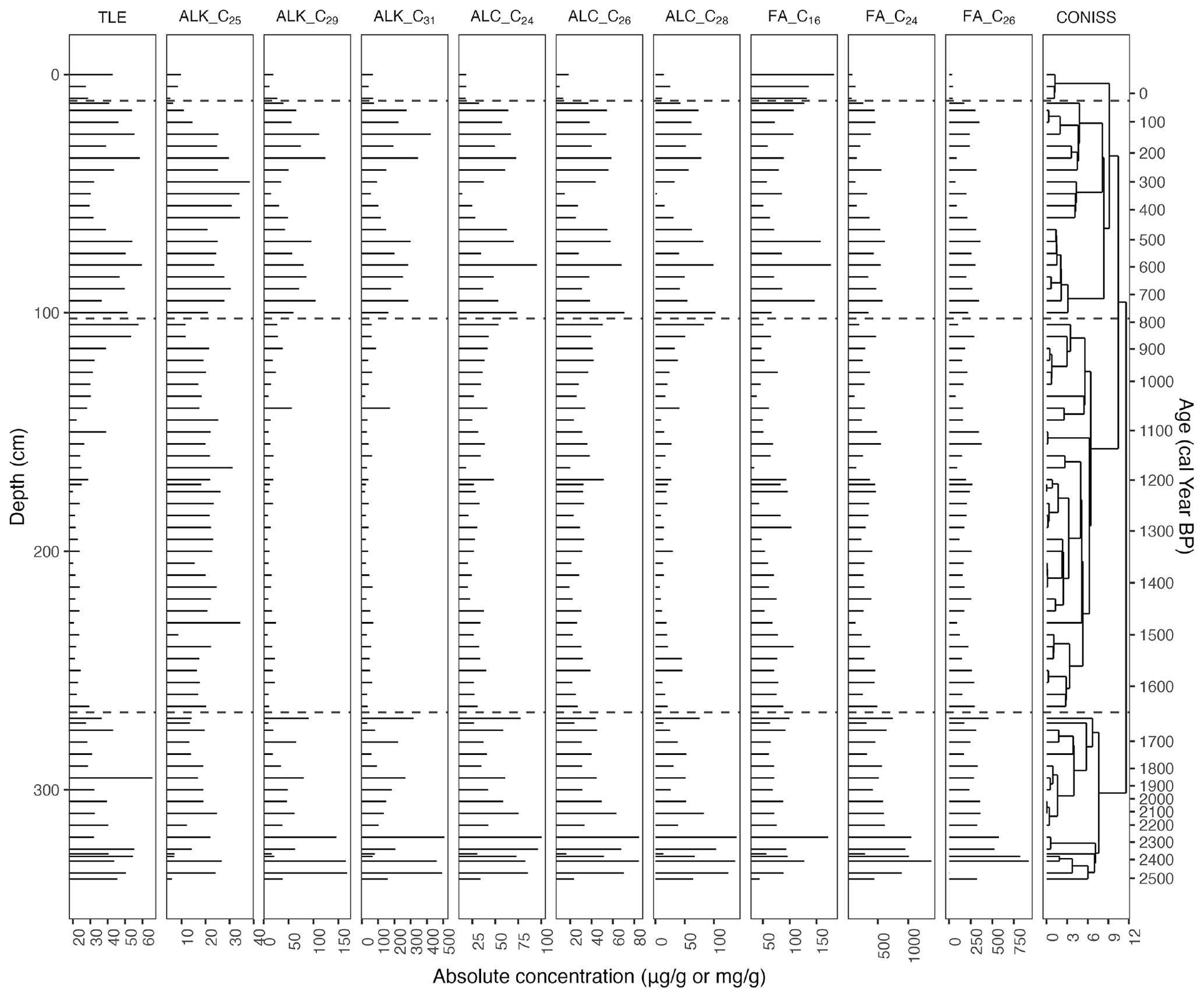
Figure 6Absolute concentration (µg g−1) values for the most abundant homologues of the n-alkanes (ALK; C29, C31, and C33), n-alkanols (ALC; C24, C26, and C28), and n-fatty acids (FA; C22, C24, and C26) as well as the C23 and C25 n-alkanes and C16 n-fatty acid. On the right is the resulting dendrogram of the CONISS analysis of the complete biomarker values with phase boundaries indicated at 35 cal yr BP (12 cm), 809 cal yr BP (105 cm), and 1657 cal yr BP (270 cm).
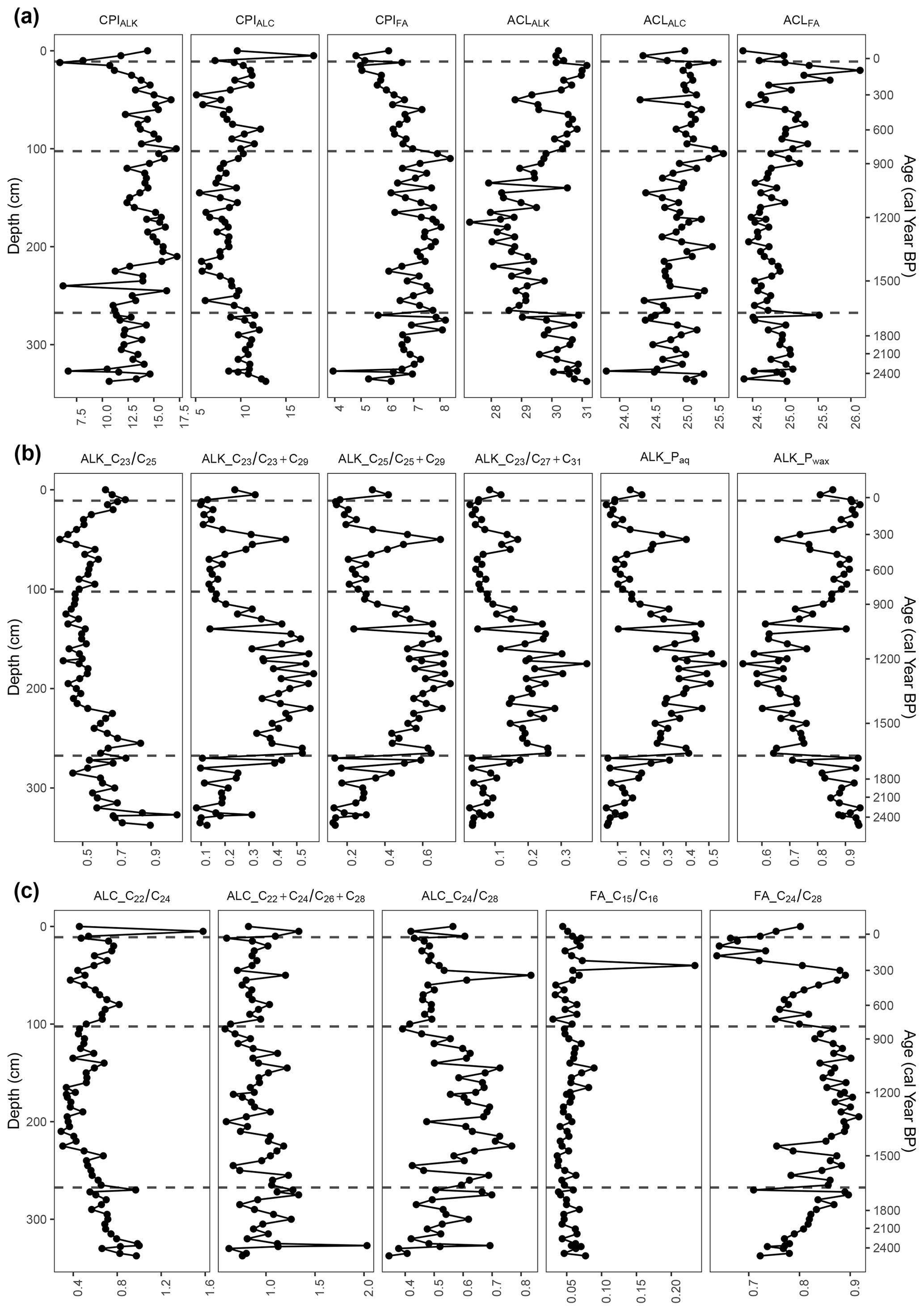
Figure 7Carbon preference index (CPI) and average chain length (ACL) values of n-alkanes (ALK), n-alkanols (ALC), and n-fatty acids (FA) and n-alkane, n-alkanol, and n-fatty-acid ratios. The four phases from the cluster analysis are indicated at 35 cal yr BP (12 cm), 809 cal yr BP (105 cm), and 1657 cal yr BP (270 cm).
3.5.1 Phase I-B (2528–1657 cal yr BP)
At the very beginning of the first phase, the TLE was relatively high but began to decrease around 2272 cal yr BP (320 cm). The most abundant homologues for the n-alkanes and n-fatty acids were consistently C31 (33–508 µg g−1) and C24 (293–1376 µg g−1), respectively (Fig. 6). For the n-alkanols, the most abundant homologues varied between C22, C24, C26, and C28 (14–139 µg g−1). The CPI of the n-alkanes (CPIALK) ranged from 6.7–14.6, averaging 12.3 (Fig. 7); that of the n-alkanols (CPIALC) from 8.7–12.8, averaging 10.7; and that of the n-fatty acids (CPIFA) from 3.9–8.2, averaging 6.7. The ACL of the n-alkanes (ACLALK) varied from 29.0–31.2, averaging 30.3; that of the n-alkanols (ACLALC) from 23.8–25.3, averaging 24.8; and that of the n-fatty acids (ACLFA) from 24.4–25.1, averaging 24.9 (Fig. 7). Of the n-alkane ratios, Paq ranged from 0.05–0.33, averaging 0.13; Pwax from 0.71–0.95, averaging 0.88; from 0.02–0.18, averaging 0.07; from 0.08–0.44, averaging 0.20; from 0.13–0.59, averaging 0.27; and from 0.44–1.05, averaging 0.67. While and Pwax generally decreased throughout the phase, Paq, , , and generally increased (Fig. 7). The n-alkanol ratios ranged from 0.55–1.00, averaging 0.75; from 0.62–2.03, averaging 1.03; and from 0.34–0.70, averaging 0.52. Generally, and increased throughout the phase, while decreased. The n-fatty-acid ratios ranged from 0.04–0.08, averaging 0.05, and from 0.72–0.90, averaging 0.81. stayed nearly the same through the phase, while increased.
3.5.2 Phase II-B (1657–809 cal yr BP)
In the second phase, the TLE decreased further until it began to increase around 1209 cal yr BP (172 cm). The most abundant homologues for the n-alkanes and n-fatty acids consistently remained C31 (19–317 µg g−1), with one exception of C25 (26 µg g−1) at 1223 cal yr BP (175 cm) and C24 (123–747 µg g−1), respectively (Fig. 6). For the n-alkanols, the most abundant homologues varied between C24, C26, and C28 (6–77 µg g−1). All of the CPI values remained well over 1 (Fig. 7). The average of ACLALK decreased slightly to 28.9, while the other ACL average values remained nearly the same. The averages of Paq, , , and increased to 0.35, 0.40, 0.55, and 0.19, while the averages of Pwax and decreased to 0.70 and 0.53. The averages of the n-alkanol ratios and decreased to 0.49 and 0.92, while that of increased to 0.61. The averages of the n-fatty-acid ratios stayed nearly the same. During this phase, many of the proxies followed a similar curve or its inverse, reaching either a peak or a dip near the middle of the phase. These include ACLALK, , , , Paq, Pwax, n-alkanol , and n-fatty acid (Fig. 7).
3.5.3 Phase III-B (809–35 cal yr BP)
In the third phase, the TLE increased, though it had a slight dip from 466 to 259 cal yr BP (65–40 cm). Following the dip, the TLE increased again to the same level as at the beginning of the phase. The most abundant homologues for the n-alkanes and n-fatty acids were consistently C31 (55–423 µg g−1) and C24 (136–619 µg g−1), with one exception of C26 (242 µg g−1 at 178 cal yr BP; 30 cm), respectively (Fig. 6). For the n-alkanols, the most abundant homologues varied between C24, C26, and C28 (3–103 µg g−1). All of the CPI values again remained over 1 (Fig. 7). The averages of the ACL values all increased slightly (ALK: 30.3; ALC and FA: 25.1). The averages of Paq, , , , and decreased to 0.15, 0.52, 0.19, 0.31, and 0.07, while the average of Pwax increased to 0.86. The average of the n-alkanol ratio increased to 0.62, while that of and decreased to 0.86 and 0.50. The average of the n-fatty-acid ratio increased due to a high peak at 250 cal yr BP (40 cm), then decreased to its previous level and stayed almost the same, and that of decreased to 0.78. During this phase, many of the proxies reached a local maximum or minimum around 345 cal yr BP (50 cm) (Figs. 6 and 7).
3.5.4 Phase IV-B (35 cal yr BP–present)
In the fourth, most recent phase, there are only four samples, so patterns are difficult to identify. The TLE initially dipped from its values in Phase III-B but was relatively high in the uppermost sample (43 mg g−1). The most abundant homologues for the n-alkanes and n-fatty acids were consistently C31 (42–75 µg g−1) and C24 (76–263 µg g−1), respectively (Fig. 6). For the n-alkanols, the most abundant homologues varied between C22, C24, C26, and C28 (8–43 µg g−1). The CPI values all remained above 1 (Fig. 7). The average ACL values remained almost the same. The average values of the n-alkane ratios stayed nearly the same, except for , which increased from 0.52 to 0.69 (Fig. 7). The averages of the n-alkanol ratios and increased to 0.76 and 0.96, while the averages of the other n-alkanol and n-fatty-acid ratios stayed almost the same.
Table 1Phases identified with CONISS analysis of different proxies and major changes between each phase.
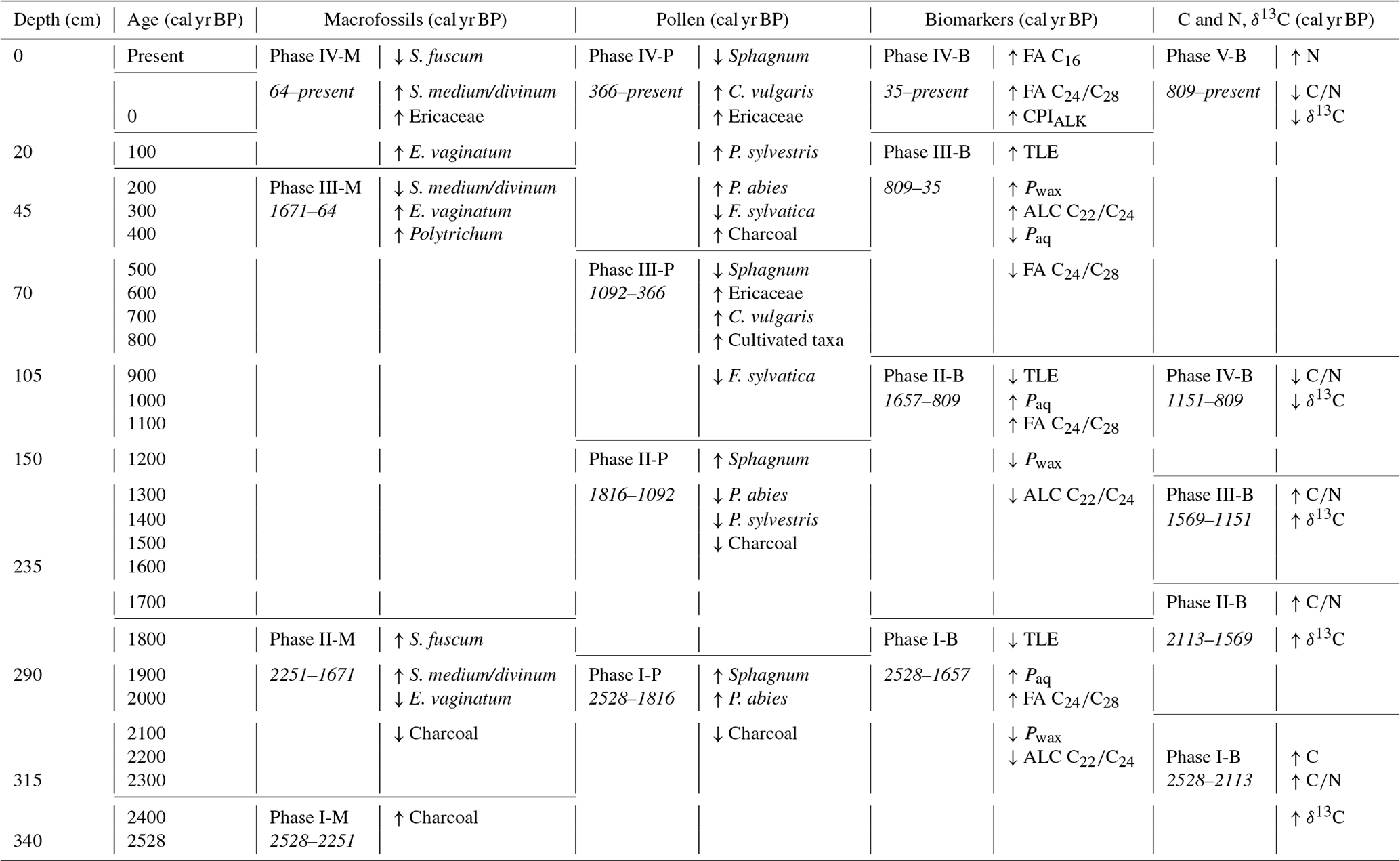
4.1 Temporal differences in trends across molecular proxies
The CONISS analysis identified different phases across all of the proxy records, though there were similar trends across most of the records (Table 1). The elemental data were split into five phases: 2528–2113, 2113–1569, 1569–1151, 1151–809, and 809 cal yr BP–present (Fig. 3). The C and N concentrations, ratio, and δ13C values are reflective of both the source material and the environmental conditions, as well as post-deposition decomposition. Therefore, although there are similarities between the patterns of the elemental data and the other proxy records, they do not match exactly.
The macrofossil data were clustered into four phases: 2528–2251, 2251–1671, 1671–64, and 64 cal yr BP–present (Fig. 4). Compared with the elemental data, the CONISS analysis identified one fewer significant zone, and while the first two phase boundaries of each proxy are within 140 cal yr BP of each other, the others do not align.
The pollen data were clustered into four phases: 2528–1816, 1816–1092, 1092–366, and 366 cal yr BP–present (Fig. 5). The pollen data reflect both a local and a regional vegetation signal, so while there are similarities between the phases based on the pollen and those based on the elemental and macrofossil data, they do not line up exactly.
The biomarker data were also clustered into four phases: 2528–1657, 1657–809, 809–35, and 35 cal yr BP–present (Fig. 6). The first three phases in the biomarker data are the most similar to those of the pollen data, while the final phase is the most closely aligned with that of the macrofossil data. The biomarker data reflect the source material and post-deposition decomposition, so some offsets to the other proxy records are expected.
Because macrofossils are conventionally seen as the most reliable proxy reflecting in situ vegetation and peat development (Birks and Birks, 2000, e.g.,), we used the phases based on the macrofossils to describe the peatland development.
4.2 Development of the Beerberg peatland
In Phase I-M, 2528–2251 cal yr BP, the vegetation is characterized by a dominant presence of E. vaginatum (Fig. 4), along with a relatively low ratio and very negative δ13C values (Fig. 3), which is typical for fen peat or transitional peat underlying bog peat (Kuhry et al., 1992; Jones et al., 2010). High fire activity during this phase was indicated by the maximum count of macrocharcoal pieces (charred wood, moss stems, Calluna leaves) (Fig. 4) occurring in this interval as well as increased CHARmicro (Fig. 5) and the presence of carbonicolus ascospores, Neurospora and Gelasinospora (Shumilovskikh and van Geel, 2020). It is likely that some of the fire events were a result of anthropogenic activity, indicated by the presence of Plantago lanceolata or ruderal communities like Artemisia or Chenopodiaceae during this phase (Fig. 5). Fires in the bog area could have initiated the peat development as initial (fen) peat could form on wet ground following fire, developing into transitional peat and then bog peat, as has been seen at other sites (e.g., Tuittila et al., 2007; Gałka et al., 2019). The pollen analysis also indicated that Fagus sylvatica was the dominant arboreal species during this time period (Fig. 5), as was also determined by Lange (1967). Although F. sylvatica is considered a fire-sensitive species (Tinner et al., 2000), it records maximum occurrence in this phase soon after the fire. This could also signify that the fire negatively affected the presence of A. alba and P. abies in contrast to F. sylvatica. The disappearance of Neurospora and Gelasinospora combined with the rapid decline in CHARmicro corresponds with the development of the Sphagnum community on peatland. This may also indicate wetter conditions on peatlands, especially during 2500–2230 cal yr BP. The increasing ratio and δ13C values towards the end of the phase (Fig. 3), as well as the initial incidences of Sphagnum (Figs. 4 and 5), indicates a shift towards more ombrotrophic conditions (Wang et al., 2015). The estimated accumulation rate during this phase (Fig. 2) is also relatively low compared with the rest of the core, likely due to the lower proportion of mosses (Stivrins et al., 2017) as it is the paludification phase, the initiation of the peatland. The biomarker data also support this interpretation, with Pwax, Paq, , , and all indicating an initial high proportion of longer-chain-length n-alkanes usually deriving from vascular plants (Fig. 7). Through the phase, the relative abundance of the shorter C23 and C25 n-alkanes (Fig. 6) increases, indicating the beginning of the peat development and an increase in the proportion of Sphagnum mosses (Baas et al., 2000; Pancost et al., 2002; Bingham et al., 2010). Of the other ratios, the n-alkanol generally decreased, while the n-fatty acid increased, potentially indicating an increase in n-alkanol C24 and n-fatty acid C24, which have previously been measured as dominant chain lengths in some Sphagnum species (e.g., Ficken et al., 1998a; Corrigan et al., 1976). Additionally, the TLE and individual biomarker absolute concentrations were relatively high compared with later phases in the core (Fig. 6). This aligns with previous research finding that, compared with vascular plant species, Sphagnum mosses produce lower outputs of lipids (Pancost et al., 2002); therefore, as the proportion of Sphagnum increases, the TLE and biomarker concentrations decrease.
Following the shift to ombrotrophic conditions, in the second phase, 2251–1671 cal yr BP, S. fuscum was dominant and the main peat-forming plant (Fig. 4). There was also a fairly steady presence of Ericaceae rootlets, though no evidence of E. vaginatum. At the beginning of this phase, there were also remnants of S. medium/divinum species as well as Polytrichum. In the pollen data, the percentage of Sphagnum spores increased rapidly, along with that of P. abies (Fig. 5). During this phase, the ratio and δ13C values began to increase (Fig. 3), indicating wetter conditions during rapid peat growth and low decomposition (Loisel et al., 2010; Kuhry and Vitt, 1996). The accumulation rate thus also began to increase during this phase (Fig. 2). In the biomarker data, the n-alkane ratios, indicating an increase in the proportion of shorter chain lengths (C23 and C25), continued to increase due to the rise in Sphagnum. This was also the case for n-fatty acid (Fig. 7). The TLE and absolute concentrations of individual biomarkers decreased from the first phase (Fig. 6), as expected with the increase in Sphagnum.
In the third phase, 1671–64 cal yr BP, S. fuscum was still dominant in the macrofossils, but a steady presence of E. vaginatum returned along with S. medium/divinum and Polytrichum in the later half of the phase (Fig. 4). The ratio and δ13C values reached their peak during this phase, indicating wet conditions and low decomposition (Loisel et al., 2010; Kuhry and Vitt, 1996). Within this interval, Phase II-P (1816–1092 cal yr BP) of the pollen assemblage is contained (Fig. 5). During this period, the presence of the parasitic fungus Kretzschmaria deusta – an indicator of tree fungal infections, often found on deciduous trees, especially on Fagus sylvatica – was recorded (Wilkins, 1934). Among other mountain sites, its presence was mostly associated with a higher proportion of F. sylvatica and other broad-leaved trees (Czerwiński et al., 2020; Kołaczek et al., 2020). The increased presence of this fungus in the past may have been related to stronger herbivore presence and/or coppicing practices and/or grazing damages (Latałowa et al., 2013; Karpińska-Kołaczek et al., 2014). However, the exact interactions between fungal infection and other disturbance factors in the past are not fully understood (Kołaczek et al., 2020). In the case of the Beerberg site, K. deusta was recorded during the period of the lowest human impact and seemed to correspond with the development of forests with a higher role of Carpinus betulus. During this period, CHARmicro values were very low, which suggests a decline in fire activity or even a lack of fires near the study site. The ratio and δ13C values generally also began to decline (Fig. 3), which in an ombrotrophic peat indicates drier conditions (Loisel et al., 2010) and increased decomposition (Kuhry and Vitt, 1996) and could be related to human impact, such as drainage of the peatland. In the forest, P. abies expanded (especially from 520 cal yr BP) and possibly replaced F. sylvatica in cleared areas (Fig. 5). This pattern has previously been observed at other sites in Germany, such as the Black Forest (Rösch, 2000; Gałka et al., 2022b). Deforestation was related to human impact, as evidenced by an increase in indicators typical of open landscapes, including meadows and pastures, such as Poaceae and Plantago lanceolata, as well as ruderal habitats (mostly Rumex acetosa/acetosella type, Artemisia, Chenopodiaceae, and Brassicaceae undiff.). Further evidence of human impact results from the steady proportion of cultivated species, as well as the increase in CHARmicro and coprophilous fungi taxa. During this phase, the biomarker records showed more variation than the macrofossils. The TLE and absolute concentrations were relatively low through the phase until around 809 cal yr BP when they began to increase; there was another dip in the TLE and most individual concentrations (excluding the n-alkanes C23 and C25) from around 466 to 259 cal yr BP, increasing again in the final part of the phase (Fig. 6). The fluctuations in TLE are likely related to a decrease and subsequent increase in Sphagnum, as well as an increase in the proportion of Ericaceae species and other vascular plants (Pancost et al., 2002) in the latter half of the phase. The biomarker ratios follow a similar pattern, with many reaching either a maximum or a minimum point around 1200 cal yr BP, including Paq, , , and , as well as the n-alkanol and n-fatty acid (Fig. 7). These ratios also showed a local maximum or minimum around 345 cal yr BP. This is also seen in the δ13C curve as well as in a color change in the peat core itself (Fig. 3). All of these proxies appear to be indicating that there is first a decrease in mosses and water levels beginning around 809 cal yr BP, followed by an increase from around 500 to 345 cal yr BP, and then a subsequent decrease. The earlier decrease around 809 cal yr BP, implying lower water table levels and drier conditions, could be related to the warmer Medieval Climate Anomaly (MCA; ca. 900–1400 CE) (Luterbacher et al., 2016). The following increase in water table levels or surface moisture around 500 cal yr BP could be caused by colder, wetter conditions as a result of the Little Ice Age (LIA; ca. 1300–1850 CE), as similar changes during this interval have been noted in other peatland records from Germany (e.g., Barber et al., 2004) as well as Poland (Marcisz et al., 2020). Following this brief increase, Paq decreased again, while Pwax increased until around 35 cal yr BP (Fig. 7). This is likely linked to the increased human activity and drainage that occurred at the peatland in the 19th and 20th centuries. As previously mentioned, peatlands throughout Europe have exhibited drier conditions in the most recent times (Swindles et al., 2019).
In the fourth phase, 64 cal yr BP–present, Sphagnum medium/divinum was dominant, and there was an increased presence of E. vaginatum (Fig. 4). This could indicate that the peatland is no longer pristine as the shift in dominant Sphagnum species could be related to pollution through increasing dust deposition (Gałka et al., 2019, 2022a, b) and further dry conditions, related to drainage as well as the warming climate (Swindles et al., 2019). However, in the pollen analysis, the decrease in human impact indicators following 35 cal yr BP could be evidence of the conservation practices introduced on or near the peatland (Fig. 5). This phase coincided with again more negative δ13C (Fig. 3) due to the peat here being in early stages of decay (Loisel et al., 2010) and elevated N concentration, potentially caused by the increase in more fen-like vegetation including E. vaginatum (Kuhry et al., 1992). However, the high N concentration could also result from high atmospheric N deposition throughout the last few decades (Ackerman et al., 2019). The biomarker signature in this phase seemed to differ primarily based on a higher abundance of the C16 homologue of the n-fatty acids (Fig. 6). As this corresponds to the current acrotelm of the peatland with active peat formation and high decomposition, the higher abundance of microbial-derived biomarkers is a result of higher microbial activity (Ficken et al., 1998b).
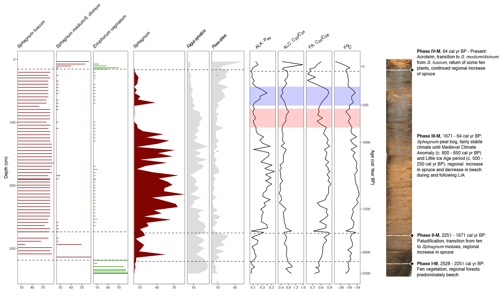
Figure 8Selected proxy curves from the macrofossil record (horizontal bars: S. fuscum, S. medium/divinum, E. vaginatum), pollen record (filled-in lines: Sphagnum, F. sylvatica, P. abies), and the biomarker and elemental records (lines; n-alkane Paq, n-alcohol , n-fatty acid , and δ13C). A composite photo of the core is also shown with the phases from the CONISS analysis of the macrofossils briefly described. The estimated time frames of the MCA and LIA are highlighted on the biomarker and elemental curves in red and blue, respectively.
4.3 Added value of biomarker analysis
Both the biomarker and the macrofossil analyses are reflective of the local vegetation within the peatland, while the pollen analysis reflects both the local and the regional vegetation. Timing differences between local and regional vegetation shifts have previously been reported in studies using biomarkers and pollen analyses (e.g., Jansen et al., 2013).
Despite potential discrepancies in the cluster-analysis-derived phases, the biomarker results illustrate a similar story of peatland development. The primary driver behind the phase changes in the biomarker data appeared to be the abundance of C25 n-alkane. As C25, along with C23, is known to be highly abundant in Sphagnum species, the phases resulting from the CONISS analysis most likely represent changes in the input of Sphagnum to the peat (Fig. 6). Comparing the biomarker results with those of the macrofossils and pollen, the increase in Sphagnum did generally correlate well (Figs. 4, 5, 6, 8). Moreover, the increase in Sphagnum and related biomarkers was paralleled by higher ratios and enriched δ13C values (Fig. 3), indicative of more ombrotrophic conditions (Wang et al., 2015). The n-alkanol ratio and the n-fatty-acid ratio also roughly followed these trends. While they have not previously been linked to Sphagnum mosses as indicative ratios, future peat biomarker studies could investigate this further.
One notable difference shown in the biomarker measurements as opposed to the macrofossils was the behavior of Paq, Pwax, and , as well as the n-alkanol ratio and the n-fatty-acid ratio in Phase III-B (Fig. 7). The generally decreasing trend in Paq and at the beginning of this phase implies lower water table levels and drier conditions, which could be related to the warmer Medieval Climate Anomaly (MCA; ca. 900–1400 CE) (Luterbacher et al., 2016). Then from around 500 to 345 cal yr BP, Paq began to increase, while Pwax decreased. This shift in conditions is also reflected in the δ13C values (Fig. 8) and in an abrupt increase in Sphagnum in the pollen data but is not reflected in a notable change in the macrofossils.
Additionally, all of the ACL measures reach a minimum at this same interval (Fig. 6), indicating a higher input of the shorter-chain-length homologues, which would also correspond with less input from vascular plants. Furthermore, the ratio reached a minimum in this interval, indicating a potential shift in Sphagnum species (McClymont et al., 2008). Following this brief increase, the Paq decreased again, while the Pwax increased until Phase IV-B or 35 cal yr BP (Fig. 7). This is likely linked to the increased human activity and drainage that occurred at the peatland in the 19th and 20th centuries (Swindles et al., 2019). The indication of Paq, Pwax, and of a change in local conditions that are not reflected in the macrofossils shows that biomarkers can be a valuable additional proxy to use in paleoenvironmental studies.
4.4 Comparison with other local and regional records
The developmental trajectory of the Beerberg peatland was similar to other peat bogs in Germany and other parts of central and northern Europe. The fen-to-bog transition occurred around 2250 cal yr BP, which has been recognized as the beginning of a shift to cooler and/or wetter periods in previous studies in Ireland (Barber et al., 2003), England (Wimble, 1986), and Denmark (Aaby, 1976). The next major transition seen in the core record was the Medieval Climate Anomaly (MCA) and Little Ice Age (LIA), the exact time of which varies across European paleoclimate records (Wanner et al., 2022). Here at the Beerberg peatland, we found evidence of warming in the biomarker measurements and the pollen record during the period ca. 1150–1300 CE, as shown by the decrease in Sphagnum in the pollen record as well as corresponding changes in the biomarker ratios. This was followed by a period of likely cooling from ca. 1450–1700 CE, shown by the return of Sphagnum in the pollen record and corresponding fluctuations in the biomarker ratios. We believe that these periods correspond to the MCA and LIA. This roughly overlaps with results from previous studies: for example, Mauquoy et al. (2002) identified the LIA as lasting from ca. 1450–1600 CE at Lille Vildmose in Denmark and ca. 1460–1600 CE at Walton Moss in England, Barber et al. (2004) identified the LIA as starting between ca. 1250–1350 CE at Dosenmoor in Germany and Svanemose in Denmark, and De Vleeschouwer et al. (2009) found evidence of the LIA from ca. 1200–1800 CE. Following the LIA, the Beerberg pollen record showed that the forests of the region transitioned from primarily F. sylvatica forests to P. abies forests, with an increase in P. sylvestris in the last few centuries as well. This pattern has been seen in many other northern and central European forests (e.g., Svobodová et al., 2002). The final vegetation transition at Beerberg beginning in the late 19th century, with an increase in Ericaceae species and E. vaginatum as well as a shift in dominant Sphagnum species, is likely related at least partially to human influence such as drainage of the peatlands and change in forest composition in the catchment. This has also been noted in other European records (Barber et al., 2004). Generally, the development of the Beerberg peatland confirmed patterns seen at other European sites, though locally transitions occurred with some offsets because of the exposed location of the sequence at the mountain ridge. As such offsets have been well documented, this shows that studying local archives are the most informative of local climate and environmental shifts. To the best of our knowledge, this study is the first of its kind covering the last 2 millennia in a peatland in central Germany, and its location in Thuringia enables future application to research identifying climate boundary shifts in central Europe (Breitenbach et al., 2019).
We found that the peatland itself, with Sphagnum fuscum as the dominant peat-forming species, did not undergo much vegetational change following its initial development. This stability persisted even amidst notable shifts in forest composition, from being beech- to spruce-dominated, and increased anthropogenic land use within the region. In the last couple of centuries, the pristine plant population of the peatland was disturbed, most likely by dust deposition and hydrological changes, as we were able to glean from the elemental and biomarker analyses despite the relative homogeneity of the macrofossil analysis.
This study has further demonstrated opportunities for biomarker analysis to contribute meaningfully to paleoenvironmental investigations. Specifically, the biomarker record serves as an independent confirmation of the trends found in the pollen and macrofossils, providing more confidence in the vegetation reconstruction, especially on a species level. The n-alkane ratios provided more precise information about fluctuations in the local conditions of the peat bog, pointing to potential influences from regional climate shifts that underpin the observed changes in vegetation from the pollen and macrofossil data. We also identified two more potential diagnostic biomarker ratios for Sphagnum abundance: the n-alkanol and n-fatty acid . Additionally, the fact that multiple parameters, such as various sources of organic matter and processes like degradation and preservation of organic matter, can be assessed confirms the high potential for biomarker applications in peat records. However, the numerous molecular proxies derived from biomarker composition are often difficult to interpret independently, requiring certain expertise and the assessment of biomarkers from several compound classes to gain supportive data for certain interpretations.
Consequently, to increase the effectiveness and efficiency of biomarker analyses, a more systematic approach is required, aiming at integrating biomarker compound classes more holistically. The vast majority of biomarker indices and ratios have been developed for n-alkanes, neglecting other compounds such as n-fatty acids and n-alkanols. While the n-alkanes were the most useful compound class for our study, it would be beneficial if other compounds and potential diagnostic ratios were investigated and applied more systematically, as we have done here.
Radiocarbon dates
Table A1Radiocarbon dates of selected organic remains. The sample from a depth of 7.5 cm was excluded from the age–depth model.
All data are available at Pangaea via https://doi.org/10.1594/PANGAEA.961142 (Thomas et al., 2023).
CLT: conceptualization, formal analysis, investigation, data curation, writing (original draft as well as review and editing), visualization; BJ: writing (review and editing), supervision; SC: formal analysis, investigation, writing (review and editing), visualization; MG: methodology, formal analysis, investigation, writing (review and editing), visualization; KHK: conceptualization, methodology, writing (review and editing); EEvL: writing (review and editing), supervision; ME: formal analysis, investigation, writing (review and editing); GLBW: conceptualization, methodology, resources, writing (review and editing), supervision, project administration, funding acquisition.
The contact author has declared that none of the authors has any competing interests.
Publisher's note: Copernicus Publications remains neutral with regard to jurisdictional claims made in the text, published maps, institutional affiliations, or any other geographical representation in this paper. While Copernicus Publications makes every effort to include appropriate place names, the final responsibility lies with the authors.
We are grateful for funding from swissuniversities in the form of a grant supporting the cotutelle de thèse project of CLT. We thank the Vessertal–Thuringian Forest Biosphere Reserve for allowing us to sample, as well as Marcin Kiedrzyński for his assistance during fieldwork. We are grateful to Thomy Keller for his assistance in obtaining radiocarbon dates. Additional laboratory support was provided by Yves Brügger, Aline Hobi, Tatjana Kraut, Barbara Siegfried, and Dmitry Tikhomirov. Carrie L. Thomas thanks Tiia Määttä for her helpful comments and insight into peatlands.
This research has been supported by the Swiss National Science Foundation (grant no. 188684).
This paper was edited by Petr Kuneš and reviewed by two anonymous referees.
Aaby, B.: Cyclic climatic variations in climate over the past 5,500 yr reflected in raised bogs, Nature, 263, 281–284, https://doi.org/10.1038/263281a0 1976. a
Ackerman, D., Millet, D. B., and Chen, X.: Global estimates of inorganic nitrogen deposition across four decades, Global Biogeochem. Cy., 33, 100–107, https://doi.org/10.1029/2018GB005990 2019. a
Andersson, R. A., Kuhry, P., Meyers, P. A., Zebühr, Y., Crill, P., and Mörth, M.: Impacts of paleohydrological changes on n-alkane biomarker compositions of a Holocene peat sequence in the eastern European Russian Arctic, Org. Geochem., 42, 1065–1075, https://doi.org/10.1016/j.orggeochem.2011.06.020, 2011. a, b
Baas, M., Pancost, R. D., van Geel, B., and Damsté, J. S. S.: A comparative study of lipids in Sphagnum species, Org. Geochem., 31, 535–541, https://doi.org/10.1016/S0146-6380(00)00037-1, 2000. a, b
Balascio, N. L., Anderson, R. S., D'Andrea, W. J., Wickler, S., D'Andrea, R. M., and Bakke, J.: Vegetation changes and plant wax biomarkers from an ombrotrophic bog define hydroclimate trends and human-environment interactions during the Holocene in northern Norway, Holocene, 30, 1849–1865, https://doi.org/10.1177/0959683620950456, 2020. a
Barber, K. E., Chambers, F. M., Maddy, D., Stoneman, R., and Brew, J. S.: A sensitive high-resolution record of late Holocene climatic change from a raised bog in northern England, Holocene, 4, 198–205, https://doi.org/10.1177/095968369400400209, 1994. a
Barber, K. E., Chambers, F. M., and Maddy, D.: Holocene palaeoclimates from peat stratigraphy: macrofossil proxy climate records from three oceanic raised bogs in England and Ireland, Quaternary Sci. Rev., 22, 521–539, https://doi.org/10.1016/S0277-3791(02)00185-3 2003. a
Barber, K. E., Chambers, F. M., and Maddy, D.: Late Holocene climatic history of northern Germany and Denmark: peat macrofossil investigations at Dosenmoor, Schleswig-Holstein, and Svanemose, Jutland, Boreas, 33, 132–144, https://doi.org/10.1111/j.1502-3885.2004.tb01135.x 2004. a, b, c
Behre, K. E.: Interpretation of anthropogenic indicators in pollen diagrams, Pollen et Spores, 23, 225–245, 1981. a
Bennett, K. D.: Determination of the number of zones in a biostratigraphical sequence, New Phytol., 132, 155–170, https://doi.org/10.1111/j.1469-8137.1996.tb04521.x, 1996. a
Berglund, B. E. and Ralska-Jasiewiczowa, M.: Pollen analysis and pollen diagrams, in: Handbook of Holocene Palaeoecology and Palaeohydrology, edited by: Berglund, B. E., pp. 455–484, John Wiley & Sons, Chichester, 1986. a
Beug, H. J.: Leitfaden der Pollenbestimmung für Mitteleuropa und angrenzende Gebiete, G. Fischer, 1961. a
Biester, H., Knorr, K.-H., Schellekens, J., Basler, A., and Hermanns, Y.-M.: Comparison of different methods to determine the degree of peat decomposition in peat bogs, Biogeosciences, 11, 2691–2707, https://doi.org/10.5194/bg-11-2691-2014, 2014. a, b, c
Bingham, E. M., McClymont, E. L., Väliranta, M., Mauquoy, D., Roberts, Z., Chambers, F. M., Pancost, R. D., and Evershed, R. P.: Conservative composition of n-alkane biomarkers in Sphagnum species: implications for palaeoclimate reconstruction in ombrotrophic peat bogs, Org. Geochem., 41, 214–220, https://doi.org/10.1016/j.orggeochem.2009.06.010, 2010. a
Birks, H. H. and Birks, H. J. B.: Future uses of pollen analysis must include plant macrofossils, J. Biogeogr., 27, 31–35, https://www.jstor.org/stable/2655981 (last access: 20 March 2023), 2000. a, b, c, d
Blaauw, M. and Christen, J. A.: Flexible paleoclimate age-depth models using an autoregressive gamma process, Bayesian Anal., 6, 457 – 474, https://doi.org/10.1214/11-BA618 2011. a, b
Blaauw, M., Christen, J. A., and Aquino López, M. A.: rbacon: Age-Depth Modelling using Bayesian Statistics, https://CRAN.R-project.org/package=rbacon (last access: 15 March 2021), R package version 2.5.2, 2021. a
Breitenbach, S. F., Plessen, B., Waltgenbach, S., Tjallingii, R., Leonhardt, J., Jochum, K. P., Meyer, H., Goswami, B., Marwan, N., and Scholz, D.: Holocene interaction of maritime and continental climate in Central Europe: New speleothem evidence from Central Germany, Global Planet. Change, 176, 144–161, https://doi.org/10.1016/j.gloplacha.2019.03.007 2019. a, b, c
Chambers, F. M., Booth, R. K., De Vleeschouwer, F., Lamentowicz, M., Le Roux, G., Mauquoy, D., Nichols, J. E., and Van Geel, B.: Development and refinement of proxy-climate indicators from peats, Quatern. Int., 268, 21–33, https://doi.org/10.1016/j.quaint.2011.04.039, 2012. a, b, c, d, e
Chibnall, A. C., Piper, S. H., Pollard, A., Williams, E. F., and Sahai, P. N.: The constitution of the primary alcohols, fatty acids and paraffins present in plant and insect waxes, Biochem. J., 28, 2189, https://doi.org/10.1042/bj0282189, 1934. a
Corrigan, D., Kxoos, M., O'Connor, C., and Timoney, R.: LIPID COMPONENTS OF SPHAGNUM MOSSES, Planta Med., 29, 261–267, https://doi.org/10.1055/s-0028-1097660 1976. a
Czerwiński, S., Margielewski, W., Gałka, M., and Kołaczek, P.: Late Holocene transformations of lower montane forest in the Beskid Wyspowy Mountains (Western Carpathians, Central Europe): a case study from Mount Mogielica, Palynology, 44, 355–368, https://doi.org/10.1080/01916122.2019.1617207, 2020. a
Davis, M. B. and Deevey, E. S.: Pollen accumulation rates: Estimates from Late-Glacial sediment of Rogers Lake, Science, 145, 1293–1295, https://doi.org/10.1126/science.145.3638.1293 1964. a
De Vleeschouwer, F., Piotrowska, N., Sikorski, J., Pawlyta, J., Cheburkin, A., Le Roux, G., Lamentowicz, M., Fagel, N., and Mauquoy, D.: Multiproxy evidence of `Little Ice Age' palaeoenvironmental changes in a peat bog from northern Poland, Holocene, 19, 625–637, https://doi.org/10.1177/0959683609104027 2009. a
Eglinton, G. and Hamilton, R. J.: Leaf epicuticular waxes: The waxy outer surfaces of most plants display a wide diversity of fine structure and chemical constituents, Science, 156, 1322–1335, https://doi.org/10.1126/science.156.3780.1322, 1967. a
Farrimond, P. and Flanagan, R. L.: Lipid stratigraphy of a Flandrian peat bed (Northumberland, UK): comparison with the pollen record, Holocene, 6, 69–74, https://doi.org/10.1177/095968369600600108, 1996. a, b
Ficken, K. J., Barber, K. E., and Eglinton, G.: Lipid biomarker, δ13C and plant macrofossil stratigraphy of a Scottish montane peat bog over the last two millennia, Org. Geochem., 28, 217–237, https://doi.org/10.1016/S0146-6380(97)00126-5, 1998a. a, b, c
Ficken, K. J., Street-Perrott, F. A., Perrott, R. A., Swain, D. L., Olago, D. O., and Eglinton, G.: Glacial/interglacial variations in carbon cycling revealed by molecular and isotope stratigraphy of Lake Nkunga, Mt. Kenya, East Africa, Org. Geochem., 29, 1701–1719, https://doi.org/10.1016/S0146-6380(98)00109-0, 1998b. a
Ficken, K. J., Li, B., Swain, D. L., and Eglinton, G.: An n-alkane proxy for the sedimentary input of submerged/floating freshwater aquatic macrophytes, Org. Geochem., 31, 745–749, https://doi.org/10.1016/S0146-6380(00)00081-4, 2000. a
Finsinger, W. and Tinner, W.: Minimum count sums for charcoal concentration estimates in pollen slides: Accuracy and potential errors, Holocene, 15, 293–297, https://doi.org/10.1191/0959683605hl808rr, 2005. a
Gaillard, M.-J.: Archaeological applications, in: The Encyclopedia of Quaternary Science, pp. 880–904, Elsevier, 2013. a
Gałka, M., Szal, M., Broder, T., Loisel, J., and Knorr, K.-H.: Peatbog resilience to pollution and climate change over the past 2700 years in the Harz Mountains, Germany, Ecol. Indic., 97, 183–193, https://doi.org/10.1016/j.ecolind.2018.10.015, 2019. a, b
Gałka, M., Diaconu, A.-C., Feurdean, A., Loisel, J., Teickner, H., Broder, T., and Knorr, K.-H.: Relations of fire, palaeohydrology, vegetation succession, and carbon accumulation, as reconstructed from a mountain bog in the Harz Mountains (Germany) during the last 6200 years, Geoderma, 424, 115991, https://doi.org/10.1016/j.geoderma.2022.115991, 2022a. a
Gałka, M., Hölzer, A., Feurdean, A., Loisel, J., Teickner, H., Diaconu, A.-C., Szal, M., Broder, T., and Knorr, K.-H.: Insight into the factors of mountain bog and forest development in the Schwarzwald Mts.: Implications for ecological restoration, Ecol. Indic., 140, 109039, https://doi.org/10.1016/j.ecolind.2022.109039, 2022b. a, b, c
Githumbi, E., Fyfe, R., Gaillard, M.-J., Trondman, A.-K., Mazier, F., Nielsen, A.-B., Poska, A., Sugita, S., Woodbridge, J., Azuara, J., Feurdean, A., Grindean, R., Lebreton, V., Marquer, L., Nebout-Combourieu, N., Stančikaitė, M., Tanţău, I., Tonkov, S., Shumilovskikh, L., and LandClimII data contributors: European pollen-based REVEALS land-cover reconstructions for the Holocene: methodology, mapping and potentials, Earth Syst. Sci. Data, 14, 1581–1619, https://doi.org/10.5194/essd-14-1581-2022, 2022. a
Görner, M., Haupt, R., Hiekel, W., Niemann, E., and Westhus, W.: Die Naturschutzgebiete der Bezirke Erfurt, Suhl und Gera, in: Handbuch der Naturschutzgebiete der Deutschen Demokratischen Republik, Bd. 4, edited by: Weinitschke, H., Urania-Verlag, Leipzig, Jena, Berlin, pp. 99–101, 1984. a
Grimm, E. C.: CONISS: a FORTRAN 77 program for stratigraphically constrained cluster analysis by the method of incremental sum of squares, Comput. Geosci., 13, 13–35, https://doi.org/10.1016/0098-3004(87)90022-7, 1987. a, b, c
Grimm, E. C.: TILIA 2.0 Pollen Analysis Software, https://www.neotomadb.org/apps/tilia (last access: 9 December 2023), 1993. a
Hepp, J., Wüthrich, L., Bromm, T., Bliedtner, M., Schäfer, I. K., Glaser, B., Rozanski, K., Sirocko, F., Zech, R., and Zech, M.: How dry was the Younger Dryas? Evidence from a coupled –δ18O biomarker paleohygrometer applied to the Gemündener Maar sediments, Western Eifel, Germany, Clim. Past, 15, 713–733, https://doi.org/10.5194/cp-15-713-2019, 2019. a
Hölzer, A.: Die Torfmoose: Südwestdeutschlands und der Nachbargebiete, Weissdorn Verlag, 2010. a, b
Hua, Q., Barbetti, M., and Rakowski, A. Z.: Atmospheric radiocarbon for the period 1950–2010, Radiocarbon, 55, 2059–2072, https://doi.org/10.2458/azu_js_rc.v55i2.16177, 2013. a
Jahn, R.: Pollenanalytische Untersuchungen an Hochmooren des Thüringer Waldes, Forstwiss. Centralbl., 52, 761–774, 1930. a, b
Jansen, B. and Wiesenberg, G. L. B.: Opportunities and limitations related to the application of plant-derived lipid molecular proxies in soil science, SOIL, 3, 211–234, https://doi.org/10.5194/soil-3-211-2017, 2017. a, b, c
Jansen, B., de Boer, E. J., Cleef, A. M., Hooghiemstra, H., Moscol-Olivera, M., Tonneijck, F. H., and Verstraten, J. M.: Reconstruction of late Holocene forest dynamics in northern Ecuador from biomarkers and pollen in soil cores, Palaeogeogr Palaeocl., 386, 607–619, https://doi.org/10.1016/j.palaeo.2013.06.027 2013. a
Jeschke, L. and Paulson, C.: Pflege-und Entwicklungspläne für die Hochmoore in den Kammlagen des Thüringer Waldes, Beerbergmoor, Saukopfmoor, Schneekopfmoore und Schützenbergmoor, unter Mitarbeit von Ch. Paulson und der Geocad-Ingenieurgesellschaft mbH, unveröffentlichtes Gutachten im Auftrag des Staatlichen Umweltamtes Erfurt, 2000. a
Jones, M. C., Peteet, D. M., and Sambrotto, R.: Late-glacial and Holocene δ15N and δ13C variation from a Kenai Peninsula, Alaska peatland, Palaeogeogr Palaeocl., 293, 132–143, https://doi.org/10.1016/j.palaeo.2010.05.007, 2010. a
Juggins, S.: rioja: Analysis of Quaternary Science Data, CRAN [code], https://cran.r-project.org/package=rioja (last access: 5 September 2023), R package version 0.9-26, 2022. a
Karpińska-Kołaczek, M., Kołaczek, P., and Stachowicz-Rybka, R.: Pathways of woodland succession under low human impact during the last 13,000 years in northeastern Poland, Quatern. Int., 328, 196–212, https://doi.org/10.1016/j.quaint.2013.11.038, 2014. a
Kołaczek, P., Margielewski, W., Gałka, M., Karpińska-Kołaczek, M., Buczek, K., Lamentowicz, M., Borek, A., Zernitskaya, V., and Marcisz, K.: Towards the understanding the impact of fire on the lower montane forest in the Polish Western Carpathians during the Holocene, Quaternary Sci. Rev., 229, 106137, https://doi.org/10.1016/j.quascirev.2019.106137, 2020. a, b
Kuhry, P. and Vitt, D. H.: Fossil carbon/nitrogen ratios as a measure of peat decomposition, Ecology, 77, 271–275, https://doi.org/10.2307/2265676, 1996. a, b, c, d
Kuhry, P., Halsey, L., Bayley, S., and Vitt, D.: Peatland development in relation to Holocene climatic change in Manitoba and Saskatchewan (Canada), Can. J. Earth Sci., 29, 1070–1090, https://doi.org/10.1139/e92-086, 1992. a, b
Laine, J., Flatberg, K. I., Harju, P., Timonen, T., Minkkinen, K. J., Laine, A., Tuittila, E.-S., and Vasander, H. T.: Sphagnum mosses: the stars of European mires, Sphagna Ky., 2018. a
Lange, E.: Zur Vegetationsgeschichte des Beerberggebietes im Thüringer Wald, Feddes Repertorium, 76, 205–219, 1967. a, b
Latałowa, M., Pędziszewska, A., Maciejewska, E., and Święta-Musznicka, J.: Tilia forest dynamics, Kretzschmaria deusta attack, and mire hydrology as palaeoecological proxies for mid-Holocene climate reconstruction in the Kashubian Lake District (N Poland), Holocene, 23, 667–677, https://doi.org/10.1177/0959683612467484, 2013. a
Loisel, J., Garneau, M., and Hélie, J.-F.: Sphagnum δ13C values as indicators of palaeohydrological changes in a peat bog, Holocene, 20, 285–291, 2010. a, b, c, d, e
Luterbacher, J., Werner, J. P., Smerdon, J. E., Fernández-Donado, L., González-Rouco, F. J., Barriopedro, D., Ljungqvist, F. C., Büntgen, U., Zorita, E., Wagner, S., Esper, J., McCarroll, D., Toreti, A., Frank, D., Jungclaus, J. H., Barriendos, M., Bertolin, C., Bothe, O., Brázdil, R., Camuffo, D., Dobrovolný, P., Gagen, M., García-Bustamante, E., Ge, Q., Gómez-Navarro, J. J., Guiot, J., Hao, Z., Hegerl, G. C., Holmgren, K., Klimenko, V. V., Martín-Chivelet, J., Pfister, C., Roberts, N., Schindler, A., Schurer, A., Solomina, O., von Gunten, L., Wahl, E., Wanner, H., Wetter, O., Xoplaki, E., Yuan, N., Zanchettin, D., Zhang, H., and Zerefos, C.: European summer temperatures since Roman times, Environ. Res. Lett., 11, 024001, https://doi.org/10.1088/1748-9326/11/2/024001 2016. a, b
Lützner, H., Andreas, D., Schneider, J. W., Voigt, S., and Werneburg, R.: Stefan und Rotliegend im Thüringer Wald und seiner Umgebung, Deutsche Stratigraphische Kommission: Subkommission Perm-Trias, Stratigraphie von Deutschland X, Rotliegend, Teil I: Innervariscische Becken, Schriftenreihe der Deutschen Gesellschaft für Geowissenschaften, 61, 418–487, 2012. a
MacArthur, R. H.: On the relative abundance of bird species, P. Natl. Acad. Sci. USA, 43, 293–295, https://doi.org/10.1073/pnas.43.3.293, 1957. a
Marcisz, K., Kołaczek, P., Gałka, M., Diaconu, A.-C., and Lamentowicz, M.: Exceptional hydrological stability of a Sphagnum-dominated peatland over the late Holocene, Quaternary Sci. Rev., 231, 106180, https://doi.org/10.1016/j.quascirev.2020.106180 2020. a
Marzi, R., Torkelson, B., and Olson, R.: A revised carbon preference index, Org. Geochem., 20, 1303–1306, https://doi.org/10.1016/0146-6380(93)90016-5 1993. a
Mauquoy, D. and Van Geel, B.: Plant macrofossil methods and studies: mire and peat macros, in: Encyclopedia of Quaternary Science, pp. 2315–2336, Elsevier Science, 2007. a
Mauquoy, D., Van Geel, B., Blaauw, M., and Van Der Plicht, J.: Evidence from northwest European bogs shows ‘Little Ice Age' climatic changes driven by variations in solar activity, Holocene, 12, 1–6, https://doi.org/10.1191/0959683602hl514rr 2002. a
McClymont, E. L., Mauquoy, D., Yeloff, D., Broekens, P., Van Geel, B., Charman, D. J., Pancost, R. D., Chambers, F. M., and Evershed, R. P.: The disappearance of Sphagnum imbricatum from Butterburn Flow, UK, Holocene, 18, 991–1002, https://doi.org/10.1177/0959683608093537, 2008. a, b
Moore, P. D., Webb, J. A., and Collison, M. E.: Pollen Analysis, Blackwell Scientific Publications, 1991. a
Naafs, B. D. A., Inglis, G. N., Blewett, J., McClymont, E. L., Lauretano, V., Xie, S., Evershed, R. P., and Pancost, R. D.: The potential of biomarker proxies to trace climate, vegetation, and biogeochemical processes in peat: A review, Global Planet. Change, 179, 57–79, https://doi.org/10.1016/j.gloplacha.2019.05.006, 2019. a, b
Nichols, J. E., Booth, R. K., Jackson, S. T., Pendall, E. G., and Huang, Y.: Paleohydrologic reconstruction based on n-alkane distributions in ombrotrophic peat, Org. Geochem., 37, 1505–1513, https://doi.org/10.1016/j.orggeochem.2006.06.020, 2006. a
Oksanen, J., Blanchet, F. G., Friendly, M., Kindt, R., Legendre, P., McGlinn, D., Minchin, P. R., O'Hara, R. B., Simpson, G. L., Solymos, P., Stevens, M. H. H., Szoecs, E., and Wagner, H.: vegan: Community Ecology Package, CRAN [code], https://CRAN.R-project.org/package=vegan (last access: 5 September 2023), R package version 2.5-7, 2022. a
Pancost, R. D., Baas, M., van Geel, B., and Damsté, J. S. S.: Biomarkers as proxies for plant inputs to peats: an example from a sub-boreal ombrotrophic bog, Org. Geochem., 33, 675–690, https://doi.org/10.1016/S0146-6380(02)00048-7, 2002. a, b, c, d
Peel, M. C., Finlayson, B. L., and McMahon, T. A.: Updated world map of the Köppen-Geiger climate classification, Hydrol. Earth Syst. Sci., 11, 1633–1644, https://doi.org/10.5194/hess-11-1633-2007, 2007. a
Poynter, J. G., Farrimond, P., Robinson, N., and Eglinton, G.: Aeolian-Derived Higher Plant Lipids in the Marine Sedimentary Record: Links with Palaeoclimate, in: Paleoclimatology and Paleometeorology: Modern and Past Patterns of Global Atmospheric Transport, edited by: Leinen, M. and Sarnthein, M., Springer Netherlands, Dordrecht, https://doi.org/10.1007/978-94-009-0995-3_18, pp. 435–462, 1989. a
R Core Team: R: A Language and Environment for Statistical Computing, R Foundation for Statistical Computing, Vienna, Austria, CRAN [code], https://www.R-project.org/ (last access: 20 March 2023), 2023. a
Reimer, P. J., Austin, W. E. N., Bard, E., Bayliss, A., Blackwell, P. G., Bronk Ramsey, C., Butzin, M., Cheng, H., Edwards, R. L., Friedrich, M., Grootes, P. M., Guilderson, T. P., Hajdas, I., Heaton, T. J., Hogg, A. G., Hughen, K. A., Kromer, B., Manning, S. W., Muscheler, R., Palmer, J. G., Pearson, C., van der Plicht, J., Reimer, R. W., Richards, D. A., Scott, E. M., Southon, J. R., Turney, C. S. M., Wacker, L., Adolphi, F., Büntgen, U., Capano, M., Fahrni, S. M., Fogtmann-Schulz, A., Friedrich, R., Köhler, P., Kudsk, S., Miyake, F., Olsen, J., Reinig, F., Sakamoto, M., Sookdeo, A., and Talamo, S.: The IntCal20 Northern Hemisphere radiocarbon age calibration curve (0–55 cal kBP), Radiocarbon, 62, 725–757, https://doi.org/10.1017/RDC.2020.41, 2020. a
Ronkainen, T., McClymont, E. L., Väliranta, M., and Tuittila, E.-S.: The n-alkane and sterol composition of living fen plants as a potential tool for palaeoecological studies, Org. Geochem., 59, 1–9, https://doi.org/10.1016/j.orggeochem.2013.03.005 2013. a
Ronkainen, T., Väliranta, M., McClymont, E. L., Biasi, C., Salonen, S., Fontana, S., and Tuittila, E.-S.: A combined biogeochemical and palaeobotanical approach to study permafrost environments and past dynamics, J. Quaternary Sci., 30, 189–200, https://doi.org/10.1002/jqs.2763, 2015. a
Rösch, M.: Long-term human impact as registered in an upland pollen profile from the southern Black Forest, south-western Germany, Veg. Hist. Archaeobot., 9, 205–218, https://doi.org/10.1007/BF01294635, 2000. a
Schwark, L., Zink, K., and Lechterbeck, J.: Reconstruction of postglacial to early Holocene vegetation history in terrestrial Central Europe via cuticular lipid biomarkers and pollen records from lake sediments, Geology, 30, 463–466, https://doi.org/10.1130/0091-7613(2002)030<0463:ROPTEH>2.0.CO;2, 2002. a, b
Shumilovskikh, L. S. and van Geel, B.: Non-Pollen Palynomorphs, in: Handbook for the Analysis of Micro-Particles in Archaeological Samples, edited by: Henry, A. G., Springer International Publishing, Cham, https://doi.org/10.1007/978-3-030-42622-4_4, pp. 65–94, 2020. a
Sim, T. G., Swindles, G. T., Morris, P. J., Baird, A. J., Cooper, C. L., Gallego-Sala, A. V., Charman, D. J., Roland, T. P., Borken, W., Mullan, D. J., Aquino-López, M. A., and Gałka, M.: Divergent responses of permafrost peatlands to recent climate change, Environ. Res. Lett., 16, 034001, https://doi.org/10.1088/1748-9326/abe00b 2021. a
Smith, A. J. E.: The moss flora of Britain and Ireland, Cambridge University Press, 2004. a
Speranza, A., Hanke, J., van Geel, B., and Fanta, J.: Late-Holocene human impact and peat development in the Černá Hora bog, Krkonoše Mountains, Czech Republic, Holocene, 10, 575–585, https://doi.org/10.1191/095968300668946885, 2000. a, b
Stivrins, N., Ozola, I., Gałka, M., Kuske, E., Alliksaar, T., Andersen, T. J., Lamentowicz, M., Wulf, S., and Reitalu, T.: Drivers of peat accumulation rate in a raised bog: Impact of drainage, climate, and local vegetation composition, Mires Peat, 19, 1–19, https://doi.org/10.19189/MaP.2016.OMB.262, 2017. a
Stivrins, N., Aakala, T., Ilvonen, L., Pasanen, L., Kuuluvainen, T., Vasander, H., Gałka, M., Disbrey, H. R., Liepins, J., Holmström, L., and Seppä, H.: Integrating fire-scar, charcoal and fungal spore data to study fire events in the boreal forest of northern Europe, Holocene, 29, 1480–1490, https://doi.org/10.1177/0959683619854524, 2019. a
Stockmarr, J.: Tablets with spores used in absolute pollen analysis, Pollen et Spores, 13, 615–621, 1971. a
Svobodová, H., Soukupová, L., and Reille, M.: Diversified development of mountain mires, Bohemian Forest, Central Europe, in the last 13,000 years, Quatern. Int., 91, 123–135, https://doi.org/10.1016/S1040-6182(01)00106-9 2002. a
Swindles, G. T., Morris, P. J., Mullan, D. J., Payne, R. J., Roland, T. P., Amesbury, M. J., Lamentowicz, M., Turner, T. E., Gallego-Sala, A., Sim, T., Barr, I. D., Blaauw, M., Blundell, A., Chambers, F. M., Charman, D. J., Feurdean, A., Galloway, J. M., Gałka, M., Green, S. M., Kajukało, K., Karofeld, E., Korhola, A., Lamentowicz, Ł, Langdon, P., Marcisz, K., Mauquoy, D., Mazei, Y. A., McKeown, M. M., Mitchell, E. A. D., Novenko, E., Plunkett, G., Roe, H. M., Schoning, K., Sillasoo, Ü, Tsyganov, A. N., van der Linden, M., Väliranta, M., and Warner, B.: Widespread drying of European peatlands in recent centuries, Nature Geoscience, 12, 922–928, https://doi.org/10.1038/s41561-019-0462-z, 2019. a, b, c
Thüringer Landesanstalt für Umwelt und Geologie: Moore in den Kammlagen des Thüringer Waldes, 2002. a
Tinner, W. and Hu, F. S.: Size parameters, size-class distribution and area-number relationship of microscopic charcoal: relevance for fire reconstruction, Holocene, 13, 499–505, https://doi.org/10.1191/0959683603hl615rp, 2003. a
Tinner, W., Conedera, M., Gobet, E., Hubschmid, P., Wehrli, M., and Ammann, B.: A palaeoecological attempt to classify fire sensitivity of trees in the southern Alps, Holocene, 10, 565–574, https://doi.org/10.1191/095968300674242447, 2000. a
Thomas, C. L., Jansen, B., Czerwiński, S., Gałka, M., Knorr, K.-H., van Loon, E. E., Egli, M., and Wiesenberg, G. L. B.: Paleobotanical and biomarker records over 2600 years from Beerberg peatland (Central Germany), PANGAEA [data set], https://doi.org/10.1594/PANGAEA.961142, 2023. a
Tuittila, E.-S., Väliranta, M., Laine, J., and Korhola, A.: Quantifying patterns and controls of mire vegetation succession in a southern boreal bog in Finland using partial ordinations, J. Veg. Sci., 18, 891–902, https://www.jstor.org/stable/4499301, 2007. a, b
Von Post, L.: Forest tree pollen in south Swedish peat bog deposits, translated: Davis, M. B. and Faegri, K. (1967), Pollen et Spores, 9, 375–401, 1916. a
Wang, M., Moore, T. R., Talbot, J., and Riley, J. L.: The stoichiometry of carbon and nutrients in peat formation, Global Biogeochem. Cy., 29, 113–121, https://doi.org/10.1002/2014GB005000, 2015. a, b
Wanner, H., Pfister, C., and Neukom, R.: The variable European Little Ice Age, Quaternary Sci. Rev., 287, 107531, https://doi.org/10.1016/j.quascirev.2022.107531 2022. a
Wiesenberg, G. L. B. and Gocke, M. I.: Analysis of lipids and polycyclic aromatic hydrocarbons as indicators of past and present (micro)biological activity, in: Hydrocarbon and Lipid Microbiology Protocols: Petroleum, Hydrocarbon and Lipid Analysis, edited by McGenity, T. J., Timmis, K. N., and Nogales, B., Springer Berlin Heidelberg, Berlin, Heidelberg, https://doi.org/10.1007/8623_2015_157, pp. 61–91, 2017. a
Wilkins, W.: Studies in the genus Ustulina–With special reference to parasitism: I. Introduction, survey of previous literature and host index, T. Brit. Mycol. Soc., 18, 320–346, https://doi.org/10.1016/S0007-1536(34)80017-4, 1934. a
Wimble, G.: The palaeoecology of the lowland coastal raised mires of South Cumbria, PhD thesis, University College, 1986. a
Xie, S., Nott, C. J., Avsejs, L. A., Maddy, D., Chambers, F. M., and Evershed, R. P.: Molecular and isotopic stratigraphy in an ombrotrophic mire for paleoclimate reconstruction, Geochim. Cosmochim. Ac., 68, 2849–2862, https://doi.org/10.1016/j.gca.2003.08.025, 2004. a, b
Xu, J., Morris, P. J., Liu, J., and Holden, J.: PEATMAP: Refining estimates of global peatland distribution based on a meta-analysis, Catena, 160, 134–140, https://doi.org/10.1016/j.catena.2017.09.010, 2018. a
Yu, Z., Loisel, J., Brosseau, D. P., Beilman, D. W., and Hunt, S. J.: Global peatland dynamics since the Last Glacial Maximum, Geophys. Res. Lett., 37, L13402, https://doi.org/10.1029/2010GL043584, 2010. a
Zheng, Y., Zhou, W., Meyers, P. A., and Xie, S.: Lipid biomarkers in the Zoigê-Hongyuan peat deposit: Indicators of Holocene climate changes in West China, Org. Geochem., 38, 1927–1940, https://doi.org/10.1016/j.orggeochem.2007.06.012, 2007. a, b, c
Zheng, Y., Zhou, W., Liu, Z., and Liu, X.: The n-alkanol paleoclimate records in two peat deposits: a comparative study of the northeastern margin of the Tibetan Plateau and Northeast China, Environ. Earth Sci., 63, 135–143, https://doi.org/10.1007/s12665-010-0676-2 2011. a
Zhou, W., Xie, S., Meyers, P. A., and Zheng, Y.: Reconstruction of late glacial and Holocene climate evolution in southern China from geolipids and pollen in the Dingnan peat sequence, Org. Geochem., 36, 1272–1284, https://doi.org/10.1016/j.epsl.2010.02.035, 2005. a, b