Identifying landscape hot and cold spots of soil greenhouse gas fluxes by combining field measurements and remote sensing data

Upscaling chamber measurements of soil greenhouse gas (GHG) fluxes from point scale to landscape scale remain challenging due to the high variability in the fluxes in space and time. This study measured GHG fluxes and soil parameters at selected point locations (n=268), thereby implementing a stratified sampling approach on a mixed-land-use landscape (∼5.8 km²). Based on these field-based measurements and remotely sensed data on landscape and vegetation properties, we used random forest (RF) models to predict GHG fluxes at a landscape scale (1 m resolution) in summer and autumn. The RF models, combining field-measured soil parameters and remotely sensed data, outperformed those with field-measured predictors or remotely sensed data alone. Available satellite data products from Sentinel-2 on vegetation cover and water content played a more significant role than those attributes derived from a digital elevation model, possibly due to their ability to capture both spatial and seasonal changes in the ecosystem parameters within the landscape. Similar seasonal patterns of higher soil/ecosystem respiration (SR/ER–CO₂) and nitrous oxide (N₂O) fluxes in summer and higher methane (CH₄) uptake in autumn were observed in both the measured and predicted landscape fluxes. Based on the upscaled fluxes, we also assessed the contribution of hot spots to the total landscape fluxes. The identified emission hot spots occupied a small landscape area (7 % to 16 %) but accounted for up to 42 % of the landscape GHG fluxes. Our study showed that combining remotely sensed data with chamber measurements and soil properties is a promising approach for identifying spatial patterns and hot spots of GHG fluxes across heterogeneous landscapes. Such information may be used to inform targeted mitigation strategies at the landscape scale.

1 Introduction

Atmospheric concentrations of greenhouse gases (GHGs) such as carbon dioxide (CO₂), methane (CH₄), and nitrous oxide (N₂O) have increased since the 1750s, substantially driving global climate change (IPCC, 2019). Soils are key contributors to these GHG fluxes, with recent global emissions of approximately 350 Pg CO₂ equivalent per year (Oertel et al., 2016). Soil GHG emissions have accelerated due to human activities such as land use change for agricultural land expansion (Dhakal et al., 2022). Globally, agricultural soils are significant sources, accounting for about 37 % of the GHG emissions within the agricultural sector (Tubiello et al., 2013). However, the estimates of soil GHG fluxes are highly uncertain, since soil properties, land use, and land management, which are key indirect drivers of the emissions, largely differ across landscapes and regions. For instance, global annual estimates range widely from 67 to 101 Pg C (Jian et al., 2018) for soil respiration, 2.5–6.5 Tg N₂O−N for annual soil N₂O emissions (Tian et al., 2020), and 12–60 Tg for soil-CH₄-uptake rates (Dutaur and Verchot, 2007). These uncertainties make it difficult to accurately quantify the GHG source or sink strengths of soils and to develop targeted mitigation options across scales.

Current upscaling approaches from localized measurements of soil GHG fluxes to landscape or regional scales, using chamber- or site-specific micro-meteorological methods such as eddy covariance (e.g., Sundqvist et al., 2015; Warner et al., 2019; Vainio et al., 2021; Han et al., 2022), fail to capture the spatiotemporal variation in the hot or cold spots, resulting in uncertainties in regional and global GHG estimates (Hagedorn and Bellamy, 2011; Levy et al., 2022). Contrary to the eddy covariance method, chamber-based approaches can be used to capture fine-scale spatial variabilities in the soil GHG fluxes within landscapes, e.g., when measurements are conducted at sampling sites representative of the spatial heterogeneities related to land use, land management, and topography (e.g., Warner et al., 2019; Vainio et al., 2021; Wangari et al., 2022). However, the ability of chambers to accurately quantify landscape fluxes over relatively larger areas is limited and closely related to the number of chamber measurement locations per unit area (Wangari et al., 2022). Previous studies have shown that the uncertainties in landscape-scale fluxes from chamber measurements using area-weighted averages increase exponentially with a decrease in the number of chamber measurement locations (e.g., Arias-Navarro et al., 2017; Wangari et al., 2022). Nevertheless, the practicality of increasing the number of chamber measurement locations to quantify landscape fluxes is constrained by extensive human and technical resource requirements; hence, there is a need for alternative ways of estimating GHG landscape fluxes.

The limitation of the extensive chamber measurements required to quantify landscape fluxes can be overcome through modeling approaches that offer cost-effective and more practical alternatives. Machine-learning (ML) algorithms are increasingly used to gap-fill spatiotemporal datasets on soil GHG fluxes, as they require less computational time and expertise than complex biophysical models (Dorich et al., 2020; Zhang et al., 2020; Saha et al., 2021; Adjuik and Davis, 2022; Joshi et al., 2022). Amongst the available ML algorithms, the random forest (RF) algorithm has been evaluated as being one of the best for predicting soil GHG fluxes (Hamrani et al., 2020; Adjuik and Davis, 2022; Han et al., 2022). The RF algorithm has been widely applied to gap-fill and upscale soil GHG fluxes in temperate ecosystems from point measurements to larger scales (e.g., Philibert et al., 2013; Räsänen et al., 2021; Vainio et al., 2021).

Several studies have explored the use of high-resolution remote-sensing (RS) datasets such as digital elevation models (DEMs) and indices from spectral characteristics derived from satellite images in combination with on-site chamber measurements to predict landscape GHG fluxes (e.g., Sundqvist et al., 2015; Warner et al., 2019; Vainio et al., 2021; Räsänen et al., 2021). These studies used RS datasets on landscape and vegetation parameters as proxies for physical and chemical characteristics of the soil, such as soil moisture, soil vegetation cover, and nutrient availability (i.e., key biogeochemical drivers of soil GHG fluxes). However, the above studies have either been conducted over relatively small areas or have focused on individual land uses and GHG fluxes. For instance, only one study has applied a RF approach to predict CH₄ fluxes for a larger (12.4 km²) peatland–forested landscape, based on RS data and 279 on-site measurements of soil temperature, moisture, and vegetation (Räsänen et al., 2021). In addition, spatial CO₂ and CH₄ fluxes have been predicted for relatively small (∼0.1 km²) forested landscapes using DEM-derived terrain attributes and a few site-measured (temperature and moisture) soil variables (Warner et al., 2019; Vainio et al., 2021). Applying RF models using various RS datasets and soil parameters for soil GHG flux predictions on larger and heterogeneous landscapes in relation to land use, topography, and soil conditions remains unexplored. It is still uncertain whether such landscape flux predictions would improve if supplemented by multiple actual field measurements of soil properties (e.g., texture) and variables (e.g., inorganic N content), which may better describe the geochemical and physical conditions compared to RS-derived indices.

In this study, we aimed to determine the potential of applying the RF algorithm to predict the spatial and seasonal variability in the soil CO₂, CH₄, and N₂O fluxes, using a high number of stratified sampling locations (n=268) spread across a relatively large (∼5.8 km²) landscape with heterogeneous land uses (forest, grassland, and arable land). Specifically, (a) we evaluated the effectiveness of high-resolution RS data and relatively low-resolution data on soil physicochemical parameters in predicting soil GHG fluxes across different land uses; (b) we predicted high-resolution soil GHG fluxes at a landscape scale and detected GHG hot spots and cold spots; and (c) we compared landscape GHG fluxes upscaled from RF-predicted high-resolution maps with aggregated landscape flux estimates from averaged (point) fluxes multiplied by landscape area. We hypothesized that combining RS data that act as proxies for key drivers of soil GHG fluxes (e.g., vegetation cover and water content) and site-measured soil parameters representing the actual field conditions would yield improved GHG flux prediction accuracies in our models when compared to using either RS data or site-measured soil parameters in isolation. We expected fine-scale hot spots (within a few meters) to occur in cultivated areas and cold spots in forested areas. We also hypothesized that the high-resolution upscaled fluxes, which represent most GHG hot- and cold-spot regions across the landscape, would avoid possible under- or overestimations of landscape fluxes derived from land-use-specific area-weighted averages calculated from a few point chamber measurement locations.

2 Materials and methods

2.1 Study area

The study area is located within the Schwingbach catchment in Hesse, central Germany ($\mathrm{50}{}^{\circ }{\mathrm{30}}^{\prime }\mathrm{4.23}$ N, $\mathrm{8}{}^{\circ }{\mathrm{33}}^{\prime }\mathrm{2.82}$ E). The landscape covers an area of approximately 5.8 km², excluding the human settlement areas and road networks. Land uses within the landscape are mainly forests (57 %) and arable lands (34 %). Grasslands cover about 8 % and are primarily located in riparian zones. The forest is mainly covered with mixed trees (44 %), 32 % deciduous trees, and 23 % coniferous trees (Fig. 1a). The common species in the forest include European beech (Fagus sylvatica), spruce (Picea abies), European oak (Quercus robur), and Scots pine (Pinus sylvestris) (Wangari et al., 2022). The dominant soil types (World Reference Base classification) are Cambisol (69 %; forest and arable), Stagnosol (23 %; mainly arable), and Gleysol (5 %), which are found along grassland riparian zones (Wangari et al., 2022). The topsoils (0–5 cm) in the arable and grasslands have a silt loam texture, while the topsoils in the forest land mostly have a sandy loam texture (Sahraei et al., 2020). The landscape has an average slope of 5 %, with an elevation range of 233–415 m a.s.l. (above sea level). The region has a temperate oceanic climate (Cfb; Köppen climate classification), with annual average precipitation and temperature of 623 mm and 9.6 ^∘C, based on long-term data (1969–2019) (Sahraei et al., 2021).

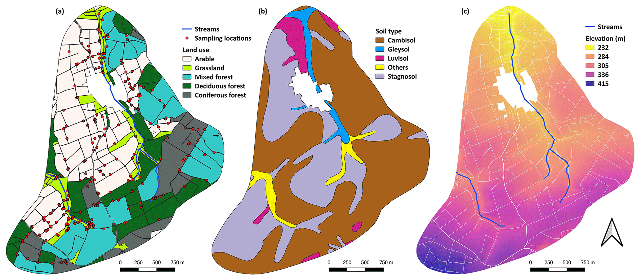
Figure 1 Map showing (a) the land uses and the location of the stratified sampling sites (selected based on combined classes of land use, slope, and soil type) across the study area. (b) The soil types (source: Geoportal Hessen, https://www.geoportal.hessen.de/, last access: 1 March 2022). (c) The digital elevation model (DEM; 1 m resolution) of the landscape (source: Hessische Verwaltung für Bodenmanagement und Geoinformation, https://hvbg.hessen.de/, last access: 1 March 2022).

2.2 Soil physicochemical parameters and GHG fluxes

2.2.1 Point measurements

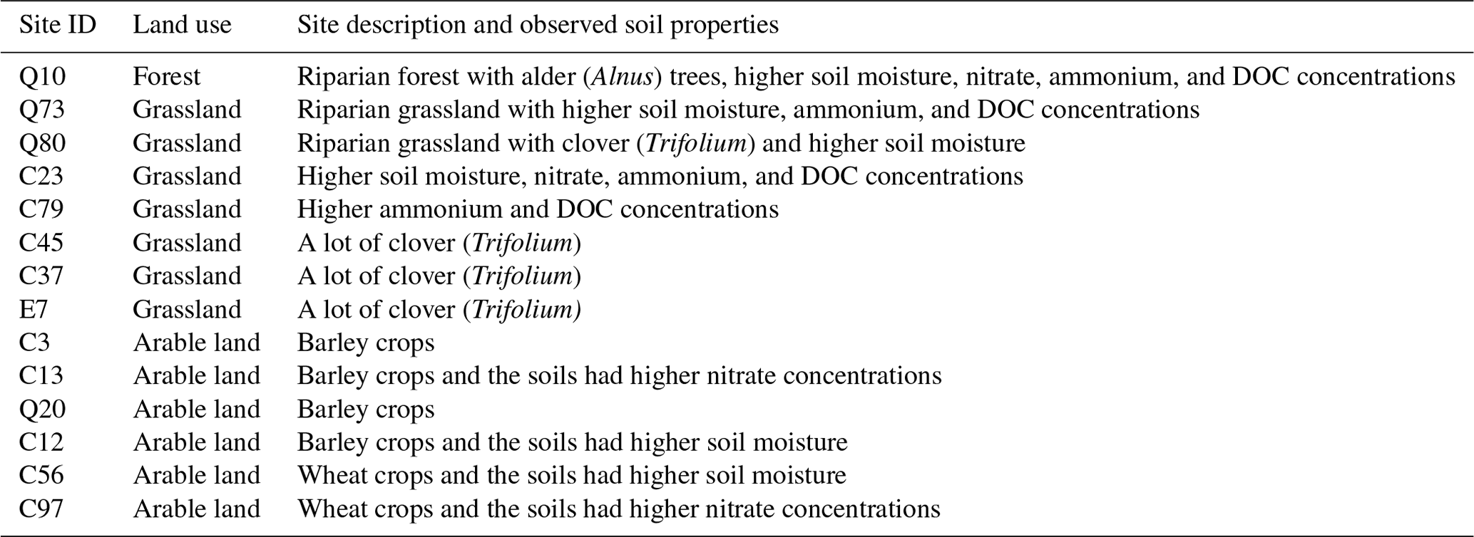
Soil sampling and GHG flux measurements (CH₄, N₂O, and CO₂) were conducted at spatially distributed sampling sites across the study landscape (see Table 1 for a list of observed variables). We used a stratified random sampling approach to distribute 270 sites across different land uses (forest, grassland, and arable), soil types (Cambisol, Stagnosol/Gleysol, and Luvisol), and slopes (0 %–5 %, 6 %–11 %, and >11 %) to capture the spatial variability in the soil GHG fluxes and the driving parameters (Wangari et al., 2022). Out of the 270 targeted locations, field measurements were conducted at 246 sites in the summer (30 June–9 July; field measuring campaign 1) and 268 sites in the autumn (8–17 September; field measuring campaign 2) of 2020. The estimated number of measured points for the forest, grassland, and arable ecosystems was ∼25, 150, and 28 per kilometer squared (Table 1). We allocated more grassland sites due to the hypothesis that riparian grasslands are hot spots of GHG fluxes.

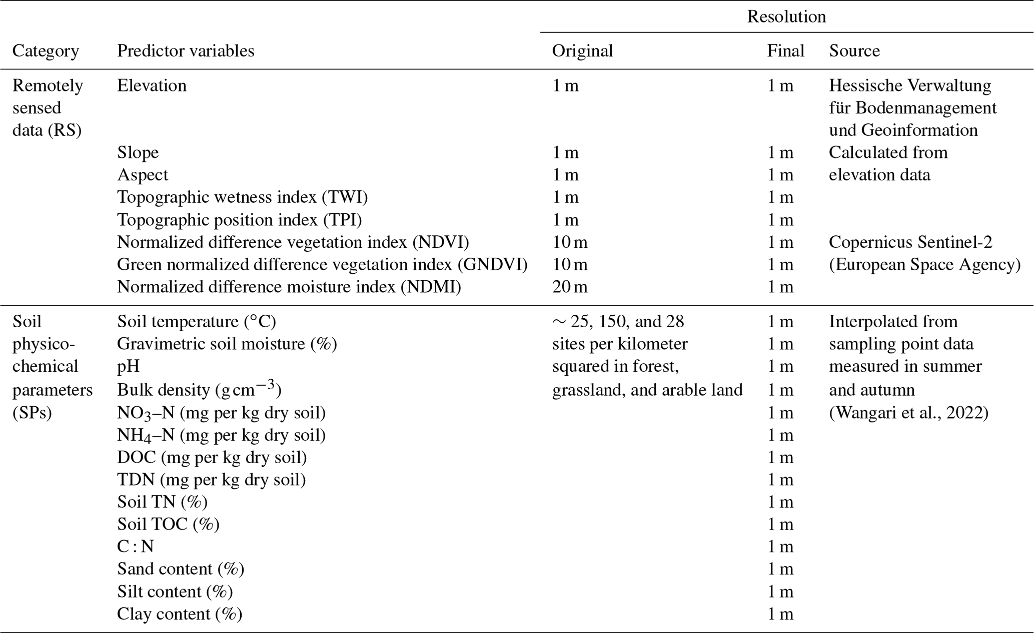
Table 1 List of the soil physicochemical parameters and remotely sensed data used in this study to upscale the GHG fluxes and details of the spatial resolutions of the maps. DOC is dissolved organic carbon, TDN is total dissolved nitrogen, TN is total nitrogen, TOC is total organic carbon, and CN is soil carbon to nitrogen ratio.

Soil GHG flux measurements were performed during the day (07:00–17:00 CEST), using a fast-box chamber technique (Hensen et al., 2013; Butterbach-Bahl et al., 2020). The CO₂ concentrations in the opaque chamber headspace were measured with an infrared gas analyzer (LI-840A and LI-850; LI-COR Biosciences, Lincoln, NE, USA), while CH₄ and N₂O concentrations were measured with an Off-Axis Integrated Cavity Output Spectroscopy (OA-ICOS) analyzer (ABB, Inc., Quebec, Canada). The GHG fluxes were calculated based on the linear changes in the gas concentrations in the chamber headspace in the first 5–7 min following chamber closure. The CO₂ fluxes quantified using the opaque chambers represented either soil respiration (SR) (root and microbial respiration) or ecosystem respiration (ER) (root, microbial, and plant respiration). The CO₂ measurements in autumn across the entire landscape were SR, since the aboveground biomass was not included in the chambers during measurements. In contrast, the summer CO₂ measurements on arable and grasslands were ER, since the aboveground vegetation was incorporated using chamber extensions, while the forest measurements remained as SR due to minimal aboveground vegetation on the forest floor. The day-to-day or diurnal variabilities related to our sampling strategy had a negligible effect on our data, with most of the variability in the data linked to spatial heterogeneities. Details of this finding and the soil sampling, analysis, and flux measurement methods are described in Wangari et al. (2022).

2.2.2 Spatial interpolation of soil parameters

Upscaling soil GHG fluxes using the RF algorithm required spatial raster maps of the soil physicochemical predictor parameters. Thus, we interpolated our measured point data to continuous landscape maps, using the inverse-distance-weighted (IDW) approach in the System for Automated Geoscientific Analyses software (SAGA QGIS), with a distance coefficient power of 1 (Gradka and Kwinta, 2018). The spatial interpolations were performed per land use (forest, grassland, and arable land) and for each season (summer and autumn), due to significant variations in soil parameters such as soil moisture or inorganic N content across land uses and seasons (see Wangari et al., 2022).

2.3 Remote sensing data

We retrieved several landscape-scale remote-sensing images with spatial data representing potential drivers of soil GHG fluxes, such as vegetation cover and vegetation water content. Landscape elevation was acquired from a high-resolution (1 m) digital elevation model (DEM) retrieved from the Hessische Verwaltung für Bodenmanagement und Geoinformation on 1 March 2022 (https://hvbg.hessen.de/). Slope and aspect were calculated from the DEM, using the “r.slope.aspect” function in QGIS (quantum geographic information system). We further computed the topographic position index (TPI) and topographic wetness index (TWI) from the DEM, using the terrain analysis plugin in QGIS. Vegetation information on chlorophyll and water content was derived from satellite bands of Sentinel-2 images. Satellite images with low (<1 %) cloud cover were accessed from the European Space Agency (ESA) Copernicus Open Access Hub (https://scihub.copernicus.eu/; last access: 12 March 2021), using the Semi-Automatic Classification Plugin (Congedo, 2021) in QGIS for each field-measuring period. The normalized difference vegetation index (NDVI) and the green normalized difference vegetation index (GNDVI) were calculated using the near-infrared (NIR), red, and green bands (Bannari et al., 1995; Gitelson and Merzlyak, 1998; Eqs. 1 and 2). Compared to NDVI, GNDVI has a higher ability to detect the differences in the chlorophyll content of plants, especially later in the vegetation period, due to the higher chlorophyll sensitivity of the green band in GNDVI than the red band in NDVI. The vegetation water content was estimated using the normalized difference moisture index (NDMI), which was computed using the near-infrared (NIR) and short-wave infrared (SWIR) bands (Gao, 1996; Malakhov and Tsychuyeva, 2020; Eq. 3). We uniformly downscaled the resolutions of these remotely sensed vegetation indices to match the 1 m spatial resolution of the DEM-derived data files (Table 1).

$$\begin{array}{}\text{(1)}& {\displaystyle }\text{NDVI}={\displaystyle \frac{\text{NIR}-\text{red}}{\text{NIR}+\text{red}}}\text{(2)}& {\displaystyle }\text{GNDVI}={\displaystyle \frac{\text{NIR}-\text{green}}{\text{NIR}+\text{green}}}\text{(3)}& {\displaystyle }\text{NDMI}={\displaystyle \frac{\text{NIR}-\text{SWIR}}{\text{NIR}+\text{SWIR}}}\end{array}$$

2.4 Random forest regression model

RF model development and prediction of the GHG fluxes were performed per land use (forest, grassland, and arable) because there were statistically significant differences observed in the measured fluxes and the underlying GHG flux controls of soil parameters for the different land uses (Wangari et al., 2022). For instance, N₂O fluxes and soil nitrate concentrations were up to 2-fold higher in arable soils than in forestry or grassland soils. The CH₄-uptake rates of grassland and arable soils were lower than those of forest soils, due to general differences in soil structure, nitrogen concentrations, and disturbances (Wangari et al., 2022). Modeling land-use-specific GHG fluxes also enabled the identification of the best remotely sensed predictors, as the dominance of individual GHG production and consumption processes may vary, depending on the specific land use. These best predictors can also be used as benchmark parameters in future studies that use a similar modeling framework to model GHG fluxes in single-land-use landscapes. In contrast to land use, we trained models using merged summer and autumn point data to enable larger and temporally representative datasets for training models that could estimate low- and high-landscape GHG fluxes (Fig. 2).

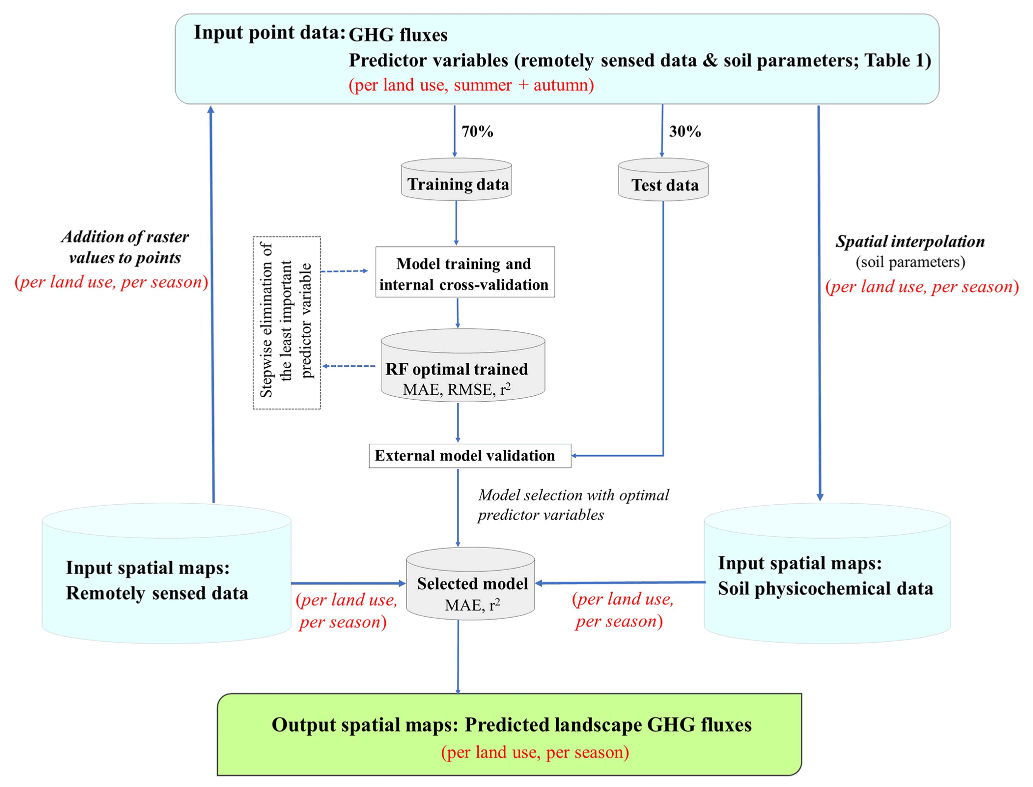
Figure 2 Workflow summary showing the input data (in blue), the approach used for RF model development and prediction of landscape fluxes, and the performance evaluation metrics (MAE, RMSE, and r²).

We used the RF algorithm built in the CARET (classification and regression training) package in R to predict the soil GHG fluxes at a landscape scale (Breiman, 2001; Kuhn, 2008). For model development, the input datasets were split into a training and internal cross-validation set (70 %) and an external test set (30 %), using a stratified random-sampling method. In addition to this hold-out approach of model validation, we defined a 10-fold (K=10) repeated cross-validation scheme on the 70 % dataset, using the “trainControl” function to internally validate our trained models and prevent model overfitting (Berrar, 2019). This model validation strategy also minimized the limitation of the initial hold-out approach, providing a more spatially robust model validation step (Meyer and Pebesma, 2022). A seed value of 123 was specified using the “set.seed” function to enable reproducible results each time we ran a specific model. The random forest's most important hyperparameters (mtry stands for the number of variables at each tree; n.tree stands for the number of trees) were tuned automatically within the CARET package. Tuning was done automatically after a sensitivity analysis (based on assessing the mean absolute error or MAE) was performed 10 times to choose the best mtry and n.tree, resulting in the optimal trained model, i.e., the one with the lowest MAE. The predictor variables in the optimal trained model were then ranked according to their importance, using the RF variable importance measure in the “varImp” function. Subsequently, stepwise elimination of the least essential variable was performed to quantify the predictive power of landscape GHG fluxes using fewer predictor variables (Fig. 2).

To assess the effectiveness of various types of predictors in modeling landscape fluxes, we defined three categories of datasets, namely remote sensing (RS), site-measured soil physicochemical parameters (SPs), and combined data (CD) (Table 1). Several RF models were trained, following the stepwise elimination of the least important variables in each data category (RS, SPs, and CD). Since 88 % of CH₄ fluxes were negative and 86 % of N₂O fluxes were positive (Wangari et al., 2022), we additionally trained models using only the negative CH₄ and positive N₂O flux datasets to compare their performances with the models built with all (positive and negative) fluxes.

2.5 Model performance assessment and prediction of landscape fluxes

The performance assessment metrics of the trained models included MAE, root mean square error (RMSE), and the coefficient of determination (r²) from the internal cross-validation. The final models for predicting landscape fluxes in each data category (RS, SPs, and CD) were selected based on the highest possible r² with a relatively low MAE. For each season and land use, the surface maps of the respective predictor variables in the final models were merged using the raster brick function in R. The spatial fluxes for each land use were then predicted based on the selected model and the input raster brick, using the “predict” function in R. To improve the prediction performance, the non-normal distributed (SR/ER_CO₂ and N₂O) fluxes were log-transformed before model development. After prediction, the transformed fluxes were retransformed using an exponential function.

Further evaluation of the model performances was conducted through linear regression and correlation analysis of observed against retransformed predicted fluxes for all sampling sites. An additional external validation step was performed using the measured and predicted fluxes of the sampling sites in the 30 % test dataset that was excluded from the model development. For this analysis, we compared the predicted mean fluxes (using RS, SPs, and CD datasets) with the observed mean fluxes. Analyses of variances (type II) from linear mixed-effects models (“nlme” package in R) were used to compare these arithmetic means. The fixed effects in the mixed models were seasons (summer and autumn) and GHG flux type (measured and predicted fluxes from the RS, SPs, and CD datasets). Random effects of site variability were also included in the mixed models. The measured and predicted fluxes were log-transformed to the normality assumption. A Tukey post hoc test (p value<0.05) of the least square means was used on the mixed models to identify statistically significant differences between the measured, RS-predicted, SP-predicted, and CD-predicted fluxes.

Since many traditional GHG upscaling approaches rely on aggregated fluxes (area-weighted averages), we also estimated spatial fluxes for the summer and autumn seasons using this technique. GHG fluxes were aggregated on the landscape scale by multiplying the average fluxes measured for each land use by the area of each land use. We compared the total landscape fluxes upscaled using this conventional aggregation technique of average fluxes with the spatial fluxes predicted using the modeling approach.

2.6 Identification of summer and autumn GHG “hot” and “cold” spots from predicted landscape fluxes

Statistical approaches were deployed to identify areas that may have disproportionately contributed to the overall landscape GHG fluxes (e.g., van Kessel et al., 1993; Mason et al., 2017). We defined the threshold for hot spots using the sum of the median (M) flux and the interquartile (Q3−Q1) flux range (Eq. 4). Thus, the hot spots within the landscape were identified as being the areas with flux values greater (lower for CH₄ uptake) than the set hot spot threshold. We fixed an inverse threshold (Eq. 5) for cold spots and identified cold-spot patches with fluxes below (above for CH₄ uptake) this threshold. Common emission hot spots were defined as the areas with overlapping elevated emissions of the three GHG fluxes (SR/ER–CO₂, CH₄, and N₂O) within the landscape. The average (summer and autumn) landscape fluxes were used to identify the hot and cold spots. We also calculated season-specific thresholds to compare the increase and decrease in the hot- and cold-spot areas between summer and autumn.

$$\begin{array}{}\text{(4)}& {\displaystyle }\text{Hot spot threshold}=M+(Q\mathrm{3}-Q\mathrm{1})\text{(5)}& {\displaystyle }\text{Cold spot threshold}=M-(Q\mathrm{3}-Q\mathrm{1})\end{array}$$

3 Results

3.1 RF model performance

The performance of the final models selected for the prediction of landscape fluxes varied across input datasets (RS, SPs, and CD), GHG fluxes (SR/ER_CO₂, CH₄, and N₂O), and land use (forest, grassland, and arable land) (Table 2). The predictive performance (r²) from the internal cross-validation step was higher in the models using the CD dataset (0.15–0.78 range) than those using the RS (0.13–0.73 range) and SP (0.15–0.63 range) datasets (Table 2). The RF models predicting SR/ER_CO₂ fluxes had much higher r² (0.45–0.78 range) than those predicting N₂O and CH₄ fluxes (0.13–0.56 range). Arable ecosystem models resulted in much better predictions of SR/ER_CO₂ (r²; 0.63–0.78 range) and N₂O (r²; 0.45–0.56 range) fluxes compared to those for forest and grassland ecosystems across all data categories (Table 2). The prediction of CH₄ fluxes was also better for arable lands but only when using the RS data (Table 2). Stepwise elimination of the least important variables had a minimal effect on the performances of the trained models (Tables B1–B5). The selected models for the different categories of datasets (RS, SPs, and CD) had varying predictor variables across land uses. The forest and grassland models required the most (five and six) predictor variables. In contrast, the least number of predictors (two) were mainly observed for models describing GHG fluxes from arable soils, especially in the RS and SP categories (Table 2).

Table 2 List of predictor variables and the performance of the selected RF models, using either remote sensing (RS), soil physicochemical parameters (SPs), or combined (remote sensing and soil parameters) data. The model selection was made after a cross-validation (10-fold) step, whereby the model's predictive power was tested based on unseen data to avoid overfitting. SN is the measured soil nitrogen content.

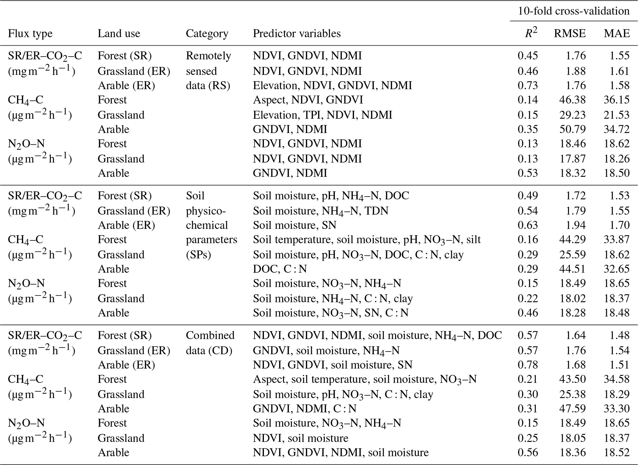
Comparing the models (CD) applied to predict the landscape fluxes, the site-measured soil moisture content was a key predictor variable for all three GHG fluxes across land uses. In addition to soil moisture, the measured soil nitrogen content (NH₄ or SN) and remotely sensed vegetation indices (NDVI, GNDVI, or NDMI) were prevalent predictors of landscape SR/ER_CO₂ fluxes. Soil nitrogen content (NO₃ or CN) was also a recurrent predictor of CH₄ fluxes across land uses. However, the landscape CH₄ models had other varying predictors, such as aspect and soil temperature in forest models, pH and clay in grassland, and vegetation indices in arable ecosystem models. For N₂O, soil inorganic nitrogen (NH₄ or NO₃) concentrations predicted the fluxes in the forested areas, while vegetation indices were common predictors in grassland and arable ecosystems (Table 2).

Further assessment of model performance was performed through an external validation step comparing the mean of observed and predicted fluxes in the test dataset ($n=\sim \mathrm{140}$ per flux). The mean measured CO₂ and CH₄ fluxes were similar to the predicted carbon fluxes across all the data categories (RS, SPs, and CD) within each season. In contrast to the carbon fluxes, the measured N₂O fluxes were significantly lower than the predicted fluxes in autumn (Fig. A1).

3.2 Observed versus predicted GHG fluxes

The measured and predicted GHG fluxes for all the sampling points had significant (p<0.001) linear relationships (Fig. 3). The model predictions of SR/ER_CO₂ fluxes were better (r²; 0.49–0.67) than for soil CH₄ (r²; 0.39–0.46) or N₂O (r²; 0.34–0.43) flux predictions across the three input datasets. Based on the estimated slopes, the predicted values were 35 %–46 % lower than the measured values for SR/ER_CO₂ fluxes. Compared to CO₂, the CH₄ and N₂O predicted fluxes were lower (CH₄ 53 %–58 %; N₂O 60 %–65 %) than the measured fluxes, primarily due to the underestimation of high fluxes. Based on r² values, the performances of the different predictor datasets were on the order of $\text{CD}>\text{RS}>\text{SP}$ for carbon fluxes and $\text{CD}>\text{SP}>\text{RS}$ for N₂O fluxes (Fig. 3).

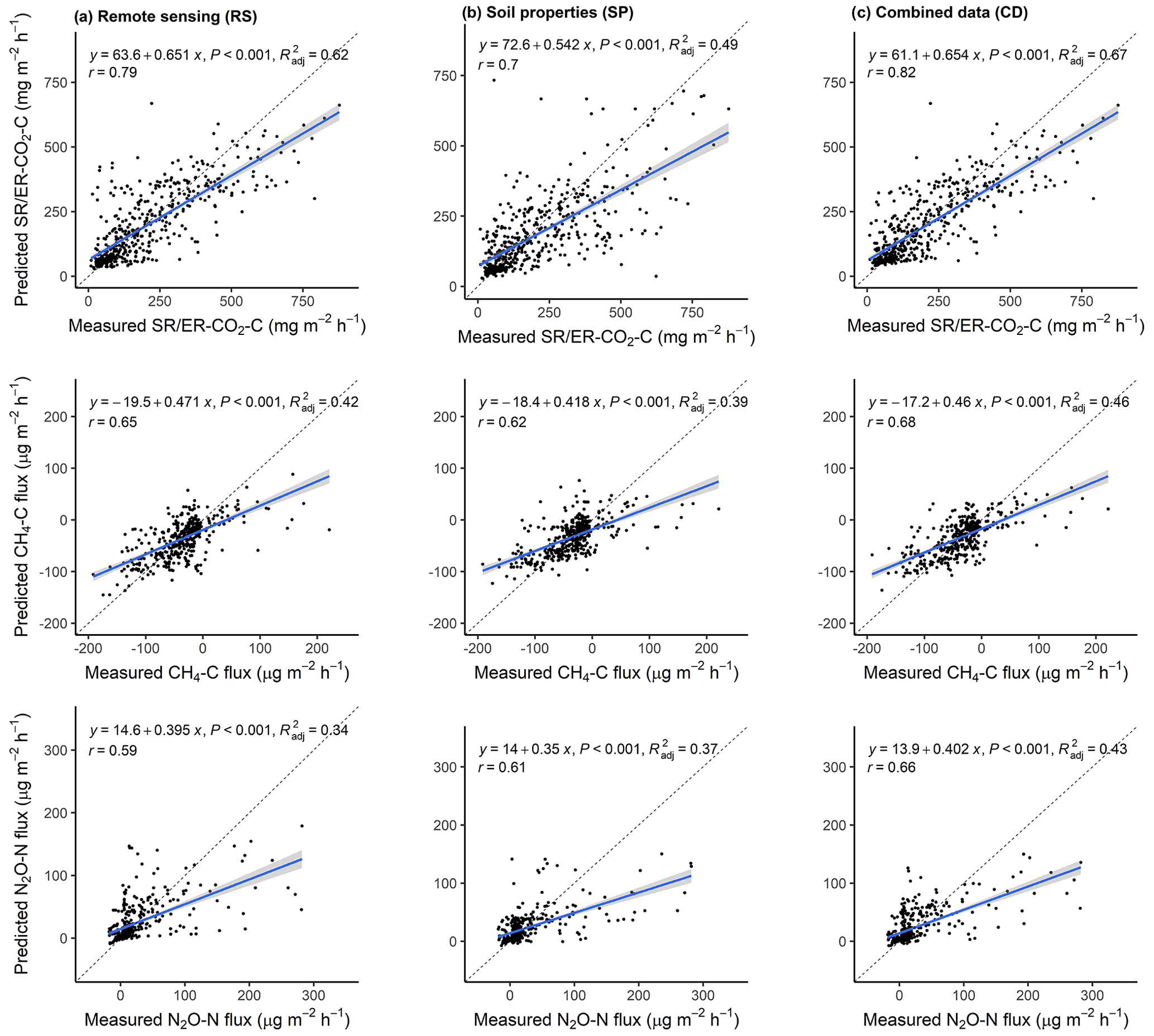
Figure 3 Linear regressions (with 95 % confidence bands) of the measured and predicted GHG fluxes, using remotely sensed data (RS), soil physicochemical parameters (SPs), and combined data (CD). GHG fluxes from all the sampling locations (both the 70 % training data and the 30 % test data) were considered in this regression analysis. The dotted line represents the 1:1 line.

3.3 Spatiotemporal variation in modeled landscape-scale fluxes

Predicted landscape fluxes for the summer and autumn seasons ranged from +27.7–+733.3 $\mathrm{mg}{\mathrm{m}}^{-\mathrm{2}}{\mathrm{h}}^{-\mathrm{1}}$ for CO₂–C and −148.4–+89.4 $\mathrm{\mu }\mathrm{g}{\mathrm{m}}^{-\mathrm{2}}{\mathrm{h}}^{-\mathrm{1}}$ for CH₄–C to −8.8–+189.9 $\mathrm{\mu }\mathrm{g}{\mathrm{m}}^{-\mathrm{2}}{\mathrm{h}}^{-\mathrm{1}}$ for N₂O and did not differ much in dependence of the input dataset used (RS, SPs, or CD) (Table B6). However, the predicted flux ranges for the landscape were narrower than the measured fluxes, which ranged from 8.7 to 877.0 $\mathrm{mg}{\mathrm{m}}^{-\mathrm{2}}{\mathrm{h}}^{-\mathrm{1}}$ for CO₂–C and −214.1–+221.2 $\mathrm{\mu }\mathrm{g}{\mathrm{m}}^{-\mathrm{2}}{\mathrm{h}}^{-\mathrm{1}}$ for CH₄–C to −18.1–+281.8 $\mathrm{\mu }\mathrm{g}{\mathrm{m}}^{-\mathrm{2}}{\mathrm{h}}^{-\mathrm{1}}$ for N₂O–N. Since the CD dataset revealed models with better predictions for all GHG fluxes than the RS and SP datasets, we used GHG fluxes predicted from CD predictors for seasonal and land use comparisons.

Most of the landscape area (99.2 %) had higher SR/ER_CO₂ fluxes in summer than in autumn, with a small proportion of arable and grassland ecosystems having an opposite trend. Around 76 % of the landscape also had higher N₂O fluxes in summer than in autumn. Approximately 24 % of the landscape, primarily in the forested areas, had higher N₂O fluxes in autumn than in summer. CH₄-uptake rates were lower in summer than in autumn in most of the landscape (63 %), especially in arable and grassland soils. However, an opposite trend was found for about 37 % of the landscape area, dominated by forests, where CH₄-uptake rates were lower in autumn than in summer (Fig. 4c).

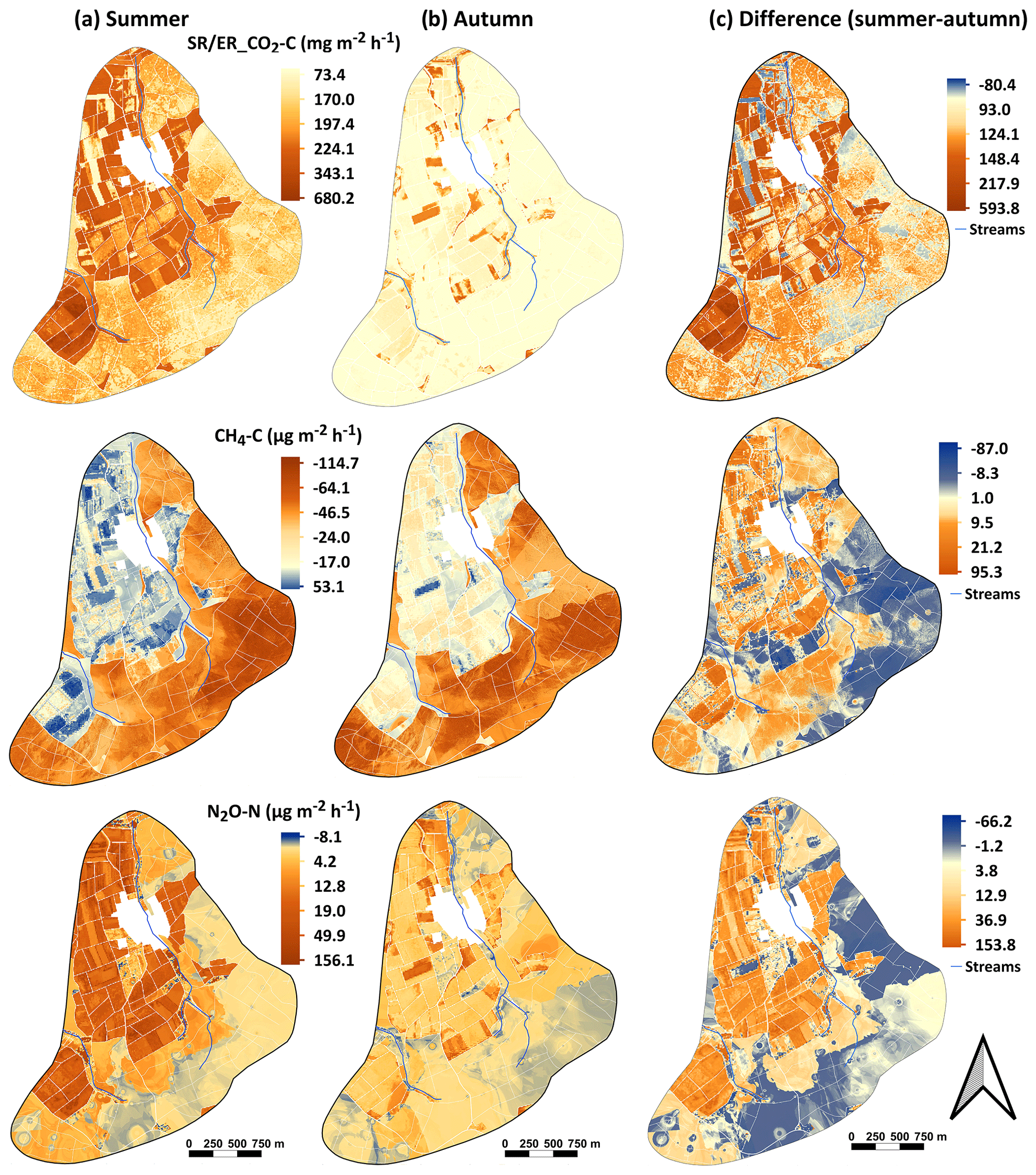
Figure 4 Landscape maps of SR/ER_CO₂, CH₄, and N₂O for (a) summer, (b) autumn seasons, and (c) the difference maps showing the variation in the autumn from the summer fluxes. The surface fluxes were predicted using RF models trained with combined (remote-sensing and site-measured soil parameters) data (CD; Table 2).

High spatial heterogeneities (within short distances of <2 m) of the predicted landscape fluxes were observed in each land use. Overall, spatial variations were more prominent in summer than in autumn (Fig. 4 and Table B6). The spatial variability in the SR/ER_CO₂ fluxes was higher (with a range of up to 2.6-fold) on arable soils than forest and grassland soils, with multiple patches of low fluxes surrounded by high fluxes. CH₄ fluxes on arable lands were also heterogeneous, with the soil acting as CH₄ sinks and sources within a few meters, especially during summer (Fig. 4a). For N₂O fluxes, high spatial heterogeneities were observed on grassland soil in summer, as N₂O uptake and emission of the same or even higher order of magnitude occurred at neighboring pixels. Arable soils were also highly heterogeneous, with patches of high N₂O fluxes surrounded by low fluxes in autumn (Fig. 4b).

3.4 Summer and autumn hot spots and cold spots

The hot and cold spots of the GHG fluxes were identified from the average (summer and autumn) upscaled landscape fluxes (Fig. 5a). Using Eq. (4), the SR/ER_CO₂ and N₂O spatial hot spots had threshold values >231.5 $\mathrm{mg}{\mathrm{CO}}_{\mathrm{2}}\text{-}\mathrm{C}{\mathrm{m}}^{-\mathrm{2}}{\mathrm{h}}^{-\mathrm{1}}$ for CO₂ and >36.8 $\mathrm{\mu }\mathrm{g}{\mathrm{N}}_{\mathrm{2}}\mathrm{O}\text{-}\mathrm{N}{\mathrm{m}}^{-\mathrm{2}}{\mathrm{h}}^{-\mathrm{1}}$ for N₂O. These hot spots covered a relatively small portion (∼16.7 %) of the landscape, yet they played a significant role, especially the N₂O hot spots, which accounted for 42 % of the landscape fluxes. Around 29 % of the total SR/ER_CO₂ landscape flux emanated from the hot spot areas (Fig. 5). Overall, the SR/ER_CO₂ and N₂O hot spots were mainly located on arable lands (77.0 % and 94.5 %, respectively) and grasslands (22.9 % and 5.5 %, respectively). Compared to the SR/ER_CO₂ and N₂O hot spots, the hot and cold spots of CH₄ uptake were observed in smaller regions (3.1 % and 7.3 %) of the landscape, with high soil CH₄-uptake rates (>87.3 $\mathrm{\mu }\mathrm{g}{\mathrm{CH}}_{\mathrm{4}}\text{-}\mathrm{C}{\mathrm{m}}^{-\mathrm{2}}{\mathrm{h}}^{-\mathrm{1}}$) and low soil CH₄-uptake rates (<3.4 $\mathrm{\mu }\mathrm{g}{\mathrm{CH}}_{\mathrm{4}}\text{-}\mathrm{C}{\mathrm{m}}^{-\mathrm{2}}{\mathrm{h}}^{-\mathrm{1}}$). The CH₄-uptake hot spots, exclusively on the forested soils, offset 8 % of the landscape CH₄ fluxes (Fig. 5). The cold spots occupied 7 % of the landscape and were primarily on arable soils (99.6 %), accounting for 2 % of the landscape's CH₄ emissions.

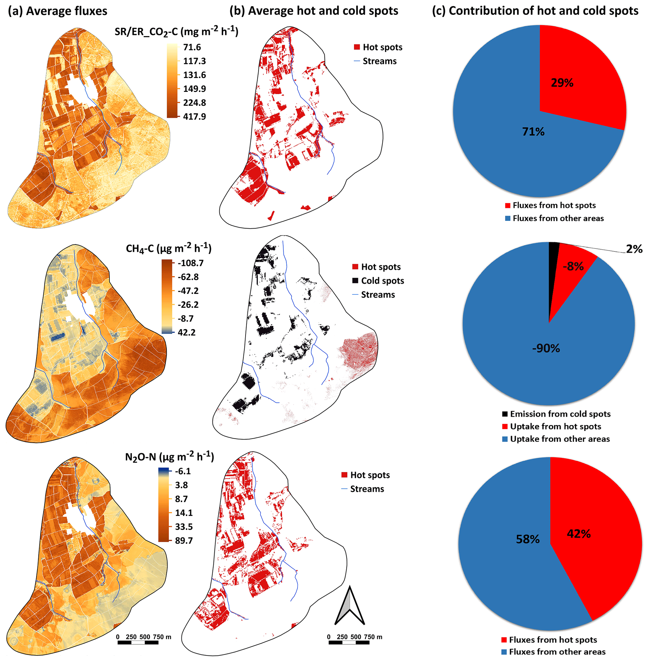
Figure 5 Maps showing (a) the average GHG fluxes and (b) the average hot-spot and cold-spot regions on the landscape for the summer and autumn seasons. The pie charts show the contribution (%) of hot and cold spots to total landscape fluxes. For this analysis, landscape fluxes were predicted using the combined data (CD; Table 2 and Fig. 3).

Common hot spots, with overlapping areas with elevated GHG emissions (i.e., SR/ER_CO₂ and N₂O hot-spot areas and CH₄-uptake cold-spot areas) were mainly on arable soils (99.87 %), with a few located in grasslands (0.12 %) and forests (0.01 %). Overall, these patches covered 1.5 % of the landscape area and contributed 5 %, 1 %, and 8 % of the SR/ER_CO₂, CH₄, and N₂O emissions within the landscape (Fig. A2). Based on field observations of the sampling sites (n=14) in the common hot spots, the sites at arable lands were either cropped with barley or wheat. These arable common hot spots also had higher soil moisture content and NO₃ concentrations than the average values recorded at all the other sampling locations. The common hot spots in the forest were found along the riparian zones if either nitrogen-fixing alder trees were present or if grazed by cattle. Soil moisture (%), dissolved organic carbon (DOC), NO₃, and NH₄ concentrations at these sites were also higher than mean values across all sampling points. The grassland common hot-spot regions were densely covered by nitrogen-fixing clover, with some located along the riparian zones (Fig. A3 and Table B7).

Comparison of the GHG emission hot spots in summer and autumn using season-specific thresholds revealed significant shifts in their geolocations between the two seasons (Fig. A4). SR/ER_CO₂ hot-spot regions expanded by 46 % from summer to autumn, even though the emissions from the former season were higher. Unlike CO₂, N₂O emission hot spots and CH₄-uptake cold spots contracted by 23 % and 86 %, respectively, from summer to autumn.

3.5 Comparison of upscaling approaches

Seasonal differences in spatial patterns and magnitudes of GHG fluxes were observed for upscaled fluxes, using either RF modeling or mean values of measured fluxes. In both approaches, the SR/ER_CO₂ and N₂O landscape fluxes were an order of magnitude higher in summer than in autumn. The CH₄-uptake rates were higher in autumn than in summer but within the same order of magnitude. In summer, the landscape-scale SR/ER_CO₂ and N₂O fluxes estimated using the area-weighted average approach were 26 % and 50 % higher than the RF-modeled fluxes. The contrary was observed in autumn, where the later methodology produced slightly higher fluxes (4 % and 11 %) than the area-weighted mean estimates.

The entire landscape CH₄-uptake estimates for autumn using the area-weighted mean were 16 % higher than the modeled estimates. Contrary to autumn, the area-weighted mean approach had slightly lower estimates of CH₄ uptake than the modeling approach in summer. Additionally, the CH₄ surface flux estimates for the whole arable land in summer were net sinks (−0.9 CH₄-C g h⁻¹) using the RF modeling approach, contrary to the net sources (15.5 CH₄-C g h⁻¹) estimated by the area-weighted mean method. Overall, the total landscape fluxes estimated using the area-weighted mean approach had up to 2 orders of magnitude higher uncertainty (standard error) than the modeled landscape fluxes (Fig. 6).

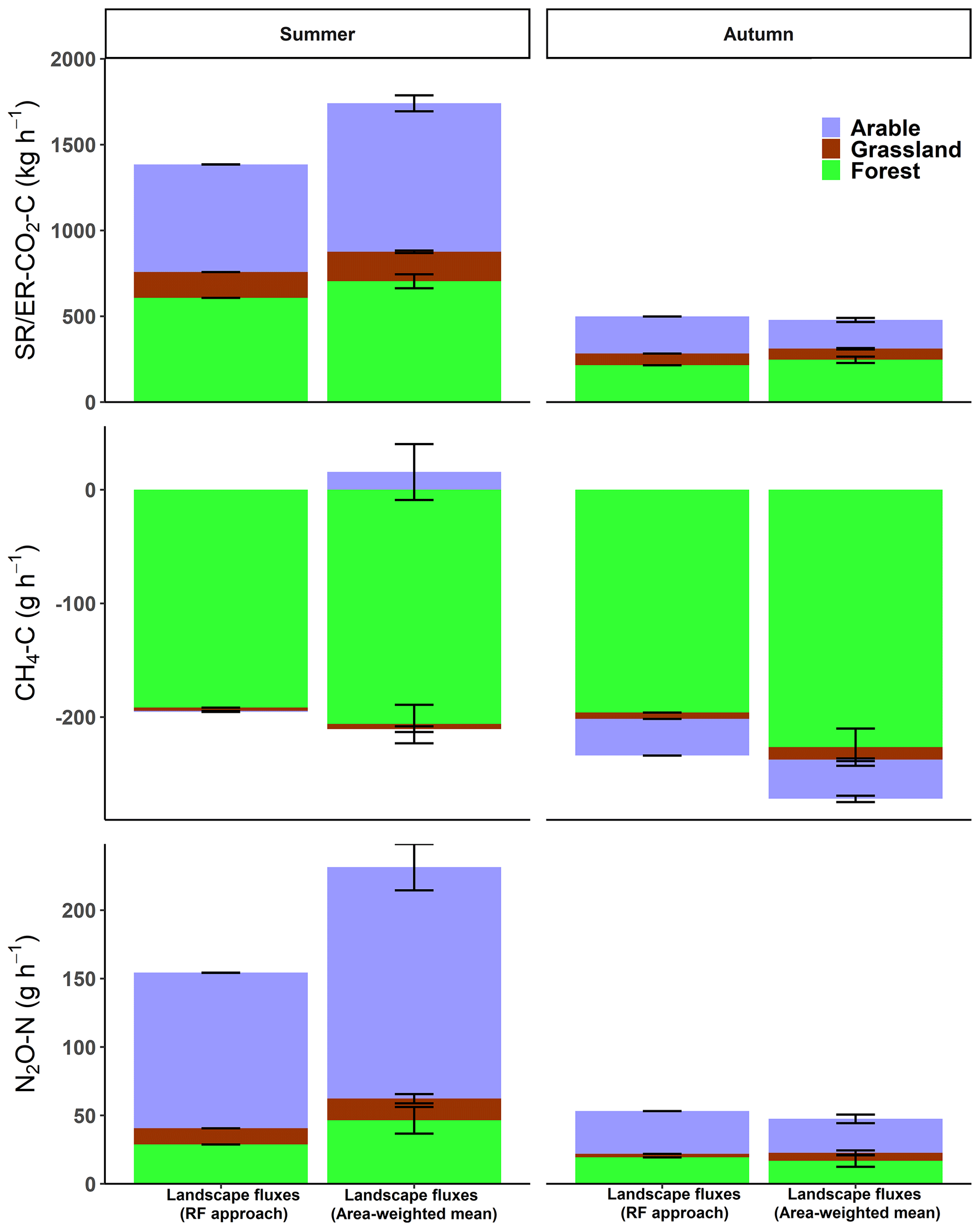
Figure 6 The total landscape fluxes (±SE) predicted using random forest (RF) models (with combined dataset) and the fluxes estimated using the area-weighted mean approach, where the average point-measured fluxes were multiplied by the landscape area.

4 Discussion

4.1 Efficiency of in situ soil parameters and remote-sensing data in upscaling GHG fluxes

Our study showed that remotely sensed (RS) data and measured soil parameters (SPs) could effectively upscale soil–atmosphere CO₂, N₂O, and CH₄ fluxes from point chamber measurements across a heterogeneous landscape with mixed land uses. This approach represents a tier-3 approach of upscaling landscape GHG fluxes, as it provides spatially explicit GHG fluxes at a high resolution that is comparable to modeled fluxes using either process-based models or statistical functions (e.g., Haas et al., 2013; Tiemeyer et al., 2020; Koch et al., 2023). The improved prediction performance of the combined data (CD) sources indicates the importance of incorporating controls of soil GHG fluxes that are remotely sensed and ground-based field observations. The prediction models in this study suggested that the Sentinel-2-derived indices (NDVI, GNDVI, and NDMI) were more effective predictors than the DEM-derived terrain attributes (elevation, slope, aspect, TWI, and TPI). This finding is supported by the appearance of the Sentinel-2-derived indices in the prediction models of the three GHGs, contrary to only one DEM index (aspect) that appeared in the CH₄ flux prediction models for the forest ecosystem. The minor role of DEM indices in this study can be attributed to the relatively flat terrain of our study landscape (Fig. 1b) and is further backed by the lack of spatial variation in the measured GHG fluxes with slope, yet slope was considered during site stratification (Wangari et al., 2022). Another possible explanation could be that soil wetness, a common predictor of all the GHG fluxes across the landscape, was better represented by the site-measured soil moisture content and the NDMI index (vegetation water content) than any of the DEM terrain attributes, including the TWI that focuses on moisture conditions, as they lack a temporal dimension.

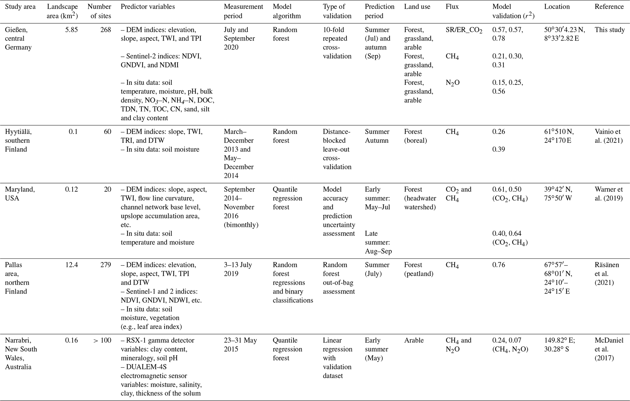
Compared with other studies that have upscaled GHG fluxes using the random forest algorithm, we considered more site-measured data on soil parameters, all three GHG fluxes, and different land uses (Table 3). Moreover, point selections for measurements were made by implementing a stratified sampling plan that represented the spatial variability in the several landscape characteristics, specifically land use, soil type, and slope (Wangari et al., 2022). The prediction accuracies of soil respiration for our mixed-forest ecosystem (3.3 km²) were slightly better than those reported for a smaller forested headwater watershed (0.12 km²) in Maryland, USA (Warner et al., 2019). Our CH₄ prediction performance for forest soils was comparable to those of a boreal forest landscape (Vainio et al., 2021). However, our CH₄ prediction performance was up to 3.6-fold lower than those of a forested headwater watershed and peatland soils, which can be attributed to higher and more homogenous CH₄ production in such ecosystems (Warner et al., 2019; Räsänen et al., 2021). Our CH₄ and N₂O model prediction accuracies for arable soils were better than those for arable soils in New South Wales, Australia, which only considered input data from ground-based sensors such as soil pH and clay content (McDaniel et al., 2017). Nevertheless, caution has to be taken when interpreting any conclusions from these study comparisons due to the limitations of different model validation techniques, different predictor variables used for modeling, and the different ecosystems and spatial scales of measurement and predictions.

Table 3 Comparison with other studies that have upscaled landscape fluxes using the random forest algorithm. TRI is for terrain ruggedness index, DTW is for cartographic depth-to-water index, and NDWI is for normalized difference water index.

4.2 Seasonal variability in the landscape fluxes

The GHG fluxes predicted by the RF model in this study revealed seasonal trends of up to 3-fold higher CO₂ and N₂O fluxes in summer and 1.2-fold higher CH₄ uptake in autumn, which were also evident in the measured fluxes at the sampling points (Wangari et al., 2022). These trends can be attributed to seasonal changes in soil parameters and vegetation within the landscape that were well captured by the measured soil parameters and Sentinel-2-derived indices in the prediction models. The higher soil moisture, mineral nitrogen, and vegetation cover observed during the summer growing season enhanced the respiration rates (SR/ER_CO₂) and N₂O emissions, particularly in arable ecosystems, which were flux hot spots for both gases. Root respiration of growing plants can also enhance N₂O production through denitrification by creating anaerobic conditions and supplying labile exudates to denitrifying microbes (Butterbach-Bahl and Dannenmann, 2011; Malique et al., 2019). Previous studies have shown that higher mineral nitrogen and soil moisture content can enhance N₂O production in soils through an increased supply of substrates and the creation of anaerobic conditions that enhance denitrification rates (Barton et al., 1999; Ciarlo et al., 2007; Butterbach-Bahl et al., 2013). The lower CH₄-uptake rates in summer can be primarily explained by the observed higher soil moisture content, which has been previously reported to hinder CH₄ oxidation by slowing down gas (atmospheric CH₄) diffusion in soils (Le Mer and Roger, 2001).

The high-resolution (1 m pixel size) scaled-up fluxes could also identify the detailed temporal patterns of the GHG fluxes across the landscape, thus revealing trends that were otherwise undetectable in the aggregated measured (point) fluxes. To illustrate, parts of the landscape (24 % and 37 %) showed even opposite trends of higher N₂O fluxes and lower CH₄-uptake rates in autumn, and these areas were predominantly in the mixed-forest ecosystem. Such fine-scale patterns of GHG fluxes result from land-use-specific local effects, depending on the season. For example, decaying fallen leaves during autumn can favor denitrification in forest soils by increasing carbon and mineral N availability (e.g., Groffman and Tiedje, 1989), which may not be true for grassland or arable ecosystems due to harvesting and mowing. The higher CH₄-uptake rates in summer could be due to warmer summer temperatures leading to drier, more aerated forest soils that promote CH₄ oxidation (Steinkamp et al., 2000). This finding is supported by the importance of aspect as a predictor of landscape CH₄ fluxes in the forest ecosystem, which influences the amount of incoming radiation an area receives.

4.3 Importance of hot spots and cold spots of landscape-scale GHG fluxes

The high spatial resolution of our predicted GHG fluxes enabled the identification of areas across the landscape that functioned as hot spots (of soil CH₄ uptake, SR/ER_CO₂, and N₂O) or cold spots of soil CH₄ uptake. Based on field observations and analyses of important predictor variables, the existence of these hot and cold spots was primarily driven by human activities such as fertilizer application, crop growing and tillage, and landscape environmental parameters related to seasonality and proximity to riparian areas. This finding is supported by the primary association of the SR/ER_CO₂ and N₂O hot spots and CH₄-uptake cold spots within arable ecosystems, since these systems showed higher soil mineral nitrogen concentrations than grassland and forest soils. The hot spots of SR/ER_CO₂ and N₂O observed on the grassland ecosystem can be attributed to the primary location of grasslands along the riparian areas. Increased soil moisture values and higher soil C contents, key characteristics of the riparian regions, have also been reported to drive elevated soil GHG fluxes (Kaiser et al., 2018; Vainio et al., 2021).

Spatial hot spots of SR/ER_CO₂ and N₂O played a crucial role in determining total landscape fluxes, accounting for up to 42 % of the total predicted landscape fluxes, despite their relatively low (∼16 %) coverage area. Such high contributions suggest that failure to capture these hot spots results in large uncertainties in the landscape GHG flux estimates. Overall, the contribution of the hot spot areas (of CO₂, N₂O, and CH₄ emissions) to the landscape fluxes decreased on the order of ${\mathrm{N}}_{\mathrm{2}}\mathrm{O}>{\mathrm{CO}}_{\mathrm{2}}>{\mathrm{CH}}_{\mathrm{4}}$. This finding emphasizes the importance of increasing the spatial coverage of N₂O measurements to include more hot spot areas, as they can introduce enormous uncertainty in landscape fluxes if not quantified. A similar finding emphasizing the importance of N₂O flux heterogeneities has been concluded in a previous study, which recorded more sampling locations required for improved N₂O flux estimates than CO₂ and CH₄ at a landscape scale (Wangari et al., 2022).

Identifying common patches with elevated emissions of all three GHGs can inform priority areas for implementing localized mitigation measures within a landscape. These common patches covered only 1.5 % of our landscape (∼0.2 km²) and had the highest GHG fluxes contributing around 5 %, 1 %, and 8 % of the landscape CO₂, CH₄, and N₂O emissions. The location of these patches primarily (99.9 %) on arable land emphasized the significant role of focusing on mitigating GHG fluxes from arable soils. Because most of the common GHG hot spots in the arable soils were also in areas with high water content, mitigation strategies that aim to adjust the fertilizer application rates at specific areas holding more water may successfully lower the emissions (e.g., Hassan et al., 2022). In contrast to hot spot regions of elevated GHG emissions, CH₄-uptake hot spots inform future mechanisms for leveraging the GHG sink ability of soils, such as expanding local forests. This finding is supported by uptake hot spots identified on forest soils in this study, offsetting 8 % of the total landscape CH₄ flux. The expansion of forested areas will also likely have a high mitigation impact via CO₂ sequestration. Although some of the above strategies are currently applied at broader scales (1 km²), localized mitigation strategies may be required at smaller scales (<100 m²), especially at highly heterogeneous landscapes with a high variability in the agricultural practices. We also found significant shifts in the geolocations of hotspot regions between summer and autumn, suggesting that seasonal effects of land management (e.g., fertilization, harvesting, and residue management) and soil conditions may also lead to a temporal expansion or contraction of the hot spot regions. This finding further emphasizes the need for time-based mitigation strategies, such as considering fertilizer application times, which not only target the spatial hot spots but also consider the temporal patterns that result in peak emissions (e.g., Wagner-Riddle et al., 2020).

4.4 Comparison of upscaling approaches

Contrary to the area-weighted upscaling approach of spatial aggregation of chamber fluxes (Webster et al., 2008; Molodovskaya et al., 2011; Rosenstock et al., 2016), random forest modeling allowed us to estimate the entire spatial distributions of the fluxes at high spatial resolution (1 m pixel size), capturing both cold spots and hot spots. In agreement with our hypotheses, the landscape fluxes were either over- or underestimated by the area-weighted average approach compared to the RF modeling approach. The overestimated landscape CO₂ and N₂O fluxes by the area-weighted average approach of up to 50 % during the peak summer season suggest an overrepresentation of the high fluxes measured at most of the sampling points, resulting in elevated mean and upscaled fluxes. Furthermore, landscape CH₄-uptake rates were overestimated by the area-weighted average approach during the peak autumn season. Previous studies have also observed a similar trend of elevated mean CH₄-uptake rates at measured sites, which they attributed to the overrepresentation of high-uptake rates during the peak-uptake seasons (Warner et al., 2019). Conversely, the underestimation of CO₂, N₂O, and CH₄ uptake by the area-weighted average approach, especially on arable soils, coincided with the low-flux season, implying reduced mean fluxes due to the overrepresentation of the low fluxes. An alternative explanation of the differences in landscape flux estimates from both approaches could be the underestimation of high fluxes by the RF models, which we also found in our study. However, the landscape means of RF predicted and measured fluxes from 30 % of our sampled sites were primarily similar (Fig. A1), suggesting that the lack of spatial representation of all hot and cold spots by the area-weighted mean approach rather than the inability of the RF models to reproduce high values accounted for the findings above.

Collectively, our results illustrated that the representativeness of landscape fluxes using aggregated chamber fluxes might be influenced by the spatial and temporal heterogeneity of the fluxes. This finding aligns with previous results on the required number of chamber measurement locations for reliable landscape fluxes that varied with land use and season (Warner et al., 2019; Wangari et al., 2022). The high (50 %) overestimation of landscape N₂O fluxes suggested the higher sensitivity of reliably estimating N₂O fluxes using the (aggregated means) conventional method. Previous studies have also emphasized the importance of N₂O fluxes in constraining uncertainties in landscape flux quantification (e.g., Wangari et al., 2022). Compared to the suggested way of lowering landscape-scale flux uncertainties in the conventional estimates by increasing the number of chamber measurements within a landscape (Wangari et al., 2022), the modeling approach can be a less resource-intensive alternative.

Combining high-resolution remote sensing data and measured soil parameters to upscale the chamber fluxes reduced the biases and the aforementioned landscape-scale flux uncertainties. The reduced uncertainties in the modeled landscape fluxes can be attributed to the relation of multiple underlying controls of soil GHG fluxes, which have high seasonal and spatial variability. Remote sensing datasets have unlimited spatial extents with high spatial resolution, thus allowing reliable prediction of spatially continuous fluxes that can capture the cold and hot spots over different seasons across heterogeneous landscapes (Warner et al., 2019; Räsänen et al., 2021). This study's high spatial resolution upscaling (1 m pixel size) enabled capturing small-scale variabilities in GHG fluxes within short distances, which would have been missed with coarser-resolution upscaling. Upscaling at a finer resolution was especially relevant, due to the heterogeneous nature of our study landscape, which is related to different land uses, soil types, and slope positions.

Notably, the applicability of this upscaling approach largely depends on the availability of spatially extensive chamber measurements. In this study, the 70 % modeling dataset represented data from ∼20 stratified chamber locations per kilometer squared on the arable land and ∼16 chambers per kilometer squared in the forest. These number of chamber measurement locations are within the range of those recommended (29 for arable and 13 for forest) by Wangari et al. (2022) for accurate quantification of landscape GHG fluxes. Based on these findings, these chamber numbers may apply to other studies looking to upscale GHG fluxes using a combination of chamber measurements and remotely sensed data. However, the feasibility of this adoption will highly depend on the level of similarities in landscape properties with our study.

5 Conclusions

This study demonstrated the potential of improved prediction performance when combining field-based measurements of soil parameters with remotely sensed data in scaling up flux (chamber) measurements from stratified sites. Among the remotely sensed predictors, Sentinel-2 indices played a more significant role than DEM-derived attributes in upscaling the GHG fluxes across our relatively flat landscape terrain. The high-resolution (1 m pixel size) scaled-up fluxes effectively revealed fine-scale (within a few meters) hot and cold spots of GHG fluxes across a mixed-land-use landscape in summer and autumn. The N₂O hot spots were more significant sources of GHGs, as they contributed 42 % of the landscape N₂O fluxes compared to SR/ER_CO₂ and CH₄ emission hotspots, which accounted for 29 % and 2 % of the landscape CO₂ and CH₄ emissions, respectively. Arable soils, which had higher N₂O fluxes, also had patches with elevated emissions of the three GHGs, especially in areas with high soil moisture content. These findings emphasize the importance of targeted local mitigation measures, especially for agricultural soils, in mitigating landscape GHG fluxes.

While we identified hot and cold spots of soil GHG flux across the Schwingbach landscape through RF modeling, the entire exercise was limited to two measuring campaigns of a few days in two seasons (summer and autumn). For this reason, it is still unclear whether these hot and cold spots persist throughout the year and what their overall contribution is to the annual landscape GHG flux estimates. Future studies should, therefore, aim at increasing the temporal resolution of similar spatially extensive measurements to at least monthly scales, which, when combined with remotely sensed data, may be able to create similar landscape flux maps and identify the contribution of GHG hot and cold spots to annual estimates.

Appendix A: Figures

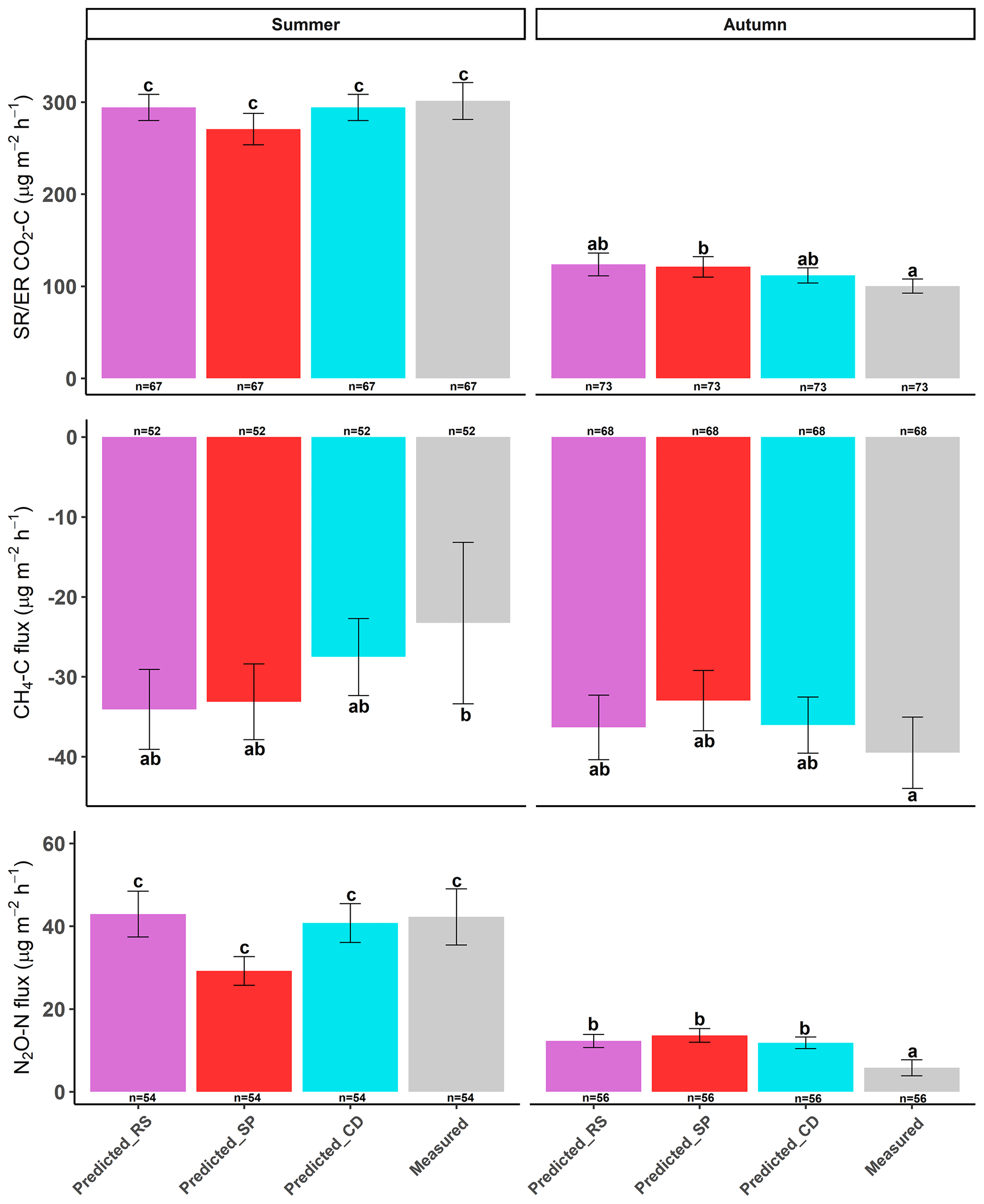
Figure A1 Bar graphs showing the mean fluxes (±SE) predicted using remote sensing (RS), soil parameters (SPs), and combined data (CD) and the measured fluxes at the sampling sites in the 30 % model test dataset. The uppercase and lowercase letters indicate significant differences (p<0.05) in the mean fluxes in the different seasons and across the measured and predicted fluxes.

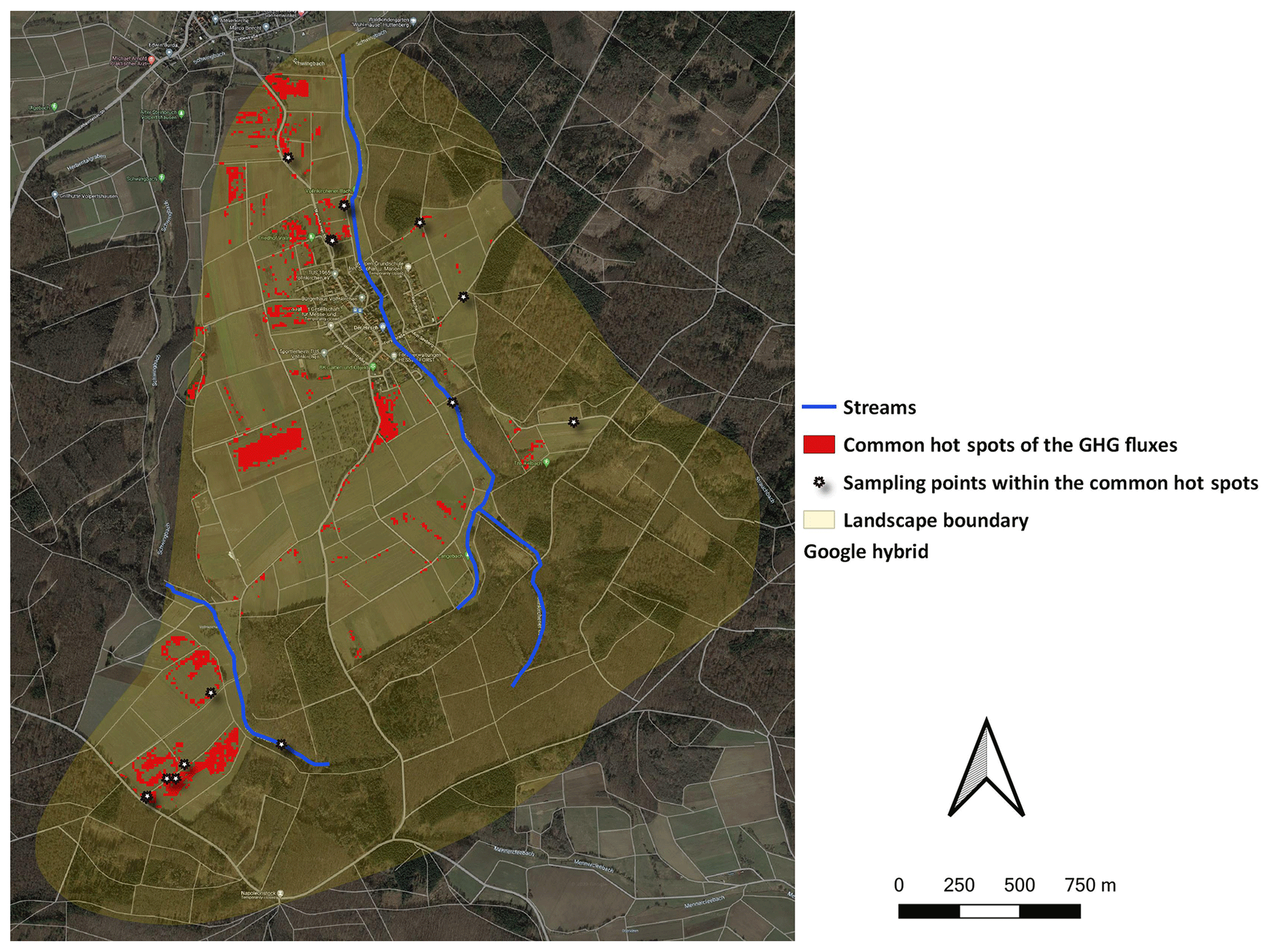
Figure A2 Map showing the common hot spot regions of the three GHG fluxes and the location of the measured sampling points within these recurrent hot spots (satellite image downloaded from © Google Maps).

Figure A3 Clover (Trifolium) on grassland ecosystems.

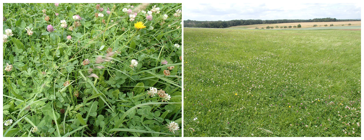
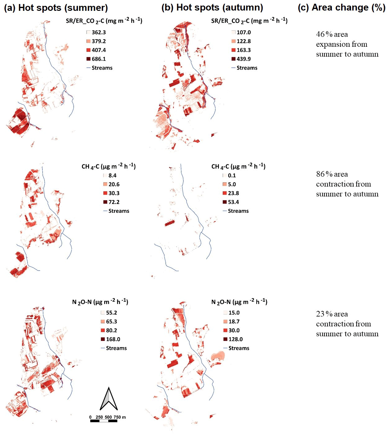
Figure A4 Maps showing the hot spots of the (a) summer and (b) autumn seasons and (c) the percentage change in the area coverage of the hot spots. These regions were defined using each season's specific hot spot threshold.

Appendix B: Tables

Table B1 Cross-validation results of different models developed for SR/ER–CO₂ fluxes in (a) forest, (b) grassland, and (c) arable land using different predictors in the training dataset. Stepwise elimination of least important predictors was implemented. The term mtry stands for the number of variables at each tree, and SOC is soil organic carbon.

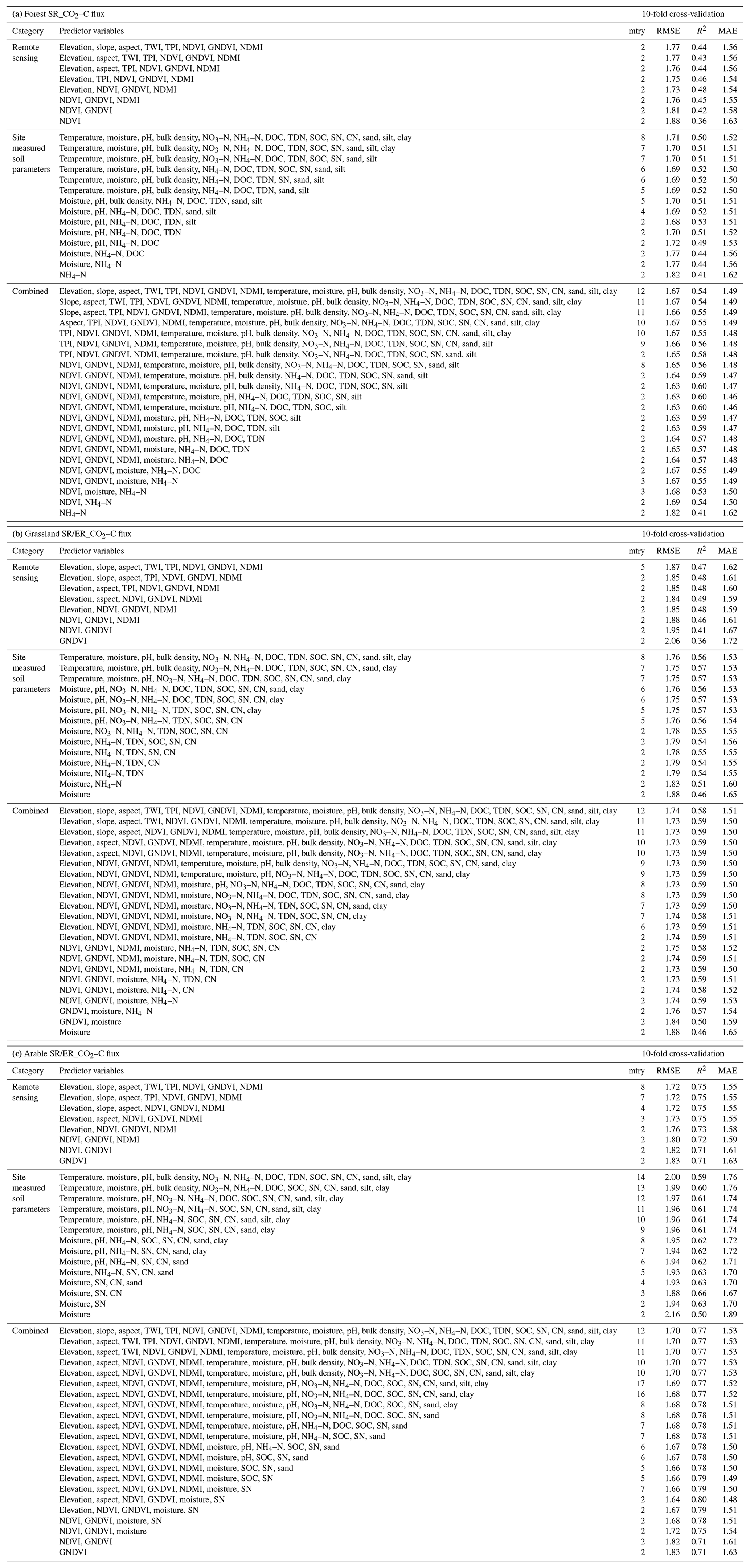
Table B2 Cross-validation results of different models developed for all (positive and negative) CH₄ fluxes in (a) forest, (b) grassland, and (c) arable land using different predictors in the training dataset. Stepwise elimination of least important predictors was implemented.

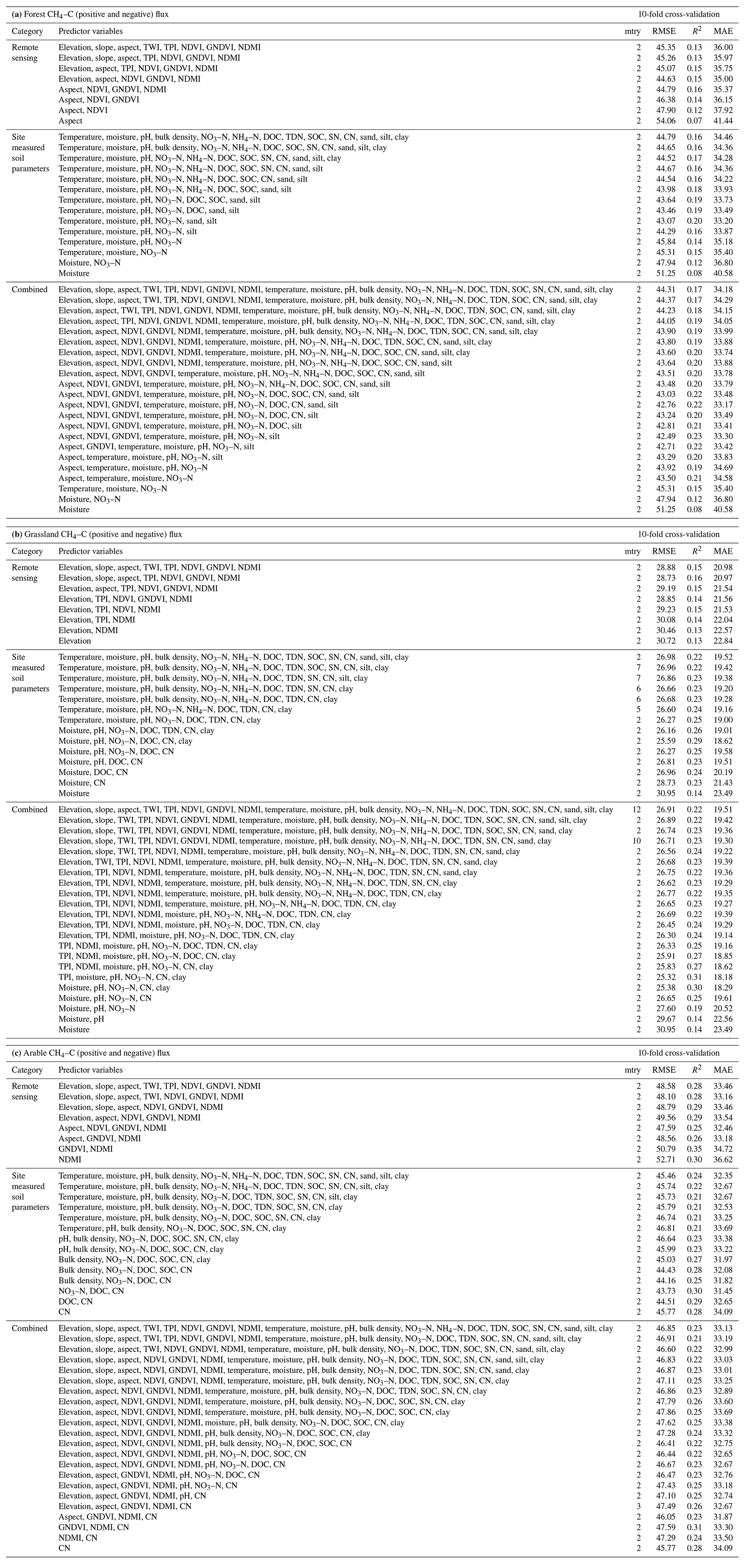
Table B3 Cross-validation results of different models developed for all (positive and negative) N₂O fluxes in (a) forest, (b) grassland, and (c) arable land using different predictors in the training dataset. Stepwise elimination of least important predictors was implemented.

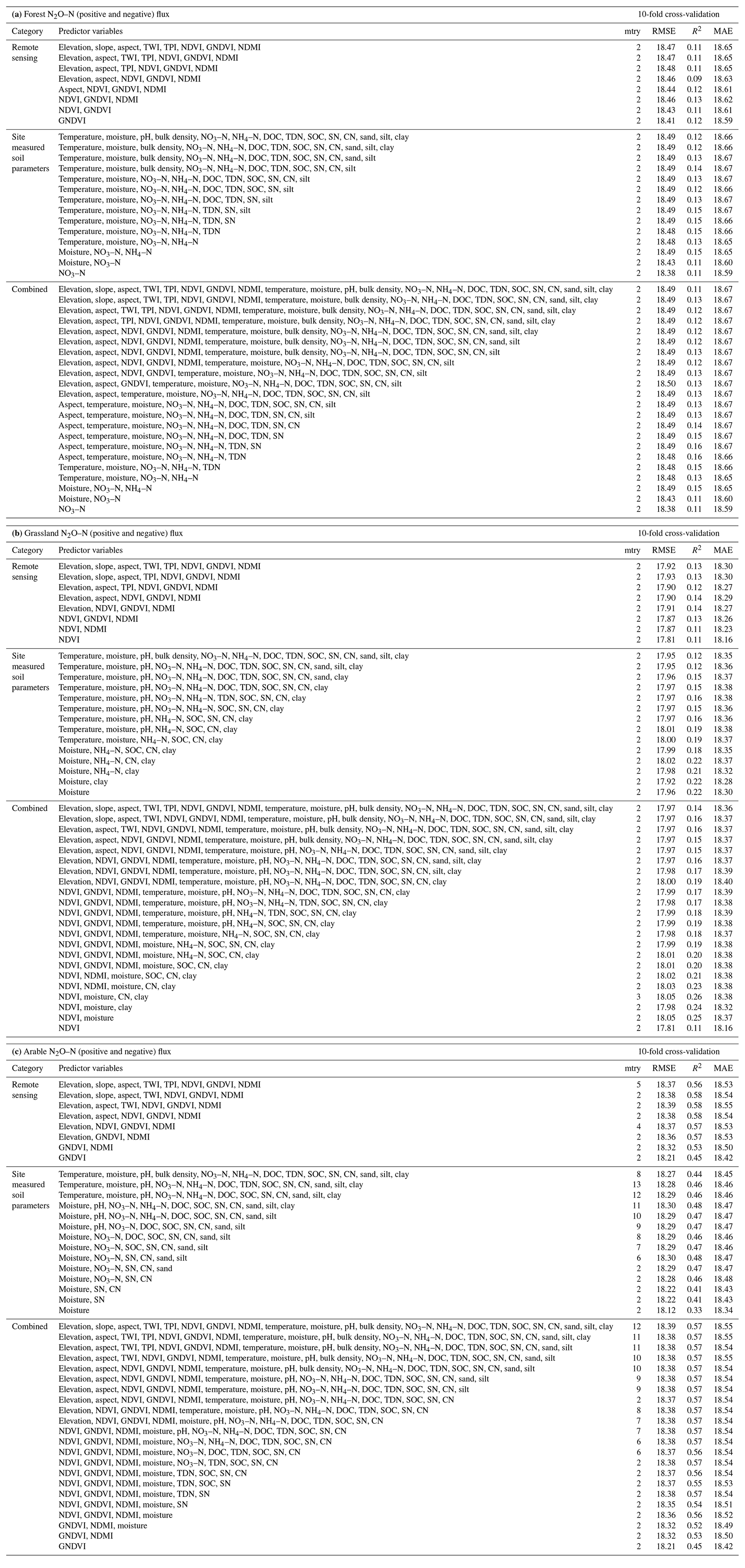
Table B4 Cross-validation results of different models developed for negative CH₄ fluxes in (a) forest, (b) grassland, and (c) arable land using different predictors in the training dataset. Stepwise elimination of least important predictors was implemented.

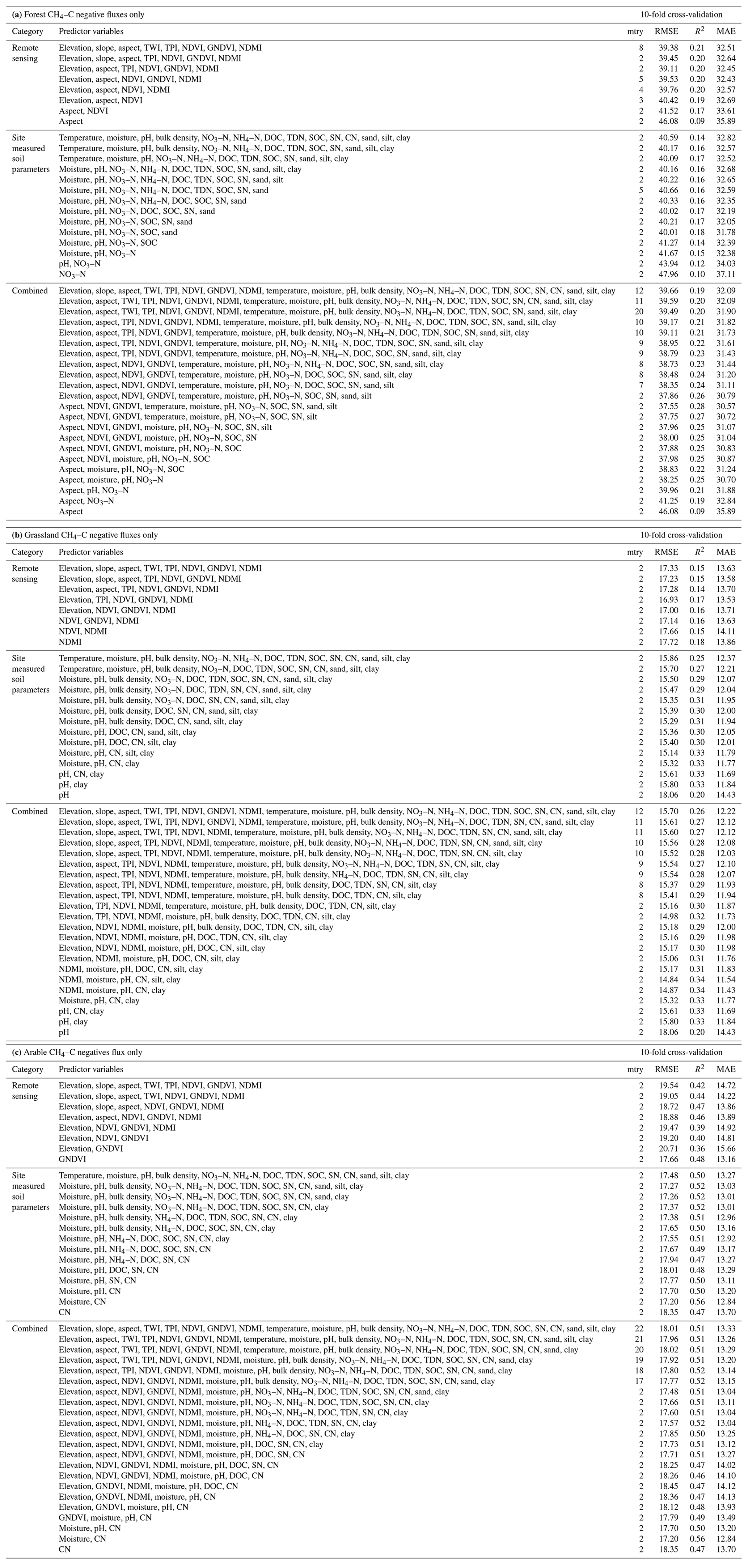
Table B5 Cross-validation results of different models developed for positive N₂O fluxes in (a) forest, (b) grassland, and (c) arable land using different predictors in the training dataset. Stepwise elimination of least important predictors was implemented.

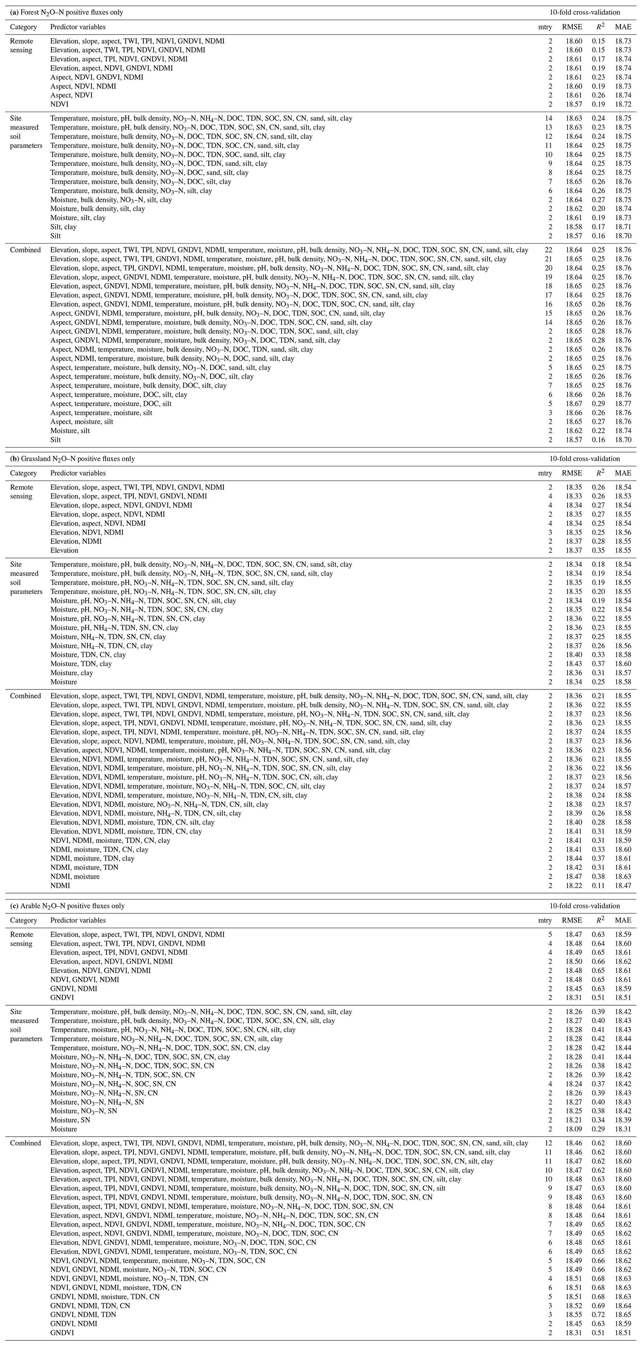
Table B6 The minimum, maximum, mean, standard deviation (SD), and standard error (SE) in the measured fluxes at all the sampling points and the predicted landscape fluxes using remote sensing (RS), soil parameters (SPs), and combined data (CD).

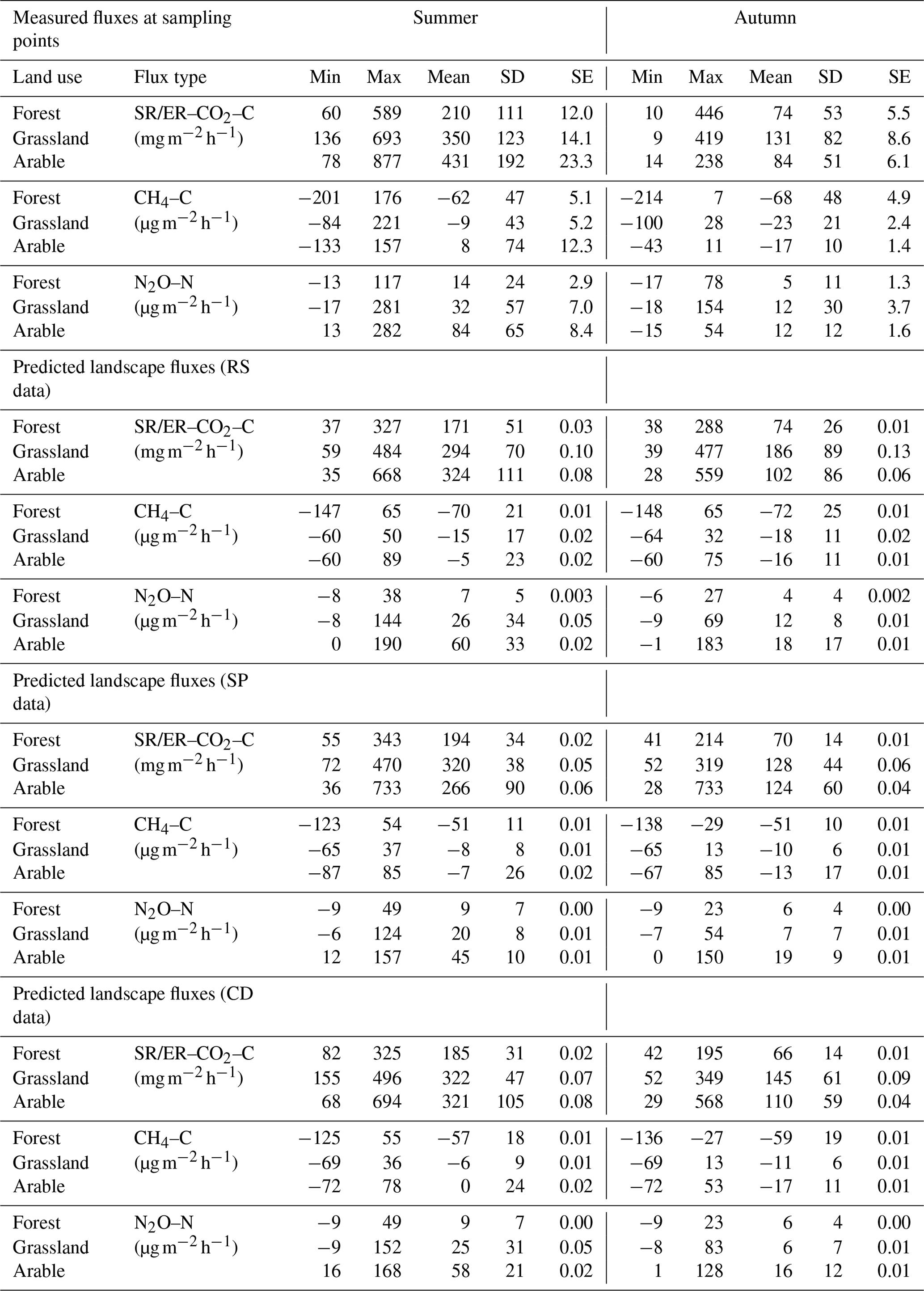
Table B7 Description of the sampling locations within the common hotspot patches of all three GHG fluxes.