the Creative Commons Attribution 4.0 License.
the Creative Commons Attribution 4.0 License.
 | 20 Dec 2023
Spatiotemporal heterogeneity in the increase in ocean acidity extremes in the northeastern Pacific
Matthias Münnich
Nicolas Gruber
The acidification of the ocean (OA) increases the frequency and intensity of ocean acidity extreme events (OAXs), but this increase is not occurring homogeneously in time and space. Here we use daily output from a hindcast simulation with a high-resolution regional ocean model coupled to a biogeochemical ecosystem model (ROMS-BEC) to investigate this heterogeneity in the progression of OAX in the upper 250 m of the northeastern Pacific from 1984 to 2019. OAXs are defined using a relative threshold approach and using a fixed baseline. Concretely, conditions are considered extreme when the hydrogen ion concentration ([H+]) exceeds the 99th percentile of its distribution in the baseline simulation where atmospheric CO2 was held at its 1979 level. Within the 36 years of our hindcast simulation, the increase in atmospheric CO2 causes a strong increase in OAX volume, duration, and intensity throughout the upper 250 m. The increases are most accentuated near the surface, with 88 % of the surface area experiencing near-permanent extreme conditions in 2019. At the same time, a larger fraction of the OAXs become undersaturated with respect to aragonite (ΩA < 1), with some regions experiencing increases up to nearly 50 % in their subsurface. There is substantial regional heterogeneity in the progression of OAX, with the fraction of OAX volume across the top 250 m increasing in the central northeastern Pacific up to 160 times, while the deeper layers of the nearshore regions experience “only” a 4-fold increase. Throughout the upper 50 m of the northeastern Pacific, OAXs increase relatively linearly with time, but sudden rapid increases in yearly extreme days are simulated to occur in the thermocline of the far offshore regions of the central northeastern Pacific. These differences largely emerge from the spatial heterogeneity in the local [H+] variability. The limited offshore reach of offshore-propagating mesoscale eddies, which are an important driver of subsurface OAX in the northeastern Pacific, causes a sharp transition in the increase in OAX between the rather variable thermocline waters of nearshore regions and the very invariant waters of the central northeastern Pacific. The spatially and temporal heterogeneous increases in OAX, including the abrupt appearance of near-permanent extremes, likely have negative effects on the ability of marine organisms to adapt to the progression of OA and its associated extremes.
- Article
(8355 KB) - Full-text XML
- BibTeX
- EndNote


Ocean uptake of anthropogenic carbon dioxide (CO2) from the atmosphere is the main driver of the ongoing surface ocean acidification (OA), i.e., the long-term increase in the hydrogen ion concentration [H+] and the decreases in pH (with pH = ) and aragonite saturation state (ΩA) in the surface ocean (Hoegh-Guldberg et al., 2018; Bindoff et al., 2019; Doney et al., 2009; Caldeira and Wickett, 2003). These trends are bound to increase the occurrence of ocean acidity extreme events (OAXs). But how such extremes progress and what this means in terms of their average duration, frequency, and intensity has only been analyzed by a handful of model-based studies so far (Gruber et al., 2021; Burger et al., 2020; Hauri et al., 2013a; Negrete-García et al., 2019), primarily due to the lack of long and high-spatiotemporal-resolution observational records of ocean carbonate chemistry variables.
OAXs are defined as either rare and unusually high (low) in [H+] (pH, ΩA) events (Desmet et al., 2022; Gruber et al., 2021; Burger et al., 2020, 2022) or events when the [H+] concentration (pH, ΩA) is above (below) a given absolute threshold known to be harmful to certain marine organisms (Hauri et al., 2013a). The rareness of events is usually determined by requiring events to cross a “extreme” relative threshold, often determined from a certain percentile (e.g., 1st or 99th) of a cumulative frequency distribution (Seneviratne et al., 2012; Gruber et al., 2021). The frequency distribution itself is obtained by sampling the environmental conditions over a certain baseline period (Oliver et al., 2021). Irrespective of the choice of absolute or relative thresholds to identify extremes, all studies conducted so far have confirmed that OAXs have become already more frequent, longer, and more intense since the preindustrial era and that these trends will continue in the future (Burger et al., 2020; Gruber et al., 2021; Hauri et al., 2013a). They have also confirmed that the main driver of these changes is the increase in atmospheric CO2 driving an increase in the surface ocean concentration of anthropogenic CO2. For example, between the preindustrial period and recent decades, the number of surface extreme days for [H+] across the global surface ocean was shown to increase from ∼ 4 to ∼ 300 d a year for OAX defined using a relative threshold on a fixed preindustrial baseline (Burger et al., 2020). A similar increase was simulated at 200 m depth. While this global-scale increase is very large, it was found to occur relatively smoothly in time (Burger et al., 2020; Gruber et al., 2021). However, this might not be the case at the regional scale, where variability is larger. So far, limited emphasis has been given to such potential spatial and temporal heterogeneities in the progression of OAX and the potential for abrupt changes. This is in part a consequence of the fact that the global studies used relatively coarse-resolution Earth system models, which do not resolve mesoscale variability that has been shown to be rather relevant for generating OAX (Desmet et al., 2022).
In fact, such abrupt changes in OAX have been detected at the regional scale in the California and Humboldt current systems (Hauri et al., 2013a; Franco et al., 2018) and in the Southern Ocean (Hauri et al., 2015; Negrete-García et al., 2019). These OAXs, defined in these studies as undersaturation events where ΩA < 1, exhibit abrupt onsets, nonlinear increases, and sudden shoalings. For example, in the nearshore bottom waters off California, Hauri et al. (2013a) showed that while the median duration of such undersaturation events increased only modestly up to the year 2000, these events abruptly become near permanent in the ensuing decades. Such abrupt increase may also occur for OAX defined using relative thresholds, i.e., when the environmental conditions suddenly shift to conditions outside the previously established variability ranges. Such an abrupt increase in OAX could have especially deleterious effects on marine organisms since they are not only exposed to conditions that are outside the variability that they are adapted to (Vargas et al., 2017, 2022; Kroeker et al., 2020; Rivest et al., 2017; Cornwall et al., 2020) but are also forced to transition to the new conditions at a speed that likely exceeds their capacity to adapt (Gruber et al., 2021).
The rate and potential abruptness of the increase in OAX in response to the rise in atmospheric CO2 is likely to vary between regions and depths owing to differences in the rate of change in the underlying variables of the marine carbonate system (Ma et al., 2023) and because of differences in the magnitude and type of variability in these variables (Sutton et al., 2019; Carter et al., 2019; Keller et al., 2014). Owing to the generally Gaussian-type distribution of environmental conditions, the same shifts in the underlying distribution impact extremes very differently in high-variability versus low-variability regions. We generally expect that regions characterized by large variability tend to experience smaller increases in OAX than regions with low variability. The same underlying concept is captured by the time of emergence (ToE) concept, which is the time for the trend in OA to exceed the background variability (Sutton et al., 2019; Turk et al., 2019; Carter et al., 2019; Keller et al., 2014). This means that after the ToE has passed, the change is clearly detectable and the conditions are, on average, very different from anything in the past. Thus, the ToE in open-ocean sites that are characterized by low variability tend to be much shorter than those in coastal sites, where variability is high (Sutton et al., 2019; Turk et al., 2019; Carter et al., 2019; Keller et al., 2014). This also means that we expect the largest changes in OAX in the open-ocean regions characterized by low variability. For abruptness, the relationship with variability is not so clear, since this metric strongly depends on the details of the variability and of the nature of the underlying change in the marine carbonate system variable of interest. Still, low-variability regions might be more prone to abrupt changes than those characterized by high variability.
Of particular relevance with respect to OAX is the northeastern Pacific, due to its vulnerability to OA. Waters naturally low in pH and ΩA make up the upper 250 m depth, particularly inshore along the Alaskan, Canadian, and US west coasts where the saturation horizon with regard to aragonite is naturally shallow (Jiang et al., 2015; Byrne et al., 2010; Feely and Chen, 1982; Feely et al., 2008). Besides, observation and model-based studies found rapid acidification in those regions (Jiang et al., 2019; Gruber et al., 2012; Hauri et al., 2013b; Turi et al., 2016), threatening important marine ecosystems and their services since the region hosts highly productive waters and important fisheries, including OA-sensitive species (Mundy, 2005; Messié et al., 2009; Pauly and Christensen, 1995; Bednaršek et al., 2014, 2017, 2020; Long et al., 2016; Swiney et al., 2016; Williams et al., 2019).
Spatial patterns and regional drivers of OAX in the northeastern Pacific have been investigated recently in a regional ocean model that explicitly resolves mesoscale variability (Desmet et al., 2022). Within the upper 100 m, westward-propagating mesoscale cyclonic eddies were found to drive the largest and longest-tracked OAX, defined as combined unusually low-pH ΩA space-time events, revealing the key role of mesoscale variability in OAX formation and sustenance. Hence, in the California Current System (CCS), as well as hundreds of kilometers offshore, OAXs are shaped by the extensive mesoscale activity of the CCS (Desmet et al., 2022; Zhao et al., 2021; Chabert et al., 2021; Combes et al., 2013; Nagai et al., 2015; Amos et al., 2019; Chenillat et al., 2016). Near the US west coast, shallow and intense OAXs emerge from seasonal upwelling, which confers high pH and ΩA natural variability to the waters (Desmet et al., 2022; Fassbender et al., 2011, 2018; Turi et al., 2014). Therefore, leading drivers of OAX in the northeastern Pacific differ across space, with different scales of variability predominating, likely to drive a spatially heterogeneous temporal progression of OAX in response to the rise in atmospheric CO2.
In the present study, we quantify the rate, the abruptness, and the heterogeneity of the increase in OAX across the upper ocean of the northeastern Pacific. We thereby use a high-resolution mesoscale-resolving oceanic model, focus on the period from 1984 through 2019, and adopt a relative threshold definition of the OAX on the basis of the [H+] concentration. We also attribute which fraction of the change is due to the rise in atmospheric CO2.
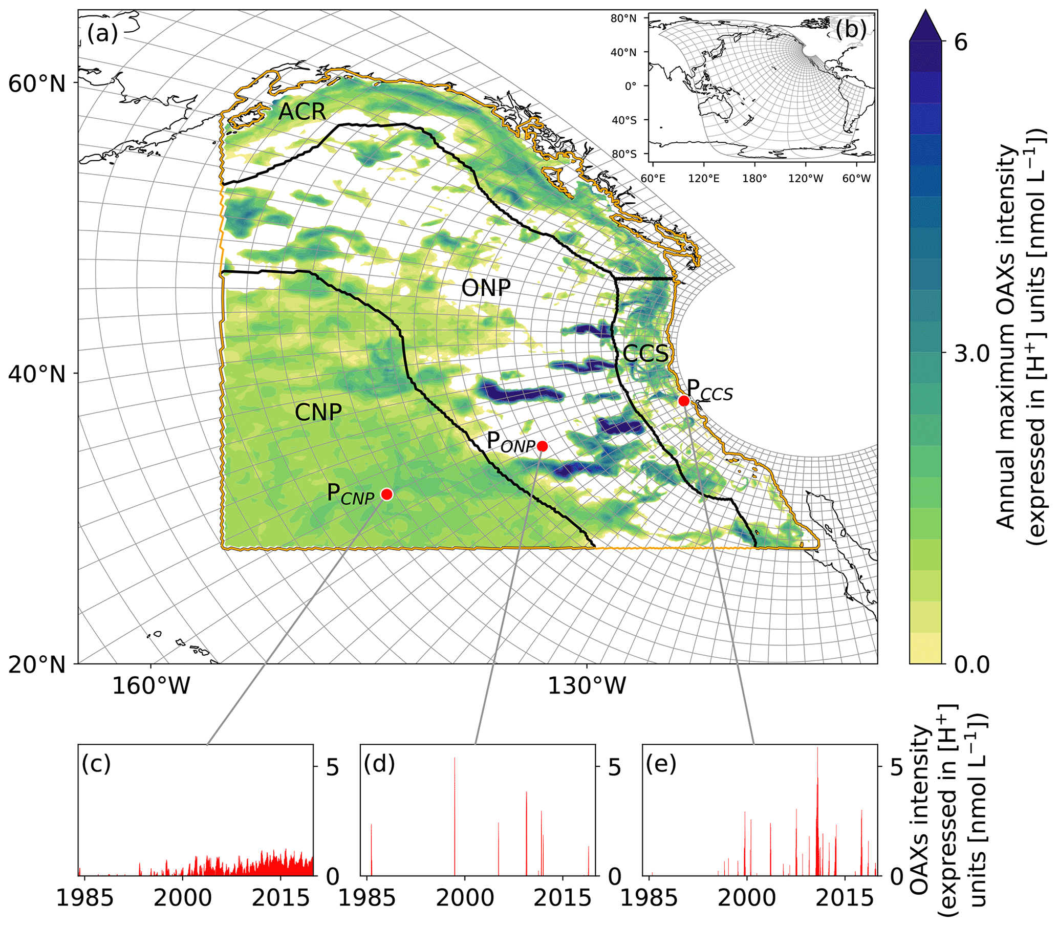
Figure 1Map of the analysis domain, the selected subregions, and key properties of the diagnosed OAX. (a) Map of the northeastern Pacific with the telescopic grid of the model plotted in grey for every 10th grid cell. The black contours delimit the four selected subregions, i.e., the two coastal regions inshore of 300 km, namely the Alaskan Coastal Region (ACR) and the California Current System (CCS), and the two open-ocean regions, i.e., the offshore northeastern Pacific (ONP) and the central northeastern Pacific (CNP) regions. The domain of analysis is denoted by the orange contour line. The annual maximum intensity of the simulated OAXs in year 2014 at 100 m depth is plotted on top. White regions indicate that no OAX occurred in that year at this depth. (b) Map of the whole ROMS-BEC telescopic grid, plotted for every 20th grid cell. (c–e) Time series of [H+] intensity at 100 m depth at the three locations depicted by red points in (a), i.e., (c) PCNP in the CNP region (31.66∘ N, 143.77∘ W), (d) PONP in the ONP region (34.97∘ N, 133.07∘ W), and (e) PCCS in the CCS (38.08∘ N, 123.32∘ W).
2.1 Simulations
This study is based on the UCLA-ETH version of the Regional Oceanic Modeling System (ROMS) (Shchepetkin and McWilliams, 2005) coupled to the biogeochemical ecosystem model (BEC) (Frischknecht et al., 2018; Moore et al., 2013). We use the same model configuration and forcing as described by Desmet et al. (2022), and we refer the reader to that study for further details. An important feature of our model configuration is the telescopic grid that resolves mesoscale features across a substantial fraction of the northeastern Pacific with highest grid refinement near the US west coast pole of the grid (Fig. 1b). At the same time, the model simulates the circulation of the entire Pacific, avoiding the need to provide lateral boundary conditions except at a few places in the Southern Ocean, i.e., more than 9000 km away from the analysis domain.
We run two simulations with different carbon forcings. The first one corresponds to the simulation used by Desmet et al. (2022) and consists of a hindcast simulation (HCast) from 1979 through 2019, where atmospheric pCO2 is prescribed to increase according to observations (Landschützer et al., 2020), and where the dissolved inorganic carbon (DIC) concentration at the lateral southern open boundary of the model is transient but does not include interannual variability. Our HCast simulation uses slightly different initial conditions than employed by Desmet et al. (2022) as a result of a change in the forcing used for the model spinup. While Desmet et al. (2022) used daily fields from the year 1979 as the forcing for the spinup, we use a normal-year forcing (apart from atmospheric CO2, which is transient). The normal-year forcing is created by adding daily anomalies of the year 2001 to the climatological mean surface fields of wind stress, shortwave and longwave radiation, and freshwater fluxes derived from ERA-5 (Hersbach et al., 2020; Copernicus Climate Change Service (C3S), 2017). The second simulation is a control simulation (CCons), where we kept the long-term mean atmospheric pCO2 and DIC concentration at the lateral southern boundary at the 1979 levels by linearly detrending them. This simulation was also run for the years 1979 through 2019. We discard the first 5 years and then use daily mean outputs from 1984 to 2019 for both simulations for our analysis of the extreme events. The hydrogen ion concentration ([H+], at the total scale) and the saturation state of aragonite (ΩA) are computed offline using the MOCSY 2.0 routine as described in Desmet et al. (2022).
We divide the northeastern Pacific region (28–62∘ N, 105–155∘ W) into a total of four regions (Fig. 1a). Two are coastal regions extending up to 300 km off the coast, namely the CCS (28–46.5∘ N) and the Alaskan Coastal Region (ACR; north of 46.5∘ N). The choice of 300 km reflects, on the one hand, the average width of the nearshore band of high particulate organic carbon concentrations (Amos et al., 2019) and, on the other hand, the boundary inshore of which the majority of westward-propagating mesoscale eddies tend to form (Nagai et al., 2015; Chenillat et al., 2016; Amos et al., 2019). The other two regions are open-ocean regions, with the first one denoted as the “offshore northeastern Pacific” (ONP), impacted by mesoscale eddies that originate from the nearshore regions and propagate all the way into this open-ocean region. The second is the central northeastern Pacific (CNP) that shows no evidence of this coastal imprint. We delineate the ONP and CNP regions by computing the eddy fronts at 100 and 200 m, respectively, and then taking the average of the two (see Sect. 2.4 below for further details).
2.2 Model evaluation
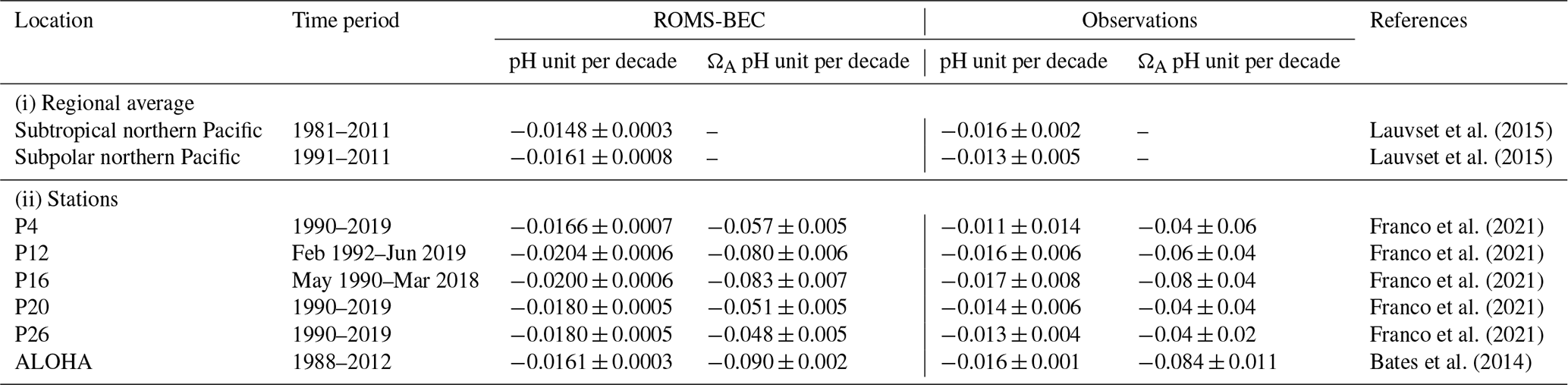
A thorough evaluation of the climatological distribution of key physical and carbon variables simulated in the HCast was provided by Desmet et al. (2022). This evaluation, as well as that of the simulated daily surface variability, gave excellent results, except for a tendency of the model to produce too low pH and ΩA levels in the thermocline of the CCS. Although our HCast simulation is not numerically equivalent to the simulation employed by Desmet et al. (2022) owing to the different initial conditions (cf. Sect. 2.1), they present very similar evaluation results (not shown). Here we further evaluate the surface OA trends in pH and ΩA of the model against observations (Table 1).
We first evaluate regionally averaged surface pH trends in the northern Pacific against trends derived from SOCATv2 data (Lauvset et al., 2015) (Table 1). For better comparison, we spatially average surface pH over the biomes used in Lauvset et al. (2015) and then compute the linear trend on the spatially averaged time series. The modeled surface pH in the subtropical northern Pacific decreases by 0.015 per decade from 1981 to 2011, which is within the range of the observed trend of −0.016 ± 0.002 per decade (Lauvset et al., 2015). The model's trend of −0.016 pH unit per decade from 1991 to 2011 in the subpolar northern Pacific, although overestimated compared to observations, is also within the range of the observed trend of −0.013 ± 0.005 per decade (Lauvset et al., 2015).
We additionally evaluate our model-simulated pH and ΩA surface trends against time series data collected at station ALOHA (Bates et al., 2014), as well as against the line P time series (Franco et al., 2021). All the simulated trends are within the range of observed trends, except the pH trend at station P26 (Table 1). The average modeled surface pH (ΩA) trend across the five line P stations is −0.019 per decade (−0.06 per decade) against −0.014 per decade (−0.05 per decade) in Franco et al. (2021).
Lauvset et al. (2015)Lauvset et al. (2015)Franco et al. (2021)Franco et al. (2021)Franco et al. (2021)Franco et al. (2021)Franco et al. (2021)Bates et al. (2014)Table 1Linear trends in pH and ΩA (per decade) for the two northern Pacific biomes used in Lauvset et al. (2015) (subtropical and subpolar) and six stations (line P stations and ALOHA; see Appendix Fig. B1). Given are the modeled and observed trends, together with their 2 standard deviation credible intervals (95 % CrI).
While the evaluation of subsurface pH and ΩA trends is not yet possible given the lack of long-term time series observations, we evaluate the simulated subsurface trends in DIC down to about 300 m depth against observations derived from the line P time series (Appendix Fig. B2; Franco et al., 2021). The simulated DIC trends (DIC is normalized to a salinity of 33 psu) in the subsurface of line P stations are in the range of observed trends (Appendix Fig. B2). However, the model tends to have larger trends than suggested by the observations. In intermediate waters (150–300 m depth), simulated DIC trends are 2 % larger than the upper bound of observed trends in open-ocean stations and 15 % larger in the coastal station P4 (Appendix Fig. B2). We further discuss the implications of this discrepancy in Sect. 4.4.
Overall, although subsurface trends in DIC tend to be overestimated, our model simulates pH and ΩA surface trends within the range of the trends that have been observed during the last 4 decades, giving us confidence in the analysis of the progression of acidity extreme events.
2.3 Ocean acidity extremes (OAX)
We define ocean acidity extreme events (OAXs) as temporally connected grid cells, for which [H+] exceeds the 99th percentile of temporally aggregated daily [H+] from 1984 to 2019 at a given location (similar to in Gruber et al., 2021). To determine the 99th percentile threshold, we used the CCons simulation where the long-term mean atmospheric CO2 was kept at the 1979 levels. In other words, we used a fixed baseline approach where the initial conditions of the late 1970s were used as the reference period. This choice of a reference period is somewhat arbitrary, but the late 1970s–early 1980s represent for many oceanographic parameters the first period for which we have global-scale observation-based estimates (see, e.g., Ma et al., 2023). This temporally fixed threshold was then used to detect OAXs in both the CCons and HCast simulations. We focus our analysis on OAX occurring in the upper 250 m of the water column.
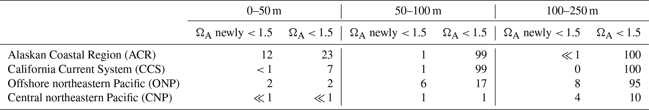
We derive three local metrics, namely (i) yearly extreme days (in d; number of days per year above the 99th percentile of [H+]), (ii) annual mean event duration (in d; the average number of consecutive days above the 99th percentile of single events within a year) and (iii) annual maximum intensity (in nmol L−1; maximum [H+] anomaly with respect to the percentile threshold). These metrics are computed at three depths, i.e., the surface layer in direct interaction with the atmosphere and two subsurface layers, namely 100 m, corresponding to the transition from the euphotic zone to the twilight zone, and 200 m, corresponding to the upper thermocline. Note that while the truncation of extremes between years alters the results for duration, it allows for the calculation of annual extreme-event characteristics. We additionally derive an integrative metric, namely the annual mean volume fraction of OAX (in %; the average fraction of the daily volume of grid cells with [H+] above the 99th percentile relative to the total volume extending from 0 to 250 m depth), computed separately for each of the four regions of the northeastern Pacific depicted in Fig. 1a (ACR, CCS, ONP and CNP) and three depth bins (0–50 m, 50–100 and 100–250 m). Additionally, we compute in each of these regions the fraction of the volume of the [H+] extremes that is undersaturated with regard to aragonite (ΩA < 1) at the time of the extreme. Within the OAX with undersaturated conditions, we further identify those that are supersaturated (ΩA ≥ 1) in the CCons simulation. We refer to this last fraction as the fraction of newly undersaturated OAXs.
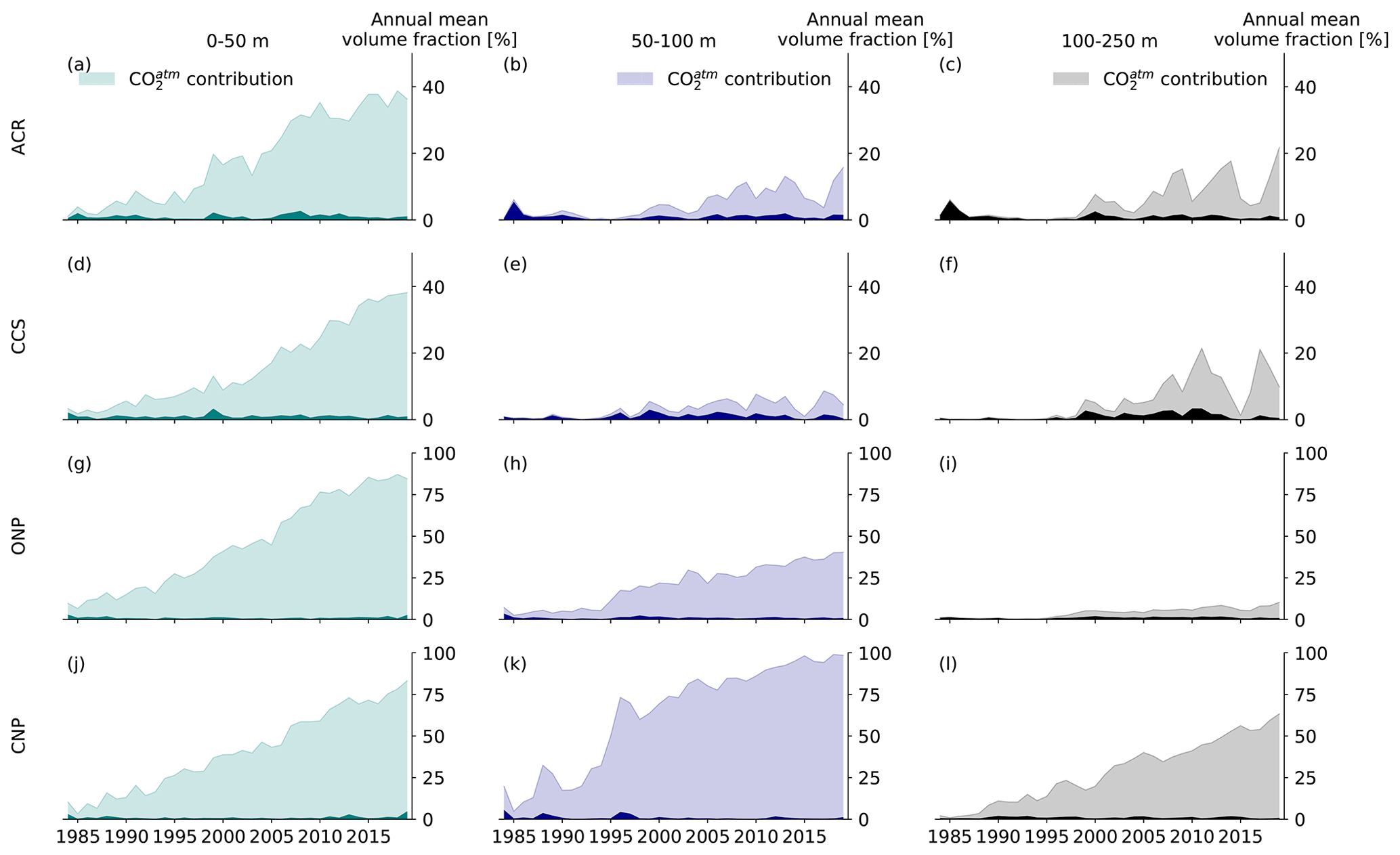
Figure 2Time series of the annual mean volume fraction characterized by [H+] extremes (OAX) for the four different regions of the northeastern Pacific shown in Fig. 1a (rows) and three different depth sections (from left to right: 0–50, 50–100, and 100–250 m depth). Dark and light colors depict the OAX volume fraction in the CCons and HCast scenario, respectively, with the difference between the two denoting the contribution of the rise in atmospheric CO2 to the OAX volume fraction from the HCast scenario (CO contribution, hatched area). Note the different scales of the top two rows (0 %–50 %) and bottom two rows (0 %–100 %).
2.4 Return periods, time of emergence (ToE), and eddy front
We characterize the return periods of different [H+] intensity levels using the generalized extreme value distribution G (Coles, 2001):
where μ, σ, and ξ are the location, scale, and shape parameters, respectively. We extract the annual maxima [H+] at each grid cell and fit G to the annual maximum data for the 1984–1998 and 2005–2019 periods, respectively, using the stats.genextreme function from SciPy. We then compute at each location the return periods (in years) for 24 discrete return intensity levels ranging from 0.05 to 6 nmol L−1. We focus on return periods shorter than a century and set all longer return periods to 200 years prior to computing the spatial median and 40th and 60th percentile return periods within the ACR, CCS, ONP, and CNP regions at the surface and at 100 and 200 m depth. The method is found to be robust to the number of data points to which G is fitted, i.e., 15 data points for each period in our study, given the small standard deviation (1.4 years) of the return periods computed for the CCons scenario on 15, 20, and 25 years (respectively 15, 20, and 25 data points; Appendix Fig. B3).
We compute the time of emergence (ToE) as a measure of the time it takes for the linear long-term trend signal to exceed the 99th percentile threshold used to detect OAX. We first compute at each individual grid cell a linear regression from the daily [H+] data from 1984 through 2019 from the HCast scenario, assuming the trend signal to be linear over this period. We then calculate the number of years after 1979 when this linear trend exceeds the 99th percentile threshold computed from the CCons scenario daily data from 1984 to 2019. This is done at each location at the surface and at 100 and 200 m depths. We refer to as “near-permanent OAX” when emergence has occurred, i.e., when the linear long-term trend signal has exceeded the 99th percentile threshold used to detect OAX.
At both 100 and 200 m depth we define an eddy front based on the westward extent of detected eddy-driven OAXs in Desmet et al. (2022). This eddy front measures the farthest distance from the coast at which eddy-induced variability significantly alters the [H+] threshold (99th) value in our simulation. Such alteration occurs when eddy-induced variability accounts for more than 1 % of the time period at a given location, in which case the threshold depends on the [H+] carried by mesoscale eddies rather than background variations at that location (Appendix Fig. A1). Further offshore of this front, the threshold of the offshore regime is not affected anymore by the mesoscale imprint of nearshore conditions. Detailed methodology on the calculation of the depth-dependent eddy front can be found in Appendix A.
Table 2Fraction (in %) of the OAX volume that is characterized by undersaturated conditions with regard to aragonite averaged over 1984–2019 for the four different regions of the northeastern Pacific shown in Fig. 1a and for three different depth layers. Numbers in the “ΩA newly < 1” column give the fraction of the OAX volume that is newly undersaturated with regard to aragonite. This is computed by identifying the fraction of the OAX volume that is undersaturated in the HCast simulation but supersaturated in the CCons simulation where atmospheric CO2 was kept at its 1979 value.

3.1 Progression of OAX in the northeastern Pacific
Between 1984 and 2019, the annual mean volume fraction characterized by extreme [H+] conditions (OAX) in the upper 250 m increases manifold, yet spatially varied across the northeastern Pacific (Fig. 2). In the upper 50 m, this volume fraction increases from a few percent in the early 1980s to around 40 % in the two coastal regions (Fig. 2a and d) and to about 85 % in the open-ocean regions (Fig. 2g and j), representing a between 8- and 15-fold increase over the 36 years of our simulation. In the 50–100 m depth range, the regional differences are even larger. While the central northeastern Pacific (CNP) approaches permanent extreme conditions (OAX volume fraction > 95 % on average during the last 5 years), the other regions experience a more modest increase (Fig. 2b, e, h, and k). This strong regional difference persists in the 100–250 m depth range, with the CNP region experiencing an increase to a volume fraction of OAX of more than 50 %, while the volume fraction in the adjacent ONP open-ocean region increases to only about 10 %, similar to the changes seen in the two coastal regions (Fig. 2c, f, i, and l). Furthermore, the temporal progression differs across regions. The increase is mainly linear in the surface layer, while the subsurface (i.e., below 50 m depth) experiences more abrupt transitions and stronger year-to-year variability. Striking is the step increase in OAX in the subsurface layers of the two coastal regions around the year 1995 (Fig. 2b, c, e, and f). This is also seen in the open-ocean regions (Fig. 2h and k). The strongest year-to-year variability is found in the 100–250 m range of the two coastal regions, with a near collapse of the OAX volume fraction in the CCS and ACR in 2015, concomitant with the strong 2014/16 El Niño (Fig. 2c and f).
Many of the OAX below the top 50 m, and especially those in the coastal regions, are also characterized by undersaturated (corrosive) conditions with regard to the CaCO3 mineral aragonite, i.e., have ΩA < 1 (Table 2). This joint stress from extremely low pH and corrosive conditions is expected to be particularly harmful for ocean organisms that form shells out of aragonite such as pteropods (Bednaršek et al., 2014; Feely et al., 2018). While such corrosive conditions in OAX are rare in the upper 50 m of the ocean, between 66 % and 100 % of the OAX events are corrosive below 50 m in the two coastal regions. Also in the ONP below 100 m, the majority (60 %) of the OAX have such corrosive conditions (Table 2). While the majority of these events would have been corrosive even in the absence of any increase in atmospheric CO2 in the 100 to 250 m depth layer, about an eighth (CCS) to a third (ACR) of the corrosive OAX between 50 and 100 m depth in the two coastal regions has become corrosive over the course of the 41 years of our simulation (Table 2). There, 10 % and 21 %, respectively, of the volume of OAX has become undersaturated, while these waters would have stayed supersaturated without the increase in atmospheric CO2. In contrast to the subsurface waters in the ACR, CCS, and ONP regions, the OAX in the subsurface waters of the CNP remain supersaturated.
These differences in corrosiveness of the OAX reflect the distribution of the climatological saturation horizon (depth level where ΩA = 1) and how this horizon shoals in response to the invasion of anthropogenic CO2. With the atmospheric CO2 kept at the 1979 level, this horizon sits below 300 m in the CNP and ONP regions but shoals to less than 60 m in the nearshore coastal regions. Still, the saturation horizon sits below 100 m in more than 80 % of the coastal areas (Appendix Fig. B4). With the increase in atmospheric CO2, this horizon shoals by 45 m on average in coastal areas, bringing the saturation horizon into the top 100 m, leading to many additional corrosive OAX.
3.2 Role of rise in atmospheric CO2
The strong increase in the OAX with time is almost entirely attributable to the increase in atmospheric CO2 ( contribution in Fig. 2). If atmospheric CO2 was held at the 1979 levels, the volume of OAX would have exhibited no significant trend (dark-colored areas) but only would have fluctuated from year-to-year at a level of a few percent in all regions and depth layers. Concretely, depending on the depth layer and region, the fraction of the volume occupied by OAXs in the last 15 years of the hindcast is 4- to 160-fold larger than in the CCons simulation, where atmospheric CO2 did not increase (Fig. 2).

Figure 3OAX characteristics as a function of atmospheric CO2 between 1984 and 2019 in the (a–c) two coastal and (d–f) two open-ocean regions of the northeastern Pacific analysis domain. (a, d) Annual mean OAX volume fraction in three different depth layers (0–50, 50–100, and 100–250 m depth). (b, e) Annual mean event duration (d) and (c, f) annual maximum intensity (nmol L−1) at surface (cyan), 100 m (dark blue), and 200 m (black) depth. In all panels, the simulated OAX characteristics are plotted against the yearly averaged atmospheric pCO2 over the northeastern Pacific domain. Corresponding years are indicated at the top. Linear regressions (r2>0.7) are plotted in each panel, and the associated rates of increase (µatm−1) are given.
In order to assess the impact of the rise in atmospheric CO2 in more detail and to also diagnose its impact on the duration and the annual maximum intensity of the OAX, we analyze these metrics as a function of atmospheric CO2 rather than as a function of time (Fig. 3). This permits us to scale the various metrics as a function of the main driver of change. We thereby combine the two coastal and two open-ocean regions.
On average across the entire northeastern Pacific, OAXs occupy an additional 6.3 % of the upper 250 m depth, last 10.2 d longer, and are 0.16 nmol L−1 (≈ −0.006 pH units) more intense for every additional 10 µatm of CO2 in the atmosphere. Near the surface, the increase in OAX volume fraction linearly follows the atmospheric CO2 rise in both coastal and open-ocean regions (r2>0.96), with a rate of change in the open-ocean regions that is twice as large as that in the coastal regions, i.e., 1.3 % versus 0.6 % µatm−1 (Fig. 3a and d). The increase rate decreases substantially below 50 m in the coastal regions (Fig. 3a) and below 100 m depth in the open-ocean regions (Fig. 3d). Between 50 and 100 m depth, the offshore OAX volume fraction abruptly increases at about 355 µatm, corresponding to the early step increase in Fig. 2h and k.
Similar near-linear relationships with the rise in atmospheric CO2 are found for the annual mean duration (Fig. 3b and e) and for the annual maximum intensity of the OAX (Fig. 3c and f). In the coastal regions, the duration increases twice as fast at the surface as in the subsurface (0.59 and 0.21 d µatm−1, respectively; Fig. 3b). While the annual mean duration of OAX at the surface is ∼ 7 d under atmospheric CO2 levels of 1984–1998 (∼ 351 µatm), it is nearly 4 times longer, i.e., about 30 d under atmospheric pCO2 levels of 2005–2019 (∼ 390 µatm). At depth, the lower rate of increase leads to durations toward the end of the simulations of around 10 d (Fig. 3b).
In the open-ocean regions, the durations of the OAX are much longer than in the coastal regions and also increase faster (Fig. 3e). At the surface, the rate of increase is 3 times larger than in the coastal regions (∼ 1.58 d µatm−1), increasing the duration of an [H+] extreme from ∼ 16 d in the first 15 years of the hindcast to more than 75 d in the last 15 years. The rate of increase in the open-ocean regions is largest at 100 m, being about 50 % larger than that at the surface and more than twice as large as at 200 m.
The annual maximum intensity of OAX also increases with increasing atmospheric CO2 throughout the northeastern Pacific, but in contrast to the other metrics there are fewer differences between regions and between different depths (Fig. 3c and f). In the coastal regions, the maximum intensity doubles at the surface between 1984–1998 and 2005–2019, increasing from values around 0.5 nmol L−1 to more than 1 nmol L−1. This equates to an oceanic pH change of about −0.022. Down to 100 m depth in coastal regions and in the surface of open-ocean regions, the intensities increase at nearly the same rate as those simulated at the surface of coastal regions. At 200 m depth and in the subsurface of open ocean regions, however, the increase is about 35 % slower, while the annual maximum intensities also remain lower (around 0.1 to 0.3 nmol L−1 in the 1980s, increasing to values between 0.5 and 1 nmol L−1 in the 2005–2019 period).
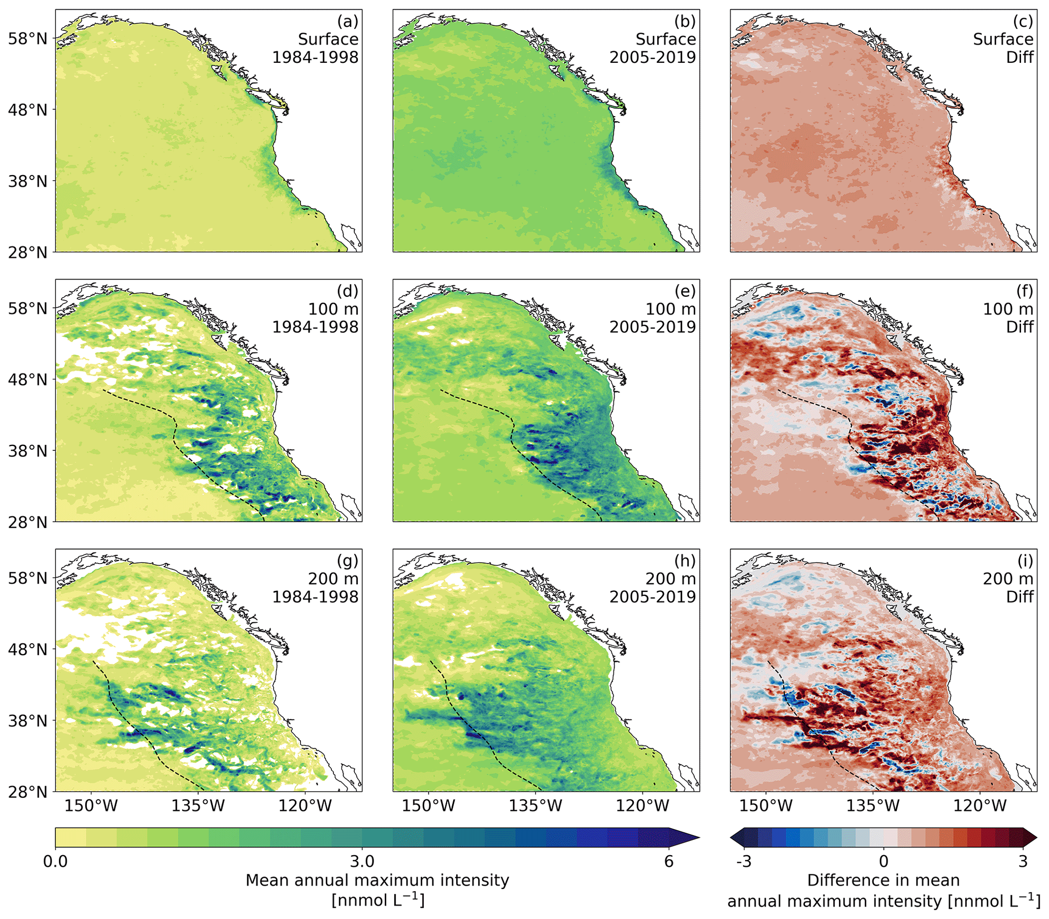
Figure 4Maps of the average annual maximum intensity of [H+] extremes for (a, d, and g) the period 1984–1998, (b, e, and h) 2005–2019, and (c, f, and i) the difference between the two periods. (a–c) Average conditions and difference for the surface layer. (d–f) The same as (a–c) but for a depth of 100 m. (g–i) The same as (a-c) but for a depth of 200 m. For the average, only years with extremes are taken into account. White areas depict areas that did not experience any extremes over the respective decade. The dashed black lines depict the front formed by the maximum extent of the westward-propagating eddies at 100 and 200 m.
By contrasting the above results (Fig. 3; HCast simulation) with those from the CCons simulation, we can attribute the trends in the annual mean duration and annual maximum intensity to the rise in atmospheric CO2. This comparison shows that, as was the case for the volume of OAX, the increases in duration and maximum intensity are almost exclusively driven by the increase in atmospheric CO2 (not shown).
3.3 Heterogeneous distribution of OAX intensities
The highly spatially aggregated data in Fig. 3c and f hide the existence of substantial spatial differences in the distribution of the annual maximum intensities, especially at depth (Fig. 4). While the annual maximum intensities and their changes with time tend to be spatially relatively uniform at the surface, these intensities and changes are spatially very heterogeneous at depth. Particularly striking is the presence of a front at about 1500 km from the west coast of the Americas, separating waters with very high maximum intensities of OAX to the east from waters with relatively low maximum intensities to the west. In fact, some of the highest maximum intensities are found just to the east of this front. As shown by Desmet et al. (2022), this pattern of OAX intensities is the consequence of what they called “large, long, and propagating” (LLP) OAX. These LLP OAX events originate near the coast of the Americas and then propagate for months and years westward. They harbor rather intense extremes as a consequence of encapsulating low pH and low ΩA waters during their formations near the coast by isolating the extreme conditions within them owing to their rotation and by partially enhancing these OAX conditions throughout their lifetime by enhanced export production and remineralization at depth, increasing [H+].
In our model simulations, these LLP OAXs dissipate at this intensity front, causing a very rapid drop-off of the maximum intensity to the west of it. This drop-off is located a few hundred kilometers closer to the shore at 100 m depth compared to the situation at 200 m depth. The presence of this front was the reason for separating the open-ocean region into two subregions, i.e., the ONP and CNP (see Sect. 2.4 and Appendix A, where we used the average position of the front at 100 and 200 m to delineate these two regions). In the open-ocean regions east of this front, i.e., in the ONP, the map reveals a highly patchy distribution of high maximum intensities, reflecting the pathways of the episodic high LLP events. Inside these LLP, the annual intensities can reach values of well above 5 nmol L−1. In contrast, the annual maximum intensities to the west of this front are generally less than 1 nmol L−1. The pattern of the increase in the maximum intensities follows the spatial distribution of average annual maximum intensity seen in both 15 years periods (contrast panels Fig. 4f and i with panels Fig. 4d, e and g, h, respectively, in Fig. 4), with increases in many places of up to 3 nmol L−1. This implies that the lines for the open-ocean regions in Fig. 3f represent an average of two subregions with distinctly different OAX intensities and changes thereof.
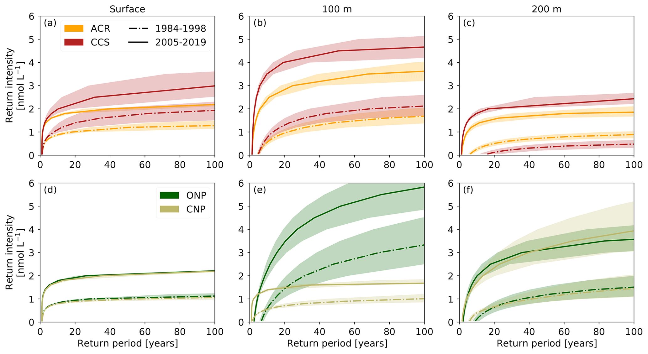
Figure 5Return intensity (in nmol L−1) as a function of the return period (in years) for the HCast scenario at (a) surface, (b) 100 m, and (c) 200 m depth in the (a–c) ACR and CCS and (d–f) ONP and CNP regions for two different time periods, respectively, 1984–1998 (dashed–dotted) and 2005–2019 (solid). The line represents the median and the shading the 40th–60th percentile interval based on the spatial variability within each region.
3.4 Change in return intensity
The rapid increase in intensity of [H+] extremes causes between the first and last 15 years of the hindcast a substantial increase in the [H+] intensity associated with a given return period (Fig. 5). Intensity levels that were rare to unlikely from 1984 to 1998 have become frequent in the last 15 years. For instance, an intensity of 1 nmol L−1 (∼ −0.020 pH unit) was rare at 100 m depth in the CCS (one in 13.3 years event) but occurs every second year in the last 15 years (one in 1.7 years event; Fig. 5b). Similarly, at 100 m depth in the CNP, such an intensity occurs once in a 100 years based on the data of the first 15 years. Then, 20 years later between 2005 and 2019, such an event is estimated to occur every second year (one in 2.2 years event; Fig. 5e). Changes in the return period of high intensities are also large. An intensity of 4 nmol L−1 (∼ −0.087 pH unit) would not occur in 100 years at 100 m depth based on the data of the first 15 years while it represents an event that happens every 1 in 19.2 (27.1) years in the CCS (ONP) in the last 15 years (Fig. 5b and e).
As with the other metrics, the return intensities and the magnitude of their change vary spatially and with depth. At the surface, the changes in the return intensity tend to be smaller than in the subsurface and similar between regions to what they are for the intensity itself (Figs. 4c and 5a, d). The largest changes in return intensity occur at 100 m depth, in particular in inshore areas and in the ONP region where the 1-in-10-years return intensity increases by 2.07 nmol L−1 (∼ −0.048 pH unit) on average (from 0.63 to 2.71 nmol L−1; Fig. 5b and e). Finally, some regions exhibit substantial spatial variability in the return periods associated with given return intensity (Fig. 5). The largest spatial variability is found at 100 m depth in the ONP region, matching the strong variance of OAX maximum intensity in this region (Figs. 4d, e and 5e).
Overall, the rate of change in OAXs and their characteristics in response to the increase in atmospheric CO2 varies in space and depth (Figs. 2–5). While the surface response is rather linear in time and homogeneous in space, the subsurface response is more variable and depends on the marine environment being an inshore or offshore regime or an intermediate offshore regime with substantial coastal imprint from mesoscale eddies.
3.5 Rapid versus delayed emergence of near permanent OAX
While the volume of OAX already revealed some substantial nonlinear response to the rise in atmospheric CO2 with abrupt onsets and rapid expansions (Fig. 2), the last metric of interest, i.e., the number of extreme days per year, shows the most striking pattern of abruptness (Fig. 6). The increase in yearly extreme days between the first and last 15 years of the hindcast shows sharp spatial transitions at all depths but distributed heterogeneously in space with large differences in the magnitude of the increase. The increases in the number of extremes days reach up to more than 200 d, leading to almost year-round OAXs towards the end of the hindcast in some locations (Fig. 6f).
The strongest step increases in the yearly number of extreme days occur in the subsurface of the CNP (Fig. 6d–f). In only 2 years (between 2004 and 2006), the yearly number of extreme days at 200 m at point PCNP jumps from ∼ 30 to more than 300 d (Fig. 6f). Similarly, at 100 m depth, the yearly number of extreme days jumps from ∼ 30 to 150 d in 1 year (1994–1995) and to more than 300 d 6 years later (2001). These local step responses are also seen in the OAX volume fraction of the 50–100 m depth layer of the CNP (Fig. 2k), although the step response tends to be masked by the aggregation that occurs when the volume fraction is computed. In contrast, no such step response occurs during our analysis period in the subsurface central CCS and ∼ 1000 km offshore (PCCS and PONP), where only a small increase in yearly extreme days is seen (Fig. 6). OAXs remain episodic even towards the end of the hindcast under elevated atmospheric CO2 levels (Fig. 6d and e). At the surface, a large increase in yearly extreme days is found in most areas except the coastal central CCS (Fig. 6a). Overall, the area experiencing large increases shrinks with depth. In the subsurface, the sharp spatial transition in the response coincides with the front in annual maximum intensity and its change (Fig. 4d–i) described in Sect. 3.1, as well as with the westward extent of eddy-driven OAXs, i.e., the eddy propagation front (dashed black lines in Figs. 4 and 6).
The spatial pattern of the large versus small increase in yearly extreme days is well reflected in the spatial distribution of the ToE (Fig. 7). The area experiencing near-permanent OAX before the end of the hindcast (ToE ≤ 41 years) decreases with depth. At the surface, 88 % of the northeastern Pacific experiences near-permanent OAX in 2019 (Fig. 7a). Only the CCS and ACR have a stronger surface [H+] variability than surface [H+] trend under increasing atmospheric CO2 within the time frame of the hindcast. In the subsurface, however, only 40 % and 15 % of the northeastern Pacific at 100 and 200 m depth, respectively, experiences near permanent OAX in 2019 (Fig. 7b and c). At both 100 and 200 m depth, ToE less than ∼ 40 years is confined to the offshore regions that do not have an imprint from coastal variability, i.e., in the CNP west of the eddy front. At PCNP, the ToE is as short as 18 years at 100 m depth, matching the early step response in yearly extreme days seen at that location (Fig. 6f).
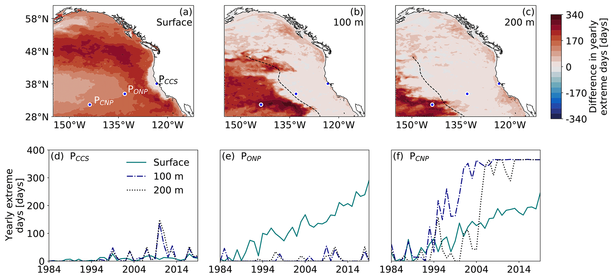
Figure 6Spatiotemporal progression of the yearly [H+] extreme days in the northeastern Pacific. (a) Map of the difference in yearly [H+] extreme days between 2005–2019 and 1984–1998 in the HCast simulation at the surface. (b) The same as (a) but for 100 m depth. (c) The same as (a) but for 200 m depth. The three blue disks with white contours in each map denote the locations for the time series in panels (d–f), reflecting a location in the nearshore CCS (d), a location in the ONP region (e), and a location in the CNP region (f). The dashed black lines in (b, c) denote the location of the westward eddy propagation front.
4.1 OAX increase in response to the rise in atmospheric CO2
The increasing rates of the yearly number of extreme days and duration and intensity of OAX with respect to increasing atmospheric pCO2 found in our study are in the same order of magnitude as the ones estimated in previous OAX studies in the global ocean over the historical period 1861–2005 (Burger et al., 2020; Gruber et al., 2021). The similarity in the rates of increase despite the different time frames of the two compared periods (145 versus 36 years) underlines the key role of atmospheric pCO2 in OAX increase over time. Despite different models used and associated distinct resolutions, the surface increase rates in number of OAX days are similar between our study (3.7 d µatm−1) and the study by Burger et al. (2020) (cf. Fig. 4a in their study). In the subsurface, however, the increase rate in number of extreme days and OAX duration largely differs between the two studies. The increase in number of extreme days at 200 m depth is almost 3 times slower in our study than in Burger et al. (2020) (cf. Fig. A1e of their study), and a similar difference is found for OAXs duration (cf. Fig. A1c and d in Burger et al., 2020). In subsurface waters, where mesoscale processes, such as eddies, largely contribute to broaden the distribution of [H+] (Appendix Fig. B6e and f), differences in OAX increase rate are more dependent on the model resolution than at the surface. In our high-resolution eddy-resolving study, broader distributions lead to thresholds more distinct from the mean than in the coarser-resolution models that do not resolve mesoscale processes. This likely led to the slower but more realistic subsurface increase in number of OAX days and OAX duration in our study with respect to increasing atmospheric pCO2.
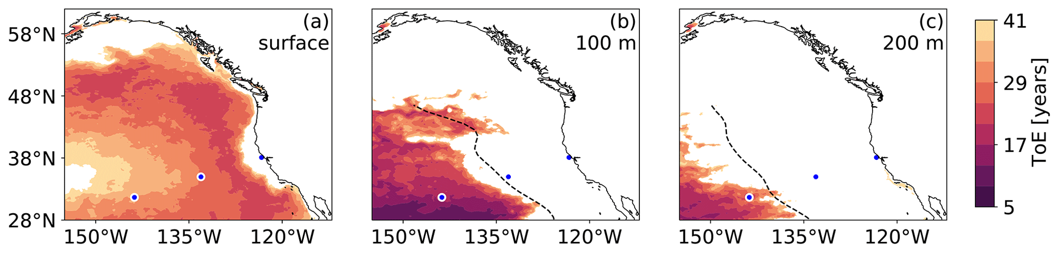
Figure 7Maps of the time of emergence (ToE) of the yearly mean [H+] (long-term trend in [H+]) above the local [H+] threshold at (a) the surface, (b) 100 m depth, and (c) 200 m depth in the HCast simulation. White areas denote regions where the long-term trend does not exceed the threshold at the end of 2019 (i.e., ToE > 41 years). The three blue disks with white contours in each map denote the locations where the time series in Figs. 1 and 6 were extracted. The dashed black lines denote the westward eddy propagation fronts.
Emphasizing the rapidity of the changes in OAX is the drastic reduction in the return period of high intensities between the 1984–1998 and 2005–2019 periods. In less than 40 years, extremely rare (≫ 100 years) high intensities become a one in less than 30 years event. Similarly, a strong reduction in the return periods of intense marine heat waves is projected under global warming (Laufkötter et al., 2020). The rapidity of the change is further corroborated by the near permanency of OAXs that is reached in a large fraction of the upper 250 m of the northeastern Pacific within the time frame of our hindcast. The near permanency of extreme conditions has also been projected to occur between 2030 and 2050 for aragonite undersaturation events (absolute threshold) at the seafloor of the 10 km coastal CCS (Hauri et al., 2013a). From a mean duration of 16 d in 2010, those events are projected to reach near permanency in less than 40 years (Hauri et al., 2013a). In our study, however, OAXs, defined based on a relative threshold, do not reach near permanency in the CCS given the strong natural variability of the region. This highlights the very different perspectives of using absolute versus relative thresholds to define extreme events.
When using a relative threshold and a fixed baseline to define OAX, the ratio of the long-term trend to local variability is key in determining the increase in OAX. Thus temporal changes in the variability can have a substantial influence on the evolution of the OAX. Such an increase in variability is actually expected as a consequence of ocean acidification (see also Burger et al., 2020), driven by the increase in the hydrogen ion concentration and a higher sensitivity to change. The variability can also change as a consequence of changes in weather and climate. In our simulations, the variability of [H+] increases in all surface regions and in the subsurface of the CCS, ONP, and CNP regions (Appendix Fig. B5). However, these increases in variability tend to contribute comparatively little to the overall increases in the OAX. We can estimate this contribution most easily in the regions where the [H+] distributions are Gaussian (e.g., at 100 m depth of PCCS). There, the increase in variability increases the number of OAX days by a factor of 1.3, which is an order of magnitude smaller than the impact of the change in the mean state, as this leads to a 14-fold increase. Similarly, the maximum OAX intensity would increase by only 2 % from the change in variability versus the intensity increasing by 82 % from the change in mean state.
4.2 Spatial heterogeneity in OAX increase
Although rapid, changes in OAX are spatially heterogeneous in the northeastern Pacific. While OA trends are of similar magnitude between the studied regions and depths, differences in types and magnitudes of the marine environment's natural variability lead to varying increases in OAX (Fig. 8). The relatively slow and progressive increase in OAX in the nearshore central CCS can be explained by the strong natural variability of the region. The amplitude of surface [H+] variability is about 6 times larger than the magnitude of the OA trends from 1984 to 2019 (Appendix Fig. B6a). The same variability versus trend pattern and subsequent OAX response holds for the subsurface. While it is beyond the scope of this work to assess the mechanisms driving the strong year-to-year variability in OAXs in the coastal regions (Sect. 3.1), this variability largely correlates with the El Niño–Southern Oscillation, particularly impacting OAX in coastal regions of the northeastern Pacific, as shown in Desmet (2022). In contrast to the nearshore CCS, ∼ 1000 km further offshore and in the CNP region, the amplitude of surface [H+] variability is closer to the magnitude of OA trends (ratio of 1.14 at PONP and 1.17 at PCNP), leading to the strong and rapid increase in OAX. The more similar amplitudes of variability and trends in these regions is due to a 5 times smaller surface variability compared to the nearshore CCS (Appendix Fig. B6a–c). Consistent with the even larger and faster increase in yearly OAX days found in the subsurface CNP is the even lower variability over trend ratios in the subsurface CNP (Fig. B6f and i). In the subsurface waters off central CCS (ONP region), however, we found a much weaker increase in OAX. While the amplitude of the variability within the inter-decile range is small and comparable to the one of the subsurface CNP, high [H+] signals are episodically reached (Appendix Fig. B6e). These short and episodic high [H+] signals have an amplitude above the upper bound of the inter-decile range 7.9 (3) times larger than the amplitude of the inter-decile range itself at 100 m (200 m) depth, leading to a highly right skewed natural variability distribution (Appendix Fig. B6e). This skewness delays the emergence of OA trend over the threshold (e.g., Fig. 8c), which explains the weaker increase in OAX (Figs. 2h, i and 6e).
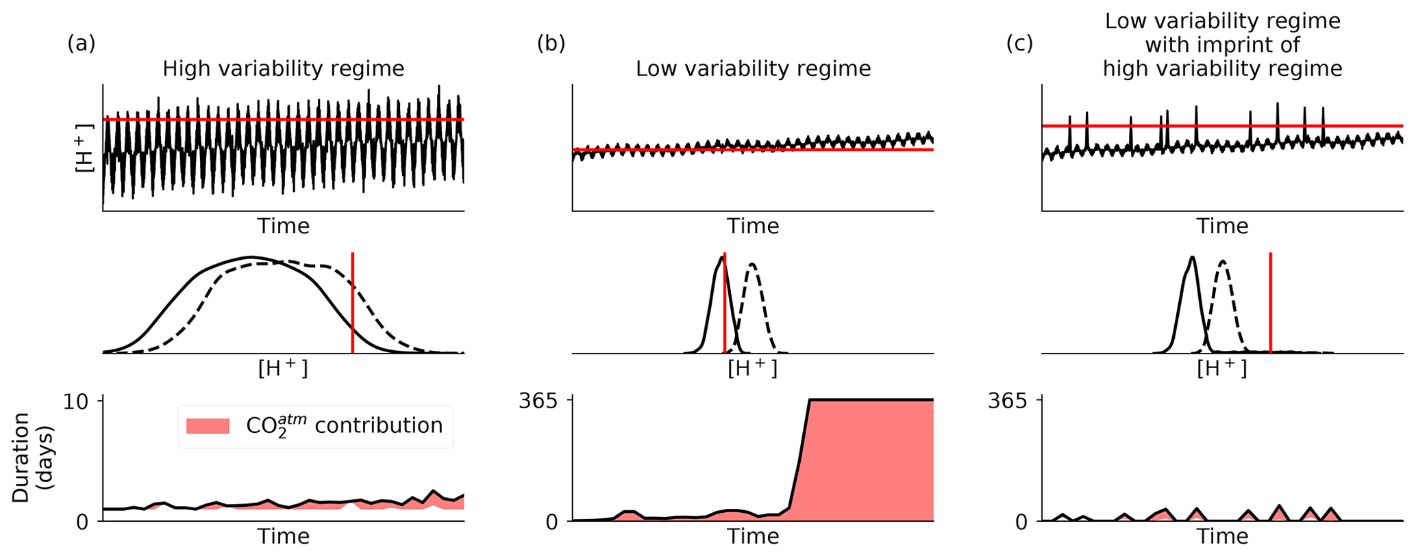
Figure 8Schematic of three different [H+] variability regimes (a–c) that lead to three different responses with regard to OAX under the same long-term increase in [H+] from the rise in atmospheric CO2. The top row shows illustrative 36-year daily time series and their respective 99th percentile threshold computed on the linearly detrended time series. The middle row shows associated probability density functions of the first (solid lines) and last (dashed lines) decades with the same threshold as above (red). The bottom row shows associated annual mean event duration (in days). The red-filled area depicts the difference in annual mean event duration between the time series with and without the long-term trend, i.e., illustrating the contribution of atmospheric CO2 rise to the temporal change in annual mean event duration. Note the different scale in the left plot. A low-frequency modulation, representing decadal climate variability, is included in all three signals.
In addition to the spatial heterogeneity in the magnitude of OAX increase, the abruptness of the change also varies spatially, with the strongest step increase in OAX occurring in the subsurface CNP (Sect. 3.5, Fig. 6f). In light of the relative threshold used in this study, such nonlinearities imply that marine organisms may suddenly experience much more often conditions at the edge or outside the local environmental conditions to which they tend to be adapted to, with potential deleterious effects on their fitness (Vargas et al., 2017, 2022; Kroeker et al., 2020; Rivest et al., 2017; Cornwall et al., 2020). While the large increase in OAX in low variability regions, such as the subsurface CNP, results from the rapid exceedance of the variability by OA trends (e.g., Fig. 8b), the nonlinearities (step increases) found in those same regions (Sect. 3.5, Fig. 6f) may result from the concurrent effect of OA trends and synergistic low frequency (decadal to multi-decadal) climate variability, as illustrated in Fig. 8b. Indeed, the occurrence and intensity of OAXs in the CCons simulation correlate with decadal climatic modes such as the North Pacific Gyre Oscillation (Desmet, 2022). Therefore, low-frequency climate variability is likely to modulate, i.e., mitigate or amplify in turn, the imprint of OA trends on OAX. In low natural variability regions, the interaction between OA trends and climate variability may be the cause of a sudden widespread crossing of the threshold, when both act in the same direction at the time when the mean state approaches the threshold (Fig. 8b). The timing of the step increases in OAXs in our study may therefore relate to the atmospheric forcing and would probably vary if we were to run a coupled model, which would have its own decadal and year-to-year variability.
Differences in the natural variability of the ocean carbonate chemistry are also reflected in the regionally different ToEs. We find shorter ToE in the surface subtropical oligotrophic gyre (∼ 16 years), a longer ToE in the surface offshore subarctic region (∼ 25 years), and an even longer ToE in surface coastal areas, both along the Alaskan and the US west coasts (∼ 30–32 years to no emergence yet in 2019). The ordering of these results is consistent with results from observations with the station ALOHA in the subtropical oligotrophic gyre having the shortest ToE in the northeastern Pacific (9 years), closely followed by station Papa in the offshore subarctic (10 years), and then by coastal sites (12–23 years) (Sutton et al., 2019). The ToEs found in our study are about 1.5 to 2.5 times larger than those found in Sutton et al. (2019). This is also true when comparing to pCO2 and pH ToE found in Keller et al. (2014). However, these differences are consistent with the differences in definitions, with our detection threshold being more restrictive than in Keller et al. (2014), and with the absence of seasonal variability in the background monthly variability used by Sutton et al. (2019), as well as the absence of intra-annual variability in Keller et al. (2014).
As pointed out with regard to the emergence of OA trends in Sutton et al. (2019), our study underlines the importance of the natural variability of the ocean carbonate chemistry with respect to the response of OAX to anthropogenic changes. Our results based on a high spatiotemporal resolution model show that the emergence of near-permanent OAXs is substantially delayed in coastal regions, as well as quite far offshore at depth in regions that see the mesoscale imprint of nearshore conditions (cf. white areas in Fig. 7).
4.3 Delayed emergence of near-permanent subsurface OAX by mesoscale cyclonic eddies
In the subsurface of the ONP region, the shape of OAX (Fig. 1a) and the spatial pattern of annual maximum intensity (Fig. 4d–i) relate to mesoscale eddy tracks (Sect. 3.3). The distinctive pattern of subsurface maximum intensity does not appear in the analyses of Burger et al. (2020) (cf. Fig. 7d in their paper). We also do not expect it to appear since the resolution of their model is much coarser (horizontal resolution of ∼ 80 km), preventing it from resolving the mesoscale processes that we identify as shaping these spatial heterogeneities in subsurface OAX maximum intensity. This is consistent with previous findings based on a Lagrangian perspective that found mesoscale cyclonic eddies to be important drivers of OAX in the subsurface of the northeastern Pacific (Desmet et al., 2022). Moreover, the sharp spatial boundaries between short (∼ 22 years on average) and long (∼ 32 years on average) ToE in the subsurface, and the corresponding boundaries between large (+248 d on average) and small (+36 d on average) increases in yearly extreme days and annual mean event duration from 1984 to 2019, correspond well to the westward extent of cyclonic eddy-driven OAXs in the northeastern Pacific (Appendix A, Figs. 6b, c and 7b, c). This result suggests that mesoscale cyclonic eddies substantially enhance the amplitude of the background variability at depth in the open ocean, and, as a result, lead to large threshold values relative to the mean of local [H+] distributions (Appendix Figs. B6e and A1). This eddy-induced variability substantially delays the ToE of OAX and reduces the increase in yearly extreme days and event duration in comparison to open-ocean regions experiencing weak mesoscale activity. This is consistent with our subsurface rates of increase in the number of extreme days and OAX duration being lower than in previous global ocean studies that are based on global Earth system models that do not fully resolve mesoscale variability (Sect. 4.1).
The cyclonic eddy-driven OAX westward propagation front defined in our study resonates well with previous findings on the offshore imprint of nearshore waters from cyclonic eddies (Zhao et al., 2021; Chabert et al., 2021; Amos et al., 2019; Chenillat et al., 2016; Nagai et al., 2015). They show that cyclonic eddies maintain locally elevated nutrient concentrations, productivity, and organic matter in the offshore regions more than 1000 km away from the CCS coast. Subsurface coherent eddies originating from the eastern boundary poleward undercurrents (“Puddies”) have been shown to contribute to low-oxygen extreme events and to reach thousands of kilometers offshore in the subsurface (Frenger et al., 2018). These Puddies have their core between 100 and 700 m depth, matching the absence of eddy front signal in surface OAX and its presence at 100 and 200 m depth. Furthermore, the depth dependency of our eddy front is consistent with Puddies sliding along isopycnals and subducting from the nearshore formation regions into the gyre interiors (Frenger et al., 2018). Finally, the presence of such an eddy front is consistent with mesoscale eddies decaying after a certain distance from the coast (Frenger et al., 2018; Chenillat et al., 2016). However, the exact location of this front may be altered by the non-uniform spatial resolution of the telescopic grid, potentially accelerating the decay of mesoscale eddies in our model as the resolution coarsens.
4.4 Limitations and caveats
As the science of ocean acidity extreme events is only in its early stage, there is no consensus yet on the definition of OAX. In this study we use a common Eulerian event-based framework on a single carbonate variable criterion. Several other definitions have been used in previous works, such as in Desmet et al. (2022), where a Lagrangian approach in three dimensions on a dual variable criterion (pH-ΩA) was taken to define extremes. We expect the Lagrangian pH-ΩA extreme events to have similar temporal responses to the increase in atmospheric pCO2 to the ones found in this study. Yet, a few differences might ensue from the dual variable criterion and the Lagrangian framework. The former may lead to a different temporal response of OAX in the surface of the ONP and CNP regions, with an abrupt increase in contrast with the linear increase found in our study. Indeed, in these surface offshore areas, where pH and ΩA are seasonally out of phase, pH-ΩA extremes will likely occur only once both variables start to be below the lower bound of their variability in the reference period regardless of the season (Xue et al., 2021; Kwiatkowski and Orr, 2018; Desmet et al., 2022). As regards the Lagrangian framework, since we find near-permanent extreme conditions in a large fraction of the upper 250 m of the northeastern Pacific, one can expect a single large Lagrangian OAX to form towards the end of the analysis period, with a mean volume close to the entire volume of the upper 250 m of the northeastern Pacific. This may limit the relevance of the Lagrangian definition of OAX when using fixed baselines on reference periods with past atmospheric pCO2 levels such as preindustrial levels or even levels of a few decades earlier, as in this study, due to the rapid OA trend.
The use of relative thresholds on fixed baselines to define OAX requires the model to accurately capture OA trends since the ratio of the long-term trend to local variability is key in determining the increase in OAX in that case. Giving us confidence in our results are the well-captured pH and ΩA surface trends over the last 4 decades in our model. Yet, in the subsurface, simulated dissolved inorganic carbon trends tend to be higher than suggested by observations, even though substantial uncertainties associated with the observation-derived trends exist (Franco et al., 2021). If this model subsurface bias holds up to further scrutiny and for other carbonate variables such as [H+], it would imply a slower increase in subsurface OAX than simulated. Yet, our conclusions about the large spatial heterogeneity in the progression of OAX and the abruptness of the onset of the OAX in the far-offshore regions would remain unchanged. An alternative to fixed baselines is the use of shifting baseline periods that accounts for changes in the mean state of the marine carbonate system variable of interest over the period for which extremes are analyzed (Burger et al., 2020). In that case, the threshold varies in time, following OA trends. Changes in OAX defined on shifting baselines are therefore not well captured by the ToE concept. What drives their change is instead a modification of the short-term variability, i.e., in the nature of the underlying distribution, of the marine carbonate system variable of interest. This leads to larger disparities in the changes in OAX defined with respect to different carbonate variables than when using fixed baselines (Burger et al., 2020). At the global scale, [H+] extremes defined on shifting baselines exhibit large increases in their volume, duration, and intensity in the upper 200 m depth, whereas ΩA extremes follow a decreasing pathway. In our study, a change from fixed to shifting baseline would result in a slower progression of [H+] extremes over the course of the analysis period. However, spatially heterogeneous increases in OAX are still expected to be found given the expected different changes in the short-term variability of the carbonate variables between regions and depths stemming from the many processes in play – e.g., long-term changes in upwelling, eddy activity, buffer factor, or temperature – and their varying relationship with the different carbonate variables. The ecological relevance of using a fixed versus shifting baseline to define OAX depends on the level of adaptive capacity of marine ecosystems to long-term changes in OA and on the timescales of this potential adaptation (Oliver, 2019; Oliver et al., 2021; Gruber et al., 2021). Yet, the level of adaptive capacity of marine ecosystems to long-term changes in OA is still unclear (Mekkes et al., 2021; Bednaršek et al., 2016, 2017, 2021; Manno et al., 2017). The use of a fixed baseline, as chosen in our study, allows for capturing changes in OAX ensued from both long-term anthropogenic and short-term variability changes that add up and may together lead to episodic crossings of biological thresholds (Doney et al., 2020; Bednaršek et al., 2017).
In addition to the detection of extremes with regard to [H+], we quantify the proportion of [H+] extremes that are undersaturated with regard to aragonite, since ΩA = 1 is a well-known threshold for OA impacts on shelled marine organisms such as pteropods (Bednaršek et al., 2014). However, different thresholds may be relevant for different organisms, life stages, and durations of exposure (Bednaršek et al., 2019; Fabry et al., 2008). For instance, supersaturated waters with ΩA below 1.5 have also been found to cause mild and severe dissolution of pteropods shell (Bednaršek et al., 2019). When quantifying the proportion of OAXs that are in waters with an ΩA below 1.5, cross-shore and cross-depth patterns similar to those found for a threshold of ΩA = 1 (Sect. 3.1) were found (Appendix Table B1).
As for the undersaturation criterion, most of the surface OAXs and most of the CNP OAXs have ΩA above 1.5. However, in the CNP 50–100 m depth layers, 1 % of OAX volume have ΩA levels below 1.5 while none is undersaturated yet (Appendix Table B1 and Table 2). The analysis for ΩA < 1.5 also reveals that most of the newly undersaturated OAXs found in the 50–100 m depth layer of ACR and CCS occur in waters that were only weakly supersaturated (ΩA < 1.5) in the CCons simulation (Table 2 and Appendix Table B1). This result is consistent with previous findings on low aragonite saturation state events (i.e., extremes defined based on absolute thresholds) that show a projected rapid increase in the duration of undersaturation events at the seafloor of the nearshore CCS, already weakly supersaturated with regard to aragonite in the preindustrial period (ΩA permanently under 1.4; Hauri et al., 2013a). It suggests that organisms hit by newly undersaturated OAXs may already be, in most of the cases, adapted to near-corrosive conditions.
Our study highlights the rapidity of the increase in ocean acidity extremes, in agreement with previous regional and global scale studies on past and projected changes (Hauri et al., 2013a; Burger et al., 2020; Gruber et al., 2021). What was defined as rare high-acidity events in the past, i.e., relative to atmospheric CO2 concentrations of 1979 in our study, has already become a near-permanent state over large areas in the upper 250 m of the northeastern Pacific, albeit with important regional variations. Knowledge of the impacts of present-day extremes on organisms and ecosystems may therefore offer a glimpse of the future health of the ocean in the near future at the surface and offshore and in the more distant future in coastal subsurface regions given the spatial heterogeneity in increasing rates of acidity extremes.
The increase in ocean acidity extremes from 1984 to 2019 in the northeastern Pacific is mostly driven by the rise in anthropogenic atmospheric CO2. Present-day trends in ocean acidity extremes will therefore continue as atmospheric CO2 continues to rise or even accelerate as the buffer capacity of the seawater declines, especially in regions with already low buffering capacity, such as the Alaskan coast and the nearshore California Current System (Cai et al., 2020; Feely et al., 2018; Jiang et al., 2019). This is worrisome in the context of the constantly growing anthropogenic CO2 emissions (Friedlingstein et al., 2019), especially as a large fraction of these high-acidity extremes also cross well-known biological thresholds of aragonite saturation state. Furthermore, nonlinearities in the increase in extremes defined on relative thresholds, such as those found in our study, imply that organisms may suddenly experience conditions at the edge or outside the variability range of their local environment much more often. This may lead to deleterious impacts on marine organisms since they tend to be adapted to their local environment and its variability (Vargas et al., 2017; Kroeker et al., 2020; Rivest et al., 2017; Cornwall et al., 2020).
While the strong ocean acidification trend overtakes the natural variability over large areas in the upper 250 m of the northeastern Pacific, interannual variability still drives the occurrence of acidity extremes in subsurface coastal regions substantially. In the California Current System, the El Niño–Southern Oscillation is likely to be a strong modulator of ocean acidity extremes on interannual timescales, since it modulates the biogeochemistry of the region (Turi et al., 2018; Frischknecht et al., 2015). Studies that assess the response of acidity extreme events to climatic modes are needed and could further be used to forecast the occurrence and intensity of acidity extremes in coastal regions of the northeastern Pacific. Besides interannual variability, our study uncovers the key role of mesoscale activity in slowing down the increase in acidity extremes in the subsurface of intermediate offshore regions compared to previously found increases in global scale studies (e.g., Burger et al., 2020). This implies that ocean acidity extremes in those regions may increase less rapidly than projected by Earth system models (Burger et al., 2020), since these models often miss the strong variability induced by mesoscale activity.
We identify the westward eddy propagation front at 100 and 200 m depth between 28 and 47∘ N as the farthest distance to the coast where at least one eddy-driven OAX, i.e., one “large, long, and propagating” (LLP) OAX (Desmet et al., 2022), passes every 5 years. The rationale for this choice is the following. In offshore regions with a small variability range, eddies need to be present more than 1 % of the time to significantly affect the threshold defined as the 99th of all aggregated daily value at a given location, i.e., more than 132 d in our case from 1984 through 2019 (Fig. A1). Eddy-driven OAXs, as found in previous work by Desmet et al. (2022), have an average local duration of 18 d both at 100 and 200 m depth, meaning that they stay on average 18 d at a given location. Thus, a location must see on average seven of these eddy-driven events over the entire period for its threshold to be substantially moved away from the mean variability range (Fig. A1), i.e., at least one eddy-driven OAX every 5 years. For each LLP event of Desmet et al. (2022), we first compute its maximum distance to the coast and the associated latitude. We then bin these events based on the latitude at which they are the farthest away from the coast into 1∘ latitudinal bands between 28 and 47∘ N. Within each latitudinal bin we select the seventh maximum distance to the coast to make sure that at least seven eddy-driven OAXs reach this distance from the coast. In a last step we apply a Gaussian smoothing (σ = 2∘ N) to the eddy front.
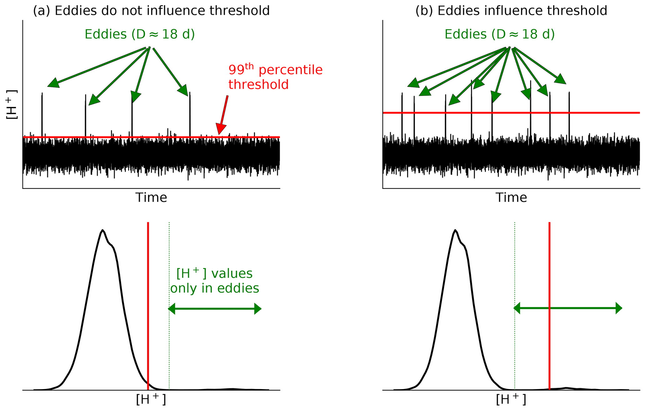
Figure A1Schematic of [H+] daily variability in (a) a region where the threshold is not influenced by passing mesoscale eddies and (b) a region where the threshold is shifted away from the normal distribution due to a high number of passing eddies. In (a), the high [H+] signals carried by eddies account for less than 1 % of the total days (≈ 4 × 18 d ≈ 72 d, while 1 % of the days from 1984 to 2019 would be 132 d) and therefore does not influence the threshold that remains below the high [H+] values carried by eddies. In (b), the high [H+] signal of eddies accounts for more than 1 % of the total days (≈ 8 × 18 d ≈ 144 d) and therefore raises the threshold to a value within the range of high [H+] values carried by eddies.
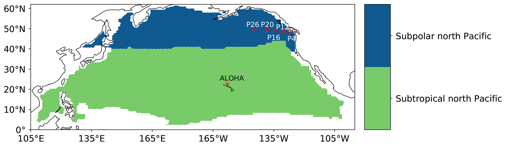
Figure B1Biomes and stations used to evaluate ROMS-BEC surface pH and ΩA long-term trends against observations from Lauvset et al. (2015); Franco et al. (2021); Bates et al. (2014) in Table 1.
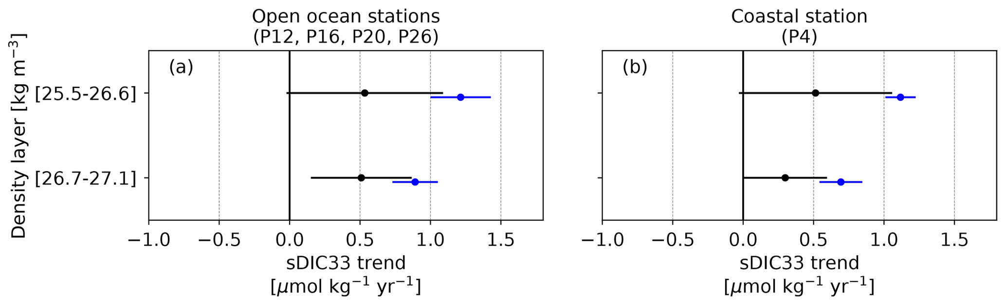
Figure B2Trends in dissolved inorganic carbon normalized to a salinity value of 33 psu (sDIC33) in the subsurface of line P (in ). (blue) Simulated ROMS-BEC trends and (black) observed trends from Fig. 6 in Franco et al. (2021). The trends have been averaged within two density layers, namely mixed-layer and pycnocline waters (25.5–26.6 kg m−3) and intermediate waters (26.7–27.1 kg m−3), as well as across the four open ocean stations (P12, P16, P20, P26) in panel (a). Black error bars denote the average of the 2 standard deviation credible interval (95 % CrI) of individual data points from Fig. 6 in Franco et al. (2021), while blue error bars denote the spatial standard deviation across stations and density levels from ROMS-BEC-simulated trends.
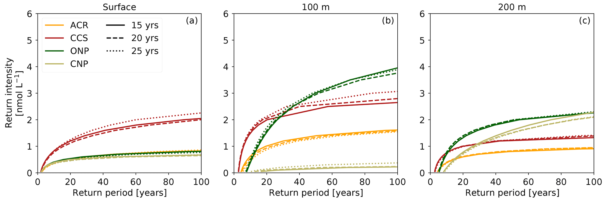
Figure B3Return intensity (in nmol L−1) as a function of the return period (in years) at the (a) surface, (b) 100 m, and (c) 200 m depth in the ACR, CCS, ONP, and CNP regions and for time periods of 15 years (solid; 2005–2019), 20 years (dashed; 2000–2019), and 25 years (dotted; 1995–2019) in the CCons simulation. The line represents the median based on the spatial variability within each region.
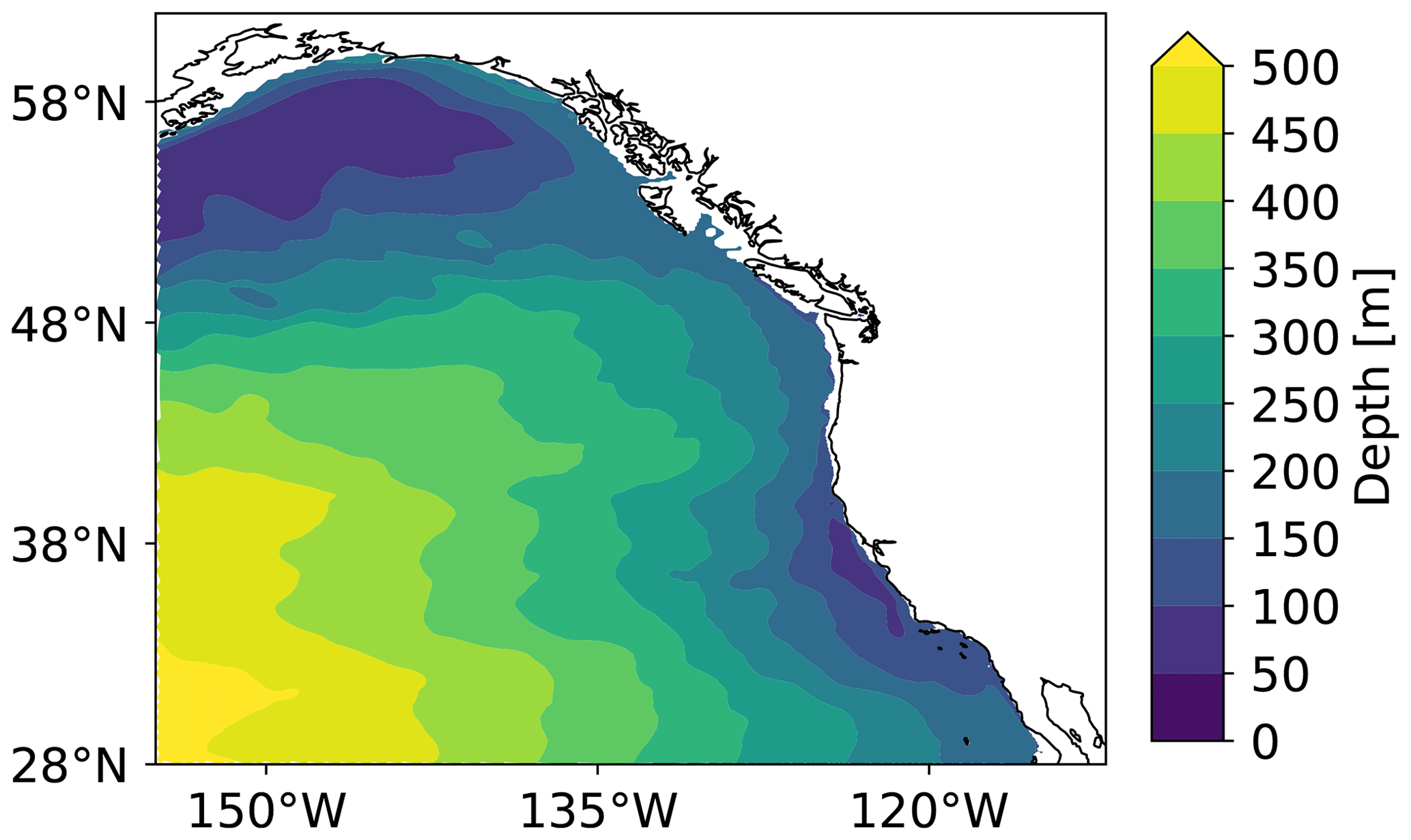
Figure B4ROMS-BEC-simulated climatological (1984–2019) annual mean depths of the ΩA saturation horizon (ΩA=1) in the CCons simulation.
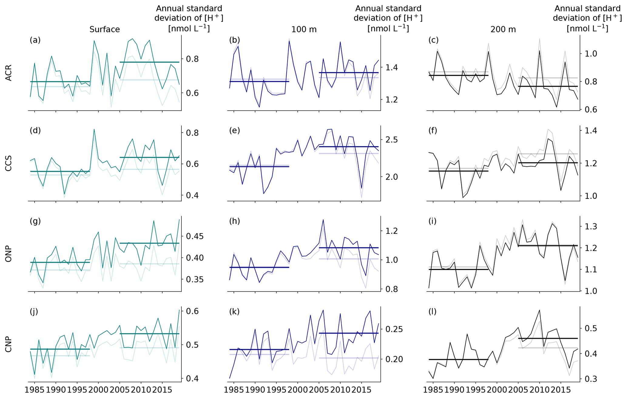
Figure B5Changes in annual standard deviation of [H+] in the HCast (dark) and CCons (light) simulations for the four regions (rows) and three depth layers (columns). The horizontal lines depict the average standard deviation during the 15 first and last years of the analysis period for each simulation.
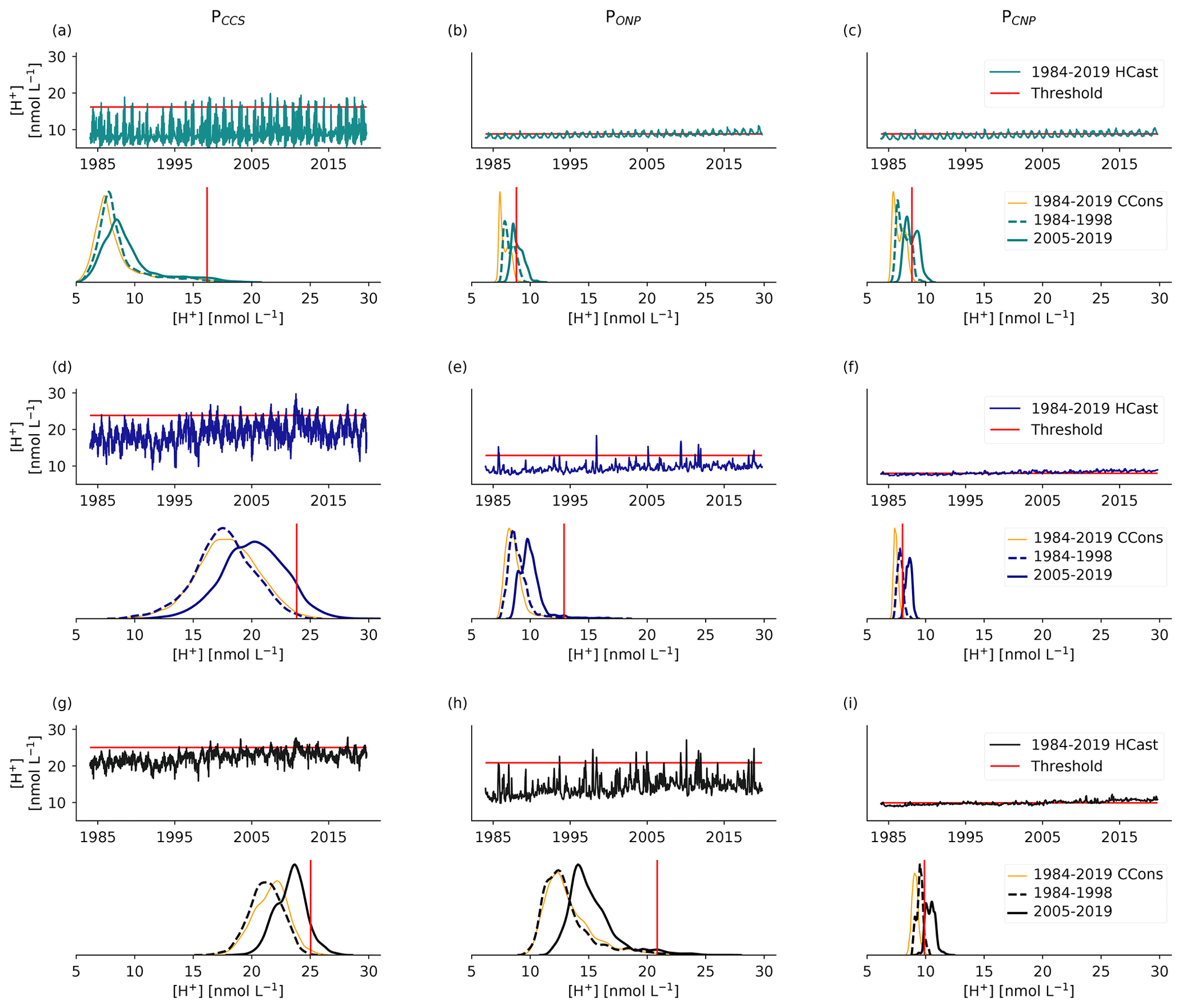
Figure B6Time series and probability density functions (PDF) of [H+] (nmol L−1) at the three locations plotted in Fig. 6 for (a–c) surface, (d–f) 100 m depth, and (g–i) 200 m depth in the HCast simulation. The respective [H+] thresholds are plotted in red. In the PDF plots, the PDF over the entire period (1984–2019) in the CCons simulation is plotted in orange and the PDFs of the 1984–1998 and 2005–2019 periods of the HCast simulation are plotted in cyan, blue, and black depending on the depth with a dashed and solid line, respectively. The periods correspond to the periods used for the difference maps in Figs. 4 and 6.
Table B1Fraction (in %) of the OAX volume that is characterized by ΩA < 1.5 conditions with regard to aragonite averaged over 1984–2019 for the four different regions of the northeastern Pacific shown in Fig. 1a and for three different depth layers. Numbers in the “ΩA newly < 1.5” column give the fraction of the OAX volume that is new in ΩA < 1.5 conditions with regard to aragonite. This is computed by identifying the fraction of the OAX volume that is in ΩA < 1.5 conditions in the HCast simulation but in ΩA ≥ 1.5 conditions in the CCons simulation where atmospheric CO2 was kept at its 1979 value.
The processed data are available online at the ETH library archive (https://www.research-collection.ethz.ch/handle/20.500.11850/604737, last access: 26 October 2023). Model output data may be obtained upon request from the corresponding author (flora.desmet@usys.ethz.ch).
The conceptualization of this research was done by all co-authors. FD performed the simulations and conducted the formal analysis. FD prepared the manuscript with contributions from all co-authors.
The contact author has declared that none of the authors has any competing interests.
Publisher's note: Copernicus Publications remains neutral with regard to jurisdictional claims made in the text, published maps, institutional affiliations, or any other geographical representation in this paper. While Copernicus Publications makes every effort to include appropriate place names, the final responsibility lies with the authors.
The simulations were performed at the HPC cluster of ETH Zürich, Euler, which is located in the Swiss Supercomputing Center (CSCS) in Lugano and operated by ETH ITS Scientific IT Services in Zurich. All further analyses and all figures were created using the software package Python. We thank Meike Vogt for her valuable feedback on an earlier version of the manuscript. The authors also thank the two reviewers for their thoughtful and constructive reviews that helped to improve the article.
This research was supported by the Swiss National Science Foundation under grant agreement no. 175787 (Project X-EBUS), by the Swiss Federal Institute of Technology Zürich (ETH Zürich), and by the European Union's Horizon 2020 research and Innovation Programme under grant agreement no. 820989 (project COMFORT).
This paper was edited by Olivier Sulpis and reviewed by two anonymous referees.
Amos, C. M., Castelao, R. M., and Medeiros, P. M.: Offshore transport of particulate organic carbon in the California Current System by mesoscale eddies, Nat. Commun., 10, 4940, https://doi.org/10.1038/s41467-019-12783-5, 2019. a, b, c, d
Bates, N. R., Astor, Y. M., Church, M. J., Currie, K., Dore, J. E., González-Dávila, M., Lorenzoni, L., Muller-Karger, F., Olafsson, J., and Santana-Casiano, J. M.: A time-series view of changing surface ocean chemistry due to ocean uptake of anthropogenic CO2 and ocean acidification, Oceanography, 27, 126–141, https://doi.org/10.5670/oceanog.2014.16, 2014. a, b, c
Bednaršek, N., Feely, R. A., Reum, J. C. P., Peterson, B., Menkel, J., Alin, S. R., and Hales, B.: Limacina helicina shell dissolution as an indicator of declining habitat suitability owing to ocean acidification in the California Current Ecosystem, P. Roy. Soc. B-Biol. Sci., 281, 20140123, https://doi.org/10.1098/rspb.2014.0123, 2014. a, b, c
Bednaršek, N., Harvey, C. J., Kaplan, I. C., Feely, R. A., and Možina, J.: Pteropods on the edge: Cumulative effects of ocean acidification, warming, and deoxygenation, Prog. Oceanogr., 145, 1–24, https://doi.org/10.1016/J.POCEAN.2016.04.002, 2016. a
Bednaršek, N., Feely, R. A., Tolimieri, N., Hermann, A. J., Siedlecki, S. A., Waldbusser, G. G., Mcelhany, P., Alin, S. R., Klinger, T., Moore-Maley, B., and Pörtner, . H. O.: Exposure history determines pteropod vulnerability to ocean acidification along the US West Coast, Nature Scientific Reports, 7, 4526, https://doi.org/10.1038/s41598-017-03934-z, 2017. a, b, c
Bednaršek, N., Feely, R. A., Howes, E. L., Hunt, B. P. V., Kessouri, F., León, P., Lischka, S., Maas, A. E., McLaughlin, K., Nezlin, N. P., Sutula, M., and Weisberg, S. B.: Systematic Review and Meta-Analysis Toward Synthesis of Thresholds of Ocean Acidification Impacts on Calcifying Pteropods and Interactions With Warming, Frontiers in Marine Science, 6, 227, https://doi.org/10.3389/fmars.2019.00227, 2019. a, b
Bednaršek, N., Feely, R. A., Beck, M. W., Alin, S. R., Siedlecki, S. A., Calosi, P., Norton, E. L., Saenger, C., Štrus, J., Greeley, D., Nezlin, N. P., Roethler, M., and Spicer, J. I.: Exoskeleton dissolution with mechanoreceptor damage in larval Dungeness crab related to severity of present-day ocean acidification vertical gradients, Sci. Total Environ., 716, 136610, https://doi.org/10.1016/j.scitotenv.2020.136610, 2020. a
Bednaršek, N., Naish, K.-A., Feely, R. A., Hauri, C., Kimoto, K., Hermann, A. J., Michel, C., Niemi, A., and Pilcher, D.: Integrated Assessment of Ocean Acidification Risks to Pteropods in the Northern High Latitudes: Regional Comparison of Exposure, Sensitivity and Adaptive Capacity, Frontiers in Marine Science, 8, 1–23, https://doi.org/10.3389/fmars.2021.671497, 2021. a
Bindoff, N. L., Cheung, W. W. L., Kairo, J. G., Arístegui, J., Guinder, V. A., Hallberg, R., Hilmi, N., Jiao, N., Karim, M. S., Levin, L., O'Donoghue, S., Purca Cuicapusa, S. R., Rinkevich, B., Suga, T., Tagliabue, A., and Williamson, P.: Changing Ocean, Marine Ecosystems, and Dependent Communities. In: IPCC Special Report on the Ocean and Cryosphere in a Changing Climate, edited by: Pörtner, H.-O., Roberts, D. C., Masson-Delmotte, V., Zhai, P., Tignor, M., Poloczanska, E., Mintenbeck, K., Alegría, A., Nicolai, M., Okem, A., Petzold, J., Rama, B., Weyer, N. M., in press., 447–588, 2019. a
Burger, F. A., John, J. G., and Frölicher, T. L.: Increase in ocean acidity variability and extremes under increasing atmospheric CO2, Biogeosciences, 17, 4633–4662, https://doi.org/10.5194/bg-17-4633-2020, 2020. a, b, c, d, e, f, g, h, i, j, k, l, m, n, o, p
Burger, F. A., Terhaar, J., and Frölicher, T. L.: Compound marine heatwaves and ocean acidity extremes, Nat. Commun., 13, 4722, https://doi.org/10.1038/s41467-022-32120-7, 2022. a
Byrne, R. H., Mecking, S., Feely, R. A., and Liu, X.: Direct observations of basin-wide acidification of the North Pacific Ocean, Geophys. Res. Lett., 37, L02601, https://doi.org/10.1029/2009GL040999, 2010. a
Cai, W. J., Xu, Y. Y., Feely, R. A., Wanninkhof, R., Jönsson, B., Alin, S. R., Barbero, L., Cross, J. N., Azetsu-Scott, K., Fassbender, A. J., Carter, B. R., Jiang, L. Q., Pepin, P., Chen, B., Hussain, N., Reimer, J. J., Xue, L., Salisbury, J. E., Hernández-Ayón, J. M., Langdon, C., Li, Q., Sutton, A. J., Chen, C. T. A., and Gledhill, D. K.: Controls on surface water carbonate chemistry along North American ocean margins, Nat. Commun., 11, 1–13, https://doi.org/10.1038/s41467-020-16530-z, 2020. a
Caldeira, K. and Wickett, M. E.: Anthropogenic carbon and ocean pH, Nature, 425, 365, https://doi.org/10.1038/425365a, 2003. a
Carter, B. R., Williams, N. L., Evans, W., Fassbender, A. J., Barbero, L., Hauri, C., Feely, R. A., and Sutton, A. J.: Time of Detection as a Metric for Prioritizing Between Climate Observation Quality, Frequency, and Duration, Geophys. Res. Lett., 46, 3853–3861, https://doi.org/10.1029/2018GL080773, 2019. a, b, c
Chabert, P., d'Ovidio, F., Echevin, V., Stukel, M. R., and Ohman, M. D.: Cross-Shore Flow and Implications for Carbon Export in the California Current Ecosystem: A Lagrangian Analysis, J. Geophys. Res.-Oceans, 126, 1–14, https://doi.org/10.1029/2020jc016611, 2021. a, b
Chenillat, F., Franks, P. J., and Combes, V.: Biogeochemical properties of eddies in the California Current System, Geophys. Res. Lett., 43, 5812–5820, https://doi.org/10.1002/2016GL068945, 2016. a, b, c, d
Coles, S.: An Introduction to Statistical Modeling of Extreme Values, Springer-Verlag, London, https://doi.org/10.1007/978-1-4471-3675-0, 2001. a
Combes, V., Chenillat, F., Di Lorenzo, E., Rivière, P., Ohman, M., and Bograd, S.: Cross-shore transport variability in the California Current: Ekman upwelling vs. eddy dynamics, Prog. Oceanogr., 109, 78–89, https://doi.org/10.1016/j.pocean.2012.10.001, 2013. a
Copernicus Climate Change Service (C3S): ERA5: Fifth generation of ECMWF atmospheric reanalyses of the global climate, Copernicus Climate Change Service Climate Data Store (CDS), 29 August 2020, 2017. a
Cornwall, C. E., Comeau, S., DeCarlo, T. M., Larcombe, E., Moore, B., Giltrow, K., Puerzer, F., D'Alexis, Q., and McCulloch, M. T.: A coralline alga gains tolerance to ocean acidification over multiple generations of exposure, Nat. Clim. Change, 10, 143–146, https://doi.org/10.1038/s41558-019-0681-8, 2020. a, b, c
Desmet, F.: Ocean acidity extremes and their spatiotemporal evolution, a high-resolution modeling study in the northeast Pacific, PhD thesis, ETH Zürich, https://doi.org/10.3929/ethz-b-000598701 (last access: 26 December 2023), 2022. a, b
Desmet, F., Gruber, N., Köhn, E. E., Münnich, M., and Vogt, M.: Tracking the space-time evolution of ocean acidification extremes in the California Current System and Northeast Pacific, J. Geophys. Res.-Oceans, 127, 1–30, https://doi.org/10.1029/2021jc018159, 2022. a, b, c, d, e, f, g, h, i, j, k, l, m, n, o, p, q, r, s, t
Doney, S. C., Fabry, V. J., Feely, R. A., and Kleypas, J. A.: Ocean Acidification: The Other CO2 Problem, Annu. Rev. Mar. Sci., 1, 169–192, https://doi.org/10.1146/annurev.marine.010908.163834, 2009. a
Doney, S. C., Busch, D. S., Cooley, S. R., and Kroeker, K. J.: The Impacts of Ocean Acidification on Marine Ecosystems and Reliant Human Communities, Annu. Rev. Env. Resour., 45, 11.1–11.30, https://doi.org/10.1146/annurev-environ-012320-083019, 2020. a
Fabry, V. J., Seibel, B. A., Feely, R. A., and Orr, J. C.: Impacts of ocean acidification on marine fauna and ecosystem processes, ICES J. Mar. Sci., 65, 414–432, https://doi.org/10.1093/icesjms/fsn048, 2008. a
Fassbender, A. J., Sabine, C. L., Feely, R. A., Langdon, C., and Mordy, C. W.: Inorganic carbon dynamics during northern California coastal upwelling, Cont. Shelf Res., 31, 1180–1192, https://doi.org/10.1016/j.csr.2011.04.006, 2011. a
Fassbender, A. J., Alin, S. R., Feely, R. A., Sutton, A. J., Newton, J. A., Krembs, C., Bos, J., Keyzers, M., Devol, A., Ruef, W., and Pelletier, G.: Seasonal carbonate chemistry variability in marine surface waters of the US Pacific Northwest, Earth Syst. Sci. Data, 10, 1367–1401, https://doi.org/10.5194/essd-10-1367-2018, 2018. a
Feely, R. A. and Chen, A.: The effect of excess CO2 on the calculated calcite and aragonite saturation horizons in the northeast Pacific, Geophys. Res. Lett., 9, 1294–1297, 1982. a
Feely, R. A., Sabine, C. L., Hernandez-Ayon, J. M., Ianson, D., and Hales, B.: Evidence for upwelling of corrosive “acidified” water onto the continental shelf, Science, 320, 1490–2, https://doi.org/10.1126/science.1155676, 2008. a
Feely, R. A., Okazaki, R. R., Cai, W.-J., Bednaršek, N., Alin, S. R., Byrne, R. H., and Fassbender, A.: The combined effects of acidification and hypoxia on pH and aragonite saturation in the coastal waters of the California current ecosystem and the northern Gulf of Mexico, Cont. Shelf Res., 152, 50–60, https://doi.org/10.1016/j.csr.2017.11.002, 2018. a, b
Franco, A. C., Gruber, N., Frölicher, T. L., and Kropuenske Artman, L.: Contrasting Impact of Future CO2 Emission Scenarios on the Extent of CaCO3 Mineral Undersaturation in the Humboldt Current System, J. Geophys. Res.-Oceans, 2018–2036, https://doi.org/10.1002/2018JC013857, iSBN: 21699275, 2018. a
Franco, A. C., Ianson, D., Ross, T., Hamme, R. C., Monahan, A. H., Christian, J. R., Davelaar, M., Johnson, W. K., Miller, L. A., Robert, M., and Tortell, P. D.: Anthropogenic and Climatic Contributions to Observed Carbon System Trends in the Northeast Pacific, Global Biogeochem. Cy., 35, 1–21, https://doi.org/10.1029/2020GB006829, 2021. a, b, c, d, e, f, g, h, i, j, k, l
Frenger, I., Bianchi, D., Stührenberg, C., Oschlies, A., Dunne, J., Deutsch, C., Galbraith, E., and Schütte, F.: Biogeochemical role of subsurface coherent eddies in the ocean: Tracer cannonballs, hypoxic storms, and microbial stewpots?, Global Biogeochem. Cy., 32, 226–249, https://doi.org/10.1002/2017GB005743, 2018. a, b, c
Friedlingstein, P., Jones, M. W., O'Sullivan, M., Andrew, R. M., Hauck, J., Peters, G. P., Peters, W., Pongratz, J., Sitch, S., Le Quéré, C., Bakker, D. C. E., Canadell, J. G., Ciais, P., Jackson, R. B., Anthoni, P., Barbero, L., Bastos, A., Bastrikov, V., Becker, M., Bopp, L., Buitenhuis, E., Chandra, N., Chevallier, F., Chini, L. P., Currie, K. I., Feely, R. A., Gehlen, M., Gilfillan, D., Gkritzalis, T., Goll, D. S., Gruber, N., Gutekunst, S., Harris, I., Haverd, V., Houghton, R. A., Hurtt, G., Ilyina, T., Jain, A. K., Joetzjer, E., Kaplan, J. O., Kato, E., Klein Goldewijk, K., Korsbakken, J. I., Landschützer, P., Lauvset, S. K., Lefèvre, N., Lenton, A., Lienert, S., Lombardozzi, D., Marland, G., McGuire, P. C., Melton, J. R., Metzl, N., Munro, D. R., Nabel, J. E. M. S., Nakaoka, S.-I., Neill, C., Omar, A. M., Ono, T., Peregon, A., Pierrot, D., Poulter, B., Rehder, G., Resplandy, L., Robertson, E., Rödenbeck, C., Séférian, R., Schwinger, J., Smith, N., Tans, P. P., Tian, H., Tilbrook, B., Tubiello, F. N., van der Werf, G. R., Wiltshire, A. J., and Zaehle, S.: Global Carbon Budget 2019, Earth Syst. Sci. Data, 11, 1783–1838, https://doi.org/10.5194/essd-11-1783-2019, 2019. a
Frischknecht, M., Münnich, M., and Gruber, N.: Remote versus local influence of ENSO on the California Current System, J. Geophys. Res.-Oceans, 120, 1353–1374, https://doi.org/10.1002/2014JC010531, 2015. a
Frischknecht, M., Münnich, M., and Gruber, N.: Origin, Transformation, and Fate: The Three-Dimensional Biological Pump in the California Current System, J. Geophys. Res.-Oceans, 123 7939–7962, https://doi.org/10.1029/2018JC013934, 2018. a
Gruber, N., Hauri, C., Lachkar, Z., Loher, D., Frolicher, T. L., and Plattner, G.-K.: Rapid Progression of Ocean Acidification in the California Current System, Science, 337, 220–223, https://doi.org/10.1126/science.1216773, 2012. a
Gruber, N., Boyd, P. W., Frölicher, T. L., and Vogt, M.: Biogeochemical extremes and compound events in the ocean, Nature, 600, 395–407, https://doi.org/10.1038/s41586-021-03981-7, 2021. a, b, c, d, e, f, g, h, i, j
Hauri, C., Gruber, N., McDonnell, A. M. P., and Vogt, M.: The intensity, duration, and severity of low aragonite saturation state events on the California continental shelf, Geophys. Res. Lett., 40, 3424–3428, https://doi.org/10.1002/grl.50618, 2013a. a, b, c, d, e, f, g, h, i
Hauri, C., Gruber, N., Vogt, M., Doney, S. C., Feely, R. A., Lachkar, Z., Leinweber, A., McDonnell, A. M. P., Munnich, M., and Plattner, G.-K.: Spatiotemporal variability and long-term trends of ocean acidification in the California Current System, Biogeosciences, 10, 193–216, https://doi.org/10.5194/bg-10-193-2013, 2013b. a
Hauri, C., Friedrich, T., and Timmermann, A.: Abrupt onset and prolongation of aragonite undersaturation events in the Southern Ocean, Nat. Clim. Change, 6, 172–176, https://doi.org/10.1038/nclimate2844, 2015. a
Hersbach, H., Bell, B., Berrisford, P., Hirahara, S., Horányi, A., Muñoz-Sabater, J., Nicolas, J., Peubey, C., Radu, R., Schepers, D., Simmons, A., Soci, C., Abdalla, S., Abellan, X., Balsamo, G., Bechtold, P., Biavati, G., Bidlot, J., Bonavita, M., De Chiara, G., Dahlgren, P., Dee, D., Diamantakis, M., Dragani, R., Flemming, J., Forbes, R., Fuentes, M., Geer, A., Haimberger, L., Healy, S., Hogan, R. J., Hólm, E., Janisková, M., Keeley, S., Laloyaux, P., Lopez, P., Lupu, C., Radnoti, G., de Rosnay, P., Rozum, I., Vamborg, F., Villaume, S., and Thépaut, J. N.: The ERA5 global reanalysis, Q. J. Roy. Meteor. Soc., 146, 1999–2049, https://doi.org/10.1002/qj.3803, 2020. a
Hoegh-Guldberg, O., Jacob, D., Taylor, M., Bindi, M., Brown, S., Camilloni, I., Diedhiou, A., Djalante, R., Ebi, K., Engelbrecht, F., Guiot, J., Hijioka, Y., Mehrotra, S., Payne, A., Seneviratne, S., Thomas, A., Warren, R., and Zhou, G.: Impacts of 1.5 ∘C Global Warming on Natural and Human Systems, in: Global Warming of 1.5 ∘C. An IPCC Special Report on the impacts of global warming of 1.5 ∘C above pre-industrial levels and related global greenhouse gas emission pathways, in the context of strengthening the global response to the threat of climate change, sustainable development, and efforts to eradicate poverty, edited by: Masson-Delmotte, V., Zhai, P., Pörtner, H.-O., Roberts, D., Skea, J., Shukla, P. R., Pirani, A., Moufouma-Okia, W., Péan, C., Pidcock, R., Connors, S., Matthews, J. B. R., Chen, Y., Zhou, X., Gomis, M. I., Lonnoy, E., Maycock, T., Tignor, M., and Waterfield, T., Cambridge University Press, Cambridge, UK and New York, NY, USA, https://doi.org/10.1017/9781009157940.005, pp. 175–312, 2018. a
Jiang, L. Q., Feely, R. A., Carter, B. R., Greeley, D. J., Gledhill, D. K., and Arzayus, K. M.: Climatological distribution of aragonite saturation state in the global oceans, Global Biogeochem. Cy., 29, 1656–1673, https://doi.org/10.1002/2015GB005198, 2015. a
Jiang, L. Q., Carter, B. R., Feely, R. A., Lauvset, S. K., and Olsen, A.: Surface ocean pH and buffer capacity: past, present and future, Sci. Rep.-UK, 9, 1–11, https://doi.org/10.1038/s41598-019-55039-4, 2019. a, b
Keller, K. M., Joos, F., and Raible, C. C.: Time of emergence of trends in ocean biogeochemistry, Biogeosciences, 11, 3647–3659, https://doi.org/10.5194/bg-11-3647-2014, 2014. a, b, c, d, e, f
Kroeker, K. J., Bell, L. E., Donham, E. M., Hoshijima, U., Lummis, S., Toy, J. A., and Willis-Norton, E.: Ecological change in dynamic environments: Accounting for temporal environmental variability in studies of ocean change biology, Glob. Change Biol., pp. 26:54–67, https://doi.org/10.1111/gcb.14868, 2020. a, b, c
Kwiatkowski, L. and Orr, J. C.: Diverging seasonal extremes for ocean acidification during the twenty-first century, Nat. Clim. Change, 8, 141–145, https://doi.org/10.1038/s41558-017-0054-0, 2018. a
Landschützer, P., Laruelle, G. G., Roobaert, A., and Regnier, P.: A uniform pCO2 climatology combining open and coastal oceans, Earth Syst. Sci. Data, 12, 2537–2553, https://doi.org/10.5194/essd-12-2537-2020, 2020. a
Laufkötter, C., Zscheischler, J., and Frölicher, T. L.: High-impact marine heatwaves attributable to human-induced global warming, Science, 369, 1621–1625, https://doi.org/10.1126/science.aba0690, 2020. a
Lauvset, S. K., Gruber, N., Landschützer, P., Olsen, A., and Tjiputra, J.: Trends and drivers in global surface ocean pH over the past 3 decades, Biogeosciences, 12, 1285–1298, https://doi.org/10.5194/bg-12-1285-2015, 2015. a, b, c, d, e, f, g, h
Long, W. C., Swiney, K. M., and Foy, R. J.: Effects of high pCO2 on Tanner crab reproduction and early life history, Part II: carryover effects on larvae from oogenesis and embryogenesis are stronger than direct effects, ICES J. Mar. Sci., 73, 836–848, https://doi.org/10.1093/icesjms/fsv251, 2016. a
Ma, D., Gregor, L., and Gruber, N.: Four decades of trends and drivers of global surface ocean acidification, Global Biogeochem. Cy., 37, e2023GB007765, https://doi.org/10.1029/2023GB007765, 2023. a, b
Manno, C., Bednaršek, N., Tarling, G. A., Peck, V. L., Comeau, S., Adhikari, D., Bakker, D. C., Bauerfeind, E., Bergan, A. J., Berning, M. I., Buitenhuis, E., Burridge, A. K., Chierici, M., Flöter, S., Fransson, A., Gardner, J., Howes, E. L., Keul, N., Kimoto, K., Kohnert, P., Lawson, G. L., Lischka, S., Maas, A., Mekkes, L., Oakes, R. L., Pebody, C., Peijnenburg, K. T., Seifert, M., Skinner, J., Thibodeau, P. S., Wall-Palmer, D., and Ziveri, P.: Shelled pteropods in peril: Assessing vulnerability in a high CO2 ocean, Earth-Sci. Rev., 169, 132–145, https://doi.org/10.1016/j.earscirev.2017.04.005, 2017. a
Mekkes, L., Renema, W., Bednaršek, N., Alin, S. R., Feely, R. A., Huisman, J., Roessingh, P., and Peijnenburg, K. T. C. A.: Pteropods make thinner shells in the upwelling region of the California Current Ecosystem, Sci. Rep., 11, 1–11, https://doi.org/10.1038/s41598-021-81131-9, 2021. a
Messié, M., Ledesma, J., Kolber, D. D., Michisaki, R. P., Foley, D. G., and Chavez, F. P.: Potential new production estimates in four eastern boundary upwelling ecosystems, Prog. Oceanogr., 83, 151–158, https://doi.org/10.1016/j.pocean.2009.07.018, 2009. a
Moore, J. K., Lindsay, K., Doney, S. C., Long, M. C., and Misumi, K.: Marine Ecosystem Dynamics and Biogeochemical Cycling in the Community Earth System Model [CESM1(BGC)]: Comparison of the 1990s with the 2090s under the RCP4.5 and RCP8.5 scenarios, J. Climate, 26, 9291–9312, https://doi.org/10.1175/JCLI-D-12-00566.1, arXiv: cs/9605103 ISBN: 0894-8755, 2013. a
Mundy, P.: The Gulf of Alaska: biology and oceanography, university of Alaska, Alaska Sea Grant College Program, Fairbanks, AK, 2005. a
Nagai, T., Gruber, N., Frenzel, H., Lachkar, Z., McWilliams, J. C., and Plattner, G. K.: Dominant role of eddies and filaments in the offshore transport of carbon and nutrients in the California Current System, J. Geophys. Res.-Oceans, 120, 5318–5341, https://doi.org/10.1002/2015JC010889, 2015. a, b, c
Negrete-García, G., Lovenduski, N. S., Hauri, C., Krumhardt, K. M., and Lauvset, S. K.: Sudden emergence of a shallow aragonite saturation horizon in the Southern Ocean, Nat. Clim. Change, 9, 313–317, https://doi.org/10.1038/s41558-019-0418-8, 2019. a, b
Oliver, E. C.: Mean warming not variability drives marine heatwave trends, Clim. Dynam., 53, 1653–1659, https://doi.org/10.1007/s00382-019-04707-2, 2019. a
Oliver, E. C., Benthuysen, J. A., Darmaraki, S., Donat, M. G., Hobday, A. J., Holbrook, N. J., Schlegel, R. W., and Sen Gupta, A.: Marine Heatwaves, Annu. Rev. Mar. Sci., 13, 313–342, https://doi.org/10.1146/annurev-marine-032720-095144, 2021. a, b
Pauly, D. and Christensen, V.: Primary production required to sustain global fisheries, Nature, 374, 255–257, 1995. a
Rivest, E. B., Comeau, S., and Cornwall, C. E.: The Role of Natural Variability in Shaping the Response of Coral Reef Organisms to Climate Change, Current Climate Change Reports, 3, 271–281, https://doi.org/10.1007/s40641-017-0082-x, 2017. a, b, c
Seneviratne, S. I., Nicholls, N., Easterling, D., Goodness, C. M., Kanae, S., Kossin, J., Luo, Y., Marengo, J., McInnes, K., Rahimi, M., Reichstein, M., Sorteberg, A., Vera, C., and Zhang, X.: Changes in climate extremes and their impacts on the natural physical environment, in: Managing the Risks of Extreme Events and Disasters to Advance Climate Change Adaptation, A Special Report of Working Groups I and II of the Intergovernmental Panel on Climate Change (IPCC), edited by: Field, C. B., Barros, V., Stocker, T. F., Qin, D., Dokken, D. J., Ebi, K. L., Mastrandrea, M. D., Mach, K. J., Plattner, G.- K., Allen, S. K., Tignor, M., and Midgley, P. M., Cambridge University Press, Cambridge, UK, and New York, NY, USA, pp. 109–230, 2012. a
Shchepetkin, A. F. and McWilliams, J. C.: The regional oceanic modeling system (ROMS): A split-explicit, free-surface, topography-following-coordinate oceanic model, Ocean Model., 9, 347–404, https://doi.org/10.1016/j.ocemod.2004.08.002, iSBN: 1463-5003, 2005. a
Sutton, A. J., Feely, R. A., Maenner-Jones, S., Musielwicz, S., Osborne, J., Dietrich, C., Monacci, N., Cross, J., Bott, R., Kozyr, A., Andersson, A. J., Bates, N. R., Cai, W.-J., Cronin, M. F., De Carlo, E. H., Hales, B., Howden, S. D., Lee, C. M., Manzello, D. P., McPhaden, M. J., Meléndez, M., Mickett, J. B., Newton, J. A., Noakes, S. E., Noh, J. H., Olafsdottir, S. R., Salisbury, J. E., Send, U., Trull, T. W., Vandemark, D. C., and Weller, R. A.: Autonomous seawater pCO2 and pH time series from 40 surface buoys and the emergence of anthropogenic trends, Earth Syst. Sci. Data, 11, 421–439, https://doi.org/10.5194/essd-11-421-2019, 2019. a, b, c, d, e, f, g
Swiney, K. M., Long, W. C., and Foy, R. J.: Effects of high pCO2 on Tanner crab reproduction and early life history–Part I: long-term exposure reduces hatching success and female calcification, and alters embryonic development, ICES J. Mar. Sci., 73, 825–835, https://doi.org/10.1093/icesjms/fsv201, 2016. a
Turi, G., Lachkar, Z., and Gruber, N.: Spatiotemporal variability and drivers of pCO2 and air–sea CO2 fluxes in the California Current System: an eddy-resolving modeling study, Biogeosciences, 11, 671–690, https://doi.org/10.5194/bg-11-671-2014, 2014. a
Turi, G., Lachkar, Z., Gruber, N., and Münnich, M.: Climatic modulation of recent trends in ocean acidification in the California Current System, Environ. Res. Lett., 11, 1–17, https://doi.org/10.1088/1748-9326/11/1/014007, 2016. a
Turi, G., Alexander, M., Lovenduski, N. S., Capotondi, A., Scott, J., Stock, C., Dunne, J., John, J., and Jacox, M.: Response of O2 and pH to ENSO in the California Current System in a high-resolution global climate model, Ocean Sci., 14, 69–86, https://doi.org/10.5194/os-14-69-2018, 2018. a
Turk, D., Wang, H., Hu, X., Gledhill, D. K., Wang, Z. A., Jiang, L., and Cai, W.-J.: Time of Emergence of Surface Ocean Carbon Dioxide Trends in the North American Coastal Margins in Support of Ocean Acidification Observing System Design, Frontiers in Marine Science, 6, 91, https://doi.org/10.3389/fmars.2019.00091, 2019. a, b
Vargas, C. A., Lagos, N. A., Lardies, M. A., Duarte, C., Manríquez, P. H., Aguilera, V. M., Broitman, B., Widdicombe, S., and Dupont, S.: Species-specific responses to ocean acidification should account for local adaptation and adaptive plasticity, Nature Ecology and Evolution, 1, 1–7, https://doi.org/10.1038/s41559-017-0084, 2017. a, b, c
Vargas, C. A., Cuevas, L. A., Broitman, B. R., San Martin, V. A., Lagos, N. A., Gaitán-Espitia, J. D., and Dupont, S.: Upper environmental pCO2 drives sensitivity to ocean acidification in marine invertebrates, Nat. Clim. Change, 12, 200–207, https://doi.org/10.1038/s41558-021-01269-2, 2022. a, b
Williams, C. R., Dittman, A. H., McElhany, P., Busch, D. S., Maher, M. T., Bammler, T. K., MacDonald, J. W., and Gallagher, E. P.: Elevated CO 2 impairs olfactory-mediated neural and behavioral responses and gene expression in ocean-phase coho salmon (Oncorhynchus kisutch), Glob. Change Biol., 25, 963–977, https://doi.org/10.1111/gcb.14532, 2019. a
Xue, L., Cai, W., Jiang, L., and Wei, Q.: Why are surface ocean pH and CaCO 3 saturation state often out of phase in spatial patterns and seasonal cycles?, Global Biogeochem. Cy., 35, e2021GB006949, https://doi.org/10.1029/2021gb006949, 2021. a
Zhao, D., Xu, Y., Zhang, X., and Huang, C.: Global chlorophyll distribution induced by mesoscale eddies, Remote Sens. Environ., 254, 112245, https://doi.org/10.1016/j.rse.2020.112245, 2021. a, b