Reconciling different approaches to quantifying land surface temperature impacts of afforestation using satellite observations

Satellite observations have been widely used to examine afforestation effects on local surface temperature at large spatial scales. Different approaches, which potentially lead to differing definitions of the afforestation effect, have been used in previous studies. Despite their large differences, the results of these studies have been used in climate model validation and cited in climate synthesis reports. Such differences have been simply treated as observational uncertainty, which can be an order of magnitude bigger than the signal itself. Although the fraction of the satellite pixel actually afforested has been noted to influence the magnitude of the afforestation effect, it remains unknown whether it is a key factor which can reconcile the different approaches. Here, we provide a synthesis of three influential approaches (one estimates the actual effect and the other two the potential effect) and use large-scale afforestation over China as a test case to examine whether the different approaches can be reconciled. We found that the actual effect (ΔT_a) often relates to incomplete afforestation over a medium-resolution satellite pixel (1 km). ΔT_a increased with the afforestation fraction, which explained 89 % of its variation. One potential effect approach quantifies the impact of quasi-full afforestation ($\mathrm{\Delta }{T}_{{\mathrm{p}}_{\mathrm{1}}}$), whereas the other quantifies the potential impact of full afforestation ($\mathrm{\Delta }{T}_{{\mathrm{p}}_{\mathrm{2}}}$) by assuming a shift from 100 % openland to 100 % forest coverage. An initial paired-sample t test shows that $\mathrm{\Delta }{T}_{\mathrm{a}}<\mathrm{\Delta }{T}_{{\mathrm{p}}_{\mathrm{1}}}<\mathrm{\Delta }{T}_{{\mathrm{p}}_{\mathrm{2}}}$ for the cooling effect of afforestation ranging from 0.07 to 1.16 K. But when all three methods are normalized for full afforestation, the observed range in surface cooling becomes much smaller (0.79 to 1.16 K). Potential cooling effects have a value in academic studies where they can be used to establish an envelope of effects, but their realization at large scales is challenging given its nature of scale dependency. The reconciliation of the different approaches demonstrated in this study highlights the fact that the afforestation fraction should be accounted for in order to bridge different estimates of surface cooling effects in policy evaluation.

1 Introduction

Afforestation has been and is still proposed as an effective strategy to mitigate climate change because forest ecosystems are able to sequester large amounts of carbon in their biomass and soil, slowing the increase of atmospheric CO₂ concentration (Fang et al., 2014; Pan et al., 2011). Additionally, forests regulate the exchange of energy and water between the land surface and the lower atmosphere through various biophysical effects, including radiative processes such as surface reflectance and non-radiative processes such as evapotranspiration and sensible heat flux (Bonan, 2008; Juang et al., 2007). As the net result of the surface energy balance, land surface temperature (LST) is widely used to measure the local climatic impact of afforestation (Li et al., 2015; Winckler et al., 2019a).

Climate model simulations and site-level observations have been utilized to explore the impact of forest dynamics on land surface temperature (Lee et al., 2011; Pitman et al., 2009; Swann et al., 2012). However, afforestation impacts on local LST derived from models tend to be highly uncertain as they are limited by the coarse spatial resolution of models and uncertainties in model parameters and processes (Oleson et al., 2013; Pitman et al., 2011), while insights from site-level assessments cannot be extrapolated to large spatial domains (Lee et al., 2011). Alternatively, remote-sensing-based LST products enable the assessment of local LST changes due to forest dynamics on large spatial scales (Li et al., 2015; Shen et al., 2019).

A number of studies investigated the surface temperature impact of afforestation based on satellite observations, and they have been cited in high-level climate science synthesis reports (e.g., IPCC Special Report on Climate and Land, authored by Jia et al., 2019), even though there are large differences in afforestation impacts on LST between different methods. For example, Alkama and Cescatti (2016) found a cooling effect of about 0.02 K from afforestation in temperate regions, while Li et al. (2015) reported a 0.27±0.03 K potential cooling from afforestation in the northern temperate zone (20–50^∘ N) based on the “space-for-time” method. In contrast, Duveiller et al. (2018) found a much stronger potential cooling effect of 2.75 K for afforestation in the northern temperate region. While such differences were acknowledged in a recent modeling study (Winckler et al., 2019b), they were simply treated as observational uncertainty for climate model evaluation, with the uncertainty range being as big as, or even an order of magnitude larger than, the afforestation effect. It remains unclear whether the differences arising from these different methods can be reconciled.

Until now, studies using satellite data to investigate afforestation impact on surface temperature have mainly focused on three methods. The first method, termed the “space-and-time” approach (Fig. 1, red box), aims to examine the actual, realized effect of afforestation (“actual effect”) by isolating the forest-cover-change effect from the gross temperature change over time in places where forest-cover change actually occurred (Alkama and Cescatti, 2016; Li et al., 2016a). The second method, termed the space-for-time approach (Fig. 1, orange box), compares the surface temperature of forest with adjacent “openland” (i.e., cropland or grassland) under similar environmental conditions (e.g., background climate and topography) and estimates the potential effect of afforestation if afforestation were to occur (Ge et al., 2019; Li et al., 2015; Peng et al., 2014). Note that such effects are often quantified using medium-resolution land-cover datasets (typical resolution = 1 km), which do not necessarily represent 100 % ground coverage, and we therefore term such a potential effect a “mixed potential effect”.

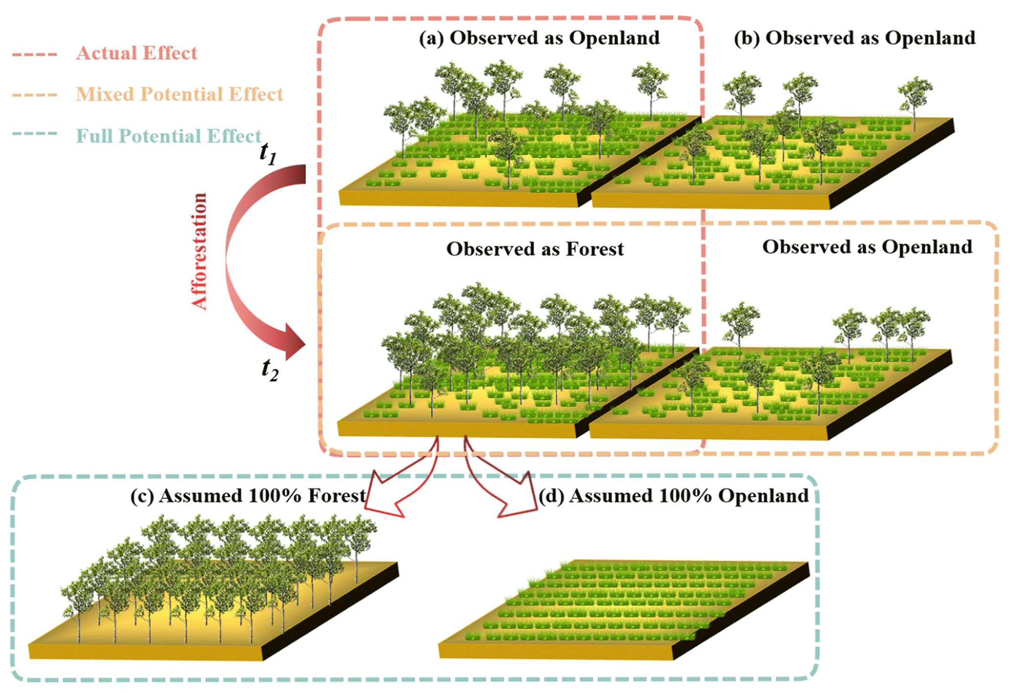
Figure 1 Illustration of the three approaches to quantifying the local surface temperature effect of afforestation. Panels (a) and (b) represent two nearby pixels, both classified as openland at time t₁ by medium-resolution satellites (1 km spatial resolution), with one of them classified as forest at time t₂ (i.e., having experienced afforestation) and the other unchanged. Note that neither of these pixels will have 100 % complete coverage of either openland (i.e., grassland or cropland) or forest, but they will have been classified as either openland or forest by medium-resolution satellite products. Panels (c) and (d) represent pixels with 100 % forest or 100 % openland coverage whose temperature can be derived from pixels of mixed land-cover types by using the singular value decomposition (SVD) technique (Duveiller et al., 2018). The dotted red box describes the quantification of the actual effect of afforestation (ΔT_a) occurring from t₁ to t₂ by the space-and-time method. The orange box represents the mixed potential effect determined by hypothesizing potential shifts between openland and forest based on the space-for-time approach ($\mathrm{\Delta }{T}_{{\mathrm{p}}_{\mathrm{1}}}$). The green box represents the full potential effect of afforestation ($\mathrm{\Delta }{T}_{{\mathrm{p}}_{\mathrm{2}}}$) derived by hypothesizing a transition from 100 % complete openland coverage to 100 % complete forest coverage.

The third method, recently used by Duveiller et al. (2018), uses the “singular value decomposition” (SVD) technique (Fig. 1, green box), which is claimed to extract the hypothetical LST for different land-cover types by assuming a 100 % coverage of the target cover type. The afforestation effect on LST is then quantified as the difference between the LST of a pixel with a hypothetical 100 % forest coverage and the LST of an adjacent pixel with 100 % openland coverage. As with the second method, such an approach quantifies the potential effect of afforestation, but in this case, it quantifies the “full potential effect” by assuming transitions between land-cover types with 100 % complete ground coverage.

Previous studies have revealed the fraction of forest change as an important factor determining the magnitude of the afforestation effect. Alkama and Cescatti (2016) indicated that the actual temperature effect is fraction-dependent, and Li et al. (2016a) pointed out that use of a higher threshold to define forest change resulted in a stronger potential effect. Nonetheless, whether the fraction of forest change can explain the differences in the afforestation effect produced by different methods, e.g., whether the potential effect can be “actualized”, has not been demonstrated. Testing the role of afforestation fraction in reconciling the afforestation effects produced by different methods can help clarify potential confusion and contribute to appropriate policy evaluation.

This study develops detailed conceptual and methodological descriptions for each of the three approaches and uses large-scale afforestation over China as a case study to compare the three approaches. We tested the following hypotheses. (1) The actual effect on LST increases with the area that has actually been afforested, defined as afforestation intensity (or F_aff). (2) The actual effect is smaller than the potential effects. (3) When extending F_aff to a hypothetical value of 100 %, the actual effect approaches the potential effect. If proven, this third hypothesis implies that the LST impacts from different approaches could be reconciled given the same boundary condition of full afforestation. In that case, we then have a fourth hypothesis (4) stating that changes in underlying biophysical processes including radiation and sensible and latent heat fluxes that drive LST changes should also be reconciled among different methods. To keep the focus on reconciling methodological differences, only changes in the daytime surface temperature were considered in this study. Nevertheless, similar conclusions regarding the different approaches are expected for nighttime surface temperature.

2 Method

2.1 Three approaches to quantifying the impacts of afforestation on LST

2.1.1 Actual effect of afforestation (ΔT_a)

The space-and-time approach assumes that the gross change in land surface temperature (ΔT) over a given time period during which afforestation occurred contains both signals of temperature change due to afforestation (ΔT_a) and background temperature variation (ΔT_res) due to changes in large-scale circulation patterns (Alkama and Cescatti, 2016; Li et al., 2016a):

$$\begin{array}{}\text{(1)}& \mathrm{\Delta }T=\mathrm{\Delta }{T}_{\mathrm{a}}+\mathrm{\Delta }{T}_{\mathrm{res}},\end{array}$$

where ΔT is the gross temperature change during the period from t₁ to t₂ for the pixel under study. ΔT can be calculated as the difference between LST${}_{t_{\mathrm{2}}}$ and LST${}_{t_{\mathrm{1}}}$, with LST${}_{t_{\mathrm{2}}}$ being the surface temperature after afforestation and LST${}_{t_{\mathrm{1}}}$ being that before afforestation. It thus follows that

$$\begin{array}{}\text{(2)}& \mathrm{\Delta }{T}_{\mathrm{a}}=\mathrm{\Delta }T-\mathrm{\Delta }{T}_{\mathrm{res}}.\end{array}$$

ΔT_res can be approximated by averaging changes in surface temperature for those pixels adjacent to the target afforestation pixel for which the forest cover remained constant between t₁ and t₂ (i.e., F_aff=0 %; Sect. 2.2.3). Here, pixels with F_aff>0 % were defined as afforestation target pixels. A searching window of 11 km × 11 km was established, centered on the afforestation pixel. Within this window, pixels with F_aff=0 % were defined as control pixels and were used to derive ΔT_res. Afforestation pixels and adjacent control pixels were both determined based on the net forest change between t₁ and t₂ using Global Forest Change (GFC) data (Fig. 2; Sect. 2.2.3).

Figure 2 Schematic overview of the processing steps. The different output results correspond to the actual effect (ΔT_a), mixed potential effect ($\mathrm{\Delta }{T}_{{\mathrm{p}}_{\mathrm{1}}}$), and full potential effect of afforestation ($\mathrm{\Delta }{T}_{{\mathrm{p}}_{\mathrm{2}}}$).

2.1.2 Mixed potential effect ($\mathrm{\Delta }{T}_{{\mathrm{p}}_{\mathrm{1}}}$)

The space-for-time method relies on the “space-substitute-for-time” assumption to obtain the potential impact of afforestation on local temperature (Zhao and Jackson, 2014). By assuming that forest and openland share the same environmental conditions (background climate, topography, etc.) within a small spatial domain, the potential temperature effect of afforestation is examined using the search window method with a window size of up to 40 km × 40 km (Ge et al., 2019; Li et al., 2015; Peng et al., 2014). Here, to be consistent with our actual effect approach, a more conservative window size of 11 km × 11 km was used, smaller than that used in the majority of previous studies (Ge et al., 2019; Li et al., 2015; Peng et al., 2014). In most previous studies, existing medium-resolution (1 km) land-cover maps were used directly. Such land-cover products rely on certain thresholds to classify satellite pixels into discrete land-cover types. Given the widespread spatial heterogeneity in land-cover distribution, it is to be expected that only in rare cases will these medium-resolution pixels have 100 % coverage of a given land-cover type. Therefore, when determined in this way, the potential effect of afforestation has been named the mixed potential effect, in contrast to the full potential effect, on which we will focus in the next section, which assumes a potential transition between land-cover types of 100 % coverage.

To ensure consistency with the land-cover data used in the full potential effect approach (i.e., the singular value decomposition method), the GlobeLand30 land-cover map was aggregated from its original resolution (30 m) to 1 km resolution. The land-cover type assigned to a given 1 km pixel during aggregation was based on the land-cover type with an area fraction >50 % within that pixel, to be consistent with the rationale behind the generation of medium-resolution land-cover products (Sect. 2.2.3). A 1 km forest pixel was then chosen as the target pixel and put at the center of a search window with dimensions 11 km × 11 km. The mixed potential effect of afforestation ($\mathrm{\Delta }{T}_{{\mathrm{p}}_{\mathrm{1}}}$) was defined as the difference between the temperature of the target pixel (LST_F) and the average temperature of all the surrounding openland pixels within the window ($\stackrel{\mathrm{‾}}{{\mathrm{LST}}_{\mathrm{O}}^{\prime }}$):

$$\begin{array}{}\text{(3)}& \mathrm{\Delta }T=\mathrm{\Delta }{T}_{{\mathrm{p}}_{\mathrm{1}}}-\stackrel{\mathrm{‾}}{{\mathrm{LST}}_{\mathrm{O}}^{\prime }},\end{array}$$

where LST_F is the surface temperature of the target forest pixel at t₂, and ${\mathrm{LST}}_{\mathrm{O}}^{\prime }$ represents the elevation-corrected surface temperature of openland pixels at t₂ within the search window. Given our search window size, $\mathrm{\Delta }{T}_{{\mathrm{p}}_{\mathrm{1}}}$ could be biased by the elevation difference between the target forest pixel and surrounding openland pixels. Therefore, a linear relationship was first fitted between the observed openland temperature, LST_O, and the elevation of the openland pixel (Ele_O). This fitted temperature lapse rate (k) was then used to derive elevation-corrected openland temperature ${\mathrm{LST}}_{\mathrm{O}}^{\prime }$:

$$\begin{array}{}\text{(4)}& {\mathrm{LST}}_{\mathrm{O}}^{\prime }={\mathrm{LST}}_{\mathrm{O}}+k\times \mathrm{\Delta }{\mathrm{Ele}}_{\mathrm{F}-\mathrm{O}},\end{array}$$

where ΔEle_F−O is the elevation difference between forest and openland pixels. The elevation is available from NASA's Shuttle Radar Topography Mission (SRTM) dataset (https://lpdaac.usgs.gov/products/srtmgl1v003/, last access: 23 December 2022).

2.1.3 Full potential effect ($\mathrm{\Delta }{T}_{{\mathrm{p}}_{\mathrm{2}}}$)

The full potential effect represents the temperature change due to hypothesizing a shift from 100 % openland to 100 % forest coverage and was determined here by employing the singular value decomposition (SVD) method used in Duveiller et al. (2018). The SVD technique assumes that the temperature observed for a pixel at 1 km scale is a linear composition of the temperatures of different land-cover types at a finer resolution (in our study at a 30 m resolution). For each 1 km pixel, the observed temperature can be written as the composition of the temperature of each component land-cover type and its corresponding fraction, based on the land-cover fractions derived from the 30 m resolution GlobeLand30 map (Sect. 2.2.3). The temperature of each type of land cover was assumed constant within a search window of 11 km × 11 km. For each given search window, the following equations can be obtained:

$$\begin{array}{}\text{(5)}& \left(\begin{array}{c}{y}_{\mathrm{1}}\\ \mathrm{⋮}\\ y_n\end{array}\right)=\left(\begin{array}{ccc}{x}_{\mathrm{11}}& \mathrm{\dots }& x_{\mathrm{1}m}\\ \mathrm{⋮}& \mathrm{\ddots }& \mathrm{⋮}\\ x_{n\mathrm{1}}& \mathrm{\cdots }& x_{nm}\end{array}\right)\times \left(\begin{array}{c}{\mathit{\beta }}_{\mathrm{1}}\\ \mathrm{⋮}\\ {\mathit{\beta }}_m\end{array}\right),\end{array}$$

where n is the total number of 1 km pixels within the window, after accounting for the elevation difference (thus the maximum value of n is 121 given our 11 km × 11 km search window), m is the number of land-cover types, x_ij refers to the fraction of land-cover type j in pixel i, and β_i refers to the temperature of land-cover type i. To minimize elevation impacts, the linear regression relationship for a given 1 km pixel was included only when the elevation difference between this pixel and the central pixel of the search window was smaller than 100 m. Using matrix notation, Eq. (5) can be simplified to

$$\begin{array}{}\text{(6)}& y=\mathbf{X}\times \mathit{\beta },\end{array}$$

where the matrix X contains land-cover fraction for the n 1 km pixels as an explanatory variable, the response variable y contains n LST observations, and the coefficient vector, β, contains the regression coefficients which show temperatures of different land-cover types. Note that this linear equation system cannot be easily solved because the matrix X is “closed”; i.e., by definition, the elements in each row of the matrix X add up to 1. After removing the mean of each column (Zhang et al., 2007), the matrix X was transformed by applying the SVD technique to another matrix, Z, of reduced dimension (more details in Duveiller et al., 2018). After this transformation, we have the following:

$$\begin{array}{}\text{(7)}& y=\mathbf{Z}\times {\mathit{\beta }}^{\prime }+\mathit{\epsilon }\end{array}$$

in which the β^′ coefficient can be obtained from Eq. (8):

$$\begin{array}{}\text{(8)}& {\mathit{\beta }}^{\prime }={\left({\mathbf{Z}}^t\mathbf{Z}\right)}^{-\mathrm{1}}{\mathbf{Z}}^{t}y.\end{array}$$

However, the β^′ vector calculated from the transformed matrix Z cannot directly provide surface temperatures for corresponding land-cover types. To obtain temperatures for each land-cover type by assuming 100 % ground coverage, an identity matrix Y with its dimension equal to the number of land-cover types must be constructed to represent the hypothetical case in which each 1 km pixel was 100 % covered by a single land-cover type. The same transformation as applied to the matrix X was then applied to Y, to obtain a transformed matrix Z^′. Finally, the predicted temperature (${\mathrm{LST}}_{\mathrm{100}\mathit{\%}}^{\prime }$) for each land-cover type assuming a 100 % coverage is calculated as

$$\begin{array}{}\text{(9)}& {\mathrm{LST}}_{\mathrm{100}\mathit{\%}}^{\prime }={\mathbf{Z}}^{\prime }{\mathit{\beta }}^{\prime }.\end{array}$$

For the central pixel of the local search window, $\mathrm{\Delta }{T}_{{\mathrm{p}}_{\mathrm{2}}}$ is defined as the difference between the predicted ${\mathrm{LST}}_{\mathrm{100}\mathit{\%}}^{\prime }$ for forest (${\mathrm{LST}}_{\mathrm{100}\mathit{\%}\mathrm{F}}^{\prime }$) and openland (${\mathrm{LST}}_{\mathrm{100}\mathit{\%}\mathrm{O}}^{\prime }$).

$$\begin{array}{}\text{(10)}& \mathrm{\Delta }{T}_{{\mathrm{p}}_{\mathrm{2}}}={\mathrm{LST}}_{\mathrm{100}\mathit{\%}\mathrm{F}}^{\prime }-{\mathrm{LST}}_{\mathrm{100}\mathit{\%}\mathrm{O}}^{\prime }\end{array}$$

More details, including an illustration of the SVD method, can be found in Fig. 7 in Duveiller et al. (2018).

At the scale of the searching windows used in this analysis (11 km × 11 km), any nonlocal effects cancel out when comparing temperature differences over neighboring areas because the effects of advection and atmospheric circulation have been reported to be similar for adjacent areas (Pongratz et al., 2021; Winckler et al., 2019a). Hence the quantified afforestation effect for each of the three methods can be considered to be the local effect only.

2.2 Dataset and processing

2.2.1 The test case: large-scale afforestation over China

China was selected as the test case for addressing the important methodological issues in quantifying land surface impacts of afforestation because afforestation is a key national strategy for sustainable development and climate mitigation (Bryan et al., 2018; Qi and Wu, 2013). According to the 8th National Forest Inventory conducted in 2013, China's afforestation area has reached 69×10⁶ ha, accounting for 33 % of the total global afforestation area (Chen et al., 2019). Afforestation in China during 2000–2012 occurred mainly in regions with more than 400 mm of precipitation per year (Fig. 3a), which is considered a threshold below which there is a high risk of afforestation failing due to water limitation (Mátyás et al., 2013). China covers a wide range of latitude from 3.9 to 53.6^∘ N, and its forest ecosystems cover an elevation range of 100 to 4000 m. This wide range of climate zones, from tropical/subtropical to temperate and boreal, makes it highly suitable for our methodological analysis because the impact of afforestation on LST might differ with latitude and background climate (Lee et al., 2011; Alkama and Cescatti, 2016). Further justification for using China as a test case comes from the strongly diverging published LST impacts of afforestation there, which range from an actual effect of −0.0036 K per decade by Li et al. (2020) to a potential effect of −1.1 K by Peng et al. (2014).

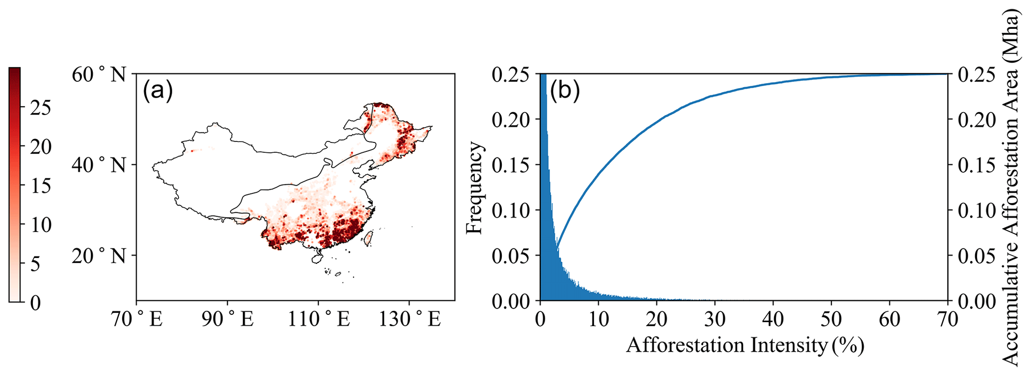
Figure 3 (a) Spatial distribution of afforestation intensity (F_aff) in China during 2000–2012. The solid black line crossing China is the 400 mm annual precipitation isoline. (b) Frequency distribution of F_aff and cumulative afforestation area with the increase in F_aff. The dashed red line represents the cumulative afforestation area corresponding to F_aff=10 %.

2.2.2 MODIS dataset and preparation

In this study, the actual effect was estimated by combining the actual satellite-derived afforestation for 2000 to 2012 (see Sect. 2.2.3) with satellite-based estimates of biophysical variables for the periods 2002–2004 (t₁) and 2010–2014 (t₂). MODIS remote sensing products for land surface temperature (MOD11A2), albedo (MCD43B3), and evapotranspiration (MOD16A2) were used to characterize the biophysical effects (Table 1). The datasets were regridded to harmonize with spatial (1 km) and temporal (annual) resolutions (Table 1).

Table 1 Summary of the datasets and their main characteristics.

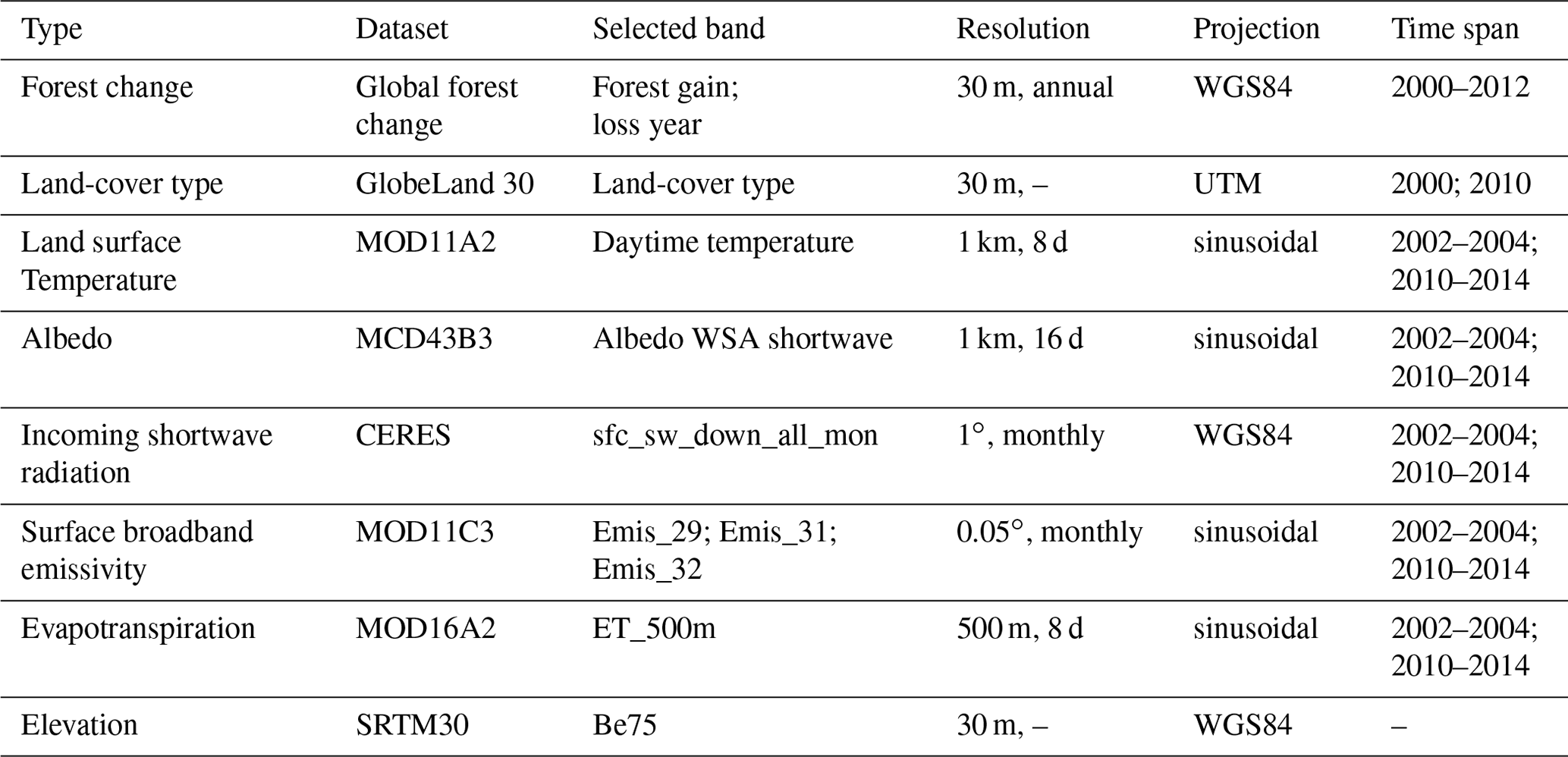
The MOD11A2 product provides 8 d land surface temperature for 10:30 and 22:30 from the Terra satellite, but here we focused on daytime surface temperature. Only valid LST observations from the original data were used to compute the average daily values for a given year. Years for which more than 40 % of daily data are missing were excluded from the analysis. Annual data were then aggregated to obtain the average annual temperature for periods t₁ and t₂.

The MCD43B3 product provides white-sky and black-sky shortwave albedo at 16 d temporal resolution (Table 1). The observed white-sky albedo was used as the daytime albedo (Peng et al., 2014). For evapotranspiration (ET), we used the ET band in MOD16A2, which includes water fluxes from soil evaporation, wet canopy evaporation, and plant transpiration. To calculate the mean annual albedo and evapotranspiration for 2002–2004 (t₁) and 2010–2014 (t₂), we used the same approach as used for LST.

2.2.3 Land-cover datasets and processing

Two land-cover datasets were used in this study: the actual effect approach was based on the Global Forest Change (GFC) dataset, while the mixed potential effect and full potential effect used the GlobeLand30 land-cover data (Table 1).

The SVD technique, used in the full potential effect approach, requires a land-cover map with a higher spatial resolution than the 1 km spatial resolution of the LST data. The GlobeLand30 product, which is based on Landsat images, provides land-cover information for China at a 30 m resolution for the years 2000 and 2010 (Chen et al., 2015). Cultivated land and grassland in GlobeLand30 were classified as openland. Discrete land-cover type information at 30 m resolution in 2010 was aggregated to obtain the area fractions of the different land-cover types at 1 km resolution, which were then used to construct matrix X in Eq. (5) (Fig. 2). Furthermore, land-cover type information at the 1 km scale was extracted, based on the vegetation type with area fraction >50 % for every 1 km × 1 km window. These data were then applied in the space-for-time method to identify forest and openland (Fig. 2).

GlobeLand30 data are not suitable for detecting forest change (Zeng et al., 2021). The Global Forest Change (GFC) data, however, provide forest gain and forest loss at a spatial resolution of 30 m between 2000 and 2012 and have been used for mapping global forest change (Hansen et al., 2013). This product shows an overall accuracy of greater than 99 % for areas of forest gain at the global scale when compared with statistical data reported in Forest Resource Assessment (FRA), lidar detection (Geoscience Laser Altimeter System), and MODIS NDVI time series (Hansen et al., 2013) and thus has been recommended for use in forest and forest-change estimates (Chen et al., 2020; Zeng et al., 2021). Using this dataset, forest loss events were identified for each year between 2000 and 2012, but forest gain was only identified for the whole period, simply because forest loss is an abrupt change which can be effectively identified over short time periods, whereas forest gain is a gradual change which can only be confidently identified over longer time spans. Here, forest losses and gains from GFC were aggregated at a 1 km resolution to obtain net forest change (defined as forest gain minus forest loss) during this period (Fig. 2). A positive net change indicates afforestation, and the area percentage of afforestation for the 1 km pixel area was defined as F_aff. The land-cover type of pixels with F_aff=0 % was considered to be stable. This net forest-change information was then used in the calculation of the actual afforestation-induced temperature effect (ΔT_a) (Fig. 2).

2.3 Decomposition of changes in surface temperature

Changes in surface temperature following forest-cover change are the net result of changes in underlying fluxes that collectively determine the land surface energy balance:

$$\begin{array}{}\text{(11)}& \begin{array}{rl}& \mathrm{\Delta }{\mathrm{SW}}_{\mathrm{in}}-\mathrm{\Delta }{\mathrm{SW}}_{\mathrm{out}}+\mathrm{\Delta }{\mathrm{LW}}_{\mathrm{in}}-\mathrm{\Delta }{\mathrm{LW}}_{\mathrm{out}}\\ & =\mathrm{\Delta }H+\mathrm{\Delta }\mathit{LE}+\mathrm{\Delta }G,\end{array}\end{array}$$

where ΔSW_in, ΔSW_out, ΔLW_in, and ΔLW_out are the changes in incoming and outgoing shortwave and longwave radiation, respectively, and ΔH, ΔLE, and ΔG are changes in sensible heat flux, latent heat flux, and ground heat flux, respectively. All the terms of Eq. (11) are expressed in watts per square meter (W m⁻²).

Firstly, it can be reasonably assumed that ΔSW_in≈0 and ΔLW_in≈0, given that all three approaches consider only local effects on surface temperature by following a comparison of target pixels with surrounding control pixels, thus excluding feedbacks from, e.g., cloud formation (Duveiller et al., 2018). Changes in reflected shortwave radiation can be derived as

$$\begin{array}{}\text{(12)}& \mathrm{\Delta }{\mathrm{SW}}_{\mathrm{out}}={\mathrm{SW}}_{\mathrm{in}}\times \mathrm{\Delta }\mathit{\alpha },\end{array}$$

where SW_in is available from the CERES EBAF surface product Ed 4.1 (Kato et al., 2018; Liu et al., 2018) (Table 1), and Δα is the surface albedo change. To approximate ΔLW_out, we used its first-order differential equation:

$$\begin{array}{}\text{(13)}& \mathrm{\Delta }{\mathrm{LW}}_{\mathrm{out}}=\mathit{\sigma }(\mathrm{4}{\mathit{\epsilon }}_{\mathrm{B}}{T}^{\mathrm{3}}\mathrm{\Delta }T+\mathrm{\Delta }{\mathit{\epsilon }}_{\mathrm{B}}{T}^{\mathrm{4}}),\end{array}$$

where σ is Stefan–Boltzmann's constant ($\mathrm{5.67}\times {\mathrm{10}}^{-\mathrm{8}}$ W m⁻² K⁻⁴), T is daytime surface temperature, and ΔT is the afforestation impact on surface temperature. Surface broadband emissivity, ε_B, is usually obtained from an empirical relationship (Zhang et al., 2020):

$$\begin{array}{}\text{(14)}& {\mathit{\epsilon }}_{\mathrm{B}}=\mathrm{0.2122}{\mathit{\epsilon }}_{\mathrm{29}}+\mathrm{0.3859}{\mathit{\epsilon }}_{\mathrm{31}}+\mathrm{0.4029}{\mathit{\epsilon }}_{\mathrm{32}},\end{array}$$

where ε₂₉, ε₃₁, and ε₃₂ are obtained from the estimated emissivity for bands 29 (8400–8700 nm), 31 (10 780–11 280 nm), and 32 (11 770–12 270 nm) in the MOD11C3 data (Duveiller et al., 2018).

Latent heat flux change (ΔLE) refers to changes in the energy used for evapotranspiration (ET, unit: mm d⁻¹), which can be obtained from the change in evapotranspiration (ΔET):

$$\begin{array}{}\text{(15)}& \mathrm{\Delta }\mathit{LE}=\mathrm{\Delta }\mathrm{ET}\times \mathrm{28.94}\mathrm{W}{\mathrm{m}}^{-\mathrm{2}}(\mathrm{mm}{\mathrm{d}}^{-\mathrm{1}}{)}^{-\mathrm{1}}.\end{array}$$

Therefore, the sum of sensible heat change and ground heat change (ΔH+ΔG) can be calculated as the difference between net radiation change and latent heat flux change (ΔLE) based on Eq. (11). The afforestation effects on albedo (Δα), ε_B (Δε_B), and ET (ΔET) needed in the above equations were calculated in a similar way to ΔT for each of the three different approaches as described in Sect. 2.1.

2.4 Statistical analysis

The spatial distributions of original samples for the three methods are different because of the different land-cover maps used (Figs. 2 and A1 in Appendix A), and, therefore, the statistical analysis was limited to those pixels shared by all three approaches: 96 058 sample pixels at 1 km resolution. The distribution of these shared sample pixels retained the characteristics of the spatial distribution of the original samples (Fig. A2).

Differences in the afforestation effects on LST of the three approaches were tested by performing paired-sample t tests between pairs of approaches. The paired-sample t test was used, rather than a normal t test, to avoid the bias due to strong spatial heterogeneity in the LST effects of afforestation that could occur if the values of all pixels had been pooled together for a normal t test. The test was done using the “ttest_rel” method from the “scipy.stats” package in Python. The Bonferroni correction was applied to adjust the significance level (p value) to mitigate the increasing type I error when doing multiple paired-sample t tests, which in our case involves three pairs (Lee and Lee, 2018; UC Berkeley, 2008). The Bonferroni correction sets the significance cutoff at $\mathit{\alpha }/k$ (with α as the p value before correction and k as number of pairs). In this study, with three hypotheses tests (i.e., three pairs) and an original significance level α=0.05, the adjusted p value is 0.0167. In order to investigate ΔT_a in relation to the afforestation intensity, a linear regression was performed between ΔT_a and F_aff using the ordinary least-squares method.

3 Results

3.1 Spatial distribution of afforestation and its effect on land surface temperature

In China, afforestation areas are mainly located in the northeast, southwest, and south, where sufficient precipitation is available (Fig. 3a) and largely driven by afforestation of former cropland or abandoned cropland, with a relatively small contribution from forest regeneration or replanting following natural disturbance or timber harvest. One prominent feature of afforestation in China is its small afforestation patch, with most afforested pixels (1 km²) having an afforestation fraction of less than 30 % (Fig. 3b). Pixels with an afforestation intensity below 10 % account for 93 % of the total number of pixels (Fig. 3b), representing 0.14×10⁶ ha, more than half (55.6 %) of the total afforestation area (Fig. 3b).

Although all three approaches result in similar spatial and latitudinal patterns regarding afforestation effects on LST (Fig. 4), their magnitudes differ substantially. The actual effect has the lowest temperature change, followed by the mixed potential effect, with the full potential effect showing the greatest temperature change (Fig. 4a–c). For the latitude range of 20–36^∘ N where afforestation effects show a dominant cooling effect, the full potential effect ($\mathrm{\Delta }{T}_{{\mathrm{p}}_{\mathrm{2}}}$) reaches $-\mathrm{1.75}\pm \mathrm{0.01}$ K, while the mixed potential effect ($\mathrm{\Delta }{T}_{{\mathrm{p}}_{\mathrm{1}}}$) was smaller at $-\mathrm{0.96}\pm \mathrm{0.00}$ K, but both of them were much larger than the actual effect (ΔT_a) of $-\mathrm{0.09}\pm \mathrm{0.00}$ K. Similarly, the full potential effect ($\mathrm{\Delta }{T}_{{\mathrm{p}}_{\mathrm{2}}}$) showed the strongest warming effect (0.35±0.01 K) in the area north of 48^∘ N, stronger than the mixed potential effect (0.22±0.01 K), and again the actual effect is the smallest (0.07±0.01 K). However, regarding the latitude where the effects change from a warming to cooling effect, the three approaches largely converge (Fig. 4d). Between 40 and 48^∘ N, the afforestation effects are largely neutral, with the mean temperature change for the three approaches being 0.07±0.01 K ($\mathrm{\Delta }{T}_{\mathrm{a}}=-\mathrm{0.01}\pm \mathrm{0.01}$ K; $\mathrm{\Delta }{T}_{{\mathrm{p}}_{\mathrm{1}}}=\mathrm{0.11}\pm \mathrm{0.01}$ K; $\mathrm{\Delta }{T}_{{\mathrm{p}}_{\mathrm{2}}}=\mathrm{0.12}\pm \mathrm{0.01}$ K).

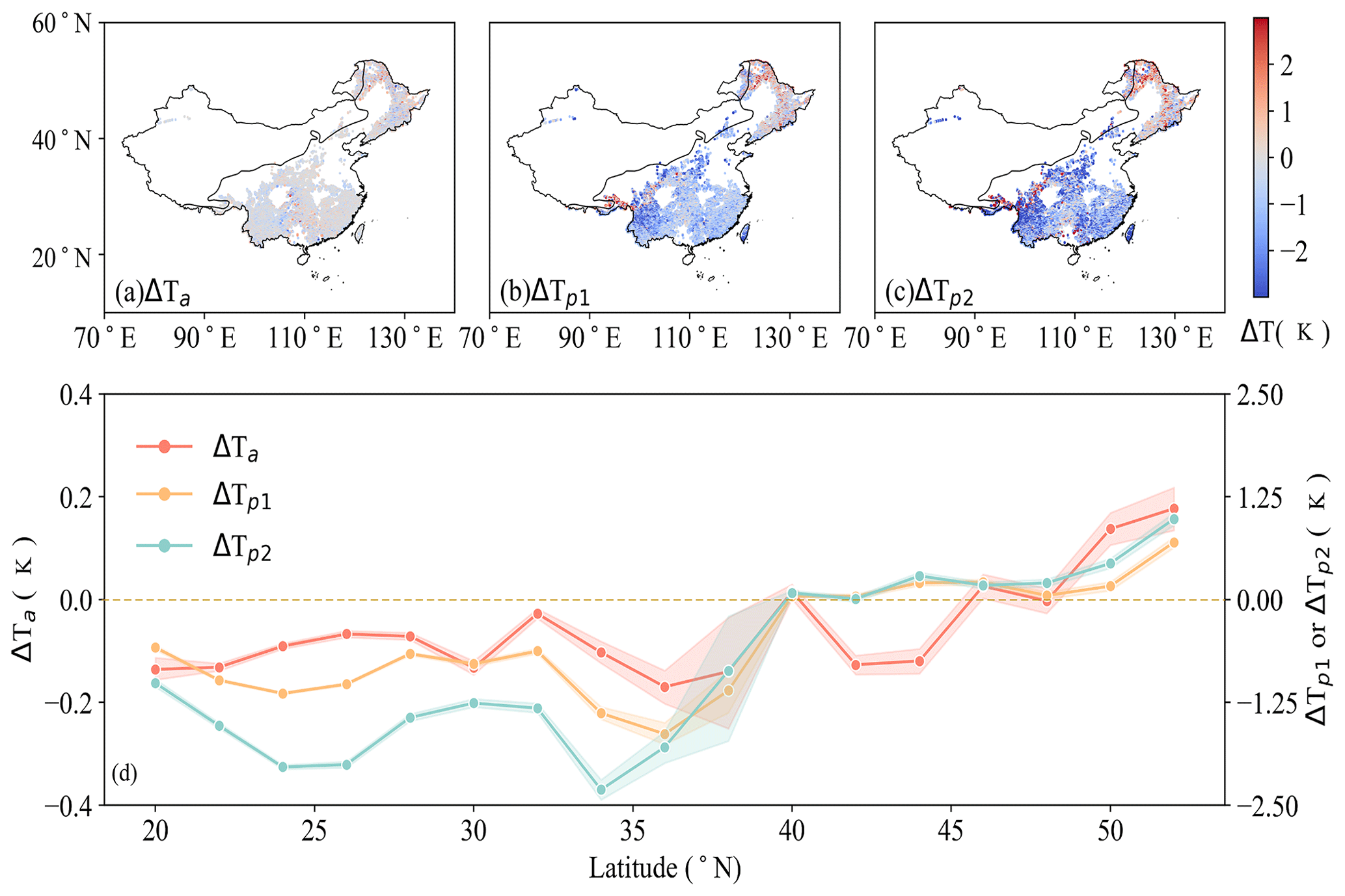
Figure 4 Afforestation effects on LST quantified by three approaches: (a) actual effect based on a space-and-time approach (ΔT_a), (b) mixed potential effect based on a space-for-time approach ($\mathrm{\Delta }{T}_{{\mathrm{p}}_{\mathrm{1}}}$), and (c) full potential effect assuming a transition from 100 % openland coverage to 100 % forest coverage using the SVD method ($\mathrm{\Delta }{T}_{{\mathrm{p}}_{\mathrm{2}}}$). The solid black line crossing China is the 400 mm precipitation isoline. (d) Zonal averages of the annual mean daytime LST change within 2^∘ latitudinal bins, with shaded areas representing the standard errors (SE). Note that in (d), ΔT_a corresponds to the vertical axis on the left; $\mathrm{\Delta }{T}_{{\mathrm{p}}_{\mathrm{1}}}$ and $\mathrm{\Delta }{T}_{{\mathrm{p}}_{\mathrm{2}}}$ correspond to the vertical axis on the right.

3.2 Reconciling temperature effects of afforestation

Even though the observed land surface temperature is assumed to be uniform for the 1 km afforested satellite pixel, the underlying afforestation intensity varies substantially (Fig. 3a). This leads to our first hypothesis that for a 1 km pixel, ΔT_a should be influenced by the area fraction that has been afforested within the pixel (i.e., afforestation intensity or F_aff). Indeed, the actual daytime surface cooling increases significantly with afforestation intensity (Fig. 5), with a 0.079±0.017 K (mean ± SD) increase for each 10 % increase in F_aff.

Figure 5 Changes in ΔT_a as a function of afforestation intensity (F_aff), defined as the fraction of afforested area to the total pixel area at a 1 km resolution. Error bars indicate the standard error of ΔT_a within each 10 % bin of F_aff. The red line represents the fitted linear regression line between ΔT_a and F_aff.

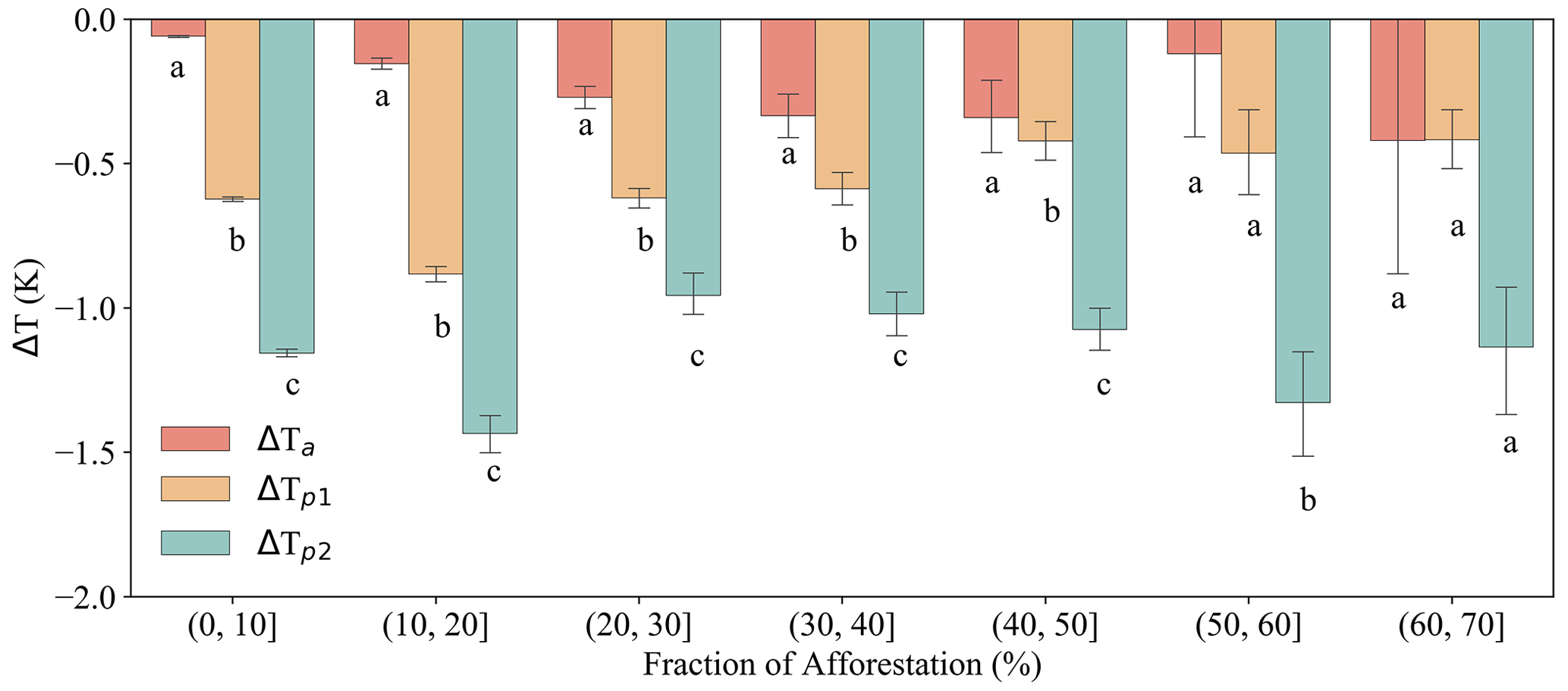
Figure 6 Comparison of ΔT for the three approaches for bins of afforestation intensity. Error bars are given as the standard error, and different letters indicate that ΔT calculated by the two approaches concerned are significantly different using the adjusted p value after applying the Bonferroni correction for multiple paired-sample t tests.

The afforestation effects obtained from the three approaches were compared for each F_aff interval (Fig. 6). When afforestation intensity is less than 60 %, significant differences exist in the temperature change obtained by the three approaches, with $\mathrm{\Delta }{T}_{\mathrm{a}}<\mathrm{\Delta }{T}_{{\mathrm{p}}_{\mathrm{1}}}<\mathrm{\Delta }{T}_{{\mathrm{p}}_{\mathrm{2}}}$. This result confirms our second hypothesis that the actual effect is expected to be smaller than potential effects. However, for pixels with relatively low F_aff, the mixed potential effect is found to be smaller than the full potential effect, which is reasonable but, to our knowledge, has not been reported before. When the afforestation intensity is greater than 60 %, the significant difference in cooling effect between the different approaches disappears, likely because afforestation intensity and the associated forest coverage at 1 km resolution reach values high enough to allow the potential effects to be realized.

When considering the overall differences in ΔT for the three approaches, irrespective of the afforestation intensity, ΔT_a ($-\mathrm{0.07}\pm \mathrm{0.00}$ K) over China was significantly lower than $\mathrm{\Delta }{T}_{{\mathrm{p}}_{\mathrm{1}}}$ ($-\mathrm{0.63}\pm \mathrm{0.00}$ K), which is further significantly lower than $\mathrm{\Delta }{T}_{{\mathrm{p}}_{\mathrm{2}}}$ ($-\mathrm{1.16}\pm \mathrm{0.01}$ K) (p<0.05, paired-sample t test, n = 96 058), once again confirming our second hypothesis (Fig. 7). Moreover, extrapolation of the relationship shown in Fig. 5 suggests that ΔT_a would reach $-\mathrm{0.79}\pm \mathrm{0.17}$ K (mean ± SD) if a 1 km pixel was 100 % afforested, which is conceptually comparable to the potential effects. ΔT_a was indeed found to be higher than $\mathrm{\Delta }{T}_{{\mathrm{p}}_{\mathrm{1}}}$ but lower than $\mathrm{\Delta }{T}_{{\mathrm{p}}_{\mathrm{2}}}$. This result confirms our third hypothesis and demonstrates that the potential cooling effect could indeed be reached when a pixel is fully afforested.

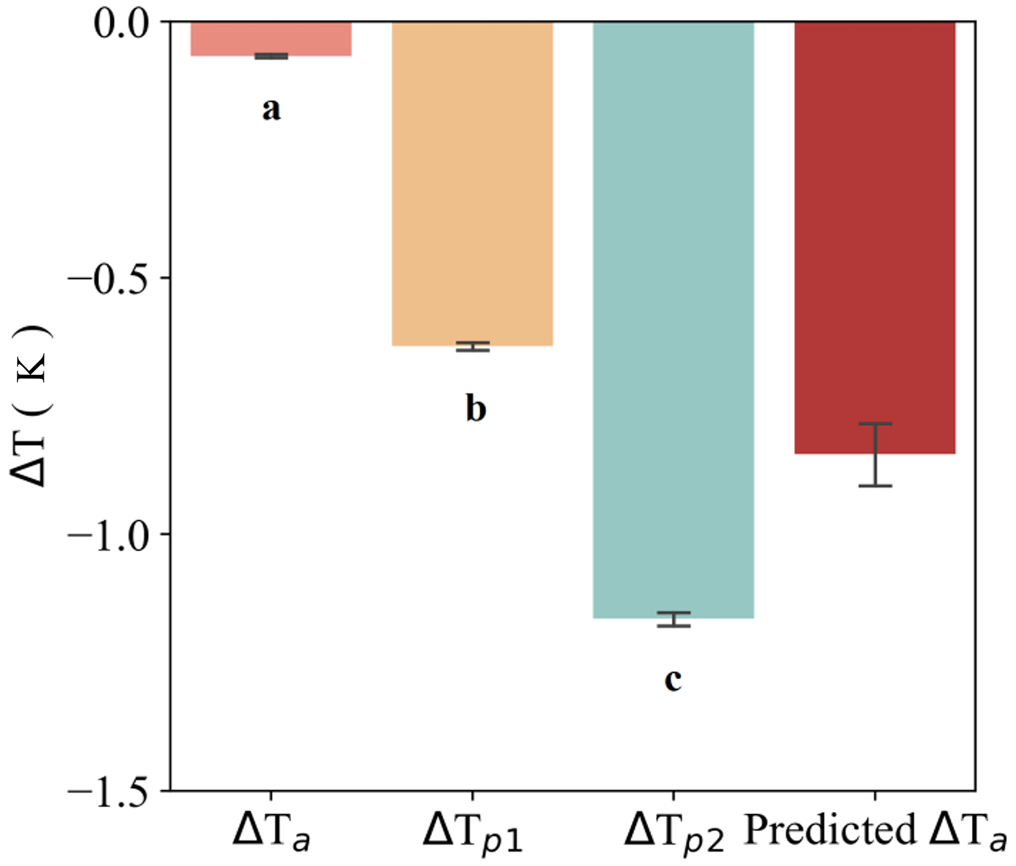
Figure 7 Comparison of ΔT for the three approaches, irrespective of the afforestation intensity. Error bars are given as the standard error, and different letters indicate ΔT being significantly different (p=0.0167, paired-sample t test, n = 96 058). For comparison, the predicted ΔT_a with F_aff reaching 100 %, which is conceptually comparable with $\mathrm{\Delta }{T}_{{\mathrm{p}}_{\mathrm{1}}}$ and $\mathrm{\Delta }{T}_{{\mathrm{p}}_{\mathrm{2}}}$, is also shown.

3.3 Reconciling changes in surface energy fluxes by afforestation

In order to investigate whether the underlying surface energy fluxes could be reconciled following the reconciliation of the LST changes, changes in surface energy fluxes due to afforestation were quantified using each of the three approaches, under the same boundary conditions as for full afforestation (i.e., changes following the actual effect approach were extended for F_aff=100 %). As illustrated in Fig. 8, changes in all the relevant surface energy fluxes under the three different approaches have the same direction, with similar magnitudes, confirming the reconciliation of the different approaches in terms of surface energy fluxes. More specifically, the three approaches converge on a reduction in reflected shortwave radiation (ΔSW_out) of 0.56–1.23 W m⁻² due to the lower albedo of forest compared to openland (Fig. A3). Emitted longwave radiation (ΔLW_out) was reduced by 1.03–3.10 W m⁻², and sensible and ground heat fluxes (ΔH+ΔG) reduced by 4.84–6.14 W m⁻². All these reduced fluxes were offset by an increased latent heat flux of 7.99–8.41 W m⁻² (ΔLE), the single energy flux leading to surface cooling.

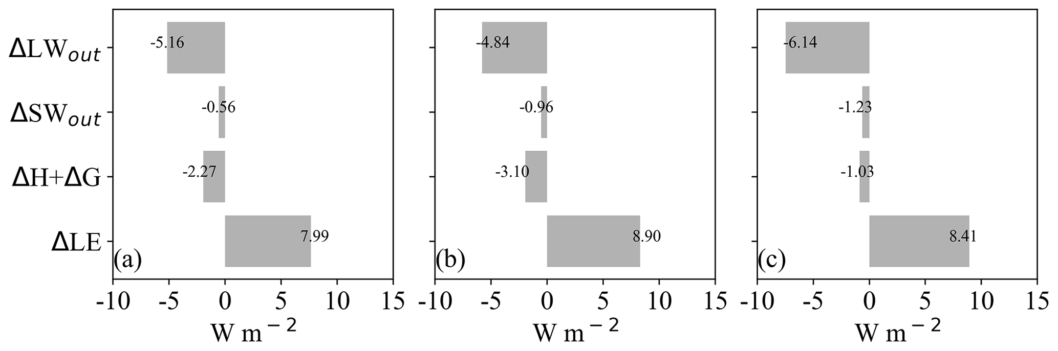
Figure 8 Afforestation-induced changes in surface energy fluxes (W m⁻²) following the three approaches: (a) the actual effect based on a space-and-time approach, (b) the mixed potential effect using medium-resolution land-cover maps based on a space-for-time approach, and (c) the full potential effect assuming a transition from 100 % openland coverage to 100 % forest coverage using the SVD method. For each approach, changes were calculated for the reflected shortwave radiation (SW_out), outgoing longwave radiation (LW_out), latent heat flux (LE), and the combination of sensible and ground heat fluxes (H+G). No changes were assumed for incoming shortwave and longwave radiation. Changes in energy fluxes for the actual effect approach have been adjusted to the condition of full afforestation (i.e., F_aff=100 %) in a similar way as for the predicted ΔT_a in Fig. 7, by fitting linear regressions between energy flux variables and F_aff (Fig. A4).

4 Discussion

The three approaches (Li et al., 2015; Alkama and Cescatti, 2016; Duveiller et al., 2018) used to quantify local surface temperature change following forest-cover change and presented in detail in this study have been cited over 919 times in research papers (Web of Science, December 2021) and in high-level climate science synthesis reports. Despite the apparently large differences in temperature effect among them, to our knowledge, no studies have examined whether these differences can be reconciled. This study fills that gap by comparing the three approaches for a single study case, i.e., large-scale afforestation in China. China is highly suitable for the purpose of this study as the size of an afforestation patch is, in general, smaller than the spatial resolution (1 km) at which the temperature effects of afforestation were conducted in the previous studies describing the three approaches (Li et al., 2015; Alkama and Cescatti, 2016; Duveiller et al., 2018). Hence, the difference between the actual and potential temperature effects is expected to be large.

Indeed, we found surface cooling following afforestation was much less when estimated as the actual effect (ΔT_a) compared to the potential effects ($\mathrm{\Delta }{T}_{{\mathrm{p}}_{\mathrm{1}}}$ and $\mathrm{\Delta }{T}_{{\mathrm{p}}_{\mathrm{2}}}$). This lower ΔT_a has been attributed to incomplete afforestation at a 1 km resolution, at which potential effects are quantified by assuming complete afforestation (i.e., a complete shift from openland to forest). Consistent with our first hypothesis, the afforestation fraction at a 1 km resolution explained 89 % of the variation in ΔT_a, making it a key determinant of the surface cooling following afforestation (Fig. 5). This result is consistent with the fact that the observed temperature for a mixed surface is determined by the area fractions of its respective components, with each component having a unique temperature. This fact also forms the theoretical foundation for the SVD technique used to derive the full potential effect (Duveiller et al., 2018).

Modeling (Li et al., 2016b) and satellite-based (Alkama and Cescatti, 2016) studies have found that temperature change after afforestation (or deforestation) is highly sensitive to the fraction of the model grid cell or satellite pixel that is subjected to afforestation (or deforestation), echoing our finding that ΔT_a significantly changes with F_aff. In addition, we provide strong evidence in support of our third hypothesis that when F_aff reaches 100 %, the expected actual effect is comparable to the potential effects (Fig. 7). This finding shows that the three approaches compared here are consistent when the same boundary condition, i.e., full afforestation, is applied and demonstrates that all three methods are mutually compatible. It is, therefore, the basis of the reconciliation of the three approaches. It also highlights the fact that the actual afforestation area must be considered when evaluating the climate mitigation effects of afforestation.

Our results also show that the mixed potential effect ($\mathrm{\Delta }{T}_{{\mathrm{p}}_{\mathrm{1}}}$) is smaller than the full potential effect ($\mathrm{\Delta }{T}_{{\mathrm{p}}_{\mathrm{2}}}$) (Figs. 6, 7). We suspect that this phenomenon likely also relates to the incomplete forest coverage for the identified forest pixels at the 1 km scale used in the space-for-time analysis because a threshold value of 50 % forest cover was used when upscaling the 30 m land-cover map to 1 km resolution. This threshold, however, is consistent with the commonly applied value in land-cover classification based on medium-resolution satellite images, such as MCD12Q1, which uses a tree coverage value of 60 % to identify forest pixels (Sulla-Menashe et al., 2019). For the purpose of comparison, we also calculated the mixed potential effect based on the MCD12Q1 land-cover map but using the same LST data. The result shows that potential effects derived using MCD12Q1 data versus those derived using spatially upscaled GlobeLand30 data are almost identical (Fig. A5), lending credibility to our estimated $\mathrm{\Delta }{T}_{{\mathrm{p}}_{\mathrm{1}}}$ in comparison to previous studies using MODIS land-cover data (Li et al., 2015). Progressively increasing the forest-cover threshold from 50 % to 90 % steadily increases $\mathrm{\Delta }{T}_{{\mathrm{p}}_{\mathrm{1}}}$ from $-\mathrm{0.62}\pm \mathrm{0.02}$ to $-\mathrm{0.75}\pm \mathrm{0.02}$ K (Fig. A6). Further increasing the thresholds used to identify 1 km resolution openland pixels from 50 % to 90 % increases $\mathrm{\Delta }{T}_{{\mathrm{p}}_{\mathrm{1}}}$ from $-\mathrm{0.63}\pm \mathrm{0.00}$ to $-\mathrm{1.10}\pm \mathrm{0.02}$ K (Fig. A7), bringing $\mathrm{\Delta }{T}_{{\mathrm{p}}_{\mathrm{1}}}$ even closer to $\mathrm{\Delta }{T}_{{\mathrm{p}}_{\mathrm{2}}}$ ($-\mathrm{1.16}\pm \mathrm{0.01}$ K). This is consistent with the finding of a previous study on the dependence of the temperature effect on the forest-cover-change thresholds that were used to define afforestation: the higher the threshold, the stronger the impact on temperature (Li et al., 2016). Our results add further support to the compatibility of the three approaches given the same boundary condition, i.e., the complete transformation from full openland to full forest coverage.

Several factors may contribute to the remaining differences in the temperature effects produced by different methods even after reconciliation. As described in the Method section, there are discrepancies in the assumptions of the three approaches, which lead to differences in the control pixels (i.e., adjacent comparison pixels). For instance, for the “pure” potential effect, it is assumed that the LSTs for pixels with the same land-cover type are uniform, and forest pixels are compared with openland pixels, whereas in the mixed potential effect approach, the central target forest pixel is compared with the mean value of non-forest pixels within the searching window. Moreover, space-for-time is an assumption that cannot be verified (Chen and Dirmeyer, 2016) and which will inevitably result in differences in the estimated actual and potential effects, although the consistency between potential and “actual” effects after reconciliation in our study does illustrate the broad validity of this assumption.

Differences between the actual and potential temperature effects can also arise from influences of both the timing of the afforestation and the time period elapsed following afforestation. However, such influences are expected to be small in our study. We argue that such influences should be more pronounced in the case of deforestation than afforestation. The temperature effect caused by deforestation is considered to be instant (Liu et al., 2018). As a result, if deforestation occurred in 1 specific year of our starting time window (i.e., 2002–2004), using the time-averaging LST over the whole time window to represent the LST before deforestation will greatly bias the quantified ΔT. In contrast, afforestation-driven surface temperature change can only gradually increase with forest development. The LST effect depends on different stages of forest development and is expected to saturate only when the forest canopy stabilizes (Zhang et al., 2021; Windisch et al., 2021). Observation studies show that closed dense-canopy old forests can exert a greater cooling effect than the open-canopy young forests (Zhang et al., 2021; Windisch et al., 2021; Duveiller et al., 2018, 2020). Hence, given the gradual nature of the afforestation effect on LST, when we quantify the afforestation effect by comparing the time-averaging LST before and after afforestation, the influence of the specific timing of afforestation is expected to be small. Furthermore, the GFC dataset used in this analysis defined forest gain using the condition of successful detection of a stable closed forest canopy that is clearly different from a non-forest state (Hansen et al., 2013), which enhances the chance of temperature change saturation following afforestation. But, given a maximum stand age of 12 years inferred from the GFC dataset, differences in surface temperatures may still exist between newly established forests and the mature existing forests that were used in the potential effect approaches. Thus, we cannot exclude the possible contribution of time period elapsed following afforestation to the difference between the actual and potential effects, which failed to be reconciled.

Previous analyses have documented latitudinal patterns of surface temperature change induced by afforestation (Alkama and Cescatti, 2016; Li et al., 2015, 2016a; Peng et al., 2014). When comparing the three approaches for a single case study, consistent latitudinal patterns of local surface temperature effects following afforestation are observed (Fig. 4). Notably, all three approaches show a warming effect in the northern high latitudes and an opposite cooling effect in the southern low latitudes, with a largely neutral effect in the 40–48^∘ N latitude band, providing further evidence that the three approaches are compatible. In particular, although the three approaches used different land-cover maps, they derived consistent LST impacts following afforestation, which highlights that fact that the reconciliation provided in this study is rather robust and unlikely to be dependent on the land-cover datasets used.

In addition to the reconciliation of the land surface temperature change, we checked and confirmed that the changes in surface energy fluxes that underlie and drive the changes in surface temperature are compatible under the boundary condition of full afforestation. This finding confirms the inherent consistency in the three approaches and clarifies the reasons behind the apparent discrepancies in existing studies as discussed in the Introduction. Nonetheless, when it comes to the biophysical impacts of afforestation in the real world, our findings have far-reaching implications. Full afforestation is often possible at small spatial scales but becomes challenging at large scale. Therefore, the realization of the full potential effect by afforestation is scale-dependent. For example, a complete afforestation of the semi-arid Loess Plateau in the northwest of China is predicted to generate a surface cooling effect of 2.40±0.07 K, but substantial afforestation efforts over the past 4 decades in that region have only realized a cooling of 0.11±0.01 K, as measured by the actual effect. Because of greater water consumption by forest compared to openland and the need to maintain land area for food production, achieving the full cooling potential may not be feasible (Huang et al., 2018; Liu and She, 2012; Liang et al., 2019).

Potential cooling effects have a value in that they can serve to establish the envelope of effects and measure possible outcomes given the condition of full afforestation. However, given the challenge of full afforestation at large spatial scales, potential effects should be converted into a more realistic estimate (i.e., actual effects), by taking into account the intensity of afforestation, to better represent policy ambitions. The analog could also be made for the effects of the surface energy impacts of afforestation. Taking 10 % as the afforestation intensity threshold to compare the cumulative surface energy effect between the actual and potential approaches, actual cumulative biophysical changes (5.06 EJ) for 2000–2012 are much smaller than mixed potential changes (20.13 EJ) and full potential change (19.02 EJ) (methods in Sect. A2 in Appendix A; Fig. A8). Again, this shows that simply using the potential effects for policy making or evaluation risks greatly overestimating the biophysical effects of afforestation.

5 Conclusions

In this study we provided a synthesis of the three influential methods used to quantify afforestation impact on surface temperature change and provided evidence that these different methods could in fact be reconciled. The actual effect of surface temperature change following afforestation was highly dependent on the intensity of afforestation (F_aff), which explained 89 % of the variation in ΔT_a. With the common boundary condition of full afforestation being applied, differences in afforestation impacts on LST reported by the three methods in previous studies greatly reduced, showing that simply treating these differences as uncertainty is incorrect and could greatly overestimate the uncertainty. In other words, when full afforestation is assumed, the actual effect approaches the potential effect, demonstrating the effectiveness of the space-for-time approach and that the potential cooling effect of afforestation could indeed be realized. Potential cooling effects have a value in academic studies where they can be used to establish an envelope of effects, but their realization at large scales is challenging given the scale dependency. The reconciliation of the different approaches demonstrated here stresses that the afforestation fraction should be accounted for in order to bridge different estimates of surface cooling effects in policy evaluation.

Appendix A

A1 Figures

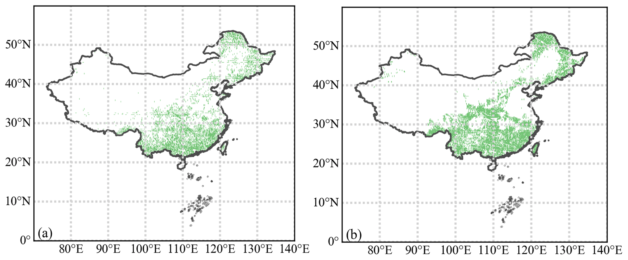
Figure A1 The distributions of the original sample pixels (at a 1 km resolution) for (a) the actual effect and (b) the two potential effects.

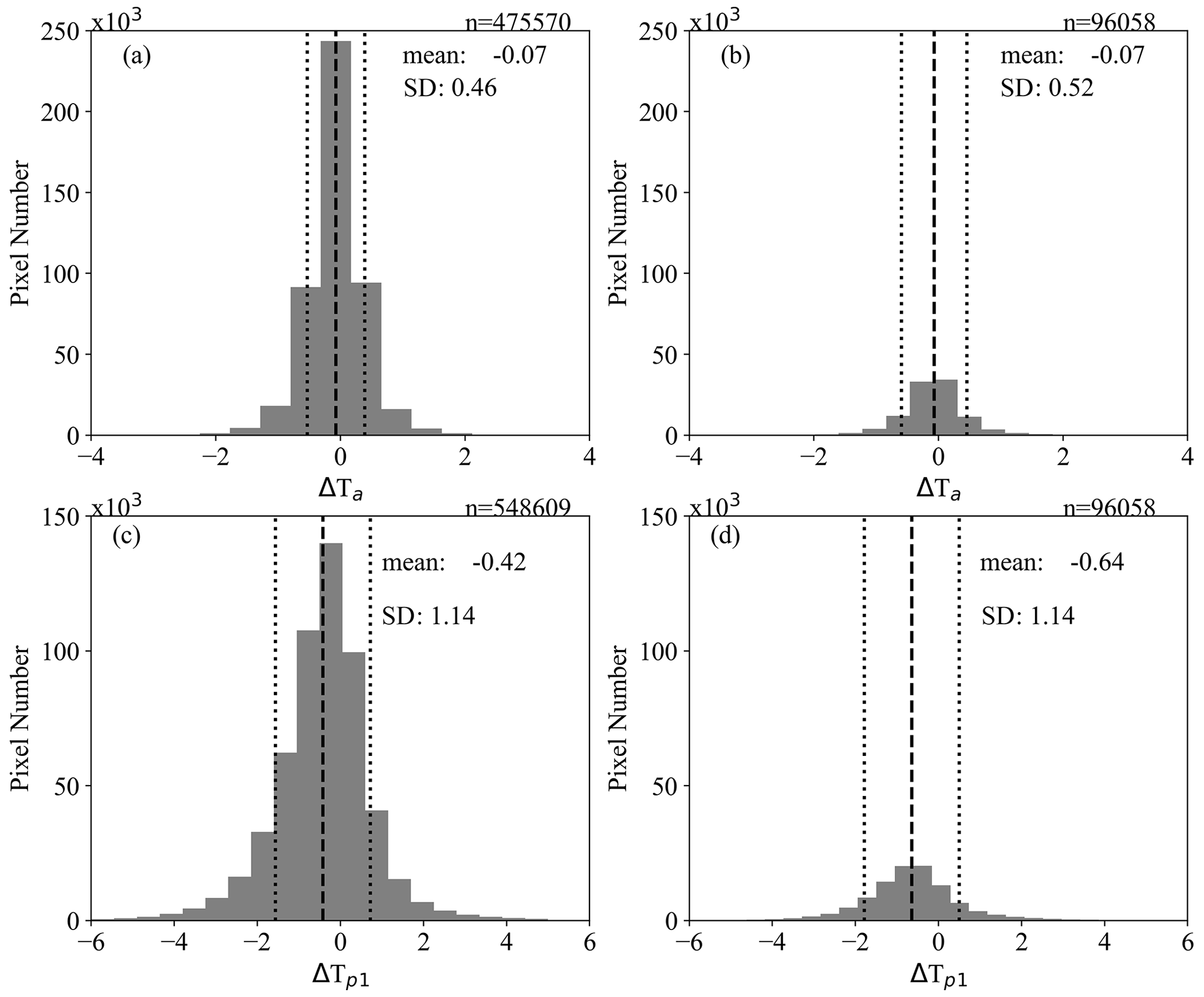
Figure A2 (a) Histogram of ΔT_a of all pixels based on the GFC dataset. (b) Histogram of ΔT_a for samples used for the statistical test. (c) Histogram of $\mathrm{\Delta }{T}_{{\mathrm{p}}_{\mathrm{1}}}$ of all pixels based on the GFC dataset. (d) Histogram of $\mathrm{\Delta }{T}_{{\mathrm{p}}_{\mathrm{1}}}$ for samples used for the statistical test.

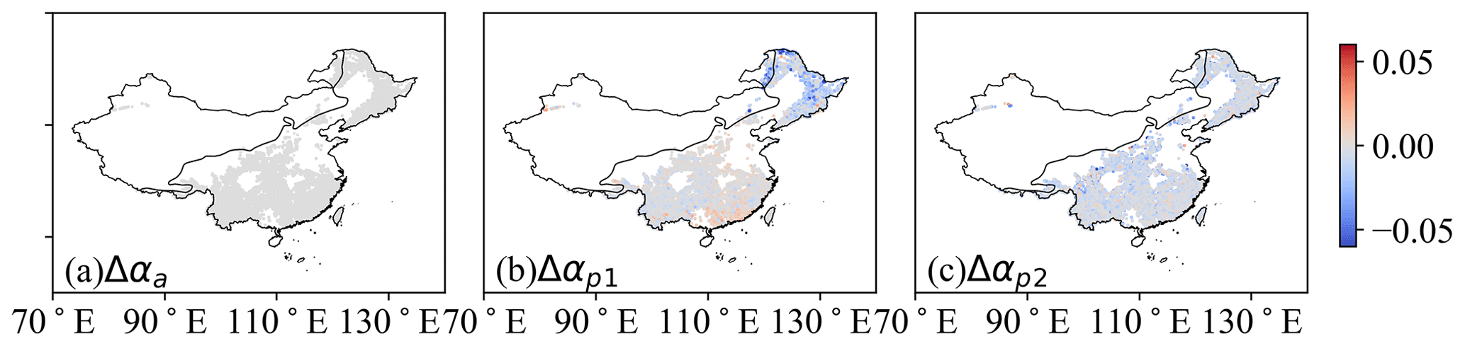
Figure A3 Spatial distribution of afforestation-induced changes in albedo (α) over China from three approaches: (a) actual albedo change following afforestation based on the space-and-time method (Δα_a), (b) mixed potential albedo change using medium-resolution land-cover maps based on the space-for-time approach ($\mathrm{\Delta }{\mathit{\alpha }}_{{\mathrm{p}}_{\mathrm{1}}}$), and (c) full potential effect ($\mathrm{\Delta }{\mathit{\alpha }}_{{\mathrm{p}}_{\mathrm{2}}}$) based on the SVD approach.

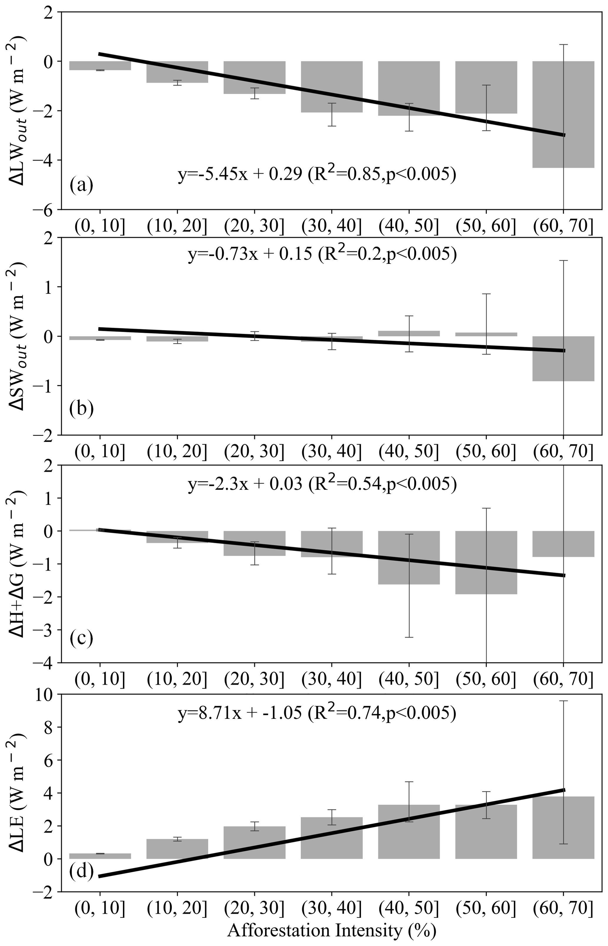
Figure A4 Changes of actual effect in (a) ΔLW, (b) ΔSW, (c) ΔH+ΔG, and (d) ΔLE (W m⁻²) as a function of afforestation intensity (F_aff) following the actual effect approach. Error bars indicate the standard error within each 10 % percent bin of F_aff. The solid black lines represent the fitted linear regression line between each energy flux variable and F_aff.

Figure A5 The mixed potential effects ($\mathrm{\Delta }{T}_{{\mathrm{p}}_{\mathrm{1}}}$) obtained based on MODIS land-cover data (MCD12Q1) and the land-cover distribution map defined at the threshold of 50 % GlobeLand30 at 1 km resolution.

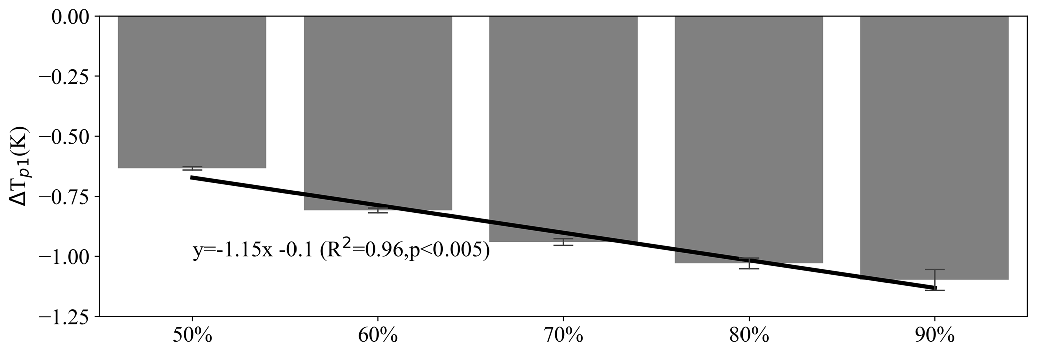
Figure A6 The influence of the forest-cover threshold applied to the land-cover map underlying the estimation of the mixed potential effect ($\mathrm{\Delta }{T}_{{\mathrm{p}}_{\mathrm{1}}}$).

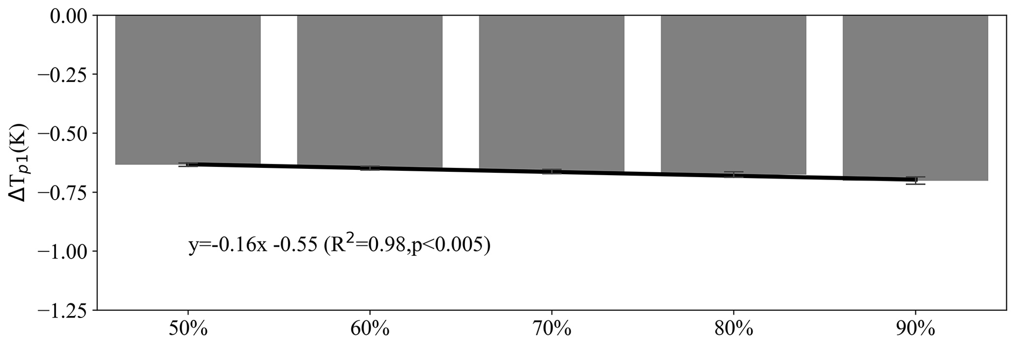
Figure A7 The influence of the openland-cover threshold used to identify a 1 km pixel as openland in the estimation of the mixed potential effect ($\mathrm{\Delta }{T}_{{\mathrm{p}}_{\mathrm{1}}}$).

Figure A8 Afforestation-induced cumulative changes in surface energy fluxes (exaJoules) in China for the period 2000–2012 following the approaches of (a) the actual effect, (b) the mixed potential effect, and (c) the full potential effect (methods in Sect. A2).

A2 Cumulative surface energy effect

The cumulative surface energy effect (f_cum) in Fig. A8 refers to the sum of the flux change (J) from all the samples while at the same time accounting for the forest change area (m²). More specifically, the cumulative surface energy change (f_cum) can be calculated from Eq. (A1):

$$\begin{array}{}\text{(A1)}& f_{\mathrm{cum}}=\sum _{i=\mathrm{1}}^{i=n}{\mathrm{area}}_i\times F_i,\end{array}$$

where F_i is the flux change per unit area (W m⁻²) for pixel i, n is the total number of samples, and area_i is the forest change area in pixel i.