Zooplankton community succession and trophic links during a mesocosm experiment in the coastal upwelling off Callao Bay (Peru)

The Humboldt Current Upwelling System (HCS) is the most productive eastern boundary upwelling system (EBUS) in terms of fishery yield on the planet. EBUSs are considered hotspots of climate change with predicted expansion of mesopelagic oxygen minimum zones (OMZs) and related changes in the frequency and intensity of upwelling of nutrient-rich, low-oxygen deep water. To increase our mechanistic understanding of how upwelling impacts plankton communities and trophic links, we investigated mesozooplankton community succession and gut fluorescence, fatty acid and elemental compositions (C, N, O, P), and stable isotope (δ¹³C, δ¹⁵N) ratios of dominant mesozooplankton and microzooplankton representatives in a mesocosm setup off Callao (Peru) after simulated upwelling with OMZ water from two different locations and different N:P signatures (moderate and extreme treatments). An oxycline between 5 and 15 m with hypoxic conditions (<50 µmol L⁻¹) below ∼10 m persisted in the mesocosms throughout the experiment. No treatment effects were determined for the measured parameters, but differences in nutrient concentrations established through OMZ water additions were only minor. Copepods and polychaete larvae dominated in terms of abundance and biomass. Development and reproduction of the dominant copepod genera Paracalanus sp., Hemicyclops sp., Acartia sp., and Oncaea sp. were hindered as evident from accumulation of adult copepodids but largely missing nauplii. Failed hatching of nauplii in the hypoxic bottom layer of the mesocosms and poor nutritional condition of copepods suggested from very low gut fluorescence and fatty acid compositions most likely explain the retarded copepod development. Correlation analysis revealed no particular trophic relations between dominant copepods and phytoplankton groups. Possibly, particulate organic matter with a relatively high C:N ratio was a major diet of copepods. C:N ratios of copepods and polychaetes ranged 4.8–5.8 and 4.2–4.3, respectively. δ¹⁵N was comparatively high (∼13 ‰–17 ‰), potentially because the injected OMZ source water was enriched in δ¹⁵N as a result of anoxic conditions. Elemental ratios of dinoflagellates deviated strongly from the Redfield ratio. We conclude that opportunistic feeding of copepods may have played an important role in the pelagic food web. Overall, projected changes in the frequency and intensity of upwelling hypoxic waters may make a huge difference for copepod reproduction and may be further enhanced by varying N:P ratios of upwelled OMZ water masses.

1 Introduction

The Humboldt Current System (HCS) is the most productive eastern boundary upwelling system (EBUS) in terms of fishery yield despite only moderate primary production rates compared with the other three major EBUSs (Bakun and Weeks, 2008; Chavez et al., 2008). About 10 % of global fish landings originate in the HCS due to wind-driven upwelling of cold nutrient-rich waters to the sunlit surface (Chavez et al., 2008). Such extraordinary high fishery yield, especially off Peru, results from a high trophic transfer efficiency compared to the other EBUSs (Chavez and Messié, 2009).

Zooplankton play the key role in transferring biomass from primary producers to pelagic fishes (Ayón et al., 2008b, 2011). Particularly, upwelling and consequent productivity dynamics are tightly coupled in the northern HCS, as indicated by the strong bottom-up-driven control of Peruvian anchovy (Engraulis ringens), the most important exploited planktivorous fish in the region. Accordingly, changes in zooplankton biomass and composition have direct consequences for higher trophic levels, e.g., fish, seabirds, and marine mammals (Ayón et al., 2008b, 2011; Aronés et al., 2019).

The HCS is characterized by a pronounced shallow and intense (acidic) oxygen minimum zone (OMZ) (Bakun and Weeks, 2008), where hypoxic waters can approach the surface (<10 m depth, Graco et al., 2017; Bach et al., 2020). Also, the HCS is characterized by massive loss and source processes of dissolved inorganic nitrogen (N) and phosphorus (P), respectively (Ingall and Jahnke, 1994; Kalvelage et al., 2011), so that water masses with N:P ratios substantially below the canonical Redfield ratio are upwelled into the surface layer (Franz et al., 2012a; Löscher et al., 2016). Such upwelled water masses have major impacts on total phytoplankton biomass (Franz et al., 2012b), community structure, and fatty acid composition (Hauss et al., 2012), with unclear consequences for consumers. The OMZ will further expand and intensify in the course of global climate change, with severe implications for biogeochemical cycles and pelagic life (Stramma et al., 2008; Schmidtko et al., 2017).

On the continental shelf, the zooplankton community in the Peruvian upwelling region is dominated by small herbivorous copepods that consume phytoplankton blooms in the freshly upwelled waters (Espinoza and Bertrand, 2014). As primary production decreases with distance from shore, the continental slope and oceanic zooplankton communities typically become dominated by euryphagous or carnivorous organisms such as large copepods, euphausiids, and gelatinous plankton (Ayón et al., 2008a). This large zooplankton, especially euphausiids, provides rich feeding grounds for Peruvian anchovy off the shelf, whereas on the shelf towards the coast, the contribution of copepods in their diet increases (Schwartzlose et al., 1999; Espinoza and Bertrand, 2008; Espinoza et al., 2009; Aronés et al., 2019).

The fertilizing effect of wind-driven upwelling of nutrient-rich waters in the HCS is subject to interannual variations due to El Niño events that weaken trade winds and increase the flow of warm water into the eastern equatorial Pacific, hindering upwelling of nutrient-rich deeper water (Karl et al., 1995; Escribano, 1998; Carr, 2001). Also, upwelling intensities of nutrient-rich waters are not directly correlated with primary and secondary production off Peru: intermediate-strength upwelling favors high zooplankton abundance and biomass, particularly in spring (October–November), while upwelling that is too strong or too weak hampers zooplankton productivity in winter and summer, respectively (Ayón et al., 2008a; Chavez and Messié, 2009; Aronés et al., 2019). Whether climate change will cause wind and hence upwelling intensities and patterns in the Pacific to decline or increase is currently not clear (Bakun and Weeks, 2008; Gruber et al., 2012), but wind and thus upwelling in the poleward portions of EBUSs have intensified, and this trend is expected to continue (García-Reyes et al., 2015).

High fish production has been attributed to pelagic fish feeding directly on phytoplankton, suggesting high trophic transfer efficiency (Ryther, 1969; Walsh, 1981). More recent studies revealed the dominance of mostly large zooplankton (copepods and euphausiids) in the diet of anchovies (Konchina, 1991; Espinoza and Bertrand, 2008, 2014) and of smaller copepods, fewer euphausiids (compared to anchovies), and potentially also some phytoplankton in the diet of Pacific sardines (Espinoza et al., 2009). Such findings emphasize the key role of zooplankton in the pelagic food web off Peru, and Espinoza and Bertrand (2008) hypothesize a more efficient use of primary production by zooplankton in the HCS than in other EBUSs, facilitating the high fish production.

Zooplankton species composition and biomass off Peru vary strongly on short timescales due to advection, peaks of larval production, trophic interactions, and community succession (Ayón et al., 2008a). Zooplankton composition itself is regulated by food quality and composition. Times of low primary production favor euryphagous or carnivorous over herbivorous zooplankton (Ayón et al., 2008a). In fact, microzooplankton and mesozooplankton seem to control phytoplankton standing stocks over the shelf (Minas et al., 1986; Cullen et al., 1992; Franz et al., 2012a).

We conducted a large-scale in situ mesocosm experiment in the coastal Peruvian upwelling region off Callao, Peru, in austral summer 2017 to investigate impacts of upwelling on pelagic biogeochemistry, plankton communities, and food web dynamics. We simulated upwelling events by adding two different types of OMZ waters with different N:P signatures to each of four mesocosms. However, bioavailable inorganic nitrogen (N) concentrations in the collected OMZ source water were lower than expected. For this reason, the N difference established through the addition of OMZ water in the mesocosm treatments with a moderate and an extreme N:P signature (2.89 and 1.49, respectively) was only minor (2.2 µmol L⁻¹) but significant directly after the additions (Bach et al., 2020). Initially, diatoms dominated the phytoplankton communities in the mesocosms. After OMZ deep-water addition and concurrent exhaustion of N, the communities shifted towards a pronounced dominance of the mixotrophic dinoflagellate Akashiwo sanguinea. Initially ranging between 1.4 and 4.9 µg L⁻¹ in the mesocosms, chlorophyll a increased only slightly after OMZ water addition to average mesocosm-specific concentrations of max. 5.6 µg L⁻¹ between day 12 and day 40 without any pronounced peak or treatment separation. Only towards the end of the experiment (after day 40) did eutrophication due to defecating seabirds (guanotrophication) lead to an intense phytoplankton bloom and concurrent increase in chlorophyll a to values around 20 µg L⁻¹ in most mesocosms.

The goal of the present work was to study the mesozooplankton (MeZP) community response to the stimulated upwelling events and to investigate trophic links in OMZ-influenced waters. Our hypotheses were as follows. (1) The efficient utilization of a phytoplankton bloom stimulated through upwelled deep waters by MeZP is higher at higher N:P stoichiometry (the moderate OMZ treatment) of upwelled water masses. To address this, we measured gut fluorescence and fatty acid compositions of dominant copepods to study whether feeding rates and contributions of biomarker fatty acids (Dalsgaard et al., 2003) increased differently at the two treatment levels. (2) The added OMZ water mass with the higher N:P stoichiometry would lead to higher zooplankton abundance and biomass compared to those with lower N:P (the extreme OMZ treatment). This was addressed by monitoring the temporal development (abundance, biomass) of the MeZP community in the mesocosms over the 50 d experiment duration. Furthermore, correlation analysis of dominant copepod species with phytoplankton simultaneously monitored by project collaborators (Bach et al., 2020; Bernales, 2023) was performed to gain insight into food web relations, and background information on the stable isotope (SI) and elemental composition (C:N) of dominant zooplankton taxa is provided. Concomitantly, we monitored the MeZP in the adjacent Pacific shelf waters at one sampling point near the mesocosm field to gain insight into the in situ zooplankton community development.

2 Methods

2.1 Experimental design

A detailed description of the mesocosm setup and the experimental manipulation is given in Bach et al. (2020). Briefly, eight KOSMOS mesocosm units (cylindrical 18.7 m long polyurethane bags, 2 m diameter, 54.4 ± 1.3 m³ volume) were deployed on 23 February 2017, close to San Lorenzo Island about 6 km off Callao (12.0555 ^∘ S, 77.2348 ^∘ W, Fig. 1). Nets (mesh size 3 mm) attached to both ends of the bags prevented larger plankton or nekton from entering the mesocosms during deployment. These meshes were removed as soon as the mesocosms were closed at the bottom with the sediment trap and the bags lifted above the surface, i.e., when the experiment started. On 25 February (defined as day 0), the mesocosms were closed at the bottom with a sediment trap. To simulate upwelling with differing inorganic N:P ratios (i.e., with an extreme and a moderate OMZ signature), water was collected on day 5 at station (hereafter St.) 1 from 30 m depth (12.03 ^∘ S; 77.22 ^∘ W) and on day 10 at St. 3 from 70 m depth (12.04 ^∘ S; 77.38 ^∘ W) of the Instituto del Mar del Perú (IMARPE) time series transect (Graco et al., 2017) using the 100 m³ deep-water collectors described by Taucher et al. (2017). In each mesocosm ∼20 m³ of water was exchanged with deep water from St. 3 (moderate OMZ signature: mesocosms M2, M3, M6, M7) or St. 1 (extreme OMZ signature: M1, M4, M5, M8). Deep water was injected on day 11 and day 12 to similar depth ranges as water had been removed from each mesocosm before (14–17 and 1–9 m).

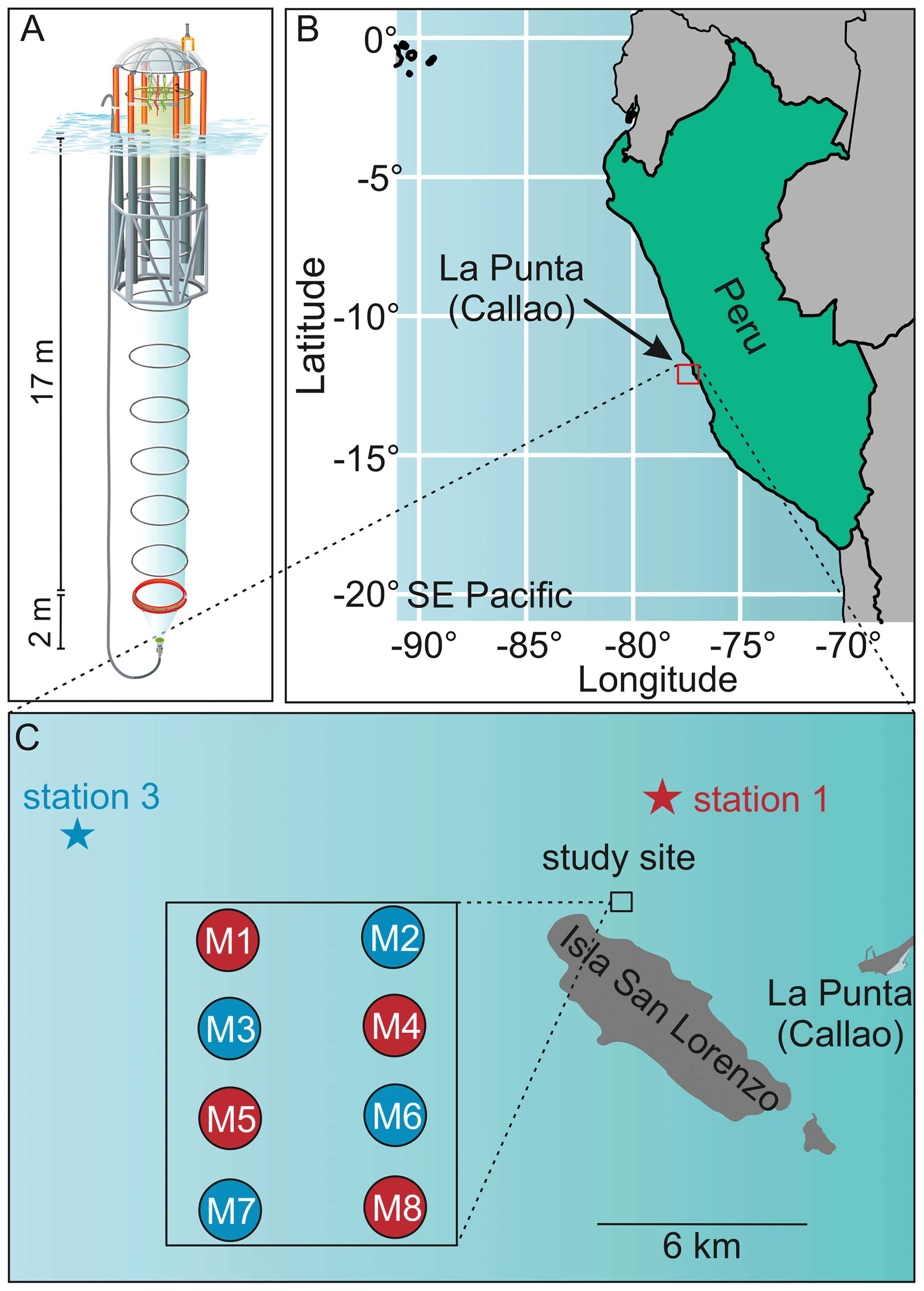
Figure 1 Study site of the mesocosm experiment. (a) One KOSMOS mesocosm unit with dimensions of the polyurethane bag and of the sediment trap. We acknowledge reprint permission of parts of this graphic from the AGU (Bach et al., 2016). (b) Location of the study region off La Punta (Callao). IMARPE and the laboratories for sample processing were located in La Punta (Callao). (c) Enlarged map of the study site that was located at the northern end of San Lorenzo Island. The additional square shows the mesocosm setup. OMZ water masses were collected at the IMARPE permanent stations 1 and 3 indicated by the stars. This figure is a reprint of Bach et al. (2020).

Oxygen minimum zones may reach very close to the surface (<10 m) in the near-coastal region off Peru (Graco et al., 2017). To conserve the low-O₂ bottom layer in the mesocosms that had established after the addition of low-oxygen deep water over the entire experimental duration, water column stratification was artificially maintained by evenly injecting a concentrated NaCl brine solution into the bottom layers of each mesocosm on day 13 and day 33. Otherwise, convective mixing induced through heat exchange with the surrounding Pacific would have destroyed the oxygen minimum layer in the mesocosms. For more details on the exact procedure of water exchange and deep-water injection as well as addition of the brine solution see Bach et al. (2020). According to these authors the mesocosm experiment was subdivided into three main phases based on the phytoplankton development: phase 1 lasted from day 1 until the OMZ water addition (day 11–12) and was characterized by a diatom-dominated phytoplankton community. Phase 2 started with the OMZ water addition until day 40 and was characterized by a bloom of the mixotrophic dinoflagellate Akashiwo sanguinea. Phase 3 continued from day 40 until the end of the experiment, when eutrophication by defecating seabirds (guanotrophication) triggered a late phytoplankton bloom in most mesocosms.

2.2 Zooplankton sampling

MeZP samples were always obtained with an Apstein net of 17 cm opening diameter equipped with a 100 µm net bag. Integrated vertical hauls were taken from 17 m depth of each mesocosm and the Pacific close to the mesocosm field. Due to technical and logistic constraints, regular sampling was not possible before day 18. Therefore, sampling intervals varied between 2 and 7 d until day 18. From then onwards, sampling was performed every 6 d. In total, two net hauls from each mesocosm and the Pacific were collected on 10 sampling days (day 0, 8, 10, 13, 18, 24, 30, 36, 42, 48). Contents from one net of each mesocosm were used for species abundance and biomass determination, and contents from the other were used for picking live organisms for fatty acid and elemental analyses (C, N, P, δ¹³C, δ¹⁵N). MeZP was sampled in the afternoon between 13:00 and 17:00 (local time). As soon as the abundance net haul was retrieved onboard, the zooplankton sample was emptied into sample bottles with filtered seawater (100 µm), and the net and cod end were subsequently rinsed to also wash zooplankton attached to the mesh into the sample bottle. The second net for live organisms was carefully poured into 5 L sampling containers prefilled with 4 L of filtered seawater at ambient temperature to accommodate zooplankton organisms and reduce stress. All net samples were stored in cooling boxes to prevent heating until returning to the laboratory and further processing.

Microzooplankton samples for elemental composition analysis (detailed in Sect. 2.8) were collected from integrated water samplers (see detailed description of water samplers in Bach et al., 2020). In total, samples were taken on 12 sampling days (day 0, 8, 10, 13, 16, 18, 20, 26, 30, 36, 42, 48) from each mesocosm and the Pacific. On the first sampling day 0, samples were collected from the depth intervals 5–0 and 17–5 m. From day 8 onwards, sampling depths were 10–0 and 17–10 m. Until day 20, samples were regularly taken from both sampling depth intervals; after day 20 only the upper interval (10–0 m) was sampled for microzooplankton because concentrations in the deeper layer were too low to reach detection limits.

2.3 Abundance and species determinations

In the laboratory, the net samples taken for abundance and biomass determination of each mesocosm were split in half (Motoda splitter), and one-half of each sample was preserved in 4 % formaldehyde–seawater solution for subsequent microscopic species identification and enumeration. The other half was used for ZooScan analyses. The formalin-preserved abundance subsample was split by applying the Huntsman Marine Laboratory (HML) beaker technique, producing count results with a coefficient of variation of 9 %–15 % from the effective mean (van Guelpen et al., 1982). Subsequently, aliquots were counted under a stereomicroscope (Nikon SMZ 1270) until at least 50 individuals of the most abundant taxa were counted; rare species and taxa were counted from the whole sample. As usual, zooplankton abundances were calculated assuming 100 % filtering efficiency of the net. However, variation among samples is normally high due to plankton patchiness, and moreover variation is species- and taxon-specific (Wiebe and Holland, 1968).

2.4 ZooScan

For the scanning procedure, samples were split further (Motoda splitter) to ratios between 1:4 and 1:32 to avoid crowding in the scanning chamber. In the laboratory, samples were scanned on an Epson Perfection V750 Pro scanner in a modification of the ZooScan method (Gorsky et al., 2010) and a scan chamber constructed of a 21 by 29.7 cm (DIN A4) glass plate with a plastic frame. Scans were 8-bit greyscale, 2400 DPI images (tagged image file format; *.tif). The scan area was partitioned into two halves (i.e., two images per scanned frame) to reduce the size of the individual images and facilitate the processing by ZooProcess/ImageJ. “Vignettes” and image characteristics of all objects were extracted with ZooProcess (Gorsky et al., 2010) and sorted sequentially by first clustering and naming using MorphoCluster (Schröder et al., 2020) and then predicting the remaining unsorted images using deep-learning features in Ecotaxa (http://ecotaxa.obs-vlfr.fr/ (last access: 25 May 2021), Picheral et al., 2017). Automated image sorting was manually validated by experts. Individual biomass was derived from the image area of each object using published taxon-specific relationships (Lehette and Hernández-León, 2009).

2.5 Zooplankton grazing, gut fluorescence

Grazing rates of the dominant copepods Paracalanus sp. were analyzed with the gut fluorescence (GF) method (Mackas and Bohrer, 1976) via experimental determination of gut clearance rates (clearance coefficient). Clearance rate determination assumes that maximum gut fullness of organisms equals initial gut pigment in the gut clearance experiment (time point 0 min, T_0 min). The experimental identification of a clearance coefficient is accomplished through fluorescence determination of organisms' guts allowed for clearance over a series of time steps for a total period of ca. 1 h. At least eight time steps along the time axis are recommended. Hence, pre-determination of in situ daily maximum gut fullness is required if maximum ingestion rates are to be estimated (Båmstedt et al., 2000).

Copepods often have diel feeding rhythms (Mackas and Bohrer, 1976). Therefore, prior to clearance rate determination of mesocosm copepods, the feeding rhythmicity and time of maximum gut fullness of dominant copepods (Paracalanus sp.) were examined twice over a 24 h cycle for copepods collected in both the adjacent Pacific and in the mesocosms. Each time zooplankton net samples were taken, adult female copepods (the dominant copepodite stage) were picked and GF measured (see below for more details on the procedure). These investigations proved that copepods' feeding activities, i.e., times of maximum gut fullness, were highest at night between approximately 22:55 and 03:40 (Fig. 2). Therefore, sampling of zooplankton in the mesocosms for clearance rate determinations was done at night on occasions: during the night of day 21–22 and during the night of day 34–35. MeZP samples were collected in all mesocosms with the same Apstein net of 17 cm opening diameter as mentioned above but equipped with a 200 µm net bag and a non-filtering cod end to collect organisms gently and prevent stress evacuation of their guts before retrieval of the net.

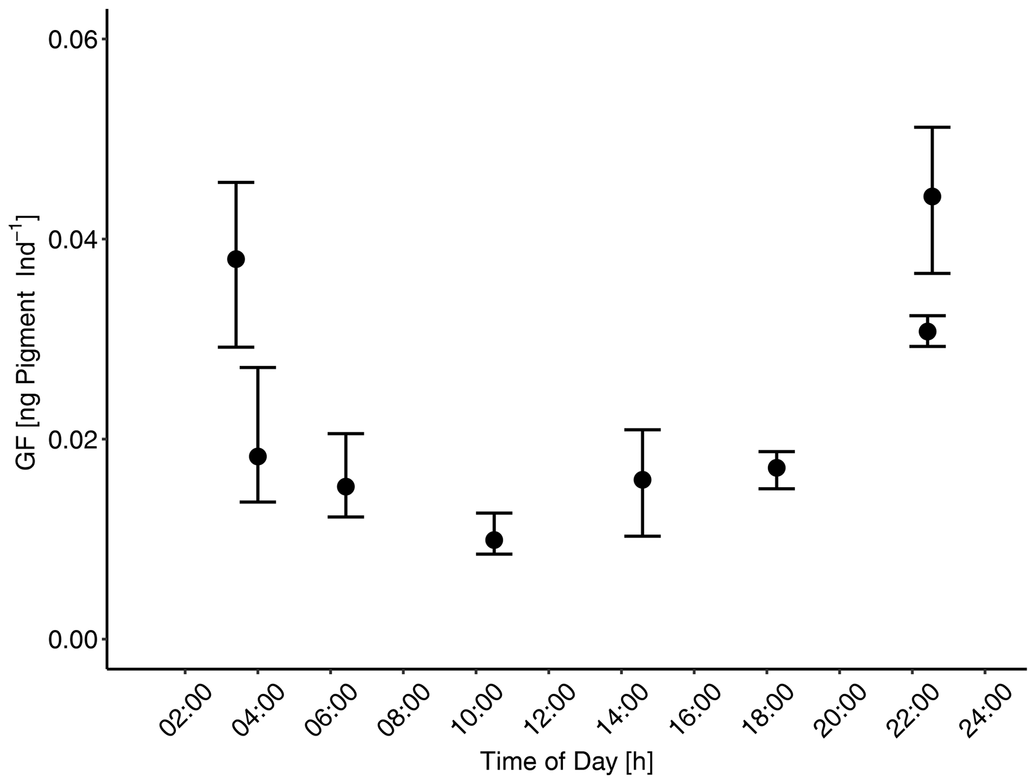
Figure 2 Gut fluorescence [ng pigment Ind⁻¹]: diel feeding rhythm to determine time of maximum gut fullness of adult female Paracalanus sp. Gut fluorescence was analyzed on females collected over a 24 h cycle in the mesocosms. Maximum gut fullness was detected early in the morning (03:44) and 1 h before midnight (22:55). Error bars depict 95 % confidence intervals.

Determination of gut clearance rates and coefficients followed recommendations by Båmstedt et al. (2000). Immediately after retrieval of each net haul, the zooplankton sample was split into eight subsamples. One of the subsamples was immediately concentrated over a 200 µm mesh; the mesh was carefully folded not to squash organisms, wrapped in aluminum foil, and immediately shock-frozen in liquid nitrogen to preserve the in situ state of gut content upon catch (time point 0 min, T_0 min). The other seven subsamples (T_8 min–T_56 min) were each incubated in 500 mL of filtered seawater (20 µm) to allow copepods to evacuate their guts. After each 8 min, one of the incubated subsamples was terminated (i.e., last sample after 56 min, T_56 min) by concentrating the zooplankton on a 200 µm mesh; the mesh was wrapped in aluminum foil and immediately shock-frozen in liquid nitrogen. The shock-frozen subsamples (T_0 min–T_56 min) were stored at −80 ^∘C until further processing in the home laboratories in Kiel.

Paracalanus (mostly Paracalanus parvus) was the dominant copepod taxon in all mesocosms and was therefore chosen for determination of gut clearance rate. In Kiel, depending on availability, between 8 and 52 individual adult female Paracalanus sp. were picked on crushed ice under a stereomicroscope (Wild Heerbrugg M3) from each of the frozen subsamples (T_0 min–T_56 min) into 2 mL cryovials placed in a labtop vial cooler at −15 ^∘C. This procedure was done under dimmed room light, usually within half an hour to prevent destruction of fluorescent pigments (Båmstedt et al., 2000). Loaded vials were stored at −80 ^∘C until completion of all samples from all mesocosms. Subsequently, gut pigments were extracted in 1.2 mL 90 % acetone with the help of glass beads (0.5 mm diameter) in a Precellys Evolution HP homogenizer at 10 000 RPM (9168 g) for 15 s. Constant cooling of samples was ensured during the whole procedure to avoid pigment degradation. After 30 s of pause, the crushed samples were treated in a Sigma 3–18 K centrifuge for 10 min at 10 000 RPM (9168 g) at 4 ^∘C to separate the liquid and solid phase. Finally, the liquid phase was filtered through 0.2 µm PTFE filters to remove any remaining solid body parts. GF was then measured with a Trilogy Laboratory Fluorometer (Turner Design, USA). The relative GF of each sample was measured three consecutive times and converted to absolute values (ng pigment µg DM⁻¹) by means of a chlorophyll standard curve. To eliminate background fluorescence caused by astaxanthin carotenoids in copepod tissues, GF was corrected by GF measured for female Paracalanus collected in the surrounding Pacific and starved for 24 h to allow animals to empty their guts completely (Mackas and Bohrer, 1976). An exemplary sample was analyzed for gut pigments (or their degradation products) also by means of reverse-phase high-performance liquid chromatography (HPLC, Barlow et al., 1997) calibrated with commercial standards.

To normalize GF, dry mass (DM) of female Paracalanus individuals was determined for each time-point subsample. Single female copepods were picked for DM determination of each sample in triplicate (i.e., three samples with one female from each mesocosm if enough organisms were available). Organisms picked for DM determination were rinsed in Milli-Q and transferred into pre-weighed tin cups before drying at 60 ^∘C for 24 h and mass determinations on a Mettler Toledo XP2U Ultra Micro Balance (accuracy: 0.000058–0.0034 µg). Additionally, females from day 21–22 samples were picked for C:N determinations, usually from T_0 min and T_56 min (13–38 individuals per sample depending on availability). Carbon and nitrogen elemental analyses were done on a Euro EA – CHNSO element analyzer according to Sharp (1974).

2.6 Fatty acid analysis of dominant copepods

Adult females (the dominant developmental stage) of the dominant copepods Paracalanus sp. and Hemicyclops sp. were picked as soon as possible after collection for lipid analysis from the second net (for live organisms). Due to time constraints, female copepods were only picked from six mesocosms (M2, M3, M6 of the moderate treatment; M1, M4, M5 of the extreme treatment). Lipid samples of female copepods from the adjacent Pacific could only be picked during phase 3 because of limited abundance during phases 1 and 2. If available, up to 80 individuals (minimal 16) of each species were sorted to ensure sufficient lipid mass above detection limit. Some samples were directly transferred to dichloromethane : methanol (2:1, $v/v$) in 8 mL analytical vials equipped with Teflon-sealed screw caps, and some were transferred to Eppendorf caps without solvent. The latter allowed for determination of DM after lyophilization. DM of specimens directly stored in dichloromethane : methanol (2:1, $v/v$) could not be determined. Samples were stored at −80 ^∘C until further analysis in the home laboratory at Bremen University.

DM of the copepods was determined after lyophilization for 48 h (CHRIST Alpha). Total lipids were extracted from the samples after Folch et al. (1957) and Hagen (2000) with dichloromethane : methanol (2:1 $v/v$). For quantification of total fatty acids (TFA), tricosanoic acid (23:0) was added as an internal standard prior to extraction and TFAs were expressed as the percentage of fatty acids in relation to the DM of the sample (TFA % DM). For Paracalanus, TFAs were related to the mesocosm-specific mean DM of females used for gut fluorescence determination because DM determined after lyophilization of lipid samples was inaccurate. Lipid extraction of samples stored in solvent followed the same procedure as for the lyophilized samples.

Fatty acids were converted to their methylester derivatives (FAME) by transesterification for 4 h at 80 ^∘C in hexane and methanol containing 3 % concentrated sulfuric acid (Kattner and Fricke, 1986). FAMEs were extracted with aqua bidest and hexane and analyzed by gas chromatography (Agilent Technologies, GC model 7890A). The device was equipped with a DB-FFAP column (30 m length, 0.25 mm inner diameter) and a programmable temperature vaporizer injector, operating with helium as a carrier gas (Peters et al., 2007). Fatty acid and alcohol components were detected using a flame ionization detector (FID) and identified by their retention times in comparison to known fatty acid and alcohol standard compositions (FAMEs and free alcohols of the copepod Calanus hyperboreus and Supelco 37 Component FAME Mix). In some cases, the lipid mass was very low with a stronger impact of impurities so that gas chromatography did not result in reliable data. Therefore, data presented here are those that have at least 70 % purity of fatty acids relative to impurities. The fatty acid compositions were evaluated according to the fatty acid trophic marker (FATM) concept of Dalsgaard et al. (2003).

2.7 Elemental composition (C, N, O, P) and stable isotope (δ¹³C, δ¹⁵N) signatures of mesozooplankton

Bulk samples of copepods or polychaetes were used for the analysis of stable isotope signatures (δ¹³C and δ¹⁵N) and carbon (C), nitrogen (N), and particulate organic phosphorus (POP) content. Copepod samples mainly contained the taxa Paracalanus sp. and Hemicyclops sp., whereas polychaetes were separated into the species Paraprionospio sp. and Pelagobia longicirrata. Copepods and polychaetes were pipetted through a 55 µm nylon mesh attached to a polypropylene tube of ∼2 cm length so that the organisms remained on the mesh. Organisms were shortly rinsed with Milli-Q water. Bulk samples were transferred to pre-weighed tin capsules (5×9 mm, Hekatech) and dried at 60 ^∘C for at least 24 h. After drying, tin capsules were closed at the top and stored in a 96-well plate covered with Parafilm. In the home laboratories, samples were dried again and weighed on a microbalance. Subsamples for phosphorus were taken whenever enough biomass of the sample was available. Target sample masses were 1–4 mg for C:N and 1–10 mg for POP. Stable isotopes (¹³C and ¹⁵N) as well as C and N contents were analyzed at the UC Davis Stable Isotope Facility using a PDZ Europa ANCA-GSL elemental analyzer interfaced to a PDZ Europa 20–20 isotope ratio mass spectrometer (Sercon Ltd., Cheshire, UK) with helium as a carrier gas. Vienna Pee Dee Belemnite and atmospheric air were used as standards to determine the carbon and nitrogen ratio, respectively. Stable isotope ratios are reported with reference to a standard and expressed in parts per thousand (‰) according to the formula ${\mathit{\delta }}^{\text{H}}X=\left[\right(R_{\text{SAMPLE}}/R_{\text{STANDARD}}$)], where X is the respective element, H gives the heavy isotope mass of that element, and R is the ratio of the heavy to the light isotope.

POP was determined photometrically on a Hitachi U-2900 spectrophotometer as orthophosphate after oxidative decomposition by adding spatula-tip Oxisolv^®, 5 mL of Milli-Q, and the sample to Pyrex tubes and autoclaving. After cooling to room temperature, a subsample (dilution 1:5 or 1:10) was measured according to Ehrhardt and Koeve (1999).

2.8 Elemental composition (C, N, P) of microzooplankton

Samples for X-ray microanalysis (XRMA) were prepared following Segura-Noguera et al. (2012). 500 mL water samples were taken from each mesocosm and the Pacific Ocean and were pre-filtered through a 200 µm nylon mesh to remove larger MeZP. The 200 µm filtered water samples were further concentrated via inverse filtration (vacuum pump, 15 µm nylon mesh) to a volume of approximately 2–4 mL. These 2–4 mL remaining water samples were pipetted through a 15 µm nylon mesh so that the organisms remained on the mesh, where they were rinsed several times with ice-cooled Milli-Q brought to pH of 8.3–8.5 with NaOH. The last ∼50 µL was pipetted to a slide (in several drops) and checked under a stereomicroscope for microzooplankton organisms. 5 µL was transferred to a transmission electron microscopy (TEM) grid (coated with a formvar carbon film on copper on 75 mesh, Agar Scientific) in triplicate and again shortly checked under the stereomicroscope to ensure that there was a sufficient number of organisms from the same species to be analyzed. TEM grids were air-dried for about 1 h and afterwards transferred to TEM grid storage boxes and stored in a desiccator container (Fisherbrand™ Circular Bottom Desi-Vac™ container, Fisher Scientific) until arriving in the home laboratories in Germany. Samples were then kept in vacuum bags until final analysis.

XRMA was done at the Joseph Banks Laboratories in Lincoln, UK. Single cells of microzooplankton (200–20 µm) were imaged and analyzed for C, N, O, and P elemental content in an FEI Inspect scanning electron microscope (SEM) equipped with an energy-dispersive spectrometer Oxford X-Act silicon drift detector (SDD). X-ray spectra were acquired from an area that circumscribes the cell at 20 kV of accelerating voltage, accumulation time of 120 s (lifetime), spot size 6.0, and 10 mm working distance. Following the analysis of each cell, a blank spectrum (i.e., formvar only) close to the cell was acquired for 30 s lifetime. Spectra from cells that drifted, changed shape, or charged during analysis were discarded. An image before and after the analysis was taken using the INCA Oxford EDS software, and the area of analysis was calculated with a MATLAB routine. X-ray bremsstrahlung from each spectrum was removed using NIST DTSA-II Jupiter 6 November 2017, and the intensity of each peak was also calculated with a MATLAB routine. The standards used for quantification were latex beads of 3 and 5 µm for C and ADP for N, O, and P. Latex beads of 3 µm were analyzed as internal standards several times during each analysis session to correct for drift and for changes in day-to-day beam intensity. A detailed description of the measuring approach is given in Segura-Noguera et al. (2016).

2.9 Data evaluation, statistical analysis

We applied repeated measures ANOVA (rmANOVA) to test for possible treatment effects. Response variables (listed in Table 1) were modeled as a function of deep-water treatment (two levels: “moderate” and “extreme”) and experiment day with mesocosm as a random factor to test for significant differences between the added deep waters with different OMZ signature. Normality and variance homogeneity of residuals were tested graphically. In the case of significant results, if assumptions were not met, data were log₁₀-transformed and re-analyzed. Unfortunately, ∼50 % of the fatty acid samples showed a substantial level of impurities due to the generally very low lipid content of the copepods and were therefore omitted from the data set; i.e., only samples with at least 70 % purity are included in the present study. This led to a restricted data set with unbalanced sampling design and an unequal and low number of replicates that did not allow for more comprehensive statistics (rmANOVA). Instead, we calculated mean percentages and their 95 % confidence interval (CI) of the dominant fatty acids per mesocosm treatment and experimental phase to allow for basic statistical inference. Comparing any two means, evidence of significance can be inferred if their CIs do not overlap (Field et al., 2012). Similarly, initial GF values of copepods of each mesocosm (with standard deviation, SD) are shown together with treatment means and their 95 % CIs because measured GF in the copepods' guts of both OMZ treatments was too low to allow for grazing rate estimations.

Pearson correlations between abundance of the dominant zooplankton taxa, the copepods Paracalanus sp. and Hemicyclops sp., and counts of dominant phytoplankton and microzooplankton groups (diatoms, phytoflagellates, coccolithophores, dinoflagellates, silicoflagellates, ciliates, all in cells L⁻¹) as well as with concentrations of extracted phytoplankton pigments (Chloro-, Dino-, Crypto-, Prymnesio-, and Pelagophyceae, diatoms, Synechococcus, all in µg L⁻¹) and with total chlorophyll a (µg L⁻¹) were performed to gain insight into food web relations.

All statistics were performed using R 4.2.2 (libraries emmeans, lme4, lmerTest, and HighstatLib.V6; R Core Team, 2014).

3 Results

3.1 Zooplankton abundance and contribution of taxonomic groups

Average total abundance of MeZP was very similar at the start of the experiment, and no significant differences developed between the two OMZ deep-water treatments over the course of the experiment (Table 1). However, the established treatment differences with respect to N:P signatures were significant but only small. Thus, any potential small-scale treatment differences in MeZP abundance, if existent at all, would have most likely been hidden by methodical uncertainties associated with net sampling, patchy distribution, and counting bias (Algueró-Muñiz et al., 2017; Lischka et al., 2017).

Variability of the manual counts of total MeZP abundance (individuals per liter: Ind L⁻¹) was high between mesocosms and sampling days. Average total MeZP abundance varied between 6.3 Ind L⁻¹ (CI 3.5) on day 30 and 52.7 Ind L⁻¹ (CI 14.0) on day 42 in the moderate-treatment mesocosms and between 7.2 Ind L⁻¹ (CI 3.3) on day 30 and 33.9 Ind L⁻¹ (CI 30.1) on day 42 in the mesocosms with the extreme treatment. Total abundance of MeZP sampled in the adjacent Pacific station was in a similar range as numbers estimated in the mesocosm treatments (9.7–129.3 Ind L⁻¹) and peaked on day 48 (Fig. 3). Individual mesocosms developed some more distinct abundance peaks at the beginning and towards the end of the study with maximum numbers of 112.3 Ind L⁻¹ in M1 on day 10, 127.9 Ind L⁻¹ in M4 on day 42, and 129.0 Ind L⁻¹ in M3 on day 48. Deep-water additions on day 11 and day 12 after removal of approximately 20 m³ of water from each of the mesocosms, respectively (Bach et al., 2020), resulted in distinct deviation from average MeZP abundance between day 13 and day 18 with temporarily higher numbers in the moderate mesocosms. This deviation was only short-term, not significant, and due to some higher abundance in M7 (moderate treatment), causing the relatively large confidence intervals (Table 1, Fig. S1 in the Supplement). It had equalized by day 24 but was indicative of different MeZP densities of the two injected deep-water masses.

Table 1 Results of repeated measures ANOVAs. OMZ treatments (levels: moderate, extreme) and experiment day (T_day = day 13–day 48) served as independent variables (FACTOR). Abundance and biomass of zooplankton categories and stable isotope content of copepods served as dependent variables and are listed below as RESPONSE. Mesocosm was used as a random effect in the linear models. Response variables that were log₁₀-transformed are indicated (log₁₀). Alpha level for p=0.05. Note that single effects of the experiment day (time) are not listed as they are not of interest in the present study but were for most response variables significant (p<0.05). df: degrees of freedom.

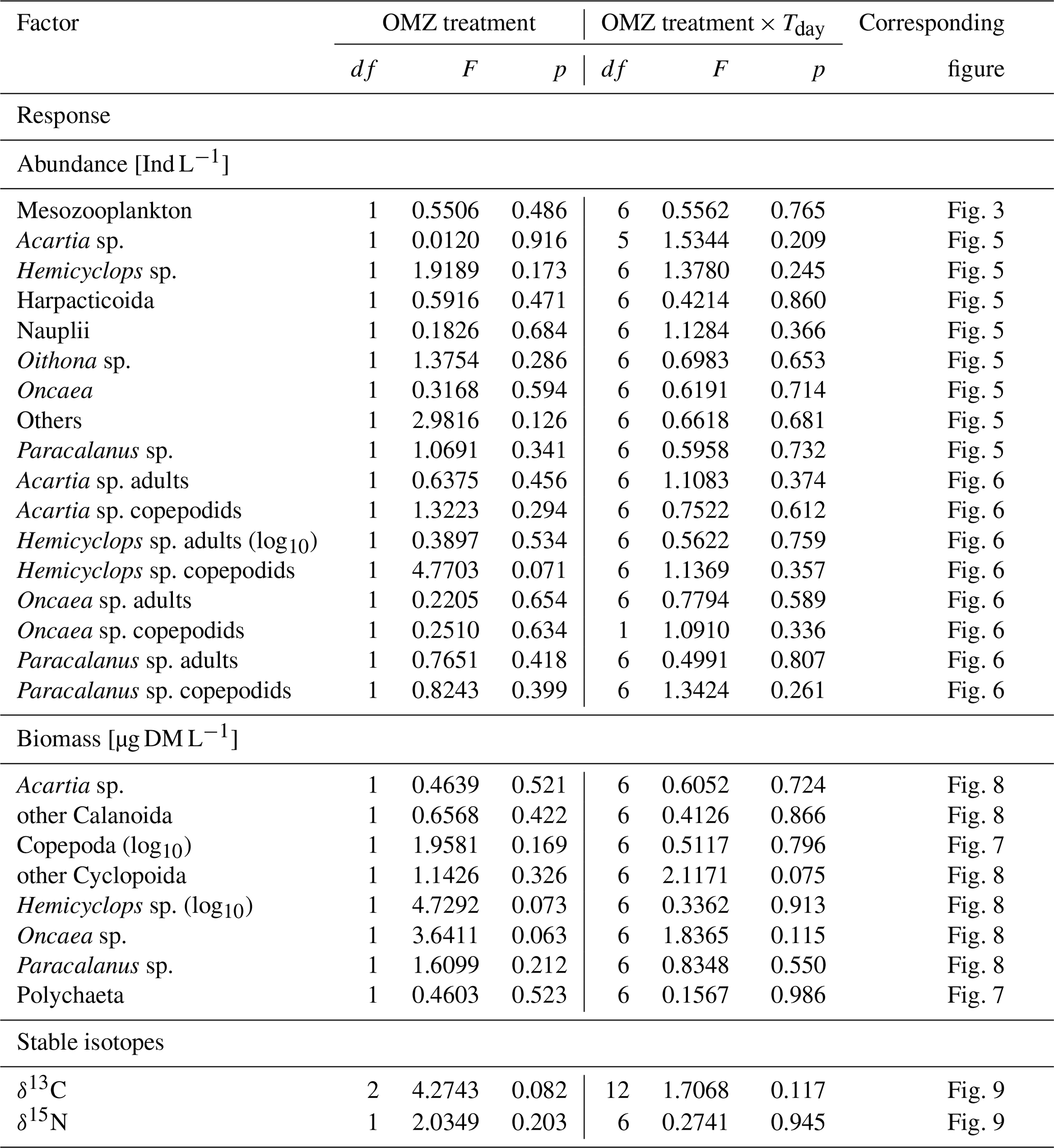
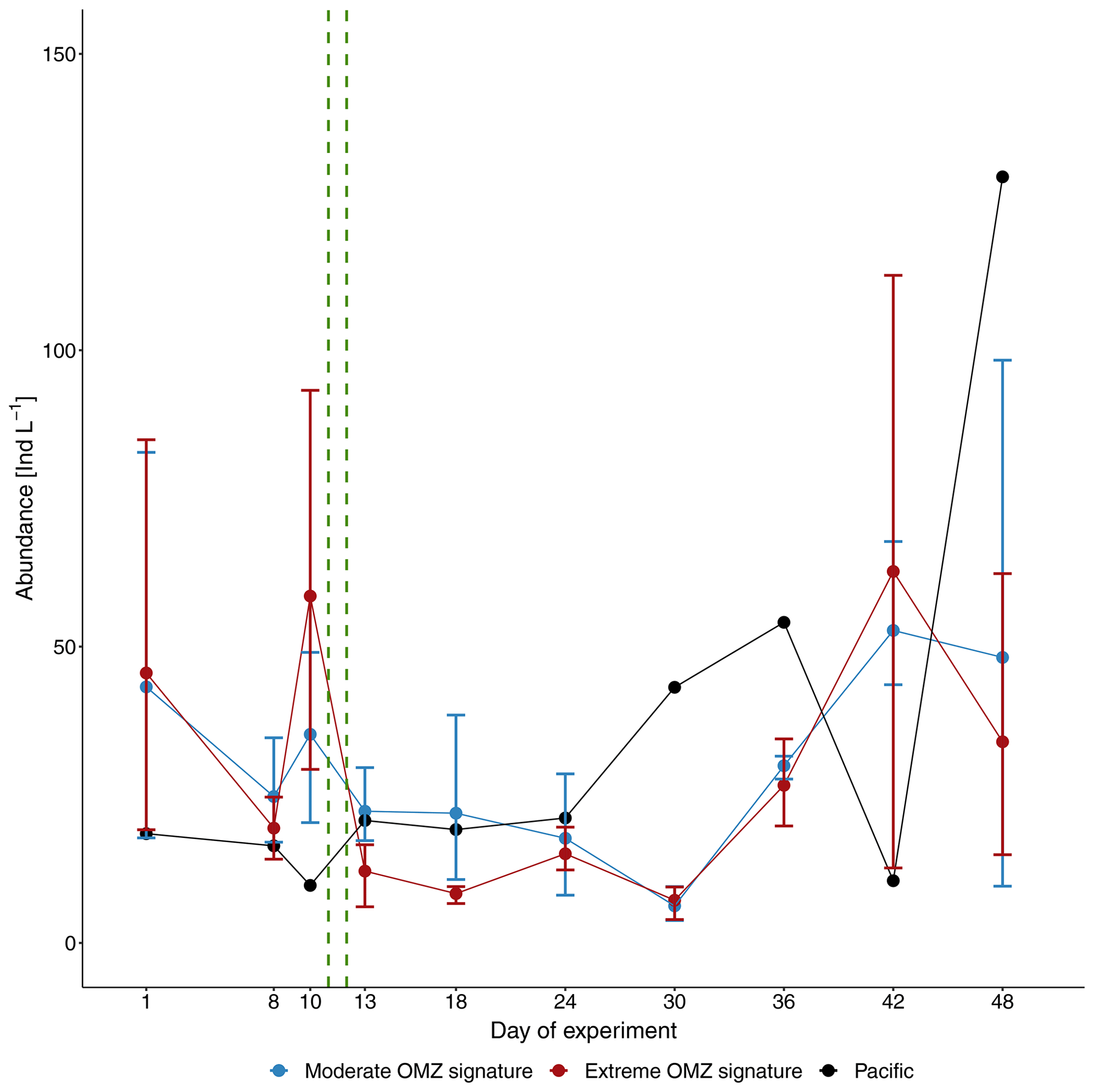
Figure 3 Average total abundance of mesozooplankton (individuals per liter, Ind L⁻¹) in the mesocosms with moderate and extreme OMZ signatures and the adjacent Pacific station. Error bars depict 95 % confidence intervals. The green vertical dashed lines indicate the days of OMZ water additions.

In terms of abundance, copepods dominated the zooplankton communities at all times both in the mesocosms and the adjacent Pacific. Other taxa (in descending order of contribution: Polychaeta, Echinodermata, Euphausiacea, Mollusca, Hemichordata, Cnidaria, Chordata, Cirripedia, Rotifera) contributed only between 0.2 % and 18 %. Higher shares of other taxa were found only until day 18, and afterwards they were negligible. This pattern essentially reflected the occurrence of copepods and other taxa in the surrounding Pacific (0.3 %–24 %), although in the Pacific other taxa contributed higher shares to the zooplankton community compared to the values found in the mesocosms also after day 18 (Fig. 4a).

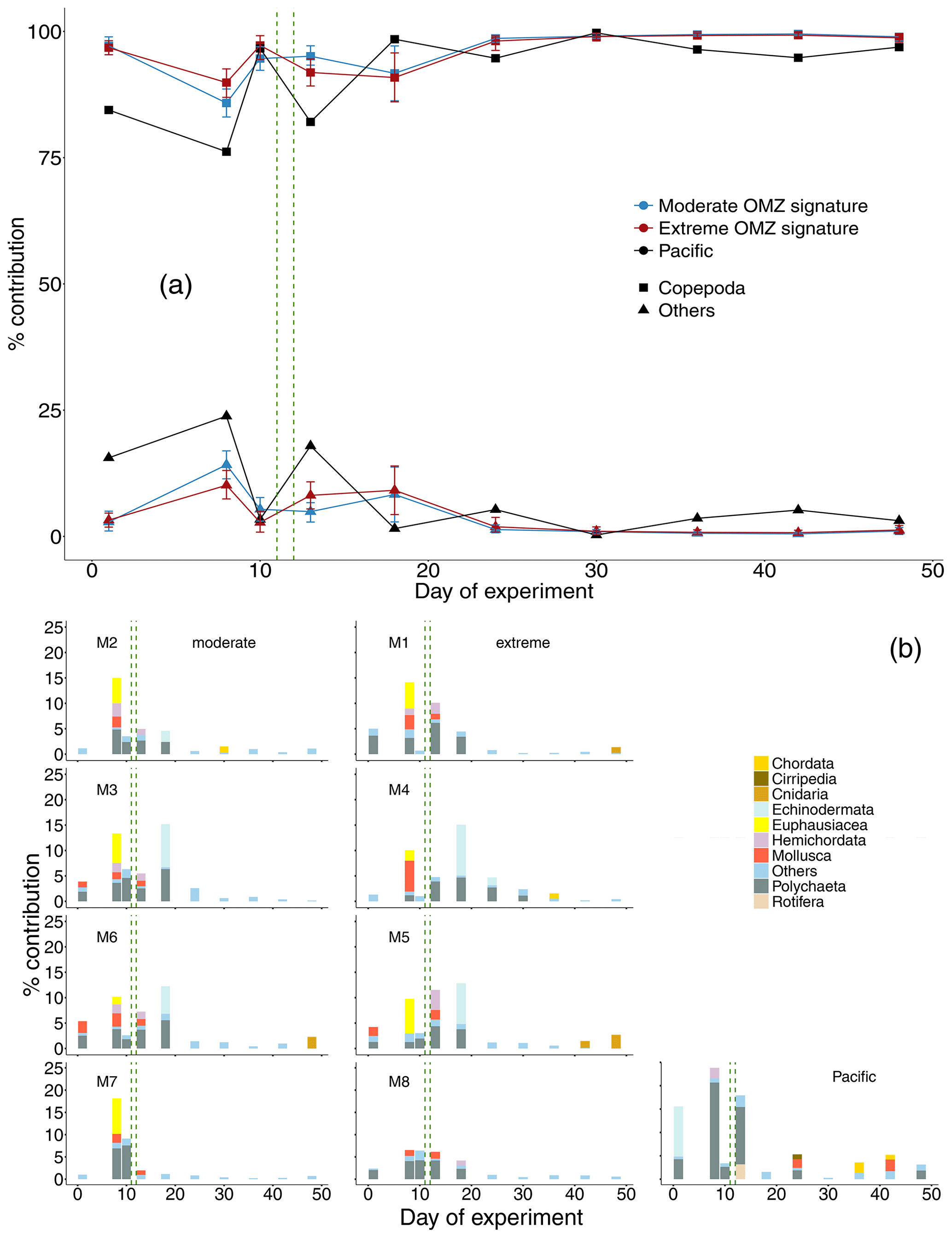
Figure 4 (a) Percent contribution of major taxonomic groups to total mesozooplankton abundance: Copepoda and “others” (Chordata, Cirripedia, Cnidaria, Echinodermata, Euphausiacea, Hemichordata, Mollusca, Polychaeta, Rotifera). Shown is the mean across OMZ treatments (moderate and extreme signature mesocosms, respectively) with 95 % confidence intervals and the contribution of copepods and “others” in the Pacific. (b) The percent contribution of the category “others” as shown in (a) split into taxonomic groups. The category “others” summarizes all taxonomic groups that contributed less than 1 % on a particular sampling day. The green vertical dashed lines indicate the days of OMZ water additions.

Among other taxa, in the mesocosms, Polychaeta, Echinodermata, Euphausiacea, and Mollusca (taxa ordered in decreasing trend) were most abundant, sometimes constituting more than 5 % of total abundance. Remaining taxa consistently contributed less than 5 % to total MeZP abundance. Towards the end of the study, the numbers of Chordata (ichthyoplankton) and Cnidaria increased in M1, M2, M4, M5, and M6 to values >1 %. In the Pacific in the early phase of the experiment, Polychaeta (up to 21 %) and Echinodermata (up to 11 %) dominated, followed by Hemichordata (2 %) and Rotifera (3 %). In the second half of the experiment, Polychaeta, Cirripedia, Mollusca, and Chordata (each <3 %) dominated the generally low share of other taxa in total abundance. Chordata (ichthyoplankton) increased because fish eggs were added to the mesocosms on day 31; however, they did not stay for long in the mesocosms (Bach et al., 2020) (Fig. 4b).

3.1.1 Dominant copepods

The enclosed copepod community was dominated by Hemicyclops sp. at the time of mesocosm closure. Hemicyclops sp. continued to dominate in the moderate treatment almost throughout the experiment (up to 65 % on day 36), whereas in the mesocosms of the extreme treatment, after the deep-water addition Paracalanus sp. increased to similar percent contributions as Hemicyclops (up to 54 % on day 18 and up to 60 % on day 13, respectively) (Fig. 5). The genus Paracalanus comprised two different species, P. parvus and P. cf. quasimodo. P. parvus was numerically dominant and occurred with all copepodite stages. P. cf. quasimodo was found only in the adult stage. The variability of the percentage share over time of Hemicyclops sp. and Paracalanus sp. in the surrounding waters of the Pacific was higher than observed in the mesocosms.

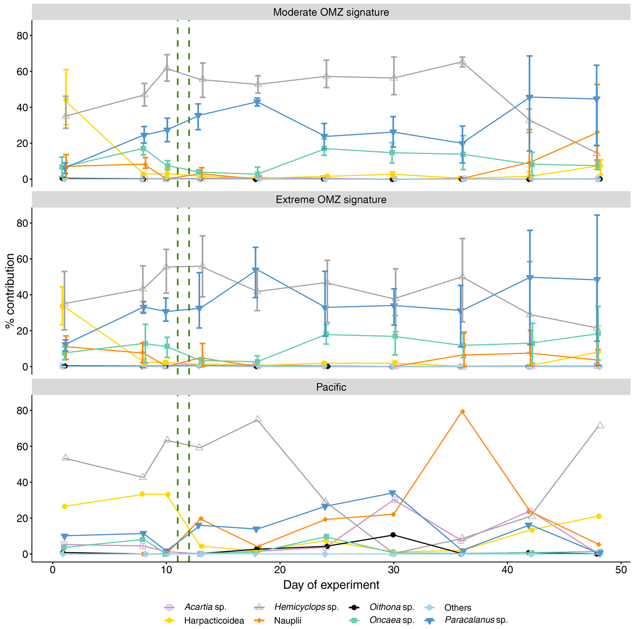
Figure 5 Percent contribution of copepod genera and copepod nauplii to total copepod abundance. Shown is the mean across OMZ treatments (moderate and extreme signature mesocosms, respectively) with 95 % confidence intervals and the contribution of each category in the Pacific. The category “others” comprises copepods of the genera Calanus, Centropages, Clausocalanus, Corycaeus, Clytemnestra, Eucalanus, Euterpina, Labidocera, Mecynocera, Microsetella, Scolecithrix, and Temora. The green vertical dashed lines indicate the days of OMZ water additions.

Acartia sp., usually the dominant neritic species in these coastal upwelling areas, was consistently low in both mesocosm treatments (up to 1 % mean portions), whereas it ranged 0.1 %–30 % in the adjacent Pacific. Five different species of the cyclopoid genus Oncaea were registered: Oncaea venusta, O. cf. chiquito, and three other Oncaea species that could not be identified to species level. Especially in the second half of the experiment, Oncaea sp. was the third most abundant copepod genus in both treatments. The cyclopoid genus Oithona occurred with four different species: O. nana, O. cf. nana, and two undetermined Oithona species. Oithona sp. had consistently low abundances in the mesocosms (<1 %) but contributed 10.6 % on day 30 in the adjacent Pacific.

Harpacticoid copepods occurred in the mesocosms at the beginning but decreased quickly after the start of the experiment in both treatments (≤8 %). The succession of harpacticoid copepods in the surrounding Pacific was more variable than in the mesocosms (8 %–33 %). Opposite to the adjacent Pacific, the occurrence of copepod nauplii in the mesocosms was low during most of the experiment in both treatments. In the moderate treatment, nauplii contributed between 9.4 % and 0 % over time. Only towards the end of the experiment did nauplii increase to 26.2 %. In the extreme-treatment mesocosms nauplii contribution varied between 14.8% and 3.6 %. Nauplii contribution in the surrounding Pacific was almost consistently higher than in the mesocosms (up to 79 %).

Copepods of the category “others” comprised the genera Calanus, Centropages, Clausocalanus, Corycaeus, Clytemnestra, Eucalanus, Euterpina, Labidocera, Mecynocera, Microsetella, Scolecithrix, and Temora. This category accounted on average for less than 1 % of total copepod abundance in all mesocosms as well as the Pacific during the whole experiment duration.

For none of these species or groups were significant effects between the mesocosm deep-water treatments determined (Table 1).

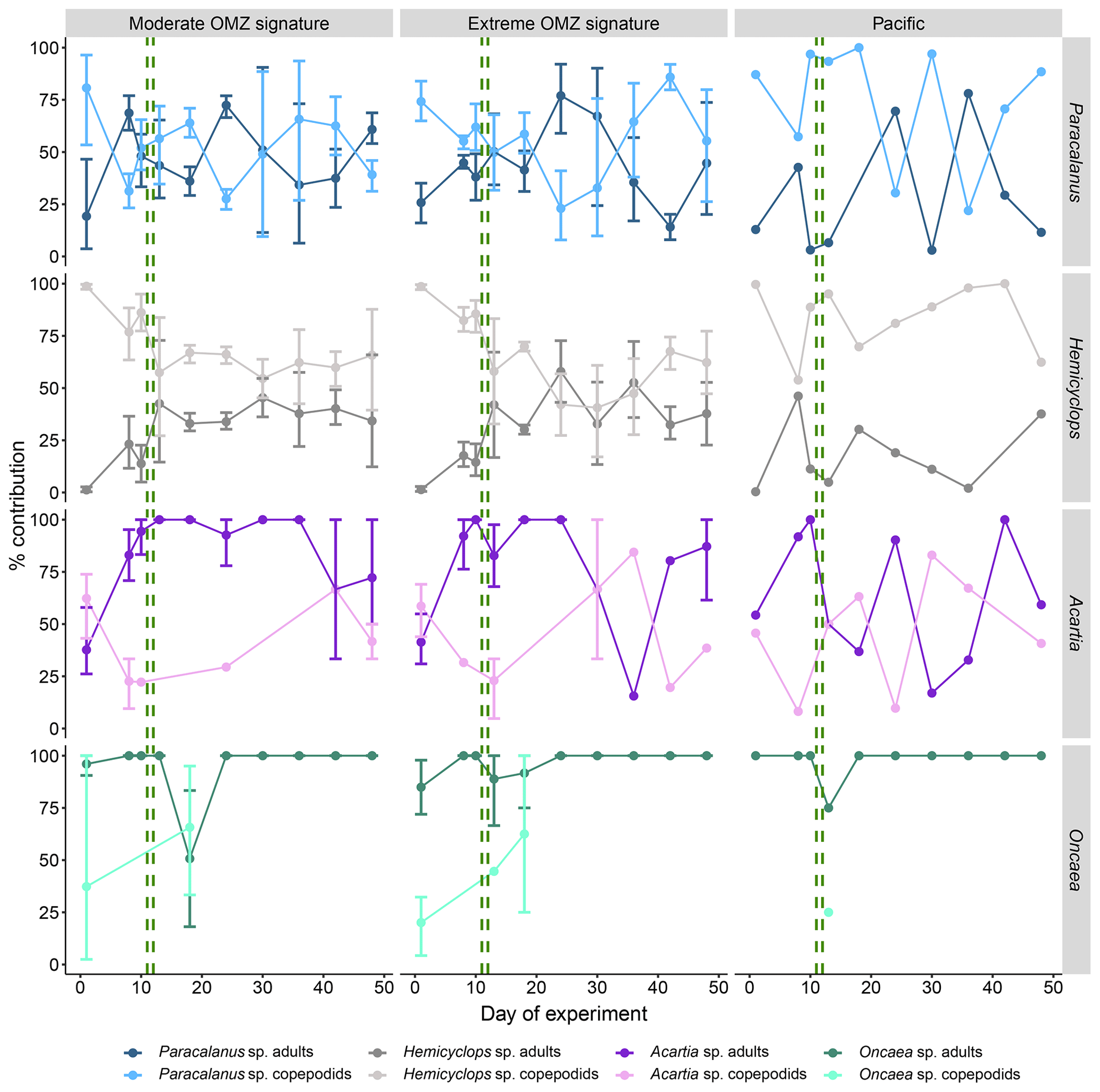
Figure 6 Temporal succession of developmental stages of dominant copepods (average percent contribution to total genus abundance with 95 % confidence intervals). Adults comprise female and male copepods, and copepodids comprise stages CI–CV. The green vertical dashed lines indicate the days of OMZ water additions.

3.1.2 Succession of developmental stages of dominant copepods

Overall, succession patterns of developmental stages of the different copepod species in the mesocosms did not vary significantly between the deep-water treatments. In the case of Paracalanus sp. and Hemicyclops sp. copepodids usually outnumbered adults in both mesocosm treatments (Fig. 6); only sporadically did adults account for more than 60 %–70 %. The stage contribution of Paracalanus in the Pacific was mostly in favor of copepodids (usually >50 %), except for day 24 and day 36 with >70 % adult copepods. The portion of Hemicyclops copepodids in the surrounding Pacific was consistently higher throughout the experiment and always higher than 50 %. Acartia sp. copepodids dominated in both mesocosm treatments at the experiment start. Thereafter, the population matured and consisted predominantly of adult copepods. The stage distribution of Acartia sp. in the surrounding Pacific was more variable. Oncaea sp. almost exclusively occurred in the adult stage in both the mesocosms and the Pacific.

3.2 Zooplankton biomass

For the dominant taxa, the ZooScan method reduced the systematic variability and added the size information for each object, allowing biomass estimation. For rare taxa, manual enumeration is to be preferred because of the low split ratios in the scans.

Zooplankton biomass (as estimated based upon scanned area of individuals) was dominated by copepods (Fig. 7a), which in the mesocosms ranged between 11.8 and 75.6 µg DM L⁻¹ in the first phase, increased to between 8.58 and 137.9 µg DM L⁻¹ in the second phase, and declined again to between 4.8 and 40.8 µg DM L⁻¹ in the third phase. The second most important contributor to zooplankton biomass were polychaetes (Fig. 7b), which in the mesocosms were hardly detected on day 1 and ranged between 0 and 39.0 µg DM L⁻¹ in the first phase, between 0 and 74.7 µg DM L⁻¹ in the second phase, and between 0 and 0.65 µg DM L⁻¹ in the third phase. The highest biomass values were observed for both total copepods and polychaetes in mesocosms M2 and M3 (both in the moderate mesocosm treatment). The main contributors to copepod biomass were Paracalanus sp. and Hemicyclops sp. Due to the high variability between mesocosms, however, this treatment effect was insignificant (Table 1). In the adjacent Pacific, total copepod and polychaete biomass tended to be lower than in the experimental mesocosms but followed a similar temporal pattern (peaking in phase 2). Among the copepods, the numerically dominant genera Paracalanus and Hemicyclops were also the main biomass contributors (Fig. 8a and b), with roughly equal share and peaking in phase 2, in particular in the moderate OMZ signature treatment. Acartia, which was only present in lower abundance and biomass (Fig. 8c), tended to reach higher biomass in the extreme OMZ signature treatment (in particular in M4). Oncaea and other or unidentified cyclopoids (Fig. 8d, f) were mainly present in phase 1, with the lowest values in phase 2 and a slight increase in phase 3.

In contrast to MeZP abundance, biomass (copepods) peaked between day 10 and day 20, but the highest abundance values were found towards the end of the experiment when biomass was at a minimum. This discrepancy is most likely due to a shift in the abundance–biomass relationship of dominating zooplankton organisms towards smaller-sized or lower-mass individuals, respectively.

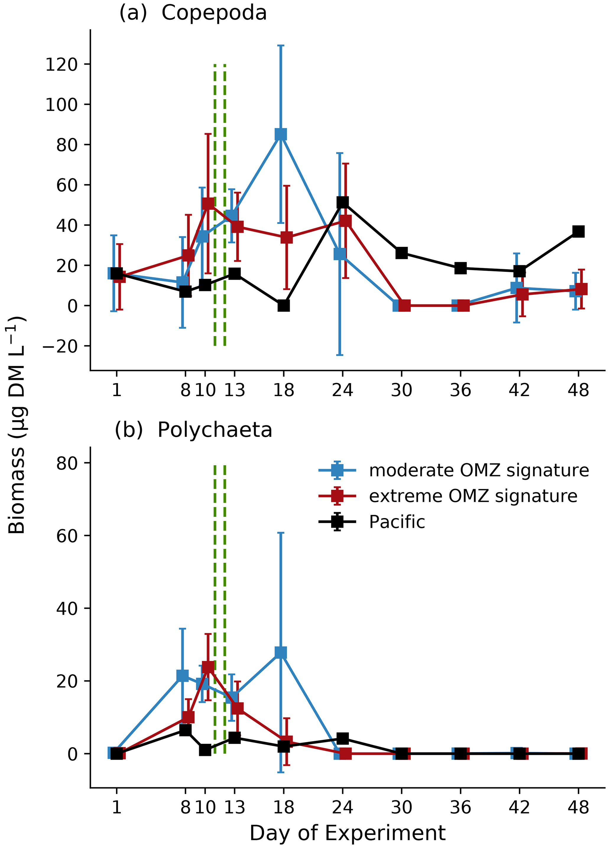
Figure 7 Biomass development (µg DM L⁻¹) averaged for the moderate and extreme treatments over time of total copepods (a) and polychaetes (b) based on image analysis (ZooScan). Blue: moderate OMZ signature, red: extreme OMZ signature, black: Pacific. Error bars depict 95 % confidence intervals. The green vertical dashed lines indicate the days of OMZ water additions. The experimental phase 1 lasted from day 1 until day 11–12, phase 2 until day 40, and phase 3 until experiment termination. Note the different y-axis scale.

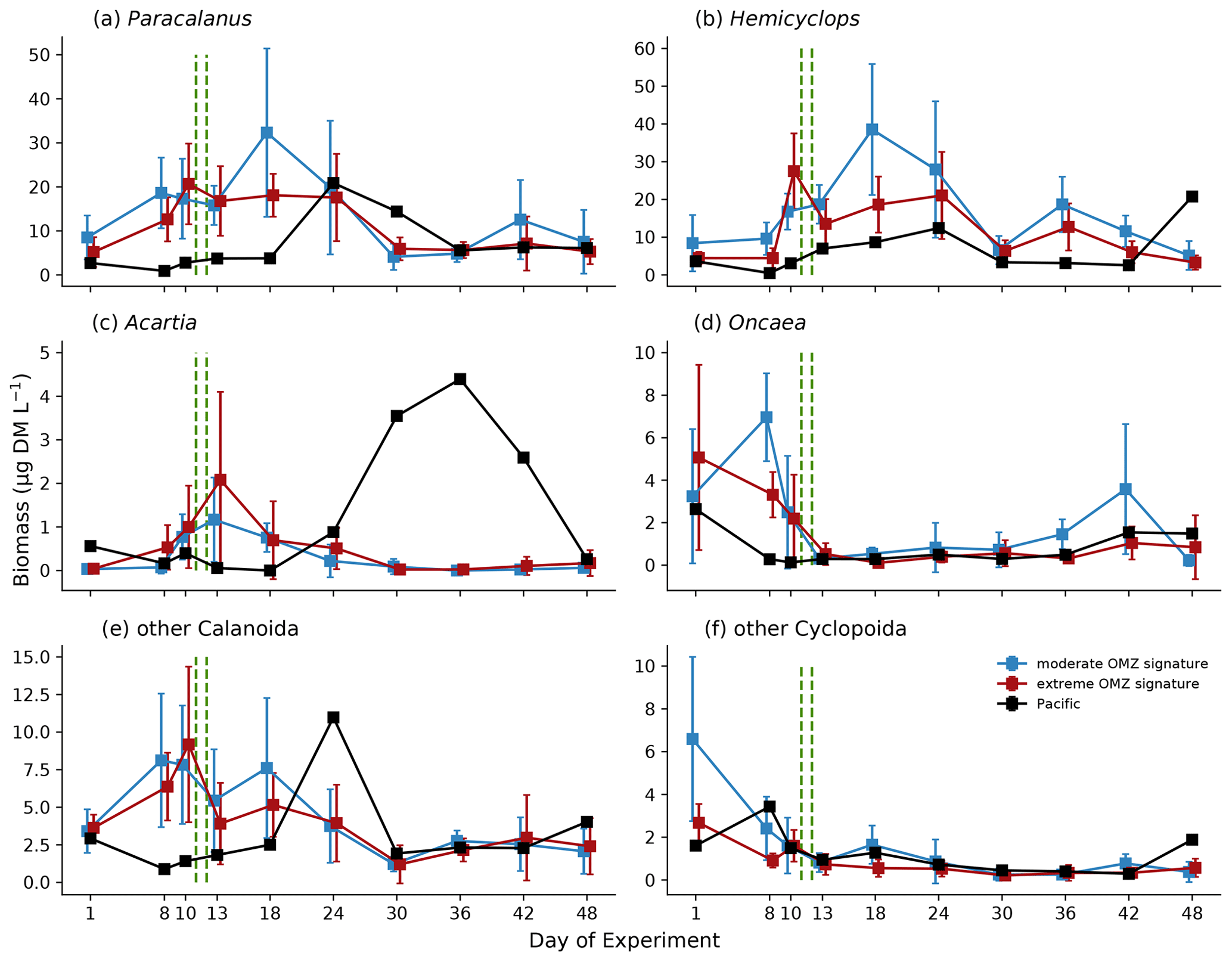
Figure 8 Biomass (µg DM L⁻¹) development averaged for the moderate and extreme treatments of major taxonomic groups during the course of the experiment. Error bars depict 95 % confidence intervals. The green vertical dashed lines indicate the days of OMZ water additions. The experimental phase 1 lasted from day 1 until day 11–12, phase 2 until day 40, and phase 3 until experiment termination. Note the different y-axis scale.

3.3 Zooplankton grazing, gut fluorescence

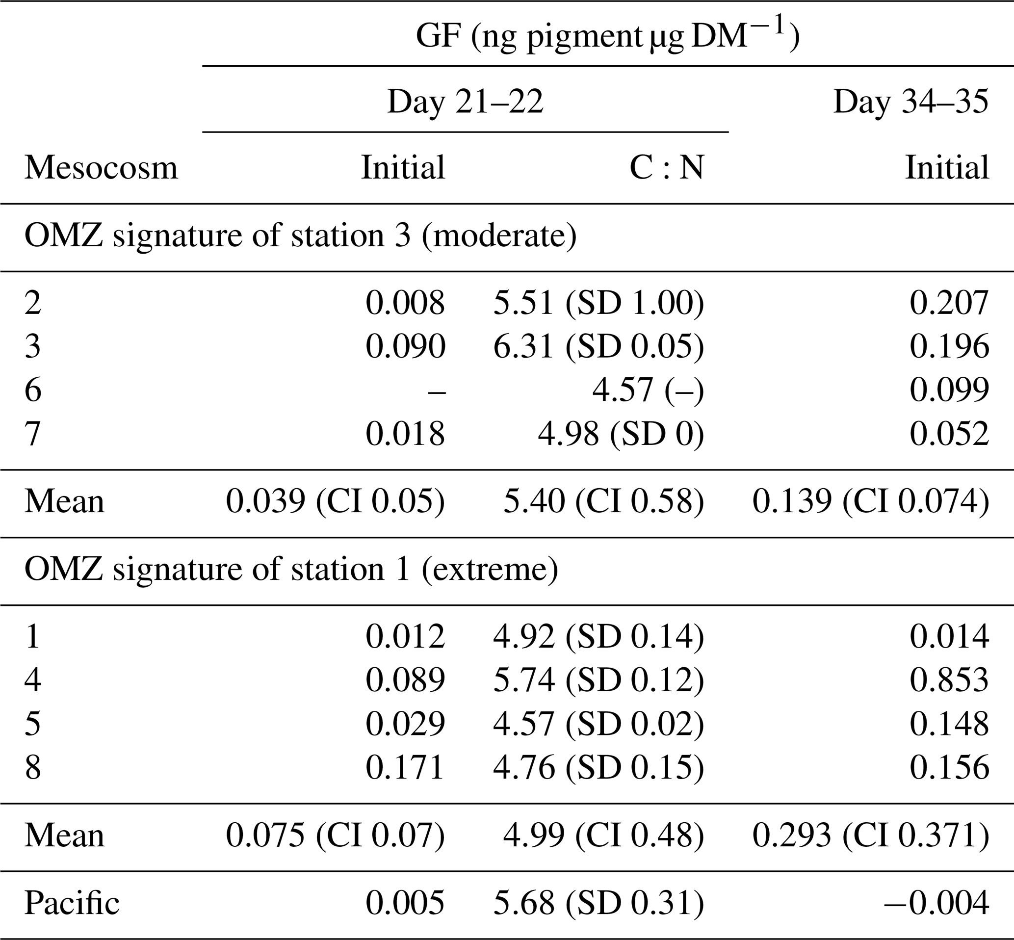
In general, initial (T_0 min) GF of Paracalanus sp. females was very low, but averages for the moderate and the extreme treatment, respectively, on day 34–35 (0.14 and 0.29 ng pigment µg DM⁻¹) were higher than on day 21–22 (0.03 and 0.08 ng pigment µg DM⁻¹), indicating somewhat higher feeding activities of Paracalanus females on autotrophic food particles later in the experiment (Table 2). Due to such low GF, no clearance rate measurements could be inferred because GF of incubated copepods showed no clear decreasing trend in GF over time (data published at PANGAEA, https://doi.org/10.1594/PANGAEA.947833, Lischka et al. (2022).) Female Paracalanus of the adjacent Pacific had even lower fluorescence in their guts (0.005 and −0.004 ng pigment µg DM⁻¹) than measured in mesocosm organisms.

Table 2 Gut fluorescence (GF, ng pigment µg DM⁻¹) of Paracalanus females collected during the night of 18–19 March 2017 (day 21–22) and during the night of 31 March to 1 April 2017 (day 34–35), immediately frozen after net retrieval on board to preserve in situ GF (initial gut fluorescence, i.e., T_0 min). Standard deviation (SD), 95 % confidence intervals (CI), and C:N values are only available for day 21–22 and are given as mol mol⁻¹.

An attempt to analyze gut fluorescence with HPLC to identify degradation products (pheopigments) of chlorophyll a and draw conclusions on potential food sources (Welschmeyer, 1994) revealed no identifiable peak(s) besides astaxanthin, which is indicative of the copepods' carapax, supporting very low GF and thus very low feeding on autotrophic food particles.

Mean C:N values for copepods in mesocosms treated with St. 3 (extreme) and St. 1 (moderate) OMZ water were 5.40 and 4.99, respectively, and had overlapping CIs; thus, no significant differences are suggested. Availability of female Paracalanus during day 34–35 was not sufficient to reach the detection limit for C:N analysis.

3.4 Lipids

Fatty acid (FA) analyses revealed a relatively high degree of impurities of the samples. This is a common problem in small copepods with rather low total lipid mass close to the detection limit (Lischka and Hagen, 2007). For this reason, identification of FA peaks in the gas chromatogram was sometimes difficult or even impossible. Therefore, data presented here only include results of samples for which at least 70 % of all peaks of a chromatogram could be identified and assigned to a specific FA (i.e., 70 % purity).

3.4.1 Total fatty acids

Total fatty acid content (TFA in % DM, equivalent to total lipid levels) of Paracalanus sp. (females) from the mesocosms was low (1.5 % DM–4.2 % DM) throughout the study period and did not vary significantly between the phases and treatments as indicated by overlapping CIs (Table 3). Mean TFAs of individuals collected in the adjacent Pacific during phase 2 fall within the range of TFA levels determined for the mesocosm copepods. Only one copepod sample from the Pacific could be analyzed in phase 3 when TFAs contributed 0.5 % to DM.

Table 3 Fatty acid compositions (% TFA) of females of Paracalanus sp. and Hemicyclops sp. (mean contributions (%) and 95 % confidence intervals – CIs) per treatment and phase of dominant fatty acids as well as the percentage of saturated (SFA), polyunsaturated (PUFA) fatty acids, and free fatty alcohols (FAlc). Data are only presented for samples for which the contribution of FAs in relation to impurities was at least 70 %. Of those, only FAs are listed, where the phase mean was ≥2 % during at least one occasion. Note that for Paracalanus TFAs were related to mesocosm-specific average dry mass (DM) of weighed females collected for gut fluorescence; in the case of Hemicyclops DM could be determined after lyophilization of copepod samples for lipid analysis and was subsequently used for calculation of percent TFA. Phase 1: day 1 to OMZ water addition (day 11–12), phase 2: starting with the OMZ water addition until day 40, phase 3: day 40 until experiment termination.

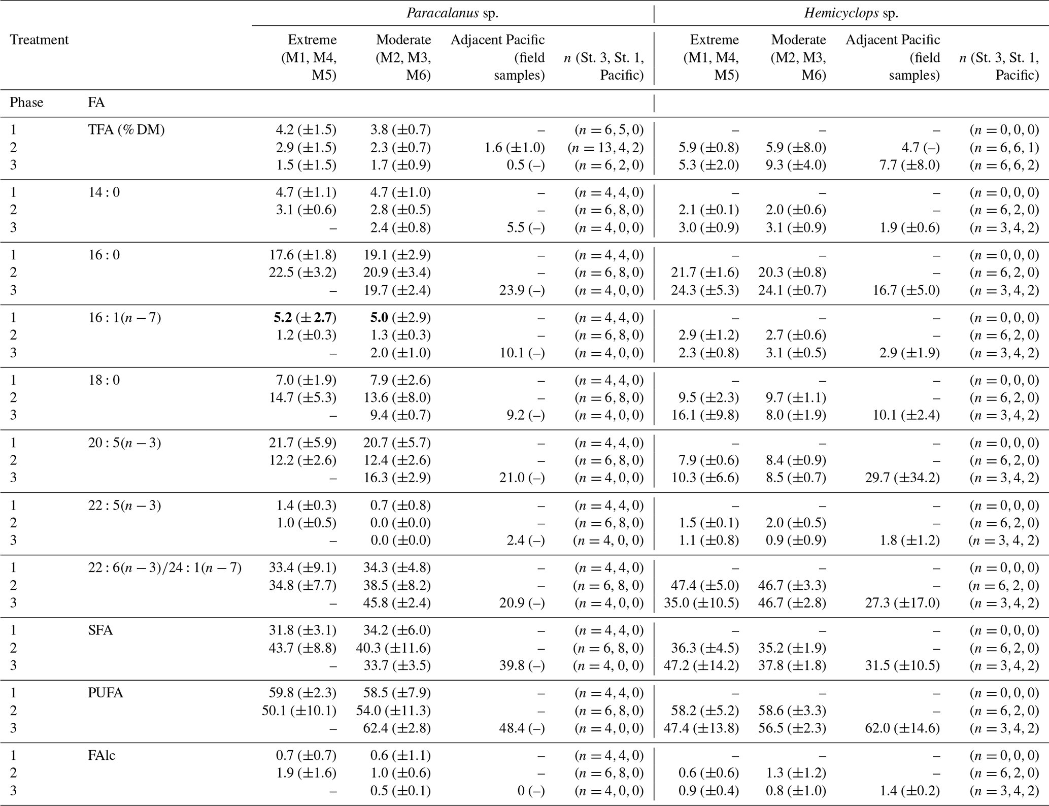
Bold values indicate values that are significantly different regarding the phase 1 value compared to phases 2 and 3.

During phase 1, Hemicyclops sp. was not numerous enough for TFA determination, but sufficient numbers of organisms were available for lipid analyses during phase 2 and 3. In these two phases, TFA levels of Hemicyclops sp. in both treatments ranged between 5.3 % DM and 9.3 % DM. During phase 3 in the moderate treatment, mean TFA levels were comparatively high (9.3 % DM), but CIs suggest no significant differences between treatments and phases. The TFA level of female Hemicyclops sp. collected in the Pacific was comparable with the mesocosm treatments during both phases.

3.4.2 Fatty acid and fatty alcohol composition

The fatty acid (FA) and fatty alcohol (FAlc) composition is presented as the mean contribution per experimental phase and OMZ treatment of specific FAs and FAlcs to total FAs and FAlcs of Paracalanus and Hemicyclops together with their CIs (Table 3). Only FAs that reached mean contributions of 2 % during at least one of the three phases and the sum of FAlcs were included in the list. Generally, mean FA and FAlc compositions of both species did not differ much over time and treatment as suggested by overlapping CIs.

Dominant FAs in Paracalanus females were $\mathrm{20}:\mathrm{5}(n-\mathrm{3})$ and $\mathrm{22}:\mathrm{6}(n-\mathrm{3})/\mathrm{24}:\mathrm{1}(n-\mathrm{7})$, typical biomembrane components. Unfortunately, the peaks of the FAs 22:6 and 24:1 overlapped in the gas chromatogram and could not be separated in all cases, although a dominance of the ubiquitous $\mathrm{22}:\mathrm{6}(n-\mathrm{3})$ can be assumed. The mean percentage of $\mathrm{20}:\mathrm{5}(n-\mathrm{3})$ varied between 12 % and 22 % TFA between phases and treatments and was similar in the Pacific females (21% during phase 3). The percentage of the $\mathrm{22}:\mathrm{6}(n-\mathrm{3})/(\mathrm{24}:\mathrm{1}(n-\mathrm{7})$ FA was higher in mesocosm females (33 % TFA–46 % TFA) than in females from the Pacific (21 % TFA). 16:0, another important biomembrane component, occurred in higher concentrations (18 %–24 %) during all phases in females from both the mesocosm and the Pacific. Biomarker FAs such as $\mathrm{16}:\mathrm{1}(n-\mathrm{7})$ and $\mathrm{18}:\mathrm{1}(n-\mathrm{7})$ typical of diatoms were consistently low. $\mathrm{16}:\mathrm{1}(n-\mathrm{7})$ ranged between 1 % and 5 % TFA in mesocosm females, with CIs indicating some higher contribution during phase 1 compared to phases 2 and 3 in both treatments, which could be indicative of diatom feeding during phase 1 when this phytoplankton group dominated (Bach et al., 2020). In Paracalanus females sampled in the adjacent Pacific during phase 3, $\mathrm{16}:\mathrm{1}(n-\mathrm{7})$ contributed 10 % to TFA. The percentage of $\mathrm{18}:\mathrm{1}(n-\mathrm{7})$ was consistently below 1 % and is therefore not listed in Table 2. Mean phase contributions of all other FAs were usually below 10 % TFA, except for 18:0 with up to 15 % during phase 2.

The FA signature of Hemicyclops females was similar to that of Paracalanus. The biomembrane FAs $\mathrm{16}:\mathrm{0},\mathrm{20}:\mathrm{5}(n-\mathrm{3})$, and $\mathrm{22}:\mathrm{6}(m-\mathrm{3})/(\mathrm{24}:\mathrm{1}(n-\mathrm{7})$ dominated. The portion of 16:0 varied between 20 % and 24 % TFA in mesocosm females and was somewhat higher than in females collected in the Pacific (17%). The mean contributions of $\mathrm{20}:\mathrm{5}(n-\mathrm{3})$ ranged between 8 % TFA and 10 % TFA in mesocosm females, while in females from the Pacific this FA comprised 30 % TFA. $\mathrm{22}:\mathrm{6}(n-\mathrm{3})/(\mathrm{24}:\mathrm{7}(n-\mathrm{7}$) ranged from 35 % TFA to 48 % TFA in mesocosm females and contributed 28 % TFA in females collected in the Pacific. The share of the diatom biomarker FAs $\mathrm{16}:\mathrm{1}(n-\mathrm{7})$ and $\mathrm{18}:\mathrm{1}(n-\mathrm{7})$ was very low: between 2 % TFA and 3 % TFA in the case of $\mathrm{16}:\mathrm{1}(n-\mathrm{7})$ and below 2 % TFA for the latter (and therefore not listed in Table 3). Of the remaining FAs, only 18:0 reached contributions between 9 % and 16 %, and all others were below 3 % TFA.

PUFAs, mainly $\mathrm{20}:\mathrm{5}(n-\mathrm{3})$ and $\mathrm{22}:\mathrm{6}(n-\mathrm{3})/\mathrm{24}:\mathrm{1}(n-\mathrm{7})$, of female Hemicyclops and Paracalanus ranged between 50 % and 62 % of TFA in the mesocosms and between 48 % and 62 % in females collected in the adjacent Pacific. Both species had lower portions of SFAs than PUFAs, contributing between 32 % and 48 % of TFA in copepods of the mesocosms and 32 %–40 % in those collected in the Pacific. At all times, FAlcs comprised less than 2 % of TFA, indicating that these females of both genera did not accumulate significant amounts of wax esters (storage lipids).

3.5 Food web relationships

Pearson correlations (data not shown; please see the Supplement) revealed no particularly strong relationships between protist groups (diatoms, phytoflagellates, coccolithophores, dinoflagellates, silicoflagellates, Chloro-, Dino-, Crypto-, Prymnesio-, and Pelagophyceae, Synechococcus) and adult and copepodite stages of the copepods Paracalanus sp. and Hemicyclops sp. The majority of correlations with a higher correlation coefficient were influenced by a single value; thus, we do not consider these correlations meaningful in spite of their significance. Apart from that, no consistent associations were identified across the single mesocosms or the two OMZ treatments. Some more meaningful positive correlations were determined for both genera with Pelagophyceae, silicoflagellates, total Chl a, Cryptophyceae, and Chlorophyceae (p<0.05, Table S1 in the Supplement). More conclusive negative correlations existed with dinoflagellates and Prymnesiophyceae. However, none of these correlations were consistent in all mesocosms; i.e., we could not identify a consistent food web relation pattern for the dominant Paracalanus and Hemicyclops species in the different mesocosms. Apparently, these copepods fed very opportunistically with no major preference for any of the occurring protist groups. In the adjacent Pacific, positive correlations for Paracalanus sp. existed with silicoflagellates, Dinophyceae, Chlorophyceae, and Chl a (p<0.05, Table S1).

3.6 Stable isotope and elemental composition

δ¹⁵N and δ¹³C values of copepods (bulk samples) were not impacted by treatment (except a marked difference in M4) (Table 1) but varied over time with a general increase in δ¹⁵N and a decrease in δ¹³C during the experimental period (Fig. 9).

During phase 1, δ¹⁵N of copepods increased by ∼1 ‰ in all mesocosms; a further increase of 1 ‰–2 ‰ in δ¹⁵N occurred during phase 2, while copepod δ¹⁵N slightly decreased during phase 3. δ¹³C was highest during phase 1 and fluctuated between phases 2 and 3. In mesocosm M4, the decrease in δ¹³C was particularly pronounced. Generally, δ¹⁵N values were substantially higher and δ¹³C values slightly lower in the mesocosms than in the copepods from the adjacent Pacific (Fig. 9). Copepod pooled C:N was unaffected by treatment, with an average value of 4.8 (±0.2), and ranged between 5.1 and 5.8 for Hemicyclops sp. and Paracalanus sp., respectively, based on species- and genus-specific determinations. For the two polychaete species, temporal patterns of δ¹⁵N and δ¹³C values were difficult to resolve due to incomplete sampling and did not reveal a consistent pattern (data available at PANGAEA, https://doi.org/10.1594/PANGAEA.947833, Lischka et al., 2022). C:N ratios in the two polychaetes were slightly lower than those of the copepods, with 4.3 (± 0.44) and 4.2 (±0.44) in Paraprionospio sp. and P. longicirrata, respectively. DM-specific organic C, N, and P contents were also lower in the two polychaetes than in the copepods. In all MeZP groups, C:P and N:P ratios were higher than 200 and 40, respectively (Table 4). While the analysis of parallel samples for C:N and P may explain some of the variability in the MeZP, the comparatively low P content was also determined in the microzooplankton, for which all elemental contents were analyzed per cell. We analyzed microzooplankton cells of the genera Dinophysis cf. punctata (n=127), Tripos (e.g., T. fusus, T. furca, n=25), and Protoperidinium sp. (n=3). In the analyzed dinoflagellates, cellular elemental ratios deviated even more from the canonical Redfield ratio (Table 5). Because the N:P additions in the different mesocosms were not very different, we pooled the analysis of microzooplankton per sampling day. Comparing single-cell analysis of Dinophysis cf. punctata from this study (Table 5) with the same taxa from the Mediterranean Sea, all species analyzed here had more C, N, and O but similar P contents (Segura-Noguera et al., 2016).

Table 4 Mean and standard deviation (SD) of dry mass (DM), carbon, nitrogen, and phosphorus content of dominant mesozooplankton taxa as well as their molar ratios.

NA = not available.

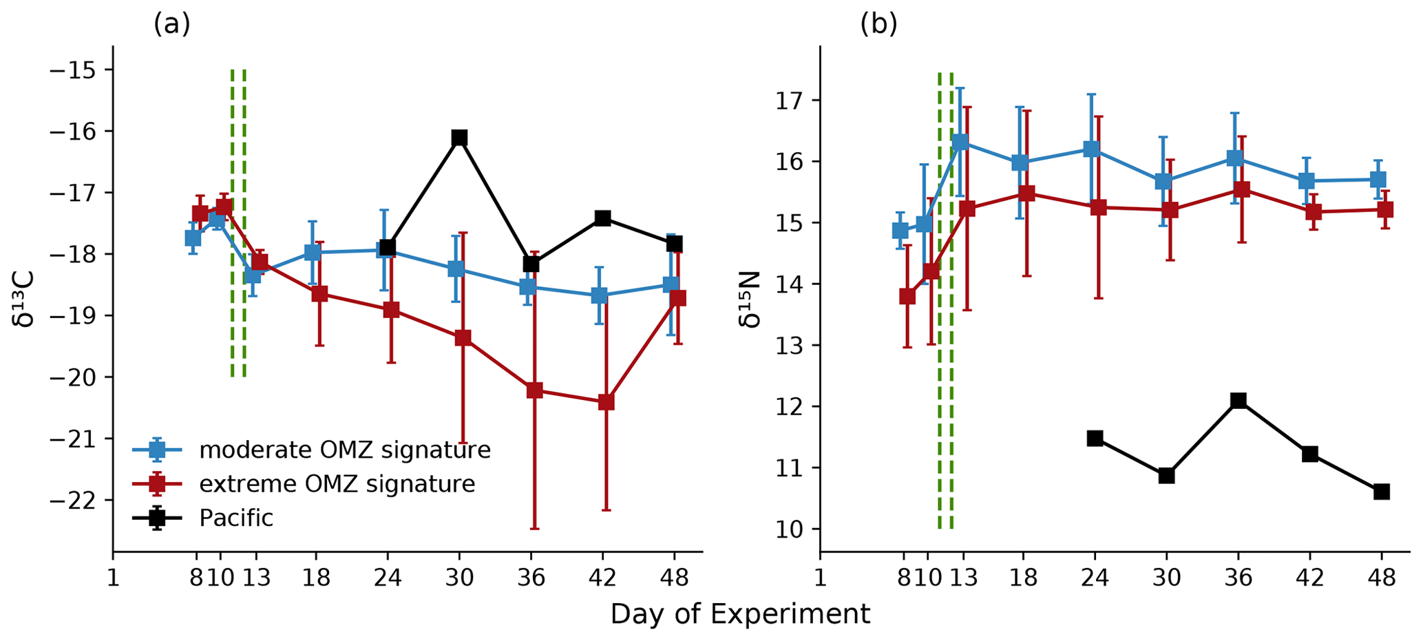
Figure 9 Temporal development averaged for the moderate and extreme treatments of δ¹³C (a) and δ¹⁵N (b) in copepods sampled in the eight mesocosms and the adjacent Pacific. Error bars depict 95 % confidence intervals. The green vertical dashed lines indicate the days of OMZ water additions. The experimental phase 1 lasted from day 1 until day 11–12, phase 2 until day 40, and phase 3 until experiment termination.

Table 5 Mean and standard deviation (SD) of cellular carbon, nitrogen, oxygen, and phosphorus content of dominant microzooplankton taxa as well as their molar ratios.

4 Discussion

4.1 Mesozooplankton dynamics

Our experiment coincided with a concurrent strong coastal El Niño, a situation of generally warmer waters and weaker upwelling conditions that favor small-sized zooplankton occurrence in the coastal upwelling areas (Ayón et al., 2011; Bertrand et al., 2011) that consequently dominated our MeZP community in the mesocosm bags at the start of the experiment. The MeZP community comprised various taxonomic groups with copepods dominating throughout the experiment in both the mesocosms and the surrounding Pacific; therefore, we focus our discussion on copepods. The four main genera were Paracalanus, Hemicyclops, Acartia, and Oncaea. Species of the genus Paracalanus, Acartia, and Oncaea are common in Peruvian coastal and neritic waters (e.g., Ayón et al., 2008a, 2011; Aronés et al., 2009), whereas the occurrence of the cyclopoid copepod Hemicyclops sp. off Callao has only been reported by Criales-Hernández et al. (2008). During our study, Hemicyclops sp. regularly occurred in the surrounding Pacific with different developmental stages including older copepodids.

The observed developmental delay of copepodids and adults and especially the very low abundance of nauplii may be a consequence of hypoxic conditions in the mesocosms below ∼10 m. Copepod nauplii were rare in the mesocosms, particularly after deep-water addition between day 18 and day 30 (<1 % or absent), although females of the sac-spawning Hemicyclops and also the less abundant Oncaea were frequently observed carrying egg sacs (personal observations). In contrast, except for the first days of the experiment, nauplii almost consistently comprised around 20 % of all copepod stages in the surrounding Pacific until day 30 and reached almost 80 % on day 36. This could be explained by advection of copepod populations carrying higher numbers of nauplii (Ayón et al., 2008b) or turbulence and upwelling keeping eggs in the oxygenated layer and promoting hatching. A lack of nauplii is also reflected in the development of copepodids and adults over the experimental duration and is particularly evident for Acartia sp. with adult copepods dominating the population almost over the entire study period. Despite species-specific tolerance levels, copepods generally respond to hypoxic conditions with avoidance (adults) and decreasing rates of survival, egg production, and population growth resulting in significant effects on population dynamics (e.g., Judkins, 1980; Marcus et al., 2004; Richmond et al., 2006; Ruz et al., 2017).

Eggs of Paracalanus sp., the dominant broadcast spawning (i.e., eggs released freely into the water column) copepod in the mesocosms, were probably particularly affected by hypoxia when sinking into low-oxygen waters. Field studies showed that maximum abundances of Paracalanus cf. indicus eggs in Mejillones Bay, Chile, were found in the oxygenated surface waters, whereas egg abundance decreased significantly from the oxygenated layer and the oxycline to the OMZ (Ruz et al., 2017). Sublethal and lethal hypoxia levels (<67 and <31 µmol L⁻¹ O₂, respectively; Auel and Verheye, 2007; Richmond et al., 2006) occurred in all mesocosms and the surrounding Pacific consistently throughout the study, where the oxycline was between 5 and 15 m and dissolved oxygen concentrations decreased at depth to <50 µmol L⁻¹ (Bach et al., 2020). Sinking velocities of Paracalanus parvus eggs determined in the lab and of P. cf. indicus determined in the field (Mejillones Bay, Chile) ranged 2.4–16.9 m d⁻¹ (Checkley, 1980a; Ruz et al., 2017). At a temperature range of 18–20 ^∘C, P. parvus nauplii hatch within 0.40–0.46 d, and the generation time of Paracalanus is about 18 d at 18 ^∘C (Checkley, 1980a). During our study, due to the coastal El Niño, surface temperatures usually varied between 20 and 22 ^∘C, exceptionally reaching 24 ^∘C between day 14 and day 22. Averaged over the entire mesocosm water column and all mesocosms, temperatures ranged between 18.4 and 20.2 ^∘C from days 1 to 38 and between 17.9 and 18.6 ^∘C thereafter (Bach et al., 2020). Thus, the experimental duration was long enough to expect Paracalanus eggs in the mesocosms. Eggs released at the mesocosms' surface would sink to 0.96–6.76 m depth within 0.4 d (9.6 h). Eggs released at greater depth would reach the oxycline and hypoxic layers faster, where development was likely halted or eggs may have suffered mortality. The accumulation of adults and a minimum contribution of copepodids around day 24, after oxygen concentrations in the mesocosms had decreased below 50 µmol O₂ L⁻¹ below 10 m depth (Bach et al., 2020), further support our notion of hindered egg development due to hypoxic conditions.

A late increase in copepod nauplii discernible in the mesocosm treatments on day 36 (extreme) and day 42 (moderate) might have resulted from a co-occurring deepening of hypoxic layers (<55 µmol L⁻¹) from ∼10 m to 14–15 m and slightly higher oxygen concentrations resulting from a phytoplankton bloom event facilitated through guanotrophication (Bach et al., 2020). Similarly, a short intrusion of oxygen-richer waters up to ∼10 m occurred in the adjacent Pacific, parallel to the small nauplii increase on day 30. Together with the concomitant increase in food availability this may have supported an increase in eggs and nauplii in both mesocosm treatments.

Upwelling is an important factor shaping copepod population dynamics operating through an optimal window of upwelling intensity that fosters copepod abundance and biomass, whereas increasing upwelling may be unfavorable for copepod populations (Escribano et al., 2012). This is in close connection with the fact that especially smaller copepods such as Paracalanus and Acartia require well-oxygenated waters for egg development and survival of early-stage copepods for population success (Ruz et al., 2017). Hence, our findings of failed egg and nauplii development strongly support these earlier notions and underline the importance of mesoscale variability and its implications for copepod reproduction in oxygenated waters and upwelling events, respectively.

4.2 Trophic relations

Exhausted inorganic nitrogen sources and the dominance of the mixotrophic and facultative osmotrophic dinoflagellate Akashiwo sanguinea in the phytoplankton community in most mesocosms (absent in M4) seem the most likely reasons for the extremely low GF of Paracalanus females during phase 2 of the experiment. Pigment contents determined for Paracalanus in our study were mostly an order of magnitude lower than those of Acartia, Pseudocalanus, and Temora from Danish waters (Kiørboe et al., 1985) and of Acartia off southern California (Kleppel et al., 1988). Paracalanus parvus prefers phytoplankton >5 µm over particulate matter as a food source but may also feed on dinoflagellates when these dominate phytoplankton biomass (Checkley, 1980a; Kleppel and Pieper, 1984). Furthermore, visual inspection of guts of Paracalanus females revealed that guts were often empty and that they were not feeding directly on phytoplankton.

The low GF is in accordance with the very low occurrence or absence of phytoplankton biomarker fatty acids determined in Paracalanus and Hemicyclops females in this study. Together, these point to the fact that development of these copepods depends on immediate food supply. Due to their very low lipid (TFA) levels, the fatty acid signatures of the copepods analyzed were largely dominated by biomembrane fatty acids (phospholipids), e.g., $\mathrm{16}:\mathrm{0},\mathrm{20}:\mathrm{5}(n-\mathrm{3})$, and $\mathrm{22}:\mathrm{6}(n-\mathrm{3})$. However, dietary signals of marker fatty acids are conserved in the storage lipids, i.e., in wax esters or triacylglycerols (Lee et al., 2006; Dalsgaard et al., 2003). The marker fatty acid $\mathrm{16}:\mathrm{1}(n-\mathrm{7})$ typical of diatoms decreased in Paracalanus females from initially ca. 5 % to 1% TFA–2 % TFA in phase 3, suggesting diatom ingestion only before or at the beginning of the experiment. However, Paracalanus females collected in the adjacent Pacific during phase 3 had higher $\mathrm{16}:\mathrm{1}(n-\mathrm{7})$ concentrations of 10 %, indicative of diatom feeding in the wild. In contrast, the fatty acid $\mathrm{18}:\mathrm{4}(n-\mathrm{3})$ typical of flagellates was not detected in significant amounts in any of the copepods. The near absence of wax esters (storage lipid) agrees with previous studies that egg production in the studied species is related to immediate food supply rather than a period prior to actual egg production, when energy reserves may have been accumulated (Checkley, 1980b).

Moreover, of the detected gut fluorescence no clear pheopigment peaks were identifiable with HPLC, which points to a high degree of degradation of fluorescent pigments found in the guts. Possibly, this “aged” gut fluorescence originated from ingestion of particulate matter, which could also explain why no particularly strong correlations existed between any of the phytoplankton groups and female abundance. The A. sanguinea bloom was associated with a marked increase in particulate organic matter and in the C:N ratio (from about 5–6 to 8–12) in the water column of most mesocosms (Bach et al., 2020). However, phytoplankton availability or dietary nitrogen (i.e., protein) is at times the direct limiting nutrient for egg production of Paracalanus (Checkley, 1980b). Hence, nutritional conditions for Paracalanus females were apparently insufficient in the mesocosms during phase 2, leading to low egg production and explaining the low numbers of nauplii found in the mesocosms.

Like Paracalanus, Hemicyclops may have lived at suboptimal conditions. Gut fluorescence was not detected in Hemicylops sp. The fatty acid composition of Hemicyclops females was analyzed only from day 30 onwards and was very similar to that determined for Paracalanus. Except for very low concentrations (2 % TFA–3 % TFA) of the diatom marker $\mathrm{16}:\mathrm{1}(n-\mathrm{7})$, no trophic marker fatty acids were identified and no fatty alcohols were determined; hence, no wax esters (storage lipid) were present. Correlation analysis suggested no particular food preference of Hemicyclops for any of the prevailing phytoplankton groups. The diet of Hemicyclops species with a coupled pelagic–benthic life cycle consists of microbenthos and meiobenthos, while detrital particles and also bacteria might be additional food sources (Itoh and Nishida, 2007, and references therein). Unfortunately, no studies are available on food preferences of H. thalassius. Although Hemicyclops is an egg-sac spawner, virtually no nauplii were found over the experimental runtime. Using a 100 µm mesh net, we may have missed the younger nauplii but should have captured the older naupliar stages (Itoh and Nishida, 2008). From the absence of nauplii despite the frequent presence of egg-sac-carrying females, we conclude that the Hemicyclops populations in the mesocosms, like Paracalanus, also lived at suboptimal conditions in terms of both nutrition and dissolved oxygen concentrations.

Isotopic signatures of zooplankton are determined by source and trophic fractionation. The latter is particularly the case for δ¹⁵N, for which an increase of 3 ‰–4 ‰ per trophic level is usually assumed for marine food webs (Cabana and Rasmussen, 1994; Minagawa and Wada, 1984; Peterson and Fry, 1987). Zooplankton δ¹⁵N values ranging approximately between 5 and 13 ‰ occur in (and close to) upwelling areas (e.g., Rau et al., 2003; Schukat et al., 2014; Teuber et al., 2014), whereas lower zooplankton δ¹⁵N values (∼2 ‰–4 ‰) were found in regions with a high diazotroph contribution to the pelagic food web (Hauss et al., 2013; Sandel et al., 2015). δ¹⁵N values of zooplankton (copepods) in the mesocosms following a simulated upwelling pulse were rather high (∼13–17 ‰) compared to the δ¹⁵N (mean 7.6 ‰) measured by Espinoza et al. (2017) for bulk copepod samples of the HCS. The δ¹³C ratio of copepods from M4 differed profoundly from the other mesocosms in phase 2 (day 13–36). The decrease in δ¹³C seems to correlate with an increase in Chlorophyceae, which made up >90 % of the phytoplankton community on day 36 (Bach et al., 2020). Turnover time of δ¹³C in copepods varies from days to weeks (Gentsch et al., 2008). An increase in Chlorophyceae and following constant supply should be seen in the C signal of the copepods after several days. Also, in contrast to the other mesocosms, δ¹⁵N was generally lower in M4 in the first two phases. M4 was the only mesocosm lacking the dinoflagellate Akashiwo sanguinea (Bach et al., 2020). Mixotrophy by this flagellate could thus have led to increased nitrogen fractionation in the other mesocosms.

A comparison of δ¹⁵N among different studies without clearly defined baseline values (phytoplankton) is difficult, as the δ¹⁵N baseline is strongly affected by the variability in the intensity of the OMZ along the Peruvian coast (Mollier-Vogel et al., 2012). A recent study by Massing et al. (2022) revealed an enrichment in δ¹⁵N of ∼5 ‰ for several copepod species of the HCS from north (8.5^∘ S) to south (16^∘ S). The δ¹⁵N ratios of seston also increased with depth, i.e., between seston from surface oxygenated waters and the OMZ. Dissolved inorganic nitrogen taken up by phytoplankton often creates the basis of the isotopic composition of the whole food web (Argüelles et al., 2012). Under anoxic conditions in OMZs, a preferred uptake of the lighter isotope by denitrifiers leads to elevated δ¹⁵N in the remaining nitrate (Granger et al., 2008). OMZs such as the strong and shallow one in the northern HCS are thus sites of intense nitrogen loss (Ward et al., 1989), leading to an increase in δ¹⁵N baseline values (Sigman et al., 1999; Graham et al., 2010). The higher δ¹⁵N of copepods within the mesocosms can therefore be a result of or may be explained by the source water injection to the mesocosms, which was reduced in oxygen and most likely enriched in δ¹⁵N. Starvation would lead to loss of body mass and preferential metabolism of the lighter isotope, with a resulting increase in delta values for both tracers (Hobson et al., 1993; Gannes et al., 1997).

5 Conclusions

Our results provide interesting insight on the response of a zooplankton community and their trophic relations to an upwelling event with OMZ waters. In particular GF and fatty acid compositions revealed that after deep-water addition feeding of dominant copepods on autotrophic food (diatoms) was insignificant and copepods lived from “hand to mouth”. This may point to an important role of heterotrophic and mixotrophic organisms as a food source for copepods. Though egg production was not determined in our study, we assume that the lack of nauplii during most of the experiment duration was preceded by failed production and/or development of copepod eggs and nauplii due to both prevailing hypoxic and insufficient nutritional conditions in the mesocosms. With respect to hypoxia, we conclude that a few meters of oxygenated waters more or less may make a huge difference for copepod secondary production. With respect to nutrition, changing N:P ratios of upwelled water may further contribute to negatively impact copepod reproductive success, as the availability of nitrogen-rich food sources is important for reproductive output of copepods relying on immediate food supply for egg production (Checkley, 1980b). Hence, increasing upwelling intensity and shoaling of the OMZ as projected for EBUS under ocean warming (Stramma et al., 2008; Schmidtko et al., 2017) may have severe consequences for mesopelagic food webs, trophic transfer, and fish production in the HCS (Ayón et al., 2008b; Aronés et al., 2019). Future studies should focus on the nutritional condition and fecundity of the copepods, the importance of heterotrophic food sources in the nutrition of copepods, and microzooplankton grazing in the food web. Measures of nutritional condition would also help to strengthen interpretation of isotopic signatures in relation to starvation of organisms. Together, these would add further detail to a more comprehensive understanding of the response of plankton communities and their trophic links to the projected varying impact of upwelling intensity and/or frequency of OMZ waters off Peru.