Diurnal versus spatial variability of greenhouse gas emissions from an anthropogenically modified lowland river in Germany

Greenhouse gas (GHG) emissions from rivers are globally relevant, but quantification of these emissions comes with considerable uncertainty. Quantification of ecosystem-scale emissions is challenged by both spatial and short-term temporal variability. We measured spatio-temporal variability of CO₂ and CH₄ fluxes from a 1 km long reach of the lowland river Elbe in Germany over 3 d to establish which factor is more relevant to be taken into consideration: small-scale spatial variability or short-term temporal variability of CO₂ and CH₄ fluxes.

GHG emissions from the river reach studied were dominated by CO₂, and 90 % of total emissions were from the water surface, while 10 % of emissions were from dry fallen sediment at the side of the river. Aquatic CO₂ fluxes were similar at different habitats, while aquatic CH₄ fluxes were higher at the side of the river. Artificial structures to improve navigability (groynes) created still water areas with elevated CH₄ fluxes and lower CO₂ fluxes. CO₂ fluxes exhibited a clear diurnal pattern, but the exact shape and timing of this pattern differed between habitats. By contrast, CH₄ fluxes did not change diurnally. Our data confirm our hypothesis that spatial variability is especially important for CH₄, while diurnal variability is more relevant for CO₂ emissions from our study reach of the Elbe in summer. Continuous measurements or at least sampling at different times of the day is most likely necessary for reliable quantification of river GHG emissions.

1 Introduction

1.1 Greenhouse gas emissions from rivers

Rivers are a globally relevant source of greenhouse gases (GHG) (Battin et al., 2023; Raymond et al., 2012; Rocher-Ros et al., 2023; Stanley et al., 2023). It is currently estimated that rivers globally emit about 2 Pt CO₂ yr⁻¹ (Liu et al., 2022) and 30.5 ± 17.1 Tg CH₄ yr⁻¹ (Rosentreter et al., 2021). However, these estimates suffer from considerable uncertainty. Aquatic GHG emissions actually generate considerable uncertainty among global GHG assessments (IPCC, 2021). Reducing uncertainty in aquatic GHG budgets is important in order to improve biogeochemical models and climate prediction(s). Uncertainties result from a general lack of data as well as from the methods used for budgeting aquatic GHG emissions.

1.2 Traditional method for budgeting

Bottom–up approaches for quantifying riverine GHG fluxes are typically based on GHG concentrations measured in a restricted number of water samples. GHG fluxes between water and atmosphere (J) are calculated from concentrations (C_water) measured in water samples or calculated from other parameters of the carbonate system (pH, alkalinity, and/or dissolved inorganic carbon (DIC)) and estimated gas transfer velocities (k) (Raymond et al., 2013) multiplied by water surface area (A) (Eq. 1):

$$\begin{array}{}\text{(1)}& J=kx\left(C_{\mathrm{water}}-C_{\mathrm{atm}}\right)\times A\left[\mathrm{mol}{\mathrm{h}}^{-\mathrm{1}}\right],\end{array}$$

were C_atm is the concentration in water which is in equilibrium with the atmosphere. The gas transfer velocity is a physical parameter describing diffusive gas exchange at the water surface and is typically estimated from hydrodynamic parameters such as flow velocity, slope, and/or bottom roughness (Raymond and Cole, 2001). Typical datasets contain weekly to monthly concentration data from a small number of sites along a specific river (Stanley et al., 2023). GHG fluxes can also be directly measured by floating chambers. However, these measurements are laborious and prone to experimental artefacts if not carried out carefully (Lorke et al., 2015). Water surface areas are typically estimated by using river width based on empirical relations (Raymond et al., 2013) or for larger rivers using remote sensing data (Palmer and Ruhi, 2018). These approaches are suitable for covering seasonal dynamics as well as large-scale spatial patterns along larger rivers. However, recent research has indicated considerable short-term temporal and small-scale spatial variability of riverine GHG fluxes, which poses challenges for budgeting and upscaling.

1.3 Short-term temporal variability

There is contrasting evidence for the occurrence of diurnal fluctuations of CO₂ in larger rivers (Ishaque, 1973; Haque et al., 2022). The advent of reliable and affordable probes to continuously measure GHG concentrations revealed considerable diurnal fluctuations of CO₂ in streams (Gómez-Gener et al., 2021). Because the balance between photosynthesis and respiration depends on light, CO₂ fluxes are typically elevated at night (Attermeyer et al., 2021). Thus, CO₂ emission estimates relying only on discrete water samples taken during daylight hours often significantly underestimate true emissions.

Whereas diurnal fluctuations of CO₂ are well documented, there is little knowledge concerning the short-term variability of CH₄ (Stanley et al., 2016).

1.4 Small-scale spatial variability

While there are several studies investigating spatial variability in streams, much less is known about spatial variability of GHG emissions from larger rivers. Rivers contain various habitat types: these are either natural or have anthropogenic modifications. Channelization and disconnection of rivers from their floodplain decrease spatial heterogeneity (Wohl and Iskin, 2019) and most likely also affect GHG fluxes (Machado dos Santos Pinto et al., 2020). However, anthropogenic modifications do not only reduce habitat diversity. Several European rivers were modified by building groynes in the 19th century with the primary goal of concentrating the water into the main river and of improving river flow and navigability (Pusch and Fischer, 2006). Consequently, the flow velocity is lower within the groyne fields, leading to increased sedimentation (Kleinwächter et al., 2017). Thus, groynes increase habitat diversity compared to straight, channelized rivers but they decrease diversity compared to a natural shoreline. In the Elbe, there are no groynes until river km 120 according to German kilometration however, they dominate the shoreline downstream from that point (Fig. 1b). A recent study presents evidence that the still water areas between such groynes are a source of CH₄ resulting in lateral CH₄ gradients (Bussmann et al., 2022). Ignoring these gradients significantly underestimates total CH₄ emissions. Sediment is the predominant source of CH₄ in streams (Stanley et al., 2016), and spatial variability of CH₄ production in rivers is known to be controlled by sediment deposition (Maeck et al., 2013).

A typical feature of rivers is their fluctuating discharge resulting in fluctuating water levels. Thus, depending on discharge, certain parts of rivers are temporarily drying up. It has been shown that these dry river areas emit disproportionally high amounts of CO₂ into the atmosphere (Gómez-Gener et al., 2015). Ignoring dry areas in river GHG budgets may lead to a significant underestimation of GHG emissions (Marcé et al., 2019). Depending on their elevation, such dry river sediments can be quite heterogeneous with respect either to substrate type (sand versus mud) or to the occurrence of temporary vegetation (Bolpagni et al., 2019). Recent research indicates considerable spatial variability and temporal dynamics of dry river GHG fluxes (Mallast et al., 2020; Koschorreck et al., 2022).

1.5 Aim of this study

We expected that small-scale spatial and diurnal variability would need to be considered for budgeting GHG emissions from rivers. The ideal approach would thus be to perform high-frequency measurements at a large number of sites. However, this is simply not possible and thus there is a trade-off between frequency and spatial coverage of measurements. In this study, we aim to answer the question, “What is more important for budgeting and/or upscaling GHG emissions from rivers: small-scale spatial or short-term temporal variability?” We hypothesize that the answer to this question depends on the gas: we expected spatial heterogeneity to be more relevant for CH₄ fluxes and temporal variability to be more relevant for CO₂. To test this hypothesis, we measured CH₄ and CO₂ fluxes in different habitats within a typical reach of the lowland river Elbe in Germany during a 3 d campaign. The study was designed to cover a typical low-discharge summer situation when both habitat diversity and biological activity in the river were expected to be the highest.

2 Materials and methods

2.1 Study site

Investigations were performed at a 1 km long reach of the 8th-order river Elbe at Tangermünde located in the middle part of the river in Germany at river km 388 according to German kilometration (Fig. 1a). The reach is typical for the middle Elbe, which is characterized by groyne fields (Fig. 1b) between km 120 and 580. Measurements were made in late summer during 18–22 August 2022. Discharge varied between 189 and 197 m³ s⁻¹ during that period, which was below the mean low discharge of 235 m³ s⁻¹ (Fig. 2).

We separated the river's water surface into three distinct habitats: the middle of the river, the sides of the river, and the area between groynes (groyne fields). The groyne fields extend from the riverbank to a virtual line connecting the heads of the groynes. We defined the side areas as extending from the outer boundary of the groyne fields 15 m into the river (about 10 % of river width). Visual inspection confirmed that 15 m fully included the turbulent areas below the groyne heads. The reach studied here had 10 groynes at both banks, extending up to 60 m into the river. The distance between the groynes was 80 ± 10 m. The area between the groynes was partly dry. These dry areas featured three typical habitats: muddy areas and sandy beaches without and with terrestrial vegetation (Fig. 1c and Fig. S1 in the Supplement).

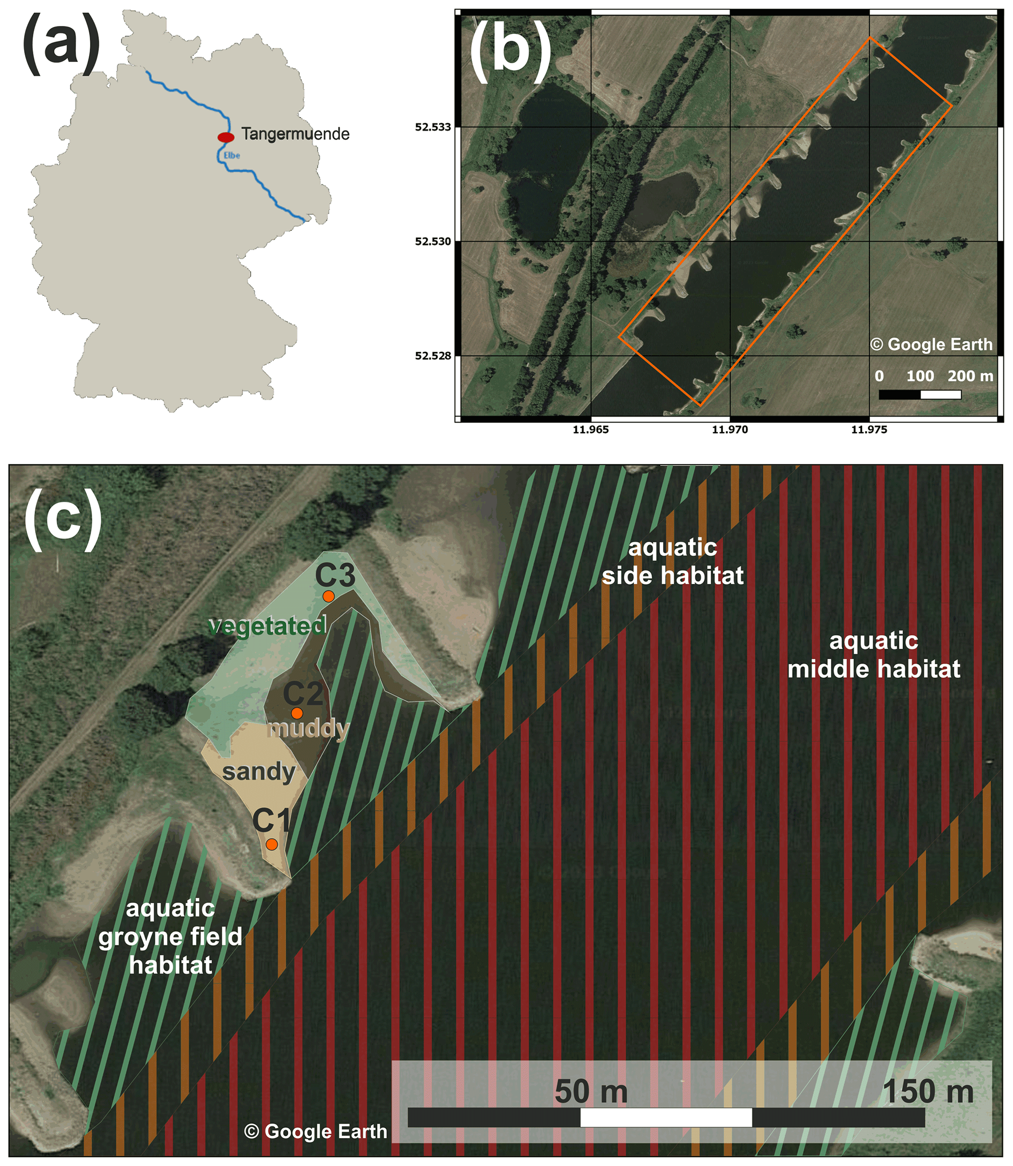
Figure 1 Location of the investigation site Tangermünde (red dot) in Germany at the Elbe, at river km 388 according to German kilometration (a). Top view of the sampling reach with groyne fields (orthophotograph source: Google Earth, GeoBasis-DE/BKG, date of recording 6 August 2020), flow direction to north-east, study area marked by orange lines (b). Detailed view of the study area with indication of habitat types (c). The groyne field is divided into an aquatic habitat and a terrestrial habitat with partially dry fallen sediments, which are divided into sandy areas (location of soil flux chamber C1), muddy areas (chamber C2), and vegetated areas (chamber C3) (orthophotograph source: Google Earth, GeoBasis-DE/BKG, date of recording 6 August 2020, © Google Earth, see also Fig. S1).

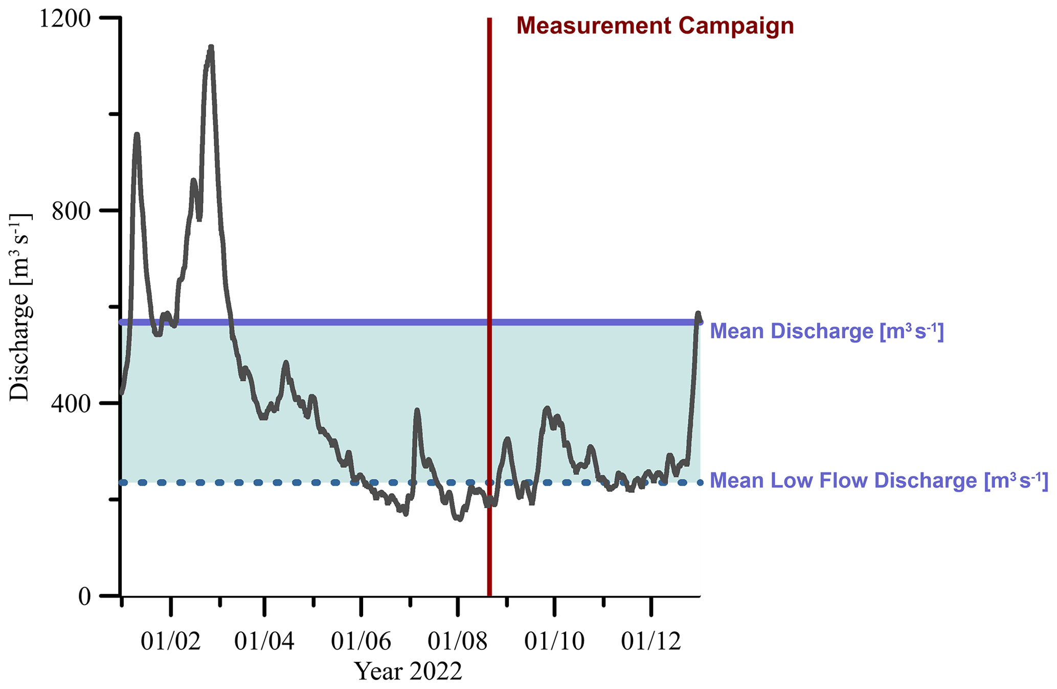
Figure 2 Discharge of the river Elbe at gauge Tangermünde during 2022 (German Federal Waterways and Shipping Administration). The blue area marks the range between mean low-flow discharge (annual mean of the lowest discharge of each month) and mean discharge; the red area marks the period of the sampling campaign.

2.2 Aquatic measurements

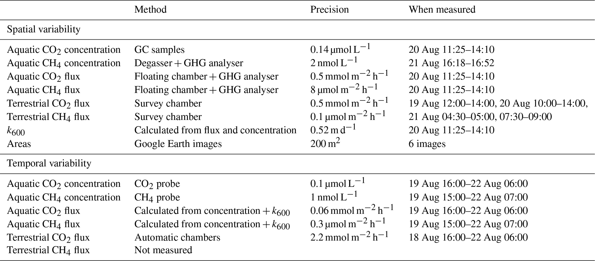
Table 1 provides an overview of the different methods used to assess GHG concentrations and fluxes.

2.2.1 Hydrodynamics and basic physicochemical measurements

Flow velocity profile measurements were conducted at the study site at Tangermünde on 19 August 2022. We deployed a four-beam 1200 kHz acoustic Doppler current profiler (ADCP; Teledyne RD Instruments, TRDI) from an inflatable boat. The vertical resolution of water velocities was 0.25 m (25 cm bins), and the sampling frequency was approximately 2 Hz. In total, eight transects of flow velocity and water depth were measured using four to five replicates at each transect (Fig. S3). Depth-averaged velocities (U) were calculated from the measured portion of the water column, neglecting the unmeasured upper and lower portion of the water column (see Fig. S3). Global positioning system (GPS) position data were collected using a GPS tracker (Garmin International, Schaffhausen, Switzerland) with a frequency of 1 s.

Basic hydrographic parameters (temperature, conductivity, oxygen, pH, turbidity, and chlorophyll) were determined with a PocketFerryBox system (4H-Jena, Kiel, Germany) and a multiparameter probe (EXO2, YSI). The water supply for both sensors was the ship's duct with direct water supply from the RV Albis. We mapped basic hydrographic parameters with the RV Albis meandering between the western and eastern groyne heads on 19 August 2022. Due to the size of the ship, it was not possible to enter near-shore areas and groyne fields. From 19 to 22 August 2022, the RV Albis was anchored at the pier in Tangermünde and measured the hydrographic parameters at the same position continuously for 63 h.

2.2.2 Aquatic GHG measurements

To assess the spatial pattern of aquatic GHG fluxes, aquatic GHG fluxes were measured from an inflatable boat using a floating chamber connected to a portable FTIR analyser (GASMET DX4000, Gasmet Technologies, Finland) as explained by Lorke et al. (2015). We used exactly the same rectangular drifting chamber (area 0.098 m², height 0.15 m) as Lorke et al. (2015) for the river Bode. For each measurement the chamber was deployed from a drifting boat for 2–5 min. Fluxes were calculated from the linear change of CO₂ and CH₄ mixing ratios in the chamber. A water sample for later gas chromatography (GC) analysis was taken during each flux measurement. Surface water samples of 30 mL were taken with 60 mL syringes, and 30 mL of ambient air was added to the syringes, which was then vigorously shaken for 1 min. The equilibrated headspace was then transferred to pre-evacuated Exetainers and the equilibration temperature was measured in the remaining water sample.

Dissolved CH₄ concentrations were mapped with a dissolved gas extraction unit and a laser-based analytical greenhouse gas analyser (GGA; both Los Gatos Research, USA) on an inflatable boat. The degassing unit withdrew water from the water basin or directly from surface water at 1.2 L min⁻¹. CH₄ was extracted from the water via a hydrophobic membrane, and hydrocarbon-free carrier gas was on the other side of the membrane (nitrogen, at 0.5 L min⁻¹). The carrier gas with the extracted CH₄ was then directed to the inlet of the gas analyser. The time offset between the water intake and stable recording at the GGA was determined beforehand in the laboratory. To convert the relative concentrations (ppm) given by the GGA to absolute concentrations (nmol L⁻¹), discrete water samples were obtained at least every hour. The CH₄ concentration in these bottles was determined using the headspace method and GC analysis. The range of concentrations from the water samples used for calibration was rather narrow (178–258 nmol L⁻¹); thus we used a conversion factor (water sample conc./ppm from GGA), which was 88.7 ± 23 nM ppm⁻¹) (Table S1).

For high-spatial-resolution measurements the degassing unit and GGA were set up in a small rubber boat with a 5 L nitrogen tank and a car battery. The water inlet of the degasser was fixed to a bar and submerged to approx. 20 cm water depth. We entered each groyne field from the north and kept the boat at the groyne heads for approximately 2 min (against the current) and then entered the following groyne field as far as possible (Fig. 3).

For continuous measurements of dissolved CO₂ and CH₄, an optical AMT sensor (AMT, Analysenmesstechnik GmbH, Rostock, Germany) and a CONTROS sensor (4H-Jena, Jena, Germany) were deployed in the duct of the Albis. The CO₂ sensor provided data as parts per million (ppm) which were converted to concentrations (µmol L⁻¹) according to the solubility at the respective temperature (UNESCO/IHA, 2010). The CH₄ mixing ratio (ppm) values of the CONTROS sensor were converted to absolute concentrations (µmol L⁻¹) by relating them to water samples measured with a GC, similar to the values from the GGA (Los Gatos Research). The conversion factor here was 0.06 µmol L⁻¹ ppm⁻¹. Probes were checked in the laboratory prior to deployment by comparing probe readings with concentrations measured by GC and/or a membrane equilibrator connected to a nondispersive infrared (NDIR) analyser, as explained in Koschorreck et al. (2021).

2.3 Terrestrial and atmospheric measurements

The mixing ratio of CO₂ in the atmosphere and other meteorological parameters was continuously measured by a senseBox. The senseBox system is a toolkit developed in the framework of Citizen Science Projects for environmental data collection funded by the German Federal Ministry of Education and Research. It consists of an open-source microcontroller unit which can be connected to various environmental sensors (Bartoscheck et al., 2019). The senseBox was equipped with a GPS sensor, an environmental sensor measuring air temperature, relative humidity, and air pressure, and a CO₂ sensor determining the air CO₂ mixing ratio. The senseBox was installed at the RV Albis and measured the atmospheric conditions every 5 min.

The spatial variability of CO₂ and CH₄ fluxes at terrestrial sediments was measured with the laser-based trace gas analyser LI-7810 (LI-COR Biosciences, Lincoln, USA) in combination with a closed chamber (LI-COR Smart Chamber). Soil gas fluxes were calculated from the temporal gas concentration change taking into consideration the chamber volume and the surface area of the soil area covered by the chamber. For each sampling point, the change in gas concentration in the closed chamber was determined after a purging period at a 1 s sampling interval during the 2 min observation time. Fluxes were calculated using the linear fitting approach of the SoilFluxPro software (LI-COR Biosciences). Based on our own long-term tests with the system, soil flux detection limits of ± 0.36 mmol m⁻² h⁻¹ were determined for CO₂ (corresponding to a change of 2 ppm CO₂ during a closure period of 2 min) and of ± 0.072 µmol m⁻² h⁻¹ for CH₄ (corresponding to a change of 0.6 ppb CH₄ during a closure period of 2 min). To assess spatial variability, we measured GHG fluxes at five sandy, five muddy, and nine vegetated sites (Fig. S2). Muddy and sandy areas were free of vegetation and could be clearly distinguished from vegetated zones, which were widely covered by typical herbaceous plants such as Persicaria, Inula britannica, and Xanthium strumarium.

To cover the temporal dynamics of terrestrial CO₂ fluxes, three opaque automatic chambers (CFLUX-1 Automated Soil CO₂ Flux System, PP Systems, Amesbury, Massachusetts, USA) were installed at a sandy site, a muddy site, and a sandy site with herbaceous vegetation (Figs. 1d, S2). The chambers measured CO₂ fluxes once every hour. Each flux measurement lasted for 5 min, and the chambers were open for 55 min between flux measurements. CO₂ fluxes were calculated from the linear increase of CO₂. The detection limit for terrestrial CO₂ fluxes was 0.08 mmol m⁻² h⁻¹. The reliability of the CO₂ measurement in the automatic chambers was checked by comparing the atmospheric background concentrations measured independently by the three automatic chambers. Each chamber was equipped with a soil moisture and temperature probe (Stevens HydraProbe, Stevens Water Monitoring Systems, Portland, Oregon, USA).

Light intensity was measured at Magdeburg (50 km from Tangermünde) as PAR [µmol m⁻² s⁻¹] using an LI-190R Quantum Sensor (LI-COR Biosciences).

Table 1 Overview of methods used to measure different parameters. Precision is defined as 2 times the standard deviation of at least 10 consecutive measurements (5 replicate image analyses per area). The precision of the terrestrial flux measurements based on survey chamber investigations is site specific and determined using the fitted linear gas concentration curves.

2.4 Laboratory analyses

CO₂ and CH₄ concentrations in gas samples were measured with a gas chromatograph (GC) (SRI 8610C, SRI Instruments Europe GmbH, Bad Honnef, Germany). The GC was equipped with a flame ionization detector and a methanizer, which allowed for simultaneous measurement of CO₂ and CH₄ with an uncertainty of < 5 %. Dissolved gas concentrations were calculated using temperature-dependent Henry coefficients (UNESCO/IHA, 2010). CO₂ concentrations were corrected for alkalinity as described in Koschorreck et al. (2021).

2.5 Calculations and statistics

Gas transfer coefficients were calculated from CH₄ fluxes measured by the floating chambers divided by the difference between actual and equilibrium CH₄ concentrations. Equilibrium CH₄ concentrations were calculated from the mean measured atmospheric CH₄ mixing ratio (2.5 ppm) using temperature-dependent Henry coefficients from Sander (2015); (Koschorreck et al., 2021). The thus-determined $k_{{\mathrm{CH}}_{\mathrm{4}}}$ was converted to k₆₀₀ and $k_{{\mathrm{CO}}_{\mathrm{2}}}$ using Schmidt numbers according to UNESCO/IHA (2010). We did not use CO₂ data for k₆₀₀ calculations because the CO₂ concentration was close to equilibrium resulting in large uncertainties in the calculation of k₆₀₀.

Probe measurements of CO₂ and CH₄ concentrations measured at RV Albis were converted to fluxes using the measured gas transfer velocity of k₆₀₀ = 5.2 m d⁻¹ (Table 2). This assumes that k₆₀₀ at the probe site was equal to the mean k₆₀₀ measured at the side habitat. For CO₂ fluxes, we used the measured atmospheric CO₂ mixing ratios while for CH₄ we used a constant atmospheric mixing ratio of 2.5 ppm. k₆₀₀ was converted to kCO₂ and kCH₄, as explained earlier.

Fluxes from different habitat types were compared by pairwise Wilcoxon tests. Fluxes during the day were compared with fluxes during the night using Wilcoxon rank-sum tests. For statistical analysis, all high-frequency data were transformed to hourly data by calculating the mean values of data available between 30 min before and 30 min after the full hour. Time series data were log transformed after checking for normality by using Shapiro–Wilk tests. Since we sometimes observed slightly negative fluxes, fluxes were corrected by adding the most negative flux to all flux data before log transformation. The significance of the linear correlation of log-transformed fluxes with drivers was checked through F tests (p<0.05). Linear mixed models to explain GHG fluxes from combinations of predictors were compared based on their Akaike information criterion (AIC; Bates et al., 2015). To consider site-specific correlations, we added site as a random factor to our statistical model. All statistical analyses were done with R (R Core Team, 2016).

3 Results

3.1 Hydrodynamic and climatic conditions

Our study was conducted during a typical summer low-water situation. At the gauge level of 134 cm (on 6 August 2022, when the orthophotograph in Fig. 1 was taken), 9 % of the study area was not covered by water (Table 2). Flow velocity in the river was relatively uniform at around 0.65 m s⁻¹ while within the groyne fields flow velocity was significantly lower (Table 2). The minimum and maximum measured flow velocities were 0.007 and 1.05 m s⁻¹, respectively, and the minimum and maximum water depths were 0.45 and 3.1 m, respectively. Water was flowing rather smoothly without larger waves, but we observed more turbulent conditions downstream of the groyne heads. The mean water depth was 1.82 m with the most shallow parts but also the deepest parts in the groyne fields (maximum depth 3.1 m). The water level rose by 10 cm over the 3 d of our study. Weather conditions were rather constant during our study period, predominantly sunny, with 5.6 mm of rainfall during the first night (on 19 August 2022 until 06:00 local time). Air temperature fluctuated between 12.4 and 32.2 °C, and low wind speeds of 0.3 ± 0.6 m s⁻¹ were recorded (Fig. S7). Water temperatures were evenly distributed (23.3 ± 0.04 °C, measured between 19 August 2022 at 14:00 and 22 August 2022 at 08:00). Electrical conductivity of the water on the western shore and within the western groyne fields was about 200 µS cm⁻¹ higher than on the eastern shore (Fig. S4). This conductivity gradient has been attributed to the salty inflow of river Saale 97 km upstream of our sampling site (Weigold and Baborowski, 2009). This slight difference in conductivity most probably does not affect microbial GHG production, but it indicates limited lateral mixing of river water even over a large distance.

3.2 Spatial variability

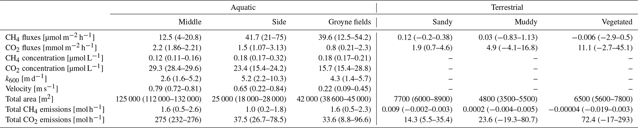
GHG concentrations and fluxes differed between habitats and also between the two gases, CO₂ and CH₄ (Table 2). The water was over-saturated both with CO₂ and CH₄, resulting in positive fluxes (= emissions to the atmosphere). The flux of CO₂ from the water surface was 2 orders of magnitude higher than the CH₄ flux. Dissolved CO₂ concentrations were highest in the middle of the river and decreased towards the side. An opposite pattern was observed for CH₄, which was higher at the sides and within the groyne fields than in the middle of the river (Fig. 3). Since the gas transfer velocity k₆₀₀ was twice as high at the sides compared to the middle of the river, CH₄ fluxes were significantly higher at the sides and in the groyne field compared to the middle of the river. We never observed ebullition in our chamber measurements. Since higher CO₂ concentrations in the middle of the river were compensated by lower k₆₀₀ values, fluxes of CO₂ did not differ significantly between aquatic habitats (Fig. 4). Sediment incubations (Methods in the Supplement) confirmed that CH₄ was mainly produced in the sediment. In sediment samples from a groyne field, CH₄ was produced with a rate of 2095 ± 2781 nmol L⁻¹ h⁻¹. Oxic water samples also produced CH₄ with a low rate of 1.73 ± 0.5 nmol L⁻¹ h⁻¹.

The dry habitats had higher CO₂ fluxes but lower CH₄ fluxes compared to the aquatic sites. Dry CO₂ fluxes showed a large variability within habitats and were highest at vegetated sites and very low at the sandy sites (Fig. 4). Dry CH₄ fluxes, by contrast, were more than 2 orders of magnitude lower, in some cases even slightly negative (Table 2), and only small differences between habitats were observed.

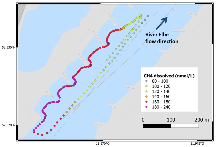
Figure 3 Concentrations of dissolved CH₄ in the water measured continuously with a mobile gas extraction unit connected to a GHG analyser. Measurements were carried out from an inflatable boat on 21 August 2022 between 16:18 and 16:51 local time. CO₂ was also measured with the GHG analyser but data were not used because gas extraction was different for CH₄ and CO₂ and the system was optimized for CH₄.

Table 2 GHG fluxes and their regulating factors in different habitat types. Flux data from floating chamber measurements, CH₄ concentration measured by a membrane equilibrator connected to a portable GHG analyser (data from Fig. 3), CO₂ concentration analysed by GC, and velocity measured by ADCP. Areas were manually extracted from Google Earth images. All data are median (range). CH₄ fluxes are given in µmol m⁻² h⁻¹ and CO₂ fluxes in mmol m⁻² h⁻¹. Original data of terrestrial fluxes are published in Koedel and Schütze (2023).

3.3 Temporal variability

Continuous measurements of aquatic GHG concentrations (Fig. S5) and water physicochemical variables (Fig. S6) were carried out over a period of 2.5 d at the side of the river. Water temperature (median 22.6 °C; range 21.7–23.7 °C), pH (median 8.0; range 7.3–8.3) and oxygen (median 97.9 %; 87.5 %–117.8 % saturation) showed a clear daily pattern, with the lowest values in the early morning (05:00–06:00), while conductivity was rather constant (median 1260 µS cm⁻¹; range 1146–1381 µS cm⁻¹; Fig. S6).

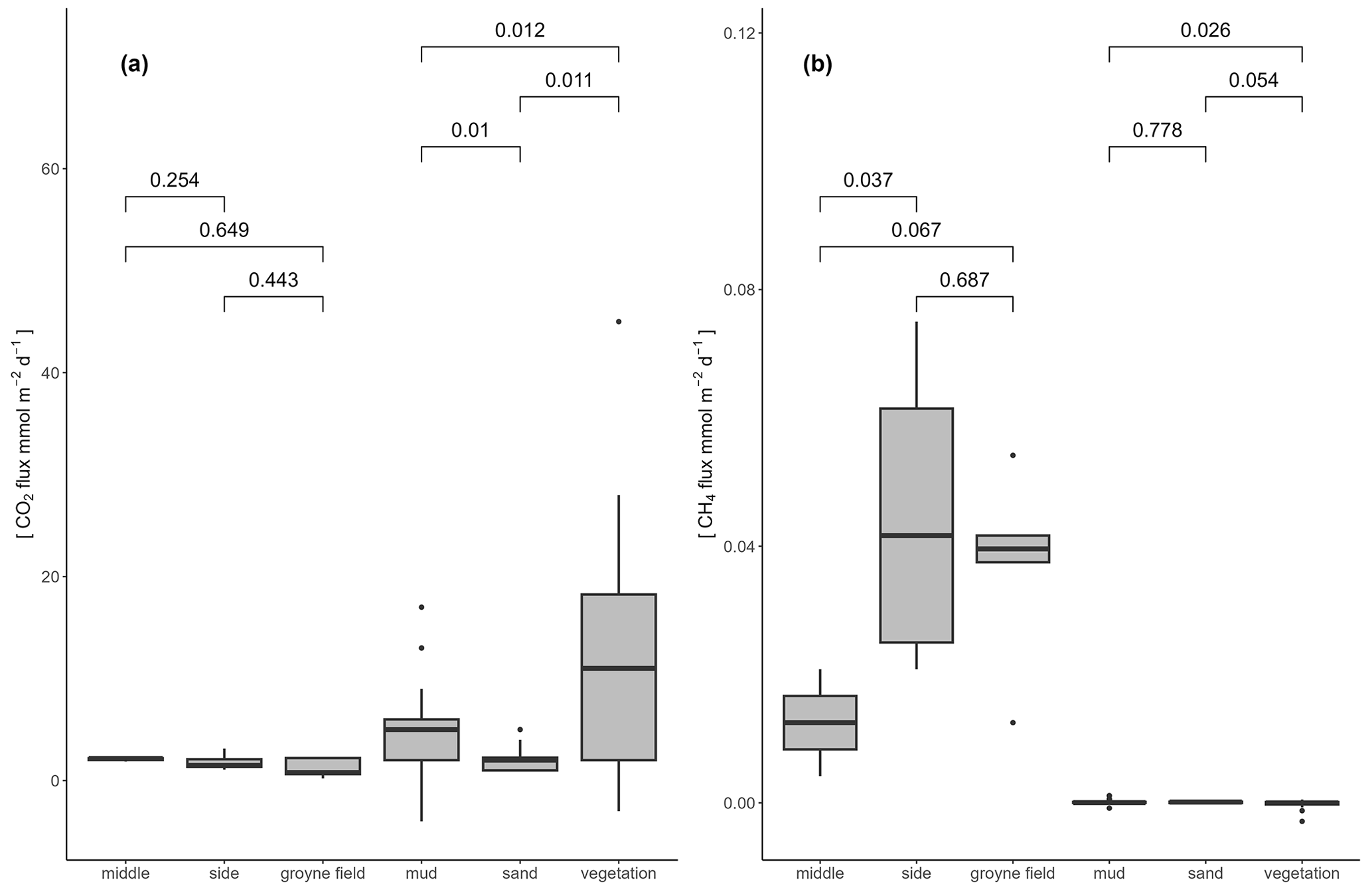
Figure 4 Boxplots comparing CO₂ flux (a) and CH₄ flux (b) in different habitat types. Numbers within the plots indicate p values of pairwise comparisons using Wilcoxon tests (same data as in Table 2).

Aquatic CO₂ concentrations showed a clear diurnal cycle with rising concentrations during the night and decreasing concentrations during the day. The diurnal amplitude of the resulting flux spanned about 5 mmol m² h⁻¹ with maximum fluxes around 05:00 and minimum fluxes around 19:00 (blue line in Fig. 5a). In contrast to CO₂, the CH₄ concentration and the flux did not change with time (Fig. 5b).

At the dry sites, diurnal pattern of CO₂ fluxes were apparent, but these patterns differed between habitat type. At the vegetated site, a pattern similar to the aquatic site was observed, only phase shifted. The highest fluxes were found around noon, while the minimum flux was before sunrise (green line in Fig. 5a). The mud site did not show such a sinus-like pattern but a two-state pattern: the site switched from constant fluxes during the night to constant CO₂ uptake during the day (red line in Fig. 5a). No diurnal variability of CO₂ fluxes was observed at the sandy site (yellow line in Fig. 5a). The CH₄ flux data from the dry sites do not enable visualization of diurnal variability, but the data (dots in Fig. 5b) at least do not show any temporal trend during the day.

CO₂ fluxes from the mud and the vegetated site showed a decreasing trend during our study. At the muddy site, this trend was associated with increasing sediment moisture (Fig. 5c), which was obviously caused by the rising water level of the river (Fig. 5d) – on 21 August the flux chamber was only 1 m from the water line. At the other dry sites, no trend of sediment moisture was visible, but sediment temperature during the day tended to increase throughout the study (Fig. 5c). There was light rain during the first night (Fig. 5d) which resulted in a slight increase in sediment moisture as well as in CO₂ flux only at the vegetated site.

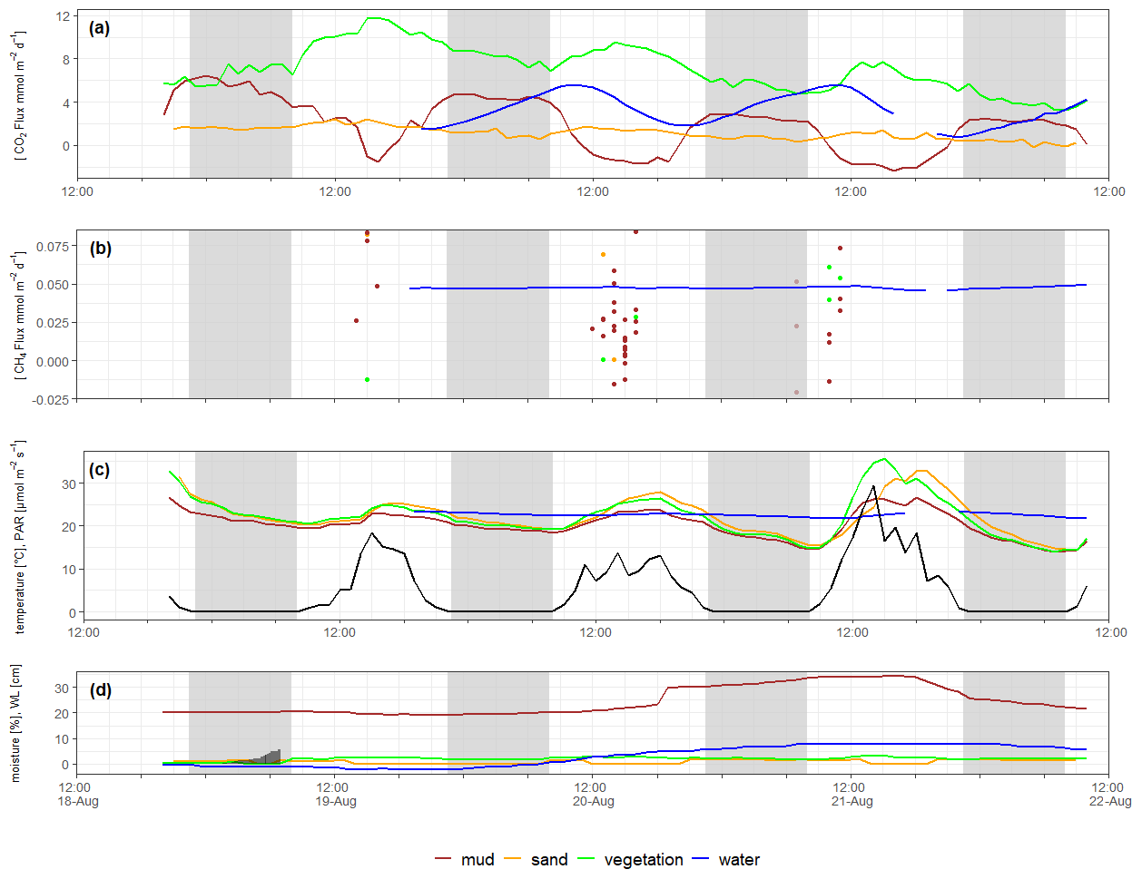
Figure 5 Time series of CO₂ flux (a), CH₄ flux (terrestrial CH₄ fluxes shown as dots since they were measured at different spots) (b), sediment and water temperature (c), and sediment moisture and water level (d). All data with hourly resolution. Black line in (c) shows light measured as PAR [µmol m⁻² s${}^{-\mathrm{1}}/\mathrm{2}$]. Grey-shaded areas indicate night. Grey bars in (d) indicate cumulative rain [mm] during the first night. Time is UTC. Please note that time series data were measured independently of spatial data in Table 2.

As a result of these diurnal patterns, fluxes were significantly higher during the day than during the night at the sandy and vegetated sites, while at the muddy site fluxes were higher at night than during daylight (Table 3). At the aquatic site, median values did not differ significantly between day and night.

We correlated the dry CO₂ flux with the measured potential drivers (Fig. S8). The CO₂ flux was weakly negatively correlated with sediment moisture and water level. Correlation with temperature or light (which were significantly linearly correlated, F test, p<0.05) including all data was not significant (F test, p>0.05), which is consistent with the different diurnal pattern observed at different sites. Furthermore, the temperature of the water was relatively constant – in contrast to the dry sites where diurnal temperature amplitudes of up to 20 °C were observed (Fig. 5c). If we correlate the CO₂ flux with temperature or light for each habitat type separately, we get a significant positive correlation at the sandy and vegetated sites, while the correlation is negative at the muddy and aquatic sites (Fig. S9, Table S2). A positive correlation with light was observed at the vegetated site, while the correlation was negative at the muddy site.

A linear mixed model with (log-transformed) temperature, light, water level, and sediment moisture as fixed factors and site as random factor explained 76 % of the variability. The most parsimonious model (based on the AIC) contained water level as the fixed factor and had a conditional R² of 0.75 (Table S3).

3.4 Comparison of spatial and temporal variability

We calculated coefficients of variation (CV) to make spatial and temporal variability comparable (Fig. 6). Consistent with our hypothesis, spatial variability of CH₄ fluxes had a higher CV compared to CO₂ in dry habitats. Also consistent with our hypothesis, temporal variability of the CO₂ flux had a higher CV than the CH₄ flux at the aquatic sites. The spatial variability of both gases was similar in aquatic habitats (CV = 0.5). At the dry sites (where we did not measure temporal changes in CH₄ flux) the temporal variability of the CO₂ flux also showed a high CV. If we want to judge the consequences of this result on upscaling, however, the absolute height of the fluxes as well as the relative areas of the different habitats need to be considered.

Table 3 Median (range) of temporal GHG fluxes at different sites (data from Fig. 5). Day and night separated by sunrise and sunset. Day and night data were significantly different for the dry sites but not for the aquatic sites (Wilcoxon test).

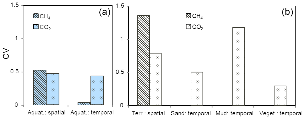
Figure 6 Coefficients of variation of spatial (calculated from Table 2) and temporal (calculated from Fig. 5) variability of CH₄ fluxes and CO₂ fluxes of aquatic sites (a) and dry sites (b) accordingly. Temporal variability of CH₄ fluxes from terrestrial sites was not calculated.

3.5 Upscaling

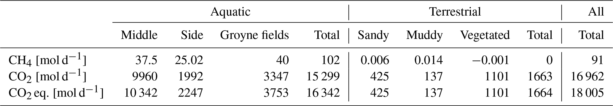
About 10 % of our study area was not covered by water (Table 2). Within the dry area, all three habitat types contributed similarly to the total area. If we apply an “optimal” approach considering spatial variability of CH₄ and both spatial and temporal variability of CO₂, our study reach emitted 91 mol CH₄ d⁻¹ and 16962 mol CO₂ d⁻¹ (Table 4). Thus, CH₄ contributed 5 % to total CO₂ eq. emissions. GHG emissions were dominated by the aquatic habitats, which contributed 91 % to the total emissions. CH₄ emissions from terrestrial habits can be neglected, while at the aquatic habitats they contributed about 6 % to the CO₂ eq. emissions.

Table 4 Total GHG emissions from the study reach quantified considering both spatial and temporal variability. For CO₂ emissions, we multiplied the median flux from the temporal data (Fig. 5) by habitat areas (Table 2). For aquatic CO₂ emissions, the temporal median flux at the side was also applied to the other aquatic habitats. For CH₄ emissions, we used the spatially different fluxes (Table 2). For CO₂ eq., the CH₄ emissions were converted to CO₂ eq. using a global warming potential of 28 and added to the CO₂ emissions.

4 Discussion

4.1 Spatial variability

Our results show considerable spatial variability of CH₄ fluxes from aquatic sites. This confirms earlier observations (Staniek, 2018) and can be explained by the fact that CH₄ is primarily produced in the sediment and, thus, depends on the spatial heterogeneity of the sediments. Although there was little CH₄ production also in the water, our incubation experiment confirms that the sediment was the dominant source of CH₄ in the Elbe. Sediment deposition in rivers is highly heterogeneous and depends on hydrodynamics (Henning and Hentschel, 2013). Fine material rich in organic matter preferably settles at low stream velocity, in our case in the groyne fields. Thus, our study confirms the hypothesis that the groyne fields are the major source of CH₄ in the Elbe (Bussmann et al., 2022). Consistent with observations of Matoušů et al. (2019) we did not observe ebullition, suggesting that ebullition is probably of minor importance in the Elbe. However, we can not exclude that ebullition might contribute to variability of CH₄ fluxes in dammed sections of the river, where high CH₄ concentrations were observed (Bussmann et al., 2022).

The data also revealed a significant difference between aquatic and terrestrial CH₄ fluxes (Wilcoxon test, p<0.05). CH₄ fluxes from dry sediments have rarely been measured, and there is still debate about their significance. A recent global survey indicates that these CH₄ fluxes probably cannot be neglected (Paranaíba et al., 2021). However, our results confirm previous observations that CH₄ fluxes from dry river sediments are rather small compared to CO₂ fluxes, both in terms of the carbon balance and the global warming effect (Koschorreck et al., 2022). It has been suggested that there might be local hot spots of CH₄ emissions (Marcé et al., 2019), but our measurements did not show any evidence for such hot spots.

We also observed considerable spatial variability in the CO₂ concentration in the water. Concentrations were lower in the groyne fields, most probably because of higher photosynthetic activity and higher plankton biomass (Pusch and Fischer, 2006). However, different CO₂ concentrations did not translate into spatial differences in CO₂ fluxes, because higher CO₂ concentrations were accompanied by lower gas transfer velocities. Higher gas transfer velocities at the side of the river were probably caused by higher turbulence generated from flow energy dissipation. This highlights the interacting role of both concentration and gas transfer velocity in shaping spatial patterns of GHG fluxes from rivers.

While spatial differences in concentrations have already been acknowledged (Bussmann et al., 2022) our study is, to our knowledge, the first to show small-scale spatial differences in gas transfer velocities in a river. Measuring k₆₀₀ in rivers is not an easy task, because tracer addition approaches, as typically used in small streams (Hope et al., 2001), cannot be applied. Eddy covariance measurements in rivers are possible (Huotari et al., 2013), but we consider the Elbe to be too small to exclude footprint contamination by the shore areas. Also, the eddy covariance technique integrates over larger areas and is thus not suited to addressing small-scale spatial variability. The floating chamber method is probably the only existing method that can be used in intermediate streams and rivers (Lorke et al., 2015). The spatial resolution of the method depends on the duration of the measurement, because the boat is drifting during the measurement. We minimized measuring time to about 2 min to optimize spatial resolution. Thus, at the measured flow velocity of 0.8 m s⁻¹, a typical flux measurement spanned a drift path of about 100 m, which might be the limit for the spatial resolution in the direction of the flow. Since we were drifting parallel to the shore, however, the method was well suited to distinguishing k₆₀₀ between the middle and side of the river. While higher k₆₀₀ values at the side of the river (where the groynes introduce turbulence) were expected, the high k₆₀₀ values in the groyne fields are somehow surprising. This indicates that factors such as bottom roughness and flow energy dissipation at the banks had a larger effect on turbulence and k than simply flow velocity (which was higher in the middle of the river). Wind was not an important factor controlling k₆₀₀ values in our study because wind speeds were low (Fig. S7). It can be expected that in larger and winding rivers with variable fetch, wind field heterogeneities further contribute to the spatial variability of k₆₀₀. It is reasonable to assume that spatially variable gas transfer velocities should also be considered for the exchange of other gases (e.g. Hg, Rn) or in stream metabolism calculations where k₆₀₀ is used to quantify oxygen exchange between the water and the atmosphere (Demars et al., 2015).

Compared to the aquatic sites, the CO₂ fluxes from terrestrial sites showed considerable inter-habitat variability. Higher CO₂ fluxes from darker (= more muddy) sites compared to sandy sites have been used to scale up CO₂ fluxes from dry river sediments using remote sensing (Mallast et al., 2020). They can be explained both by higher organic matter content of the muddy sediments as well as higher sediment moisture which favours microbial CO₂ production in the sediment (Keller et al., 2020). However, the trend observed here of decreasing CO₂ fluxes with increasing sediment moisture (Fig. 5) shows that wetter conditions do not necessarily result in higher fluxes. CO₂ fluxes from muddy sediments obviously result from a complex interplay between organic matter availability and moisture-dependent gas transport limitation (Keller et al., 2020).

The sediment in the proximity of terrestrial vegetation showed clearly elevated CO₂ fluxes, confirming earlier observations (Bolpagni et al., 2017; Koschorreck et al., 2022). Since we excluded plants from our chambers, these elevated CO₂ fluxes are probably caused by root respiration. It is well known that in soils, root respiration contributes about 50 % to soil respiration (Hanson et al., 2000). It is clear that at vegetated sites our CO₂ fluxes cannot be equated with net ecosystem exchange because the plants were excluded from our chambers. To fully assess the effect of terrestrial plants on river CO₂ fluxes, measurements using transparent chambers and considering light conditions as well as plant biomass determinations are necessary. The exclusion of plants from our measurements means that we systematically overestimate CO₂ fluxes from vegetated sites in the growing season. However, we argue that this bias might be small in our study when CO₂ uptake by the plants during the day was probably largely compensated by higher CO₂ fluxes due to plant respiration during the night.

For practical reasons it was not possible to perform measurements at all sites simultaneously (Table 1). Thus, our spatial data may contain also a temporal signal. Chamber measurements were made only for a few hours during the day. This probably did not affect our results for k₆₀₀ (because of rather constant wind and discharge conditions). CH₄ fluxes were also not affected, considering the very limited diurnal change of CH₄ concentration. Regarding CO₂ emissions, one may argue that the diurnal amplitude of the CO₂ concentration might differ between sites. For CO₂, differences between the middle of the river and the groyne fields can be expected to be lower at night because sediment-driven CO₂ production might increase CO₂ concentrations in the groyne fields during the night. This would further decrease the already low spatial variability of aquatic CO₂ emissions – supporting our conclusions. Thus, we think that our sampling design gave a realistic picture of spatial variability within our study reach.

Taken together, our results show that spatial differences were especially apparent for CH₄. The terrestrial habitats need to be considered for CO₂ emissions while they can probably be neglected for ecosystem-scale CH₄ emissions from the Elbe.

4.2 Temporal variability of CO₂ and CH₄

Our results confirm that the diurnal variability of CO_2,, which has been shown in streams (Attermeyer et al., 2021; Gómez-Gener et al., 2021) and in marine systems (Honkanen et al., 2021), can also be relevant in rivers. Interestingly, the shape of the diurnal curve of CO₂ emissions differed between habitats, showing that different regulatory mechanisms are at play.

At aquatic sites, biological fixation and mineralization of carbon led to sinusoidal diurnal pCO₂ variations, with a maximum in the morning and a minimum in the afternoon. This pattern was most likely driven by light, since the diurnal temperature amplitude in the water was below 1.5 °C.

The temporal pattern at the muddy site was also most likely driven by the interplay between microalgae primary production and respiration, but the shape of the diurnal CO₂ curve differed considerably. These data nicely demonstrate that the same regulatory mechanism (light-dependent balance of photosynthesis and respiration) may result in different diurnal patterns depending on the physical environments. In water, changes in biological activity are buffered by the dissolve inorganic carbon (DIC) pool in the water, resulting in gradual changes of CO₂ concentration during the day. At terrestrial sites, switching photosynthesis on and off changes the sediment from a CO₂ sink to a source and back again. Since microbial respiration depends on temperature and since temperature fluctuations in the sediment were quite large, it is somewhat surprising that we did not see a pronounced temperature signal in the CO₂ flux (as in Koschorreck et al., 2022). A possible explanation is that the CO₂ pool in the pore space buffers the effect of fluctuating respiration. Since the flux of CO₂ between the sediment and the atmosphere is driven by the concentration gradient, this results in rather constant CO₂ efflux during the night. During the day, this efflux is most probably blocked by photosynthetic uptake of CO₂ by benthic microalgae. In a laboratory study with marine sediments, a similar fast switching process between plateau-like CO₂ production in the dark and CO₂ uptake during the light was observed (Tang and Kristensen, 2007). Detailed investigations of benthic primary production on exposed marine sediments showed that both linear and plateau relationships were obtained between the fluorescence parameter (relative electron transport rate) and the community-level carbon-fixation rate (Migne et al., 2007). The reason for a “plateau behaviour” was the migration of some cells to greater depth in order to avoid too much light. Possible physiological explanations might be the existence of alternative electron sinks (e.g. the Mehler reaction or photorespiration) or limitation by Calvin cycle reactions.

At vegetated sites, the diurnal pattern was probably driven by diurnal fluctuating plant metabolism and root respiration. However, the diurnal CO₂ flux curve was not in phase with the light or temperature curve. This can be explained by a hysteresis effect caused by the transit time of CO₂ from the source of its formation (probably the plant roots) and the sediment surface (Koschorreck et al., 2022; Phillips et al., 2011).

From a previous study we know that rain events can reduce CO₂ emissions from sandy sites – most probably by blocking sediment pores (Koschorreck et al., 2022). We observed a small positive effect of the light rain on the first night only at the vegetated site. There was obviously too little rain to significantly affect sediment moisture and CO₂ fluxes either at the sandy site (were rain water just seeped or evaporated) or at the muddy site (where sediment was already wet).

Diurnal variability of CH₄ fluxes was observed in a study focusing on spatio-temporal variability of GHG fluxes in the Danube Delta (Canning et al., 2021). Elevated CH₄ fluxes from a floodplain lake and a channel were attributed to stratification and temporary mixing of the water column. In our case the water column was permanently mixed and diurnal variability was not an issue for CH₄ fluxes. Hydrodynamic conditions where rather constant during our measurements and wind speed was very low – suggesting that k₆₀₀ did not change much temporally. Furthermore, the literature suggests that in rivers, wind speed (which is potentially variable during the day) has a small effect on k compared to hydrodynamic parameters (which are rather stable on the timescale of days) (Huotari et al., 2013; Molodtsov et al., 2022). CH₄ is produced in deeper sediment layers and, thus, is not affected by light-driven changes of redox conditions at the very surface of the sediment. CH₄ consumption (oxidation) can occur either at the sediment surface or in the water column (Matoušů et al., 2019). A recent study, however, suggests that this process is not influenced by light and thus by daily variations (Broman et al., 2023). Even if CH₄ oxidation at the sediment surface were to be affected by phototrophic activity, this would not result in fluctuating fluxes at the water surface because these are buffered by the CH₄ pool in the water column.

Thus, we have confirmed our hypothesis that diurnal variability is relevant for CO₂ but not for CH₄. We also show that the shape of the diurnal CO₂ flux curve depends on the habitat. As already acknowledged in the literature, this has important implications for monitoring strategies and upscaling (Gómez-Gener et al., 2021).

4.3 Implications for measurement strategies and upscaling

Based on our results, the best monitoring strategy for our river reach should consider the spatial variability of CH₄ and both the spatial and temporal variability of CO₂. Applying this optimal approach to our data (Table 4) revealed the dominant role of CO₂ (due to low CH₄ fluxes) and aquatic habitats (due to their larger area).

It is evident that the exact quantification of habitat areas is crucial. Stream surface areas are typically estimated from empirical relations depending on stream order (Raymond et al., 2012) or remote sensing (Palmer and Ruhi, 2018). Estimating river width from annual mean discharge, according to Raymond et al. (2012), reveals a width of 183 m in our case. This is similar to the mean width of our reach of 200 m, which we obtain by dividing the water surface area (Table 2) by reach length (0.96 km). Although we found good agreement between measured widths and those calculated using the equation of Raymond et al. (2012), measured widths should always be used for field studies because of the large scatter in the regression and the logarithmic scale used. Thus, if river width is not explicitly measured, expected errors can become considerably larger than the standard error. These approaches, however, do not include dry sediment areas. In our case, 9 % of the total area was dry, which is somewhat lower than the 26 % estimated from remote sensing data during the extreme drought in 2018 (Mallast et al., 2020). During that drought, dry sediment areas showed clear longitudinal variability along the river depending on topography, ranging from 2 % to 40 % of the river area being dry. A straightforward strategy would be to determine dry areas for different discharge scenarios to derive a quantitative relation between dry area, water area, and discharge.

We used our dataset to simulate different monitoring approaches and compared them with the optimal approach (Fig. 7). Only sampling the river during the day at the side would result in about 50 % underestimation of the real GHG emissions – mostly because higher CO₂ fluxes during the night are not considered. Measuring in the middle of the river or even in all habitats during the day would only slightly improve the result. If both CO₂ and CH₄ fluxes were measured over a 24 h cycle only along the side of the river, we would slightly overestimate emissions because of high CH₄ fluxes along the side. The convenient approach of deploying only a CO₂ probe at the side of the river would result in about 7 % underestimation of total CO₂ eq. emissions from our study reach.

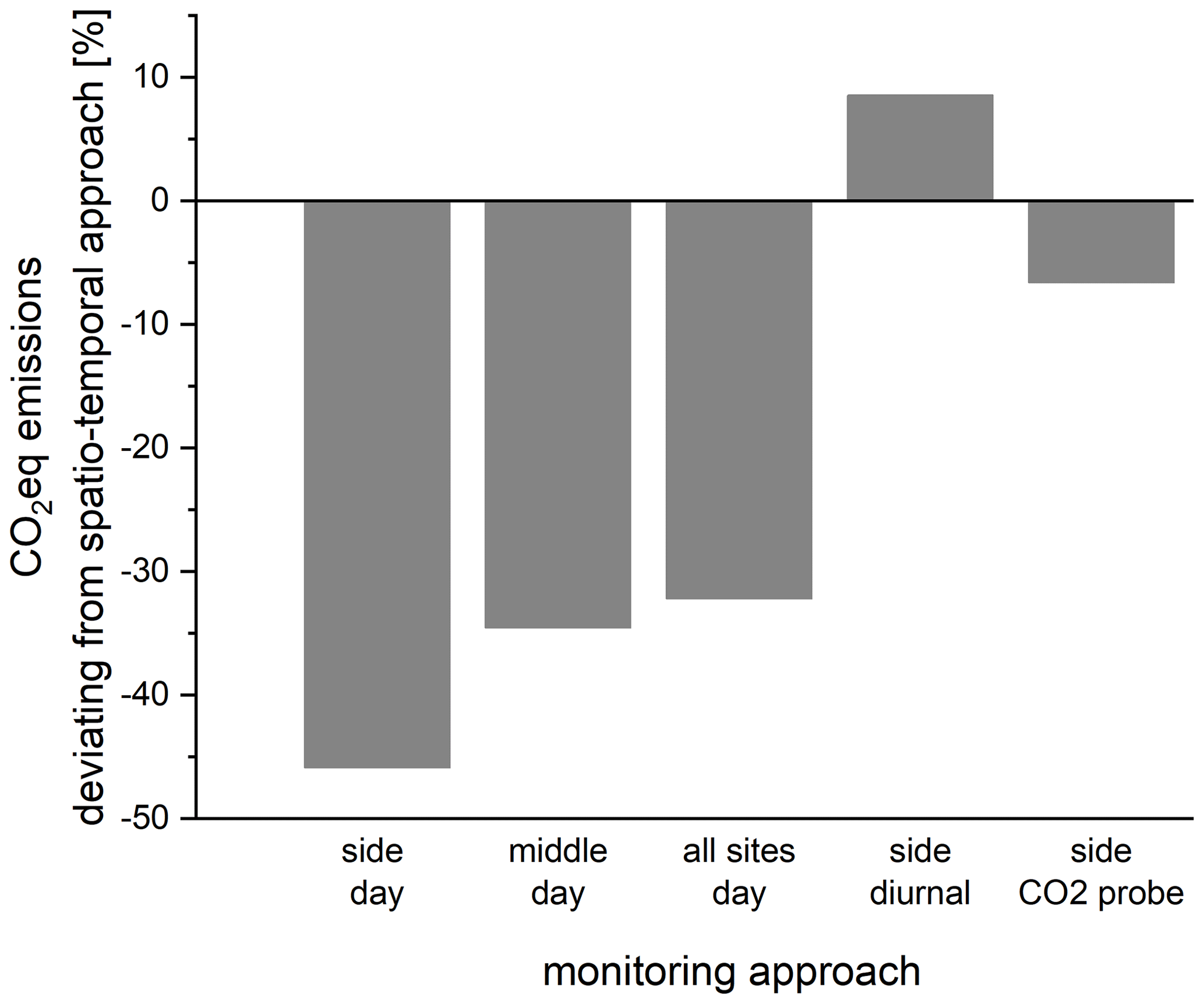
Figure 7 Deviation of total GHG emissions (CO₂ eq.) obtained by different monitoring approaches from optimal spatio-temporal approach (spatial variability of CH₄ and both spatial and temporal variability of CO₂ considered).

However, these considerations differ depending on the target gas. If we sample only during the day along the side of the river, for example, we would underestimate CO₂ emissions by about 50 % but overestimate CH₄ emissions by 100 % (Fig. S9).

Although our results reveal some general principles, they cannot be simply applied to other systems. For the design of a perfect monitoring strategy for a given river, the particular habitat types and diversity need to be considered. We can also expect that the role of spatial and temporal variability changes with the season, because habitat areas and regulatory factors such as temperature or day length change (Koschorreck et al., 2022). We would also expect that CH₄ variability needs to be re-assessed if ebullition becomes relevant (Maeck et al., 2014), especially in dammed river sections (Matoušů et al., 2019) or floodplain waters and under warm conditions (Barbosa et al., 2021). More natural river floodplain systems containing floodplain lakes are known to harbour extreme spatial variability with significant CH₄ fluxes (Maier et al., 2021), calling for a more sophisticated monitoring approach (Canning et al., 2021).

5 Conclusions

Although we only provide a snapshot case study at a German river, we can derive a number of conclusions relevant for the quantification of GHG emissions from large temperate rivers.

We show that short-term temporal variability is both relevant and complex. It is now evident from several studies that day and night measurements are necessary for determining realistic emission approaches. CO₂ probes are becoming more and more popular. Deploying them in numerous rivers will improve global riverine CO₂ emission estimates. Our results also show that diurnal patterns may differ between different habitat types. Light and temperature play different roles in shaping the temporal variability of CO₂ emissions in different habitats.

We also show that the spatial variability of CO₂ in different aquatic habitats can be considerable but it is not the only factor leading to spatially variable fluxes. k₆₀₀ also varied between habitats, and spatial variability of k₆₀₀ in rivers cannot be ignored. This point probably becomes less relevant in larger rivers where the side habitat area is small compared to total river area. There is a need for more studies addressing the spatial variability of k₆₀₀.

We also show principal differences between aquatic and terrestrial GHG emissions, both in terms of quantity and regulation. River sediments drying up at low discharge need to be considered at least for CO₂ budgets. However, when it comes to total GHG emissions, lower CH₄ fluxes compensate for higher CO₂ fluxes from dry sediments; this is a scenario already hypothesized for reservoir sediments (Marcé et al., 2019).

Finally, our data show that anthropogenic modification of the river (here: the construction of groynes) has the potential to alter GHG emissions significantly. In our case, the groyne fields nearly doubled the CH₄ emissions from the river.