the Creative Commons Attribution 4.0 License.
the Creative Commons Attribution 4.0 License.
 | 15 Apr 2024
Technical note: Flagging inconsistencies in flux tower data
Martin Jung
Jacob Nelson
Mirco Migliavacca
Tarek El-Madany
Dario Papale
Markus Reichstein
Sophia Walther
Thomas Wutzler
Global collections of synthesized flux tower data such as FLUXNET have accelerated scientific progress beyond the eddy covariance community. However, remaining data issues in FLUXNET data pose challenges for users, particularly for multi-site synthesis and modelling activities.
Here, we present complementary consistency flags (C2Fs) for flux tower data, which rely on multiple indications of inconsistency among variables, along with a methodology to detect discontinuities in time series. The C2F relates to carbon and energy fluxes, as well as to core meteorological variables, and consists of the following: (1) flags for daily data values, (2) flags for entire-site variables, and (3) flags at time stamps that mark large discontinuities in the time series. The flagging is primarily based on combining outlier scores from a set of predefined relationships among variables. The methodology to detect break points in the time series is based on a non-parametric test for the difference in distributions of model residuals.
Applying C2F to the FLUXNET 2015 dataset reveals the following: (1) among the considered variables, gross primary productivity and ecosystem respiration data were flagged most frequently, in particular during rain pulses under dry and hot conditions. This information is useful for modelling and analysing ecohydrological responses. (2) There are elevated flagging frequencies for radiation variables (shortwave, photosynthetically active, and net). This information can improve the interpretation and modelling of ecosystem fluxes with respect to issues in the driver. (3) The majority of long-term sites show temporal discontinuities in the time series of latent energy, net ecosystem exchange, and radiation variables. This should be useful for carefully assessing the results in terms of interannual variations in and trends of ecosystem fluxes.
The C2F methodology is flexible for customizing and allows for varying the desired strictness of consistency. We discuss the limitations of the approach that can present starting points for future developments.
- Article
(13823 KB) - Full-text XML
-
Supplement
(924 KB) - BibTeX
- EndNote


The eddy covariance (EC) technique is widely used to assess the carbon dioxide (CO2), water, energy, and other GHG fluxes between the surface and the atmosphere. Employed across major biomes globally, it counts thousands of stations distributed across all continents and often organized in regional networks (Baldocchi, 2020). Then, the FLUXNET initiative organized global data collections and synthesis datasets such as the Marconi collection (Falge et al., 2005), the LaThuile dataset, and the FLUXNET2015 (Pastorello et al., 2020), which have become the backbone for global ecosystem research (Baldocchi, 2020).
Flux tower measurements and associated data processing are complex and often subject to site-specific conceptual, technical, and logistic challenges. Principal investigators (PIs) of EC sites voluntarily provide their data to regional networks or directly to FLUXNET under a common data policy and standard format. The data include half-hourly or hourly biometeorological, environmental, and flux variables, all calculated and averaged by the PIs from the high-frequency raw meteorological and EC data. Before submission to the networks, the PIs generally apply a set of corrections (e.g. coordinate rotation, time lag compensation, and spectral corrections), specific quality checks and quality assessment (QA/QC) procedures (Metzger et al., 2018; Vitale et al., 2020), and site-specific data filters. This processing applied by single groups is not strongly standardized. Thus, there is a high level of heterogeneity among sites concerning the completeness and effectiveness of applied quality control routines, the detailed metadata of instrumentation and applied processing, and the availability of measured and reported variables.
The FLUXNET community developed a series of standardized tools for (1) reviewing critical metadata for the processing (e.g. site identifier, coordinates, reported time zone, and instrumentation height), (2) flagging meteorological data of questionable quality based on semi-automated visual checks of the relationships among different radiation variables (Pastorello et al., 2014), (3) filtering fluxes collected in low-turbulence periods where the assumptions of the technique are not met (the so-called u* filtering; Papale et al., 2006), (4) gap-filling of missing data (Reichstein et al., 2005; Papale et al., 2006), and (5) partitioning of net ecosystem exchange (NEE) into ecosystem respiration (RECO) and gross primary productivity (GPP) components (Reichstein et al., 2005; Lasslop et al., 2010) and uncertainty calculations (Pastorello et al., 2020). These tools are also organized into a set of routines (ONEFlux – https://github.com/Fluxnet/oneflux, last access: 8 April 2024) that have been used in the FLUXNET2015 collection and continental network releases (e.g. AmeriFlux FLUXNET product, ICOS Level-2 data, Drought2018, and WarmWinter2020 collections). The routinely provided QC information for flux tower data informs us primarily about the presence of an accepted measurement and the degree and quality of the gap-filling estimate, while potential issues in the underlying measurements may not be indicated.
Despite the effort to continuously develop and update standardized and common post-processing routines for FLUXNET, some measurement issues and inconsistencies between variables are not easily detected – data quality also relies on the initial procedures applied by the PIs. This includes, for example, potential discontinuities in the time series due to undocumented changes in instrumentation or processing, which have developed over the last years and decades. To reduce the effect of differences in data treatment and QC between sites, some of the more structured networks, such ICOS in Europe (Franz et al., 2018; Heiskanen et al., 2022) and NEON in the USA (Schimel et al., 2007), started to standardize the setup and methods (Franz et al., 2018; Rebmann et al., 2018) and the processing (Sabbatini et al., 2018) according to strict protocols, together with the collection of full and detailed metadata. This facilitates centralized processing from the raw data and reprocessing with more advanced methods as they become available (Vitale et al., 2020), taking into consideration all the changes in the measurement setup and ecosystem state. Developing standardized processing and QC that work robustly and reliably for all cases is very challenging as ecosystems, land surface, and (micro-)meteorological conditions can be very heterogeneous between sites. Thus, the standardized methods used are not perfect, and site-specific issues can persist. For example, the nighttime-based NEE partitioning method (Reichstein et al., 2005) might give unreliable GPP and RECO results when temperature is not the main driver of respiration.
The remaining issues and inconsistencies in FLUXNET data pose limitations for synthesis studies, particularly for process-based or machine-learning-based model calibration and evaluation. The degree to which model–data mismatches are due to model deficiencies or perhaps data issues, either in the fluxes or in the meteorological data used as model input, is typically hard to judge, especially by non-EC experts. This can limit progress in improving the modelling for certain aspects. For example, from the perspective of machine-learning-based flux modelling by the FLUXCOM approach (Jung et al., 2019, 2020), some unanswered example questions on the contribution of potential flux tower data issues include the following (Bodesheim et al., 2018; Tramontana et al., 2016): (1) can we predict the interannual variability of sensible heat flux much better than that of latent heat flux due to differential observational uncertainties? (2) To what extent is the low skill in predicting NEE interannual variability at the FLUXNET site level due to temporal discontinuities arising from changes in instrumentation and setup? (3) How much of the issue in relation to model drought effects in GPP is due to flux-partitioning problems? (4) Where is the optimal trade-off between data quantity and data quality used for training machine learning models? To progress on such questions, we need a complementary data consistency control that is applicable across the network's heterogeneous data conditions and core flux tower variables, following objective principles and allowing for varying the strictness of tolerated inconsistency.
Here, we address this challenge of providing complementary consistency flags (C2Fs) for FLUXNET data. This complements the quality control applied by PIs (or centralized regional networks like ICOS and NEON) and ONEFLUX as it is exclusively based on inconsistencies among measured variables according to a set of well-defined criteria. The degree of allowed inconsistency, a strictness parameter, has an interpretable basis and can be varied by the user. The underlying framework allows for extending and customizing the methodology as better knowledge or experience becomes available. Its objective principles facilitate full automatization and thus integration into processing pipelines for, for example, FLUXCOM or ONEFLUX. It delivers the following: (1) flags for daily data points, as well as flags for entire-site variables for ecosystem fluxes and core meteorological variables, and (2) times at which large discontinuities in the data occur and may indicate issues due to changes in the instrumentation, setup, or footprint. C2F is primarily intended to assist in network-wide synthesis studies, e.g. for analysing the robustness of results in relation to the inclusion of detected data inconsistencies.
The specific objectives of this paper are to introduce the C2F principles and methodology and to synthesize detected flux tower data inconsistencies for the widely used FLUXNET 2015 dataset. We illustrate and discuss the fact that patterns of detected flux tower data inconsistencies seem to be associated with issues which, while generally known in the eddy covariance community, have not been flagged systematically yet. We provide a critical assessment of the C2F methodology to assist potential users in interpreting the flags and to guide potential future developments.
2.1 FLUXNET dataset
The FLUXNET2015 dataset (Pastorello et al., 2020) is a collection of half-hourly meteorological and flux data measured at 212 sites and collected from multiple regional flux networks. The geographical location of the sites ranges from a latitude of 37.5° S to 79° N and covers all the main plant functional types. Compared to previous releases of flux observations, the FLUXNET2015 dataset includes several improvements, in particular to the data quality control protocols and the data-processing pipeline (Pastorello et al., 2020).
The complementary data consistency checks described here were developed and applied to daily data (temporal average) for the variables mentioned in Table 1. We keep only daily data points that are based on at least 80 % of measured data or that are gap-filled with high confidence (as defined in Pastorello et al., 2020). The C2F was then applied to only those data points.
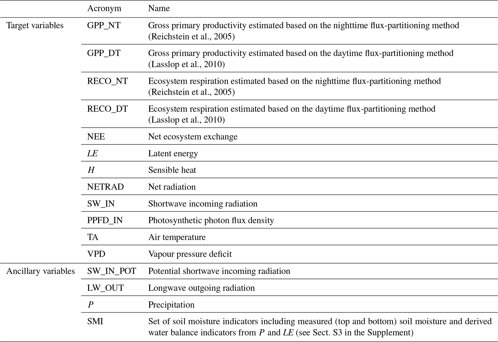
Table 1List of FLUXNET 2015 variables used in C2F. Target variables refer to variables for which flags are derived. Ancillary variables refer to additional variables used in C2F.
2.2 Flagging inconsistencies among variables
The approach described here is based primarily on multiple indications of inconsistency between variables for a given site. Its final output is a Boolean flag for every daily data point and target variable listed in Table 1, where TRUE indicates an inconsistency. Additionally, it reports a Boolean flag for entire-site variables, which is based mainly on between-site inconsistencies in relationships.
C2F is rooted in defining consistency constraints among variables (Fig. 1a) – these are the “brain” and determine where to look for inconsistencies. A constraint refers to an expected relationship of a target variable (e.g. SW_IN) with other variables (e.g. PPFD_IN) based on expert knowledge. We also use constraints where a target variable is modelled from a set of predictor variables using machine learning. Outliers derived from constraints indicate data inconsistencies. We distinguish between hard and soft constraints (Sect. 2.2.1) – flagging is enforced for outliers from a hard constraint, while for soft constraints, multiple indications of inconsistency are needed to cause flagging. The C2F procedure is based on three main consecutive steps (Fig. 1b): (1) outlier scores are calculated for each pre-defined constraint (Sect. 2.2.2) – this is the “heart” of C2F as it quantifies inconsistency; (2) all outlier scores available from different constraints for a target variable are combined to yield an inconsistency score per target variable, which considers multiple indications of inconsistency (Sect. 2.2.3); (3) flags are derived based on thresholding the inconsistency score according to a specified strictness parameter based on a consideration of outliers from individual hard constraints and further considerations (Sect. 2.2.4 and 2.2.5).
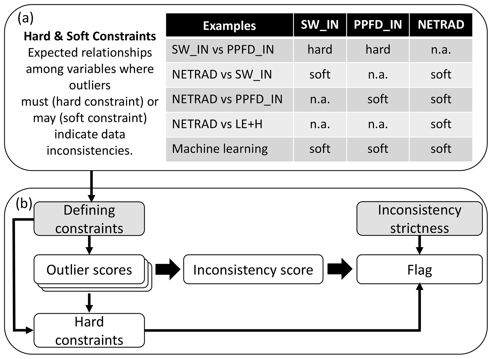
Figure 1Simplified overview of the C2F approach. (a) Definition of consistency constraints with assignments to target variables based on examples for radiation variables. (b) Flagging a target variable based on its inconsistency score, which considers multiple indications of inconsistency from several constraints and based on outliers from single hard constraints. The grey background indicates where a user can modify definitions and settings of C2F. Further steps of the flagging procedure were omitted for clarity here and are described in Sect. 2.2.4.
2.2.1 Constraints
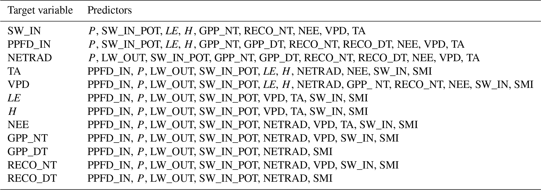
We use primarily bivariate constraints, i.e. linear relationships between two variables (e.g. SW_IN vs. PPFD_IN), and machine learning constraints, i.e. where a target variable is modelled from a set of independent predictor variables (Table 1). These deliver predictions to calculate residuals from the original data, which are then used to calculate outlier scores (Sect. 2.2.2). The linear models are based on robust regressions (RANSAC, random sample consensus; Fischler and Bolles, 1981). For the machine learning constraints, the predictions are based on a 3-fold cross-validation with random forests (Breimann, 2001) – the target-variable-specific predictors (Table 2) exclude variables that are already involved in other constraints for the same target variable to maximize independence among constraints. Soil moisture indicator variables were derived from measured precipitation and evapotranspiration (Sect. S3) and added as predictors to improve the predictability of fluxes under dry conditions. Gaps in predictor variables were imputed with missForest (Stekhoven and Bühlmann, 2011) to maximize data availability and applicability. Further implementation details are given in Sects. S3 and S4.
Each constraint is assigned to one or several target variables involved in the relationship. In the SW_IN vs. PPFD_IN example, the constraint is assigned to PPFD_IN and SW_IN because both are equally likely to be right or wrong for an outlier point. Likewise, the constraint LE + H vs. NETRAD is assigned to LE, H, and NETRAD. The constraint RECO_NIGHT vs. NEE_NIGHT is only assigned to RECO_NIGHT since it indicates primarily issues of the underlying flux-partitioning model rather than issues of measured NEE at night. Table S1 in the Supplement summarizes the assignment of constraints to target variables used here, while the methodology is flexible in adding, removing, or modifying constraints.
We introduced the distinction between soft and hard constraints to acknowledge that outliers from soft constraints do not always indicate data issues but could be explained otherwise. For example, outliers in the NETRAD vs. SW_IN relationship could also originate from sudden changes in the albedo, e.g. due to snow, harvest, or disturbance. Broadly speaking, hard constraints refer to physical relationships between variables where outliers reflect a problem in the data with high confidence. Soft constraints refer to relationships based on an underlying model where outliers could also occur due to violations of assumptions. For some of the soft constraints, we know that, for certain conditions, the relationship is not valid (e.g. NETRAD vs. SW_IN for negative net radiation) such that we can exclude those data from the beginning. Since flagging based on outliers from a soft constraint would imply the risk of false-positive flagging, we later combine multiple outlier indications from different and independent constraints (e.g. SW_IN vs. PPFD_IN, NETRAD vs. SW_IN) when calculating the inconsistency score for a target variable (here SW_IN, Sect. 2.2.3). In contrast to soft constraints, flagging is enforced for outlier data points for at least one of the variables assigned to a hard constraint (here SW_IN vs. PPFD_IN, Sect. 2.2.4) – this is where the distinction of hard vs. soft constraints matters for flagging in C2F.
Table 2Rationale for selected constraints. Median correlation refers to the median Pearson correlation coefficient calculated for each site when executing the constraints, i.e. based on daily data and with outliers removed (see Sect. 2.4 for details).
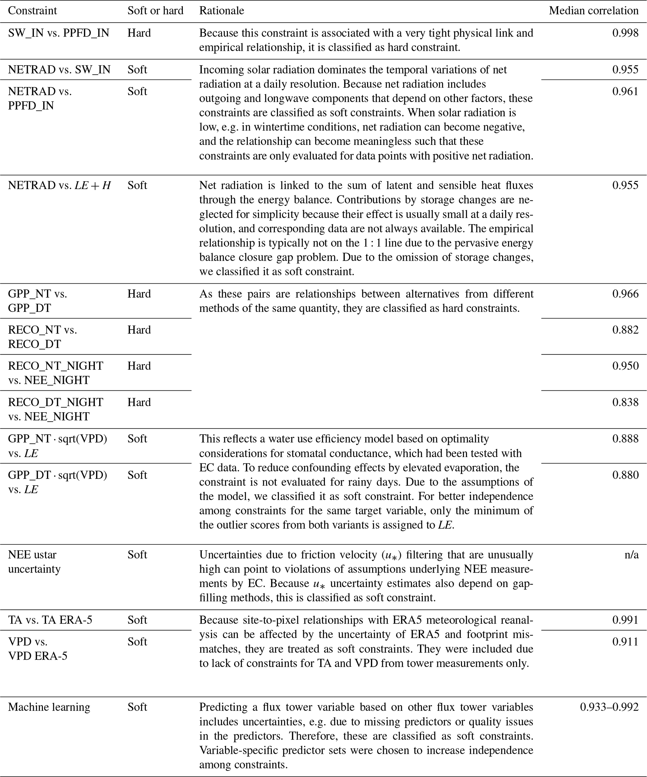
n/a – not applicable.
Table 3List of predictor variables used for different target variables. SMI stands for soil moisture indicator and denotes the set of measured (top and bottom) soil moisture (if available) and derived indicators CWDt, tCWD, and CWBt.
2.2.2 Outlier score for data points
Each constraint delivers a continuous outlier score, which quantifies for each data point i its deviation from the expected conceptual relationship. The calculation considers all daily data points available for a site in contrast to processing by year or moving windows. The outlier score is based on the residuals of the relationship for most constraints (). The predictions come from a robust linear regression model for bivariate constraints and from a cross-validated random forest model for machine-learning-based constraints (see Sects. S3 and S4 for details). Specifically, the outlier score measures the distance of a data point i to the closest quartile (P25, P75) in units of interquartile range (IQR). This corresponds to the widely used “boxplot rule”, while we take heteroscedasticity of residuals into account by estimating how the quartiles vary for every data point i depending on the magnitude of (Sect. S2).
The denominators refer to the interquartile range of the distribution of R, represented by two half distributions to account for asymmetric distributions (Schwertman et al., 2004) – the IQR for each side is estimated by 2 times the distance between the median and the first or third quartile.
This definition of the outlier score has several useful properties: (1) outlier scores from different constraints are independent of units, are comparable, and are therefore combinable among different constraints, which is an important prerequisite to calculate the inconsistency score later. Accordingly, this facilitates combining outlier scores from different constraints with different empirical strengths of the relationships because the outlier score for a constraint is relative to the spread of the residuals. (2) Biases due to heteroscedasticity are greatly reduced such that, for example, inconsistencies in small fluxes can be detected. (3) Its continuous nature allows us to consider different inconsistency strictness settings. (4) Its link to the widely used boxplot rule makes it easy to interpret and conceptually clear. The boxplot rule labels data points as outliers if they are 1.5 units of interquartile range (IQR) apart from the first or third quartiles; far outliers are often labelled when the distance exceeds 3 times the IQR. How many units of IQR (nIQR) should be chosen can be application dependent – it is essentially a strictness parameter that one might want to vary approximately between 1.5 and 3, corresponding to a gradient of “strict” consistency (retaining fewer data) to “loose” consistency (retaining more data). Thus, the parameter nIQR is the key consistency strictness parameter and is applied when calculating the inconsistency score (default value = 3 – can be varied by the user).
Figure 2 illustrates the outlier score for the machine learning constraint of GPP_NT for a dry site in the United States (US-Wkg). The machine learning model was trained with meteorological predictors and captures the flux patterns very well in general. However, it does not, for example, predict larger negative GPP values that are present in the FLUXNET2015 data. The residuals show a clear pattern of heteroscedasticity; i.e. residuals tend to be larger when GPP is larger. By taking this heteroscedasticity into account, we can identify the large negative GPP values in FLUXNET2015 as outliers, even when allowing for loose consistency with nIQR = 3. This is because the residuals are large relative to the expected narrow distribution of residuals for small GPP.
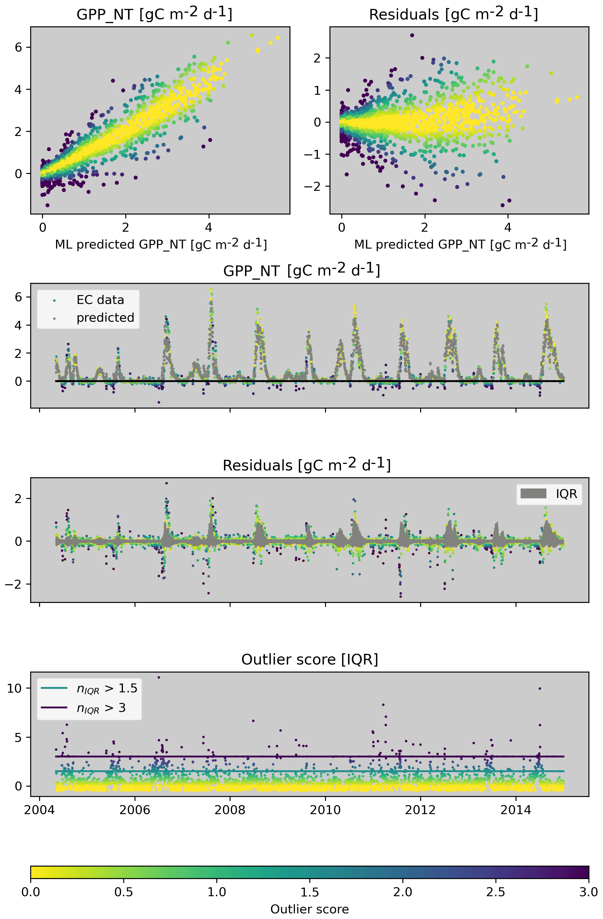
Figure 2Illustration of the derivation of the outlier score for a constraint. This example is for the machine learning constraint for GPP_NT for US-Wkg. Observed and predicted values are used to calculate residuals and how the distribution of residuals varies with the predicted value to account for heteroscedasticity. The outlier score measures the distance of the residuals to the quartiles in units of the interquartile range (nIQR). Please note that the colour scales with the outlier score in all the panels.
2.2.3 Inconsistency score of a data point
We first calculate the respective outlier scores for all constraints (Tables 2, S1). Then we combine them into an inconsistency score for each target variable, which takes multiple indications of inconsistency into account. To do so, we sort the vector of outlier scores assigned to a target variable for each data point i in descending order and normalize them by our consistency strictness parameter nIQR such that outliers would be indicated with outlier scores >1. The result we denote as , where the first value, denoted [1], is from the constraint with the largest outlier score; the second value corresponds to the second largest outlier score; and so on. The inconsistency score (I) is calculated when we have outlier scores from at least two constraints and is undefined otherwise:
In most cases, the inconsistency score is the second largest (normalized) outlier score from all available constraints for a target variable and data point. Conceptually, this refers to the situation where at least two constraints need to identify a data point as an outlier. Taking the maximum of the second largest, twice the third largest outlier score was chosen heuristically because occasionally three constraints show consistently elevated outlier scores, while the second largest does not exceed 1. For example, considering the choice of nIQR = 3, an inconsistent data point is flagged if two constraints show residuals outside the fence for nIQR = 3 or if three constraints show residuals outside the fence for nIQR = 1.5. If the inconsistency score is undefined, flagging is still possible if a hard constraint indicates an outlier (see Sect. 2.2.4).
The definition of the inconsistency score has several useful properties: (1) its calculation deals with the existing problem of heterogeneity in data availability (missing data) and associated gaps in the outlier scores because it can be readily computed for when we have two, three, or four outlier scores available per sample; i.e. not all constraints need to be available all the time. (2) As it considers multiple indications of inconsistency, it addresses the robustness problem. If there is a real problem in the data, it should be evident from several constraints. Individual soft constraints may indicate an outlier due to violations of underlying assumptions (i.e. false positives), while false-positive outlier indication for the same data point by different constraints is very unlikely if the constraints are independent. (3) It also addresses the variable attribution problem that we would have for most bivariate constraints when looking at a single constraint only. For example, we cannot attribute an outlier indicated in the PPFD_IN vs. SW_IN constraint to an issue in either of the variables. Instead, the inconsistency scores for the two variables consider all available constraints and thus provide an indication as to which variable is more likely to show a data issue.
We will illustrate this by means of an example of deriving the inconsistency score of SW_IN for a site in France (FR-LBr, Fig. 3). Figure 3 shows the three constraints available for SW_IN where the respective outlier scores scale with the colour: the bivariate relationships with PPFD_IN and with NETRAD, as well as the machine-learning-based constraint for SW_IN. In the scatter plots, we see two major patterns of inconsistency: (1) SW_IN scales differently with PPFD_IN for a subset of the data, and (2) all three constraints indicate an issue related to some values of zero for SW_IN. In the time series plots for SW_IN, we see that the first pattern of inconsistency between SW_IN and PPFD_IN occurs for a long consecutive period in 1997 and that the second pattern occurs in 2002, where SW_IN is constant at zero. The inconsistency score for SW_IN shows the latter issue accordingly since it is present in multiple constraints, while it shows no major issue for SW_IN in 1997, where there was an inconsistency with PPFD_IN only.
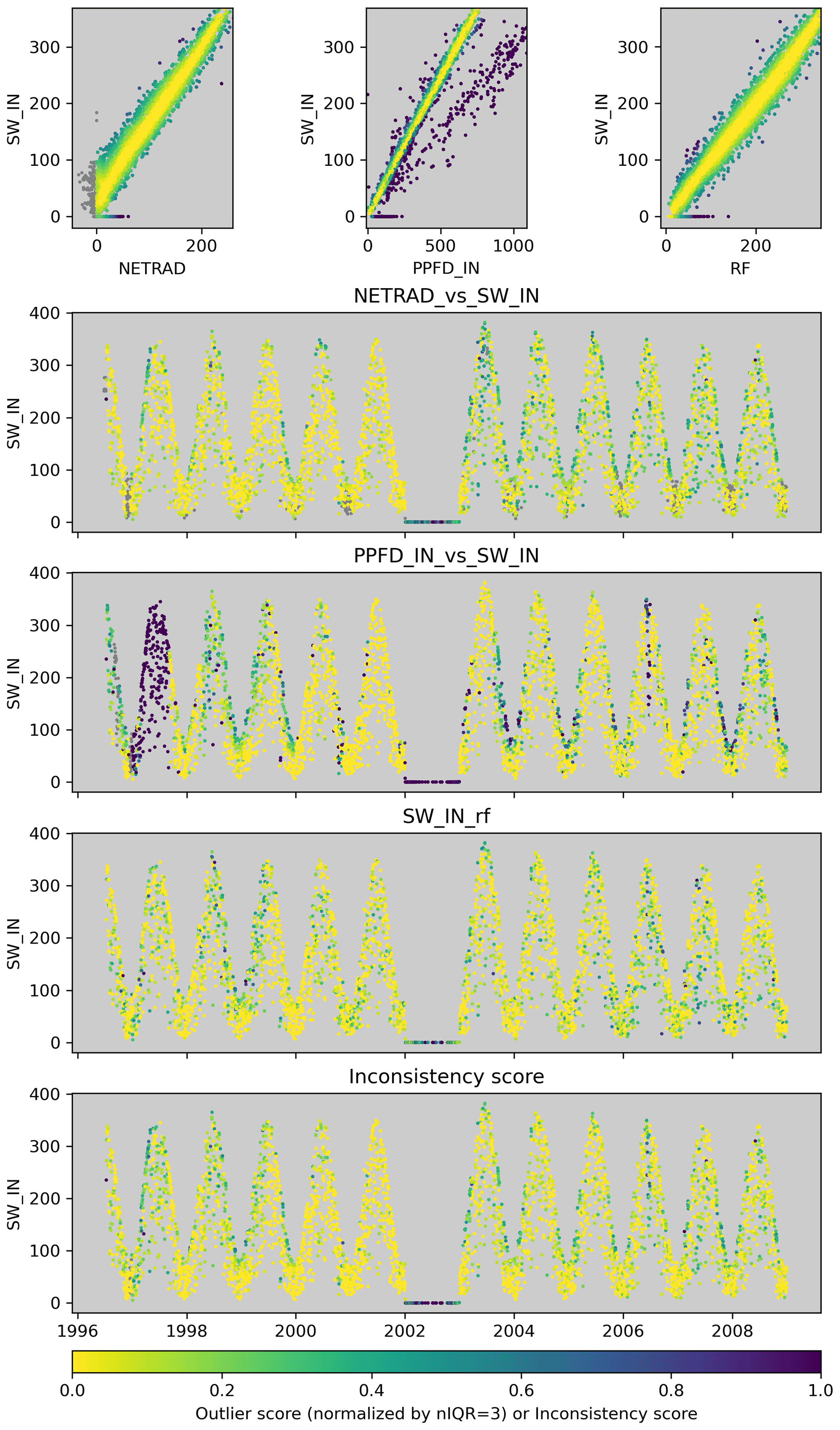
Figure 3Illustration of the derivation of the inconsistency score for a variable, here SW_IN for the site FR-LBr, based on outlier scores of different constraints. The colour scales with the outlier or inconsistency score in the same way across panels.
2.2.4 Flagging data points
The first step of flagging data points for a target variable is based on thresholding the corresponding inconsistency score at >1. Please note that this corresponds to the specified nIQR threshold, which was used to normalize the outlier scores for the computation of the inconsistency score (Sect. 2.2.3). In the second step, we iterate the procedures outlined below.
Table 4Predefined dependencies for flag propagation. Arrows indicate the direction of flag propagation.
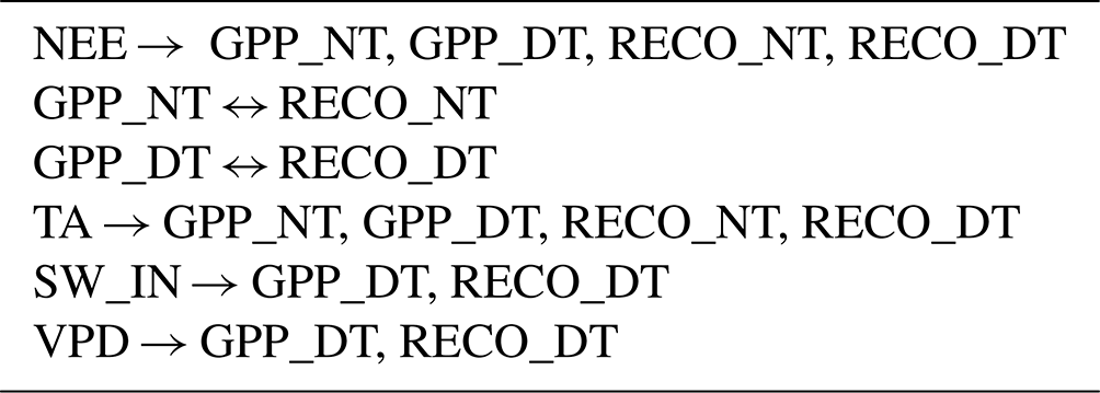
We propagate flagged data points to dependent variables (e.g. SW_IN is used to calculate GPP_DT during flux partitioning; see Table 4 for considered dependencies).
If two flagged data points are less than a few days apart (default = 4 d), we additionally flag these data points in between. This is done because data issues often appear in sequence, e.g. due to instrumentation issues or moving-window processing of the flux partitioning, while the inconsistency score may not always exceed 1.
If hard constraints indicated an outlier data point but none of the target variables assigned to this hard constraint were flagged yet, we force flagging for at least one of the associated variables. Which variable(s) gets flagged is determined by an attribution scheme that considers primarily the inconsistency scores of the variables associated with the hard constraint (Sect. S6). Forcing flagging for hard constraints (e.g. PPFD_IN vs. SW_IN) is done because we assume that there must be a data issue in at least one variable involved if an outlier is identified by this constraint, according to our definition of hard constraints (Sect. 2.2.1).
Turing back to our previous SW_IN example for the site in France, we see that the flagging has correctly flagged the PPFD_IN values in 1997 and flagged the SW_IN values in 2002 (Fig. 4). The SW_IN flag is propagated to GPP_DT, which shows the same problem as SW_IN in 2002.
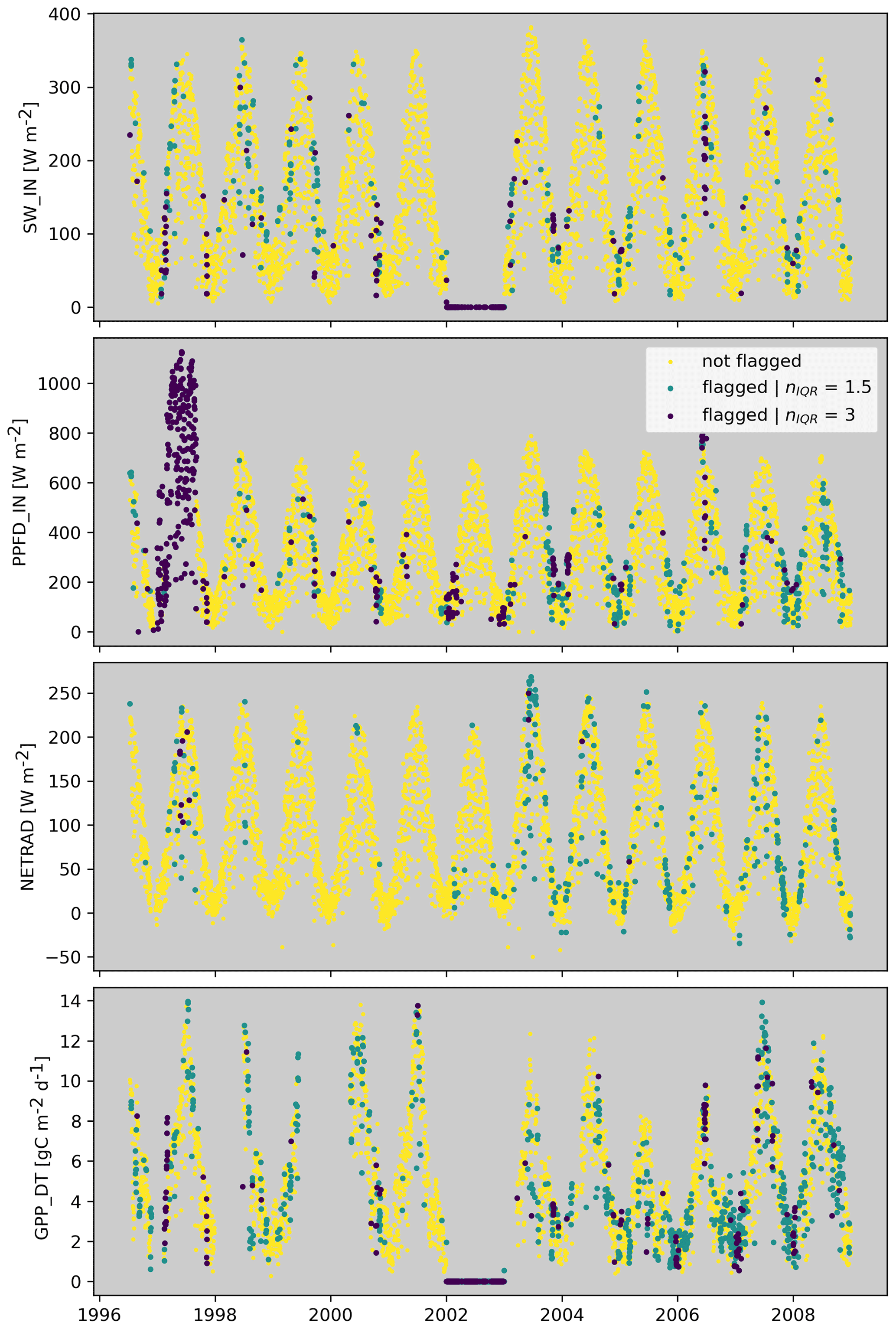
Figure 4Derived flags for SW_IN, PPFD_IN, NETRAD, and GPP_DT for FR-LBr for a strict consistency setting (nIQR = 1.5) and a loose consistency setting (nIQR = 3).
To further illustrate how multiple indications of inconsistency, as well as outliers from hard constraints, shape the flagging of carbon fluxes, we look again at the dry site from the US (Fig. 5). The flagged data points due to the inconsistency score (red points) are dominated by negative GPP_NT values. Many of those also correspond to outliers of the GPP_NT vs. GPP_DT constraint (blue stripes). For RECO_NT, we see that flagged values are dominated by outliers of the relationship between nighttime RECO_NT and nighttime NEE (hard constraint, magenta stripes). These data points occur predominately in the dry season, indicating issues in the nighttime-based flux-partitioning method (Reichstein et al., 2005). These data points, often associated with negative GPP_NT and elevated NEE, are often flagged independently for GPP_NT based on the inconsistency score. The propagation ensures that flags are finally consistent and identical for GPP_NT and RECO_NT, as well for GPP_DT and RECO_DT. Please note that hardly any data were flagged for NEE, indicating that data issues in GPP and RECO are likely dominated by flux-partitioning uncertainties rather than NEE measurement issues. The examples above illustrate that we can diagnose which constraints have contributed to or caused flagging by inspecting intermediate diagnostics of C2F, which might be interesting for eddy covariance experts to infer reasons for potential issues in the data.
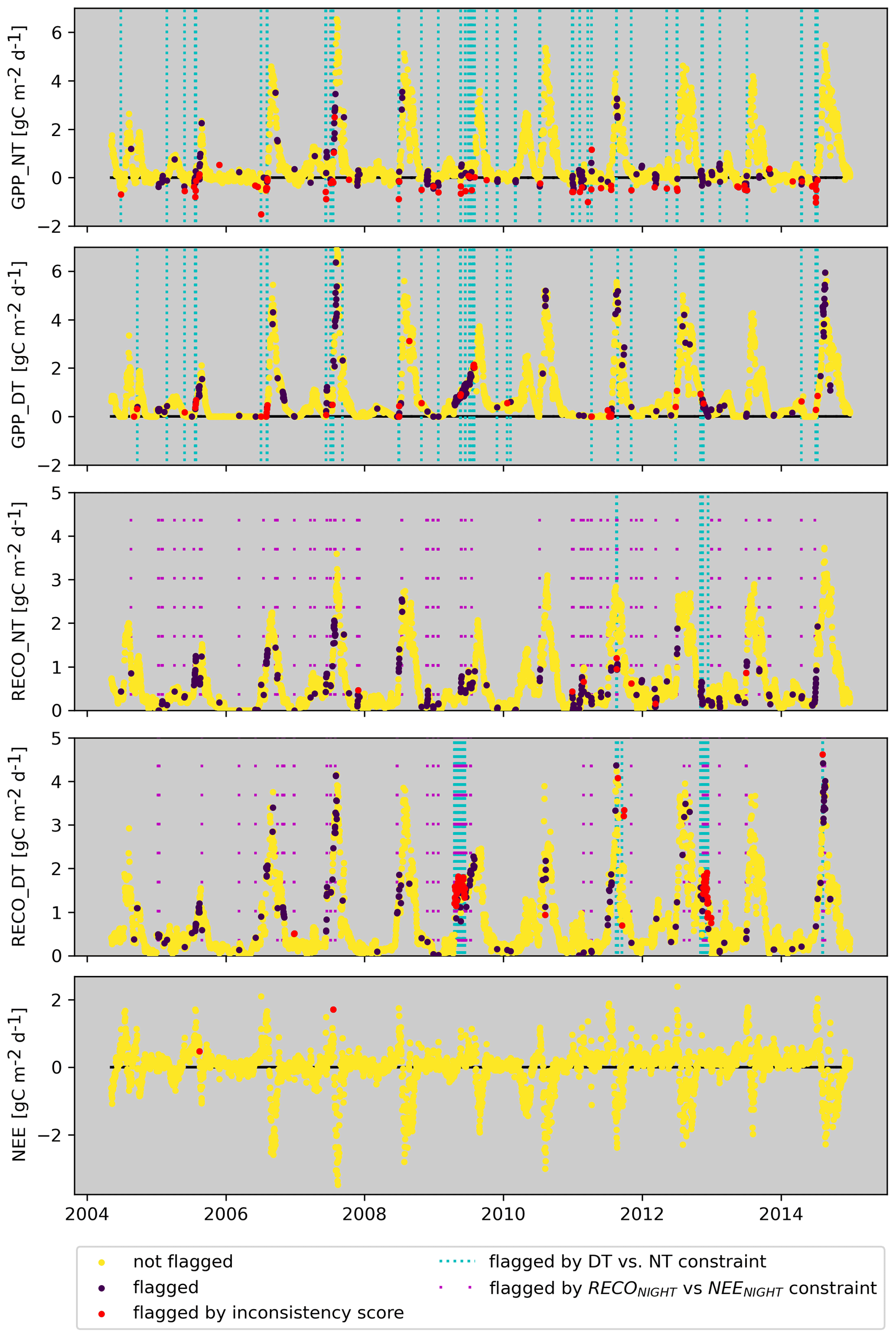
Figure 5Illustration for flagging GPP and RECO values from the nighttime and the daytime partitioning method for US-Wkg. The flagging is based on default values (nIQR = 3).
2.2.5 Flagging entire variables
So far, we have aimed at flagging inconsistent data points for a target variable within a site, given the information available for that site. Now we aim to identify if an entire-site variable time series, measured at one site, behaves unexpectedly and should perhaps be flagged. If, for example, a variable were to be in a wrong unit, the regression approaches used in the within-site inconsistency detection will not catch it, while, for example, the slope of the regression will emerge as unusual compared to the distribution of slopes from the same constraint available across sites. In a similar notion, if the relationship between two variables for a constraint is unusually weak for a site, the within-site processing will not catch this because it looks only for outliers, given the distribution of residuals within the site.
The constraints for flagging entire variables are based on the following: (1) the performance of the relationship from the machine learning constraints, (2) parameters of the linear model of the bivariate constraints in combination with its performance (see Fig. 6 for an illustration), (3) the fraction of flagged values for a variable from the within-site processing, and (4) a metric related to the NEE u* uncertainty per site as diagnosed by the within-site processing (only used for NEE; see Sect. S5). Because we add the fraction of flagged values per site as a between-site variable constraint, the number of between-site constraints per variable is one more than for the within-site processing (see Table S1). The above-mentioned diagnostics are converted into outlier scores considering the distribution across sites (see Sect. S7). The calculation of the inconsistency score per site variable and following flagging of site variables follows the methodology described for the within-site processing, except that we do not apply the consecutiveness rule in the flagging procedure as it is meaningless here.
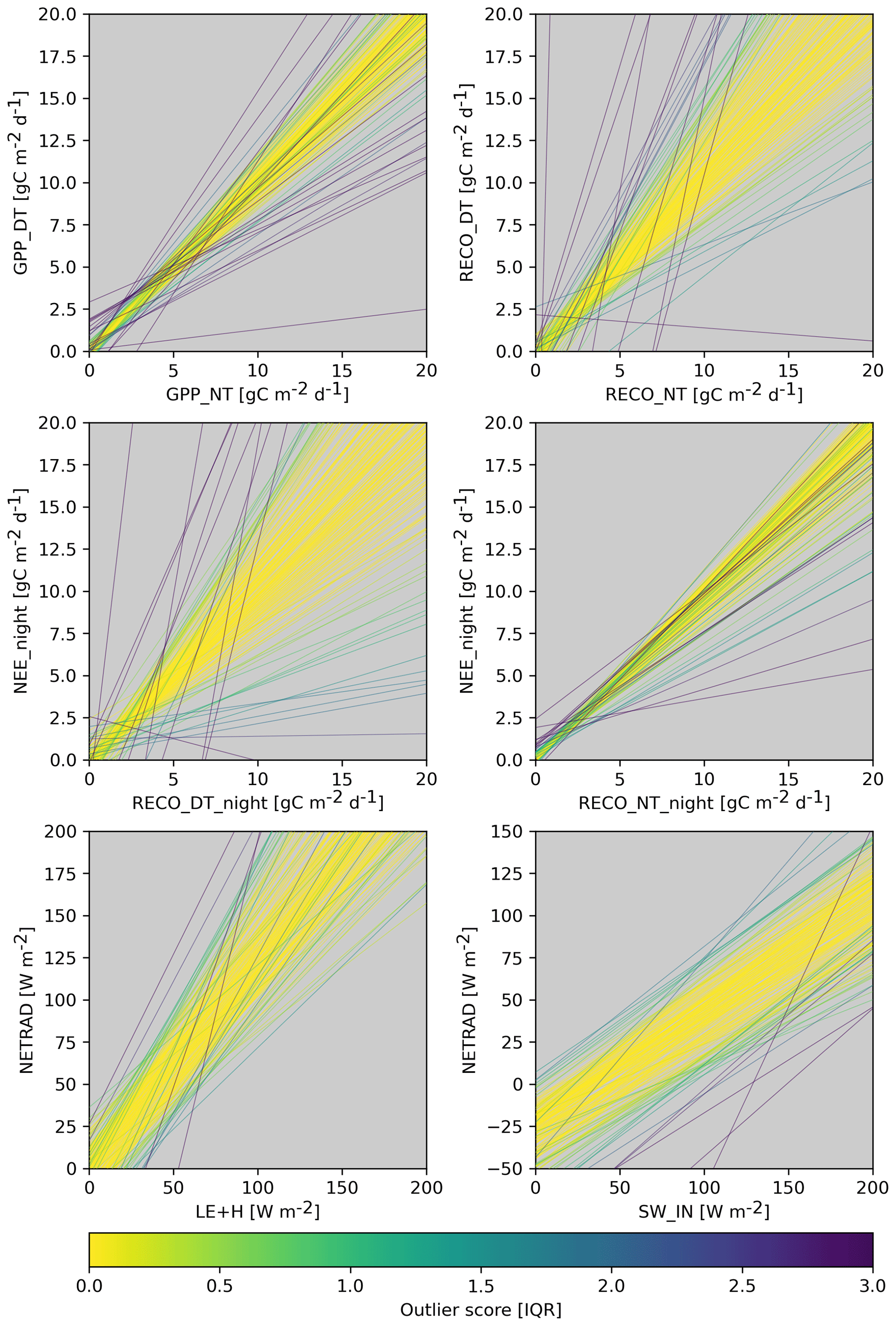
Figure 6Estimated regression lines for each site for some bivariate constraints. Each line corresponds to a site, and colours correspond to the derived outlier score for the specific constraint.
2.3 Identifying temporal discontinuities
Here, we aim to identify systematic changes in the distribution of flux tower data within a time series that could point to data artefacts, e.g. due to instrumentation, setup, or data-processing method changes. Temporal discontinuities are assessed per target variable and site. In addition to removing gaps, as described in Sect. 2.1, we also remove flagged data points for the target variable. The basic principle is to move from the beginning of a time series to the end. At each time step, we assess the difference in the distribution between the data before the current time step and the distribution after the current time step. This yields a new time series of the test statistic for the difference in distributions for which we seek the maximum (Fig. 7). We use a non-parametric test for the equality of two distributions (Eq. 3) based on their energy distance (Szekely and Rizzo, 2004) – intuitively, energy distance can be understood as the amount of work necessary to transform one distribution into the other.
In the above equation, n1 and n2 denote sample sizes for the temporal segments X and Y, respectively, and denotes Euclidean distance. The term in the brackets equals the energy distance between the distributions of X and Y, which measures 2 times the mean distance among samples between X and Y minus the mean distance among samples within X and within Y.
The change in distribution is assessed based on residuals of two machine learning models for the target variable and site (see Sect. S8 for details). The first model uses meteorological conditions as input, while the second model uses only seasonal information as input. The residuals of both models are normalized to account for heteroscedasticity. The test statistic for the difference in distribution is calculated based on distances in two-dimensional space, where the two dimensions correspond to the time series of the normalized residuals of the two models. The rationale for this approach is discussed in Sect. 4.1.2.
The breakpoint detection is setup as a recursive partitioning where the time series is iteratively split into segments. For example, we first run the breakpoint detection on the full time series. Then the time series is split into two segments according to where we found the largest difference in distributions. Then the breakpoint detection is run for both segments again. This procedure continues until no sufficient data are in the segments (default = 100 data points). For every split, we calculate and store a break severity metric that is used to calculate a corresponding outlier score (Sect. S8).
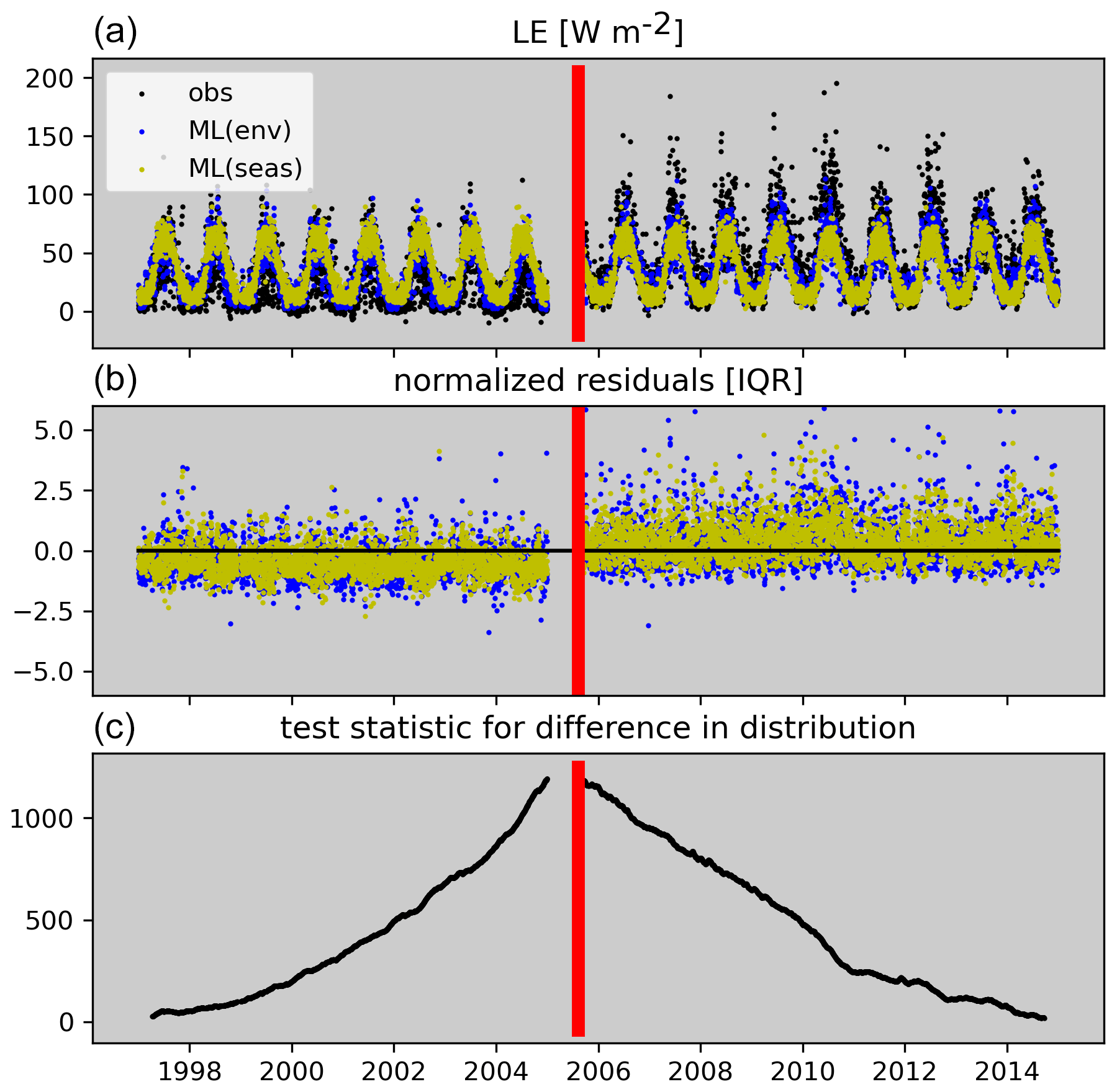
Figure 7Illustration of the break point detection for CH-Dav. Panel (a) shows the observed time series of daily LE and model predictions. Panel (b) shows the normalized residuals that are passed to the breakpoint detection. Panel (c) shows the estimated test statistic for the difference in distributions, which is maximized at the red bar, which denotes the detected break.
3.1 Patterns of flagged data
Running the C2F algorithm across all sites in FLUXNET 2015, we find the most flagging for GPP and RECO, followed by SW_IN, NETRAD, and LE, and comparatively few rejections for H, NEE, TA, and VPD (Fig. 8). These differences in the fraction of flagged values do not entirely reflect a gradient of data inconsistency but can also be influenced by the number and quality of constraints available for the different variables (for discussion, see Sect. 4.1.1). Increasing the consistency strictness from more loose (nIQR = 3) to more strict (nIQR = 1.5) can cause more than a doubling of flagging. For GPP and RECO, the fraction of flagged data exceeds 20 % for strict (nIQR = 1.5) consistency and is below 10 % for loose (nIQR = 3) consistency across the full data set, while there is a tendency toward slightly more frequent flagging for the daytime-based estimates compared to the nighttime-based estimates. There is substantial variability in the fraction of flagged data between sites (Fig. 9, top panel).
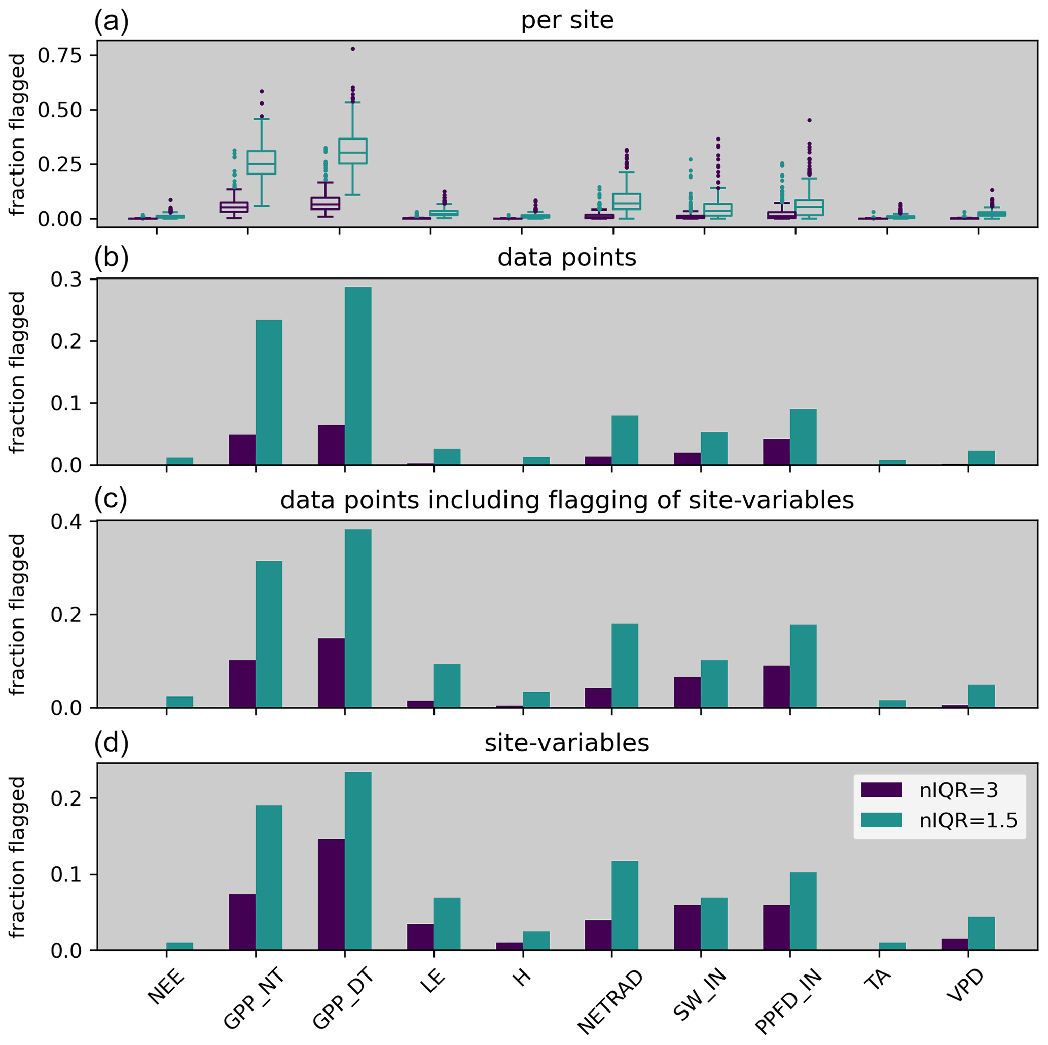
Figure 8Summary of the fraction of flagged data for FLUXNET 2015 for loose (niqr = 3) and strict (niqr = 1.5) consistency. Panel (a) shows the distribution across sites. Panel (b) shows the fraction of flagged data points across the full FLUXNET 2015 data set while not considering when an entire-site variable was flagged – these data points are included in (c). Panel (d) shows the fraction of sites for which an entire variable was flagged.
We take a closer look at GPP and RECO flagging in order to better understand the pattern of frequent flagging. Figure 9 shows a systematic pattern of flagged GPP and RECO values when temperatures are high and GPP is low for both nighttime- and daytime-based partitioning. These conditions correspond typically to very dry conditions, where the assumptions of the NEE flux-partitioning methods are more frequently violated: ecosystem respiration is less controlled by temperature, and GPP is less limited by light. Visual inspection of the time series (e.g. Fig. 5) suggested particular flux-partitioning issues during respiration rain pulses, where, for example, GPP_NT is often systematically negative, while NEE is elevated. We found a systematic pattern of strongly elevated flagging frequency during and after rain when temperatures are high (>15 °C) and GPP is low (Fig. 9). This illustrates methodological limitations of the flux-partitioning methods in dealing with rapid changes in ecosystem responses due to the used moving-window approach to estimate parameters during flux-partitioning processing. To verify that the systematic patterns found for flagged GPP and RECO values under high temperatures and low GPP conditions are not an artefact of the method, we compare them with the patterns for LE and H, where we essentially see no systematic patterns in the relative frequency of flagged values, along with a 1-order-of-magnitude-smaller fraction being flagged.
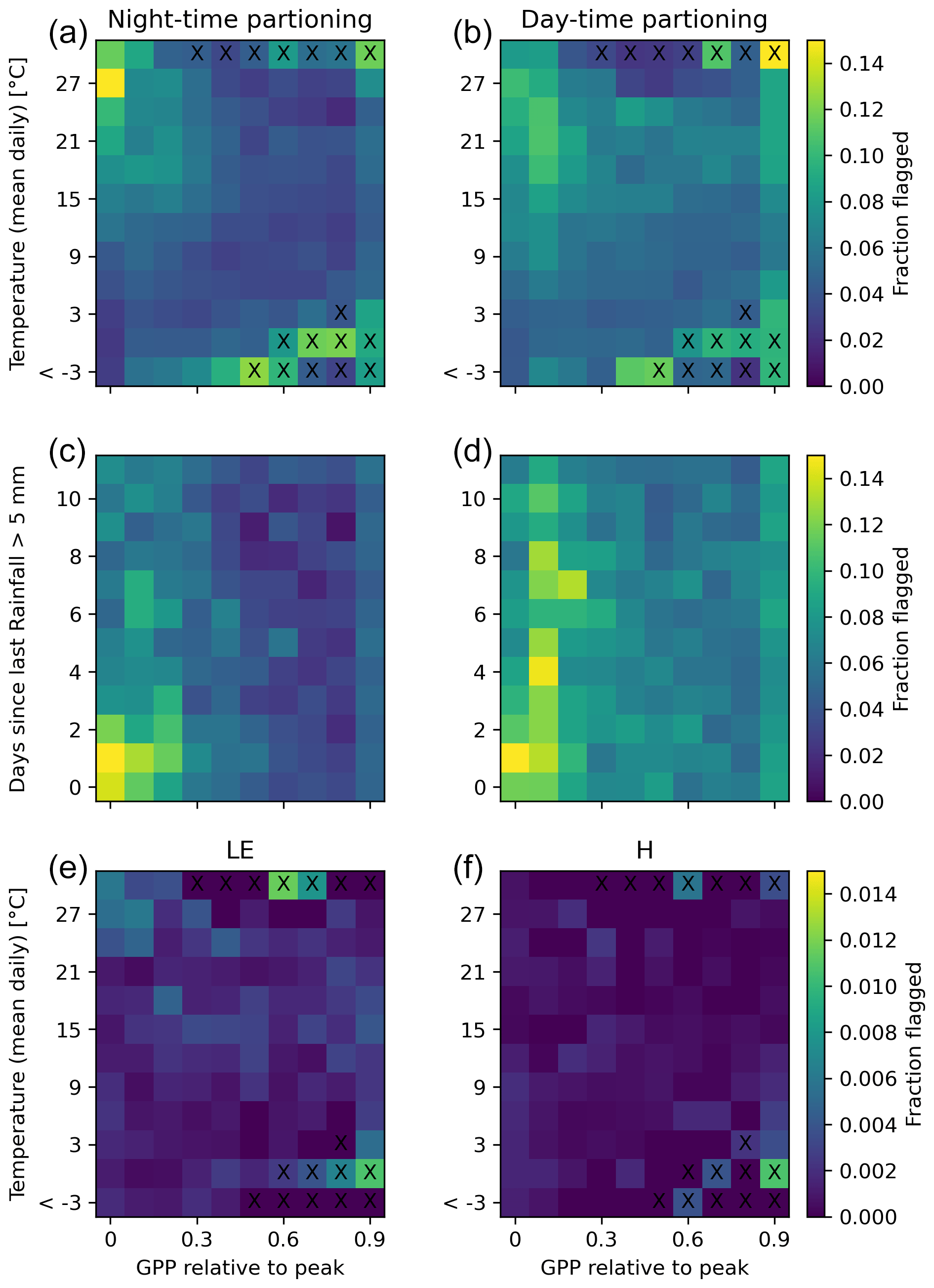
Figure 9Relative flagging frequency for nighttime and daytime flux partitioning (GPP, RECO, a, b), latent energy (LE), and sensible heat (H, e, f) as a function of daily temperature and relative GPP. Panels (c) and (d) show flagging patterns for GPP and RECO as a function of days since last major rainfall event, where only data with daily temperatures >15 °C were included. Crosses indicate very rare occasions (<0.05 % of data points in the bin).
We assess whether the flagging of all the GPP or RECO variables for the sites also follows a systematic pattern, and we find that there is indeed some prevalence of flagging for sites with low mean annual precipitation and with high mean annual temperatures (Fig. 10). A similar pattern is not clearly evident for other variables, except for the flagging for NETRAD at very cold sites. The prevalence of flagging GPP and RECO variables for very cold sites might be related to issues caused by polar days and polar nights, i.e. when, during the growing season, no or hardly any nighttime measurements are available to constrain the respiration response to temperature.
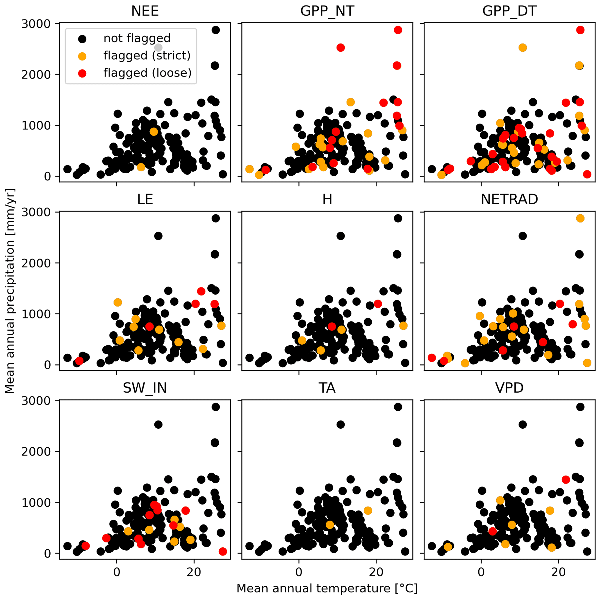
Figure 10Flagged site variables in mean temperature and precipitation space. Each dot corresponds to a site.
We now assess to what extent flagging might be systematic for extreme conditions recorded in the time series of the sites. We chose to look at cold, normal, and hot conditions because temperature extremes are a common topic of interest and because the temperature variable showed the fewest data inconsistency issues. The boundaries for the temperature extremes were chosen according to the boxplot rule for the distribution of measured daily temperatures at each site, with a threshold of 1.5 units of interquartile range in terms of distance from the median. Overall, we see no evidence that the C2F would be flagging a high fraction of data points related to extreme temperatures (see y-axis values in Fig. 11). However, for some variables, we see a larger fraction of flagged values for extreme temperatures compared to normal. Relatively more frequent flagging for GPP under hot conditions likely reflects primarily real data issues related to violations of flux partitioning under drought conditions, as outlined above. NETRAD also shows elevated flagging rates at high temperatures, and H shows elevated flagging rates for cold temperatures, while the vast majority of data are still retained. For TA, flagging rates are increased under cold and hot conditions compared to normal but are small on an absolute level. Overall, we conclude that there are some indications of more frequent flagging under extreme conditions. At the same time, the percentages still remain small, suggesting that the C2F procedure is generally robust in relation to and not very biased at extreme conditions. The slight tendency toward elevated flagging percentages at extreme temperatures might be related to limitations in estimating heteroscedasticity in very data-sparse conditions (for discussion, see Sect. 4.1.1).
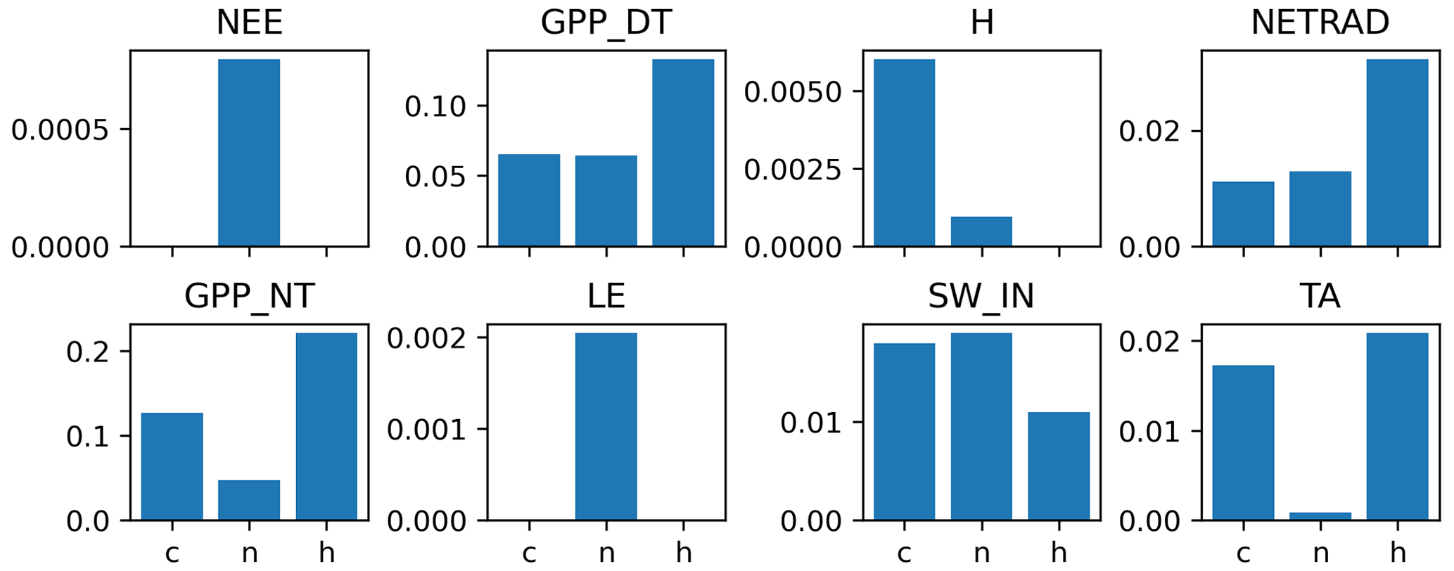
Figure 11Relative rejection frequency for cold, normal, and hot temperatures corresponding to the loose-consistency criterion (nIQR = 3). The stratification in temperature classes is based on the boxplot rule applied separately for each site with nIQR = 1.5.
3.2 Patterns of large temporal discontinuities
Figure 12 illustrates for some sites that large discontinuities in the time series are detected for ecosystem fluxes and meteorological variables, which often coincide with documented changes in instrumentation (BADMs) or changes in the ecosystem. Changes in instrumentation can explain detected discontinuities, e.g. at IT-SRo in 2007–2008 for NEE and LE, at CH-Dav in 2005 for NEE and LE, at BE-Lon in 2007 and 2012 for NEE, at CA-TP1 in 2008 for NEE, at NL-Loo in 2004 for NETRAD, at AU-Tum in 2008 for NETRAD, and for IT-Col in 2005 for SW_IN. Changes in the ecosystem have likely caused detected discontinuities at DE-Tha for NEE in 2002 (thinning) and at FR-Pue for NEE in 2005 (thinning). No discontinuity was detected for the long NEE time series at DE-Hai, indicating that the method is quite robust in relation to (real) interannual variability caused by weather. The reason for the many discontinuities of NEE at BE-Lon is likely that it is a site with crop rotation, while some detected discontinuities coincide with changes in instrumentation. Likewise, CA-TP1 is a growing forest plantation established in 2002, with an associated strong trend in ecosystem structure which could explain the detection in 2008, while this also coincides with changes in instrumentation. Time series patterns suggest that detected discontinuities at FI-Sod for H and at IT-BCi for TA are also likely due to changes in instrumentation, while those were not reported in the BADMs.
There are several instances where changes in instrumentation are not associated with the detection of a temporal discontinuity (e.g. FI-Sod in 2003), and there are likewise several detected discontinuities, which we cannot associate with documented changes in instrumentation or ecosystem properties. These considerations highlight the importance of correct and complete metadata on instrumentation and ecosystem changes for interpreting time series of flux tower measurements and detected discontinuities.
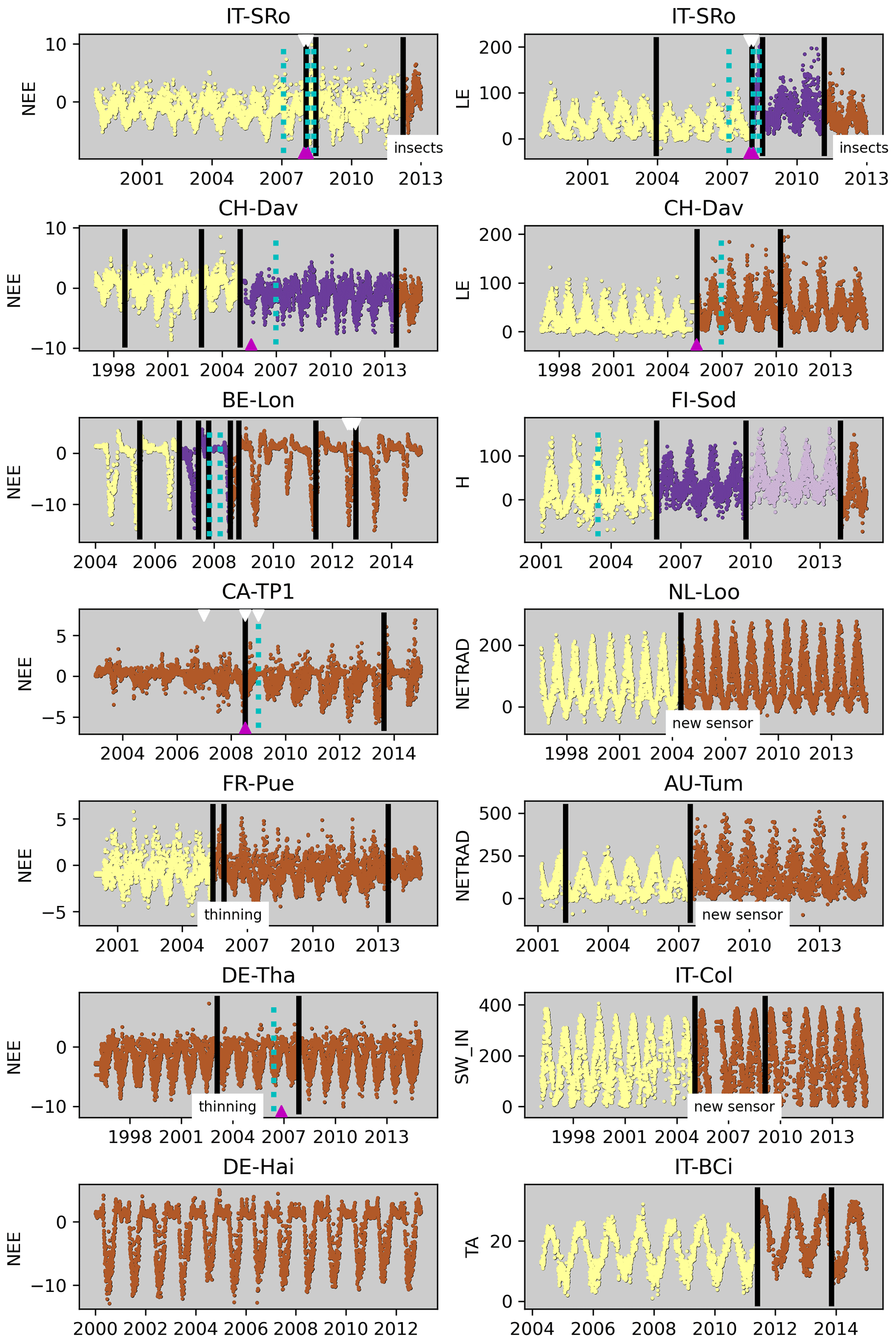
Figure 12Illustration of detected breaks for some sites and variables. Vertical black bars correspond to breaks exceeding nIQR = 1.5 (strict); an additional change in colour corresponds to bigger breaks (nIQR = 3, loose). Dates of changes in instrumentation recorded in BADMs are labelled as dotted cyan lines (sonic anemometer), magenta triangles (gas analyser), and a white triangle (measurement height). Other changes where only the year was given are shown as text.
Across FLUXNET 2015, large discontinuities (nIQR > 3) in LE are detected for about 25 % of sites; in NEE, SW_IN, and NETRAD for about 20 % of sites; and in H and TA for about 10 % of sites (Fig. 13). Considering very big discontinuities (up to nIQR = 6 and larger), we see that the fraction of affected sites levels off at about 15 % for LE, SW_IN, and NETRAD, suggesting that changes in the instrumentations of radiometers may be causing more frequent discontinuities in the data than perhaps anticipated. We find that, for the majority of long-term sites, at least one big discontinuity was detected for the radiation fluxes, LE, and NEE.
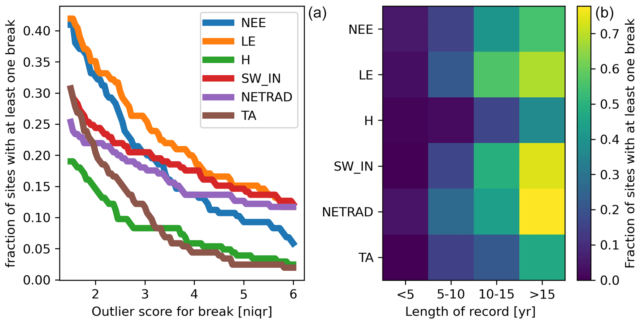
Figure 13Fraction of sites with at least one break detected for different variables as a function of the applied outlier score threshold (a) and as a function of record length (b) based on nIQR = 3.
4.1 Methodological considerations
The key objective of any data-screening approach is to distinguish between appropriate and inappropriate data, while there is some arbitrariness and context dependence in the definition of what is appropriate. We addressed this aspect from a conceptual point of view by flagging data that are inconsistent based on multiple expected relationships among variables, where the strictness of the inconsistency definition can be varied by the user according to specific demands and applications. The key question is on the effectiveness of the C2F algorithm in flagging, ideally, all inappropriate data while retaining, ideally, all appropriate data. The key challenges in assessing this are the lack of reference or validation data for inappropriate data and that inappropriate data are expected to be rare cases. In the following, we discuss methodological aspects related to erroneously flagging appropriate data (false positive) and erroneously not flagging inappropriate data (false negative).
4.1.1 Factors for potential false-positive and false-negative flagging
C2F is fundamentally based on the distribution of residuals from expected relationships among variables rather than on the distribution of the target variable itself. The latter is a common quality control procedure for identifying outliers, e.g. based on the boxplot rule, but flags extreme values in the tails of the distribution by construction and thus risks false-positive and systematic flagging. Our choice of working with residuals is preferable here because values in the tails of the target variable distribution are retained as long as deviations from expected relationships are not extreme. We showed that C2F is effective in retaining data under extreme temperature conditions (see Sect. 3.1).
Hence, it is relevant to assess whether detected inconsistencies, i.e. large deviations from expected relationships, can also be real rather than pointing to data issues. We addressed this aspect by distinguishing between hard and soft constraints (see Sect. 2.2.1), where, for soft constraints, large deviations do not force flagging of values immediately. Most soft constraints are related to ecosystem fluxes (Tables 2, S1) because, for example, functional changes in the ecosystem may change relationships between meteorological variables with the fluxes, as well as relationships between different fluxes. Flagging is only enforced when more than one soft constraint indicates an inconsistency. It is important to construct the different constraints to be independent from each other as much as possible. This approach of considering multiple indications of inconsistency essentially tries to minimize false positives and tries to avoid flagging data that appear to be unusual but might be real, while this obviously comes with the risk of having more false negatives.
The consideration of heteroscedasticity of residuals has been key in minimizing false positives and negatives. The fact that the variability in residuals typically increases with magnitude (Richardson et al., 2008) implies that we would get many false negatives at low magnitude and many false positives at high magnitude, leading to a severely biased and systematic pattern of flagging if not accounting for heteroscedasticity (Fig. 2). In the estimation procedure of the heteroscedasticity (Sect. S2), it was important to extrapolate the distribution properties of the residuals to the tails of the distribution of the target variable where they cannot be estimated empirically in order to minimize false positives there. This was not accounted for in previous methods based on binning residuals based on magnitude (Vitale et al., 2020). Some indications of elevated flagging frequencies under extreme temperature conditions (Fig. 11) may indicate some remaining uncertainties in accounting for heteroscedasticity, which is particularly challenging at the tails of distributions due to data scarcity.
The estimation of the outlier score is an adaptation of the boxplot rule, accounting for potential asymmetries in the distributions. This is preferable over excluding a fixed percentage of data, which is sometimes done. By varying the nIQR parameter, we can choose how strictly we apply C2F as this determines how far into the tails of the distribution of residuals a data point is allowed to fall. Increasing nIQR makes C2F become more loose, leading to fewer flagged data overall, as well as fewer false positives but more false negatives. Choosing the boxplot rule is common practice in identifying outliers as it is simple and avoids making assumptions about the underlying distribution. However, the expected probability of a data point in the tails of the distribution is certainly dependent on the specific properties of the distribution, in particular the skewness and kurtosis, which are very hard to estimate empirically in a robust way (Ritter, 2023). In addition, we did not account for sample size corrections of the boxplot rule (Ritter, 2023; Schwertman et al., 2004) in the current version since these are also sensitive to the assumptions of the underlying distribution. All these factors cause some uncertainty for false positives and false negatives.
Being able to define meaningful constraints is a prerequisite for C2F to work. For target variables where we have fewer constraints, like here, e.g. for TA and NEE, more false negatives must be expected. This means that C2F is less effective in detecting data issues for NEE and highlights the importance of dedicated checks and corrections being applied to the calculation of fluxes, especially under challenging conditions of rain, stable atmospheric stratification, sloping terrains, tall canopies, and appreciable storages. Practical issues due to the lack of data in evaluating a constraint obviously increase the risk of false negatives. Likewise, issues due to non-stationary behaviour of relationships due to, for example, changes in instrumentation increase the risk of false negatives because the overall distribution of residuals will be wider and thus more forgiving. Running C2F within segments identified by the detection of temporal discontinuities could improve this aspect in the future. Overall, we can expect that the more appropriate the flux tower data already are before we apply C2F, the better and more precise C2F will work in identifying remaining inconsistencies.
4.1.2 Detection and interpretation of discontinuities in the time series
Our detection of temporal discontinuities is based on model residuals rather than on the raw data of the flux tower variable. This is preferable because (1) the data typically show very large seasonal variations that would propagate to the test statistic, and (2) gap-filling of long gaps is not needed, which is particularly challenging in this context because it would require filling with realistic variability (including noise) to avoid artefacts in the distribution of the data.
We chose to use residuals from two models jointly in the estimation of the breaks: (1) a machine learning model based on environmental conditions and (2) a machine learning model based only on the day of the year and potential shortwave radiation that effectively performs a deseasonalization. The advantage of the first model is that it accounts for observed variations due to changes in environmental conditions. However, we found that the machine learning model was too flexible in some instances where the model predicted an obvious artefact in the distribution of a target variable because there was a concomitant change in one of the predictors. The latter can happen because the predictor variables are also flux tower data, e.g. if two instruments are modified at the same time or if the tower is moved or raised. This was the reason for additionally including the deviations from seasonality obtained from the second model. The residuals of both models were normalized to account for heteroscedasticity, which further minimizes differences in distributions due to different proportions of different seasons when calculating the test statistic.
Currently, discontinuities are flagged based on how unusual differences in distributions are using an outlier score calculated from a distribution of break severities pooled across all variables. While our definition for flagging temporal discontinuities is simple and allows for varying the threshold, it is clear that it is not directly related to whether a detected discontinuity is meaningful or relevant for a certain application. Further, pooling the distribution of break severity across all variables rather than evaluating per variable has the following advantages: (1) it allows for obtaining a larger sample size to better characterize the distribution, in particular its tail, and (2) it shows better comparability among variables in terms of which variables are more affected by breaks. At the same time, pooling across variables is not ideal from the perspective of hunting artefacts due to instrumentation changes since we expect more false positives for ecosystem fluxes compared to meteorological variables due to the possibility of real disruptions in the ecosystem.
The breakpoint detection is based on assessing changes in the distribution of residuals from machine learning models. This implies that any factors impacting the target variable distribution that were not accounted for in the modelling can elevate the test statistic. Beyond abrupt changes in instrumentation that we would like to flag ideally, other reasons for a change in the distribution of residuals can be natural or anthropogenic-disturbances-like events (e.g. insect outbreaks, fires, windthrows, harvest, thinning, crop rotation, other management practices) that change ecosystem properties. Also, gradual changes in the distribution of residuals could, in theory, cause the detection of a break, e.g. due to strong trends in (1) ecosystem properties, e.g. due to succession or post-disturbance recovery; (2) environmental conditions that are not modelled (e.g. CO2 fertilization); and (3) target variables due to drifting sensors.
From our results applied to FLUXNET 2015, we have some indications that the effect of trends does not cause a large proportion of flagging discontinuities. While we expect a trend in air temperatures in many long time series due to global warming, we find that the air temperature variable is among the variables that are least affected by detected discontinuities (see Sect. 3.2), probably because air temperature is comparatively easy to measure.
Overall, our results further suggest that detected discontinuities due to instrumentation artefacts seem to dominate over natural, real changes. We see, for example, relatively large differences in the frequencies of big discontinuities between radiation fluxes and temperature (Fig. 13) or between LE and H. Such large differences would not be expected if detected discontinuities were due to real environmental changes. Instead, these differences in the frequency of detected breaks among variables correspond to different levels of complexity for measuring variables: while temperature sensors are robust, long lasting, and require little maintenance, radiation sensors are sensitive to levelling, deterioration, or contamination and require more frequent maintenance and replacement. Sensible heat is measured by the sonic anemometer directly, which typically runs for years without major problems. For latent energy, the infrared gas analyser is needed additionally, and this requires more frequent calibrations, maintenance, and replacement.
Clearly, some of the detected discontinuities are due to real changes, as illustrated for some examples (Fig. 12). This implies that detected discontinuities require careful attention in order to judge whether they are due to an artefact or a real phenomenon, and it confirms the importance of complete metadata and ancillary data as a crucial set of information for the proper interpretation of the measurements.
4.2 Notes and recommendations for applications
4.2.1 Flagging inconsistent data
Adding or modifying constraints or the strictness parameter nIQR for custom applications is straightforward. Since almost all computational costs are associated with calculating intermediate diagnostics that are stored, it is straightforward and fast to obtain new flagging results for modified consistency strictness. This is particularly useful for assessing the relevance of the data quality–quantity trade-off for the conclusions of a specific application. If that is desired, we recommend recalculating the flags for nIQR, varying from 1.5 to 5, e.g. at intervals of 0.1, and finding the smallest nIQR at which flagging is indicated. This yields a more continuous representation of inconsistency and facilitates straightforward filtering. The recalculation of flags for different consistency strictness values is preferable over using the inconsistency score because the flagging takes additional considerations into account (see Sect. 2.2.4).
The approach for daily data outlined here can, in principle, be adapted to sub-daily data, but it would require modifying some of the constraints and settings. Hourly C2F could also help in detecting inconsistencies in radiation data for certain sun angles when parts of the tower infrastructure, like guy wires, may shade individual sensors. We developed the approach for daily data because these are still used most frequently in synthesis studies and because of the much smaller computational costs. For applications using sub-daily data, we recommend discarding all sub-daily data of a flagged daily value for now.
C2F delivers flags for individual daily data points for a variable and site, as well as flags for entire-site variables. While it is not feasible to scrutinize every flagged data point to make a decision on whether one wants to include this or not, we suggest that scrutinizing the entirety of the flagged site variables manually is feasible and recommended; i.e. the flagging of site variables is only meant to draw attention to potential data issues that require further investigation. This is particularly relevant because, for example, GPP from sites at the fringes of the tower distribution in climate space is more frequently flagged, and these sites are, in principle, particularly precious for global synthesis studies.
4.2.2 Flagging temporal discontinuities
The detected discontinuities in flux tower variables are meant to draw attention to potential artefacts in the data, which then require further investigation and judgement depending on the application and data needs. In particular, discontinuities in ecosystem fluxes can be due to real changes in the ecosystem, e.g. due to disturbances, harvest, crop rotations, or other management practices. While it is hard to formalize, we can provide some guidance on collecting indications of which of the reasons may apply based on logical reasoning. For a disturbance-like event in the ecosystem, we expect breaks in several ecosystem fluxes around the same time but not for meteorological variables like SW_IN and TA (or, at least, much less severe changes). In addition, we expect that a disturbance would shift the ecosystem NEE towards less carbon uptake on average. Detected discontinuities around the same time in ecosystem fluxes and meteorological variables may indicate a major change in the instrumentation infrastructure, such as raising or moving of the tower. To infer whether a flagged discontinuity is due to a trend in the variable, one could simply remove the trend in the residuals before inputting them to the calculation of the test statistic.
How to deal with detected discontinuities in the time series can also be very application dependent and may vary between discarding the site, keeping only the longest segment, running the analysis separately within segments, or not doing anything about it. Clearly, analysis targeting interannual variations or trends should consider discontinuities in the time series that could be artefacts of changes in the measurement setup.
4.3 Flagging patterns
Applying C2F to FLUXNET 2015 has revealed three major patterns of data inconsistencies: (1) comparatively large flagging frequencies for GPP and RECO, with a systematic pattern of more frequent flagging under dry–hot conditions, especially after rain; (2) comparatively frequent flagging for SW_IN and NETRAD; and (3) frequently detected discontinuities in long time series of LE, NEE, SW_IN, and NETRAD.
4.3.1 Flagged data points
The high proportions of flagged GPP and RECO data in dry seasons can be because the relationship between nighttime respiration and temperatures breaks down or because fast rain pulse responses get obscured by the moving-window approach used for NEE partitioning. For the daytime partitioning, we see a tendency toward more flagging at high temperatures and higher GPP compared to the nighttime method. Potentially, this is due to imperfect accounting of the VPD effect on GPP in the parameterized light response curves used to derive GPP_DT. While the absolute values of GPP and RECO are often quite small under such dry conditions, this issue causes comparatively little uncertainty for annual budgets. However, they imply some limits in our ability to better understand ecohydrological functioning under water stress and rain pulses. Respiration rain pulses were recently identified as a phenomenon of large-scale relevance for the carbon cycle (Metz et al., 2023; Rousk and Brangarí, 2022), and we recommend analysing those with flux tower data using NEE due to the issues of currently implemented methods for deriving RECO and GPP. Novel flux-partitioning methods like (Tramontana et al., 2020) that take water stress conditions into better account and avoid fitting in moving windows would be important complements to have in the near future.
Relatively frequent inconsistencies in radiation variables may be due to issues in correctly installing, calibrating, and maintaining the sensors. For example, quantum sensors for measuring photosynthetically active radiation are known to drift over time if not frequently calibrated. C2F could easily be extended to detect this specific drift problem by assessing trends in the residuals of the SW_IN vs. PPFD_IN constraint. Radiation data are crucial for the interpretation of ecosystem fluxes and are required as forcing variables for models. Clearly, faulty radiation inputs would cause faulty flux predictions. Furthermore, NETRAD is often used to estimate evaporative fraction as a water stress indicator and is needed for analysing or correcting the energy balance closure gap problem. This calls again to the importance of the maintenance of the sensors and the correct and full recording and reporting of all sensors replacements or calibrations in the metadata.
4.3.2 Flagged discontinuities in time series
We found that most long-term sites show discontinuities in terms of radiation variables, LE, and NEE. Obviously, this might have large implications for studying many outstanding questions regarding interannual variations and trends of ecosystem fluxes using FLUXNET. While such discontinuities can also be due to real changes in the ecosystem, we have indications that data issues are likely the prevalent reason (see Sect. 3.2). Even if half of those would be attributable to false alarms in a very conservative scenario, this would still represent a very relevant problem for the community.
Comparatively rarely detected discontinuities in TA and H could be because the associated instruments are quite robust and long lasting. In contrast, radiation sensors need replacement and maintenance more frequently and are subject to drifts, which could explain more frequently detected discontinuities in radiation variables. For LE and NEE in particular, the involvement of two different sensors in the measurements – and, for closed-path systems, an additional tube that also requires substitutions or maintenance – could increase the chances of temporal discontinuities. In addition, changes in the flux calculations, corrections, and filtering can be reasons for temporal discontinuities. It would be important to better understand what aspects related to instrumentation and maintenance change are causing the main problems here to facilitate consistent long time series in the future. Also, in this case, the availability of metadata about sensors, setup changes, or major disturbances or management activities at the sites are very important for the interpretation of detected discontinuities and could allow for more tailored approaches in the future. In the case of meteorological variables, redundant measurements could be used to support the construction of a consistent time series in the case of sensor replacement. This would improve C2F overall as more constraints could be defined and used.
Using expert knowledge and experience, we designed and implemented C2F, a complementary data-screening algorithm for flux tower data based on the principle of detecting inconsistencies. It is fully automated, transparent, follows objective principles, and delivers simple Boolean flags that are straightforward to use.
Clearly, C2F is not perfect – it complements and cannot replace the typical quality control of flux tower data done by PIs and during centralized processing like ICOS or NEON. In fact, it relies on the assumption that the vast majority of data are appropriate already. The quality of our flags also relies on data availability in terms of variables, i.e. the number of constraints that can be used, and data quantity for robust estimation of the statistical metrics used. To further develop and improve C2F, it would be desirable to be able to benchmark it objectively using a large set of synthetic data, where flux tower data, with all their potential issues and noise properties, are realistically emulated with labels for inappropriate data that are available.
Applying C2F to the FLUXNET2015 dataset uncovered, for instance, issues in the NEE flux partitioning into GPP and RECO under dry and hot conditions, as well as temporal discontinuities in long time series of, for example, LE and NEE. While the potential existence of such problems is no surprise for eddy covariance specialists, C2F provides associated flags, which were not available before. This is especially useful for synthesis activities, ecosystem modellers, or remote sensing integration with machine learning. We therefore hope that C2F helps in making scientific progress, in improving FLUXCOM and process-based models, and in flux tower data becoming more accessible and used across communities. In addition, C2F could help in assisting PIs to assess data consistency before submission to regional networks, and it could help in accelerating feedback loops between PIs and centralized processing units of regional networks if it were to be implemented in ONEFLUX and run routinely by the regional networks.
The code with a user interface is available on Zenodo (https://doi.org/10.5281/zenodo.10593332, Nelson et al., 2024a).
The flagging results for FLUXNET 2015 are available on Zenodo (https://doi.org/10.5281/zenodo.10567776, Nelson et al., 2024b).
The supplement related to this article is available online at: https://doi.org/10.5194/bg-21-1827-2024-supplement.
MJ developed and implemented the methodology, performed the analysis, and drafted most of the paper. JN helped with coding and applied the code to FLUXNET data. JN and TW developed code for a user interface. MM, TEM, DP, TW, and MR contributed expert knowledge on eddy covariance quality controlling. All the authors provided intellectual input to the work and paper.
The contact author has declared that none of the authors has any competing interests.
Publisher’s note: Copernicus Publications remains neutral with regard to jurisdictional claims made in the text, published maps, institutional affiliations, or any other geographical representation in this paper. While Copernicus Publications makes every effort to include appropriate place names, the final responsibility lies with the authors.
The authors acknowledge the reviewers who helped to improve the clarity of the paper. Sophia Walther acknowledges support from the European Space Agency for the Living Planet Fellowship Vad3emecum.
This research has been supported by Horizon 2020 (grant nos. 958927 and 820852), the EU – Next Generation EU (grant no. IR0000032), and the European Space Agency (ESA) (grant no. 4000134598/21/I-NB).
The article processing charges for this open-access publication were covered by the Max Planck Society.
This paper was edited by Akihiko Ito and reviewed by Dennis Baldocchi and one anonymous referee.
Baldocchi, D. D.: How eddy covariance flux measurements have contributed to our understanding of Global Change Biology, Glob. Change Biol., 26, 242–260, https://doi.org/10.1111/gcb.14807, 2020.
Bodesheim, P., Jung, M., Gans, F., Mahecha, M. D., and Reichstein, M.: Upscaled diurnal cycles of land–atmosphere fluxes: a new global half-hourly data product, Earth Syst. Sci. Data, 10, 1327–1365, https://doi.org/10.5194/essd-10-1327-2018, 2018.
Breiman, L.: Random forests, Mach. Learn., 45, 5–32, https://doi.org/10.1023/a:1010933404324, 2001.
Falge, E., Aubinet, M., Bakwin, P., Baldocchi, D., Berbigier, P., Bernhofer, C., Black, T. A., Ceulemans, R., Davis, K., Dolman, A. J., Goldstein, A., Goulden, M. L., Granier, A., Hollinger, D., Jarvis, P. G., Jensen, N., Pilegaard, K., Katul, G., Kyaw Tha Paw, P., Law, B. E., Lindroth, A., Loustau, D., Mahli, Y., Monson, R., Moncrieff, P., Moors, E., Munger, J. W., Meyers, T., Oechel, W., Schulze, E. D., Thorgeirsson, H., Tenhunen, J., Valentini, R., Verma, S. B., Vesala, T., and Wofsy, S. C.: FLUXNET Marconi Conference Gap-Filled Flux and Meteorology Data, 1992–2000, ORNL DAAC, Oak Ridge, Tennessee, USA, https://doi.org/10.3334/ORNLDAAC/811, 2005.
Fischler, M. A. and Bolles, R. C.: Random sample consensus: a paradigm for model fitting with applications to image analysis and automated cartography, Commun. ACM, 24, 381–395, https://doi.org/10.1145/358669.358692, 1981.
Franz, D., Acosta, M., Altimir, N., Arriga, N., Arrouays, D., Aubinet, M., Aurela, M., Ayres, E., López-Ballesteros, A., Barbaste, M., Berveiller, D., Biraud, S., Boukir, H., Brown, T., Brümmer, C., Buchmann, N., Burba, G., Carrara, A., Cescatti, A., Ceschia, E., Clement, R., Cremonese, E., Crill, P., Darenova, E., Dengel, S., D'Odorico, P., Gianluca, F., Fleck, S., Fratini, G., Fuß, R., Gielen, B., Gogo, S., Grace, J., Graf, A., Grelle, A., Gross, P., Grünwald, T., Haapanala, S., Hehn, M., Heinesch, B., Heiskanen, J., Herbst, M., Herschlein, C., Hörtnagl, L., Hufkens, K., Ibrom, A., Jolivet, C., Joly, L., Jones, M., Kiese, R., Klemedtsson, L., Kljun, N., Klumpp, K., Kolari, P., Kolle, O., Kowalski, A., Kutsch, W., Laurila, T., De Ligne, A., Linder, S., Lindroth, A., Lohila, A., Longdoz, B., Mammarella, I., Manise, T., Marañon-Jimenez, S., Matteucci, G., Mauder, M., Meier, P., Merbold, L., Mereu, S., Metzger, S., Migliavacca, M., Mölder, M., Montagnani, L., Moureaux, C., Nelson, D., Nemitz, E., Nicolini, G., Nilsson, M. B., Op de Beeck, M., Osborne, B., Ottosson Löfvenius, M., Pavelka, M., Peichl, M., Peltola, O., Pihlatie, M., Pitacco, A., Pokorny, R., Pumpanen, J., Ratié, C., Schrumpf, M., Sedlák, P., Serrano Ortiz, P., Siebicke, L., Šigut, L., Silvennoinen, H., Simioni, G., Skiba, U., Sonnentag, O., Soudani, K., Soulé, P., Steinbrecher, R., Tallec, T., Thimonier, A., Tuittila, E.-S., Tuovinen, J.-P., Vestin, P., Vincent, G., Vincke, C., Vitale, D., Waldner, P., Weslien, P., Wingate, L., Wohlfahrt, G., Zahniser, M., and Vesala, T.: Towards long-term standardised carbon and greenhouse gas observations for monitoring Europe's terrestrial ecosystems: a review, Int. Agrophys., 32, 439–455, https://doi.org/10.1515/intag-2017-0039, 2018.
Heiskanen, J., Brümmer, C., Buchmann, N., Calfapietra, C., Chen, H., Gielen, B., Gkritzalis, T., Hammer, S., Hartman, S., Herbst, M., Janssens, I. A., Jordan, A., Juurola, E., Karstens, U., Kasurinen, V., Kruijt, B., Lankreijer, H., Levin, I., Linderson, M.-L., Loustau, D., Merbold, L., Myhre, C. L., Papale, D., Pavelka, M., Pilegaard, K., Ramonet, M., Rebmann, C., Rinne, J., Rivier, L., Saltikoff, E., Sanders, R., Steinbacher, M., Steinhoff, T., Watson, A., Vermeulen, A. T., Vesala, T., Vítková, G., and Kutsch, W.: The Integrated Carbon Observation System in Europe, B. Am. Meteorol. Soc., 103, E855–E872, https://doi.org/10.1175/bams-d-19-0364.1, 2022.
Jung, M., Koirala, S., Weber, U., Ichii, K., Gans, F., Camps-Valls, G., Papale, D., Schwalm, C., Tramontana, G., and Reichstein, M.: The FLUXCOM ensemble of global land-atmosphere energy fluxes, Sci. Data, 6, 74, https://doi.org/10.1038/s41597-019-0076-8, 2019.
Jung, M., Schwalm, C., Migliavacca, M., Walther, S., Camps-Valls, G., Koirala, S., Anthoni, P., Besnard, S., Bodesheim, P., Carvalhais, N., Chevallier, F., Gans, F., Goll, D. S., Haverd, V., Köhler, P., Ichii, K., Jain, A. K., Liu, J., Lombardozzi, D., Nabel, J. E. M. S., Nelson, J. A., O'Sullivan, M., Pallandt, M., Papale, D., Peters, W., Pongratz, J., Rödenbeck, C., Sitch, S., Tramontana, G., Walker, A., Weber, U., and Reichstein, M.: Scaling carbon fluxes from eddy covariance sites to globe: synthesis and evaluation of the FLUXCOM approach, Biogeosciences, 17, 1343–1365, https://doi.org/10.5194/bg-17-1343-2020, 2020.
Lasslop, G., Reichstein, M., Papale, D., Richardson, A. D., Arneth, A., Barr, A., Stoy, P., and Wohlfahrt, G.: Separation of net ecosystem exchange into assimilation and respiration using a light response curve approach: critical issues and global evaluation, Glob. Change Biol., 16, 187–208, 2010.
Metz, E.-M., Vardag, S. N., Basu, S., Jung, M., Ahrens, B., El-Madany, T., Sitch, S., Arora, V. K., Briggs, P. R., Friedlingstein, P., Goll, D. S., Jain, A. K., Kato, E., Lombardozzi, D., Nabel, J. E. M. S., Poulter, B., Séférian, R., Tian, H., Wiltshire, A., Yuan, W., Yue, X., Zaehle, S., Deutscher, N. M., Griffith, D. W. T., and Butz, A.: Soil respiration–driven CO2 pulses dominate Australia's flux variability, Science, 379, 1332–1335, https://doi.org/10.1126/science.add7833, 2023.
Metzger, S., Durden, D., Florian, C., Luo, H., Pingintha-Durden, N., and Xu, K.: Algorithm theoretical basis document: eddy-covariance data products bundle, National Ecological Observatory Network, NEON.DOC.004571, Revision A (2018-04-30), http://data.neonscience.org/documents (last access: 9 April 2024), Boulder, USA, 55 pp., 2018.
Nelson, J., Wutzler, T., and Jung, M.: c2f_fluxnet (v1.0), Zenodo [code], https://doi.org/10.5281/zenodo.10593332, 2024a.
Nelson, J., Wutzler, T., Jung, M., and FLUXCOM-X Team: C2F Flags (1.0), Zenodo [data set], https://doi.org/10.5281/zenodo.10567776, 2024b.
Papale, D., Reichstein, M., Aubinet, M., Canfora, E., Bernhofer, C., Kutsch, W., Longdoz, B., Rambal, S., Valentini, R., Vesala, T., and Yakir, D.: Towards a standardized processing of Net Ecosystem Exchange measured with eddy covariance technique: algorithms and uncertainty estimation, Biogeosciences, 3, 571–583, https://doi.org/10.5194/bg-3-571-2006, 2006.
Pastorello, G., Agarwal, D., Papale, D., Samak, T., Trotta, C., Ribeca, A., Poindexter, C., Faybishenko, B., Gunter, D., Hollowgrass, R., and Canfora, E.: Observational Data Patterns for Time Series Data Quality Assessment, 2014 IEEE 10th International Conference on e-Science, 20–24 October 2014, 271–278, https://doi.org/10.1109/eScience.2014.45, 2014.
Pastorello, G., Trotta, C., Canfora, E., Chu, H., Christianson, D., Cheah, Y.-W., Poindexter, C., Chen, J., Elbashandy, A., Humphrey, M., Isaac, P., Polidori, D., Reichstein, M., Ribeca, A., van Ingen, C., Vuichard, N., Zhang, L., Amiro, B., Ammann, C., Arain, M. A., Ardö, J., Arkebauer, T., Arndt, S. K., Arriga, N., Aubinet, M., Aurela, M., Baldocchi, D., Barr, A., Beamesderfer, E., Marchesini, L. B., Bergeron, O., Beringer, J., Bernhofer, C., Berveiller, D., Billesbach, D., Black, T. A., Blanken, P. D., Bohrer, G., Boike, J., Bolstad, P. V., Bonal, D., Bonnefond, J.-M., Bowling, D. R., Bracho, R., Brodeur, J., Brümmer, C., Buchmann, N., Burban, B., Burns, S. P., Buysse, P., Cale, P., Cavagna, M., Cellier, P., Chen, S., Chini, I., Christensen, T. R., Cleverly, J., Collalti, A., Consalvo, C., Cook, B. D., Cook, D., Coursolle, C., Cremonese, E., Curtis, P. S., D'Andrea, E., da Rocha, H., Dai, X., Davis, K. J., Cinti, B. D., Grandcourt, A. d., Ligne, A. D., De Oliveira, R. C., Delpierre, N., Desai, A. R., Di Bella, C. M., Tommasi, P. d., Dolman, H., Domingo, F., Dong, G., Dore, S., Duce, P., Dufrêne, E., Dunn, A., Dušek, J., Eamus, D., Eichelmann, U., ElKhidir, H. A. M., Eugster, W., Ewenz, C. M., Ewers, B., Famulari, D., Fares, S., Feigenwinter, I., Feitz, A., Fensholt, R., Filippa, G., Fischer, M., Frank, J., Galvagno, M., Gharun, M., Gianelle, D., Gielen, B., Gioli, B., Gitelson, A., Goded, I., Goeckede, M., Goldstein, A. H., Gough, C. M., Goulden, M. L., Graf, A., Griebel, A., Gruening, C., Grünwald, T., Hammerle, A., Han, S., Han, X., Hansen, B. U., Hanson, C., Hatakka, J., He, Y., Hehn, M., Heinesch, B., Hinko-Najera, N., Hörtnagl, L., Hutley, L., Ibrom, A., Ikawa, H., Jackowicz-Korczynski, M., Janouš, D., Jans, W., Jassal, R., Jiang, S., Kato, T., Khomik, M., Klatt, J., Knohl, A., Knox, S., Kobayashi, H., Koerber, G., Kolle, O., Kosugi, Y., Kotani, A., Kowalski, A., Kruijt, B., Kurbatova, J., Kutsch, W. L., Kwon, H., Launiainen, S., Laurila, T., Law, B., Leuning, R., Li, Y., Liddell, M., Limousin, J.-M., Lion, M., Liska, A. J., Lohila, A., López-Ballesteros, A., López-Blanco, E., Loubet, B., Loustau, D., Lucas-Moffat, A., Lüers, J., Ma, S., Macfarlane, C., Magliulo, V., Maier, R., Mammarella, I., Manca, G., Marcolla, B., Margolis, H. A., Marras, S., Massman, W., Mastepanov, M., Matamala, R., Matthes, J. H., Mazzenga, F., McCaughey, H., McHugh, I., McMillan, A. M. S., Merbold, L., Meyer, W., Meyers, T., Miller, S. D., Minerbi, S., Moderow, U., Monson, R. K., Montagnani, L., Moore, C. E., Moors, E., Moreaux, V., Moureaux, C., Munger, J. W., Nakai, T., Neirynck, J., Nesic, Z., Nicolini, G., Noormets, A., Northwood, M., Nosetto, M., Nouvellon, Y., Novick, K., Oechel, W., Olesen, J. E., Ourcival, J.-M., Papuga, S. A., Parmentier, F.-J., Paul-Limoges, E., Pavelka, M., Peichl, M., Pendall, E., Phillips, R. P., Pilegaard, K., Pirk, N., Posse, G., Powell, T., Prasse, H., Prober, S. M., Rambal, S., Rannik, Ü., Raz-Yaseef, N., Rebmann, C., Reed, D., Dios, V. R. d., Restrepo-Coupe, N., Reverter, B. R., Roland, M., Sabbatini, S., Sachs, T., Saleska, S. R., Sánchez-Cañete, E. P., Sanchez-Mejia, Z. M., Schmid, H. P., Schmidt, M., Schneider, K., Schrader, F., Schroder, I., Scott, R. L., Sedlák, P., Serrano-Ortíz, P., Shao, C., Shi, P., Shironya, I., Siebicke, L., Šigut, L., Silberstein, R., Sirca, C., Spano, D., Steinbrecher, R., Stevens, R. M., Sturtevant, C., Suyker, A., Tagesson, T., Takanashi, S., Tang, Y., Tapper, N., Thom, J., Tomassucci, M., Tuovinen, J.-P., Urbanski, S., Valentini, R., van der Molen, M., van Gorsel, E., van Huissteden, K., Varlagin, A., Verfaillie, J., Vesala, T., Vincke, C., Vitale, D., Vygodskaya, N., Walker, J. P., Walter-Shea, E., Wang, H., Weber, R., Westermann, S., Wille, C., Wofsy, S., Wohlfahrt, G., Wolf, S., Woodgate, W., Li, Y., Zampedri, R., Zhang, J., Zhou, G., Zona, D., Agarwal, D., Biraud, S., Torn, M., and Papale, D.: The FLUXNET2015 dataset and the ONEFlux processing pipeline for eddy covariance data, Sci. Data, 7, 225, https://doi.org/10.1038/s41597-020-0534-3, 2020.
Rebmann, C., Aubinet, M., Schmid, H., Arriga, N., Aurela, M., Burba, G., Clement, R., De Ligne, A., Fratini, G., Gielen, B., Grace, J., Graf, A., Gross, P., Haapanala, S., Herbst, M., Hörtnagl, L., Ibrom, A., Joly, L., Kljun, N., Kolle, O., Kowalski, A., Lindroth, A., Loustau, D., Mammarella, I., Mauder, M., Merbold, L., Metzger, S., Mölder, M., Montagnani, L., Papale, D., Pavelka, M., Peichl, M., Roland, M., Serrano-Ortiz, P., Siebicke, L., Steinbrecher, R., Tuovinen, J.-P., Vesala, T., Wohlfahrt, G., and Franz, D.: ICOS eddy covariance flux-station site setup: a review, Int. Agrophys., 32, 471–494, https://doi.org/10.1515/intag-2017-0044, 2018.
Reichstein, M., Falge, E., Baldocchi, D., Papale, D., Valentini, R., Aubinet, M., Berbigier, P., Bernhofer, C., Buchmann, N., Gilmanov, T., Granier, A., Grünwald, T., Havránková, K., Janous, D., Knohl, A., Laurela, T., Lohila, A., Loustau, D., Matteucci, G., Meyers, T., Miglietta, F., Ourcival, J.-M., Rambal, S., Rotenberg, E., Sanz, M., Seufert, G., Vaccari, F., Vesala, T., and Yakir, D.: On the separation of net ecosystem exchange into assimilation and ecosystem respiration: review and improved algorithm, Glob. Change Biol., 11, 1424–1439, 2005.
Richardson, A. D., Mahecha, M. D., Falge, E., Kattge, J., Moffat, A. M., Papale, D., Reichstein, M., Stauch, V. J., Braswell, B. H., Churkina, G., Kruijt, B., and Hollinger, D. Y.: Statistical properties of random CO2 flux measurement uncertainty inferred from model residuals, Agr. Forest Meteorol., 148, 38–50, 2008.
Ritter, F.: Technical note: A procedure to clean, decompose, and aggregate time series, Hydrol. Earth Syst. Sci., 27, 349–361, https://doi.org/10.5194/hess-27-349-2023, 2023.
Rousk, J. and Brangarí, A. C.: Do the respiration pulses induced by drying–rewetting matter for the soil–atmosphere carbon balance?, Glob. Change Biol., 28, 3486–3488, https://doi.org/10.1111/gcb.16163, 2022.
Sabbatini, S., Mammarella, I., Arriga, N., Fratini, G., Graf, A., Hörtnagl, L., Ibrom, A., Longdoz, B., Mauder, M., Merbold, L., Metzger, S., Montagnani, L., Pitacco, A., Rebmann, C., Sedlák, P., Šigut, L., Vitale, D., and Papale, D.: Eddy covariance raw data processing for CO2 and energy fluxes calculation at ICOS ecosystem stations, Int. Agrophys., 32, 495–515, https://doi.org/10.1515/intag-2017-0043, 2018.
Schimel, D., Hargrove, W., Hoffman, F., and MacMahon, J.: NEON: a hierarchically designed national ecological network, Front. Ecol. Environ., 5, 59–59, https://doi.org/10.1890/1540-9295(2007)5[59:NAHDNE]2.0.CO;2, 2007.
Schwertman, N. C., Owens, M. A., and Adnan, R.: A simple more general boxplot method for identifying outliers, Comput. Stat. Data An., 47, 165–174, https://doi.org/10.1016/j.csda.2003.10.012, 2004.
Stekhoven, D. J. and Bühlmann, P.: MissForest – non-parametric missing value imputation for mixed-type data, Bioinformatics, 28, 112–118, https://doi.org/10.1093/bioinformatics/btr597, 2011.
Szekely, G. and Rizzo, M.: Testing for equal distributions in high dimension, InterStat, 5, 1–15, 2004.
Tramontana, G., Jung, M., Schwalm, C. R., Ichii, K., Camps-Valls, G., Ráduly, B., Reichstein, M., Arain, M. A., Cescatti, A., Kiely, G., Merbold, L., Serrano-Ortiz, P., Sickert, S., Wolf, S., and Papale, D.: Predicting carbon dioxide and energy fluxes across global FLUXNET sites with regression algorithms, Biogeosciences, 13, 4291–4313, https://doi.org/10.5194/bg-13-4291-2016, 2016.
Tramontana, G., Migliavacca, M., Jung, M., Reichstein, M., Keenan, T. F., Camps-Valls, G., Ogee, J., Verrelst, J., and Papale, D.: Partitioning net carbon dioxide fluxes into photosynthesis and respiration using neural networks, Glob. Change Biol., 26, 5235–5253, https://doi.org/10.1111/gcb.15203, 2020.
Vitale, D., Fratini, G., Bilancia, M., Nicolini, G., Sabbatini, S., and Papale, D.: A robust data cleaning procedure for eddy covariance flux measurements, Biogeosciences, 17, 1367–1391, https://doi.org/10.5194/bg-17-1367-2020, 2020.