Timescale dependence of airborne fraction and underlying climate–carbon-cycle feedbacks for weak perturbations in CMIP5 models

The response of the global climate–carbon-cycle system to anthropogenic perturbations happens differently at different timescales. The unravelling of the memory structure underlying this timescale dependence is a major challenge in climate research. Recently the widely applied α–β–γ framework proposed by Friedlingstein et al. (2003) to quantify climate–carbon-cycle feedbacks has been generalized to account also for such internal memory. By means of this generalized framework, we investigate the timescale dependence of the airborne fraction for a set of Earth system models that participated in CMIP5 (Coupled Model Intercomparison Project Phase 5). The analysis is based on published simulation data from C⁴MIP-type (Coupled Climate–Carbon Cycle Model Intercomparison) experiments with these models. Independently of the considered scenario, the proposed generalization describes at global scale the reaction of the climate–carbon system to sufficiently weak perturbations. One prediction from this theory is how the timescale-resolved airborne fraction depends on the underlying feedbacks between climate and the carbon cycle. These feedbacks are expressed as timescale-resolved functions depending solely on analogues of the α, β, and γ sensitivities, introduced in the generalized framework as linear response functions. In this way a feedback-dependent quantity (airborne fraction) is predicted from feedback-independent quantities (the sensitivities). This is the key relation underlying our study. As a preparatory step, we demonstrate the predictive power of the generalized framework exemplarily for simulations with the Max Planck Institute (MPI) Earth System Model. The whole approach turns out to be valid for perturbations of up to an about 100 ppm CO₂ rise above the pre-industrial level; beyond this value the response becomes non-linear. By means of the generalized framework we then derive the timescale dependence of the airborne fraction from the underlying climate–carbon-cycle feedbacks for an ensemble of CMIP5 models. Our analysis reveals that for all studied CMIP5 models (1) the total climate–carbon-cycle feedback is negative at all investigated timescales, (2) the airborne fraction generally decreases for increasing timescales, and (3) the land biogeochemical feedback dominates the model spread in the airborne fraction at all these timescales. Qualitatively similar results were previously found by employing the original α–β–γ framework to particular perturbation scenarios, but our study demonstrates that, although obtained from particular scenario simulations, they are characteristics of the coupled climate–carbon-cycle system as such, valid at all considered timescales. These more general conclusions are obtained by accounting for the internal memory of the system as encoded in the generalized sensitivities, which in contrast to the original α, β, and γ are scenario-independent.

1 Introduction

The global carbon cycle plays a key role in determining the sensitivity of Earth's climate to anthropogenic emissions from fossil-fuel burning, cement production, and land-use change. The increase in atmospheric CO₂ concentrations driven by those emissions is considered the main radiative forcing driving climate change (see e.g. Gulev et al., 2021, Fig. 2.10). But to infer the resulting changes in atmospheric CO₂ it is not sufficient to consider anthropogenic emissions alone; also the response of the global carbon cycle to these emissions must be taken into account. In reaction to rising emissions, land and ocean store increasing amounts of carbon, on average 56 % of emissions, a number that stayed surprisingly constant over the last 6 decades (Canadell et al., 2021, Fig. 5.7). This storage fraction strongly depends on environmental conditions: in years with a positive phase of the El Niño–Southern Oscillation (ENSO) it can be as low as 20 %, while in negative phases it may rise up to 75 % (Canadell et al., 2021, Fig. 5.7). One must thus suspect that with rising atmospheric CO₂ the resulting climate change will affect this fraction of emissions stored away with potentially large consequences for the amount of anthropogenic CO₂ remaining in the atmosphere. In this way, the carbon cycle may either slow or accelerate climatic changes resulting from anthropogenic emissions. Understanding the dynamics of this cycle, and in particular how it responds to perturbations from emissions and interferes with climate, thus constitutes an essential step in advancing climate research (Marotzke et al., 2017).

To gain insight into this combined dynamics of carbon cycle and climate, one must in particular study climate–carbon-cycle feedbacks. Such feedbacks arise from the already mentioned reaction of the global carbon cycle to a change in atmospheric CO₂ that may amplify or counteract the initial change. For example, a rise in CO₂ concentrations caused by fossil-fuel emissions drives CO₂ into the ocean by increasing the difference between the CO₂ partial pressure in the atmosphere and that in surface waters (Takahashi et al., 2009). This flux of CO₂ into the ocean reduces the initial increase in atmospheric CO₂. On the other hand, increasing atmospheric CO₂ leads by the greenhouse effect to a rise in air temperatures. The warmer climate, in turn, leads to an acceleration of soil microbial activity and thereby to an increase in soil respiration rates (Raich and Potter, 1995). The resulting enhanced land CO₂ flux into the atmosphere leads to even more CO₂ in the atmosphere so that the initial increase in atmospheric CO₂ is amplified. In principle, the global response of the whole carbon cycle to emissions may be quantified by summing the contributions from all such feedback mechanisms.

Depending on the speed at which the various feedbacks unfold, climate change may develop differently. Generally, the dynamics of the coupled climate–carbon-cycle system arising in response to perturbations depends on the spectrum of internal timescales of the various processes involved in the response. For instance, the speed at which global climate is warming in reaction to anthropogenic emissions depends largely on the rate at which the oceans can take up heat, and this rate – actually an inverse timescale – is determined by the temporal characteristics of the internal ocean dynamics, like the rate of mixing between upper and deep ocean and the speed at which heat is re-distributed by ocean currents. Similar remarks apply to the uptake and re-distribution of CO₂ by the oceans. An indication of the involved timescales is obtained by noting that most of the carbon taken up by the ocean since pre-industrial times still resides in its upper layers (74 % in the top 700 m; Frölicher et al., 2015). For land, the temporal characteristics of the response of the carbon cycle to rising CO₂ is determined by the turnover times of the various biogeochemical processes by which CO₂ is sequestered and once more decomposed in the various ecosystems. It is well known that in particular our incomplete knowledge of the internal timescales of the land carbon cycle is severely limiting our ability to predict the development of the land carbon sink (Todd-Brown et al., 2013; Friend et al., 2014; Exbrayat et al., 2014; Koven et al., 2015; He et al., 2016; Yan et al., 2017; Zhou et al., 2018). To improve the understanding of the dynamics of coupled climate–carbon-cycle system one thus needs to investigate together with the feedbacks also the issue of internal timescales.

Concerning the analysis of feedbacks, a large step forward was the seminal work by Friedlingstein et al. (2003), who proposed a mathematical framework to quantify their contributions to the response. The basic idea underlying their α–β–γ framework is that at global scale one can identify two types of climate–carbon-cycle feedback: a “biogeochemical feedback”, which arises through the direct effect of changes in atmospheric CO₂ concentrations on global carbon stocks, and a “radiative feedback”, which affects the carbon cycle indirectly from the change in climate that arises from the radiative forcing of CO₂ perturbations. Key elements of this framework to quantify the two types of feedback – also known as carbon-concentration and carbon–climate feedback (Arora et al., 2013) – are the β and γ sensitivities that, respectively, characterize the response of stored land and/or ocean carbon to changes in CO₂ and in climate. As in studies of the physical system by means of “pattern scaling” (e.g. Mitchell, 2003), climate is in this framework collectively represented by the single quantity temperature – whose sensitivity to CO₂ perturbations is quantified by α. The framework of Friedlingstein et al. (2003) led to important insights into the role of climate–carbon-cycle feedbacks for climate change and stimulated a vast amount of research in the field (Friedlingstein et al., 2006; Gregory et al., 2009; Arneth et al., 2010; Zickfeld et al., 2011; Boer and Arora, 2013; Arora et al., 2013; Schwinger et al., 2014; Friedlingstein et al., 2014; Friedlingstein, 2015; Adloff et al., 2018; Williams et al., 2019; Goodwin et al., 2019; Jones and Friedlingstein, 2020).

Quantitative results on the size of global climate–carbon-cycle feedbacks were particularly obtained as part of the Coupled Climate–Carbon Cycle Model Intercomparison (C⁴MIP) project (Friedlingstein et al., 2013–2016; Arora et al., 2020) from Earth system simulations tailored for the application of the α–β–γ framework. In terms of radiative forcing, when raising atmospheric CO₂ at a fixed rate of 1 % per year from its pre-industrial value to 4 times this value, the negative biogeochemical feedback is more than 4 times stronger than the positive radiative feedback (Canadell et al., 2021). This results in a net land and ocean carbon sequestration over the whole simulation period of between 33 % and 50 % across the participating models (Arora et al., 2020). Most of the spread in these numbers arises from differences in the representation of land carbon cycling in the various models, in particular from the internal timescales assumed for the turnover of vegetation and soils (Arora et al., 2020).

The size of these feedbacks depends on the considered timescale (e.g. Enting, 2022). In the original α–β–γ framework, this timescale dependence shows up only implicitly (see discussion in Sect. 2), so results from this framework are specific to the considered perturbation scenario (Gregory et al., 2009; Torres Mendonça et al., 2021b). This limitation is overcome by the recently proposed generalization of the α–β–γ framework (Heimann, 2014; Rubino et al., 2016; Enting and Clisby, 2019; Enting, 2022) that instead explicitly quantifies the timescale dependence of the climate–carbon-cycle feedbacks independently of the scenario. Here generalized sensitivities α, β, and γ are introduced as time-dependent linear response functions, where the term “linear” indicates that they specify the response only to linear order in a Volterra expansion of the response into the perturbation (see Torres Mendonça et al., 2021b); practically this means that this approach applies only as long as the perturbations are sufficiently weak. As will be discussed below, in principle this generalization gives – at a globally aggregated level – a complete description of the linear dynamics of the coupled climate and carbon cycle in terms of the responses and feedbacks at different timescales.

In the present study we employ this generalized framework to study the role of feedbacks and their timescale dependence for airborne fraction. Airborne fraction is classically defined as the fraction of emitted CO₂ that stays in the atmosphere after accounting for the induced land and ocean uptake. Accordingly, airborne fraction quantifies the amount of emissions that effectively contributes to climatic change and is therefore a key quantity of climate research (Oeschger and Heimann, 1983). It is closely related to the climate–carbon-cycle feedbacks because, as discussed above, the reduction in atmospheric CO₂ caused by ocean and land uptake depends itself on the changes in atmospheric CO₂ induced by the emissions. Because of its importance, much effort has been put into quantifying and investigating the airborne fraction (e.g. Canadell et al., 2007; Raupach et al., 2008; Archer et al., 2009; Gregory et al., 2009; Gloor et al., 2010; Jones et al., 2013; Le Quéré et al., 2009; Raupach et al., 2014; Bennedsen et al., 2019). The remarkable constancy of the airborne fraction over the last decades – a consequence of the above-mentioned constancy of the land and ocean carbon storage fraction – indicates that land and ocean uptake has not saturated yet, so their response is still linear. But as with the original α, β, and γ sensitivities, this classical definition of airborne fraction also neglects that its value must depend on the internal timescales at which the land and ocean carbon cycles react to emissions (see e.g. Enting, 2007). Addressing this timescale dependence, Raupach (2013) argues that the observed constancy of the airborne fraction is actually only a reflection of the linearity of the response of land and ocean carbon reservoirs together with the exponential nature of the historical rise in anthropogenic emissions. Thus, as anthropogenic emissions cease to behave exponentially – for instance as a consequence of a cut in emissions – the airborne fraction is expected to deviate from its historical value. Hence, as in the case of the feedbacks quantified by the α–β–γ framework, the airborne fraction in its standard definition cannot be seen as an invariant property of the carbon cycle alone but only as a metric that depends on the considered perturbation scenario. This is different when tackling airborne fraction by means of the generalized α–β–γ framework. As demonstrated by Rubino et al. (2016) and Enting and Clisby (2019) when studying the pre-historical and historical development of airborne fraction, by such an approach not only α, β, and γ but also airborne fraction can be generalized to a dynamic quantity that describes the response of the coupled climate–carbon system to emissions at its various internal timescales for any sufficiently weak perturbation scenario and is thus a true property of the coupled climate–carbon system itself.

To gain further insight into the timescale dependence of the airborne fraction and in particular how this timescale dependence emerges from the underlying feedbacks, in the present study we analyse by means of the generalized α–β–γ framework published simulations of different Earth system models. More precisely, we analyse C⁴MIP-type simulation results from models participating in the fifth phase of the Coupled Model Intercomparison Project (CMIP5; see Taylor et al., 2012). These C⁴MIP-type simulations were designed to separately quantify the biogeochemical and radiative feedbacks from the original α, β, and γ values. We use these simulations to obtain for the respective models the linear response functions of the generalized framework necessary to study the timescale dependence of airborne fraction. For their robust recovery, we employ the response function identification method that we developed for this purpose in Torres Mendonça et al. (2021a).

Most of our present study relies on a single theoretical result of the generalized α–β–γ framework, namely the relation expressing the timescale-resolved airborne fraction exclusively by the underlying feedbacks (see Eq. 15 below). In this formula the feedbacks are represented by timescale-dependent functions that in turn are fully determined by the generalized α, β, and γ sensitivities. By this relation the generalized framework makes a strong claim, namely that airborne fraction (a quantity fully determined by feedbacks) can be predicted from the generalized sensitivities (quantities that are independent of feedbacks). The validity of this relation fully relies on the assumption that at climate timescales the overall feedback is dominated by the pair of biogeochemical and radiative feedbacks, which with respect to the latter includes the assumption that near-surface temperature is a good measure to represent also all other climate aspects, in particular those related to the eminently important hydrological cycle. As a consequence, in order to employ this relation in our study to derive the timescale dependence of airborne fraction via the underlying feedbacks from the generalized sensitivities, we first demonstrate the predictive power of this relation when applied to Earth system simulations. We will do this exemplarily for the Max Planck Institute Earth System Model (MPI-ESM) by performing additional simulations not available for the other CMIP5 models. This demonstration is also interesting on its own because so far theoretical inferences from the generalized α–β–γ framework have not been tested, although this is a prerequisite for its faithful application.

Overall, our analysis of the simulation results from the considered set of CMIP5 models will show that one can understand the dynamics of the airborne fraction from the behaviour of the climate–carbon-cycle feedbacks and that it is possible to pinpoint the particular feedback that dominates the observed model spread in the airborne fraction at different timescales. Moreover, it will become clear that by applying the generalized α–β–γ such results are scenario-independent, although they are obtained from simulations performed for particular scenarios.

The outline of the paper is as follows. In the next section we introduce the generalized α–β–γ framework that underlies our whole analysis. Then we demonstrate in Sect. 3 its predictive power exemplarily for MPI-ESM. This part of the study serves also a second methodological purpose: here we develop and test through the example of MPI-ESM all the necessary numerical details to derive from simulation data via the generalized sensitivities α, β, and γ the timescale-resolved airborne fraction also for other models in the subsequent Sect. 4. This section then contains the main part of our study where we investigate the timescale dependence of airborne fraction and the underlying feedbacks for an ensemble of CMIP5 models. In the final Sects. 5, 6, and 7 we summarize and discuss our results. To keep the paper more readable, the extensive technical parts of our investigations are presented in the appendices.

2 Generalized α–β–γ framework

To prepare for our investigation of the timescale dependence of the airborne fraction and the underlying feedbacks, we introduce here the generalized α–β–γ framework (Heimann, 2014; Rubino et al., 2016; Enting and Clisby, 2019; Enting, 2022).

To introduce this framework, we start from the carbon balance equation that couples the different subsystems of the global carbon cycle:

$$\begin{array}{}\text{(1)}& \mathrm{\Delta }{C}_{\text{A}}\left(t\right)=\underset{\mathrm{0}}{\overset{t}{\int }}E\left(s\right)\mathrm{d}s-\mathrm{\Delta }{C}_{\text{L}}\left(t\right)-\mathrm{\Delta }{C}_{\text{O}}\left(t\right),\end{array}$$

where ΔC_A, ΔC_L, and ΔC_O are the differences in global carbon content in the atmosphere, land, and ocean with respect to pre-industrial times (formally denoted here and below as t=0 in all equations), and E(t) is the time-dependent flux of (anthropogenic) carbon emissions. Following the framework of Friedlingstein et al. (2003), the land and ocean carbon changes in Eq. (1) are assumed to depend only on the atmospheric CO₂ concentration (driving the biogeochemical response) and on temperature (driving the radiative response). Considering these changes as separate responses to CO₂ and temperature perturbations, they can for the weak perturbations assumed here be approximated as the linear term of a Volterra expansion around the pre-industrial state (see Torres Mendonça et al., 2021b) and thus must also combine linearly for this order of approximation to give

$$\begin{array}{}\text{(2)}& {\displaystyle }\begin{array}{rl}\mathrm{\Delta }{C}_{\text{L}}\left(t\right)& =\underset{\mathrm{0}}{\overset{t}{\int }}{\mathit{\chi }}_{\mathit{\beta }}^{\left(\text{L}\right)}(t-s)\mathrm{\Delta }c\left(s\right)\mathrm{d}s\\ & +\underset{\mathrm{0}}{\overset{t}{\int }}{\mathit{\chi }}_{\mathit{\gamma }}^{\left(\text{L}\right)}(t-s)\mathrm{\Delta }{T}_{\text{L}}\left(s\right)\mathrm{d}s,\end{array}\text{(3)}& {\displaystyle }\begin{array}{rl}\mathrm{\Delta }{C}_{\text{O}}\left(t\right)& =\underset{\mathrm{0}}{\overset{t}{\int }}{\mathit{\chi }}_{\mathit{\beta }}^{\left(\text{O}\right)}(t-s)\mathrm{\Delta }c\left(s\right)\mathrm{d}s\\ & +\underset{\mathrm{0}}{\overset{t}{\int }}{\mathit{\chi }}_{\mathit{\gamma }}^{\left(\text{O}\right)}(t-s)\mathrm{\Delta }{T}_{\text{O}}\left(s\right)\mathrm{d}s.\end{array}\end{array}$$

Here Δc and ΔT are the changes in CO₂ concentration and in land (L) and ocean (O) global mean near-surface air temperature with respect to the pre-industrial state, while ${\mathit{\chi }}_{\mathit{\beta }}^{\left(\text{L}\right)}$, ${\mathit{\chi }}_{\mathit{\gamma }}^{\left(\text{L}\right)}$, ${\mathit{\chi }}_{\mathit{\beta }}^{\left(\text{O}\right)}$, and ${\mathit{\chi }}_{\mathit{\gamma }}^{\left(\text{O}\right)}$ are the linear response functions that generalize the land and ocean sensitivities β^(L), γ^(L), β^(O), and γ^(O) of the original α–β–γ framework. Additionally, the temperature can in the same way be understood as a response to weak CO₂ perturbations:

$$\begin{array}{}\text{(4)}& {\displaystyle }\mathrm{\Delta }{T}_{\text{L}}\left(t\right)=\underset{\mathrm{0}}{\overset{t}{\int }}{\mathit{\chi }}_{\mathit{\alpha }}^{\left(\text{L}\right)}(t-s)\mathrm{\Delta }c\left(s\right)\mathrm{d}s,\text{(5)}& {\displaystyle }\mathrm{\Delta }{T}_{\text{O}}\left(t\right)=\underset{\mathrm{0}}{\overset{t}{\int }}{\mathit{\chi }}_{\mathit{\alpha }}^{\left(\text{O}\right)}(t-s)\mathrm{\Delta }c\left(s\right)\mathrm{d}s,\end{array}$$

where ${\mathit{\chi }}_{\mathit{\alpha }}^{\left(\text{L}\right)}$ and ${\mathit{\chi }}_{\mathit{\alpha }}^{\left(\text{O}\right)}$ are the linear response functions that generalize the land and ocean sensitivities α^(L) and α^(O). Following Torres Mendonça et al. (2021b), the response functions that generalize the α, β, and γ sensitivities are referred to as generalized sensitivities.

As discussed above, atmospheric CO₂ depends not only on the emissions perturbing the system but also on the responses of land and ocean CO₂ exchanges induced by them. How land and ocean carbon and thus also the exchange fluxes react to such perturbations is characterized by the generalized sensitivities just introduced. With their help, a compact equation relating the change in atmospheric carbon content to the perturbing emissions including all feedbacks is obtained by employing the last two equations to eliminate temperature in Eqs. (2) and (3), inserting these into the carbon balance Eq. (1) and using the known relation C_A(t)=kc(t), k=2.12 Pg C ppm⁻¹ (CO₂) (Ciais et al., 2013, p. 417), between atmospheric CO₂ concentration and carbon content. After applying a Laplace transform to the resulting integro-differential equation one obtains

$$\begin{array}{}\text{(6)}& \begin{array}{rl}\mathrm{\Delta }{\stackrel{\mathrm{̃}}{C}}_{\text{A}}\left(p\right)& ={\displaystyle \frac{\stackrel{\mathrm{̃}}{E}\left(p\right)}{p}}-\left[{\stackrel{\mathrm{̃}}{\mathit{\chi }}}_{\mathit{\beta }}^{\left(\text{L}\right)}\left(p\right)+{\stackrel{\mathrm{̃}}{\mathit{\chi }}}_{\mathit{\gamma }}^{\left(\text{L}\right)}\left(p\right){\stackrel{\mathrm{̃}}{\mathit{\chi }}}_{\mathit{\alpha }}^{\left(\text{L}\right)}\left(p\right)\right.\\ & \left.+{\stackrel{\mathrm{̃}}{\mathit{\chi }}}_{\mathit{\beta }}^{\left(\text{O}\right)}\left(p\right)+{\stackrel{\mathrm{̃}}{\mathit{\chi }}}_{\mathit{\gamma }}^{\left(\text{O}\right)}\left(p\right){\stackrel{\mathrm{̃}}{\mathit{\chi }}}_{\mathit{\alpha }}^{\left(\text{O}\right)}\left(p\right)\right]{\displaystyle \frac{\mathrm{\Delta }{\stackrel{\mathrm{̃}}{C}}_{\text{A}}\left(p\right)}{k}},\end{array}\end{array}$$

where the tilde denotes Laplace-transformed quantities. Applying the Laplace transform has the technical advantage that linear integral equations turn into linear algebraic equations for the transformed quantities that are much easier to handle – e.g. one can directly solve the last equation for $\mathrm{\Delta }{\stackrel{\mathrm{̃}}{C}}_{\text{A}}\left(p\right)$ (see Eq. 7 below). The other, somewhat challenging consequence is that the interpretation of Laplace-transformed quantities is less intuitive because they are not functions of time but of the rates p, whose inverses $\mathrm{1}/p$ should be understood as timescales. Similar Laplace-transformed equations were derived in Enting (2007), Rubino et al. (2016), and Enting and Clisby (2019).

In the absence of feedbacks the atmospheric change in carbon content $\mathrm{\Delta }{\stackrel{\mathrm{̃}}{C}}_{\text{A}}\left(p\right)$ would be fully determined by the cumulated emissions $\stackrel{\mathrm{̃}}{E}\left(p\right)/p$ (this is the Laplace transform of ∫E(s)ds, $E(t=\mathrm{1850})=\mathrm{0}$) in Eq. (6). Thus the feedbacks enter by the second right-hand-side term. This additional contribution to $\mathrm{\Delta }{\stackrel{\mathrm{̃}}{C}}_{\text{A}}\left(p\right)$ that depends on the response itself characterizes the total climate–carbon-cycle feedback (Roe, 2009). This gets even clearer by rewriting Eq. (6) analogously to the feedback equations of the original α–β–γ framework (Roe, 2009; Gregory et al., 2009; Adloff et al., 2018): setting

$$\begin{array}{}\text{(7)}& \mathrm{\Delta }{\stackrel{\mathrm{̃}}{C}}_{\text{A}}\left(p\right)=:{\displaystyle \frac{\mathrm{1}}{\mathrm{1}-\stackrel{\mathrm{̃}}{f}\left(p\right)}}{\displaystyle \frac{\stackrel{\mathrm{̃}}{E}\left(p\right)}{p}}\end{array}$$

with

$$\begin{array}{}\text{(8)}& \stackrel{\mathrm{̃}}{f}\left(p\right):={\stackrel{\mathrm{̃}}{f}}_{\mathit{\beta }}^{\left(\text{L}\right)}\left(p\right)+{\stackrel{\mathrm{̃}}{f}}_{\mathit{\gamma }\mathit{\alpha }}^{\left(\text{L}\right)}\left(p\right)+{\stackrel{\mathrm{̃}}{f}}_{\mathit{\beta }}^{\left(\text{O}\right)}\left(p\right)+{\stackrel{\mathrm{̃}}{f}}_{\mathit{\gamma }\mathit{\alpha }}^{\left(\text{O}\right)}\left(p\right),\end{array}$$

one obtains from Eq. (6) by term-wise identification

$$\begin{array}{}\text{(9)}& {\displaystyle }{\stackrel{\mathrm{̃}}{f}}_{\mathit{\beta }}^{\left(\text{L}\right)}\left(p\right)=-{\displaystyle \frac{{\stackrel{\mathrm{̃}}{\mathit{\chi }}}_{\mathit{\beta }}^{\left(\text{L}\right)}\left(p\right)}{k}},{\stackrel{\mathrm{̃}}{f}}_{\mathit{\gamma }\mathit{\alpha }}^{\left(\text{L}\right)}\left(p\right)=-{\displaystyle \frac{{\stackrel{\mathrm{̃}}{\mathit{\chi }}}_{\mathit{\gamma }}^{\left(\text{L}\right)}\left(p\right){\stackrel{\mathrm{̃}}{\mathit{\chi }}}_{\mathit{\alpha }}^{\left(\text{L}\right)}\left(p\right)}{k}},\text{(10)}& {\displaystyle }{\stackrel{\mathrm{̃}}{f}}_{\mathit{\beta }}^{\left(\text{O}\right)}\left(p\right)=-{\displaystyle \frac{{\stackrel{\mathrm{̃}}{\mathit{\chi }}}_{\mathit{\beta }}^{\left(\text{O}\right)}\left(p\right)}{k}},{\stackrel{\mathrm{̃}}{f}}_{\mathit{\gamma }\mathit{\alpha }}^{\left(\text{O}\right)}\left(p\right)=-{\displaystyle \frac{{\stackrel{\mathrm{̃}}{\mathit{\chi }}}_{\mathit{\gamma }}^{\left(\text{O}\right)}\left(p\right){\stackrel{\mathrm{̃}}{\mathit{\chi }}}_{\mathit{\alpha }}^{\left(\text{O}\right)}\left(p\right)}{k}}.\end{array}$$

In this way the full information on how atmospheric carbon $\mathrm{\Delta }{\stackrel{\mathrm{̃}}{C}}_{\text{A}}\left(p\right)$ (and thus atmospheric CO₂) responds to a trajectory of emissions $\stackrel{\mathrm{̃}}{E}\left(p\right)$ is contained in the function $\stackrel{\mathrm{̃}}{f}\left(p\right)$, which we call, following the terminology of Roe (2009) and Adloff et al. (2018), the total feedback function. As also explained there, from the point of view of feedback analysis $\mathrm{1}/(\mathrm{1}-\stackrel{\mathrm{̃}}{f}(p\left)\right)$ is the gain of the system: depending on whether $\mathrm{1}/(\mathrm{1}-\stackrel{\mathrm{̃}}{f}(p\left)\right)$ is larger or smaller than 1, the inclusion of the feedbacks amplifies or dampens the response of atmospheric CO₂ in comparison to a reference system that would simply store the cumulated emissions without reaction in land and ocean fluxes¹. In other words, depending on whether $\mathrm{1}/(\mathrm{1}-\stackrel{\mathrm{̃}}{f}(p\left)\right)$ is larger or smaller than 1, the inclusion of the feedbacks results in CO₂ fluxes into or out of the atmosphere in addition to the emissions.

The total feedback function $\stackrel{\mathrm{̃}}{f}\left(p\right)$ is defined in Eq. (8) as the sum of the feedback functions ${\stackrel{\mathrm{̃}}{f}}_{\mathit{\beta }}^{\left(\text{L}\right)}\left(p\right)$, ${\stackrel{\mathrm{̃}}{f}}_{\mathit{\gamma }\mathit{\alpha }}^{\left(\text{L}\right)}\left(p\right)$, ${\stackrel{\mathrm{̃}}{f}}_{\mathit{\beta }}^{\left(\text{O}\right)}\left(p\right)$, and ${\stackrel{\mathrm{̃}}{f}}_{\mathit{\gamma }\mathit{\alpha }}^{\left(\text{O}\right)}\left(p\right)$. These functions quantify for land and ocean the biogeochemical $\left({\stackrel{\mathrm{̃}}{f}}_{\mathit{\beta }}^{\left(\text{L}\right)}\text{ and }{\stackrel{\mathrm{̃}}{f}}_{\mathit{\beta }}^{\left(\text{O}\right)}\right)$ and the radiative $\left({\stackrel{\mathrm{̃}}{f}}_{\mathit{\gamma }\mathit{\alpha }}^{\left(\text{L}\right)}\text{ and }{\stackrel{\mathrm{̃}}{f}}_{\mathit{\gamma }\mathit{\alpha }}^{\left(\text{O}\right)}\right)$ feedback, also known as carbon-concentration and carbon–climate feedback (Arora et al., 2013). The feedback functions, in turn, are determined from the generalized sensitivities via Eqs. (9) and (10).

Concerning the timescale dependence it is important to note that in Eq. (6) all terms depend on the same rate p, which means that at each timescale $\mathrm{1}/p$ the response in atmospheric carbon to the forcing by emissions is fully determined by the properties of the system at that very timescale alone. This independent behaviour at different timescales is a consequence of the assumption that the forcing is sufficiently weak so that the system behaviour is already well approximated by the linear term in the Volterra expansions of the response in the perturbations (Eqs. 2 to 5) when Laplace transformed; taking the Volterra expansion to higher order would introduce terms involving mixed timescales (see e.g. Schetzen, 2010, Eqs. 2.1, 2.2).

Such independent behaviour is also the reason for the identical structure of the Laplace-transformed formulas of the generalized α–β–γ framework and those of the original framework in the time domain (Heimann, 2014), which gets obvious by comparing the relation between atmospheric carbon and emissions (Eqs. 7–10) with its analogue from the original framework (Gregory et al., 2009; Adloff et al., 2018; Jones and Friedlingstein, 2020):

$$\begin{array}{}\text{(11)}& \begin{array}{rl}\mathrm{\Delta }{C}_{\text{A}}\left(t\right)& ={\displaystyle \frac{\mathrm{1}}{\mathrm{1}-f\left(t\right)}}\underset{\mathrm{0}}{\overset{t}{\int }}E\left(s\right)\mathrm{d}s\\ & \text{with}f\left(t\right)=-{\displaystyle \frac{\mathrm{1}}{k}}\left({\mathit{\beta }}_{\text{L}}\right(t)+{\mathit{\beta }}_{\text{O}}(t)+{\mathit{\gamma }}_{\text{L}}(t\left){\mathit{\alpha }}_{\text{L}}\right(t)\\ & +{\mathit{\gamma }}_{\text{O}}\left(t\right){\mathit{\alpha }}_{\text{O}}\left(t\right)),\end{array}\end{array}$$

where the t argument emphasizes the time dependence of α, β, and γ (Adloff et al., 2018). But despite this striking similarity, these are fundamentally different formulations: while Eq. (11) is a diagnostic way of writing the response of atmospheric carbon to emissions by means of sensitivities that generally differ for different scenarios, Eqs. (7)–(10) predict this response for any (weak) emissions scenario by means of unique system properties – the generalized sensitivities, which are completely independent of the scenario. It is this predictive power that we test in the next section (see more below).

Note also that the timescale dependence of feedbacks cannot be obtained from the original α–β–γ framework, even if one computes the α, β, and γ sensitivities underlying its feedback quantification as time-dependent quantities α(t), β(t), and γ(t) as above. To understand this one must realize that, in contrast to the original α–β–γ framework where feedbacks are quantified for a particular scenario, in the generalized framework feedback strengths are internal properties of the climate–carbon system, consistent with the viewpoint that these strengths depend only on internal system characteristics (such as the sensitivity of soil microbial activity to changes in temperature or the sensitivity of plant photosynthesis to changes in CO₂ concentrations). If one understands feedbacks in this way, it gets clear that by calculating the time-dependent α(t), β(t), and γ(t) sensitivities and combining them to quantify feedbacks one is obtaining only implicit information on the timescale-dependent feedback strengths because the combined values of these sensitivities reflect not internal system feedbacks alone but also the external forcing scenario (e.g. Gregory et al., 2009; Boer and Arora, 2013; Arora et al., 2013; Torres Mendonça et al., 2021b). Accordingly, from the time dependence of those sensitivities one cannot infer the timescale dependence of the feedback strengths. In the generalized framework contributions from forcing and feedback are disentangled so that the timescale dependence of the climate–carbon-cycle feedbacks is instead explicitly quantified. This more general quantification of feedback strengths, which arises when considering the internal memory of the climate–carbon system, may be even more clearly understood by noting that the α, β, and γ sensitivities can be predicted by their generalized counterparts for any weak perturbation scenario (see Sect. 4.1).

Our main topic in this study is the timescale dependence of the airborne fraction. As explained in the following, by the generalized framework this timescale dependence can be fully traced back to that of the feedback functions. In its standard definition (e.g. Oeschger and Heimann, 1983; Raupach, 2013), the airborne fraction AF(t) is specified by

$$\begin{array}{}\text{(12)}& {\displaystyle \frac{\mathrm{d}{C}_{\text{A}}}{\mathrm{d}t}}=\mathrm{AF}\left(t\right)E\left(t\right),\end{array}$$

where the left-hand side is the rate at which emitted carbon accumulates in the atmosphere. Airborne fraction obtained its name because this accumulation rate can also be viewed as the fraction of the emitted carbon flux that remains airborne. As already discussed in the Introduction, despite its constancy over the last decades, AF(t) cannot be seen as a property of the climate–carbon system itself but only as a metric dependent on the emissions scenario E(t). But following an analogous strategy as for the α, β, and γ sensitivities, a scenario-independent generalized airborne fraction – denoted by A(t) – can be obtained by expanding $\mathrm{d}{C}_{\text{A}}/\mathrm{d}t$ in a Volterra series up to linear order in the emissions E(t) around the pre-industrial state ($\mathrm{d}{C}_{\text{A}}/\mathrm{d}t=\mathrm{0}$). Following Enting (2007), the standard definition (12) of airborne fraction thereby generalizes to

$$\begin{array}{}\text{(13)}& {\displaystyle \frac{\mathrm{d}{C}_{\text{A}}}{\mathrm{d}t}}=\underset{\mathrm{0}}{\overset{t}{\int }}A(t-s)E\left(s\right)\mathrm{d}s.\end{array}$$

Compared to Eq. (12), this generalized response formula accounts not only for the effect of emissions at time instant t but also for their effect during their whole past history. Accordingly, Eq. (13) accounts for the memory of the carbon cycle, and having introduced the generalized airborne fraction A(t) as the kernel of the linear term of a Volterra expansion about the pre-industrial state, A(t) is for weak perturbations a property of the system itself independent of the emissions scenario E(t). This generalized airborne fraction is a generalization not only of the standard airborne fraction AF(t) but also of the cumulative airborne fraction² CAF(t).

To relate the generalized airborne fraction to the feedbacks, Eq. (13) is first Laplace transformed. Using then $\mathrm{d}{C}_{\text{A}}/\mathrm{d}t=\mathrm{d}\mathrm{\Delta }{C}_{\text{A}}/\mathrm{d}t$ and noting that a standard property of the Laplace transform ℒ of the time derivative of ΔC_A is that $\mathcal{L}\mathit{\{}\mathrm{d}\mathrm{\Delta }{C}_{\text{A}}/\mathrm{d}t\mathit{\}}=p\mathcal{L}\mathit{\left\{}\mathrm{\Delta }{C}_{\text{A}}\right(t\left)\mathit{\right\}}$ for ${lim}_{t\to {\mathrm{0}}^{+}}\mathrm{\Delta }{C}_{\text{A}}\left(t\right)=\mathrm{0}$ (where “+” indicates the one-sided limit of t approaching zero from positive t values), one obtains

$$\begin{array}{}\text{(14)}& \mathrm{\Delta }{\stackrel{\mathrm{̃}}{C}}_{\text{A}}\left(p\right)=\stackrel{\mathrm{̃}}{A}\left(p\right){\displaystyle \frac{\stackrel{\mathrm{̃}}{E}\left(p\right)}{p}}.\end{array}$$

By comparing this with Eq. (7), one finds that the generalized airborne fraction is identical to what was above called gain:

$$\begin{array}{}\text{(15)}& \stackrel{\mathrm{̃}}{A}\left(p\right)={\displaystyle \frac{\mathrm{1}}{\mathrm{1}-\stackrel{\mathrm{̃}}{f}\left(p\right)}}.\end{array}$$

This is the key relation underlying our study. It demonstrates that at each timescale the generalized airborne fraction is fully determined by the values of the total feedback function $\stackrel{\mathrm{̃}}{f}\left(p\right)$ at that very timescale $\mathrm{1}/p$. An analogous relation was obtained by Gregory et al. (2009) and Jones and Friedlingstein (2020) employing the original α–β–γ framework and by Rubino et al. (2016) and Enting and Clisby (2019) in this generalized form.

To follow our subsequent investigation of airborne fraction it is important to note that the generalized α–β–γ framework is more than only a way to describe the coupled climate–carbon system at global scale: actually it is a theory about this system with predictive power. Basic to this whole framework is the generalization of the original α, β, and γ sensitivities to response functions. Already by this first step some predictive power is gained because once these generalized sensitivities are known, the response to any sufficiently weak CO₂ perturbation scenario can be predicted (Torres Mendonça et al., 2021b). But more important for the present study is another type of predictive power of the generalized framework that arises by describing the climate–carbon system in terms of assumed key feedbacks: by Eq. (15) the airborne fraction is via Eqs. (8) to (10) fully determined by the generalized sensitivities ${\stackrel{\mathrm{̃}}{\mathit{\chi }}}_{\mathit{\alpha }}$, ${\stackrel{\mathrm{̃}}{\mathit{\chi }}}_{\mathit{\beta }}$, and ${\stackrel{\mathrm{̃}}{\mathit{\chi }}}_{\mathit{\gamma }}$. These characterize the responses of subsystems to specific perturbations and have at first sight nothing to do with feedbacks. The feedbacks come about only by their combined action as described by the generalized framework. This is particularly obvious when considering the airborne fraction: as explained in the Introduction, this quantity embodies by its very nature the effect of all the ruling feedbacks. Hence, our key Eq. (15) predicts a quantity shaped by feedbacks – the airborne fraction – from quantities that are independent of feedbacks – the generalized sensitivities. Thereby naturally the question arises of how good such a prediction will be. This question will be answered in the next section exemplarily for simulations performed with the MPI-ESM. Finding a good predictability will justify deriving the airborne fraction by Eq. (15) merely from the knowledge of the generalized sensitivities also for other CMIP5 Earth system models in the main part of this study.

3 Predictive power of the generalized α–β–γ framework

The present section prepares for the main investigation of our study (next section). This involves two issues. The first was already shortly addressed at the end of the previous section, namely that we have to demonstrate the predictive power of Eq. (15) before we can reliably use it to calculate the generalized airborne fraction $\stackrel{\mathrm{̃}}{A}\left(p\right)$. We demonstrate this by first determining $\stackrel{\mathrm{̃}}{A}\left(p\right)$ directly by its definition (13) from simulated atmospheric CO₂ and then comparing it with its prediction obtained from Eq. (15) via the generalized sensitivities ${\stackrel{\mathrm{̃}}{\mathit{\chi }}}_{\mathit{\alpha }}$, ${\stackrel{\mathrm{̃}}{\mathit{\chi }}}_{\mathit{\beta }}$, and ${\stackrel{\mathrm{̃}}{\mathit{\chi }}}_{\mathit{\gamma }}$. While the sensitivities necessary for the prediction can in principle be calculated for all considered CMIP5 models from published simulation results (see technical issues below), to obtain $\stackrel{\mathrm{̃}}{A}\left(p\right)$ directly from simulated atmospheric CO₂ one needs additional simulations. Therefore we restrict our demonstration to MPI-ESM for which we perform these additional simulations. It should be noted that this demonstration is also interesting on its own because the validity of inferences from the generalized framework has so far never been demonstrated. For conciseness, in the following we call the airborne fraction computed by application of its definition (13) from simulated atmospheric CO₂ the true airborne fraction, while the airborne fraction calculated via Eq. (15) of the generalized framework from simulated generalized sensitivities the predicted airborne fraction.

The second preparatory issue tackled in this section concerns the technical aspects of the calculation of the generalized sensitivities from simulation data. As explained in Torres Mendonça et al. (2021a), this calculation is generally not trivial. There are two main complications.

• i.

  Noise. The problem of deriving response functions such as the generalized sensitivities from perturbation experiments data is mathematically “ill-posed”. In practice this means that by trying to solve it by classical numerical methods one obtains sensitivities corrupted by the noise in the data.

• ii.

  Non-linearities. The generalized framework is a linear approach. Therefore, when recovering the generalized sensitivities, one has to make sure that the response data are not contaminated by strong non-linear contributions that would otherwise hinder the recovery.

To derive the generalized sensitivities we employ our recently developed response function identification (RFI) method (Torres Mendonça et al., 2021a, b). This method recovers the generalized sensitivity from a single realization of an arbitrary perturbation experiment. In particular the RFI method addresses complication (i): it filters out the noise in the recovered generalized sensitivity by means of Tikhonov–Phillips regularization (Phillips, 1962; Tikhonov, 1963), with the regularization parameter determined via the discrepancy principle (Morozov, 1966) from an estimate of the noise level in the data (obtained from the associated control simulation).

To address complication (ii), we employ following Torres Mendonça et al. (2021b) two additional procedures: first, we pre-transform the data by different techniques to try to account for known non-linearities in the response for which we want to derive the generalized sensitivity (e.g. the response of land carbon to changes in CO₂ concentrations characterized by ${\mathit{\chi }}_{\mathit{\beta }}^{\left(\text{L}\right)}\left(t\right)$ – first term in Eq. 2); second, by means of additional perturbation experiments we estimate the maximum perturbation strength limiting the extent of the linear regime of that response. By accounting for known non-linearities in the response, the first procedure allows one to take data at higher perturbation strengths and thus higher signal-to-noise ratio, which leads to a better recovery of the generalized sensitivity. Therefore another technical aspect of the present section is to determine for each generalized sensitivity the pre-processing technique that gives the best recovery. The second procedure assures that the taken data contain no strong non-linearities that could hinder the recovery. This second procedure serves also a different purpose: to estimate the range of perturbation strengths for which the generalized framework as a whole is applicable. Since this range is generally different for the different involved responses (i.e. for each term on the right-hand side of Eqs. 2–5), the linear regime of the generalized framework as a whole is determined by the smallest of the maximum perturbation strengths limiting the linear regime of those responses separately. Since for employing these procedures additional experiments are needed, we restrict our analysis to the MPI-ESM – for which we perform those experiments – and assume in the next section that the pre-processing techniques and ranges of linearity identified for MPI-ESM apply also to other CMIP5 models.

To demonstrate the predictive power of the generalized framework, all these technical issues must be tackled before we can invoke Eq. (15) to reliably compute the predicted airborne fraction. We tackle them by following the procedures given in Torres Mendonça et al. (2021b). Since these technical parts of our study reveal no further scientific insight, we have relegated their rather lengthy description to Appendix A. The obtained results concerning the size of the linear regime and the best pre-processing technique are summarized in Table A2.

3.1 Determining the true airborne fraction from simulated atmospheric CO₂

As explained above, to demonstrate that indeed the timescale-resolved airborne fraction $\stackrel{\mathrm{̃}}{A}\left(p\right)$ is reliably predicted by Eq. (15) of the generalized framework, we compare it with the true airborne fraction calculated by application of its defining Eq. (13). This section explains how to obtain this true airborne fraction from a simulation with prognostic atmospheric CO₂, i.e. from an emission-driven simulation.

From given time series for atmospheric carbon content C_A(t) and emissions E(t) one could in principle obtain $\stackrel{\mathrm{̃}}{A}\left(p\right)$ by solving the defining Eq. (13) by means of our RFI method for A(t) followed by a Laplace transform. But to proceed in this way one had first to calculate $\mathrm{d}{C}_{\text{A}}/\mathrm{d}t$ from C_A(t) (compare Eq. 13), which introduces numerical noise that deteriorates the quality of recovery of A(t) (Torres Mendonça et al., 2021a). Therefore we proceed differently. To linear order a Volterra expansion of C_A into the perturbing emissions gives

$$\begin{array}{}\text{(16)}& \mathrm{\Delta }{C}_{\text{A}}\left(t\right)=\underset{\mathrm{0}}{\overset{t}{\int }}{\mathit{\chi }}_{\mathit{\zeta }}(t-s)E\left(s\right)\mathrm{d}s,\end{array}$$

which defines another response function³ χ_ζ(t). A Laplace transform then gives (Enting, 1990)

$$\begin{array}{}\text{(17)}& \mathrm{\Delta }{\stackrel{\mathrm{̃}}{C}}_{\text{A}}\left(p\right)={\stackrel{\mathrm{̃}}{\mathit{\chi }}}_{\mathit{\zeta }}\left(p\right)\stackrel{\mathrm{̃}}{E}\left(p\right).\end{array}$$

Note that, in contrast to Eq. (14), no p factor shows up in Eq. (17). This is essentially because Eq. (13), from which Eq. (14) is obtained, has on the left-hand side the time derivative of the left-hand side of Eq. (16) (from which Eq. 17 is obtained), and the Laplace transform of this time derivative is $p\mathrm{\Delta }{\stackrel{\mathrm{̃}}{C}}_{\text{A}}\left(p\right)$ (see text introducing Eq. 14).

By comparing now Eq. (17) with the Laplace-transformed definition of the generalized airborne fraction (14), one thus obtains (as also noted by Enting and Clisby, 2019)

$$\begin{array}{}\text{(18)}& \stackrel{\mathrm{̃}}{A}\left(p\right)=p{\stackrel{\mathrm{̃}}{\mathit{\chi }}}_{\mathit{\zeta }}\left(p\right).\end{array}$$

By these considerations, the true airborne fraction $\stackrel{\mathrm{̃}}{A}\left(p\right)$ can be determined from emission-driven simulations in three steps: first, solve Eq. (16) by our RFI method for χ_ζ(t) using simulation data for ΔC_A(t) and E(t) (no numerical derivative needed). Second, Laplace-transform the recovered χ_ζ(t) to obtain ${\stackrel{\mathrm{̃}}{\mathit{\chi }}}_{\mathit{\zeta }}\left(p\right)$. Finally, apply Eq. (18) to determine $\stackrel{\mathrm{̃}}{A}\left(p\right)$ from ${\stackrel{\mathrm{̃}}{\mathit{\chi }}}_{\mathit{\zeta }}\left(p\right)$.

For our demonstration of predictive power we performed impulse-type emission-driven experiments with MPI-ESM and obtained $\stackrel{\mathrm{̃}}{A}\left(p\right)$ from the resulting simulation data following these three steps (see Appendices B and C for details). The resulting true $\stackrel{\mathrm{̃}}{A}\left(p\right)$ is plotted in Fig. 1.

3.2 Determining the predicted airborne fraction from generalized α–β–γ sensitivities

The second step towards the demonstration of the predictive power of the generalized framework is to calculate the predicted airborne fraction by application of Eq. (15) from the generalized sensitivities. For a proper comparison with the true airborne fraction from above, this predicted airborne fraction is obtained from simulations with the same model (MPI-ESM) as the true airborne fraction although from different simulation experiments.

To predict airborne fraction via the total feedback function $\stackrel{\mathrm{̃}}{f}\left(p\right)$ from Eq. (15) one needs to know the generalized sensitivities (see Eqs. 8 to 10). These we obtain from two standard C⁴MIP-type experiments performed with MPI-ESM that are published in the international CMIP5 repository (see Appendix A for details). These C⁴MIP-type simulations were tailored for separate determination of the α, β, and γ sensitivities of the original framework (Taylor et al., 2012; Arora et al., 2013) but are similarly suited for separate determination of their generalized counterparts (Torres Mendonça et al., 2021b). In both of the experiments atmospheric CO₂ concentration is prescribed to rise from its pre-industrial level by 1 % per year, but for separate identification of the different sensitivities this rising CO₂ is made to act differently in the two simulations: in the radiatively coupled (“rad”) simulation the CO₂ rise affects only the atmospheric radiation code, while in the biogeochemically coupled (“bgc”) simulation the rise in CO₂ affects only biogeochemical processes (ocean pCO₂, leaf CO₂); in both simulations for the respective other aspect CO₂ stays at its pre-industrial level.

To determine the generalized sensitivities from the simulation data we once more invoke our RFI method (Torres Mendonça et al., 2021a, b). In the bgc simulation, climate change is largely suppressed so that the changes in ocean and land carbon are to first order determined only by the rising CO₂. The rather small change in land temperature in this simulation arises by various indirect effects, among them by a reduction in transpiration cooling because of the closing of plant stomata under higher CO₂ (Arora et al., 2013). Ignoring this comparably small temperature rise, one can assume ΔT=0 in Eqs. (2) and (3) so that only the integrals over the rising CO₂ remain in these equations. These are the equations that we solve by means of the RFI method for the ocean and land χ_β(t) sensitivities using the data for the rising CO₂ and the stored land and ocean carbon from the bgc simulation. The generalized α and γ sensitivities are obtained from the rad simulation. In this simulation the effect of rising CO₂ on the carbon chemistry is missing; i.e. stored land carbon and ocean carbon change only because of changing climate, collectively represented by temperature in the α–β–γ framework. Hence in Eqs. (2) and (3) one can now drop the integrals over rising CO₂ so that only the integrals over rising temperature remain; these reduced equations are then solved by the RFI method for the ocean and land χ_γ(t) under the integral. Finally, because the α sensitivities measure the direct response of rising CO₂ via its greenhouse effect on land and ocean temperatures, these sensitivities are determined from the rad simulation as well. The respective equations to be solved for the χ_α(t) sensitivities are (4) and (5). Note that the sensitivities need not be derived from bgc and rad simulations: also either of these two together with a “fully coupled” experiment – where both the radiation and the biogeochemical code are affected by CO₂ changes – suffices (see e.g. Arora et al., 2020).

Actually, as already explained in the introduction to this section, to obtain linear response functions reliably by the RFI method, additional preparatory effort is needed concerning selection of a pre-processing technique and checks assuring that the underlying linearity assumption is valid for the simulation data used. For those purposes we performed additional rad and bgc simulations with MPI-ESM for a variety of different CO₂ forcing scenarios (see Table A1 in Appendix A). Based on this preparatory analysis we then obtain the generalized sensitivities of MPI-ESM in the time domain (see Appendix A).

The final steps to obtain the generalized airborne fraction as predicted by Eq. (15) from the generalized framework are to Laplace-transform the obtained generalized sensitivities (done analytically; see Torres Mendonça et al., 2021a), calculate from Eqs. (8)–(10) the total feedback function f(p), and then finally obtain through our key Eq. (15) the predicted timescale-resolved airborne fraction. The result is seen in Fig. 1.

Please note that the way of deriving here the predicted generalized airborne fraction for MPI-ESM is exactly how we derive it also for the other CMIP5 models in the next section, except that the additional preparatory analysis and checks cannot be performed because of the lack of the necessary additional simulations. Accordingly, we will assume that the size of the linear regime obtained for MPI-ESM applies also to these other models and will pre-process also their data by the technique identified to be best for MPI-ESM (see summary of linear regime and best pre-processing technique for each sensitivity in Table A2).

3.3 Demonstration of predictive power by comparing predicted with true airborne fraction

So far in this section, the generalized airborne fraction $\stackrel{\mathrm{̃}}{A}\left(p\right)$ has been derived for MPI-ESM in two ways: first directly from simulated atmospheric CO₂ (“true” airborne fraction) and then by employing Eq. (15) of the generalized framework (“predicted” airborne fraction). The results are plotted in Fig. 1. The two curves differ by up to around 5 % for timescales below 5 years but match well for the longer timescales up to 100 years⁴ (mean difference less than 1 %). To judge from the closeness of the two curves how well airborne fraction is predicted one should note that their coincidence for $\mathrm{1}/p\to \mathrm{0}$ is not a hint for good predictive power but merely a hint of the reliability of the numerics by which the curves were obtained: from carbon conservation it follows that χ_ζ(0)=1 (see Appendix B) so that

$$\begin{array}{}\text{(19)}& \underset{p\to \mathrm{\infty }}{lim}\stackrel{\mathrm{̃}}{A}\left(p\right)\stackrel{\left(\mathrm{18}\right)}{=}\underset{p\to \mathrm{\infty }}{lim}p{\stackrel{\mathrm{̃}}{\mathit{\chi }}}_{\mathit{\zeta }}\left(p\right)=\underset{t\to {\mathrm{0}}^{+}}{lim}{\mathit{\chi }}_{\mathit{\zeta }}\left(t\right)=\mathrm{1},\end{array}$$

where the second equality follows from the initial value theorem of Laplace transforms (e.g. Beerends et al., 2003, p. 292). Hence the two curves match at short timescales for theoretical reasons and not because of the quality of the prediction. More insight into the behaviour of $\stackrel{\mathrm{̃}}{A}\left(p\right)$ will be given in Sect. 4 when discussing its dependence on the climate–carbon-cycle feedbacks calculated for the CMIP5 models.

The discrepancy between the two estimates of the airborne fraction observed at timescales shorter than 5 years is expected from two types of error that might have affected the results. The first type affects the predicted airborne fraction and arises from the ill-posedness of the deconvolution problem that must be solved to derive the generalized sensitivities employed in Eq. (15). This ill-posedness obscures information at short timescales and therefore deteriorates the recovery of the sensitivities at those scales (see Torres Mendonça et al., 2021a). The second type of error affects the true airborne fraction and arises from the fact that χ_ζ(t), from which then $\stackrel{\mathrm{̃}}{A}\left(p\right)$ was derived via Eq. (18), was not obtained from a perfect impulse experiment (see details in Appendix B). Although we derived χ_ζ(t) in Appendix B enforcing its known value ${\mathit{\chi }}_{\mathit{\zeta }}(t=\mathrm{0})=\mathrm{1}$ as a numerical constraint to partially account for this error, the recovery of χ_ζ(t) at short timescales might still not be fully correct. Despite these discrepancies, as timescales lower towards $\mathrm{1}/p=\mathrm{0.01}$ years the agreement improves once more, in line with the theoretical expectation discussed above.

Overall, the close agreement between the two estimates of the airborne fraction demonstrates the predictive power of the generalized α–β–γ framework: since $\stackrel{\mathrm{̃}}{A}\left(p\right)$ encodes all information needed to predict atmospheric carbon response to any (weak) emission scenario – accounting for all climate–carbon-cycle feedbacks – this close agreement shows that, at least for MPI-ESM, the generalized framework correctly predicts at global scale the linear dynamics of the coupled climate–carbon system. In addition, because the two curves were obtained from very different simulations, their agreement adds confidence that the numerical methods employed can be trusted. These two results suggest that the generalized framework and our numerical methods are appropriate to confidently predict the airborne fraction and the underlying climate–carbon-cycle feedbacks by Eq. (15) of the generalized framework from the concentration-driven CMIP5 experiments, as we do in the next section.

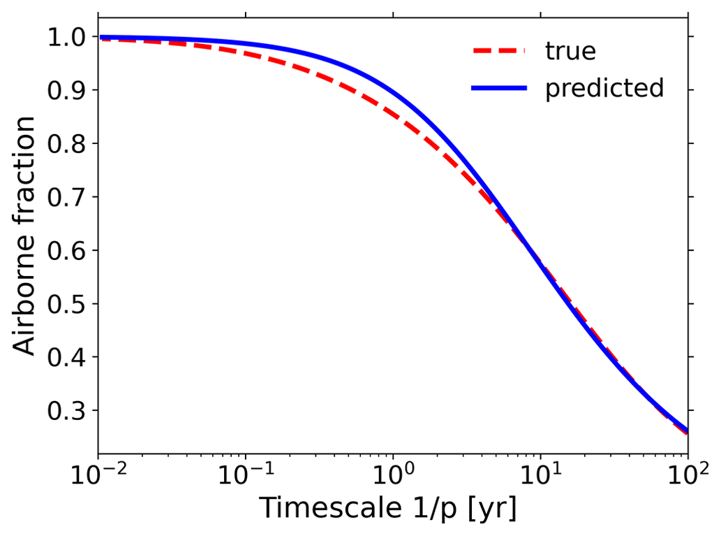
Figure 1 Quality of agreement between the true generalized airborne fraction (Eq. 18; see Sect. 3.1) and the generalized airborne fraction predicted by invoking Eq. (15) of the generalized α–β–γ framework (see Sect. 3.2). Technically, both curves were obtained by means of our RFI method from MPI simulation experiment data. But while the “predicted” curve is based on the generalized sensitivities derived from the usual pair of rad and bgc 1 % simulations using prescribed atmospheric CO₂ (concentration-driven), the “true” curve is based on data from impulse experiments performed with interactive CO₂ (emission-driven; see the detailed description in Appendix B). Note that the airborne fraction A plotted here differs from the standard airborne fraction AF (compare defining Eqs. 13 and 12) in that it is a scenario-independent generalization of it that predicts the response of atmospheric carbon accumulation rate to any weak emissions scenario (as demonstrated by Eqs. 13 in the time domain and 14 in the timescale domain). The maximum discrepancy between the two curves is around 5 % (1-year timescale). At timescales longer than 5 years, the average discrepancy is smaller than 1 %. The overall close agreement shows that the generalized α–β–γ framework gives – at least for MPI-ESM – a reasonable and scenario-independent description of the linear dynamics of the coupled climate–carbon system at global scale.

4 Timescale dependence of climate–carbon-cycle feedbacks and airborne fraction for weak perturbations in CMIP5 models

In the present section we extend our analysis of the timescale dependence of airborne fraction to the set of CMIP5 models listed in Table 1. In particular we study the importance of the different climate–carbon feedbacks for this timescale dependence.

Wu and Xin (2015b)Wu and Xin (2015c)Wu and Xin (2015d)Wu and Xin (2015a)Lindsay (2013b)Lindsay (2013c)Lindsay (2013d)Lindsay (2013a)Dunne et al. (2014a)Dunne et al. (2014b)Dunne et al. (2014c)Dunne et al. (2014d)Liddicoat et al. (2014a)Liddicoat et al. (2014b)Jones et al. (2014)Webb et al. (2014)IPSL (2011)IPSL (2011)IPSL (2011)Caubel et al. (2016)JAMSTEC et al. (2015b)JAMSTEC et al. (2015a)Torres Mendonca et al. (2023)Torres Mendonca et al. (2023)Torres Mendonca et al. (2023)Giorgetta et al. (2012)Tjiputra et al. (2012a)Tjiputra et al. (2012b)Bentsen et al. (2011)Tjiputra et al. (2012c)

Table 1 CMIP5 data considered in this study. For a description of the experiments please see Table A1.

The whole investigation is based on the calculation of the generalized airborne fraction by means of Eq. (15), whose power to predict airborne fraction from the generalized sensitivities has been demonstrated exemplarily for MPI-ESM in the previous section. As part of this demonstration, methods to derive the necessary generalized sensitivities from MPI-ESM standard C⁴MIP simulations had to be developed (see Appendix A). They are applied here to calculate also for those other CMIP5 models the generalized sensitivities from published 1 % bgc and 1 % rad simulation data.

4.1 Generalized sensitivities of CMIP5 models

In this subsection we present our results for the generalized sensitivities of the considered CMIP5 models. The robustness of the recovered sensitivities depends on the quality of the data (Torres Mendonça et al., 2021a, b) and on how appropriate it is to apply the numerical techniques selected in Appendix A for MPI-ESM to the other CMIP5 models as well. In principle this robustness should be examined for these other CMIP5 models by means of additional simulations, as was done for the MPI-ESM in Torres Mendonça et al. (2021b) and in Appendix A. But such simulations are not available. Nevertheless to get an idea of the quality of the recovered generalized sensitivities we use them to predict the time dependence of the standard α, β, and γ sensitivities for published 1 % simulations and compare them with their values obtained directly from the simulation data.

We start by discussing the identified generalized sensitivities. In Fig. 2 we show the ocean sensitivities in the first row and the land sensitivities in the second row. Figure 2a and d show the ${\mathit{\chi }}_{\mathit{\beta }}^{\left(\text{O}\right)}\left(t\right)$ and ${\mathit{\chi }}_{\mathit{\beta }}^{\left(\text{L}\right)}\left(t\right)$ sensitivities. The plotted vertical lines indicate the end of that part of the time series that is used to derive the sensitivities according to the techniques summarized in Table A2. As seen, these two sensitivities are for almost all models positive at all times analysed. This is because an increase in atmospheric CO₂ concentrations results in an increase in land and ocean carbon stocks: for land this positive response is a consequence of the CO₂ fertilization effect, which increases plant productivity and vegetation growth, while in the oceans it is a consequence of the increase in the difference between atmospheric and oceanic CO₂ partial pressure, leading to a positive input flux of CO₂ into the ocean (Arora et al., 2013; Friedlingstein et al., 2006). The surprising negative values of ${\mathit{\chi }}_{\mathit{\beta }}^{\left(\text{L}\right)}\left(t\right)$ for the HadGEM2-ES after 70 years are most likely a consequence of non-linearities in the response of this model: by the very nature of the biogeochemical response it can be shown that ${\mathit{\chi }}_{\mathit{\beta }}^{\left(\text{L}\right)}\left(t\right)$ should decrease monotonically to zero (see Torres Mendonça et al., 2021b, Appendix C), so the negative values must be an artefact of the numerical recovery caused either by the non-linearity of the response being stronger than expected from MPI-ESM or by deterioration from noise (Torres Mendonça et al., 2021a). Noting that the order of magnitude of the estimated signal-to-noise ratio in the HadGEM2-ES response is equal to or larger than that in the response of the other models (not shown), the negative values are most likely not caused by noise but are related to non-linearities. This result suggests that to reliably derive ${\mathit{\chi }}_{\mathit{\beta }}^{\left(\text{L}\right)}\left(t\right)$ for this model and to minimize the influence of non-linearities, one should take data until a perturbation strength smaller than that assumed following our investigation with MPI-ESM (Appendix A).

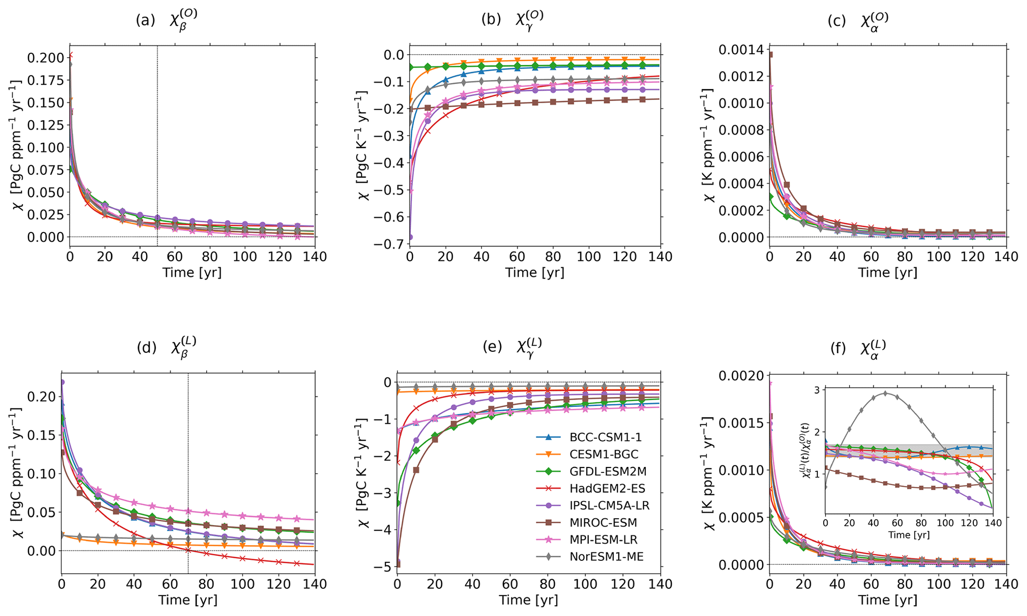
Figure 2 Generalized sensitivities (see definition in Eqs. 2–5) in CMIP5 models. All sensitivities were derived employing the RFI (response function identification) method (Torres Mendonça et al., 2021a) using the techniques selected in Appendix A (see summary Table A2). The inset in panel (f) shows the ratio of temperature sensitivities ${\mathit{\chi }}_{\mathit{\alpha }}^{\left(\text{L}\right)}\left(t\right)/{\mathit{\chi }}_{\mathit{\alpha }}^{\left(\text{O}\right)}\left(t\right)$, with the shaded area indicating the likely range of 1.4–1.7 for the ratio of land to ocean temperature (obtained for CMIP6 but consistent with CMIP5 estimates; Lee et al., 2021, Sect. 4.5.1.1.1; see discussion in text for more details). Changes with respect to pre-industrial equilibrium state were taken as $\mathrm{\Delta }x=x-x^{\mathrm{0}}$, where x⁰ is the mean value from the control simulation. Exceptions to this were ΔT_L and ΔT_O for MIROC-ESM: in the 1 % simulations from this model temperatures do not start at the level of pre-industrial equilibrium, so in this case we defined $\mathrm{\Delta }T=T-T^{\mathrm{0}}$ with T⁰:=T(0). The vertical lines in panels (a) and (d) indicate the time series length that was taken to derive the sensitivities; for the other plots the full time series was used.

There is a close agreement between the obtained generalized ocean sensitivities ${\mathit{\chi }}_{\mathit{\beta }}^{\left(\text{O}\right)}\left(t\right)$ in Fig. 2a: in most models ${\mathit{\chi }}_{\mathit{\beta }}^{\left(\text{O}\right)}\left(t\right)$ decays rapidly at a similar pace in the first years. Such overall agreement is in contrast to the results for the land sensitivities ${\mathit{\chi }}_{\mathit{\beta }}^{\left(\text{L}\right)}\left(t\right)$ in Fig. 2d, which spread largely for the different models. In particular the ${\mathit{\chi }}_{\mathit{\beta }}^{\left(\text{L}\right)}\left(t\right)$ sensitivities behave differently for the NorESM1-ME and CESM1-BGC models, which have very small values at all times. This behaviour may be explained by noting that these models account for the coupling between the nitrogen and carbon cycles, which reduces the strength of CO₂ fertilization because of nitrogen limitation (Zaehle et al., 2010; Arora et al., 2013). Excluding NorESM1-ME and CESM1-BGC, ${\mathit{\chi }}_{\mathit{\beta }}^{\left(\text{L}\right)}\left(t\right)$ for the other models agrees better at shorter than at longer times.

Figure 2b and e present the results for the ${\mathit{\chi }}_{\mathit{\gamma }}^{\left(\text{O}\right)}\left(t\right)$ and ${\mathit{\chi }}_{\mathit{\gamma }}^{\left(\text{L}\right)}\left(t\right)$ sensitivities. Both generalized sensitivities are negative for all times. This is because globally the land and ocean lose carbon to the atmosphere when only the climatic effect of CO₂ is taken into account. As clarified by Arora et al. (2013), this loss is explained by noting that rising temperatures over land result in an increase in heterotrophic soil respiration and almost everywhere to a decrease in net primary production (NPP), while over the oceans rising temperatures result primarily in a decrease in CO₂ solubility and thus degassing.

In contrast to ${\mathit{\chi }}_{\mathit{\beta }}^{\left(\text{O}\right)}\left(t\right)$, for ${\mathit{\chi }}_{\mathit{\gamma }}^{\left(\text{O}\right)}\left(t\right)$ the model spread is large over the whole time range (compare Fig. 2a and b). Particularly different is the behaviour of the sensitivities for MIROC-ESM and GFDL-ESM2M: while for all other models the magnitude of ${\mathit{\chi }}_{\mathit{\gamma }}^{\left(\text{O}\right)}\left(t\right)$ decreases rapidly in the first years, for these two models only a slow decrease resulting from strong contributions of long timescales in the generalized sensitivities (not shown) is observed. In fact the decrease is so slow that it looks as if they had constant values throughout the whole time range, but this is a misimpression induced by the scale of the plot.

The magnitude of ${\mathit{\chi }}_{\mathit{\gamma }}^{\left(\text{L}\right)}\left(t\right)$ is – at least at short times – much larger than that of ${\mathit{\chi }}_{\mathit{\gamma }}^{\left(\text{O}\right)}\left(t\right)$ for almost all models except for NorESM1-ME and CESM1-BGC. As explained by Arora et al. (2013), in these two models the coupling between the nitrogen and carbon cycles weakens not only the biogeochemical but also the radiative response because temperature-driven nitrogen remineralization enhances plant productivity, which counteracts the parallel carbon loss from the enhanced soil respiration in the warmer climate (see also Melillo et al., 2002; Thornton et al., 2009). Analogously to ${\mathit{\chi }}_{\mathit{\gamma }}^{\left(\text{O}\right)}\left(t\right)$ in MIROC-ESM and GFDL-ESM2M, because of strong contributions from long timescales, the generalized sensitivity ${\mathit{\chi }}_{\mathit{\gamma }}^{\left(\text{L}\right)}\left(t\right)$ decays in the two other models NorESM1-ME and CESM1-BGC so slowly (see Fig. 2e) that it seems as if it had a constant value throughout the time series, which is also only a misimpression due to the scale. Overall there is a better model agreement for ${\mathit{\chi }}_{\mathit{\gamma }}^{\left(\text{L}\right)}\left(t\right)$ at long rather than at short times.

Finally, Fig. 2c and f present the results for the ${\mathit{\chi }}_{\mathit{\alpha }}^{\left(\text{O}\right)}\left(t\right)$ and ${\mathit{\chi }}_{\mathit{\alpha }}^{\left(\text{L}\right)}\left(t\right)$ sensitivities that characterize the response of ocean and land temperature to atmospheric CO₂ perturbations. For both ${\mathit{\chi }}_{\mathit{\alpha }}^{\left(\text{O}\right)}\left(t\right)$ and ${\mathit{\chi }}_{\mathit{\alpha }}^{\left(\text{L}\right)}\left(t\right)$ there is a relatively good agreement among models. A larger spread is nevertheless found for values at short times, for which the recovery is less robust due to ill-posedness of the deconvolution problem that must be solved to recover the generalized sensitivities (Torres Mendonça et al., 2021a). We note also that the values of both sensitivities are closely related: this is expected from the well-known fact that by various mechanisms the ratio $\mathrm{\Delta }{T}_{\text{L}}/\mathrm{\Delta }{T}_{\text{O}}=:a$ of land to ocean temperature is around 1.4–1.7 (Lee et al., 2021, Sect. 4.5.1.1.1; Eyring et al., 2021, Fig. 3.2b). By their definition in the Laplace domain ${\stackrel{\mathrm{̃}}{\mathit{\chi }}}_{\mathit{\alpha }}^{\left(\text{O}\right)}\left(p\right)=\mathrm{\Delta }{\stackrel{\mathrm{̃}}{T}}_{\text{O}}\left(p\right)/\mathrm{\Delta }\stackrel{\mathrm{̃}}{c}\left(p\right)$ and ${\stackrel{\mathrm{̃}}{\mathit{\chi }}}_{\mathit{\alpha }}^{\left(\text{L}\right)}\left(p\right)=\mathrm{\Delta }{\stackrel{\mathrm{̃}}{T}}_{\text{L}}\left(p\right)/\mathrm{\Delta }\stackrel{\mathrm{̃}}{c}\left(p\right)$, it follows that ${\stackrel{\mathrm{̃}}{\mathit{\chi }}}_{\mathit{\alpha }}^{\left(\text{L}\right)}\left(p\right)=a\mathrm{\Delta }{\stackrel{\mathrm{̃}}{T}}_{\text{O}}\left(p\right)/\mathrm{\Delta }\stackrel{\mathrm{̃}}{c}\left(p\right)=a{\stackrel{\mathrm{̃}}{\mathit{\chi }}}_{\mathit{\alpha }}^{\left(\text{O}\right)}\left(p\right)$ so that these two generalized sensitivities should differ by about that factor. Interestingly, this is indeed seen for most models (see inset in Fig. 2f) but only for the first decades – over the last years a large spread arises.

We now turn to the analysis of the plausibility of the recovered generalized sensitivities by means of the prediction of the original α, β, and γ sensitivities for standard C⁴MIP 1 % simulations. For this analysis we first employ the recovered generalized sensitivities to predict the original α, β, and γ sensitivities and then compare the results to the actual α, β, and γ sensitivities obtained directly from data. That the original α, β, and γ sensitivities can in principle be predicted from the generalized sensitivities may be seen by noting that

$$\begin{array}{}\text{(20)}& {\displaystyle }{\mathit{\beta }}^{\left(X\right)}\left(t\right):={\displaystyle \frac{\mathrm{\Delta }{C}_X^{\text{bgc}}\left(t\right)}{\mathrm{\Delta }c\left(t\right)}}={\displaystyle \frac{\mathrm{1}}{\mathrm{\Delta }c\left(t\right)}}\underset{\mathrm{0}}{\overset{t}{\int }}{\mathit{\chi }}_{\mathit{\beta }}^{\left(X\right)}(t-s)\mathrm{\Delta }c\left(s\right)\mathrm{d}s,\text{(21)}& {\displaystyle }\begin{array}{rl}{\mathit{\gamma }}^{\left(X\right)}\left(t\right):& ={\displaystyle \frac{\mathrm{\Delta }{C}_X^{\text{rad}}\left(t\right)}{\mathrm{\Delta }{T}_X^{\text{rad}}\left(t\right)}}={\displaystyle \frac{\mathrm{1}}{\mathrm{\Delta }{T}_X^{\text{rad}}\left(t\right)}}\underset{\mathrm{0}}{\overset{t}{\int }}{\mathit{\chi }}_{\mathit{\gamma }}^{\left(X\right)}(t-s)\\ & \mathrm{\Delta }{T}_X^{\text{rad}}\left(s\right)\mathrm{d}s,\end{array}\text{(22)}& {\displaystyle }{\mathit{\alpha }}^{\left(X\right)}\left(t\right):={\displaystyle \frac{\mathrm{\Delta }{T}_X^{\text{rad}}\left(t\right)}{\mathrm{\Delta }c\left(t\right)}}={\displaystyle \frac{\mathrm{1}}{\mathrm{\Delta }c\left(t\right)}}\underset{\mathrm{0}}{\overset{t}{\int }}{\mathit{\chi }}_{\mathit{\alpha }}^{\left(X\right)}(t-s)\mathrm{\Delta }c\left(s\right)\mathrm{d}s,\end{array}$$

where X stands for land (L) or ocean (O), the superscripts “bgc” and “rad” indicate data taken from bgc and rad simulations (see Table A1), and quantities pre-fixed by Δ stand for a difference with respect to pre-industrial times. The first equalities are the definitions of the standard α, β, and γ sensitivities (Friedlingstein et al., 2003). The second equalities are obtained by inserting Eqs. (2)–(5) while accounting for the specific setup of the bgc and rad simulations: to a good approximation (Friedlingstein et al., 2003) temperature remains unchanged in the bgc simulations, while the CO₂ rise acts only via climate on land and ocean carbon storage in the rad simulations. In the following analysis we compare the prediction from the generalized sensitivities (second equalities) to the actual α, β, and γ values computed by their definition directly from the simulation data (first equalities). The whole comparison is performed for the 1 % rad and the 1 % bgc simulations (Table A1).

The results of these calculations are shown in Fig. 3. We plot the α, β, and γ sensitivities as a function of time for the first 30 years of the 1 % simulations so that CO₂ forcing strengths are within the estimated linear regime of the generalized framework (around 94 ppm; see Appendix A). Because of natural climate variability there is some uncertainty in the choice of the values of pre-industrial temperature and carbon stocks needed to calculate the differences ΔT_X(t) and ΔC_X(t) in the definitions of the sensitivities (see Eqs. 20–22). In Fig. 3 we used the variability from the associated control simulations to estimate the resulting uncertainty range for the data-derived sensitivities (shaded area in the figures) – details are found in Appendix E. As seen in the figure, for γ(t) the uncertainty range sometimes gets extremely large; this happens when the ΔT_X(t) found in the denominator comes close to zero (see Eq. E5). In principle, such an uncertainty from initial values enters also the denominator of the predicted γ sensitivities, but we do not display this to keep the figures simple, and the interpretation of this comparison would not change.

The results for MPI-ESM-LR can be considered a reference for the achievable agreement between data-derived and predicted sensitivities because for MPI-ESM-LR the generalized sensitivities were obtained in a quality-controlled way by means of additional simulations (see Appendix A) not available for the other models. In view of this achievable agreement, the predicted α and γ sensitivities excellently match for all models the respective data-derived sensitivities, judged by noting that the predicted sensitivities stay within the amplitude range of inter-annual variability that is by principle not predictable by the linear response methods employed here because they predict the ensemble mean instead of the individual system development (see the discussion in Torres Mendonça et al., 2021a). In contrast, for all models the predicted β^(O)(t) is – for times longer than 15 years – systematically too high. Additionally, the predicted β^(L)(t) has a slope and/or offset that systematically differs from those of the respective data-derived β^(L)(t).

Such systematic deviations in β^(O)(t) and β^(L)(t) are largely a result of the effect of non-linearities in the respective carbon responses $\mathrm{\Delta }{C}_X^{\text{bgc}}\left(t\right)$: in fact, if the predicted sensitivities are calculated by using not the untransformed forcing Δc(t) under the integral in Eq. (20) but rather the transformed forcings $c_{\text{PI}}\ln \left(c\right(t)/c_{\text{PI}})$ and ΔNPP(t) – these are used in the derivation of the generalized sensitivities ${\mathit{\chi }}_{\mathit{\beta }}^{\left(X\right)}$ to account for non-linearities (see Appendices A2 and A5) – the quality of agreement for β^(O)(t) and β^(L)(t) considerably improves (not shown). We nevertheless chose to perform the predictions with the untransformed forcing Δc(t) to conform with the standard formulation of the generalized framework (compare Eqs. 2–5). Despite the encountered deviations in β^(X)(t), in all cases the magnitude and tendency of the predicted sensitivities match those of the data-derived sensitivities.

Overall, we consider the results of this comparison as sufficiently convincing to add confidence to the validity of the recovered generalized sensitivities (Fig. 2) that underlie the predicted α, β, and γ sensitivities in Fig. 3. We note also that the predicted sensitivities, in contrast to the often noisy data-derived sensitivities, are typically well defined because, as mentioned above, the generalized sensitivities predict the response not in noisy individual realizations but in a smooth ensemble mean. Nevertheless, it should be kept in mind that this comparison is a mere plausibility check because essentially the same data used to predict the α, β, and γ sensitivities were also used to derive the generalized sensitivities.

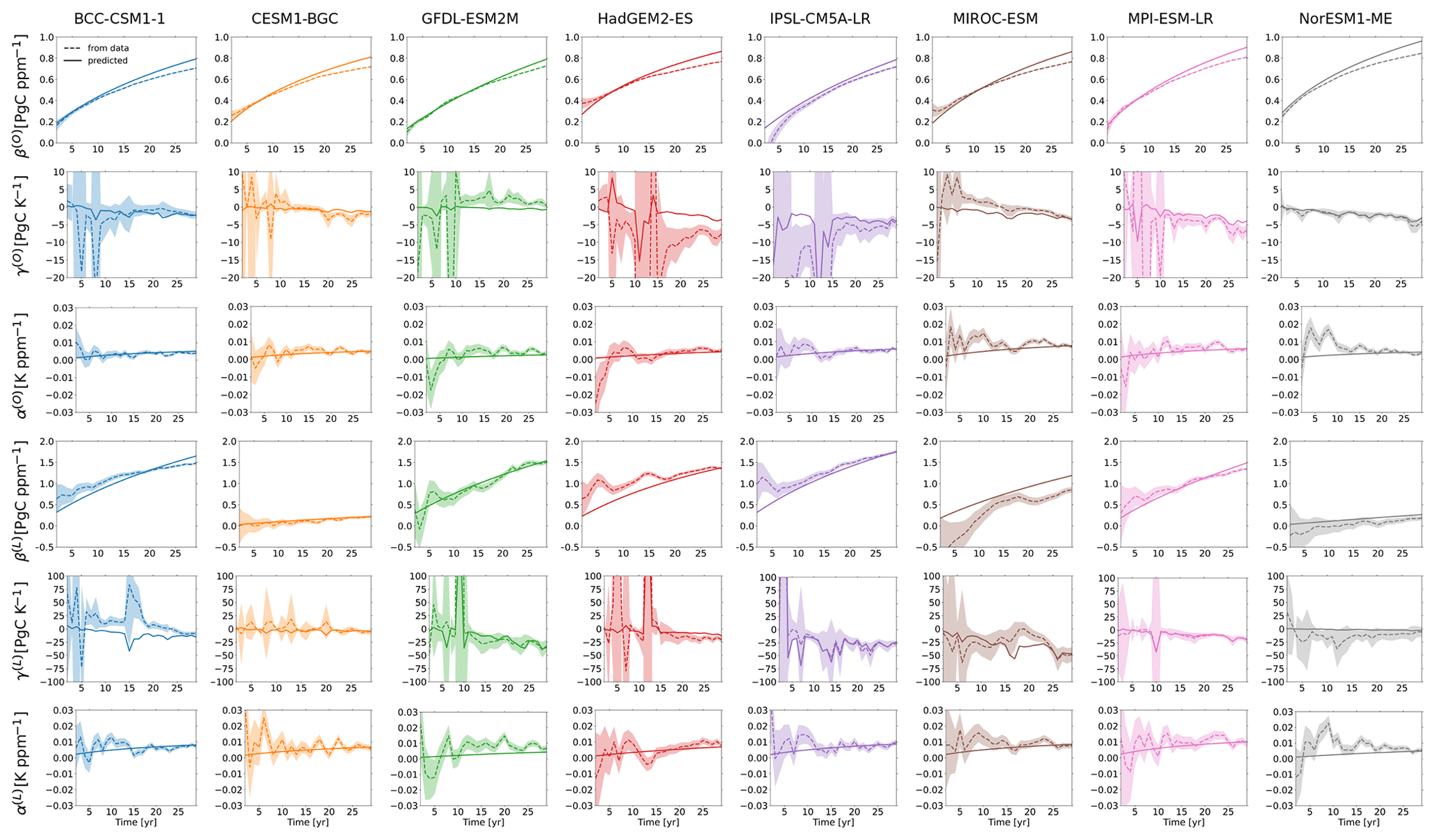
Figure 3 The α, β, and γ sensitivities calculated directly via first equalities of Eqs. (20)–(22) from the simulation data (dashed lines) and predicted via second equalities of Eqs. (20)–(22) from the generalized sensitivities (solid lines). The plots are restricted to the first 3 decades of the simulations (equivalent to about 94 ppm CO₂ rise), where all responses are expected to be linear (see Table A2). Uncertainty ranges are calculated taking into account uncertainty in the choice of the initial value (see Appendix E).

4.2 Additivity of responses

Before the main question of this study on the role of feedbacks for airborne fraction can finally be addressed in the next section, another preparatory step is necessary. Key to investigate this question will be Eq. (15) from the generalized framework to predict the generalized airborne fraction via the feedback functions from the generalized sensitivities as already explained in Sect. 3.2. In applying this relation to the data from the different CMIP5 models one must realize that the accuracy of such predictions depends on two aspects: (1) the quality of the numerical recovery of the generalized sensitivities (see previous subsection) and (2) the validity of the assumption underlying the generalized framework that for weak perturbations the carbon response to CO₂ is determined by the sum of the biogeochemical and radiative responses; this assumption of additivity is implicit to Eqs. (2)–(3), where the first term represents the biogeochemical response and the second (after insertion of Eqs. 4–5) the radiative response. Ideally, for each model one should fully check these two aspects with the aid of additional simulations, as we did for the MPI-ESM in Torres Mendonça et al. (2021b) and in Appendix A. Unfortunately, such additional simulations are at present not available for other models, so a full check is not possible. Nevertheless, since all CMIP5 models provide in addition to the 1 % rad and bgc simulations also a 1 % fully coupled simulation (a 1 % simulation where both the biogeochemical and the radiative effects of CO₂ are active), one can at least check whether the biogeochemical and radiative responses are indeed additive for a certain range of perturbation strengths. The rationale underlying this check is that the 1 % rad and bgc simulations separately give the values for the two right-hand-side terms in Eqs. (2)–(3), while the 1 % fully coupled simulation gives the left-hand sides.

To check additivity, we plot in Fig. 4 for each of these models the response in carbon storage for land, ocean, and global (land plus ocean) carbon from the 1 % fully coupled experiment along with the sum of the responses from the 1 % bgc and 1 % rad experiments. If additivity holds for a certain range of perturbation strengths, then within this range these two curves (1 % fully coupled and the sum of 1 % bgc and 1 % rad) must agree. As seen, for all models there is indeed agreement at least within the estimated range of linearity (94 ppm CO₂ rise; see Appendix A) for land, ocean, and global carbon stock changes, with larger discrepancies for land and global carbon in MIROC-ESM and NorESM1-ME. For those two models, the generalized framework may not fully describe the linear dynamics of the system in the fully coupled setup. But overall, within the linear regime one may say that the biogeochemical and radiative responses are approximately additive in the CMIP5 models. This result, together with the evidence for the overall plausibility of the generalized sensitivities obtained in the last subsection, gives some confidence that our numerical methods and the framework as a whole are describing in reasonable approximation the linear dynamics of the carbon cycle in these models.

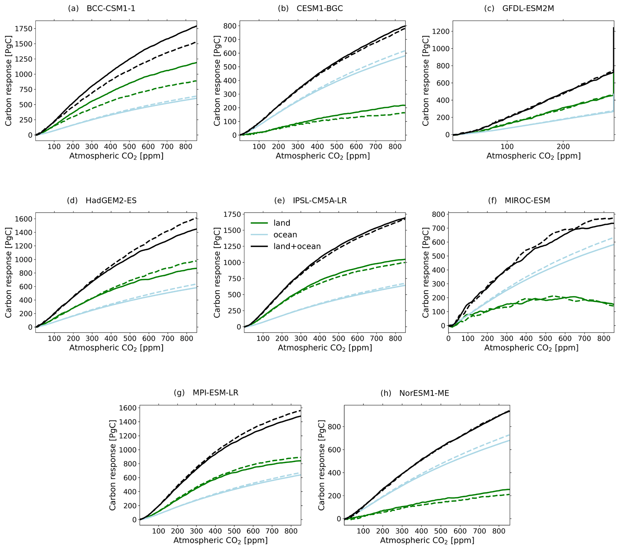
Figure 4 Check of the additivity of the biogeochemical and radiative carbon responses in CMIP5 models that underlies the generalized α–β–γ-framework (compare Eqs. 2–3). Plotted are the sum of the responses from the 1 % bgc and 1 % rad experiments (dashed lines) and the response from the 1 % fully coupled experiment (solid lines) for land (green), ocean (blue), and global carbon (land plus ocean; black). Note that in contrast to all other simulations, for GFDL-ESM2M the prescribed atmospheric CO₂ increase by 1 % per year does not last for the full 140 years but only for the first 70 years, from which CO₂ is kept at the level reached. This explains the peculiar vertical behaviour at the end of the time series in panel (c); while CO₂ is held constant (note the reduced CO₂ scale), carbon stocks continue accumulating on land and in the ocean. This figure confirms that additivity holds approximately within the estimated linear regime of 94 ppm (see Appendix A) for all models. For more details see text.

4.3 Climate–carbon-cycle feedbacks and airborne fraction

In this section we tackle the main question of our study, namely how the climate–carbon-cycle feedbacks shape the timescale dependence of the generalized airborne fraction. From here on we take for granted that by the methods presented in the previous sections Eq. (15) indeed reliably predicts the generalized airborne fraction for the considered CMIP5 models. We thus proceed to estimate the feedbacks and the airborne fraction for each model via Eqs. (9), (10), and (15). The results are shown in Fig. 5.

In Fig. 5a, one sees that for almost all CMIP5 models the timescale-dependent airborne fraction decreases as the timescale $\mathrm{1}/p$ increases, all starting at 1 for short timescales and spreading from 0.56 to 0.75 at a timescale of 10 years and from 0.26 to 0.5 at a timescale of 100 years. The only exception is HadGEM2-ES, whose timescale-dependent airborne fraction once more increases at long timescales, which, as will be seen below, is related to a reduction in the magnitude of its land biogeochemical feedback. That the airborne fraction has a value of 1 at short timescales is not a property of the models but follows from its definition (compare Eq. 19). But this is not so for the decrease in airborne fraction at long timescales: as will become clear below this behaviour is a consequence of the biogeochemical feedback being stronger than the radiative feedback in the considered CMIP5 models, so this decrease is presumably a genuine property of the Earth system.

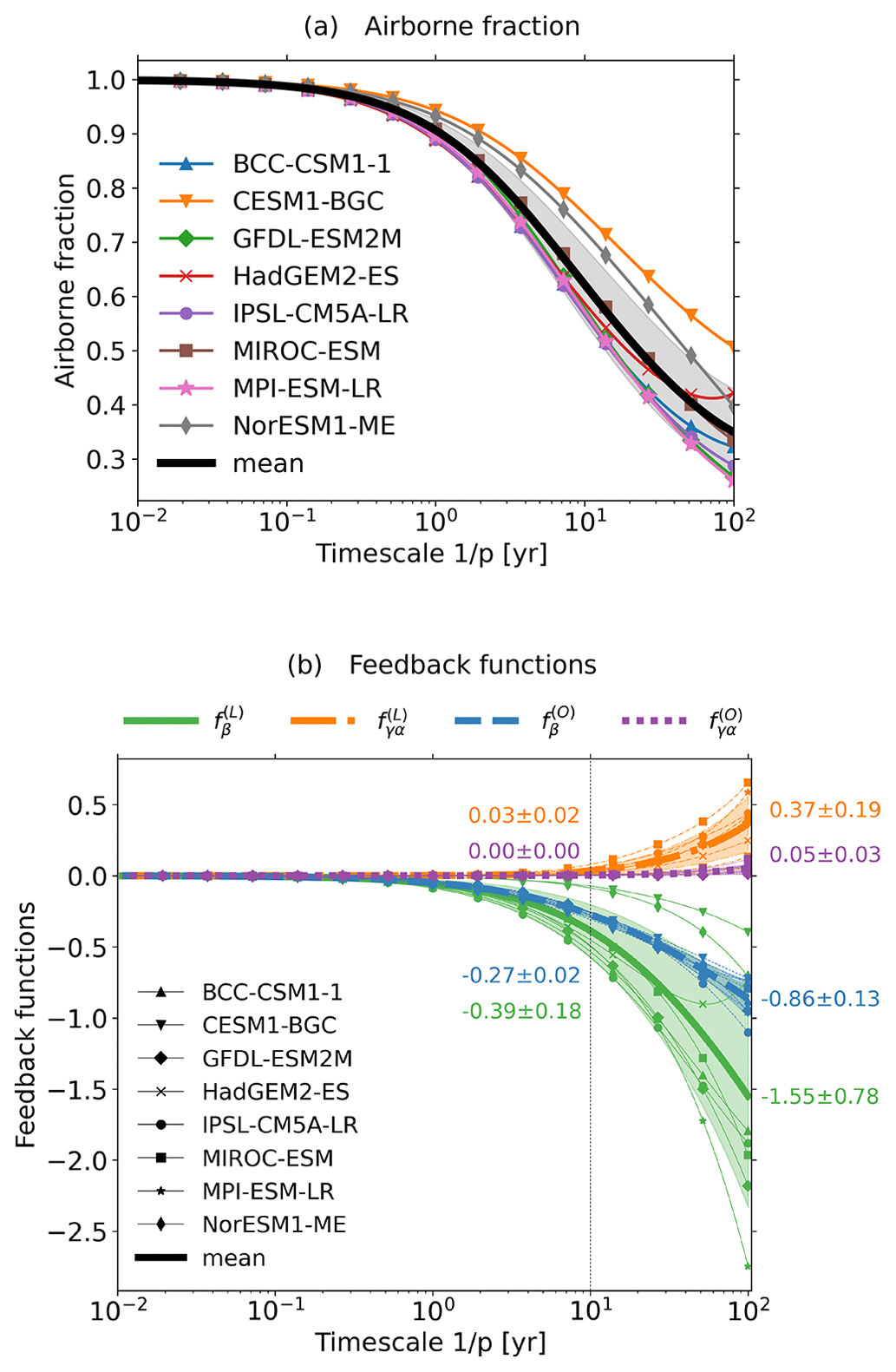
Figure 5 Airborne fraction and climate–carbon-cycle feedbacks in CMIP5 models as derived by the generalized framework (Eqs. 15, 9, and 10). The numbers in panel (b) indicate the model mean and standard deviation for each feedback function at 10-year and 100-year timescales. Note that the generalized airborne fraction and all feedback functions are dimensionless.

How the airborne fraction changes in the timescale domain is determined by the climate–carbon-cycle feedbacks. As seen in Fig. 5b, for $\mathrm{1}/p\to \mathrm{0}$ all feedback functions approach zero, which in view of Eq. (15) is consistent with $\stackrel{\mathrm{̃}}{A}\left(p\right)\to \mathrm{1}$ for the airborne fraction. Besides the mathematical reasons explained in connection with Eq. (19), this behaviour can intuitively be understood by noting that at short timescales the ocean and land carbon cycles have not yet reacted to emissions, so at these scales $\stackrel{\mathrm{̃}}{A}\left(p\right)\to \mathrm{1}$ and thus atmospheric CO₂ simply follows emissions (Eq. 14). To understand how the airborne fraction behaves as the timescale increases, one must look at the behaviour of the separate feedback functions. For longer timescales, the feedback functions ${\stackrel{\mathrm{̃}}{f}}_{\mathit{\gamma }\mathit{\alpha }}^{\left(\text{L}\right)}$ and ${\stackrel{\mathrm{̃}}{f}}_{\mathit{\gamma }\mathit{\alpha }}^{\left(\text{O}\right)}$ that quantify the radiative feedbacks become increasingly positive, while the feedback functions ${\stackrel{\mathrm{̃}}{f}}_{\mathit{\beta }}^{\left(\text{L}\right)}$ and ${\stackrel{\mathrm{̃}}{f}}_{\mathit{\beta }}^{\left(\text{O}\right)}$ that quantify the biogeochemical feedbacks become in general increasingly negative. The sign of these feedbacks is in agreement with current process understanding (Friedlingstein et al., 2006; Gregory et al., 2009; Arora et al., 2013, 2020). But that these feedbacks are either positive or negative for all timescales is a non-trivial result that could not be obtained by the original α–β–γ framework because there the timescale-dependent feedback strengths show up only combined with the external forcing that enters the quantification by the underlying α, β, and γ sensitivities (see discussion in Sect. 2). The observed uniformity of the sign of the feedbacks is explained by the fact that almost all generalized sensitivities in Fig. 2 are either always negative or always positive: since the feedback functions are proportional either to the Laplace transform of χ_β or to the product of the Laplace transforms of χ_γ and χ_α (Eqs. 9 and 10), one sees following the lines of the argument for $\stackrel{\mathrm{̃}}{A}\left(p\right)\ge \mathrm{0}$ in Appendix D that by the positivity or negativity of these response functions in time also their Laplace transforms and the associated feedback functions must have a unique sign at all timescales. Interestingly, for increasing timescales in almost all models – except for the HadGEM2-ES at long timescales – the sum (land plus ocean) of the biogeochemical feedbacks becomes increasingly larger than the sum of the radiative feedbacks. As a result, in all these models the total feedback function $\stackrel{\mathrm{̃}}{f}\left(p\right)$ gets increasingly negative (not shown) and by Eq. (15) the airborne fraction always decreases. In the HadGEM2-ES, at long timescales the magnitude of the land biogeochemical feedback starts to decrease, thereby reducing the magnitude of the (negative) total feedback function and as a consequence increasing the airborne fraction.

In the mean over all models, the land biogeochemical feedback is at all timescales longer than the ocean biogeochemical feedback: at a timescale of 10 years, it is 1.4 times larger, and at a timescale of 100 years, it is 1.8 times larger. The picture is qualitatively similar for the radiative feedback: at a timescale of 10 years, the land feedback is, despite its small value of 0.03, orders of magnitude larger than the almost absent ocean feedback, and at a timescale of 100 years, the land feedback is 7.4 times larger than its ocean counterpart. Aggregating land and ocean, the mean of the biogeochemical feedback is 22 times larger than the radiative feedback at a timescale of 10 years and 5.6 times larger at a timescale of 100 years. These results are in particular at short timescales in contrast to previous estimates (Gregory et al., 2009; Arora et al., 2013) using Friedlingstein's framework, which suggested that the biogeochemical feedback is about 4 times larger than the radiative feedback. One must note though that our and previous estimates are not entirely comparable: while previous estimates were made for a particular scenario, our estimate is valid for any scenario. In addition, here only the linear regime is considered, so the saturation of the land and ocean carbon sinks (which reduces the values of β^(L) and β^(O) when higher perturbation strengths are considered) is not taken into account.

By Fig. 5b the model spread is for the land feedbacks much larger than that for the ocean feedbacks, as expected from previous studies (Gregory et al., 2009; Arora et al., 2013; Friedlingstein et al., 2014). Because of the non-linear relationship between $\stackrel{\mathrm{̃}}{A}\left(p\right)$ and the feedback functions (see Eq. 15), it is not immediately clear how the model spread in the feedbacks propagates to the airborne fraction. Assuming small, independent spreads, this propagation may be computed as

$$\begin{array}{}\text{(23)}& \begin{array}{rl}{\mathit{\sigma }}_A^{\mathrm{2}}& \left(p\right)\approx {\stackrel{\mathrm{̃}}{A}}^{\mathrm{4}}\left(p\right)\left({\mathit{\sigma }}_{f_{\mathit{\beta }}^{\left(\text{L}\right)}}^{\mathrm{2}}\right(p)+{\mathit{\sigma }}_{f_{\mathit{\gamma }\mathit{\alpha }}^{\left(\text{L}\right)}}^{\mathrm{2}}(p)+{\mathit{\sigma }}_{f_{\mathit{\beta }}^{\left(\text{O}\right)}}^{\mathrm{2}}(p)\\ & +{\mathit{\sigma }}_{f_{\mathit{\gamma }\mathit{\alpha }}^{\left(\text{O}\right)}}^{\mathrm{2}}\left(p\right)),\end{array}\end{array}$$

where σ² denotes the spread (variance) for each quantity. This follows by expanding $\stackrel{\mathrm{̃}}{A}\left(p\right)$ around the mean into the feedback functions, assuming small spreads in the functions so that only linear terms are kept, and then calculating the variance of the result assuming independent spreads so that covariance terms are ignored (Roe, 2009; Barlow, 1989, p. 55). Figure 6a shows the terms on the right-hand side of Eq. (23), the resulting approximation of ${\mathit{\sigma }}_{\stackrel{\mathrm{̃}}{A}}^{\mathrm{2}}\left(p\right)$ (sum of those terms), and the true spread in the airborne fraction. As seen, the true variance in the airborne fraction follows closely the component arising from the land biogeochemical feedback, with a slightly larger discrepancy at timescales above 30 years, indicating that on longer timescales other feedbacks' spread becomes relatively more important. This indicates that most of the model spread in the airborne fraction arises from the spread in the land biogeochemical feedback. This result agrees with that obtained in a recent study (Jones and Friedlingstein, 2020) that also evaluated how the model spread in the airborne fraction is affected by the spread in the climate–carbon-cycle feedbacks but employing Friedlingstein's original framework for the analysis.

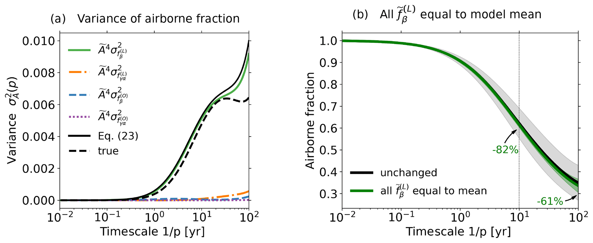
Figure 6 Analysis of model spread of feedback functions and their influence on the airborne fraction. (a) Spread (variance) of airborne fraction and decomposition in terms of the feedback contributions according to Eq. (23); (b) airborne fraction (averaged over all models) and its model spread (standard deviation) as shown in Fig. 5a (unchanged) and airborne fraction and the model spread that one would obtain if the feedback function ${\stackrel{\mathrm{̃}}{f}}_{\mathit{\beta }}^{\left(\text{L}\right)}$ was for all models equal to the model mean. Percentages in (b) indicate the reduction in the airborne fraction model spread compared to the true spread at 10- and 100-year timescales. See text for more details.

An even clearer view about the impact of the different feedbacks on the airborne fraction may be gained by artificially changing the values of these feedbacks to study hypothetical situations and then evaluating the resulting change in the airborne fraction. For instance, one can illustrate how strongly the model spread in the airborne fraction depends on the spread in the land biogeochemical feedback by recalculating the statistics of the airborne fraction taking ${\stackrel{\mathrm{̃}}{f}}_{\mathit{\beta }}^{\left(\text{L}\right)}$ for all models equal to its model mean. As shown in Fig. 6b, it turns out that if the exact values of only this feedback function were known and equal to the model mean (with all other feedback spreads remaining the same), the spread in the airborne fraction would reduce by about 82 % at a timescale of 10 years and 61 % at a timescale of 100 years. This once more makes obvious that the main reason for the model spread in the airborne fraction is the large spread in the land biogeochemical feedback.

5 Conclusions

The dynamics of the global carbon cycle can be understood in terms of feedbacks arising via the land and ocean carbon cycle when atmospheric CO₂ is perturbed. To disentangle and separately quantify those feedbacks, Friedlingstein et al. (2003) developed the α–β–γ framework. Although this framework gives insight into the main effects of atmospheric CO₂ perturbations in the global carbon cycle, by not accounting for the internal timescales of the system, the resulting quantification of feedbacks is valid only for a particular perturbation scenario and time period. Such limitations are overcome by employing the recently proposed generalization of this framework (Heimann, 2014; Rubino et al., 2016; Enting and Clisby, 2019; Enting, 2022). By assuming weak perturbations and accounting for the memory of the carbon cycle, the generalized α–β–γ framework quantifies feedbacks independently of the perturbation scenario at different timescales. As a result of the generalization, this framework gives in principle a complete description of the linear dynamics of the global carbon cycle in terms of the underlying feedbacks. But so far its applicability to study the dynamics of the climate–carbon system had not been systematically investigated.

Here, we employed this generalized framework to study the timescale dependence of the climate–carbon-cycle feedbacks and the associated airborne fraction for an ensemble of CMIP5 models. In Sect. 3, we have shown for the example of MPI-ESM that the generalized sensitivities identified from concentration-driven simulations correctly predict via Eqs. (7)–(8) and (15) the generalized airborne fraction derived from emission-driven simulations. This demonstrates that the generalized α–β–γ framework has indeed predictive power.

Based on experience with MPI-ESM, we quantified in Sect. 4 the timescale-dependent airborne fraction and feedbacks for various other CMIP5 models. As can be seen from Eq. (14), the timescale-dependent airborne fraction quantifies the fraction of emissions staying in the atmosphere at a particular timescale. At short timescales this fraction is known to be 1; i.e. atmospheric carbon simply follows emissions because feedbacks that could change it need sufficient time to react. We found that for almost all models, the airborne fraction strictly decreases towards long timescales. This decrease is slow: even at a timescale of 100 years the airborne fraction has dropped down only to values ranging from 0.26 to 0.5, meaning that even a century after CO₂ emissions happened a considerable amount is still airborne, which is consistent with results from impulse experiments (Archer et al., 2009).

Considering global carbon, in the model mean the biogeochemical feedback was found to be 22 times larger than the radiative feedback at a 10-year timescale and 5.6 times larger at a 100-year timescale. This result suggests that at least over shorter timescales the difference between these feedbacks may be even greater than previously thought (Gregory et al., 2009; Arora et al., 2013). Nevertheless, one must note that here only the linear perturbation regime is considered, so a possible saturation of the land and ocean carbon sinks at high CO₂ (that would reduce the values of β^(L) and β^(O) compared to the case where no saturation is present) is not reached.

The influence of the model spread of the different feedbacks on the airborne fraction was also investigated. It was found that the spread in the airborne fraction arises mostly from the spread in the land biogeochemical feedback, especially for timescales below 30 years. By considering the hypothetical case where this particular feedback would be equal to the model mean, we found that the spread in the airborne fraction would decrease by 82 % at a 10-year timescale and by 61 % at a 100-year timescale, which demonstrates even more clearly that it is indeed the land biogeochemical feedback that causes the spread in airborne fraction between the different models.

6 Discussion

While the generalized framework was shown here to reasonably describe the linear dynamics of the global carbon cycle in MPI-ESM, the results obtained for the other CMIP5 models depend on two basic assumptions. The first is that the generalized sensitivities in the CMIP5 models are recoverable with sufficient quality by the same numerical approaches that were appropriate to recover the sensitivities in MPI-ESM. This involves the assumption that for all other considered CMIP5 models the linear perturbation regime is of similar extent to that found for MPI-ESM for the different response variables invoked to recover the sensitivities. This might not be the case – and is probably not for ${\mathit{\chi }}_{\mathit{\beta }}^{\left(\text{L}\right)}$ in the HadGEM2-ES (see discussion of Fig. 2d). The second basic assumption is that the generalized framework itself correctly describes the dynamics of the global carbon cycle in those models. This involves the assumption that the biogeochemical and radiative responses are additive – which was confirmed to a good degree of approximation within the linear regime (see Fig. 4) – but also that the whole carbon cycle dynamics can be described in terms of the responses to atmospheric CO₂ and temperature alone (see Eqs. 2–5). Ideally, each of these assumptions should be carefully investigated for each model separately by aid of additional simulations, similarly to what was done here for the case of MPI-ESM.

With these cautionary remarks in mind, our conclusion that the spread in the airborne fraction arises mostly from the spread in the land biogeochemical feedback corroborates the recent finding by Jones and Friedlingstein (2020), who performed a similar analysis employing Friedlingstein's original α–β–γ framework. This agreement adds confidence to the results obtained here and suggests that research on climate–carbon-cycle feedbacks should focus especially on understanding the land biogeochemical feedback, since it is the largest source of model uncertainty in the airborne fraction in our and in their analysis. But additionally, the conclusion drawn here is valid not only for the particular perturbation scenario underlying the CMIP5 protocol but for all scenarios within the linear regime. To this extent, this study at least partially answers the question raised by Jones and Friedlingstein (2020) about the behaviour of climate–carbon-cycle feedbacks in scenarios with different characteristics: as long as we stay within the linear regime, there is no need for calculating separate feedback metrics for the different scenarios; the feedback functions of the generalized framework describe this behaviour for all scenarios at once.

Estimates of the timescale-resolved airborne fraction, by means of Eq. (18), and of timescale-dependent generalized sensitivities had already been attempted (Enting, 2007, 2022; Rubino et al., 2016; Enting and Clisby, 2019). These attempts, focused on the observed carbon cycle, were based on ad hoc assumptions on the internal memory in terms of the analytical structure of the underlying response functions and values of internal timescales. Such assumptions could be circumvented in the present study by employing our RFI method (Torres Mendonça et al., 2021a, b) that instead derives the internal timescale spectra of the system by fully accounting for the ill-posedness of the underlying inverse problem. But it should be noted that our approach is tailored to simulation data, and whether it may be applicable to observation data needs to be seen. One of the involved challenges for such an application is that our setting here is limited to an idealized case where CO₂ is the only forcing, while in observations one would have to account for further perturbations such as non-CO₂ greenhouse gases, land use change, and aerosols.

As explained in Sect. 2, the timescale-resolved airborne fraction can be understood as a generalization of the airborne fraction in its standard definition (defined as a ratio of atmospheric CO₂ fluxes to emission fluxes; see Eq. 12). It is well known that the near-constancy of the value of the standard airborne fraction is a result of the linearity of response in combination with the exponential character of the increase in historic emissions (Raupach, 2013). Accordingly, once emissions get non-exponential – as it must be if future emissions are significantly reduced – the standard airborne fraction must deviate from its constant value (Raupach, 2013). Thus, standard airborne fraction cannot be seen as an invariant property of the climate–carbon system. In contrast, the generalized airborne fraction investigated here describes the response of atmospheric CO₂ to any emissions scenario and is therefore indeed an invariant property of the system. As such, the generalized airborne fraction may be employed to predict the standard airborne fraction by Eq. (13) for any emissions scenario as long as emissions are sufficiently weak (see Appendix F for an exemplary demonstration). This is the case, for example, for emission scenarios with low or even negative future emissions, as investigated in Jones et al. (2016). For such scenarios the generalized airborne fraction – once it has been determined for one or more models – could be used as an emulator to see without expensive Earth system simulations how atmospheric CO₂ develops; and a similar approach could be applied to changes in the land and ocean carbon reservoirs by determining the appropriate response functions.

7 Outlook

Besides investigating the timescale dependence of airborne fraction, our study also demonstrated for MPI-ESM the predictive power of the generalized framework (see Sect. 3). This demonstration indicates that this framework may be invoked also to tackle other problems involving time-dependent components of the climate–carbon system. Directly related to the airborne fraction is the transient climate response to cumulative emissions (TCRE), which quantifies the change in global mean temperature in response to cumulative emissions (Ciais et al., 2013). As recognized by Gregory et al. (2009) and Jones and Friedlingstein (2020), the TCRE can be investigated using the standard climate–carbon feedback framework by means of airborne fraction and the global temperature sensitivity to CO₂. We believe this extends to the generalized framework investigated here – note that although we take separate temperature sensitivities for land and ocean, sensitivities defined for a single global temperature can be easily obtained from them (see Appendix G). Jones and Friedlingstein (2020) in particular quantified the contribution of the spread in each sensitivity in Friedlingstein's framework to the spread in TCRE, finding in their multi-model ensemble that the spread in the β^(L) sensitivity has the second largest contribution, smaller only than that from the spread in the α sensitivity (see their Fig. 4). It would be interesting to check this finding in the generalized framework employed here, where the additional complications arising from the scenario dependence of Friedlingstein's framework are absent. Further, the generalized framework could be used to study how the TCRE is determined by contributions from the different climate–carbon-cycle feedbacks at different timescales. Such analysis could lead to a better understanding of the dynamics behind this metric.

Furthermore, the generalized framework may be invoked to investigate the contribution of the different feedbacks to committed climate change, where one is interested in understanding the behaviour of the system once atmospheric CO₂ stabilizes or emissions cease (Wetherald et al., 2001; Meehl et al., 2005; Wigley, 2005; Plattner et al., 2008; Mauritsen and Pincus, 2017; MacDougall et al., 2020). Also, since the generalized framework gives a consistent formalism for quantifying climate–carbon-cycle feedbacks, it may be possible to apply it to study climate–carbon-cycle feedbacks and physical climate feedbacks in a consistent unified framework (Gregory et al., 2009; Williams et al., 2019; Goodwin et al., 2019).

One aspect emphasized throughout this study is that the generalized framework is valid only for weak perturbations. In fact, we have found in application to the MPI-ESM that the linear regime extends only up to about 100 ppm atmospheric CO₂ increase beyond the pre-industrial level, i.e. up to a value of about 380 ppm. This perturbation level was reached already around 2005 (Dlugokencky and Tans, 2023), so this linear framework cannot be employed to study future climate change. But gaining understanding of the large-scale dynamics and the underlying memory structure of the coupled climate–carbon-cycle system should be easier in the linear regime where complications from non-linearities that are expected to get increasingly important during future climate change are absent. Given the promising results obtained here and the potential applications outlined above, we believe that the generalized framework is thus the right tool for such investigations. But in principle the Volterra expansion underlying the generalized framework can be extended beyond the linear term (Ruelle, 1998; Lucarini, 2009), so one could also think of a non-linear generalized feedback formalism applicable to near-future climate change (Roe, 2009). For such a research program it would be useful to have simulations with a better signal-to-noise ratio to recover the response functions. In the present study we used published 1 % simulations from C⁴MIP, but as we showed in Torres Mendonça et al. (2021a, b) simulations forced by a step-function CO₂ rise would be more suitable for their recovery. Therefore it could be an idea for a future C⁴MIP protocol to switch to such simulations.

Finally it may be noted that our study is an example for the application of linear response theory – known from statistical mechanics (Kubo et al., 2012) – to a dissipative system (Lucarini et al., 2014), namely to the global carbon cycle. Recently it has been noted that the RFI method underlying our recovery of the generalized sensitivities is limited in scope because it assumes the absence of an imaginary part of the eigenvalues of the evolution operator (Santos Gutiérrez and Lucarini, 2022). In the case that some eigenvalues have a non-zero imaginary part, the system contains internal oscillatory modes. But this is hardly believable to be true for the carbon cycle at the timescales from 1 year up to a century considered in the present study. While the intra-annual oscillations seen, for example, in atmospheric CO₂ are caused externally by the effect of the seasonal changes in insolation on climate and photosynthesis, ecological communities in the ocean and on land may in principle be capable of oscillatory behaviour in their population dynamics at multi-annual scales (see e.g. Murray, 1993). But there is no evidence that such processes may be relevant at global scale. In contrast to the carbon cycle, the climate system is known to have internal oscillatory modes (e.g. ENSO and North Atlantic Oscillation). Currently it is unclear how one could account for non-zero imaginary parts of the eigenvalues in the recovery of linear response functions from data; the RFI method gains part of its simplicity from the particular assumption of non-complex eigenvalues. To this extent, the carbon cycle seems to be that part of the Earth system to which linear response theory may be applied most easily.

Appendix A: Calculation of generalized sensitivities for the MPI-ESM

This appendix complements the results from Torres Mendonça et al. (2021b) to derive for the MPI-ESM all generalized sensitivities. The results from this appendix are needed for (i) testing the predictive power of the generalized α–β–γ framework in Sect. 3, (ii) identifying the best data pre-processing techniques to optimally recover the generalized sensitivities for the investigation of the feedbacks and of airborne fraction in CMIP5 models in Sect. 4, and (iii) obtaining an estimate of the linear regime for which the generalized α–β–γ framework is valid.

Since the land carbon sensitivities ${\mathit{\chi }}_{\mathit{\beta }}^{\left(\text{L}\right)}$ and ${\mathit{\chi }}_{\mathit{\gamma }}^{\left(\text{L}\right)}$ were already derived in Torres Mendonça et al. (2021b), here we derive the remaining generalized sensitivities for ocean carbon and land and ocean temperature ${\mathit{\chi }}_{\mathit{\beta }}^{\left(\text{O}\right)}$, ${\mathit{\chi }}_{\mathit{\gamma }}^{\left(\text{O}\right)}$, ${\mathit{\chi }}_{\mathit{\alpha }}^{\left(\text{L}\right)}$, and ${\mathit{\chi }}_{\mathit{\alpha }}^{\left(\text{O}\right)}$ (see Sect. 2). We recover these sensitivities by the RFI method (Torres Mendonça et al., 2021a) using data taken from standard C⁴MIP 1 % experiments (see Table A1). To obtain the generalized sensitivities with the best possible quality and also estimate the linear regime for which the generalized α–β–γ framework is valid, following Torres Mendonça et al. (2021b) we proceed in three steps:

1. Select a technique to pre-transform the data to account for known non-linearities in the response. Accounting for these non-linearities allows for recovering the generalized sensitivity from experiments with higher perturbation strengths and thus higher signal-to-noise ratio, which improves the quality of the results.

2. Determine the maximum forcing strength for which no strong non-linearities are present in the response. This gives the best trade-off between signal-to-noise ratio and non-linearity for a particular pre-transformed response data, thereby further improving the quality of the recovery.

3. Calculate the linear regime of the response, i.e. the range of forcing strengths for which the generalized sensitivity can be used to predict the response of the system. By analysing this linear regime for all generalized sensitivities we will be able to determine the overall linear regime for which the generalized α–β–γ framework as a whole can predict the dynamics of the coupled global carbon cycle accounting for all climate–carbon-cycle feedbacks.

The final result of this analysis is summarized in Table A2 in Sect. A6. The results for the best pre-transformation technique and maximum forcing strength for the recovery of the MPI-ESM sensitivities are used to derive the generalized sensitivities for all CMIP5 models in Sect. 4.

Table A1 C⁴MIP-type experiments considered in this appendix, following Torres Mendonça et al. (2021a, b). Acronyms “rad” and “bgc” refer to standard CMIP model setups used to calculate the climate–carbon-cycle sensitivities. In the rad (radiatively coupled) setup, only the radiation code of the model is affected by changes in atmospheric CO₂. This setup is used to calculate χ_γ and χ_α. In the bgc (biogeochemically coupled) setup, only the biogeochemistry of the model is affected by changes in atmospheric CO₂. This setup is used to calculate χ_β. In the 1 % fully coupled experiment (used in Appendix F and also for Fig. 4) both the radiation and the biogeochemistry code of the model are affected by changes in CO₂. The standard CMIP experiments' names are set in brackets.

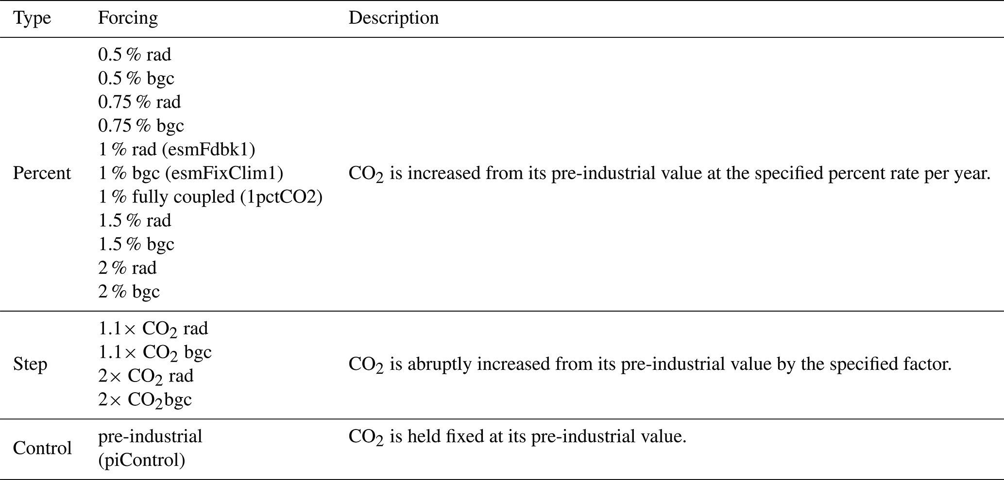
A1 Procedure to analyse the recovery of the generalized sensitivities

To perform the analysis described in the three steps above we employ a simple procedure introduced in Torres Mendonça et al. (2021b). The idea behind the procedure can be understood as follows. First, using the RFI method (Torres Mendonça et al., 2021a), we recover the generalized sensitivity taking pre-transformed data from increasingly longer time periods of the 1 % experiment. For each time period, we employ the recovered generalized sensitivity to predict the response of additional 0.5 % and 0.75 % experiments covering that same time period (for a description of the experiments see Table A1). Then, we measure the quality of the recovery of the generalized sensitivity by the quality of the prediction of the responses for these additional simulations. The quality of the prediction is quantified by the (dimensionless) prediction error:

$$\begin{array}{}\text{(A1)}& {\mathit{\epsilon }}_k:={\displaystyle \frac{\left|\right|\mathbf{\Delta }{\mathit{Y}}^k-\mathit{\chi }\star \mathbf{\Delta }{\mathit{f}}^k\left|\right|}{\left|\right|\mathbf{\Delta }{\mathit{Y}}^k\left|\right|}},\end{array}$$

where χ⋆Δf^k gives the predicted values, ⋆ stands in short for the convolution operation, ΔY^k and Δf^k are the response and the perturbation in experiment “k”, and χ is the response function recovered from the 1 % experiment. Because in the 1 % experiment the perturbation strength increases with time, also the signal-to-noise ratio of the data increases. On the other hand, higher perturbation strengths increase non-linearities. This results in the following trade-off: while a higher signal-to-noise ratio results in a recovery with better quality, larger non-linearities deteriorate the quality of the recovery. From this trade-off, by analysing the prediction error (A1) for different perturbation strengths of the 1 % experiment and also for different data pre-transformation techniques, one can (1) select the best pre-transformation technique for the recovery of the response function, (2) determine the maximum forcing strength for which the response function can be optimally recovered, and (3) estimate the linear regime of the response. For a more detailed description of this procedure please refer to Torres Mendonça et al. (2021b).

A2 Generalized sensitivity ${\mathit{\chi }}_{\mathit{\beta }}^{\left(\text{O}\right)}$

Pre-transformation techniques to recover ${\mathit{\chi }}_{\mathit{\beta }}^{\left(\text{O}\right)}$

Similarly to Torres Mendonça et al. (2021b), we recover ${\mathit{\chi }}_{\mathit{\beta }}^{\left(\text{O}\right)}\left(t\right)$ employing the RFI method in combination with two techniques. The first technique consists of simply taking Δc(t) as perturbation and deriving ${\mathit{\chi }}_{\mathit{\beta }}^{\left(\text{O}\right)}\left(t\right)$ from

$$\begin{array}{}\text{(A2)}& \mathrm{\Delta }{C}_{\mathrm{O}}^{\text{bgc}}\left(t\right)=\underset{\mathrm{0}}{\overset{t}{\int }}{\mathit{\chi }}_{\mathit{\beta }}^{\left(\text{O}\right)}(t-s)\mathrm{\Delta }c\left(s\right)\mathrm{d}s,\end{array}$$

where $\mathrm{\Delta }{C}_{\mathrm{O}}^{\mathrm{bgc}}\left(t\right)$ is the ocean carbon response in the bgc setup (see Table A1). Because we directly take Δc(t) for the recovery, we call this the no-transform technique.

Since Eq. (A2) is the equation employed in the generalized framework to describe the ocean biogeochemical response (compare Eq. 3), from this no-transform technique we will also obtain an estimate of the range of CO₂ perturbation strengths for which this response can be considered linear. This estimate is needed to address the question of what the linear regime is for which the generalized α–β–γ framework is valid in the MPI-ESM.

In the second technique, we consider the logarithm of c as perturbation and derive ${\mathit{\chi }}_{\mathit{\beta }}^{\left(\text{O}\right)}\left(t\right)$ from

$$\begin{array}{}\text{(A3)}& \mathrm{\Delta }{C}_{\text{O}}^{\text{bgc}}\left(t\right)=\underset{\mathrm{0}}{\overset{t}{\int }}{\mathit{\chi }}_{\mathit{\beta },\ln }^{\left(\text{O}\right)}(t-s)c_{\text{PI}}\ln {\displaystyle \frac{c\left(s\right)}{c_{\text{PI}}}}\mathrm{d}s,\end{array}$$

where c_PI is the pre-industrial value for atmospheric CO₂. Because we take instead of c its logarithm, we call this the log-transform technique.

This log-transform technique is inspired by the fact that non-linearities in the ocean carbon uptake come mainly from the dissolution of CO₂ in ocean surface water (see e.g. Joos and Bruno, 1996). Because with accumulation of CO₂ in upper layers of the ocean the ability for further uptake of CO₂ decreases (Hooß et al., 2001), we use a logarithmic representation for the perturbation to try to explicitly describe the non-linearity between CO₂ concentration and the carbon flux into the ocean. As explained in Torres Mendonça et al. (2021b, Eqs. (16), (18), and (19) in Sect. 4.1), employing Eq. (A3) has the advantage that ${\mathit{\chi }}_{\mathit{\beta },\ln }^{\left(\text{O}\right)}\left(t\right)={\mathit{\chi }}_{\mathit{\beta }}^{\left(\text{O}\right)}\left(t\right)$; i.e. by deriving ${\mathit{\chi }}_{\mathit{\beta },\ln }^{\left(\text{O}\right)}\left(t\right)$ from Eq. (A3) one obtains also the desired ${\mathit{\chi }}_{\mathit{\beta }}^{\left(\text{O}\right)}\left(t\right)$.

For both techniques ${\mathit{\chi }}_{\mathit{\beta }}^{\left(\text{O}\right)}\left(t\right)$ is derived enforcing monotonicity by the RFI algorithm (see Fig. 1 in Torres Mendonça et al., 2021a).

Recovery of ${\mathit{\chi }}_{\mathit{\beta }}^{\left(\text{O}\right)}$ and linear regime of the biogeochemical response of ocean carbon

Using the pre-transformation techniques described above, in the following we recover the generalized sensitivity ${\mathit{\chi }}_{\mathit{\beta }}^{\left(\text{O}\right)}$ and evaluate the quality of the results.

We start by deriving ${\mathit{\chi }}_{\mathit{\beta }}^{\left(\text{O}\right)}\left(t\right)$ from Eq. (A2) (no-transform technique) taking data from the 1 % bgc experiment. Following the procedure described in Sect. A1, we employ Eq. (A2) to predict the response from the 0.5 % and 0.75 % bgc experiments (see Table A1). Figure A1a shows the resulting prediction error (see Eq. A1) for the increasing time period of the data used to obtain ${\mathit{\chi }}_{\mathit{\beta }}^{\left(\text{O}\right)}\left(t\right)$ – note that on the x axis the CO₂ forcing strength in the 1 % bgc experiment at the end of the period is used. Similarly to the biogeochemical response of land carbon in Torres Mendonça et al. (2021b), minima are found for final forcing strengths below 100 ppm (about 94 ppm for the 0.75 % and 58 ppm for the 0.5 % bgc experiments), indicating the presence of strong non-linearities for forcing strengths above this value. Because both minima are “flat”, i.e. the error does not change substantially for values around the minima, we take as an estimate of the linear regime forcing the strengths below the highest minimum – about 94 ppm in the 0.75 % curve.

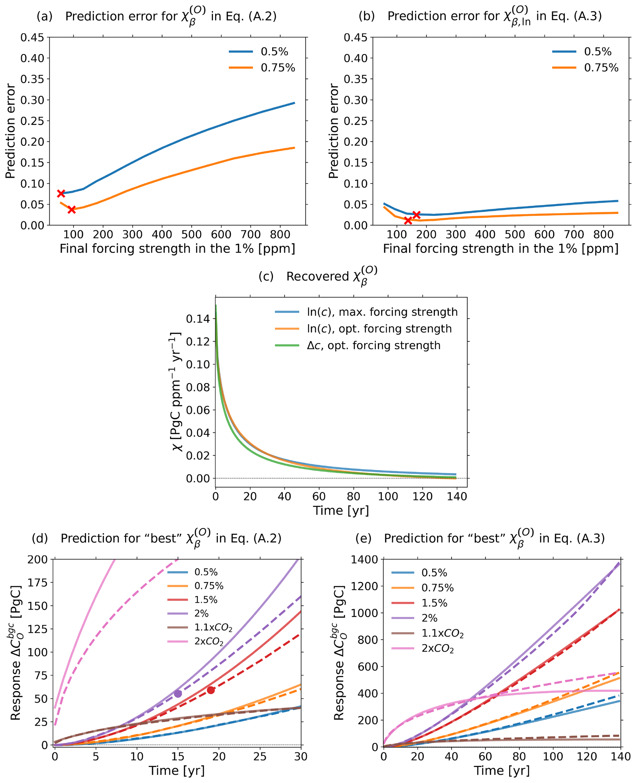
Figure A1 Generalized sensitivity ${\mathit{\chi }}_{\mathit{\beta }}^{\left(\text{O}\right)}\left(t\right)$ and prediction of responses from additional experiments. (a) Prediction error A1 for ${\mathit{\chi }}_{\mathit{\beta }}^{\left(\text{O}\right)}\left(t\right)$ derived with the no-transform technique employing Eq. (A2) for prediction. (b) Prediction error (A1) for ${\mathit{\chi }}_{\mathit{\beta }}^{\left(\text{O}\right)}\left(t\right)$ derived with the log-transform employing Eq. A3 for prediction. (c) Response function ${\mathit{\chi }}_{\mathit{\beta }}^{\left(\text{O}\right)}\left(t\right)$ recovered with the no-transform technique at optimal forcing strength (Δc), log-transform at optimal forcing strength (ln (c), opt. forcing strength), and log-transform at maximal forcing strength (ln (c), max forcing strength). (d) Prediction of additional experiments taking the “best” recovery of ${\mathit{\chi }}_{\mathit{\beta }}^{\left(\text{O}\right)}\left(t\right)$ (using the log-transform at optimal forcing strength) employed in Eq. (A2). (e) Prediction of additional experiments taking the “best” recovery of ${\mathit{\chi }}_{\mathit{\beta }}^{\left(\text{O}\right)}\left(t\right)$ (using the log-transform at optimal forcing strength) employed in Eq. (A3). Continuous lines are predictions and dashed lines are simulated responses from the MPI-ESM. Dots indicate the maximum value for which responses are predictable by Eq. (A2) according to the estimate of the linear regime (see text). For better visibility of the regions within the linear regime in (c), the responses are shown only for the first 30 years.

To try to improve the quality of the recovery, ${\mathit{\chi }}_{\mathit{\beta }}^{\left(\text{O}\right)}\left(t\right)$ was derived as well using the log-transform technique (Eq. A3). To see whether the quality of the recovery indeed improves, one must check if Eq. (A3) indeed accounts for some of the non-linearities in the response. If this is the case, then Eq. (A3) should predict the 0.5 % and 0.75 % bgc responses better than Eq. (A2). To check this, we recovered ${\mathit{\chi }}_{\mathit{\beta }}^{\left(\text{O}\right)}\left(t\right)$ by this log-transform technique and then employed the recovered ${\mathit{\chi }}_{\mathit{\beta }}^{\left(\text{O}\right)}\left(t\right)$ in Eq. (A3) to predict these responses. The resulting prediction error is shown in Fig. A1b. Overall the error is substantially smaller than in Fig. A1a. Minima are still found but now at values between 100 and 200 ppm and with smaller optimal errors. In contrast to Fig. A1a, after the minima the error increases only slightly for increasing final forcing strength. Therefore, Eq. (A3) seems to indeed account for some of the non-linearities in the response. Hence, with this approach one can derive ${\mathit{\chi }}_{\mathit{\beta }}^{\left(\text{O}\right)}\left(t\right)$ taking data from the 1 % bgc experiment until larger perturbation strengths and therefore higher signal-to-noise ratios than with the no-transform technique, making it in principle possible to recover ${\mathit{\chi }}_{\mathit{\beta }}^{\left(\text{O}\right)}\left(t\right)$ with better quality.

But despite the overall reduction in the prediction error, Fig. A1b still shows a slightly increasing trend in the prediction error after the minima, indicating the presence of possibly non-negligible non-linearities in the response. Therefore we check whether the log-transform technique indeed gives a better recovery for ${\mathit{\chi }}_{\mathit{\beta }}^{\left(\text{O}\right)}\left(t\right)$ by comparing the recovery from this technique with that from the no-transform technique. Figure A1c shows the response function recovered with each technique taking data from the 1 % bgc experiment until the optimal final forcing strength (we take 94 ppm or 30 years of the 1 % bgc experiment for the no-transform technique and 138 ppm or 50 years of the 1 % bgc experiment for the log-transform technique; the values correspond to the minima found in the 0.75 % curve, respectively, in Figs. A1a and b) and the response function recovered with the log-transform technique but taking data until the maximal final forcing strength in the 1 % bgc experiment, i.e. the whole time series (since for those forcing strengths the error in Fig. A1b is still small). As seen, all recovered response functions are very similar. This similarity is most likely due to the combination of an overall high signal-to-noise ratio of the ocean biogeochemical response (as indicated by the small errors even at small perturbation strengths in panels a and b) and only small contributions from non-linearities when employing the log-transform technique. This suggests that for the MPI-ESM ${\mathit{\chi }}_{\mathit{\beta }}^{\left(\text{O}\right)}\left(t\right)$ can be equally well recovered by either of the two techniques. Despite this result, we selected the log-transform technique for deriving ${\mathit{\chi }}_{\mathit{\beta }}^{\left(\text{O}\right)}\left(t\right)$ in Sects. 3 and 4 because this technique accounts for non-linearities that may cause a more significant error in the recovery for other models. But because panel (b) indicates that non-negligible non-linearities may still remain in the response even when employing this log-transform (because of the slightly increasing trend), we choose conservatively to take data only until the optimal forcing strength (138 ppm or 50 years of the 1 % bgc experiment) and not the full time series. As suggested by the small differences between the recoveries for the optimal and maximal forcing strengths in panel (c), taking data only until this optimal forcing strength does not significantly hinder the recovery of timescales on the order of the length of the full time series.

To obtain evidence that the recovered ${\mathit{\chi }}_{\mathit{\beta }}^{\left(\text{O}\right)}\left(t\right)$ indeed characterizes the biogeochemical response of the ocean carbon of the MPI-ESM to any temporal development of sufficiently weak atmospheric CO₂ perturbations, we show how well it predicts the model response for additional CO₂ perturbation experiments (see Table A1). The prediction is performed by convoluting the recovery of ${\mathit{\chi }}_{\mathit{\beta }}^{\left(\text{O}\right)}\left(t\right)$ selected above with the different CO₂ perturbation scenarios first via Eq. (A2), which is the equation employed in the generalized framework (compare with Eq. 3 in Sect. 2), and then via Eq. (A3) to see if by this equation the prediction is indeed further improved for all experiments. The result for the first case is shown in Fig. A1d. To better visualize the linear regime region where the approximation works, we show only the first 30 years. The responses for the 1.5 % and 2 % bgc experiments are marked with dots where the forcing strength exceeds 94 ppm, the maximal forcing strength corresponding to the linear regime estimated from Fig. A1a. As seen, the recovered ${\mathit{\chi }}_{\mathit{\beta }}^{\left(\text{O}\right)}\left(t\right)$ predicts almost perfectly the response from experiments whose forcing strengths are within the linear regime estimate, i.e. the 0.5 %, 0.75 %, and 1.1× CO₂ bgc experiments. It also predicts with reasonable quality of agreement the response from the 1.5 % and 2 % bgc experiments for forcing strengths within the estimated linear regime. As forcing strengths exceed the linear regime, the prediction starts to deviate from the model response. Likewise, the prediction fails for the whole 2× CO₂ bgc response because its forcing strength is larger than the linear regime estimate throughout the whole experiment. These results therefore suggest that ${\mathit{\chi }}_{\mathit{\beta }}^{\left(\text{O}\right)}\left(t\right)$ indeed characterizes the biogeochemical response of ocean carbon for any temporal development of atmospheric CO₂, as long as its strength is within the linear regime.

Figure A1e shows the prediction employing Eq. (A3). As seen, now the predictive power of ${\mathit{\chi }}_{\mathit{\beta }}^{\left(\text{O}\right)}\left(t\right)$ improves considerably, extending to the whole time series for all experiments. Some discrepancies are nevertheless encountered, especially for the last years of the 2× CO₂ bgc response. Such discrepancies are probably related to the relatively limited amount of information that data from 1 % experiments provide to recover response functions, as observed for the land carbon in Torres Mendonça et al. (2021b).

Despite these discrepancies, overall Fig. A1d and e show that the recovered ${\mathit{\chi }}_{\mathit{\beta }}^{\left(\text{O}\right)}\left(t\right)$ predicts the response from different experiments with reasonable quality up to certain perturbation strengths. Equation (A3) – employed for the prediction in Fig. A1e – demonstrates successful prediction of the response of the model up to higher perturbation strengths than Eq. (A2). Therefore, Eq. (A3) is probably more appropriate when the aim is to predict the separate biogeochemical response of the model to prescribed atmospheric CO₂ perturbations. On the other hand, Eq. (A2) is the equation employed in the generalized α–β–γ framework (first term on the right-hand side of Eq. 3). Therefore, when estimating the linear regime for the application of the generalized α–β–γ framework one has to consider for the ocean biogeochemical response the estimate obtained from Eq. (A2), i.e. the linear regime estimate indicated in panel (a).

The conclusions from this subsection therefore suggest that the best pre-transformation technique to derive ${\mathit{\chi }}_{\mathit{\beta }}^{\left(\text{O}\right)}\left(t\right)$ is the log-transform technique (Eq. A3), taking data until 138 ppm or 50 years of the 1 % bgc experiment, which corresponds to the first minimum for the prediction error in Fig. A1b. In addition, the linear regime for the ocean biogeochemical response in the generalized α–β–γ framework (first term on the right-hand side of Eq. 3) is about 94 ppm, as estimated from Fig. A1a.

A3 Generalized sensitivity ${\mathit{\chi }}_{\mathit{\gamma }}^{\left(\text{O}\right)}$

Technique to recover ${\mathit{\chi }}_{\mathit{\gamma }}^{\left(\text{O}\right)}$

In this subsection we recover ${\mathit{\chi }}_{\mathit{\gamma }}^{\left(\text{O}\right)}\left(t\right)$. Since, as will be seen, no strong non-linearities are present in the response, ${\mathit{\chi }}_{\mathit{\gamma }}^{\left(\text{O}\right)}\left(t\right)$ is well recovered without any pre-transformations from

$$\begin{array}{}\text{(A4)}& \mathrm{\Delta }{C}_{\text{O}}^{\text{rad}}\left(t\right)=\underset{\mathrm{0}}{\overset{t}{\int }}{\mathit{\chi }}_{\mathit{\gamma }}^{\left(\text{O}\right)}(t-s)\mathrm{\Delta }{T}_{\text{O}}\left(s\right)\mathrm{d}s,\end{array}$$

where $\mathrm{\Delta }{C}_{\text{O}}^{\text{rad}}\left(t\right)$ is the ocean carbon response in the rad setup. Because the quality of the recovery depends on the quality of the estimate of the noise in the data, and this estimate may be improved by enforcing monotonicity (see Torres Mendonça et al., 2021a), we assume that ${\mathit{\chi }}_{\mathit{\gamma }}^{\left(\text{O}\right)}$ is monotonic and recover it enforcing monotonicity by the RFI method. An indication of the quality of the recovery will be obtained below by checking how well the recovered ${\mathit{\chi }}_{\mathit{\gamma }}^{\left(\text{O}\right)}$ predicts the model response in different perturbation experiments.

Recovery of ${\mathit{\chi }}_{\mathit{\gamma }}^{\left(\text{O}\right)}$ and linear regime of the radiative response of ocean carbon

We start by recovering ${\mathit{\chi }}_{\mathit{\gamma }}^{\left(\text{O}\right)}\left(t\right)$ from the 1 % rad experiment. To evaluate the quality of the recovery, following the procedure from Sect. A1 we employed the recovered ${\mathit{\chi }}_{\mathit{\gamma }}^{\left(\text{O}\right)}\left(t\right)$ in Eq. (A4) to predict the 0.5 % and 0.75 % rad responses. The prediction error is plotted in Fig. A2a as a function of the final forcing strength in the 1 % rad experiment. As seen, the error decreases with increasing final forcing strength, indicating that no strong non-linearities are present in the response. As a result, the response can be considered linear for the whole range of forcing strengths in the 1 % rad experiment (temperatures up to around 4 K). Hence we choose to recover ${\mathit{\chi }}_{\mathit{\gamma }}^{\left(\text{O}\right)}\left(t\right)$ for the investigation in the main text by taking data from the full 1 % rad experiment.

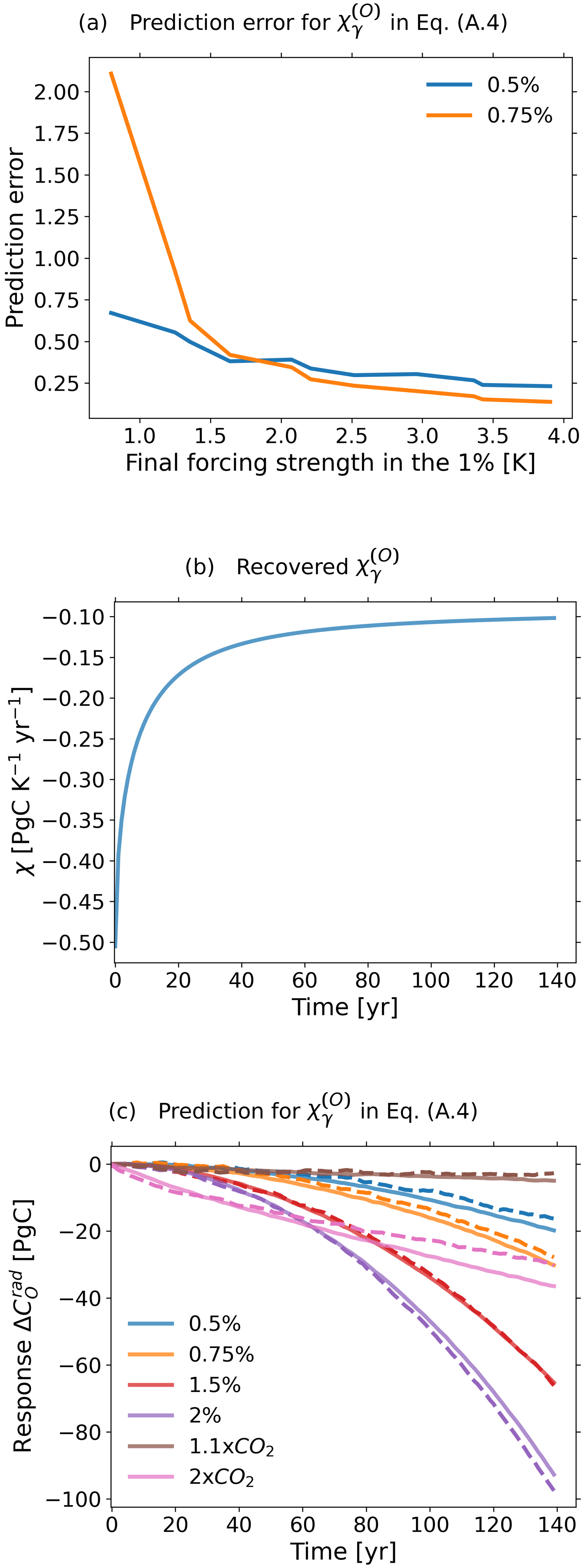
Figure A2 Generalized sensitivity ${\mathit{\chi }}_{\mathit{\gamma }}^{\left(\text{O}\right)}\left(t\right)$ and prediction of responses from additional experiments. (a) Prediction error (A1) employing the recovered ${\mathit{\chi }}_{\mathit{\gamma }}^{\left(\text{O}\right)}\left(t\right)$ in Eq. (A4). (b) Recovered response function ${\mathit{\chi }}_{\mathit{\gamma }}^{\left(\text{O}\right)}\left(t\right)$. (c) Prediction of additional experiments employing the recovered ${\mathit{\chi }}_{\mathit{\gamma }}^{\left(\text{O}\right)}\left(t\right)$ in Eq. (A4). Continuous lines are predictions and dashed lines are simulated responses from the MPI-ESM. For more details see text.

The resulting ${\mathit{\chi }}_{\mathit{\gamma }}^{\left(\text{O}\right)}\left(t\right)$ recovered in this way is shown in Fig. A2b. The negativity of ${\mathit{\chi }}_{\mathit{\gamma }}^{\left(\text{O}\right)}\left(t\right)$ reflects the fact that as temperatures rise, globally the ocean loses carbon to the atmosphere. This is consistent with the results shown in Fig. A2c, which shows the model responses from the different rad experiments and the prediction from the recovered ${\mathit{\chi }}_{\mathit{\gamma }}^{\left(\text{O}\right)}\left(t\right)$. Because in these experiments only the radiative effect of CO₂ is active (while the biogeochemical effect is switched off), temperatures rise, leading to the mentioned global loss of ocean carbon to the atmosphere reflected by the negative responses. The quality of agreement between the model responses and the predictions from ${\mathit{\chi }}_{\mathit{\gamma }}^{\left(\text{O}\right)}\left(t\right)$ suggests that indeed the recovered ${\mathit{\chi }}_{\mathit{\gamma }}^{\left(\text{O}\right)}\left(t\right)$ characterizes the radiative response of ocean carbon not only for the few perturbation experiments considered here but to any temporal development of weak CO₂ perturbations and is therefore a true property of the MPI-ESM itself.

In summary, since the response can be considered linear over the whole 1 % rad experiment, we chose to derive ${\mathit{\chi }}_{\mathit{\gamma }}^{\left(\text{O}\right)}\left(t\right)$ in Sects. 3 and 4 from Eq. (A4) taking data from the full experiment.

A4 Generalized sensitivities ${\mathit{\chi }}_{\mathit{\alpha }}^{\left(\text{L}\right)}$ and ${\mathit{\chi }}_{\mathit{\alpha }}^{\left(\text{O}\right)}$

Pre-transformation techniques to recover ${\mathit{\chi }}_{\mathit{\alpha }}^{\left(\text{L}\right)}$ and ${\mathit{\chi }}_{\mathit{\alpha }}^{\left(\text{O}\right)}$

Following Sect. A2 we recover ${\mathit{\chi }}_{\mathit{\alpha }}^{\left(\text{L}\right)}\left(t\right)$ and ${\mathit{\chi }}_{\mathit{\alpha }}^{\left(\text{O}\right)}\left(t\right)$ by employing two different techniques. In the first technique we recover the sensitivities from Eqs. (4) and (5), i.e. without any pre-transformation. From this first technique we will also obtain an estimate of the linear regime for the temperature responses as described in the generalized α–β–γ framework.

Because CO₂ radiative forcing is known to increase logarithmically with atmospheric CO₂ concentration (Myhre et al., 1998), we also derive ${\mathit{\chi }}_{\mathit{\alpha }}^{\left(\text{L}\right)}\left(t\right)$ and ${\mathit{\chi }}_{\mathit{\alpha }}^{\left(\text{O}\right)}\left(t\right)$ using a logarithmic pre-transformation:

$$\begin{array}{}\text{(A5)}& {\displaystyle }\mathrm{\Delta }{T}_{\text{L}}\left(t\right)=\underset{\mathrm{0}}{\overset{t}{\int }}{\mathit{\chi }}_{\mathit{\alpha },\ln }^{\left(\text{L}\right)}(t-s)c_{\text{PI}}\ln {\displaystyle \frac{c\left(s\right)}{c_{\text{PI}}}}\mathrm{d}s,\text{(A6)}& {\displaystyle }\mathrm{\Delta }{T}_{\text{O}}\left(t\right)=\underset{\mathrm{0}}{\overset{t}{\int }}{\mathit{\chi }}_{\mathit{\alpha },\ln }^{\left(\text{O}\right)}(t-s)c_{\text{PI}}\ln {\displaystyle \frac{c\left(s\right)}{c_{\text{PI}}}}\mathrm{d}s.\end{array}$$

As explained in Torres Mendonça et al. (2021b, Sect. 4), the resulting ${\mathit{\chi }}_{\mathit{\alpha },\ln }^{\left(\text{L}\right)}\left(t\right)={\mathit{\chi }}_{\mathit{\alpha }}^{\left(\text{L}\right)}\left(t\right)$ and ${\mathit{\chi }}_{\mathit{\alpha },\ln }^{\left(\text{O}\right)}\left(t\right)={\mathit{\chi }}_{\mathit{\alpha }}^{\left(\text{O}\right)}\left(t\right)$.

Recovery of ${\mathit{\chi }}_{\mathit{\alpha }}^{\left(\text{L}\right)}$, ${\mathit{\chi }}_{\mathit{\alpha }}^{\left(\text{O}\right)}$, and linear regime of temperature responses

We start by recovering ${\mathit{\chi }}_{\mathit{\alpha }}^{\left(\text{L}\right)}\left(t\right)$ and ${\mathit{\chi }}_{\mathit{\alpha }}^{\left(\text{O}\right)}\left(t\right)$ without any pre-transformation (Eqs. 4 and 5) taking data from the 1 % rad experiment. As in the previous subsections, to evaluate the quality of the recoveries we employed them once more in Eqs. (4) and (5) to predict the responses from the 0.5 % and 0.75 % rad experiments. The prediction error is plotted in Figs. A3a and A4a. As seen, in both figures the error decreases until about 279 ppm, presenting after that in Fig. A3a a clear increase and in Fig. A4a a slight decrease followed by an increase for the 0.5 % rad response and an approximately constant behaviour for the 0.75 % rad response. Therefore we conservatively estimate the linear regime as perturbation strengths below 279 ppm for both land and ocean temperature responses.

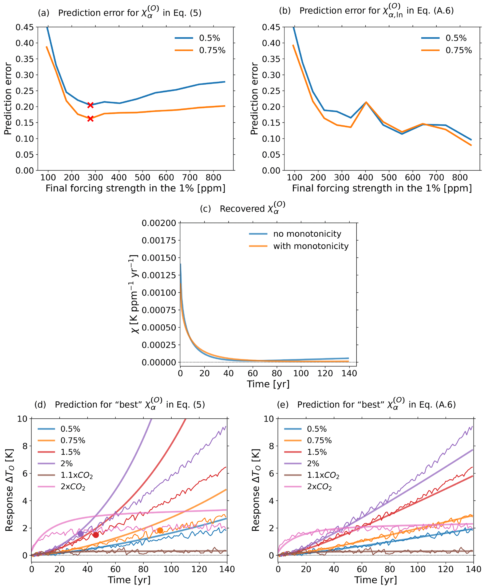
Figure A3 Generalized sensitivity ${\mathit{\chi }}_{\mathit{\alpha }}^{\left(\text{O}\right)}\left(t\right)$ and prediction of responses from additional experiments. (a) Prediction error A1 for ${\mathit{\chi }}_{\mathit{\alpha }}^{\left(\text{O}\right)}\left(t\right)$ derived with the no-transform technique employing Eq. (5) for prediction. (b) Prediction error (A1) for ${\mathit{\chi }}_{\mathit{\alpha }}^{\left(\text{O}\right)}\left(t\right)$ derived with the log-transform employing Eq. (A6) for prediction. (c) Response function ${\mathit{\chi }}_{\mathit{\alpha }}^{\left(\text{O}\right)}\left(t\right)$ recovered with the log-transform both enforcing and not enforcing monotonicity. (d) Prediction of additional experiments taking the “best” recovery of ${\mathit{\chi }}_{\mathit{\alpha }}^{\left(\text{O}\right)}\left(t\right)$ (using the log-transform enforcing monotonicity) employed in Eq. (5). (e) Prediction of additional experiments taking the “best” recovery of ${\mathit{\chi }}_{\mathit{\alpha }}^{\left(\text{O}\right)}\left(t\right)$ (using the log-transform enforcing monotonicity) employed in Eq. (A6). Thick lines are predictions and thin lines are responses from the MPI-ESM. Dots indicate the maximum value for which responses are predictable by Eq. (5) according to the estimate of the linear regime. For more details see text.

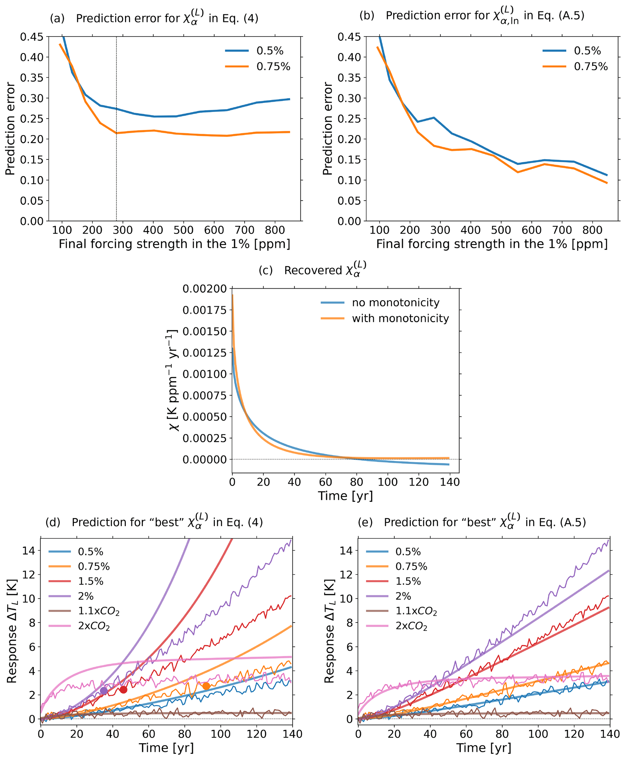
Figure A4 Generalized sensitivity ${\mathit{\chi }}_{\mathit{\alpha }}^{\left(\text{L}\right)}\left(t\right)$ and prediction of responses from additional experiments. (a) Prediction error (A1) for ${\mathit{\chi }}_{\mathit{\alpha }}^{\left(\text{L}\right)}\left(t\right)$ derived with the no-transform technique employing Eq. (4) for prediction. (b) Prediction error (A1) for ${\mathit{\chi }}_{\mathit{\alpha }}^{\left(\text{L}\right)}\left(t\right)$ derived with the log-transform employing Eq. (A5) for prediction. (c) Response function ${\mathit{\chi }}_{\mathit{\alpha }}^{\left(\text{L}\right)}\left(t\right)$ recovered with the log-transform both enforcing and not enforcing monotonicity. (d) Prediction of additional experiments taking the “best” recovery of ${\mathit{\chi }}_{\mathit{\alpha }}^{\left(\text{L}\right)}\left(t\right)$ (using the log-transform enforcing monotonicity) employed in Eq. (4). (e) Prediction of additional experiments taking the “best” recovery of ${\mathit{\chi }}_{\mathit{\alpha }}^{\left(\text{L}\right)}\left(t\right)$ (using the log-transform enforcing monotonicity) employed in Eq. (A5). Thick lines are predictions and thin lines are responses from the MPI-ESM. Dots indicate the maximum value for which responses are predictable by Eq. (4) according to the estimate of the linear regime. For more details see text.

To assess whether the log-transform technique (Eqs. A5 and A6) indeed improves the recovery of ${\mathit{\chi }}_{\mathit{\alpha }}^{\left(\text{L}\right)}\left(t\right)$ and ${\mathit{\chi }}_{\mathit{\alpha }}^{\left(\text{O}\right)}\left(t\right)$, analogously to Sect. A2 we check whether Eqs. (A5) and (A6) indeed account for non-linearities in the response. If this is the case, then Eqs. (A5) and (A6) should predict the 0.5 % and 0.75 % rad responses better than Eqs. (4) and (5). To evaluate this, we recovered ${\mathit{\chi }}_{\mathit{\alpha }}^{\left(\text{L}\right)}\left(t\right)$ and ${\mathit{\chi }}_{\mathit{\alpha }}^{\left(\text{O}\right)}\left(t\right)$ from Eqs. (A5) and (A6) taking data once more from the 1 % rad experiment and then employed the recovered response functions in Eqs. (A5) and (A6) to predict the 0.5 % and 0.75 % rad responses. The resulting prediction error is shown in Figs. A3b and A4b. As seen in both figures, now the prediction error clearly decreases for increasing final forcing strength, indicating that no strong non-linearities are present in the response. This clear decreasing trend in the prediction error indicates that the log-transform technique (Eqs. A5 and A6) is indeed more appropriate to recover ${\mathit{\chi }}_{\mathit{\alpha }}^{\left(\text{L}\right)}\left(t\right)$ and ${\mathit{\chi }}_{\mathit{\alpha }}^{\left(\text{O}\right)}\left(t\right)$.

Therefore in Figs. A3c and A4c we show the response functions recovered with the log-transform technique. Plotted are recoveries by the RFI method both enforcing and not enforcing monotonicity. As seen, the recoveries obtained without enforcing monotonicity are approximately monotonic, so differences between the two types of recovery are small. Hence in the next sections we choose to derive ${\mathit{\chi }}_{\mathit{\alpha }}^{\left(\text{L}\right)}\left(t\right)$ and ${\mathit{\chi }}_{\mathit{\alpha }}^{\left(\text{O}\right)}\left(t\right)$ employing the log-transform and enforcing monotonicity by the RFI method. As already mentioned above (see also Torres Mendonça et al., 2021a), the advantage of enforcing monotonicity is that one may improve the noise level estimate used in the RFI method and thereby improve the quality of the recovery.

To obtain evidence that the recovered ${\mathit{\chi }}_{\mathit{\alpha }}^{\left(\text{L}\right)}\left(t\right)$ and ${\mathit{\chi }}_{\mathit{\alpha }}^{\left(\text{O}\right)}\left(t\right)$ indeed characterize the land and ocean temperature responses to any temporal development of weak CO₂ perturbations, we show how well they predict additional experiments. Following Sect. A2 we first show the predictive power of ${\mathit{\chi }}_{\mathit{\alpha }}^{\left(\text{L}\right)}\left(t\right)$ and ${\mathit{\chi }}_{\mathit{\alpha }}^{\left(\text{O}\right)}\left(t\right)$ when employed in Eqs. (4) and (5), i.e. without pre-transformations. In Figs. A3d and A4d we plot the predictions by Eqs. (4) and (5) taking the recoveries selected above (log-transform technique enforcing monotonicity). The responses for the 0.75 %, 1.5 %, and 2 % rad experiments are marked with dots where the forcing strength exceeds 279 ppm – the maximal forcing strength corresponding to the linear regime estimated from Figs. A3a and A4a. As seen, the recovered response functions predict the model responses with some overestimation but still with reasonable quality of agreement⁵ for forcing strengths within the estimated linear regime, i.e. for the entire 1.1× CO₂ and 0.5 % rad experiments and for the 0.75 %, 1.5 %, and 2 % rad experiments for values preceding the dots. For these three latter experiments predictions start to strongly deviate from the responses as forcing strengths exceed the estimated linear regime. Likewise, the predictions fail basically for the whole 2× CO₂ rad response because its forcing strength is larger than the linear regime estimate throughout the whole experiment.

As expected from the known logarithmic relationship between radiative forcing and CO₂ concentration, the predictive power of ${\mathit{\chi }}_{\mathit{\alpha }}^{\left(\text{L}\right)}\left(t\right)$ and ${\mathit{\chi }}_{\mathit{\alpha }}^{\left(\text{O}\right)}\left(t\right)$ improves when employing Eqs. (A5) and (A6) instead of Eqs. (4) and (5) (see Figs. A3e and A4e). Almost all responses are well predicted for the whole time series. The exceptions are the last years of the 1.5 % and 2 % rad responses, which indicates a deviation from linearity for those levels of perturbation strength.

Torres Mendonça et al. (2021b)Torres Mendonça et al. (2021b)

Table A2 Techniques identified to derive the generalized sensitivities in Sects. 3 and 4 and the linear regime of the responses in the generalized framework according to the analyses from Torres Mendonça et al. (2021b) and Appendix A. The column “Pre-transformation technique” refers to the data pre-transformation that led to the best recovery of the generalized sensitivity. The column “Data length for best technique” refers to the length of the time series from the 1 % experiment after transformation by the referred technique that was taken to derive the generalized sensitivity with the best trade-off between signal-to-noise ratio and non-linearities. The column “Linear regime” refers to the range of forcing strengths for which the response characterized by a particular generalized sensitivity in the generalized framework can be considered linear (i.e. the linear regime for each term on the right-hand side of Eqs. 2–5). All generalized sensitivities were derived enforcing monotonicity by the RFI algorithm (Torres Mendonça et al., 2021a).

As in Sect. A2, overall the prediction results suggest that indeed the recovered response functions characterize the land and ocean temperature responses to any temporal development of atmospheric CO₂ up to certain perturbation strengths. While Eqs. (A5) and (A6) are more appropriate when the aim is simply to predict model responses because of their extended predictive power, Eqs. (4) and (5) are the equations actually employed in the generalized α–β–γ framework, so for the application of the framework one must consider the linear regime of the temperature responses estimated from Figs. A3a and A4a.

In summary, the conclusions from this subsection suggest that the best approach to derive ${\mathit{\chi }}_{\mathit{\alpha }}^{\left(\text{L}\right)}\left(t\right)$ and ${\mathit{\chi }}_{\mathit{\alpha }}^{\left(\text{O}\right)}\left(t\right)$ is the log-transform technique (Eqs. A5 and A6), taking data from the full 1 % rad experiment. The linear regime for the land and ocean temperature responses in the generalized α–β–γ framework (Eqs. 5 and 4) is about 279 ppm, as estimated from Figs. A3a and A4a.

A5 Selection of techniques to recover ${\mathit{\chi }}_{\mathit{\gamma }}^{\left(\text{L}\right)}\left(t\right)$ and ${\mathit{\chi }}_{\mathit{\beta }}^{\left(\text{L}\right)}\left(t\right)$

To recover ${\mathit{\chi }}_{\mathit{\gamma }}^{\left(\text{L}\right)}\left(t\right)$ and ${\mathit{\chi }}_{\mathit{\beta }}^{\left(\text{L}\right)}\left(t\right)$ we use the conclusions from Torres Mendonça et al. (2021b). Because the radiative response of land carbon can be considered linear for the whole range of perturbation strengths in the 1 % rad experiment (Torres Mendonça et al., 2021b, Sect. 3), ${\mathit{\chi }}_{\mathit{\gamma }}^{\left(\text{L}\right)}\left(t\right)$ is derived taking data without any pre-transformation from the full 1 % rad experiment by employing

$$\begin{array}{}\text{(A7)}& \mathrm{\Delta }{C}_{\text{L}}^{\text{rad}}\left(t\right)=\underset{\mathrm{0}}{\overset{t}{\int }}{\mathit{\chi }}_{\mathit{\gamma }}^{\left(\text{L}\right)}(t-s)\mathrm{\Delta }{T}_{\text{L}}\left(s\right)\mathrm{d}s,\end{array}$$

where $\mathrm{\Delta }{C}_{\text{L}}^{\text{rad}}\left(t\right)$ is the land carbon response in the rad setup. Because the obtained ${\mathit{\chi }}_{\mathit{\gamma }}^{\left(\text{L}\right)}\left(t\right)$ is monotonic (without enforcing monotonicity), we assume monotonicity when deriving ${\mathit{\chi }}_{\mathit{\gamma }}^{\left(\text{L}\right)}\left(t\right)$ for all other CMIP5 models so that all generalized sensitivities are derived enforcing monotonicity by the RFI method (as mentioned above and explained in Sect. 3.5 of Torres Mendonça et al., 2021a, this assumption may further improve the quality of the recovery).

To derive ${\mathit{\chi }}_{\mathit{\beta }}^{\left(\text{L}\right)}\left(t\right)$, conclusions from Sect. 4 of Torres Mendonça et al. (2021b) suggest that the best approach is the NPP-transform technique analysed there: first derive the response function χ_NPP(t) from

$$\begin{array}{}\text{(A8)}& \mathrm{\Delta }{C}_{\text{L}}^{\text{bgc}}\left(t\right)=\underset{\mathrm{0}}{\overset{t}{\int }}{\mathit{\chi }}_{\mathrm{NPP}}(t-s)\mathrm{\Delta }\mathrm{NPP}\left(s\right)\mathrm{d}s,\end{array}$$

and then transform the obtained χ_NPP(t) into the desired ${\mathit{\chi }}_{\mathit{\beta }}^{\left(\text{L}\right)}\left(t\right)$ via

$$\begin{array}{}\text{(A9)}& {\mathit{\chi }}_{\mathit{\beta }}^{\left(\text{L}\right)}\left(t\right)={\mathit{\chi }}_{\mathrm{NPP}}\left(t\right){\displaystyle \frac{\partial \mathrm{NPP}}{\partial c}}{|}_{c=c_{{}_{\text{PI}}}},\end{array}$$

where c_PI is the pre-industrial value for atmospheric CO₂. Because the prediction error plot for χ_NPP(t) presents minima (see Fig. 6c in Torres Mendonça et al., 2021b), following the reasoning from Sect. A2 we choose conservatively to take data only until the first minimum, which corresponds to 279 ppm or 70 years of the 1 % bgc experiment.

A6 Summary of best techniques for recovery of the generalized sensitivities

With the results presented in the preceding subsections we can now summarize the best techniques identified to recover the generalized sensitivities for our study. A general summary of the identified techniques is given in Table A2. The table indicates which is (1) the best pre-transformation technique to derive each generalized sensitivity, (2) the respective equation used for the derivation, (3) the optimal time series length taken for recovery using the best pre-transformation technique, and (4) the linear regime of the respective response in the generalized α–β–γ framework (i.e. the linear regime for each term on the right-hand side of Eqs. 2–5).

Because the linear regime for the biogeochemical response of land and ocean carbon is restricted to forcing strengths even smaller than that for temperature responses (4) and (5) – and obviously also smaller than that for the radiative responses of land and ocean carbon, which are linear for the whole 1 % rad experiment, as seen in Torres Mendonça et al. (2021b) and Sect. A3 – the applicability of the generalized α–β–γ framework as a whole is limited by the linear regime of the biogeochemical responses, which is estimated as forcing strengths up to about 94 ppm.

With this subsection we complete the recovery of all generalized sensitivities for the MPI-ESM. The approaches selected here are employed to recover the generalized sensitivities for all CMIP5 models in the main text.

Appendix B: Calculation of the timescale-dependent airborne fraction from emission-driven simulations

In this appendix we explain in detail how we derived the airborne fraction $\stackrel{\mathrm{̃}}{A}\left(p\right)$ from emission-driven simulations for the demonstration of Sect. 3. For the derivation we followed the three steps described in Sect. 3.1.

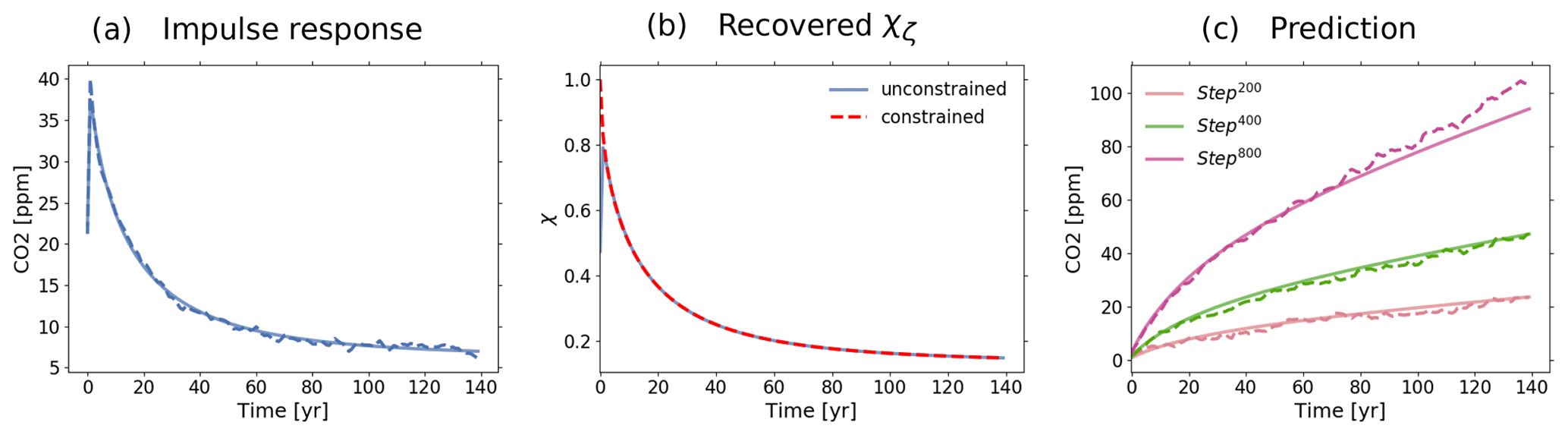
Figure B1 Response function χ_ζ(t) recovered from impulse-emission experiment Impulse¹⁰⁰. (a) Impulse response and fit by χ_ζ(t); (b) χ_ζ(t) recovered with and without enforcing the constraint χ_ζ(0)=1; (c) prediction of different experiments employing the recovered χ_ζ(t) in Eq. (16). For more details see text.

In the first step, we recovered χ_ζ(t) taking data from an impulse-emission experiment. In this experiment, starting from a standard pre-industrial control run (see “esmControl” in Taylor et al., 2012), we perturbed the system by a small impulse in emissions of 100 Pg C yr⁻¹ (as in Joos et al., 2013) during the first year. Therefore we name this experiment Impulse¹⁰⁰. The advantage of using data from this type of experiment is that the impulse response is from a practical point of view directly the desired linear response function χ_ζ(t), so errors from the ill-posedness of Eq. (16) (Torres Mendonça et al., 2021a) can be avoided. Nevertheless, the disadvantage is that the small impulse perturbation strength leads to a response with poor signal-to-noise ratio, which deteriorates the recovery of χ_ζ(t). Therefore, instead of taking data from only one realization of the experiment, we performed an ensemble of five realizations with initial conditions taken 100 years apart from one another (as in Lembo et al., 2020) and then took the data from the ensemble average of the response. This procedure is in agreement with linear response theory because strictly the linear response function characterizes only the ensemble average of the response (e.g. Torres Mendonça et al., 2021a). Taking the data from the ensemble average we employed the RFI method to recover χ_ζ(t). Although in principle a special method is not needed to recover χ_ζ(t) because the impulse response is directly the linear response function, by employing the RFI method we obtain not only χ_ζ(t) but also the spectrum of internal timescales of the response (Torres Mendonça et al., 2021a), from which the Laplace transform ${\stackrel{\mathrm{̃}}{\mathit{\chi }}}_{\mathit{\zeta }}\left(p\right)$ in Eq. (18) can be analytically calculated.

The resulting impulse response after taking the ensemble average and the fit by the recovered χ_ζ(t) are shown in Fig. B1a. One sees that the experiment is not a perfect impulse experiment because the impulse extends even beyond the first year. This may be related to internal interpolations in the model when computing the emissions within the time interval of 1 year. Such a problem leads to an error in the estimation of χ_ζ(0), which must be 1 by conservation of mass: for an impulse in emissions E(t)=aδ(t), it must be that at t=0 the impulse response $\mathrm{\Delta }{c}_{\mathit{\delta }}\left(\mathrm{0}\right)=a{\mathit{\chi }}_{\mathit{\zeta }}\left(\mathrm{0}\right)=a$ because land carbon and ocean carbon have no time to react; hence χ_ζ(0)=1. To avoid this error, we recalculated χ_ζ(t) using the same regularization parameter obtained from the RFI method but employing a Lagrange multiplier to account for this constraint (see Appendix C). The result for both recoveries is shown in Fig. B1b. The response functions are almost identical except for χ_ζ(0), which is corrected by enforcing the constraint χ_ζ(0)=1.

To make sure that the impulse response is within the linear regime and therefore that the recovery of χ_ζ(t) is not spoiled by non-linearities, in line with the procedure in Sect. A, we check the quality of the recovered χ_ζ(t) by employing it to predict additional emission-driven experiments via Eq. (16). For the additional experiments we chose step-emission experiments where starting from the control run the system is perturbed by abrupt, constant emissions of 1.43, 2.86, and 5.71 Pg C yr⁻¹, which by the end of the simulation result in cumulative emissions of 200, 400, and 800 Pg C. For this reason we name these experiments Step²⁰⁰, Step⁴⁰⁰, and Step⁸⁰⁰, respectively. The quality of the prediction is shown in Fig. B1c. As seen, the obtained χ_ζ(t) can predict almost all responses with reasonable accuracy for the whole time series. The only exception is over the last years of the Step⁸⁰⁰ experiment. The discrepancy encountered there is nevertheless in agreement with results from Torres Mendonça et al. (2021b) and from Appendix A that show that strong non-linear contributions to the biogeochemical response of land and ocean carbon start to arise at about 94 ppm. As a consequence, the identified discrepancy is not a result of non-linearities spoiling the recovery of χ_ζ(t) but rather a result of non-linearities that arise in the response of the Step⁸⁰⁰ experiment, which can therefore not be completely predicted by χ_ζ(t).

Hence, overall these results suggest that the recovery of χ_ζ(t) is not spoiled by non-linearities and is thus a good candidate to be used to compute the airborne fraction. Therefore χ_ζ(t) was Laplace-transformed and the airborne fraction was finally derived by applying Eq. (18).

Further evidence of the reliability of our numerics is obtained by examining the agreement of the resulting airborne fraction (Fig. 1) with theoretical expectations: $\stackrel{\mathrm{̃}}{A}\left(p\right)$ indeed converges to 1 for $\mathrm{1}/p\to \mathrm{0}$, as expected by Eq. (19), and $\mathrm{0}\le \stackrel{\mathrm{̃}}{A}\left(p\right)\le \mathrm{1}$ for all timescales $\mathrm{1}/p$, as expected by the considerations of Appendix D.

Appendix C: Calculation of χ_ζ(t) enforcing the constraint χ_ζ(0)=1

This appendix complements Appendix B to show how χ_ζ(t) is calculated by the RFI method enforcing in addition the theoretically exact relation χ_ζ(0)=1. The RFI method recovers a response function χ(t) employing the Tikhonov–Phillips regularization, with the regularization parameter λ determined from an estimate of the noise in the data (Torres Mendonça et al., 2021a). But the RFI method does not account for the desired constraint χ_ζ(0)=1. Therefore to derive χ_ζ(t) enforcing this constraint we proceed in two steps. First, we derive χ_ζ(t) by the RFI method without the constraint, obtaining thereby the value of λ. Then, we use the obtained λ to derive χ_ζ(t) employing the same regularization procedure from the RFI method but accounting in addition for the constraint χ_ζ(0)=1 by the method of Lagrange multipliers (Sundaram et al., 1996; Selesnick, 2013).

After obtaining λ by the RFI method in the first step, the derivation of χ_ζ(t) in the second step proceeds as follows. As in the RFI method, we assume χ_ζ(t) to be given by

$$\begin{array}{}\text{(C1)}& {\mathit{\chi }}_{\mathit{\zeta }}\left(t\right)=\underset{-\mathrm{\infty }}{\overset{\mathrm{\infty }}{\int }}q\left(\mathit{\tau }\right)e^{-t/\mathit{\tau }}\mathrm{d}{\log }_{\mathrm{10}}\mathit{\tau },\end{array}$$

where q(τ) is the spectrum of internal timescales. By plugging Eq. (C1) into Eq. (16) and prescribing a distribution of timescales τ, the problem of finding χ_ζ(t) boils down to finding the spectrum q(τ). Once q(τ) is derived, χ_ζ(t) follows from Eq. (C1). For more details please refer to Torres Mendonça et al. (2021a).

To understand how the constraint can be enforced, one has to consider

$$\begin{array}{}\text{(C2)}& {\mathit{\chi }}_{\mathit{\zeta }}\left(\mathrm{0}\right)=\underset{-\mathrm{\infty }}{\overset{\mathrm{\infty }}{\int }}q\left(\mathit{\tau }\right)\mathrm{d}{\log }_{\mathrm{10}}\mathit{\tau }.\end{array}$$

Equation (C2) can be discretized using the prescribed distribution of timescales equally spaced at a logarithmic scale between maximum and minimum values τ_max and τ_min (Torres Mendonça et al., 2021a). This discretization gives

$$\begin{array}{}\text{(C3)}& {\mathit{\chi }}_{\mathit{\zeta }}\left(\mathrm{0}\right)\approx \mathrm{\Delta }{\log }_{\mathrm{10}}\mathit{\tau }\sum _{j=\mathrm{0}}^{M-\mathrm{1}}{q}_j,\end{array}$$

where M is the number of q_j terms and $\mathrm{\Delta }{\log }_{\mathrm{10}}\mathit{\tau }:=({\log }_{\mathrm{10}}{\mathit{\tau }}_{\max }-{\log }_{\mathrm{10}}{\mathit{\tau }}_{\min })/M$ is the spacing between the timescales. Following Torres Mendonça et al. (2021a, Sect. 4.2), we take M=30, τ_min=0.1, and τ_max=10⁵. Using Eq. (C3) one can write the desired constraint χ_ζ(0)=1 in a discrete formulation as

$$\begin{array}{}\text{(C4)}& \mathbf{C}\mathit{q}=\mathrm{1},\end{array}$$

where C is the row matrix $\mathbf{C}:=[\mathrm{1},\mathrm{1},\mathrm{\dots },\mathrm{1}]\mathrm{\Delta }{\log }_{\mathrm{10}}\mathit{\tau }$.

Knowing how to discretely account for the desired constraint the spectrum q can now be derived. The procedure consists of minimizing the standard cost function employed in the Tikhonov–Phillips regularization (see e.g. Hansen, 2010, p. 60), which is also done in the RFI method but now subject to the constraint (C4); i.e.

$$\begin{array}{}\text{(C5)}& \underset{{\mathit{q}}_{\mathit{\lambda }}}{min}\left(\left|\right|\mathbf{\Delta }\mathit{Y}-\mathbf{A}{\mathit{q}}_{\mathit{\lambda }}|{|}^{\mathrm{2}}+\mathit{\lambda }|\left|{\mathit{q}}_{\mathit{\lambda }}\right|{|}^{\mathrm{2}}\right)\mathrm{\text{with}}\mathbf{C}{\mathit{q}}_{\mathit{\lambda }}=\mathrm{1},\end{array}$$

where $\left|\right|\cdot \left|\right|$ denotes the Euclidean norm, q_λ is the spectrum vector recovered by regularization, ΔY is the response data vector, A is the matrix obtained after discretization (Torres Mendonça et al., 2021a, Sect. 3.2), and λ is the regularization parameter. The solution to Eq. (C5) can be obtained by the method of Lagrange multipliers (Selesnick, 2013). We first define the Lagrangian:

$$\begin{array}{}\text{(C6)}& \mathcal{L}({\mathit{q}}_{\mathit{\lambda }},\mathit{\mu }):=\left|\right|\mathbf{\Delta }\mathit{Y}-\mathbf{A}{\mathit{q}}_{\mathit{\lambda }}|{|}^{\mathrm{2}}+\mathit{\lambda }|\left|{\mathit{q}}_{\mathit{\lambda }}\right|{|}^{\mathrm{2}}+\mathit{\mu }\left(\mathbf{C}{\mathit{q}}_{\mathit{\lambda }}-\mathrm{1}\right),\end{array}$$

where μ is the Lagrange multiplier. Taking $\partial \mathcal{L}/\partial {\mathit{q}}_{\mathit{\lambda }}=\mathbf{0}$ and $\partial \mathcal{L}/\partial \mathit{\mu }=\mathrm{0}$ and solving the resulting system for q_λ leads to

$$\begin{array}{}\text{(C7)}& \begin{array}{rl}{\mathit{q}}_{\mathit{\lambda }}& =({\mathbf{A}}^T\mathbf{A}+\mathit{\lambda }\mathbf{I}{)}^{-\mathrm{1}}({\mathbf{A}}^T\mathbf{\Delta }\mathit{Y}-{\mathbf{C}}^T\left[\mathbf{C}\right({\mathbf{A}}^T\mathbf{A}+\mathit{\lambda }\mathbf{I}{)}^{-\mathrm{1}}{\mathbf{C}}^T{]}^{-\mathrm{1}}\\ & \left[\mathbf{C}\right({\mathbf{A}}^T\mathbf{A}+\mathit{\lambda }\mathbf{I}{)}^{-\mathrm{1}}{\mathbf{A}}^T\mathbf{\Delta }\mathit{Y}-\mathrm{1}\left]\right),\end{array}\end{array}$$

where I is the identity matrix. Since λ was already obtained in the first step, Eq. (C7) gives a discrete approximation to the spectrum q(τ). Plugging this spectrum in a discrete form of Eq. (C1) (for discretization details see Torres Mendonça et al., 2021a, Appendix B), we obtain χ_ζ(t).

Appendix D: Non-negative and monotonically decreasing χ_ζ(t) implies $\mathrm{0}\le \stackrel{\mathrm{̃}}{A}\left(p\right)\le \mathrm{1}$

The response function χ_ζ(t) defined by Eq. (16) is in terms of Laplace transforms closely related to the generalized airborne fraction $\stackrel{\mathrm{̃}}{A}\left(p\right)$ defined by Eq. (18). In this appendix it is shown that if χ_ζ(t) is non-negative and monotonically decreasing for all times t (as suggested by the results in Appendix B), then $\mathrm{0}\le \stackrel{\mathrm{̃}}{A}\left(p\right)\le \mathrm{1}$ for all timescales $\mathrm{1}/p$, as claimed in Appendix B. This follows from the separate proofs of the two inequalities involved in this claim:

• Show ${\mathit{\chi }}_{\mathit{\zeta }}\left(t\right)\ge \mathrm{0}\Rightarrow \stackrel{\mathrm{̃}}{A}\left(p\right)\ge \mathrm{0}$: by Eq. (18) one immediately finds

  $$\begin{array}{}\text{(D1)}& \stackrel{\mathrm{̃}}{A}\left(p\right)=p\underset{\mathrm{0}}{\overset{\mathrm{\infty }}{\int }}{\mathit{\chi }}_{\mathit{\zeta }}\left(t\right)e^{-pt}\mathrm{d}t\ge \mathrm{0},\end{array}$$

  where for the inequality χ_ζ(t)≥0 was used.

• Show $\mathrm{d}{\mathit{\chi }}_{\mathit{\zeta }}\left(t\right)/\mathrm{d}t\le \mathrm{0}\Rightarrow \stackrel{\mathrm{̃}}{A}\left(p\right)\le \mathrm{1}$: as a prerequisite for this proof one needs to know that

  $$\begin{array}{}\text{(D2)}& \stackrel{\mathrm{̃}}{A}\left(p\right)=\stackrel{\mathrm{̃}}{{\mathit{\chi }}_{\mathit{\zeta }}^{\prime }}\left(p\right)+\mathrm{1},\end{array}$$

  where the apostrophe notation is used for time derivatives. This relation follows by (i) noting that by the general rules of Laplace transforms $\stackrel{\mathrm{̃}}{{\mathit{\chi }}_{\mathit{\zeta }}^{\prime }}\left(p\right)=p\stackrel{\mathrm{̃}}{{\mathit{\chi }}_{\mathit{\zeta }}}\left(p\right)-{\mathit{\chi }}_{\mathit{\zeta }}\left(\mathrm{0}\right)$, (ii) using χ_ζ(0)=1 (see Appendix B), and (iii) inserting $\stackrel{\mathrm{̃}}{A}\left(p\right)=p\stackrel{\mathrm{̃}}{{\mathit{\chi }}_{\mathit{\zeta }}}\left(p\right)$ (see Eq. 18). The rest of the proof is obtained from noting that

  $$\begin{array}{}\text{(D3)}& \stackrel{\mathrm{̃}}{{\mathit{\chi }}_{\mathit{\zeta }}^{\prime }}\left(p\right)=\underset{\mathrm{0}}{\overset{\mathrm{\infty }}{\int }}{\mathit{\chi }}_{\mathit{\zeta }}^{\prime }\left(t\right)e^{-pt}\mathrm{d}t\le \mathrm{0}\end{array}$$

  because ${\mathit{\chi }}_{\mathit{\zeta }}^{\prime }\left(t\right)\le \mathrm{0}$ is assumed. Using this in Eq. (D2) completes the proof.

Appendix E: Calculation of uncertainty range in α–β–γ sensitivities

When calculating the α–β–γ sensitivities in Fig. 3, we take into account the uncertainty in the choice of the initial values in Eqs. (20)–(22):

$$\begin{array}{}\text{(E1)}& {\displaystyle }{\mathit{\beta }}^{\left(X\right)}\left(t\right):={\displaystyle \frac{\mathrm{\Delta }{C}_X^{\text{bgc}}\left(t\right)}{\mathrm{\Delta }c\left(t\right)}}:={\displaystyle \frac{C_X^{\text{bgc}}\left(t\right)-C_X^{\mathrm{0}}}{c\left(t\right)-c^{\mathrm{0}}}},\text{(E2)}& {\displaystyle }{\mathit{\gamma }}^{\left(X\right)}\left(t\right):={\displaystyle \frac{\mathrm{\Delta }{C}_X^{\text{rad}}\left(t\right)}{\mathrm{\Delta }{T}_X^{\text{rad}}\left(t\right)}}:={\displaystyle \frac{C_X^{\text{rad}}\left(t\right)-C_X^{\mathrm{0}}}{T_X^{\text{rad}}\left(t\right)-T_X^{\mathrm{0}}}},\text{(E3)}& {\displaystyle }{\mathit{\alpha }}^{\left(X\right)}\left(t\right):={\displaystyle \frac{\mathrm{\Delta }{T}_X^{\text{rad}}\left(t\right)}{\mathrm{\Delta }c\left(t\right)}}:={\displaystyle \frac{T_X^{\text{rad}}\left(t\right)-T_X^{\mathrm{0}}}{c\left(t\right)-c^{\mathrm{0}}}},\end{array}$$

where the initial values $C_X^{\mathrm{0}}$, $T_X^{\mathrm{0}}$, and c⁰ are taken as the mean from the control simulation with uncertainty (standard deviation) ${\mathit{\sigma }}_{C_X^{\mathrm{0}}}$, ${\mathit{\sigma }}_{T_X^{\mathrm{0}}}$, and ${\mathit{\sigma }}_{c^{\mathrm{0}}}$ = 0 (because in the considered simulations atmospheric CO₂ is prescribed). Assuming small, independent uncertainties, they propagate to the sensitivities, following Barlow (1989):

$$\begin{array}{}\text{(E4)}& {\displaystyle }{\mathit{\sigma }}_{{\mathit{\beta }}^{\left(X\right)}}\left(t\right)=\pm {\displaystyle \frac{\mathrm{1}}{\mathrm{\Delta }c\left(t\right)}}{\mathit{\sigma }}_{C_X^{\mathrm{0}}},\text{(E5)}& {\displaystyle }{\mathit{\sigma }}_{{\mathit{\gamma }}^{\left(X\right)}}\left(t\right)=\pm {\displaystyle \frac{\mathrm{1}}{\mathrm{\Delta }{T}_X^{\text{rad}}\left(t\right)}}\sqrt{{\left({\displaystyle \frac{\mathrm{\Delta }{C}_X^{\text{rad}}\left(t\right){\mathit{\sigma }}_{T_X^{\mathrm{0}}}}{\mathrm{\Delta }{T}_X^{\text{rad}}\left(t\right)}}\right)}^{\mathrm{2}}+{\mathit{\sigma }}_{C_X^{\mathrm{0}}}^{\mathrm{2}}},\text{(E6)}& {\displaystyle }{\mathit{\sigma }}_{{\mathit{\alpha }}^{\left(X\right)}}\left(t\right)=\pm {\displaystyle \frac{\mathrm{1}}{\mathrm{\Delta }c\left(t\right)}}{\mathit{\sigma }}_{T_X^{\mathrm{0}}}.\end{array}$$

Appendix F: Predicting standard airborne fraction AF(t) from the generalized airborne fraction A(t)

In the present appendix we demonstrate exemplarily for MPI-ESM that from the generalized airborne fraction A(t) one can indeed predict, for sufficiently weak emissions, the airborne fraction in its standard definition AF(t), as claimed in Sect. 6. For this demonstration we take data from two perturbation experiments performed with the MPI-ESM: the Step⁴⁰⁰ experiment – an emission-driven experiment where starting from the control run a constant amount of 2.86 Pg C yr⁻¹ is emitted every year until cumulative emissions reach 400 Pg C (see Appendix B) – and the 1 % fully coupled experiment – a concentration-driven experiment where starting from the control run the atmospheric CO₂ concentration is increased by 1 % every year (see Table A1). The demonstration is carried out by first computing the true standard airborne fraction AF(t) via its definition (12) and then comparing it with its prediction obtained from the generalized airborne fraction A(t) via Eqs. (13) and (12).

To compute the true standard airborne fraction AF(t) we directly evaluate the defining Eq. (12) by using $\mathrm{d}{C}_{\text{A}}/\mathrm{d}t$ and E(t) as obtained from the two experiments. The accumulation rate $\mathrm{d}{C}_{\text{A}}/\mathrm{d}t$ is for both experiments numerically calculated from the atmospheric carbon content C_A(t). Concerning the emissions E(t), since in the Step⁴⁰⁰ experiment they are prescribed, for this experiment we take them as constant and equal to 2.86 Pg C yr⁻¹. For the 1 % fully coupled experiment the situation is different: here atmospheric CO₂ concentrations – not emissions – are prescribed; therefore for this experiment we infer the emissions that would be needed to produce the respective changes in atmospheric CO₂ from the evolution of carbon content in the atmosphere, land, and ocean via the carbon balance Eq. (1). Results for the true AF(t) are shown in Fig. F1.

To predict now the standard airborne fraction AF(t) from the generalized airborne fraction A(t) we proceed as follows. First we compute A(t) by Laplace inverting relation (D2) so that

$$\begin{array}{}\text{(F1)}& A\left(t\right)=\mathit{\delta }\left(t\right)+{\displaystyle \frac{\mathrm{d}{\mathit{\chi }}_{\mathit{\zeta }}}{\mathrm{d}t}},\end{array}$$

where χ_ζ(t) was already obtained in Appendix B and we take for the numerics the Kronecker delta δ_i instead of δ(t). We then plug the resulting A(t) and the emissions E(t) – obtained as described above – into Eq. (13) to calculate $\mathrm{d}{C}_{\text{A}}/\mathrm{d}t$. The standard airborne fraction AF(t) is then finally predicted by plugging the resulting $\mathrm{d}{C}_{\text{A}}/\mathrm{d}t$, once more together with the emissions E(t), now into Eq. (12).

The results are compared in Fig. F1. As seen in Fig. F1a, because in the Step⁴⁰⁰ experiment atmospheric CO₂ changes are below our estimated linear regime of 94 ppm (see Table A2), there the predicted standard airborne fraction fits the true standard airborne fraction over the whole simulation period. The large variability in the true airborne fraction arises from the ill-posedness (e.g. Torres Mendonça et al., 2021a) of the numerical differentiation needed to compute $\mathrm{d}{C}_{\text{A}}/\mathrm{d}t$, which substantially amplifies the noise from the already noisy response of C_A(t) that results from the small emissions forcing strength of this experiment.

Such large variability in AF(t) is not present in the 1 % fully coupled experiment, as shown by Fig. F1b. Here, the larger signal-to-noise ratio of $\mathrm{d}{C}_{\text{A}}/\mathrm{d}t$ allows for a better quality of fit of the prediction from the generalized airborne fraction. But since in this experiment changes in atmospheric CO₂ get larger than our linear regime estimate, the prediction works only for that first part of the time series where atmospheric CO₂ concentrations are sufficiently small.

Figure F1 Prediction of standard airborne fraction AF(t) from generalized airborne fraction A(t) for the (a) Step⁴⁰⁰ experiment and (b) 1 % fully coupled experiment. Vertical dashed line in (b) indicates the estimated linear regime of 94 ppm (Table A2). For more details see text.

Appendix G: Transforming sensitivities defined for separate land and ocean temperatures to sensitivities defined for a single global temperature

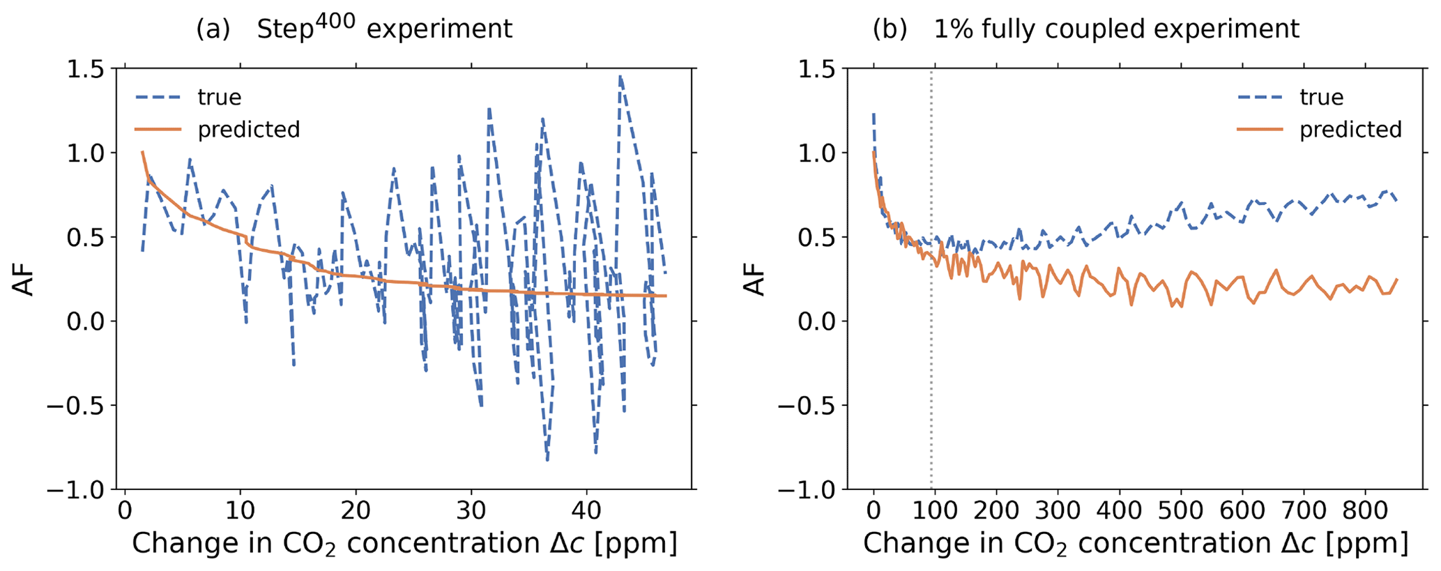
In this appendix we show how from α and γ sensitivities defined using separate land and ocean temperatures one can compute their analogues defined by means of a single global temperature, as claimed in the Outlook (Sect. 7). Global temperature in a model is obtained by

$$\begin{array}{}\text{(G1)}& \begin{array}{rl}\mathrm{\Delta }T& ={\displaystyle \frac{{\sum }_i{A}_i\mathrm{\Delta }{T}_i}{{\sum }_i{A}_i}}={\displaystyle \frac{{\sum }_{i\in \text{L}}{A}_i\mathrm{\Delta }{T}_i+{\sum }_{i\in \text{O}}{A}_i\mathrm{\Delta }{T}_i}{{\sum }_{i\in \text{L}}{A}_i+{\sum }_{i\in \text{O}}{A}_i}}\\ & ={\displaystyle \frac{{\sum }_{i\in \text{L}}{A}_i\mathrm{\Delta }{T}_i}{{\sum }_{i\in \text{L}}{A}_i}}{\displaystyle \frac{{\sum }_{i\in L}{A}_i}{{\sum }_i{A}_i}}\\ & +{\displaystyle \frac{{\sum }_{i\in \text{O}}{A}_i\mathrm{\Delta }{T}_i}{{\sum }_{i\in \text{O}}{A}_i}}{\displaystyle \frac{{\sum }_{i\in \text{O}}{A}_i}{{\sum }_i{A}_i}}=:\mathrm{\Delta }{T}_{\text{L}}{F}_{\text{L}}+\mathrm{\Delta }{T}_{\text{O}}{F}_{\text{O}},\end{array}\end{array}$$

where A_i and ΔT_i are the area and temperature of grid box i, i∈L and i∈O indicate sum over grid boxes on land and ocean, ΔT_L and ΔT_O are land and ocean temperatures, and F_L and F_O are the fractions of global area occupied by land and ocean.

Using a single global temperature, α is defined by

$$\begin{array}{}\text{(G2)}& \mathrm{\Delta }T=\mathit{\alpha }\mathrm{\Delta }c.\end{array}$$

Using separate land and ocean temperatures one defines

$$\begin{array}{}\text{(G3)}& {\displaystyle }\mathrm{\Delta }{T}_{\text{L}}={\mathit{\alpha }}_{\text{L}}\mathrm{\Delta }c,\text{(G4)}& {\displaystyle }\mathrm{\Delta }{T}_{\text{O}}={\mathit{\alpha }}_{\text{O}}\mathrm{\Delta }c.\end{array}$$

Plugging Eqs. (G1), (G3), and (G4) into (G2) gives

$$\begin{array}{}\text{(G5)}& \mathit{\alpha }={\mathit{\alpha }}_{\text{L}}{F}_{\text{L}}+{\mathit{\alpha }}_{\text{O}}{F}_{\text{O}}.\end{array}$$

Taking a single global temperature, γ is defined by

$$\begin{array}{}\text{(G6)}& \mathrm{\Delta }{C}_X^{\text{rad}}={\mathit{\gamma }}_X\mathrm{\Delta }T,\end{array}$$

where X denotes the carbon response over land (L) or ocean (O). Using separate land and ocean temperatures, γ can be defined by

$$\begin{array}{}\text{(G7)}& \mathrm{\Delta }{C}_X^{\text{rad}}={\mathit{\gamma }}_X^{*}\mathrm{\Delta }{T}_X.\end{array}$$

Inserting Eqs. (G3), (G4), (G6), and (G1) into (G7) gives

$$\begin{array}{}\text{(G8)}& {\mathit{\gamma }}_X={\displaystyle \frac{{\mathit{\gamma }}_X^{*}{\mathit{\alpha }}_X}{F_{\text{L}}{\mathit{\alpha }}_{\text{L}}+F_{\text{O}}{\mathit{\alpha }}_{\text{O}}}}.\end{array}$$

Since the Laplace-transformed formulation of the generalized framework is completely analogous to that of the original α–β–γ framework, Eqs. (G5) and (G8) extend straightforwardly to the respective generalized sensitivities:

$$\begin{array}{}\text{(G9)}& {\displaystyle }{\stackrel{\mathrm{̃}}{\mathit{\chi }}}_{\mathit{\alpha }}={\stackrel{\mathrm{̃}}{\mathit{\chi }}}_{\mathit{\alpha }}^{\left(\text{L}\right)}{F}_{\text{L}}+{\stackrel{\mathrm{̃}}{\mathit{\chi }}}_{\mathit{\alpha }}^{\left(\text{O}\right)}{F}_{\text{O}},\text{(G10)}& {\displaystyle }{\stackrel{\mathrm{̃}}{\mathit{\chi }}}_{\mathit{\gamma }}^{\left(X\right)}={\displaystyle \frac{{\stackrel{\mathrm{̃}}{\mathit{\chi }}}_{\mathit{\gamma }}^{(X,*)}{\stackrel{\mathrm{̃}}{\mathit{\chi }}}_{\mathit{\alpha }}^{\left(X\right)}}{F_{\text{L}}{\stackrel{\mathrm{̃}}{\mathit{\chi }}}_{\mathit{\alpha }}^{\left(\text{L}\right)}+F_{\text{O}}{\stackrel{\mathrm{̃}}{\mathit{\chi }}}_{\mathit{\alpha }}^{\left(\text{O}\right)}}}.\end{array}$$