Coherency and time lag analyses between MODIS vegetation indices and climate across forests and grasslands in the European temperate zone

Identifying the climate-induced variability in the condition of vegetation is particularly important in the context of recent climate change and plants' impact on the mitigation of climate change. In this paper, we present the coherence and time lags in the spectral response of three individual vegetation types in the European temperate zone to the influencing meteorological factors in the period 2002–2022. Vegetation condition in broadleaved forest, coniferous forest and pastures was measured with monthly anomalies of two spectral indices – normalised difference vegetation index (NDVI) and enhanced vegetation index (EVI). As meteorological elements we used monthly anomalies of temperature (T), precipitation (P), vapour pressure deficit (VPD), evapotranspiration (ETo), and the teleconnection indices North Atlantic Oscillation (NAO) and North Sea Caspian Pattern (NCP). Periodicity in the time series was assessed using the wavelet transform, but no significant intra- or interannual cycles were detected in both vegetation (NDVI and EVI) and meteorological variables. In turn, coherence between NDVI and EVI and meteorological elements was described using the methods of wavelet coherence and Pearson's linear correlation with time lag. In the European temperate zone analysed in this study, NAO produces strong coherence mostly for forests in a circa 1-year band and a weaker coherence in a circa 3-year band. For pastures these interannual patterns are hardly recognisable. The strongest relationships occur between conditions of the vegetation and T and ETo – they show high coherence in both forests and pastures. There is a significant cohesion with the 8–16-month (ca. 1-year) and 20–32-month (ca. 2-year) bands. More time-lagged significant correlations between vegetation indices and T occur for forests than for pastures, suggesting a significant lag in the forests' response to the changes in T.

1 Introduction

Vegetation is one of the main components of the terrestrial Earth, which plays an important role in regulating climate through evaporative cooling processes and carbon sequestration, among others. Hence, vegetation's presence between the atmosphere, hydrosphere and lithosphere is crucial (Zhang et al., 2017). Among different vegetation types, the major ones, which cover up to 78 % of the world's land area, are forests and grasslands (IPCC, 2019; FAO and UNEP, 2020).

Modern climate change is widespread, rapid and intensifying (IPCC, 2019). Climate change deepens the processes of land degradation through e.g. increase in rainfall intensity and flooding, heat stress, or drought frequency and severity (IPCC, 2019). The influence of climate change on vegetation, especially on forest conditions, is highlighted in several studies (Buras et al., 2020; Schuldt et al., 2020; Prăvălie et al., 2022; Yang et al., 2019; Liu et al., 2015). It has the potential to cause severe, long-term damage to forest ecosystems by increasing the frequency of extreme weather events, such as droughts, destructive windstorms and wildfires in many regions (Bryn and Potthoff, 2018; Hofgaard et al., 2012; Karlsen et al., 2017; Morin et al., 2018). That is why monitoring vegetation dynamics and precisely characterising the response of vegetation to changing climate is essential in order to maintain a sustainable environment (Tomlinson et al., 2011; Barbosa et al., 2019).

The most widely used parameter for evaluating vegetation's response to climate change is the normalised difference vegetation index (NDVI), derived from satellite remote sensing (Adole et al., 2016; Huang et al., 2021; Soubry et al., 2021; Buras et al., 2020; Barbosa et al., 2019). The NDVI is a normalised transform of the near-infrared to red reflectance ratio, which is intended to standardise vegetation index values to fall between −1 and +1 (Didan and Munoz, 2019). According to research, it is a trustworthy ecological indicator, if obtained from properly calibrated satellite-borne sensors (Huang et al., 2021). In the research of vegetation vigour, NDVI has a long history spanning 50 years, but in recent times the enhanced vegetation index (EVI) has also gained popularity. In the EVI formula the blue radiation is additionally used to stabilise the index value against variations in aerosol concentration levels (Didan and Munoz, 2019).

Spectral vegetation indices – NDVI and EVI – derived from Moderate Resolution Imaging Spectroradiometer (MODIS) data were coupled with meteorological elements in many research papers (e.g. Buras et al., 2020; Li et al., 2010; Mao et al., 2012; Mbatha and Xulu, 2018; Moreira et al., 2019; Zhu et al., 2023; Ghaderpour et al., 2023; Schuldt et al., 2020). The applied coupling methods used in these studies were often based on single and multiple linear regressions and Pearson's correlations between vegetation indices and climate elements but assuming the stationary relationship. However, the time lag in the correlation between vegetation indices and weather elements should not be disregarded. The spectral response to the influencing factor varies depending on the vegetation type – it is quicker for grasslands and agricultural lands (Moreira et al., 2019), while in the case of forests this response might be very extended in time (Barbosa et al., 2019; Carl et al., 2013), so a significant delay in correlation between vegetation condition and meteorological element can occur. For instance, elements such as temperature can influence the trees' phenological timing of the following year (Carl et al., 2013). Therefore, nowadays the wavelet coherence (WC) method is often used in order to capture the delay in the spectral response of the vegetation. This method allows us to study the multiscale and non-stationary processes over finite spatial and temporal domains (Furon et al., 2008) and hence is advantageous when compared to the Fourier transform because the latter requires stationarity (Martínez and Gilabert, 2009). The WC method has proven to be useful in geophysics and climatology, linking e.g. rainfall and the El Niño–Southern Oscillation (ENSO) index (Torrence and Webster, 1999) or rainfall and monsoon in Pakistan (Hussain et al., 2022). WC has already been used several times when coupling climatological factors such as temperature or rainfall and vegetation occurrence. The coherence of meteorological elements and grasslands, savannas and forests was researched e.g. in Brazil (Moreira et al., 2019; Barbosa et al., 2019), South Africa (Mbatha and Xulu, 2018), southern China (Zhou et al., 2022), India (Naga Rajesh et al., 2023) and Indonesia (Erasmi et al., 2009). In Europe, similar research was conducted in the Mediterranean (Ghaderpour et al., 2023). Surprisingly, the coherence between vegetation dynamics and climate elements in the temperate zone is very understudied, and the existing studies are limited in time and space (Carl et al., 2013; Zhu et al., 2022). Such research is especially important in light of recent vegetation disturbance caused by severe drought events that occurred in Europe in recent years (Buras et al., 2020; Schuldt et al., 2020).

This study aims to identify patterns in time series of three different types of vegetation (broadleaved and coniferous forests and pastures) in the temperate zone and relate them with meteorological elements and teleconnection indices using the wavelet transform (WT) and wavelet coherence (WC) methods. Thus, the main objectives of this research are (1) to identify the variability and periodic changes in time series of MODIS-based NDVI and EVI of different vegetation types and in time series of meteorological elements and teleconnection indices using the WT method and (2) to couple the NDVI and EVI vegetation indices with meteorological elements and teleconnection indices in order to determine the coherence and time lags in the spectral response of individual vegetation types to the influencing factors using the methods of WC and Pearson's correlation. The analyses are carried out for the broadleaved and coniferous forests and pastures in the temperate zone of central Europe in the period 2002–2022.

2 Materials and methods

2.1 Study area

The study area characterised by three vegetation types – the two types of forest (broadleaved and coniferous forest) and pastures including meadows and other permanent grasslands under agricultural use – is located in the administrative borders of Poland (Fig. 1). The analysed vegetation types are situated within a territory extending from 49 to 54.5° N latitude and from 14 to 24° E longitude. From the north, the research area borders the Baltic Sea, while the terrain changes towards the south – there are mountains at the southern edges of the research area. Because Europe's land relief is arranged mostly latitudinally, there are no orographic barriers, and climate in the study area is influenced by the western transfer of air masses and therefore indirectly by the Atlantic Ocean. The warm temperate climate is characterised by mean winter temperature from −3.5 °C (in the north-east and in the sub-mountain and foothill regions in the south) to 1.5 °C (in the west), mean summer temperature from 14.5 °C (in foothill regions in the south) to 19.5 °C (in the centre) and a mean annual precipitation from 450 mm in the centre of the study area to 1200 mm in the mountains (1991–2020) (Tomczyk and Bednorz, 2022).

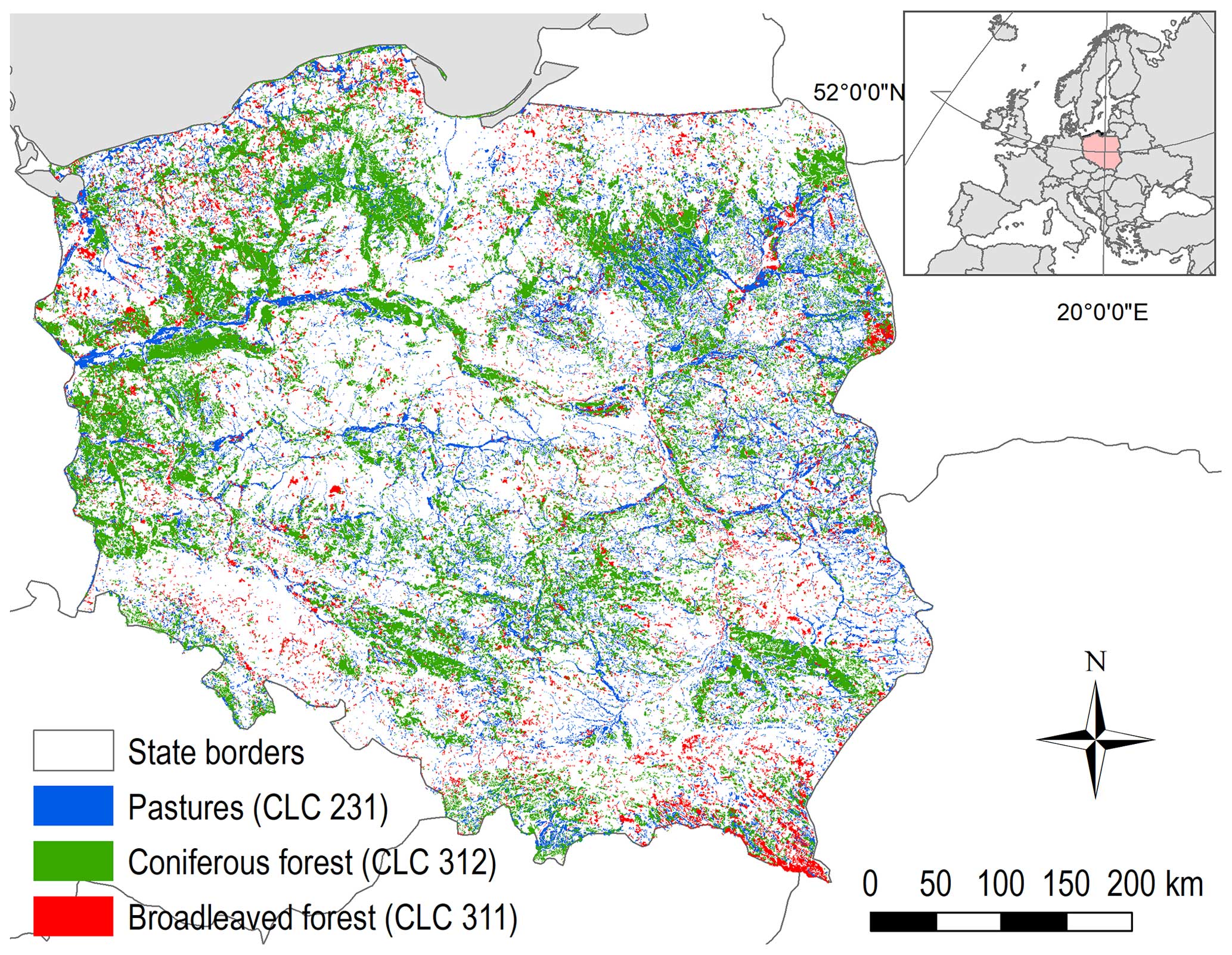
Figure 1 Spatial distribution of three vegetation masks – broadleaved forest (CLC class 311), coniferous forest (CLC class 312) and pastures (CLC class 231) – used in the study.

The selected vegetation types were defined on the basis of Corine Land Cover (CLC) 2006, 2012 and 2018 databases (CLMS, 2021). The CLC database provides data on land cover across 44 classes in European countries. For areal phenomena, the CLC employs a minimum mapping unit (MMU) of 25 ha and for linear phenomena a minimum width of 100 m. (CLMS, 2021). The CLC 2006, 2012 and 2018 databases were used to prepare masks for broadleaved forests (CLC class 311), coniferous forests (CLC class 312) and pastures (CLC class 231). The CLC forest vector layers for 2006, 2012 and 2018 were intersected, and the polygons that were still forest for these three periods made up the broadleaved or coniferous forest mask. The percentage of forest coverage was calculated for each MODIS pixel. The pixels containing at least 80 % of forest cover were selected for further analysis. To ensure the uniformity of forest pixels, a criterion of 80 % coverage of broadleaved or coniferous forest was applied. Following these selection criteria, 174 243 pixels were retained as the broadleaved forest mask and 798 777 pixels were retained as the coniferous forest mask, representing the area of 10 890 and 49 924 km², respectively. Clusters of broadleaved forest are rather small, and most of them are located in the north-western part of the study area, in the south-eastern edge of the area (Bieszczady Mountains) and in the eastern part (Białowieża Forest). The tree species dominating in the species composition are birch, oak and beech (Zajączkowski et al., 2022). In contrast, coniferous forest prevail in most of the study area, and the predominant species, covering 58 % of the forest area, is pine (Zajączkowski et al., 2022). In the mountains, the proportion of spruce and fir species composition is also apparent (Zajączkowski et al., 2022).

The pastures mask was prepared following the same steps as used for forest masks, except that only CLC vector layers for 2012 and 2018 were used (because of the poor quality of the 2006 CLC class 231). Following such selection criteria, 338 193 pixels were retained as the pastures mask, representing the area of 21 137 km².

2.2 MODIS data: NDVI and EVI

This study uses two vegetation indices (VI) – the normalised difference vegetation index (NDVI) and enhanced vegetation index (EVI) – derived from the Moderate Resolution Imaging Spectroradiometers (MODIS) on board the Terra and Aqua satellites – products MOD13Q1 and MYD13Q1 (Didan, 2021a, b). Theoretical description of the MODIS VI and the NDVI and EVI algorithm details are provided in Didan and Munoz (2019). The MOD13Q1 and MYD13Q1 products were downloaded for the period 2002–2022. Because the data from Terra and Aqua are processed 8 d out of phase at 16 d intervals, combining both satellites' data streams produces a quasi-8 d product time series (Didan and Munoz, 2019). MOD13Q1 and MYD13Q1 products are published with 250 m spatial resolution. To cover the area between 49 and 55° N latitude and 14 and 24° E longitude, three granules were required because each granule has 4800×4800 pixels. Eventually, 2712 granules were needed to cover the time period 2002–2022.

Together with the NDVI (or EVI) product, the corresponding pixel reliability and day-of-year layers were used. Because in 16 d composite the adjacent selected pixels may originate from different days, so for each pixel in such composite the day-of-year layer keeps the information about the actual day the pixel originated, while the pixel reliability layer keeps the information that describes overall pixel quality (Didan and Munoz, 2019). Based on this, only the pixels indicated as good or marginal quality were selected, which is a common practice in similar studies (e.g. Buras et al., 2020). In the next step, based on the day-of-year information, each of the selected pixels was allocated to the respective month. To get the monthly values of NDVI (or EVI), a monthly maximum NDVI (or EVI) was calculated for each of the retained pixels. The reason behind this approach is that low-value observations either are erroneous or have reduced vegetation vigour for the time period under consideration (Holben, 1986).

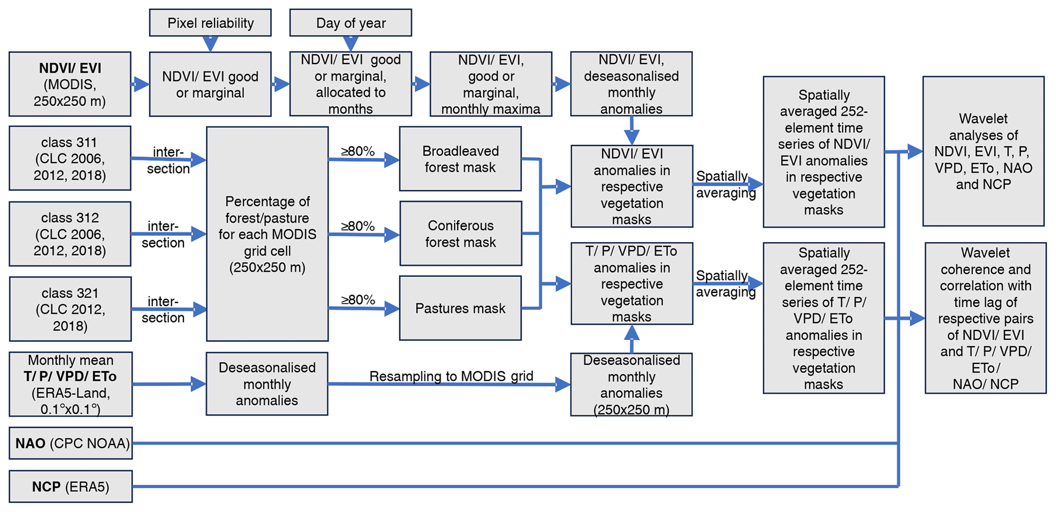
Next, the deseasonalised time series of monthly anomalies from the multi-annual monthly values of NDVI (or EVI) were prepared for each MODIS grid cell (i.e. each pixel), so that e.g. the deseasonalised value (anomaly) for January 2002 is the difference between the January 2002 value and multi-annual mean from all Januaries. It should be noted that the term “anomaly”, which is commonly used in climatological studies (e.g. Kulesza, 2021), should be interpreted as a “deviation from the mean value”. Finally, spatially averaged 252-element (21 years × 12 months) time series of NDVI (or EVI) anomalies in respective vegetation masks were prepared. The spatially averaged values of NDVI (or EVI) were calculated as area averages of all NDVI (or EVI) values in the MODIS grid cells (i.e. all pixels) within the respective vegetation masks. The methodology diagram showing the above-described steps is presented in Fig. 2.

2.3 Meteorological elements

In this work, the gridded data from ERA5-Land reanalysis (Muñoz-Sabater, 2019; Muñoz-Sabater et al., 2021) were used. The monthly data representing meteorological elements, which are generally known to have a significant impact on the dynamics of vegetation productivity (Chu et al., 2019; Liu et al., 2015; Yang et al., 2019), i.e. 2 m temperature (T, in °C), precipitation (P, in mm) and evapotranspiration (ETo, in mm), were downloaded for the period 2002–2022. Spatial extent of the meteorological data was 49 to 55° N latitude and 14 to 24° E longitude, and the resolution of reanalysis data was 0.1°×0.1°. Additionally, monthly data on 2 m dew point temperature were downloaded in order to calculate the water vapour pressure deficit (VPD, in hPa), a variable frequently used to explain the tree mortality (Gazol and Camarero, 2022; Schuldt et al., 2020). VPD is the difference between saturation vapour pressure (SVP, which is temperature-dependent) and actual vapour pressure (AVP, which is dew-point-temperature-dependent). SVP can be approximated from the air temperature records following Tetens' formula (American Meteorological Society, 2023),

$$\mathrm{SVP}=\mathrm{6.11}\times {\mathrm{10}}^{\left(\frac{\mathrm{7.5}T}{\mathrm{237.7}+T}\right)},$$

and AVP can be calculated from the same equation using dew point temperature instead of air temperature. Eventually, VPD = SVP−AVP.

In the next step the deseasonalised time series of monthly anomalies from the multi-annual monthly mean values of T, P, VPD and ETo were prepared for each grid cell of the ERA5-Land reanalysis. As in the case of NDVI (or EVI), the term “anomaly” should be interpreted as a “deviation from the mean value”. The data were then resampled to fit the MODIS grid cells (which does not affect much the data accuracy because monthly mean values of meteorological elements are slowly changing over space). Finally, spatially averaged 252-element time series of T, P, VPD and ETo anomalies in respective vegetation masks were prepared. The methodology diagram showing the above-described steps is presented in Fig. 2.

Figure 2 Flow chart of the input data and the methodology used in this paper.

2.4 Teleconnection indices

This study uses two well-known teleconnection indices: North Atlantic Oscillation (NAO) and North Sea Caspian Pattern (NCP). These large-scale climatic oscillations can be considered a proxy for the general atmospheric circulation pattern, giving aggregated information about the meteorological condition in a given year (e.g. drought-favouring conditions). The relationship between teleconnection indices and vegetation condition in different regions of the world was the focus of several studies (Brown et al., 2010; Gong and Shi, 2003; Vicente-Serrano and Heredia-Laclaustra, 2004; He et al., 2022; Gouveia et al., 2008; Olafsson and Rousta, 2021). According to many research results, NAO is associated with NDVI at higher latitudes in parts of the Northern Hemisphere (Vicente-Serrano and Heredia-Laclaustra, 2004; Olafsson and Rousta, 2021; Gouveia et al., 2008), while the NCP is associated with vegetation conditions in western Eurasia (He et al., 2022).

Monthly values of NAO index in the period 2002–2022 were downloaded from the Climate Prediction Center of the National Oceanic and Atmospheric Administration (https://www.cpc.ncep.noaa.gov/products/precip/CWlink/pna/nao.shtml, last access: 4 March 2023). The procedure used to calculate the NAO teleconnection index is based on the rotated principal component analysis (RPCA) (Barnston and Livezey, 1987). The RPCA technique is applied to monthly mean standardised 500 geopotential height anomalies in the region 20 to 90° N (and all longitudes) between January 1950 and December 2000. The anomalies are standardised by the 1950–2000 climatology. In the positive phase of NAO the westerly circulation of the atmosphere prevails over central and northern Europe, resulting in relatively warm and humid weather in winter, while there is cool and rainy weather in summer. In the negative phase, the meridional circulation occurs more often, and central Europe can then be reached by cold and dry air masses from the north or hot air masses from the south.

The NCP index was calculated on the basis of 500 geopotential height monthly values derived from ERA5 reanalysis (Hersbach et al., 2020) in the same period 2002–2022. The NCP index values were calculated from the normalised 500 geopotential height difference values between averages of North Sea (55° N, 0° and 55° N, 10° E) and northern Caspian Sea (45° N, 50° E and 45° N, 60° E) regions (Kutiel et al., 2002). In the negative phase, above-normal temperatures and below-normal precipitation occur in the Balkans, western Türkiye and the Middle East. In the positive phase, it is the other way round. There is no significant correlation between the NCP and NAO (Araghi et al., 2019).

2.5 Methods

2.5.1 Wavelet analysis

The wavelet transform (WT) was applied to the deseasonalised time series of NDVI, EVI, T, P, VPD and ETo, as well as NAO and NCP, in searching for potential variations in frequency and time at different scales. To this end, the wavelet packet (Torrence and Compo, 1998) implemented in the MATLAB computing environment was used. The use of wavelet analysis gives the information on fluctuations which change frequency over time. This is possible thanks to using wavelets – structures that are time-limited and consist of several short oscillations. The basic wavelet can be stretched and shifted in time in order to create a so-called wavelet family – a collection of similar structures. Wavelet analysis is based on correlating the individual elements of wavelet family with values of the time series throughout the observation period. The wavelet power spectrum – $|W{|}^{\mathrm{2}}$ – represents this correlation. The higher the power is, the more similar the wavelet will be to the empirical data at a given point in the time series, which means that fluctuations in a given frequency are more likely to occur in a given period. In this paper, we used the Morlet wavelet and assessed the statistical significance of the $|W{|}^{\mathrm{2}}$ values with the χ2 test (Torrence and Compo, 1998) (the level of significance α=0.05). The regions of the wavelet power spectrum, which are especially vulnerable to adverse edge effects (because of the finite length of the time series), are delimited by the “cone of influence” (COI). The values of the wavelet power spectrum which are outside of the COI are considered uncertain.

2.5.2 Wavelet coherence and time lags

In order to determine the correlations changing over time between NDVI (or EVI) and meteorological elements and teleconnection indices, the wavelet coherence (WC) was applied to the deseasonalised time series of respective data sets, resulting in six diagrams (scalograms) for each of the vegetation types for NDVI (for EVI likewise): NDVI with T, NDVI with P, NDVI with VPD, NDVI with ETo, NDVI with NAO and NDVI with NCP. Wavelet coherence combines the advantages of wavelet analysis and Pearson correlation, allowing for searching for correlations that vary over frequency and time (Torrence and Webster, 1999; Grinsted et al., 2004). In this paper, WC was prepared according to Grinsted et al. (2004) in the MATLAB computing environment. In the WC scalogram the colour scale ranges from blue (low correlation) to red (high correlation) and thus represents the wavelet coherence coefficient. The direction of arrows indicates the phase delay between signals (time series): right arrows indicate that the series are completely in phase, i.e. positive correlations, while the left arrows indicate that the series are completely out of phase, i.e. negative correlations. The statistical significance of values of the wavelet coherence coefficient was assessed using the Monte Carlo method at the significance level of α=0.05 (Grinsted et al., 2004).

In order to additionally investigate the delays in the spectral response of the individual vegetation type to the triggering meteorological factors, the overall, linear correlations with appropriate time lags were calculated. The correlated pairs of data sets were prepared with a 0- to 36-month delay (3 years). A 0-month delay means that the independent variable's values (T, P, VPD, ETo, NAO, NCP) from month i were correlated with the dependent variable's values (NDVI, EVI) from the same month. In turn, a 1-month delay means that the independent variable's values from month i were correlated with the dependent variable's values from the i+1 month, and so on. The strength of the correlation between the deseasonalised time series of NDVI (or EVI) and meteorological elements and teleconnection indices for three vegetation types was assessed using the Pearson correlation coefficient, expressed by the following formula: $r={\mathrm{cov}}_{xy}/S_x{S}_y$, where cov_xy is the covariance in the bivariate distribution of the variables x (time series of a respective meteorological element or teleconnection index) and y (time series of NDVI or EVI), and S_x and S_y are the standard deviations in the marginal distributions of the variables x and y, respectively. The significance of linear correlations calculated in this way was assessed at the significance levels of α=0.05.

3 Results

3.1 Basic characteristics of VI and meteorological elements

In the last 2 decades a slightly positive trend in condition of the forests in Poland was noticed, with a mean NDVI increase of $\mathrm{0.088}\times {\mathrm{10}}^{-\mathrm{3}}$ per year (2002–2021) (Kulesza and Hościło, 2023). The biggest increase in mean annual NDVI (by 0.030 in 20 years) was observed in central-eastern Poland, while it was weaker in the southern, western and northern edges of the study area. In turn, the biggest mean annual NDVI was observed in forests of the foothill regions in the south and also in the Baltic Sea coastal region, while central regions had lower NDVI. In general, broadleaved forests had slightly bigger mean NDVI (0.841) than coniferous forests (0.791).

The trend of mean annual T was positive over the entire research area, resulting in the increase in T by 1 to 1.6 °C (in southern and eastern regions) (2002–2021) (Kulesza and Hościło, 2023). In central and eastern regions the statistically significant increase in ETo was also reported, with a mean increase of 1.79 mm per year (while mean annual ETo is ca. 600 mm). The slope of the trend in changes in P was insignificant in the whole study area. For the detailed analysis of the spatiotemporal variability and trends in NDVI and T, P and ETo over Poland in the last 2 decades, the reader is referred our previous paper (Kulesza and Hościło, 2023).

The course of the monthly anomalies of NDVI during the period 2002–2022 showed the dynamics of three vegetation types. Positive anomalies of NDVI in the growing season (April–September) were noticeable in 2011, 2013, 2016 and 2021, whereas the negative anomalies of NDVI occurred in the growing season of 2003, 2008, 2018, 2019 and 2022 (Fig. 3). In 2015, the negative peak of NAO index in July caused the positive T anomaly, negative P anomaly and very big negative VPD anomaly (i.e. bigger-than-average deficit of water vapour) in August. In turn, all this resulted in negative values of pastures' NDVI in August and September of 2015, but forest condition seemed unaffected. In 2018, the combined effect of above-average T (in warm half-years) and mostly below-average P resulted in gradually decreasing values of NDVI in the growing season. Yet, the decrease in NDVI values was not big. Additionally, the generally positive T anomaly and negative P anomaly in the growing season of 2018 resulted in big negative VPD anomaly (i.e. deficit of water vapour bigger than average) and big positive anomaly of ETo. The following year (2019) experienced similar meteorological conditions (although not so severe), but the vegetation condition during the growing season was significantly below average. Unlike in 2018, when the NAO phase was positive in the growing season, in 2019 the NAO phase was negative during the whole growing season. Moving forward, the year 2021, probably because of the above-average P in April, May and August, experienced the positive anomalies of vegetation condition for all three types of vegetation. In contrast, the following year (2022) experienced the negative anomalies of NDVI values, especially visible at the beginning of the growing season (April–May) and especially severe for pastures. In March, May and June 2022, there were significant negative anomalies of P and VPD, together with positive anomalies of ETo.

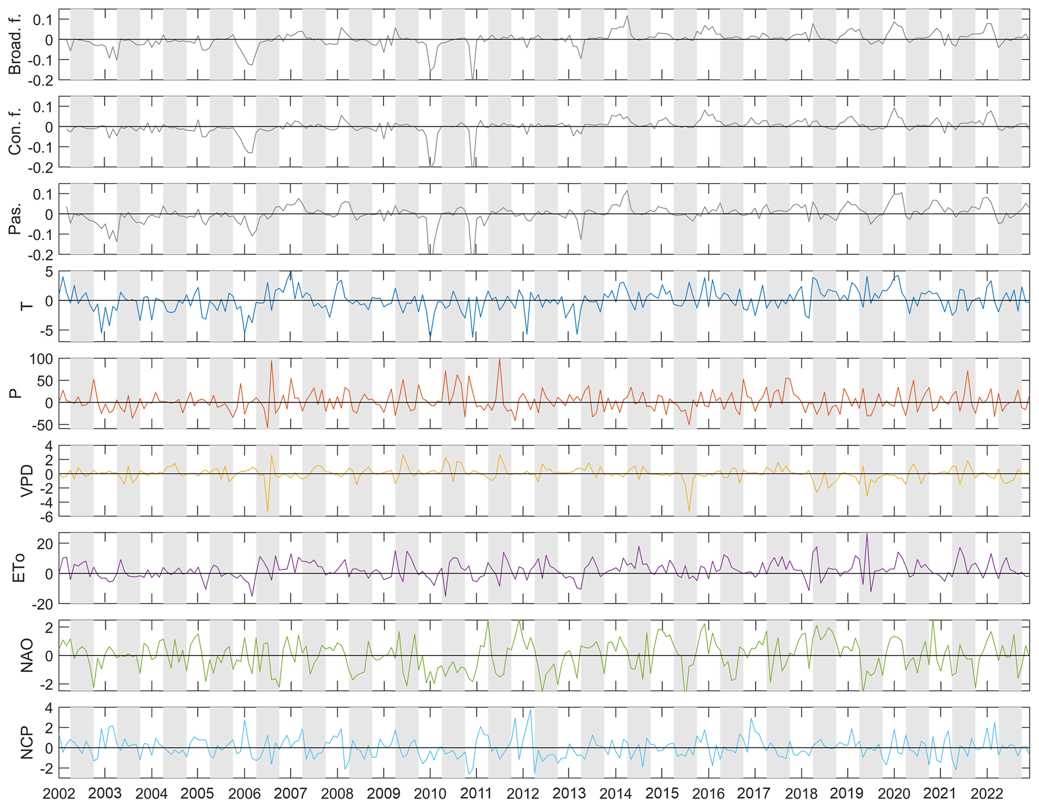
Figure 3 The deseasonalised time series of monthly anomalies of NDVI (broadleaved forest, coniferous forest, pastures), T, P, VPD, ETo, and NAO and NCP indices in the period 2002–2022. Grey areas refer to warm half-years (April–October).

3.2 Variability and periodic changes in VI and meteorological elements and teleconnection indices

The data sets used in the study were purposely deseasonalised, so the obvious 1-year cycle in both NDVI (or EVI) and meteorological conditions is removed. Thus, WT was used in searching for cycles and fluctuations with lower or higher frequency over time (i.e. interannual or intraannual cycles). Consequently, no strong and stable cycles over time are detected in the graphs which show the wavelet power spectrum $|W{|}^{\mathrm{2}}$ (Figs. 4 and 5). The pulse of a half-year and 1-year cycle of fluctuations in NDVI is marked around 2010 for all three types of vegetation (Fig. 4, left column). Although they are statistically significant, neither is the power spectrum strong, nor did they last long. The EVI shows a similar pattern for pastures but much fewer statistically significant fluctuations for broadleaved and coniferous forests (Fig. 4, right column). These pulses come from the big negative NDVI and EVI anomalies in January and December 2010 (Fig. 3), caused by extensive and persistent snow cover that significantly changed the values of spectral reflectance.

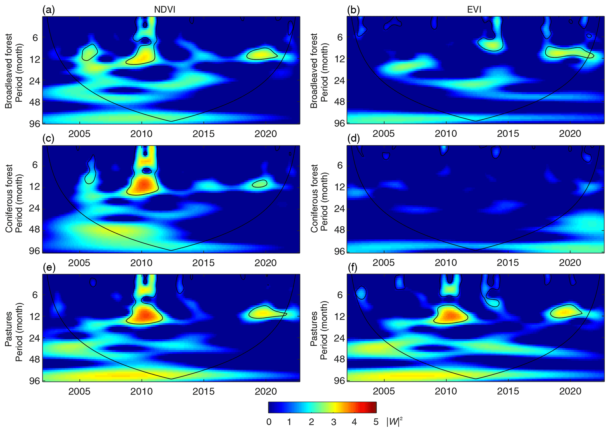
Figure 4 Wavelet power spectrum ($|W{|}^{\mathrm{2}}$) for deseasonalised time series of NDVI (a, c, e) and EVI (b, d, f) for different vegetation types during the period 2002–2022. The COI region is below the thick black line. Statistically significant areas at the level of α=0.05 are indicated by a thin black line.

Meteorological elements also do not show significant interannual cycles. The components with a period of less than half a year are more visible, but, similar to the case of NDVI, although they are statistically significant, the power spectrum is rather weak (Fig. 5). Only VPD shows a cyclical component of circa 4 years, but it lies partly in the COI region and is statistically insignificant. NAO and NCP produce significant components with a period of less than half a year (weak power spectrum) and additionally a short pulse of a 1-year cycle that is visible around 2011 (NAO and NCP) and 2015 (NAO only) (Fig. 5, lower panel).

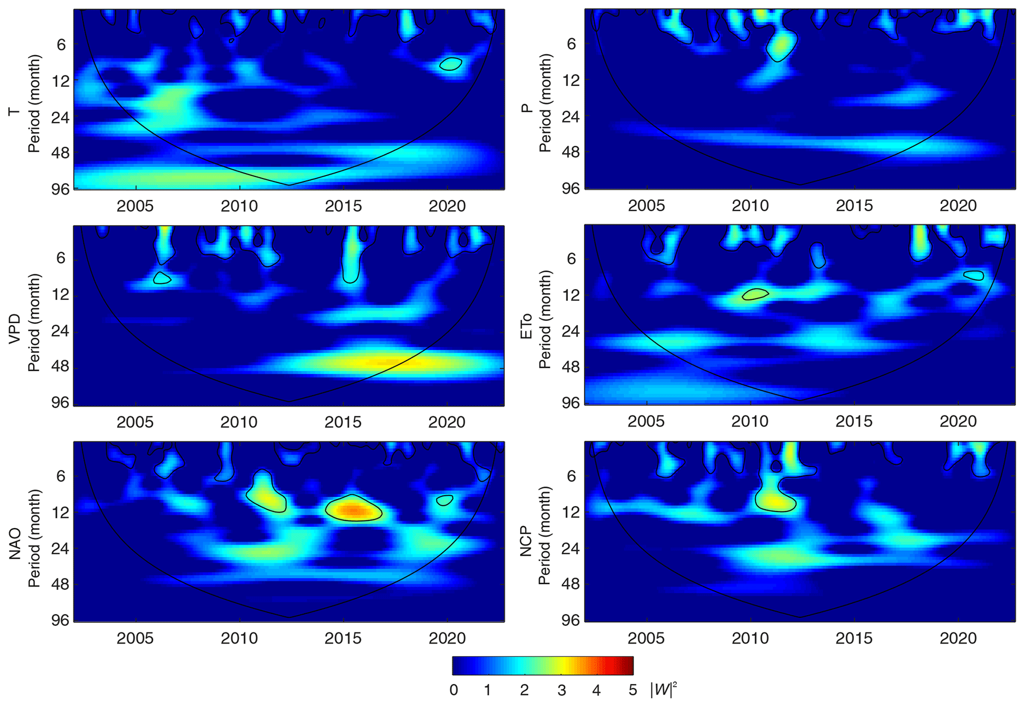
Figure 5 Wavelet power spectrum ($\left|W{|}^{\mathrm{2}}\right)$ for deseasonalised time series of T, P, VPD, ETo (mean value from three vegetation masks), and NAO and NCP during the period 2002–2022. The COI region is below the thick black line. Statistically significant areas at the level of α=0.05 are indicated by a thin black line.

3.3 Coherence and time lags in the spectral response of individual vegetation types to the influencing factors

The pattern observed for coherence between NDVI and meteorological elements and teleconnection indices is different for each of these factors.

T shows high coherence with the NDVI in all three types of vegetation. There is a significant common power in the 8–16-month (circa 1-year) band for the periods 2010–2015 and 2020–2022 (Fig. 6). The second significant common power band is 20–32 months (circa 2 years), visible for both forest types for the whole time period 2002–2022 (and for pastures only up to 2016). The observed regularities are additionally proven by the Pearson linear correlations with appropriate time lags. Significant positive correlations between NDVI and T occur for broadleaved and coniferous forests for 8-, 12-, 27-, 28-, 29- and 30-month delays (Fig. 8). For pastures significant positive correlations between NDVI and T only occur for 12- and 27-month delays.

Both P and VPD produce a few small patches of significant coherence with NDVI in all three vegetation types. Very small patches of high coherence in the circa 1-year band between NDVI and P occur only around 2006 and 2009–2010 for broadleaved and coniferous forests (and for pastures only one patch around 2009–2010) (Fig. 6). VPD produces even smaller patches of high coherence in the circa 8-month band (around 2006), where the NDVI and VPD are mostly out of phase, meaning that the correlation between them is negative (Fig. 6). In fact, significant negative Pearson's correlations appear for 7-, 8- and 9-month delays for all vegetation types (Fig. 8). Figure 8 indicates also significant correlations between NDVI and VPD for 18- and 22-month delays.

ETo shows high coherence with NDVI in all three vegetation types. The significant common power appears in the intraannual (3–8-month) band from the beginning of the study period until 2008 (Fig. 6). High and significant coherence in a circa 1-year (8–16-month) band occurs mostly around 2010, while significant coherence in the circa 2-year (20–32-month) band is distributed more or less along the whole study period. Surprisingly, it seems the most stable for pastures, which is low grassy vegetation, rather independent from interannual weather conditions. Significant positive Pearson's correlations between NDVI and ETo occur for broadleaved and coniferous forests for 8- and 22-month delays, while for pastures only for the 22-month delay (Fig. 8).

Correlations in specific bands – intraannual and interannual – are also visible between NDVI and the NAO index in particular time periods. NAO produces strong coherence with NDVI mostly for two forest types. Small areas of high positive correlation in the circa 1-year band between NDVI and NAO appear mostly for coniferous forest in the period 2013–2016 and 2018–2021, as well as for broadleaved forest in the period 2015–2016 and 2019–2020. This is additionally proven by the significant positive Pearson's correlation between NDVI and NAO for the 11-month delay (Fig. 8). For pastures this interannual pattern is hardly recognisable (Fig. 6). For broadleaved and coniferous forests the coherence in the circa 3-year band up till 2013 is also visible. Interestingly, there is a significant common power for NDVI and NAO in the 2–6-month (intraannual) band for the year 2018 in all three vegetation types. Similar small patches of high and significant intraannual coherence for this year are mostly visible for broadleaved forest regarding T, VPD and ETo but for coniferous forest and pastures regarding ETo only (Fig. 6).

The NCP index produces a rather weak coherence with NDVI in all three vegetation types. The cohesion pattern is somehow similar to the one produced by NAO, with small areas of high and significant coherence in the circa 1-year band around 2015 and 2020, which is mostly visible for coniferous and broadleaved forests (Fig. 6). Additionally, for two forest types the coherence of circa 32 months (almost 3 years) in the period 2010–2015 is also visible. Surprisingly, NCP's Pearson's correlation with NDVI is significant for the 25- and 35-month delays (for forest types), but, unlike the cohesion's right arrows, this correlation is negative (Fig. 8).

The pattern observed for coherence between EVI and meteorological elements and teleconnection indices resembles in many places the pattern observed for NDVI, especially regarding pastures.

However, in forest types, concerning T and ETo, their coherence with EVI gives substantially smaller areas of high and significant cohesion, as compared to NDVI (Fig. 8). Nevertheless, the Pearson linear correlations with time lags, prepared for EVI, reveal many significant and positive correlations between EVI and T for broadleaved forest (mostly 1-year delay and 2-year delay) and even more significant correlations for coniferous forest. In turn, significant positive Pearson's correlations between EVI and ETo occur in broadleaved forest for a circa 2-year (22-month) delay but in coniferous forest for a circa 1-year (10-month) delay and a 2-year (22- and 23-month) delay (Fig. 8).

P and VPD show some more areas of significant common power with EVI than with NDVI, but the high-cohesion areas are in an over 3-year band and lie partly in the COI region (Fig. 8).

In the case of NAO, there is a significant common power with EVI in the 30–40-month (circa 3-year) band in the period 2005–2020 for broadleaved forest (Fig. 7). This is additionally proven by the Pearson linear correlations with 30-month time lag (Fig. 8). Similar to the case of NDVI, there is a significant common power for EVI and NAO in the 2–4-month (intraannual) band for the year 2018 for both forest types. Similar small patches of high and significant intraannual coherence for this year are visible for broadleaved and coniferous forest regarding T, VPD and ETo (Fig. 7).

NCP shows fewer areas of significant common power with EVI than with NDVI. However, there are some significant positive Pearson's correlations between EVI and NCP, but there are also significant negative correlations (30-month delay for broadleaved forest) (Fig. 8). Moreover, unlike other meteorological variables, here the arrows on the WC scalograms tend to orientate up or down, which could be interpreted as uncoupling between both signals (Fig. 7).

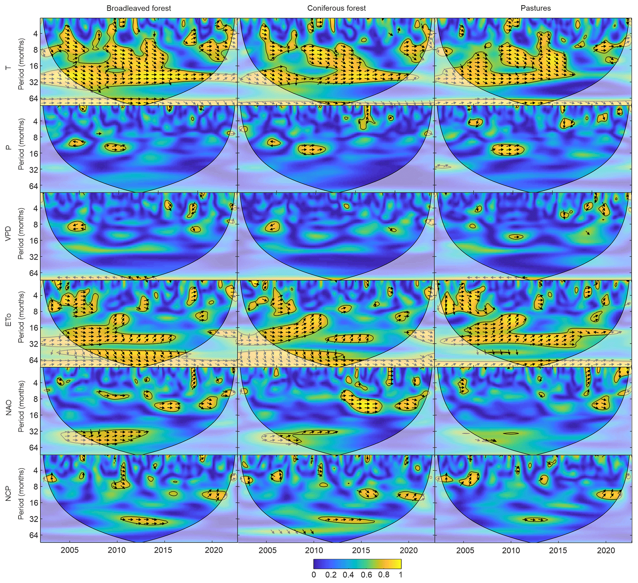
Figure 6 Wavelet coherence power spectrum (colour scale) between deseasonalised time series of NDVI and T, P, VPD, ETo, NAO and NCP for broadleaved forest (left column), coniferous forest (middle column) and pastures (right column) during the period 2002–2022. Colours range from blue (low correlation) to yellow (high correlation). Arrows indicate the phase difference between signals: right arrows – series are completely in phase; left arrows – series are out of phase. The COI region is below the thick black line. Statistically significant areas at the level of α=0.05 are indicated by a thin black line.

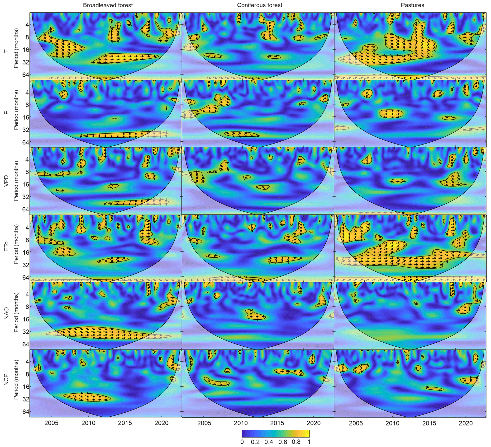
Figure 7 Wavelet coherence power spectrum (colour scale) between deseasonalised time series of EVI and T, P, VPD, ETo, NAO and NCP for broadleaved forest (left column), coniferous forest (middle column) and pastures (right column) during the period 2002–2022. Colours range from blue (low correlation) to yellow (high correlation). Arrows indicate the phase difference between signals: right arrows – series are completely in phase; left arrows – series are out of phase. The COI region is below the thick black line. Statistically significant areas at the level of α=0.05 are indicated by a thin black line.

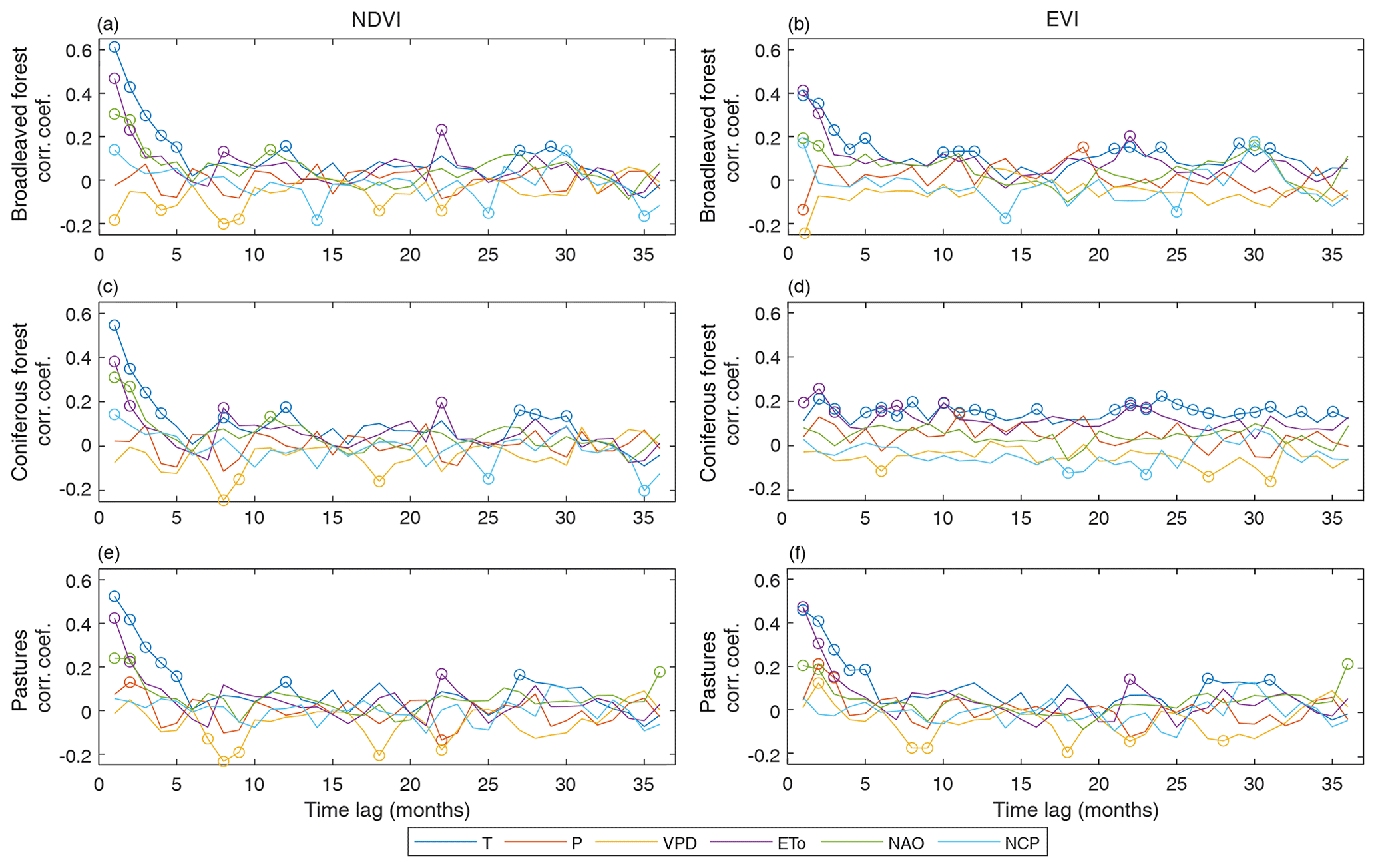
Figure 8 Correlation coefficients between deseasonalised time series of NDVI (a, c, e) or EVI (b, d, f) and T, P, VPD, ETo, NAO and NCP for three different vegetation types: broadleaved forest (a, b), coniferous forest (c, d) and pastures (e, f). The pairs of data sets are correlated with appropriate time lags of 0 to 36 months. Statistically significant correlations at the level of α=0.05 are indicated by a circle.

4 Discussion

Observed years with decreased vegetation conditions and unfavourable meteorological conditions related to this (above-average T and below-average P) are identified in many research studies. A number of severe, large-scale drought events occurred across Europe in the last 20 years, many of which have also affected the area of this study. In 2003, a severe drought mostly affected south-western Germany, Switzerland and south-eastern France (Fink et al., 2004; García-Herrera et al., 2010) with less impact on Poland (Somorowska, 2022). As the NAO index was oscillating around zero (Fig. 3), the anticyclonic pattern that led to a drought corresponded more to anomalous northern displacement of the Azores High than a typical blocking structure (Fink et al., 2004). Yet, the key factor to reach unprecedented temperature anomalies was soil moisture deficit (Fink et al., 2004). Indeed, a peak of positive ETo was also visible in May 2003 in our study area. In turn, in 2015 the negative peak of NAO index in July caused the drought in Europe that reached its peak intensity and spatial extent in August, affecting especially the eastern part of Europe (Ionita et al., 2017). Here, a very big negative VPD anomaly occurred in August and resulted in a decreased condition of the vegetation, especially of pastures. Other severe droughts occurred in Europe in 2018 (Buras et al., 2020; Schuldt et al., 2020; Boergens et al., 2020), 2019 (Boergens et al., 2020; Hari et al., 2020) and 2022 (Buras et al., 2023; Wang et al., 2023). All of them were observed also in our study area. In summer 2018 daily maximum temperature in Poland was 3.3 °C higher than the 1981–2019 average (and 1.2 °C higher than daily maximum temperature in 2003), and precipitation was below average as well. In 2019, the negative phase of NAO, persisting for the whole growing season of 2019, contributed to anticyclonic circulation and southerly advection of the air masses over Poland. The frequency of circulation from the south and south-east direction was 2 to 2.5 times higher than the average for the 1951–2018 period (Ziernicka-Wojtaszek, 2021). As a consequence, June 2019 with a positive temperature anomaly of over 4.0 °C (Fig. 3) was the warmest month since 1951 (Ziernicka-Wojtaszek, 2021). The occurrence of the consecutive summer droughts in 2018 and 2019 was unprecedented, and its combined impact on the growing season vegetation was much stronger compared to the year 2003 (Hari et al., 2020). Indeed, the negative anomalies of NDVI were observed for all three vegetation types in 2018, but the vegetation condition during the growing season of 2019 was even more below average. It is also important to mention that increased vegetation growth at the beginning of the growing season, caused by favourable meteorological conditions, contributes to the fast depletion of resources (e.g. soil moisture) and promotes and strengthens droughts in summer (Somorowska, 2022; Bastos et al., 2020). That was the case of 2018 and 2019 too. In order to conduct the WT analysis, both NDVI (or EVI) and meteorological time series were purposely deseasonalised, so the obvious 1-year cycle, resulting from the seasonality of weather pattern and vegetation in the temperate zone, is removed. Time series of meteorological elements do not show any significant interannual cycles in the period 2002–2022. Similarly, no significant interannual cycles in meteorological time series in central Europe were found in other works using much longer time periods, regarding T (Sen and Ogrin, 2016), P (Brázdil et al., 2021; Sen and Kern, 2016) and NAO, which is rather a stochastic, unpredictable and a strong non-stationary process (Schulte et al., 2015; Pozo-Vázquez et al., 2001). Additionally, no strong and stable interannual cycles over time were detected in the deseasonalised time series of NDVI (and EVI). Thus, presumably the spectral response of the vegetation to the triggering meteorological factors is caused rather by the actual relationship between these variables than being as a result of a coincidence. The WC and Pearson's linear correlation with appropriate time lags helped reveal these relationships between NDVI (or EVI) and meteorological elements.

According to many scientific studies, temperature is one of the most influential elements, shaping the vegetation condition worldwide (Moreira et al., 2019; Ghaderpour et al., 2023; Mbatha and Xulu, 2018). The correlation between grasslands' vigour and air temperature was strong in the annual cycle in southern Brazil (2000–2014) (Moreira et al., 2019). A similar significant common power in the 8–16-month (ca. 1-year) band was produced by NDVI and soil temperature for savannas and forest in South Africa in the period 2002–2017 (Mbatha and Xulu, 2018). In Europe, significant annual in-phase coherency was observed between NDVI and land surface temperature in northern Italy in the period 2000–2021 (Ghaderpour et al., 2023). In the temperate zone analysed in this study, T shows high coherence with NDVI in both forests and pastures. There is significant cohesion with the 8–16-month (ca. 1-year) and 20–32-month (ca. 2-year) bands. Pearson's linear correlation shows more time-lagged significant correlations between NDVI (or EVI) and T for forests than for pastures. This suggests that there is a significant lag in the forests' response to the changes in T, more noticeable for forests than for pastures. It is in line with the results of other researchers. For instance, in a beech forest in Germany, a time shift of approximately 300 d appears in the WC between NDVI and T (1989–2007) (Carl et al., 2013).

Similar high coherence values are produced by ETo in both forest types and in pastures – mostly coherence in the circa 1-year (8–16-month) and circa 2-year (20–32-month) bands. Indeed, forest vegetation response to water deficit can be delayed, especially depending on the tree type (broadleaved or coniferous) and species. A similar in-phase relationship in the 8–18-month band occurred in savannas and forest in South Africa (Mbatha and Xulu, 2018). Yet, the surprisingly high coherence in the 2-year band, which occurs for pastures along the whole study period, is interesting because one would expect current low grassy vegetation to be independent of the weather conditions in the previous growing seasons. However, one should remember that in statistics, a significant correlation between two variables may occur by chance, so a significant commonality in a wavelet coherence spectrum analysis does not necessarily imply interconnection (Mbatha and Xulu, 2018).

At this point, it is also worth adding some comment on the differences in WC pattern observed for NDVI and EVI. Regarding pastures, the coherence between EVI and meteorological elements and teleconnection indices resembles (more or less) the pattern observed for NDVI, while it differs substantially when forest types are concerned. Indeed, the correlation coefficient between deseasonalised anomalies of NDVI and EVI is very high for pastures (0.94) but lower for broadleaved forest (0.67) and coniferous forest (0.28). It is also worth noticing that regarding forest, the EVI values are within a much narrower range than values of NDVI (Fig. 9), mostly because of the very low NDVI values in winter months of 2006 and 2010. The reason for this might lie in different spectral bands used to construct both indices. The research results indicate that EVI is more susceptible to changes in canopy structure, while NDVI is more sensitive to chlorophyll (Huete et al., 2002). Thus, while EVI may more accurately represent early leaf shedding, NDVI is more likely to represent changes in leaf colour, such as those occurring during premature leaf senescence during a drought (Buras et al., 2020). While some researchers suggest that NDVI reflects natural vegetation better than EVI (Li et al., 2010), others prefer the latter, which also uses blue radiation to stabilise the index value against variations in aerosol concentration levels (Didan and Munoz, 2019).

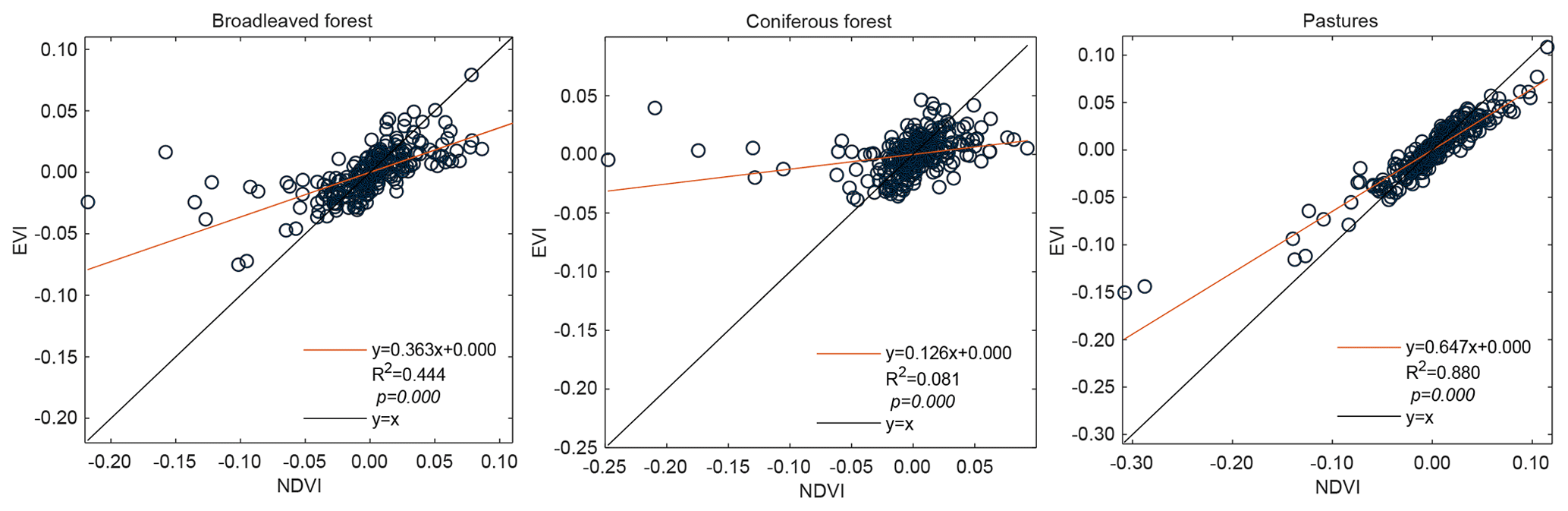
Figure 9 Scatterplots of deseasonalised anomalies of NDVI and EVI for three different vegetation types: broadleaved forest, coniferous forest and pastures. The graphs also show the linear regressions (red lines), the regression equations, the coefficient of determination R² and the statistical significance level p.

Unlike in tropical and subtropical zones, P seems to have weaker coherence with NDVI in the European temperate zone. Lotsch et al. (2003) showed that ecosystems in arid and semi-arid climate regimes (shrublands, savannas, grasslands) are most sensitive to seasonal P anomalies at timescales of 4–6 months, whereas forested land areas exhibit weak correlation with P anomalies at all timescales. According to Lotsch et al. (2003) European temperate zone lies in the area of weak correlations between P and NDVI. In southern Brazil, low coherence between EVI and P was observed only in regions where dry periods may occur during summer (thus similar to temperate zone weather conditions) (2000–2014) (Moreira et al., 2019). In Italy in 2000–2021, NDVI and P were significantly coherent only in the south, where the climate is the driest (Ghaderpour et al., 2023). In general, vegetation in the subtropical or tropical zone is more weather-dependent, leading to high coherence between vegetation vigour and P anomalies. On the other hand, the temperate forest is less dependent on water availability thanks to the deep root system that trees can use to reach deep water resources. However, it makes the influence of meteorological factors on forest NDVI/EVI less evident and harder to detect.

Another important characteristic of the vegetation in the temperate zone is that in winter vegetation mostly pauses (apart from some coniferous tree species), while meteorological elements obviously do not. P does not only show a seasonal variability (bigger sums of P occur in summer and lower in winter), but its intra- and interannual variations in winter are relatively high. The resulting coherence between NDVI and P on the monthly basis, detected on the WC scalogram, is rather weak. To compare, the NDVI correlates well with P on the yearly basis, and this correlation is much stronger than the one between NDVI and T (Kulesza and Hościło, 2023).

Drought stress on vegetation over Europe is linked also to various teleconnection patterns, with most studies focusing on the influence of NAO on vegetation condition (Gouveia et al., 2008; Olafsson and Rousta, 2021; Araghi et al., 2019). According to Gouveia et al. (2008), negative values of winter NAO induce low values of NDVI in spring but high values of NDVI in summer in north-eastern Europe. The positive phase of NAO has the opposite effect. This behaviour mainly results from the strong impact of NAO on winter temperature, associated with the critical dependence of vegetation growth on the combined effect of warm conditions and water availability during the winter season (Gouveia et al., 2008). In this study, it was especially visible in the year 2018, when the massive drought over Europe occurred. The NAO-induced stable high-pressure system formed over central Europe in April and lasted until October 2018, causing exceptionally high temperature and a big deficit of water vapour. The spectral response of the vegetation to changes in NAO index was 2–6 months delayed – and similar were the delays in response to changes in T, VPD and ETo.

However, apart from this exceptional drought of 2018, when the vegetation response to the triggering factors was relatively quick, NAO produces strong coherence with NDVI mostly for forests within the circa 1-year band and a weaker coherence within the circa 3-year band. For pastures these interannual patterns are hardly recognisable. As the atmosphere is a system of interlinked vessels, the NAO may itself be influenced by other teleconnection systems, e.g. 3–4-year cycle of ENSO (King, 2023). Thus the indirect effect of ENSO on vegetation condition in Europe might be investigated in the future.

In contrast, NCP index produces rather weak coherence with both NDVI and EVI in all three vegetation types. As there are both positive and negative (depending on the time lag) significant Pearson's correlations between NDVI (or EVI) and NCP, it seems that the overall influence of NCP on vegetation condition in the European temperate zone is rather weak. It is contrary to the results of He et al. (2022), obtained for western Eurasia for 1981–2015. They concluded that NCP has significant negative impact on meteorological and vegetation conditions over this region. According to He et al. (2022) the positive NCP phases may better contribute to drier conditions over the region than NAO because the positive phases of NCP contribute to increasing dryness, thus causing the region to become more water-limited.

Finally, it should be noted that the conducted analyses have a few limitations. In general, vegetation in warm temperate climate is highly seasonal. In the face of that, a severe weather condition occurring at the beginning of the growing season (e.g. drought) can induce poor vegetation conditions in summer and autumn. However, big positive anomalies of T or big negative anomalies of P that occur in late autumn have a much smaller influence on vegetation conditions in winter. That is why the intraannual relationships, with the time lag smaller than 1 year, are a bit harder to detect than similar relationships in the tropical or subtropical zones.

Another important issue is the interpretation of the spectral indices' values. For instance, the NDVI signal coming from forest reflects not only the trees' vigour, shaped by weather conditions, but also the “noise” from the understorey and other effects like pests, herbivores, pathogens and forest management. Grassland seems to be mostly free from such problems. Its response to the triggering meteorological factor is usually quick. Also, the quality of grassy vegetation in one year does not have a major effect on its quality in the subsequent year. In this study we only used pastures (CLC class 231) and not arable lands (CLC class 211 and 212) or natural grasslands (CLC class 321) (CLMS, 2021) to ensure the uniformity of the grassy vegetation. The natural grassland class in Poland is assigned mostly to small areas of military training grounds and alpine grassland with rough, uneven ground; steep slopes; and up to 50 % of bare rocks or bare natural surfaces (Kosztra et al., 2017). However, pastures are mowed during the growing season, which changes their spectral properties regardless of the weather. Because of this, the proper interpretation of the obtained results can be difficult. At the same time, such results should be treated with caution.

Finally, it should be noted that in this study all pixels within the respective vegetation masks were spatially averaged in order to produce single time series. However, the relationship between vegetation indices and meteorological elements may vary within each mask. Some initial sample results (illustrated in Figs. A1 and A2 in Appendix A) showed us that there are no big differences between individual parts of Poland. Poland is in fact the ninth largest country in Europe, but when it comes to response of different types of vegetation to changes in meteorological conditions, it might be considered relatively homogenous and therefore representative of the whole European warm temperate zone.

5 Conclusions

The results presented in this paper show in detail the coherence and time lags in the spectral response of three individual vegetation types in the temperate zone to the influencing meteorological factors in the period 2002–2022. Vegetation conditions in broadleaved forest, coniferous forest and pastures were measured with monthly anomalies of two spectral indices: NDVI and EVI. As meteorological elements we used monthly anomalies of T, P, VPD, ETo, and teleconnection indices NAO and NCP. Periodicity in the time series of different vegetation types and in the time series of meteorological elements and teleconnection indices was assessed using the WT method. In turn, coherence between NDVI and EVI and meteorological elements was described using the methods of WC and Pearson's linear correlation with time lag. The use of various research methods helps to objectify the results obtained.

Thanks to conducting the WT analysis, no significant and stable intra- or interannual cycles over the whole time period were detected in both vegetation (NDVI and EVI) and meteorological variables.

In the European temperate zone analysed in this study, the weakest coherence with vegetation conditions is produced by P and VPD. Also NCP produces rather weak coherence with both NDVI and EVI in all three vegetation types. In contrast, NAO produces strong coherence mostly for forests within the circa 1-year band and a weaker coherence within the circa 3-year band. For pastures these interannual patterns are hardly recognisable. The strongest relationships occur between conditions of the vegetation and T and ETo – they show high coherence in both forests and pastures. There is a significant cohesion within the 8–16-month (ca. 1-year) and 20–32-month (ca. 2-year) bands. More time-lagged significant correlations between vegetation indices and T occur for forests than for pastures, suggesting a significant lag in the forests' response to the changes in T. Yet, the surprisingly high coherence between vegetation condition and ETo in the 2-year band, which occurs for pastures along the whole study period, is interesting because low grassy vegetation seems to be unrelated to interannual weather conditions. To explain this, further in-depth research is required based on the increasingly longer research material. Additionally, as a division into just three vegetation types (broadleaved forest, coniferous forest, pastures) is rather coarse, a more detailed classification into e.g. tree species should be prepared, and the selected species-homogenous areas should be investigated in the future. The species-homogenous areas might also be further divided spatially in order to check in detail the differences in species responses to the changes in meteorological conditions in different regions of the study area.

Another important methodological conclusion is the observed differences in forest NDVI and EVI, while for pastures NDVI and EVI values seem to be very similar. Finding out which of these indicators is more suitable for which type of forest and for low grassy vegetation requires separate, extended research that should be conducted in the future.

The research presented in this study fills the knowledge gap on the coherence between vegetation conditions and meteorological elements in the temperate zone. However, the obtained results might be useful for researchers working on this topic in other climatic zones. Identifying the climate-induced variability in the condition of vegetation is particularly important in the context of recent climate change and plants' impact on mitigation of climate change.

Appendix A

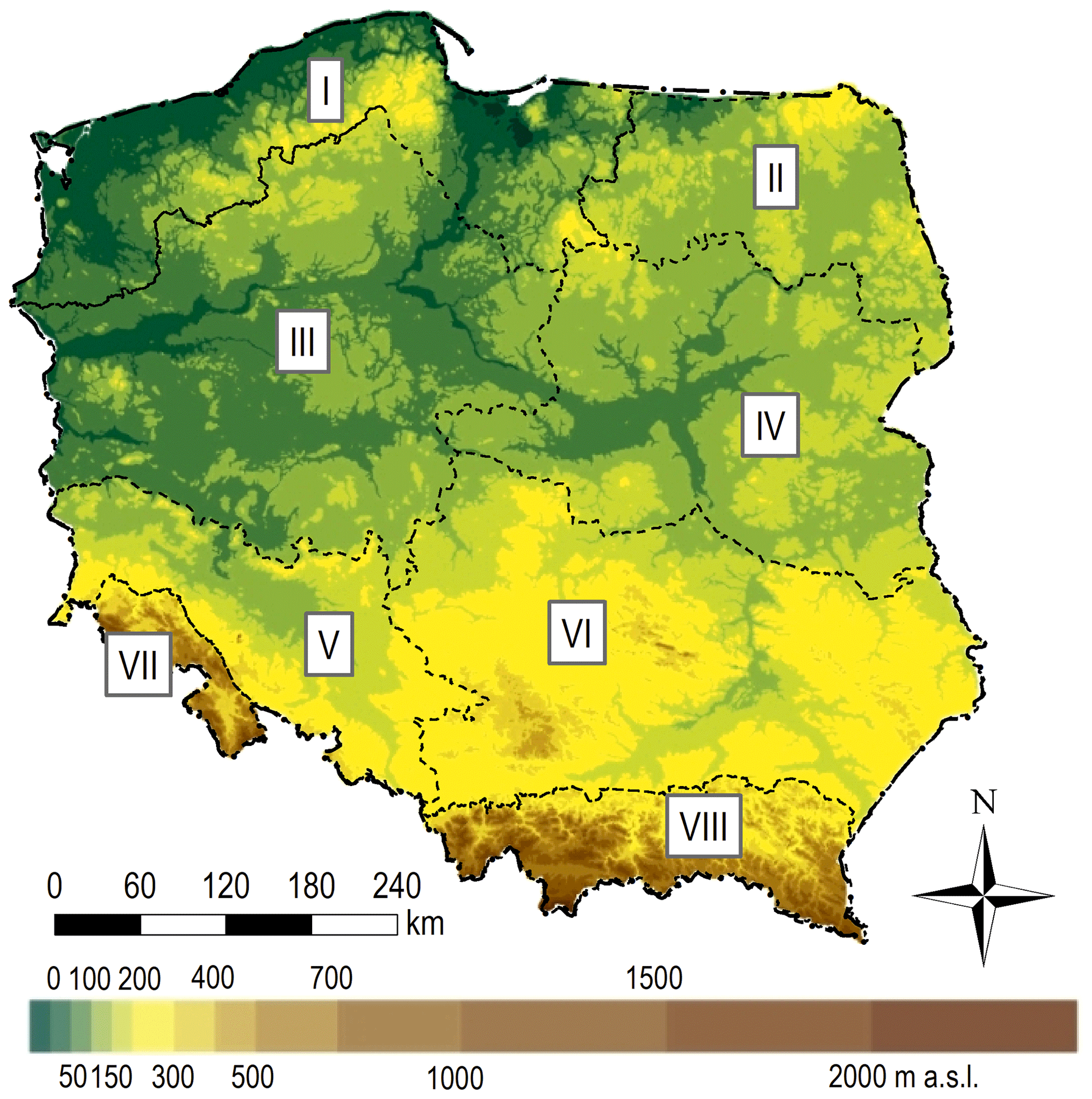
Figure A1 Hypsometric map of Poland with division into eight main nature-forest lands: I – Bałtycka, II – Mazursko-Podlaska, III – Wielkopolsko-Pomorska, IV – Mazowiecko-Podlaska, V – Śląska, VI – Małopolska, VII – Sudecka, VIII – Karpacka (source: own elaboration based on a hypsometric map, https://pl.wikipedia.org, last access: 4 November 2022).

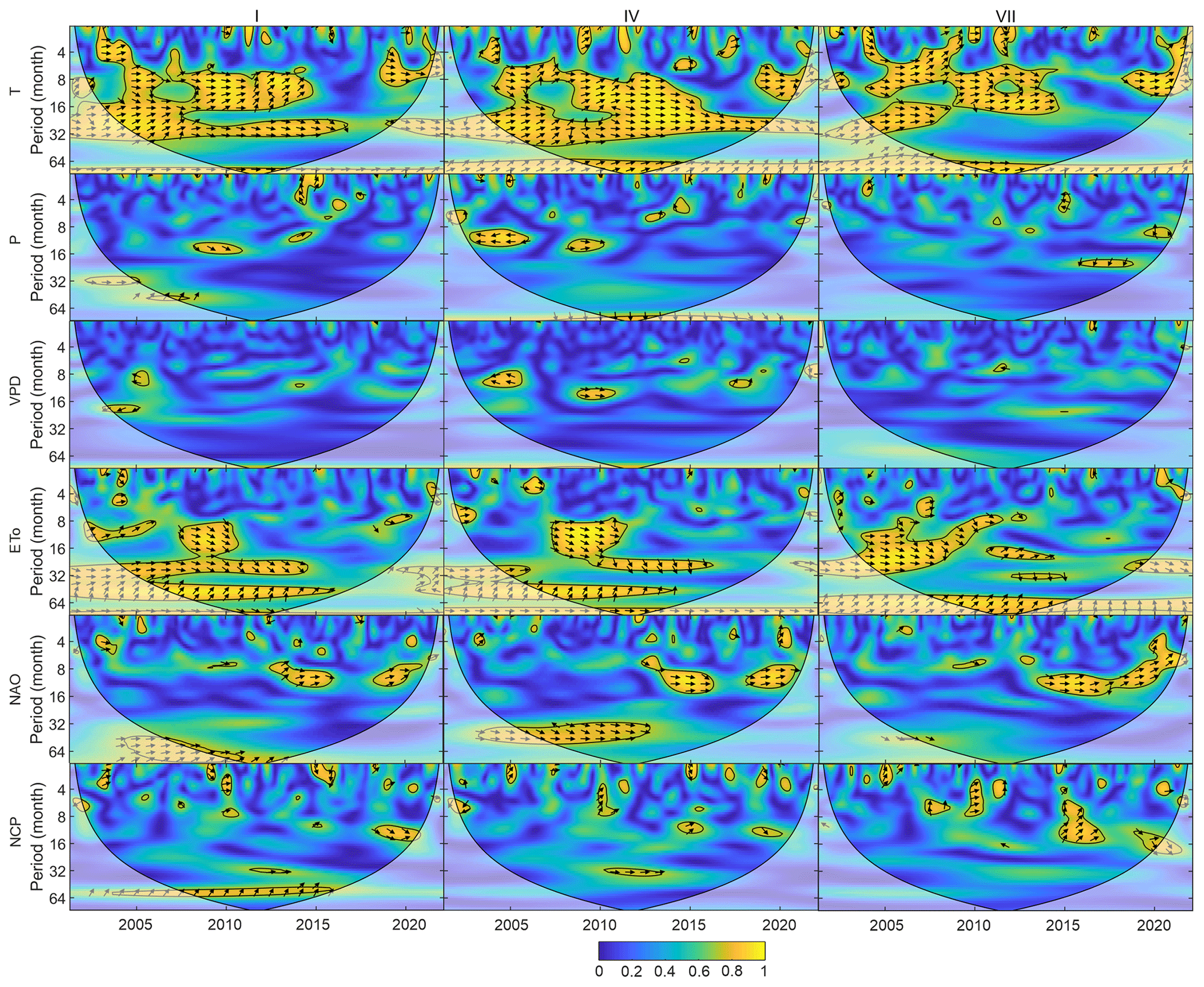
Figure A2 Wavelet coherence power spectrum (colour scale) between deseasonalised time series of NDVI and T, P, VPD, ETo, NAO and NCP for broadleaved forest in the selected three nature-forest lands: I (left column), IV (middle column) and VII (right column) during the period 2002–2022. Colours range from blue (low correlation) to yellow (high correlation). Arrows indicate the phase difference between signals: right arrows – series are completely in phase; left arrows – series are out of phase. The COI region is below the thick black line. Statistically significant areas at the level of α=0.05 are indicated by a thin black line.