Underestimation of multi-decadal global O₂ loss due to an optimal interpolation method

The global ocean's oxygen content has declined significantly over the past several decades and is expected to continue decreasing under global warming, with far-reaching impacts on marine ecosystems and biogeochemical cycling. Determining the oxygen trend, its spatial pattern, and uncertainties from observations is fundamental to our understanding of the changing ocean environment. This study uses a suite of CMIP6 Earth system models to evaluate the biases and uncertainties in oxygen distribution and trends due to sampling sparseness. Model outputs are sub-sampled according to the spatial and temporal distribution of the historical shipboard measurements, and the data gaps are filled by a simple optimal interpolation method using Gaussian covariance with a constant e-folding length scale. Sub-sampled results are compared to full model output, revealing the biases in global and basin-wise oxygen content trends. The simple optimal interpolation underestimates the modeled global deoxygenation trends, capturing approximately two-thirds of the full model trends. The North Atlantic and subpolar North Pacific are relatively well sampled, and the simple optimal interpolation is capable of reconstructing more than 80 % of the oxygen trend in the non-eddying CMIP models. In contrast, pronounced biases are found in the equatorial oceans and the Southern Ocean, where the sampling density is relatively low. The application of the simple optimal interpolation method to the historical dataset estimated the global oxygen loss to be 1.5 % over the past 50 years. However, the ratio of the global oxygen trend between the sub-sampled and full model output has increased the estimated loss rate in the range of 1.7 % to 3.1 % over the past 50 years, which partially overlaps with previous studies. The approach taken in this study can provide a framework for the intercomparison of different statistical gap-filling methods to estimate oxygen content trends and their uncertainties due to sampling sparseness.

1 Introduction

Historical observations indicate that the ocean oxygen (O₂) inventory has declined in recent decades, a trend that has been termed ocean deoxygenation (Keeling et al., 2010; Levin, 2018). Ocean heat uptake causes the reduction of oxygen solubility and changes in ocean circulation and biogeochemical processes. Ocean warming and increasing stratification can further decrease O₂ exchange between upper and deep layers, further reducing the oceanic O₂ inventory. The reduction in dissolved oxygen can have far-reaching impacts on marine habitats (Deutsch et al., 2015; Gruber, 2011; Pörtner and Farrell, 2008; Vaquer-Sunyer and Duarte, 2008).

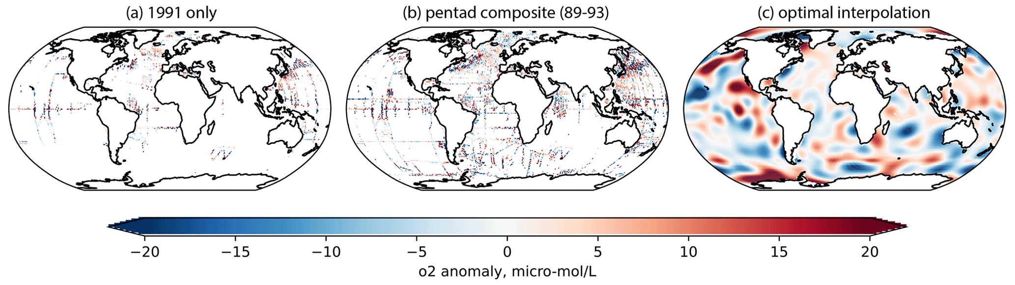
Figure 1 Maps of (a) single-year observation for the O₂ anomaly in the year 1991 at 200 m depth; (b) the pentadal composite O₂ anomaly centered in the year 1991, covering the period from 1989 to 1993, at 200 m depth; and (c) the optimally interpolated pentadal O₂ anomaly based on the data in the middle figure.

The distribution of historical O₂ measurements is irregular and sparse. The calculation of changes in the global O₂ content requires filling the data gaps in time and space, making it difficult to quantify global trends and their uncertainties. Recent estimates of the global oxygen decline are in the range of 0.5 %–3.3 % (IPCC, 2022) relative to climatological means over the period of 1970–2010 (Helm et al., 2011; Schmidtko et al., 2017; Ito et al., 2017). The wide range in the estimates of ocean deoxygenation can stem from different interpolation methods to estimate global O₂ content, different data quality control standards, and different data sources. Previous studies estimating the rates of ocean deoxygenation have relied on the World Ocean Database 2018 (WOD18) (Boyer et al., 2018). WOD represents an international collaboration among national data centers, oceanographic research institutions, and investigators to provide a comprehensive dataset of quality-controlled oceanographic variables. Shipboard observations are more prevalent in the Northern Hemisphere oceans in the warm seasons. Oxygen measurements from a single year (e.g., 1991; Fig. 1a) do not adequately cover the global ocean; a pentadal composite (e.g., 1989–1993; Fig. 1b) is performed to increase the coverage at the expense of averaging out the high-frequency variability on timescales shorter than 5 years. Even so, there are large data gaps in the South Pacific and Indian Ocean. In such a case, optimal interpolation (hereafter, OI) has been widely applied to fill data gaps and to yield a gridded data field (Fig. 1c), which produces the best-fit O₂ distribution in the least-square sense, given the covariance structure in the dataset (Wunsch, 1996). One shortcoming of OI application is that it can underestimate O₂ trends in data-sparse regions. For regions without any nearby measurements, the mapped field approaches the climatology asymptotically (i.e., towards a zero-oxygen anomaly). If there is a widespread O₂ decline but only a fraction of ocean volume is sampled, the OI method will underestimate the declining trend of ocean O₂ content.

The objective of this study is to use a suite of Earth system model (ESM) simulations as a test bed to evaluate the uncertainties in ocean deoxygenation rates by sub-sampling model output according to the spatial and temporal distributions of the historical shipboard measurements. Earth system models represent our current understanding of physical and biogeochemical processes, expressed in mathematical equations. These processes and their interactions are numerically integrated forward in time, predicting the trajectory of the Earth's climate system. ESMs generate their own natural variability that reflects chaotic behavior of the natural climate system, but its temporal trajectory does not necessarily match that of the real world. Observed O₂ changes may be influenced by both external forcing (such as volcanism and anthropogenic greenhouse gases and aerosol emissions) and natural climate variability. These models are imperfect and often include varying degrees of biases due to inadequate process understanding and the lack of computational resources to resolve critical processes at smaller length and/or timescales. Current Earth system models do not fully reproduce the O₂ variability and trends (Oschlies et al., 2018, 2017), and observational data are essential for the evaluation of the model output. In turn, the analysis of model output can inform the range of underlying variability and trends.

This study uses seven different ESMs from the Coupled Model Intercomparisperon Project Phase 6 (CMIP6) that provided dissolved oxygen output. These seven models sample the range of O₂ variability and trends that can arise from different model architectures, biogeochemical parameterizations, and modes and phases of natural climate variability. Globally gridded O₂ fields from ESMs provide fully sampled states and, thus, perfectly known model trends for the simulated variables. The modeled O₂ distribution can also be sub-sampled according to the time-evolving pattern of historical ocean observations to evaluate the effect of sampling sparseness. We purposefully remove information from the model output where there was no in situ measurement. This hypothetical observation of model output, with its realistic data gaps, can be used to evaluate the uncertainties in ocean deoxygenation rates due to both data sparseness and statistical gap-filling approaches. The sub-sampled model output can then be subject to a statistical gap-filling method (OI) to evaluate how well the fully sampled states can be reconstructed. It is of great interest to evaluate to what extent the OI method underestimates the true O₂ trend in the context of the simulated deoxygenation.

The structure of this paper is as follows. The second section describes the analysis method, the data sources, and the Earth system models. The third section describes the results, followed by the interpretation of the results and a conclusion in section four.

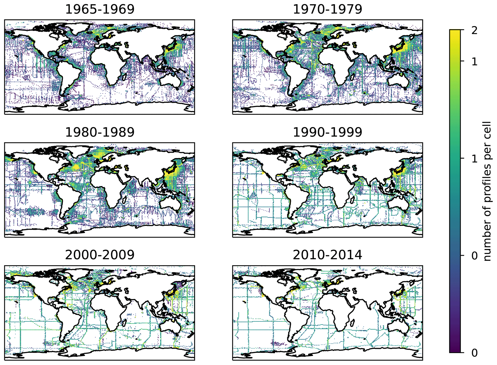
Figure 2 Number of OSD and CTD oxygen profiles aggregated into 1^∘ × 1^∘ longitude–latitude grid cells for 4 decades, from 1965 to 2014. The color scale indicates the number of measurements in log scale.

2 Methods

2.1 Observational data source

We make use of observations from the bottle and conductivity–temperature–depth instruments' (CTD) O₂ data in WOD18. Dissolved oxygen is the third most frequently measured chemical tracer in the ocean, following temperature and salinity. There are approximately 2.8 million temperature, 2.4 million salinity, and 0.9 million O₂ vertical profiles in the ocean station data (OSD or simply bottle data) reported in WOD18. In addition, CTD data include approximately 1 million temperature and salinity profiles, and 0.2 million O₂ profiles. The OSD (i.e., bottle) O₂ data are largely located on the margins of the ocean basins and along repeat hydrographic transects (Fig. 2). O₂ observations in the OSD profile were typically measured by means of a modified Winkler titration method with a precision of about 1 µmol kg⁻¹ (Carpenter, 1965). Most modern oxygen chemical titration measurements are based on Carpenter's whole-bottle titration method and an amperometric or photometric end detection with a precision of about 0.5–1 µmol kg⁻¹ (or approximately, 0.3 %). The CTD O₂ data are based on electrochemical and optical sensors mounted on the CTD rosette samplers, which are periodically calibrated to the Winkler O₂ (Grégoire et al., 2021). The coverage of CTD measurements increased after the 1990s, and that of profiling floats has rapidly increased in recent years. However, the overall spatio-temporal coverage of O₂ observations from bottle and CTD has decreased since the 1990s. Profiling-float O₂ data have increased significantly in the past 10 years; however, the precision is on the order of 1 %–2 % (∼ 2 µmol kg⁻¹), and the data quality control and calibration are still under development, especially in the upper-ocean oxycline (Bittig et al., 2018; Maurer et al., 2021). Float O₂ data have been excluded in this study but will be an important data source, especially after 2010s for the future studies.

2.2 Data pre-processing and optimal interpolation

The pre-processing of the data includes a check for acceptable data quality using the WOD18 quality control (QC) flags. The original WOD18 standard-depth profiles with 102 depth levels are placed into bins which are the 1^∘ × 1^∘ longitude–latitude grid cells with 102 vertical depth levels referenced to the standard depths of WOD18. Of the 102 vertical depth levels, 47 levels are in the upper 1000 m.

The target analysis period is after 1965 when the modern oxygen titration method was established by Carpenter, as referenced above. Some of the data from most recent years are not included in the ESMs, as discussed below, so the analysis ends in 2014. The spatially binned quality-controlled data were averaged at a monthly resolution where mean, variance, and sample size are recorded from 1965 to 2014 for the bottle data and from 1987 to 2014 for the CTD O₂ data. Next, the monthly mean climatology is determined by calculating the climatological monthly mean combining the bottle and CTD O₂ data and then filling data gaps. We are interested in long-term O₂ changes which can be calculated as the anomalies from the monthly climatological mean. Departures from the monthly climatology are recorded as O₂ anomalies for each bin. The binned data are very sparse at a monthly timescale (Fig. 1). For each year, the monthly anomaly data are averaged into yearly anomalies, neglecting the months with missing data. This step increases spatial data coverage significantly while averaging out high-frequency variability in the data, including changes shorter than the yearly timescale, such as waves and eddies. In addition, a 5-year moving window (pentadal) averaging is applied to the yearly anomaly, neglecting the years with missing data. This further increases the spatial data coverage while averaging out variability on the timescale shorter than 5 years. The resulting, pentadal O₂ anomaly data cover the 46-year period from 1967 to 2012.

A relatively simple optimal interpolation (OI) is applied to the pentadal O₂ anomaly data for each year to yield the spatially interpolated O₂ anomalies following Wunsch (1996). This method provides the least-square estimate of the O₂ field on regularly spaced grid cells, minimizing the mean square error of the mapped data for given observations with a covariance function. Stationary and isotropic Gaussian covariance is assumed throughout this study, with the e-folding length scale (L_ref) of 1000 km. This particular choice of length scale controls how far an observation can influence the far field together with the assumed noise-to-signal ratio (ε) of 0.2. The Gaussian assumption may be qualitatively reasonable, but the ocean circulation is neither spatially stationary nor uniform. The use of the Gaussian function allows us to avoid calculating and storing the large and complex covariance structure, but it can distort the resulting maps (Fukumori et al., 1991), which is a caveat for this study. A basin mask is used to interpolate data points only within the same ocean basin such as the Atlantic, Pacific, Indian, and Southern oceans. Each 1^∘ × 1^∘ grid point is assigned to one of the 53 basins defined in Appendix 1 of Garcia et al. (2019). The binned oxygen vector, X, is expressed as a (N × 1) vector, where N is the number of binned data for a particular basin. The objective map of oxygen climatology, Y, is a (M × 1) vector, where M is the number of grid cells for the basin. The optimal interpolation is applied to each basin as follows:

$$\begin{array}{}\text{(1)}& \mathit{Y}=\mathbf{D}{\mathit{E}}^{-\mathrm{1}}\mathit{X},\end{array}$$

where X is the pentadal oxygen anomaly input from the discrete data, and Y is the objective map of (gap-filled) oxygen anomalies. D is a (M×N) data–grid covariance matrix based on the Gaussian function, where $D_{\text{mn}}=\exp (-L_{\text{mn}}^{\mathrm{2}}/L_{\text{ref}}^{\mathrm{2}}$ and L_mn is the distance between the two points. C follows the same definition but for the N×N data–data covariance, and $\mathit{E}=\mathit{C}+\mathit{\epsilon }\mathit{I}$, where ε is the noise-to-signal covariance ratio. For the Southern Ocean, all data points southward of 30^∘ S are used. An example of this process in the year 1991 is shown in Fig. 1. Basin-wise application of optimal interpolation is performed for the O₂ anomalies, resulting in yearly (running pentadal) maps for the 46-year period. The O₂ anomaly field and its standard error field are recorded.

2.3 Ocean deoxygenation trend

Using the yearly maps of the O₂ anomaly field, global and basin-wise O₂ contents are calculated as the volume integral over the upper 1000 m, O(t), where t is time since 1967. The magnitude is referenced to the mean value of the first 10 years, where the 10-year (1967–1976) mean O₂ contents are subtracted from respective O₂ content time series for comparison purposes. Ocean deoxygenation trends are estimated as the slope (a) of the O₂ content time series using standard linear regression:

$$\begin{array}{}\text{(2)}& {\displaystyle }a={\displaystyle \frac{{\mathit{\sigma }}_{\mathrm{t}O}}{{\mathit{\sigma }}_{\text{tt}}}},\text{(3)}& {\displaystyle }b=\stackrel{\mathrm{‾}}{O}-a\stackrel{\mathrm{‾}}{t},\end{array}$$

where σ_tO is the covariance between time and O₂, and σ_tt is the variance in time. (a,b) are the slope and intercept of linear regression. Assuming that the regression errors are normally distributed, the standard error for the slope (ϵ_a) and intercept (ϵ_b) can be calculated as follows:

$$\begin{array}{}\text{(4)}& {\displaystyle }{\mathit{ϵ}}_a=\sqrt{\mathrm{MSE}\left({\displaystyle \frac{\mathrm{1}}{\sum {\left(t_n-\stackrel{\mathrm{‾}}{t}\right)}^{\mathrm{2}}}}\right)},\text{(5)}& {\displaystyle }{\mathit{ϵ}}_b=\sqrt{\mathrm{MSE}\left({\displaystyle \frac{\mathrm{1}}{N_{\text{eff}}}}+{\displaystyle \frac{{\stackrel{\mathrm{‾}}{t}}^{\mathrm{2}}}{\sum {\left(t_n-\stackrel{\mathrm{‾}}{t}\right)}^{\mathrm{2}}}}\right),}\end{array}$$

where MSE stands for the mean square error of regression, t_n is time at nth data point. The gridded O₂ dataset is constructed based on a 5-year running mean. An effective sample size (N_eff) is calculated assuming that 5-year data are independent, thus N_eff ∼ 9 for 46 years of data. These parameters are later used to evaluate the uncertainty and will be used for the comparison between models and observation.

2.4 CMIP6 Earth system models

Two sets of time-varying O₂ fields are derived from the ESMs, including the full field and the reconstructions from the sub-sampled model output (Table 1). We selected a subset of Earth system models participating in the Coupled Model Intercomparison Project Phase 6 (CMIP6), and the outputs for their historical simulation are downloaded from the Earth System Grid Federation (https://esgf.llnl.gov, last access: March 2023). The monthly mean O₂ output is first re-gridded onto the global 1^∘ × 1^∘ longitude–latitude grid for the period of 1965 to 2014. A bilinear interpolation is first performed for the horizontal interpolation, followed by the linear interpolation on the vertical axis to the standard depths of the WOD18. Sub-sampled model output is then generated from the full field where the model output fields were resampled using the same spatial and temporal locations as with the observations. The sub-sampling strategy assumes that a grid box is sampled if, at least, one observation exists within the grid cell at a particular year or month. If so, we retain model data in the sub-sampled dataset. In reality, there could be multiple casts within the same grid and the same year or month, but multiple samples and/or variability within a single cell are not considered. There are slight differences in the land–ocean masks between models, and we use the model topography as they are provided. Similarly to the observational analysis, the sub-sampled monthly O₂ climatology is assembled from the sub-sampled data with the optimal interpolation filling the data gaps using Eq. (1). Then O₂ anomalies are calculated by subtracting the sub-sampled monthly climatology, and they are first aggregated into annual O₂ anomalies, neglecting months without data, followed by the running pentadal averaging. Finally, the basin-wise optimal interpolation is applied to yield the reconstructed O₂ anomaly fields using Eq. (2). These procedures are repeated for each of the models in Table 1. For the comparison purposes, the 5-year moving window averaging is applied to the full field.

Table 1 List of CMIP6 models used in this study. Variants represent decadal-scale variability ensemble members and are coded according to (r) realization, (i) initialization, (p) physics, and (f) forcing. The first available variant, typically noted as r1i1p1f1, is taken from each model.

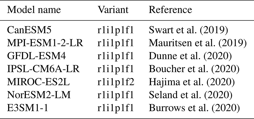
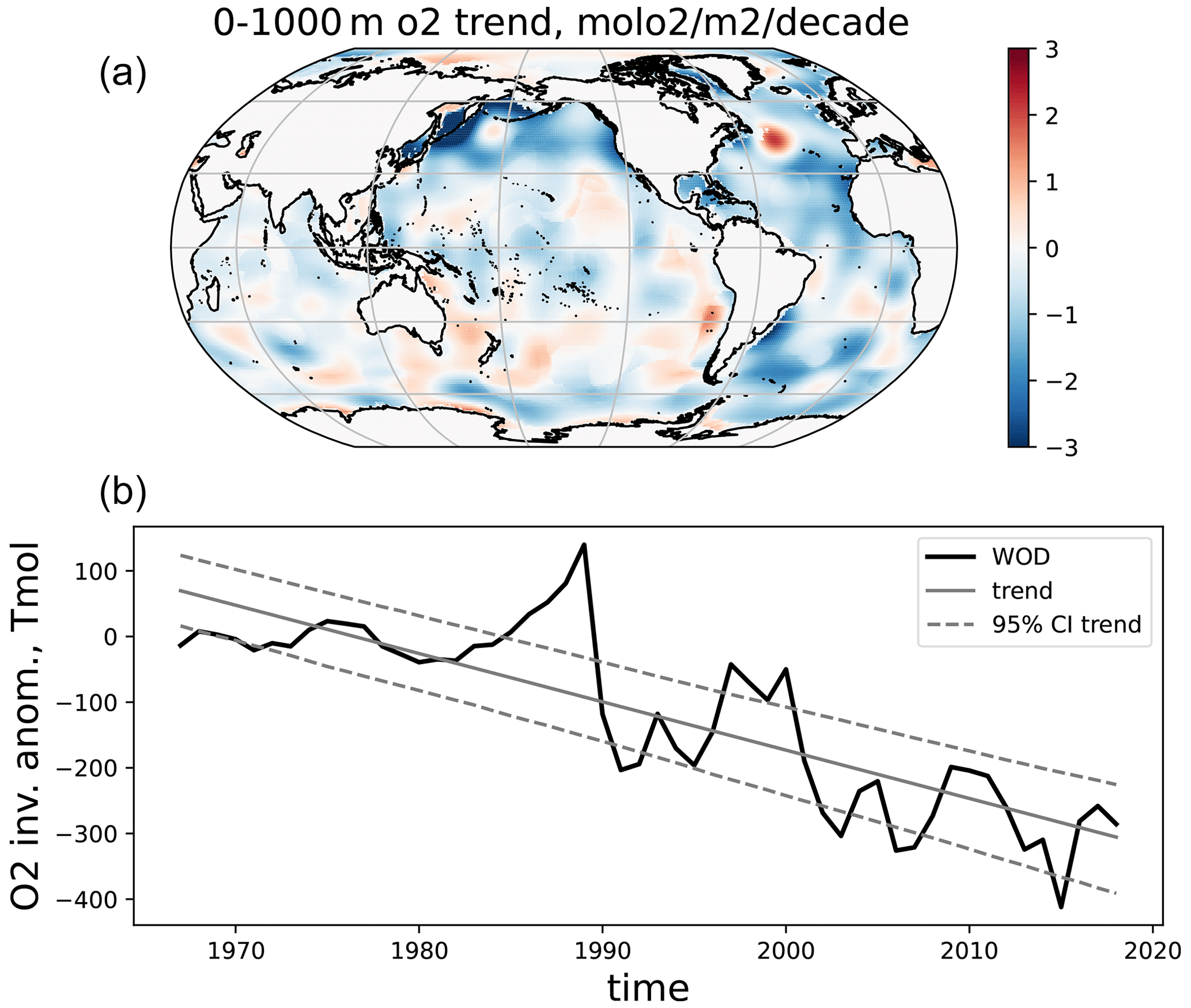
Figure 3 (a) Linear trend of upper-ocean (0–1000 m) column O₂ inventory from 1967 to 2012 from the optimally interpolated pentadal O₂ anomaly based on the World Ocean Database 2018. (b) Time series of oxygen inventory is plotted for the global domain from 0 to 1000 m depth, including its linear trend and the 95 % confidence interval of the trend line. The confidence interval is calculated using a Monte Carlo method.

3 Results

3.1 Observed and modeled O₂ trend maps

The observational trend is first determined based on the optimally interpolated gap-filled WOD18 profiles. The vertically integrated O₂ inventory (0–1000 m) trend pattern is shown in Fig. 3a. While regional differences exist, the basin-scale patterns of the observed O₂ loss are similar to those in previous studies (Helm et al., 2011; Schmidtko et al., 2017; Ito et al., 2017). In the North Atlantic, overall O₂ decline is observed, except for the south of Greenland in the subpolar North Atlantic, where a patch of an increasing trend exists. In the North Pacific, a strong decrease is found in the western subpolar region, spreading from the sea of Okhotsk (Nakanowatari et al., 2007), which may be connected to the reduced ventilation in this region. A weak increase is found in the subtropical North Pacific (Ito et al., 2019), which is related to the multi-decadal natural variability of the North Pacific climate. Oxygen increases are observed in the subtropical Southern Hemisphere oceans and to the south of Greenland. In terms of the global inventory trends, the data suggest a global linear trend of −175 ± 24 Tmol O₂ decade⁻¹ or approximately 1.5 % loss over the 50-year period.

Table 2 From left to right column: spatial pattern correlation (Pearson's correlation coefficients) between observed and modeled upper-ocean (0–1000 m) column O₂ trend and the global trend magnitudes, the pattern correlation between observed modeled O₂ trend patterns (full and sub-sampled optimally interpolated model outputs).

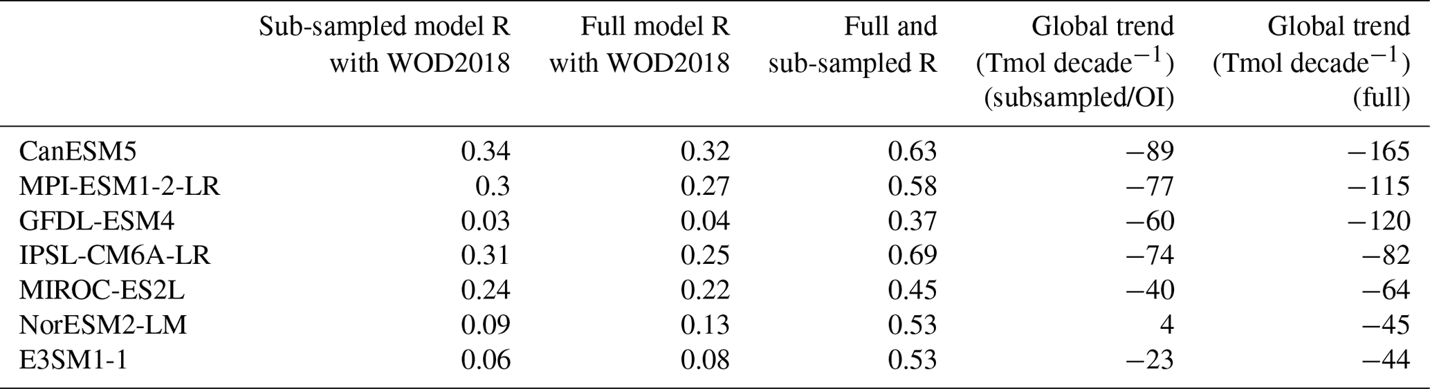
Figures 5 and 6 show the comparison of the trend pattern between the models listed in Table 1 for the full model field (Fig. 5) and the reconstructed model output (Fig. 6). The modeled O₂ trend patterns are moderately correlated to the observations for some of the CMIP6 models, as summarized in Table 2. CanESM5, MPI-ESM1-2-LR, IPSL-CM6A, and MIROC-ES2L exhibit a moderately positive correlation of approximately r=0.3. It is interesting to contrast this result to the hindcast simulation of the earlier generation of ocean biogeochemistry models reported by Stramma et al. (2012). The subset of CMIP6 models in this study is slightly better correlated to observational estimates than the hindcast runs using an earlier generation of models. This is likely due to the improved biogeochemical model structure and parameterization rather than the physical climate forcing. Hindcast simulations are forced by the observed atmospheric variability through the meteorological reanalysis products. In contrast, historical simulations of the CMIP6 models generate natural climate variability that, in general, does not reproduce the phasing of observed variability.

The reconstructed CMIP6 model output is slightly better correlated to the observation than the full model output for the majority (five out of seven) of models, perhaps reflecting the common sampling pattern and gap-filling approach. Comparing the reconstructed and the full field from the same model, the pattern correlation of the O₂ trend ranges from 0.37 to 0.69. While it is not perfect, the OI can estimate the general pattern of the full field with moderate correlation for the 1^∘ × 1^∘ gridded trend maps. This motivates us to further investigate to what extent OI can estimate the O₂ trend for a larger-scale hemispheric and/or global domain.

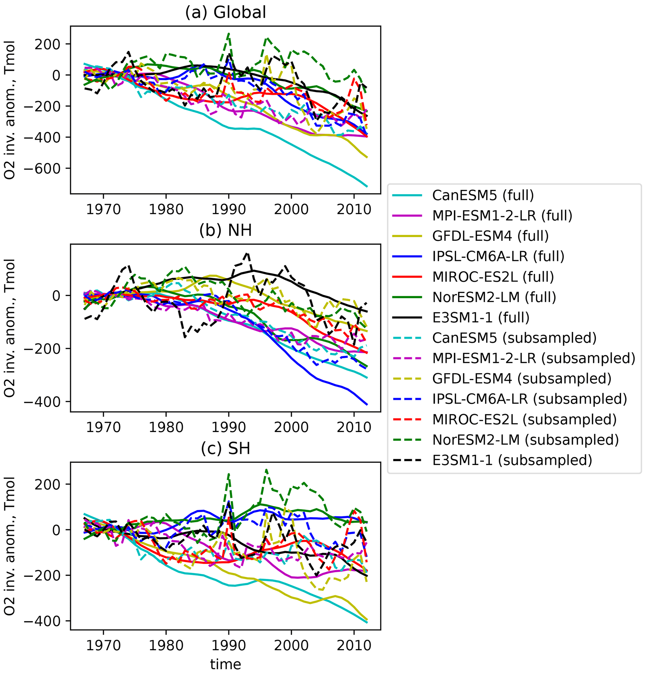
Figure 4 Time series of upper-ocean (0–1000 m) column O₂ inventory from CMIP6 models from (solid line) full model output and (dash line) sub-sampled and optimally interpolated model output. Panel (a) is the global, and panels (b) and (c) are the Northern and Southern hemispheres. The range of the vertical axis for the hemispheric inventories is smaller than the global inventory. The inventory anomaly is referenced in relation to the first 10-year averages.

3.2 Global and hemispheric O₂ inventory time series

The globally integrated O₂ content has a stronger declining trend than in ESMs, and the weak trend bias in models becomes even greater when reconstructed from sub-sampled data (Fig. 4, Table 2). Only one of the models exceeded the observed global trend in the full field (CanESM5, −165 Tmol decade⁻¹; Table 2). When there are no observations nearby, the OI reverts to the background climatology, thus decreasing the amplitude of anomalies. Thus, the estimated O₂ content tends to underestimate O₂ anomalies in the region of sparse sampling. The magnitude of underestimation depends on the distance from observations, which sets the covariance according to the assumed Gaussian function. Figure 4 further shows that the sub-sampling introduces three decadal-scale peaks in the years 1988, 2000, and 2011 for both observations and some of the models (Fig. 4). These quasi-decadal peaks are not apparent in the full model output. We hypothesize that these quasi-decadal peaks are likely spurious, caused by the sparse sampling pattern. The magnitudes of these apparent spurious peaks are on the order of 100 Tmol O₂. To provide a context, they are comparable to the anomalous O₂ inventory increase caused by the eruption of Mt. Pinatubo and subsequent ocean cooling and enhanced ocean O₂ uptake (Fay et al., 2023).

The global inventory time series is divided into the northern and southern hemispheric components (Fig. 4b and c). Comparing the hemispheric and global inventory time series indicates some notable issues with the sub-sampling. First, northern hemispheric trends in some of the full model outputs (IPSL-CM6A-LR and CanESM5) have similar magnitudes to the observational trends. In some other ESMs, the overall magnitudes of the southern hemispheric trends are similar to the observations (GFDL-ESM4 and CanESM5). Overall, the hemispheric trends demonstrate similar magnitudes between the north and the south for observations and models. The reconstructed model outputs appear to underestimate the magnitude of the trends for all models. The magnitude and the causes of this underestimation are of great interest and will be investigated further in the following sections.

Secondly, the observed quasi-decadal peaks primarily appear in the southern hemispheric inventory (Fig. 4e and f, solid black line), and some of the models reproduce these peaks (GFDL-ESM4, MIROC-ES2L, NorESM-LM2, E3SM1-1) for the reconstructed model output (Fig. 4f). There are no apparent peaks in the full model output, confirming that these features are spurious.

Thirdly, in the Northern Hemisphere (Fig. 4c and d), there is a moderate increase towards the late 1980s, and then it decreases strongly during the 1990s. Two of the Earth system models (GFDL-ESM4 and E3SM1-1) show similar increases in the early period (Fig. 4c); however, they underestimate the decreasing trend after the 1990s. These features are distorted in the reconstructed model output. It is difficult to determine whether the apparent increase in oxygen content is meaningful during the 1980s, but similar features are found in earlier studies focusing on the near-surface waters (Garcia et al., 2005).

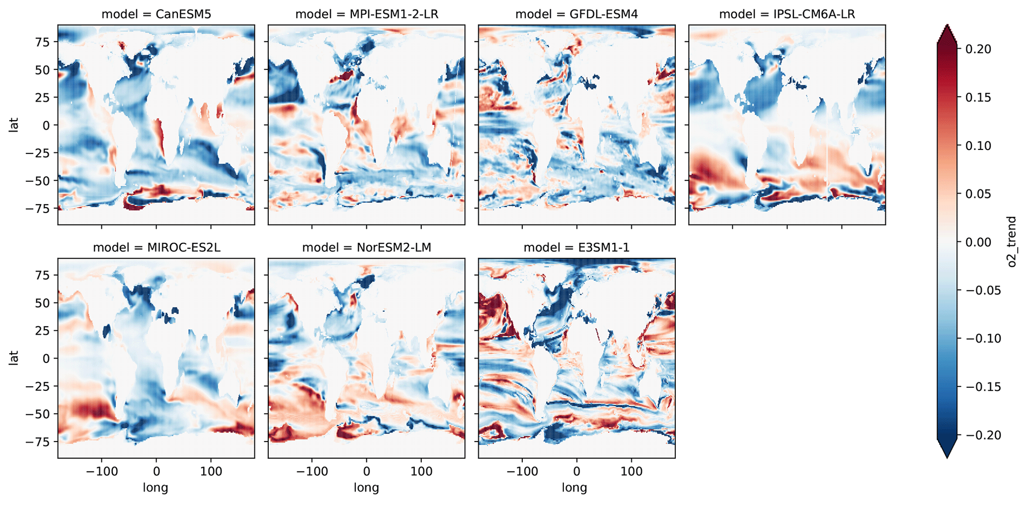
Figure 5 Modeled linear trend of the column O₂ inventory (0–1000 m) from 1967 to 2014 from the full model output.

The models and observations tend to disagree more significantly in the Southern Hemisphere. Modeled inventory trends disagree substantially from one another because of the spurious quasi-decadal noises. While some models exceed the observed magnitude of oxygen decline (GFDL-ESM4, CanESM5), some other models even show increases in the southern hemispheric O₂ inventory (NorESM2-LM, IPSL-CM6A-LR).

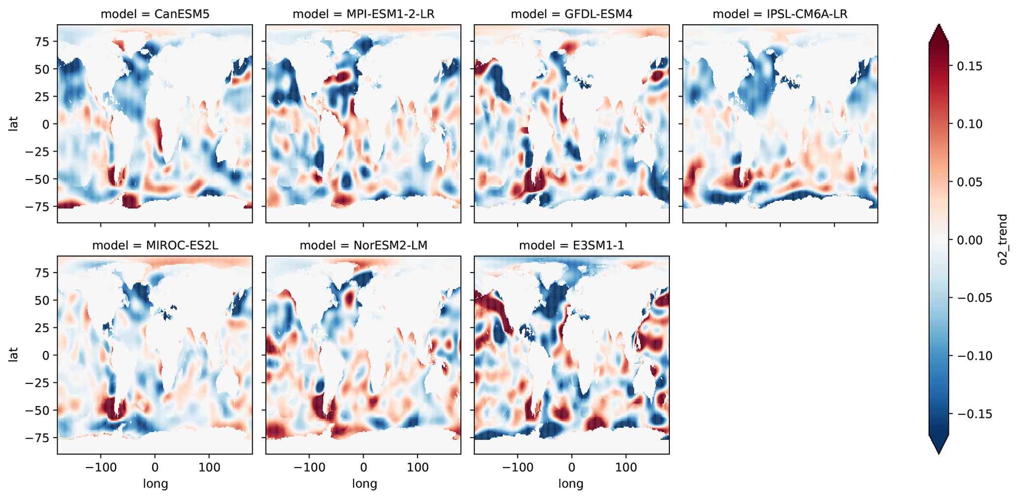
Figure 6 Same as Fig. 5 but for the trend reconstructed from optimal interpolation of sub-sampled model outputs.

3.3 Spatial pattern of O₂ trends and basin-wise inventories

To examine O₂ trends across ocean basins, we divided the global data into 13 regions according to a basin mask (shown in Fig. S1 in the Supplement). The basin O₂ inventories are integrated for each region from the full model output and sub-sampled model (Fig. S2 and S3). Figure 5 shows the spatial patterns of the column O₂ trend (0–1000 m) from the full model output. Blue shading shows strong O₂ loss, and red indicates O₂ increase. The patterns of O₂ trends from the reconstructed model output are displayed in Fig. 6. The effect of sub-sampling does not change the spatial pattern; it only affects the trend magnitudes. As expected, the reconstructed model outputs exhibit weaker trend magnitudes. For each region, the inventory time series are displayed in separate figures from Figs. S4 through S16. For the basin-scale deoxygenation trend, the North Atlantic Ocean is the only basin where all models show the same sign of change relative to the observation for the full-field and reconstructed model outputs (Figs. S2 and S3).

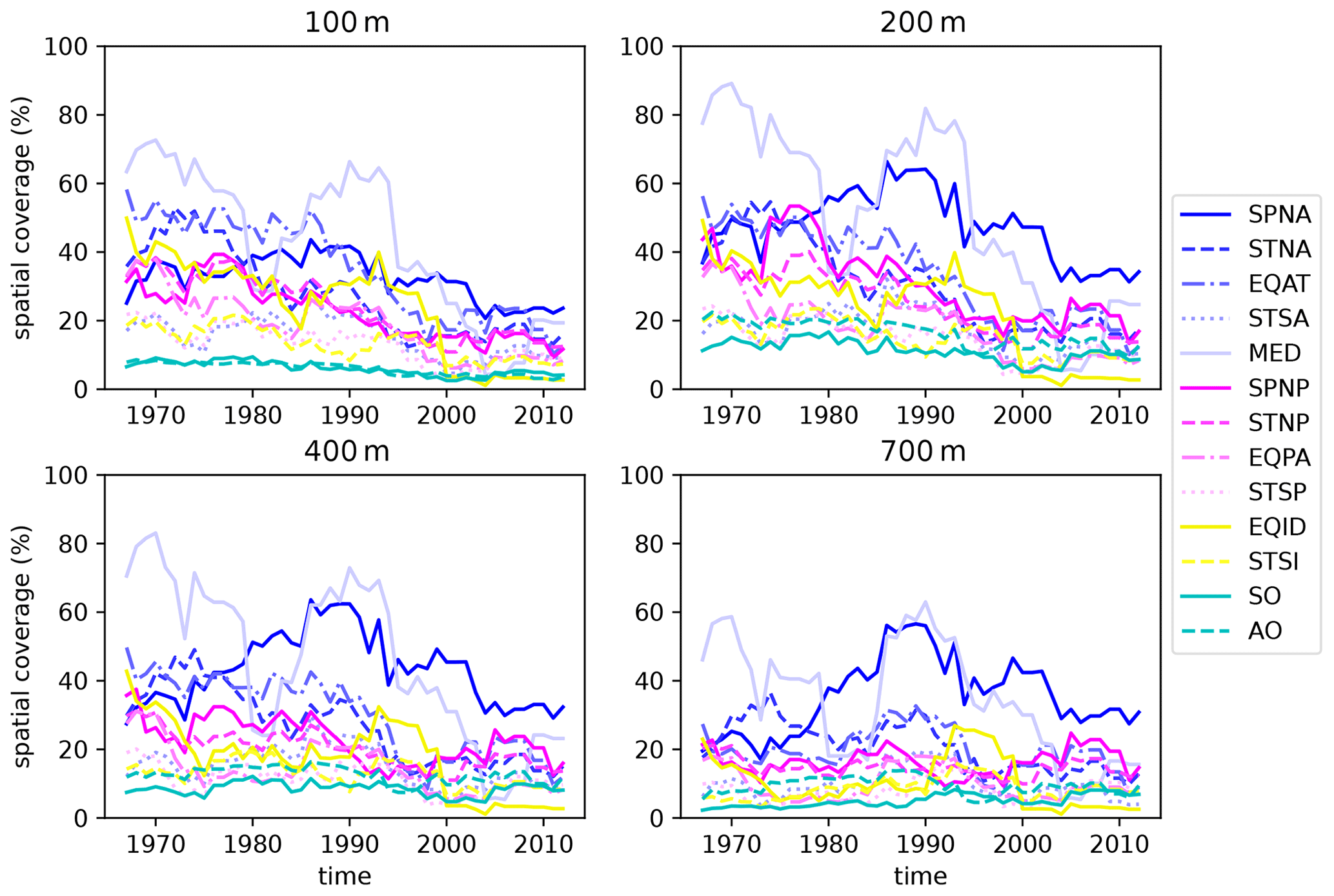
Figure 7 Spatial data coverage of the pentadal O₂ anomaly data from WOD18. The area covered by grid cells with at least one profile is divided by the total area for each basin. Blue lines are Atlantic basins. Magenta lines indicate Pacific basins. Indian basins are in yellow, and cyan is used for the Southern Ocean and the Arctic Ocean. Basin masks are defined in Fig. S1 and are coded by color. Abbreviations for the basin names are as follows: subpolar North Atlantic (SPNA), subtropical North Atlantic (STNA), equatorial Atlantic (EQAT), subtropical South Atlantic (STSA), Mediterranean Sea (MED), subpolar North Pacific (SPNP), subtropical North Pacific (STNP), equatorial Pacific (EQPA), subtropical South Pacific (STSP), equatorial Indian Ocean (EQID), subtropical South Indian Ocean (STSI), Southern Ocean (SO), and Arctic Ocean (AO).

Figure 7 shows the evolution of the spatial data coverage for each basin. To calculate the percent coverage value, the area of grid cells with at least one shipboard profile is divided by the total area of grid cells in each basin. Overall, the North Atlantic and Mediterranean Ocean are the most well observed among the 13 regions. Near-surface waters are better sampled than the deeper layers (400, 700 m). The data coverage evolves over time, depending on the basin. During the 1970s and 80s, there was greater data coverage for near-surface waters (100–200 m), and the near-surface data coverage gradually decreased after the 1980s. However, this pattern is not uniform through the depths. For some regions such as the subpolar North Atlantic, there appears to be no significant decrease in the deeper profile (700 m).

There are several notable features from this comparison. First, models exhibit varying patterns of O₂ changes, and the model disagreements are more pronounced in the Southern Hemisphere oceans, even in the full model output. This is consistent with the varying hemispheric-scale trend magnitude, as shown in Fig. 4e and f. Approximately half of the models show increasing or decreasing trends in the subtropical South Pacific. The observed O₂ decline is strong in the observations, but its time series is noisy, and the discrepancies between the full-field and the reconstructed model output are large in the Southern Ocean (Fig. S17). This is consistent with the persistently low data coverage in the Southern Ocean (Fig. 7). The Southern Ocean contributes significantly to the spurious quasi-decadal peaks that are visible in the hemispheric and global time series (Fig. 4); thus, the observed trend in the Southern Ocean may include large uncertainty.

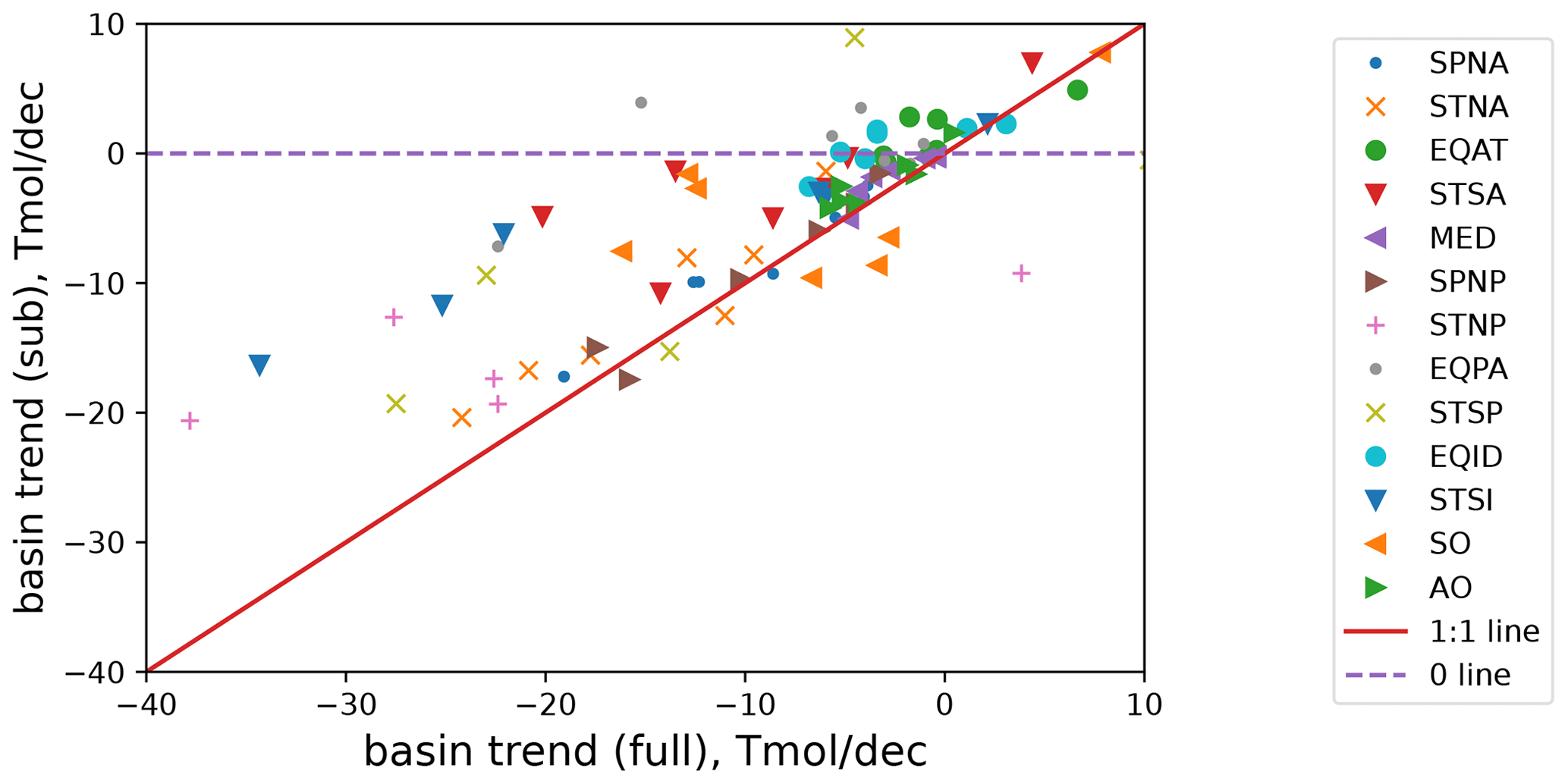
Figure 8 Basin-wise relationship between fully sampled and sub-sampled O₂ trends for seven CMIP6 models. Data points on or near the 1:1 line (solid red) indicate that sub-sampled data adequately reproduced the fully sampled modeled trend. Abbreviations for the basin names are as follows: subpolar North Atlantic (SPNA), subtropical North Atlantic (STNA), equatorial Atlantic (EQAT), subtropical South Atlantic (STSA), Mediterranean Sea (MED), subpolar North Pacific (SPNP), subtropical North Pacific (STNP), equatorial Pacific (EQPA), subtropical South Pacific (STSP), equatorial Indian Ocean (EQID), subtropical South Indian Ocean (STSI), Southern Ocean (SO), and Arctic Ocean (AO).

There are two regions, namely the subpolar and subtropical North Atlantic, where observations and all models agree in terms of the sign of changes. These two regions' inventory time series are displayed in Figs. S4 and S5. In the subpolar North Atlantic, the magnitude of modeled O₂ changes brackets the observation, whereas some models (CanESM5, IPSL-CM6A-LR, E3SM1-1) exhibit even stronger O₂ loss than observations. In the subtropical North Atlantic, these three models exhibit a similar magnitude of O₂ loss as the observations. In the equatorial Atlantic, there is a clear difference between the models and observation. The observation shows a decreasing trend, and not a single model was able to reproduce it. Similarly, the models were not able to reproduce the magnitude of O₂ loss in the subpolar North Pacific, with the exception of MPI-ESM-1-2-LR.

3.4 Synthesis

The basin-wise O₂ trend is compared between the full-field and reconstructed model output in Fig. 8, assessing the ability of the OI method to reproduce the full-field data. In Fig. 8, the horizontal axis is the full model, and the vertical axis is the reconstructed model output. Each dot indicates simulated O₂ trend magnitude for a basin. The solid red line is the 1:1 ratio, indicating where the OI method was able to fully reproduce the trend magnitude. Most of the dots are located between the solid red line and the dashed purple line, indicating that the magnitude of the ocean deoxygenation trend is underestimated due to the OI method applied to sparsely sampled data.

Four regions (subtropical North Atlantic, subpolar North Atlantic, Mediterranean, subpolar North Pacific) performed very well in terms of capturing more than 80 % of the deoxygenation trend in the context of the simulation. These regions are relatively well sampled, and the loss of the trend magnitude due to the OI is minimal. In contrast, the four regions (equatorial Atlantic, equatorial Pacific, equatorial Indian, Southern Ocean) performed very poorly, capturing less than 30 % of the simulated deoxygenation trend. These regions unfortunately are not well represented by the sub-sampled and gap-filled data, showing the limitation of the OI method. The strong negative trend in the Southern Ocean (upper-left panel in Fig. 5) may be highly uncertain, and this is concerning since the Southern Ocean significantly contributes to the global oxygen content. Other basins (subtropical South Atlantic, subtropical North Pacific, subtropical South Pacific, subtropical Indian Ocean, Arctic Ocean) are moderately represented (30 %–80 % of the true trend).

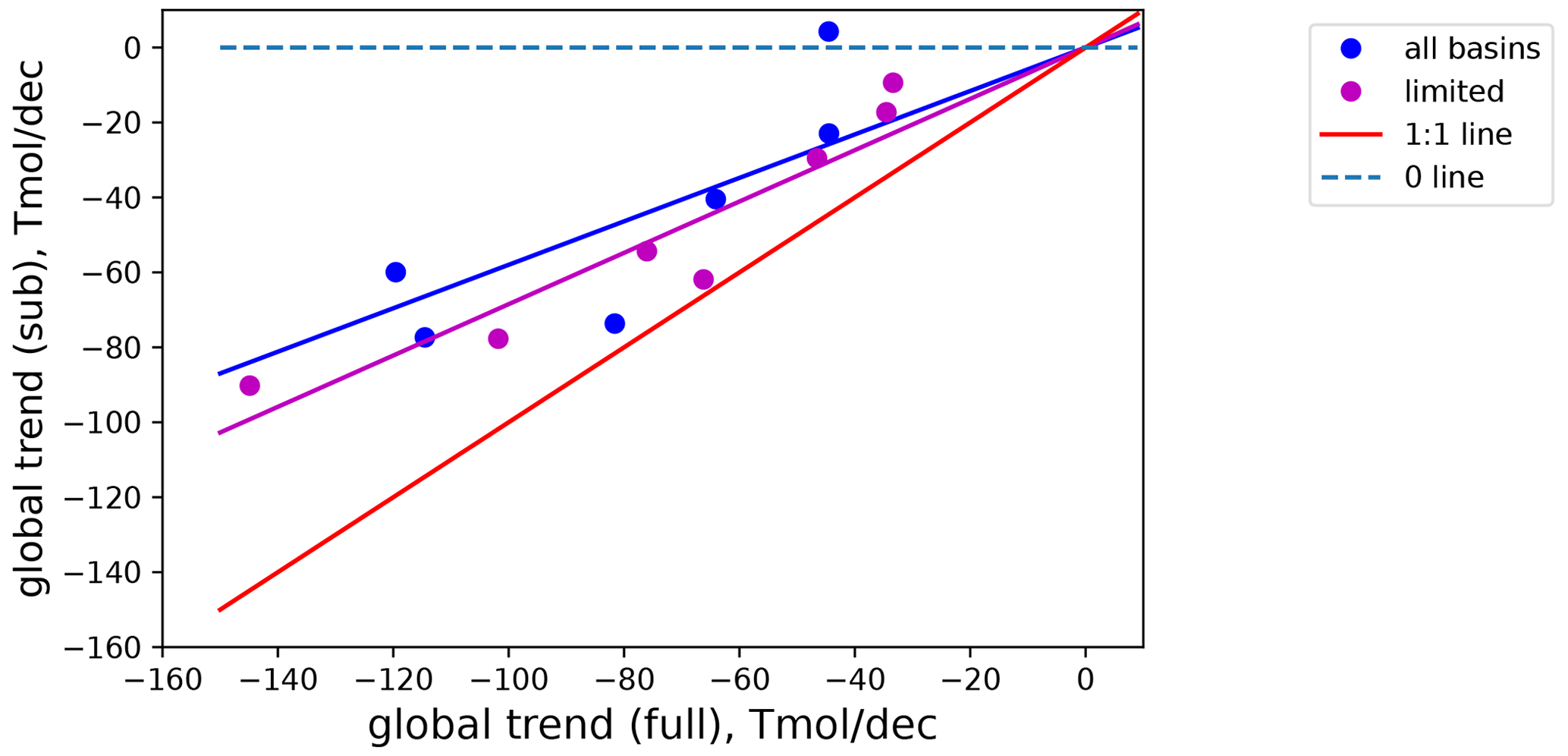
Figure 9 Global relationship between fully sampled and sub-sampled model O₂ trend. Blue dots indicate the seven CMIP6 models with full global model output. Purple dots indicate the same, except the four poorly represented regions (equatorial Atlantic, equatorial Pacific, equatorial Indian, Southern Ocean) are excluded.

To what extent did the OI method underestimate the global deoxygenation trend? Figure 9 illustrates the relationship between the true global trend (on the x axis) and the estimated trend from the sub-sampled model outputs. Each dot comes from a model from two different ways of aggregating the global trend. The blue dots include all basins regardless of the ability of the OI method to reconstruct the true trend. The purple dots exclude the equatorial basins, as well as the Southern Ocean. The linear regression among the seven models informs us that the sub-sampling and the gap filling with the OI method can capture approximately two-thirds (68 %, purple line) of the true trend, excluding the low-confidence regions. Looking at the distribution among the models, the spread of this ratio is 19 %, as calculated by the standard deviation. If all basins are included, the fraction that is retrieved by the OI method decreases to 58 % (blue line).

One of the implications from the model analysis is that the optimal interpolation method used in this study may result in the significant underestimation of the dissolved oxygen trend in observations. The observation-based global oxygen content trend can be adjusted assuming that the ratio of the deoxygenation trend between the sub-sampled and full model output is approximately two-thirds (68 ± 19 %), as determined by the CMIP6 ESMs. Optimal interpolation of the WOD18 oxygen profiles estimated a 1.5 % O₂ decline over the last 50 years, but the true O₂ decline may be in the range of 1.7 % to 3.1 %. This partially overlaps with the recent estimates of the global oxygen decline, which is in the range of 0.5 %–3.3 % (IPCC, 2022), but suggests that the low end of that range is very unlikely.

4 Discussion

The premise of this study is that Earth system models can provide useful information about the uncertainties in the global ocean deoxygenation rate due to the sparse sampling and the specific gap-filling method used with observations. The models disagree amongst each other and with the observations because of different and imperfect representations of processes due to model structures, parameterizations, and the presence of natural variability. However, a model can estimate the observational sampling bias by comparing its true model state to one that is reconstructed by sub-sampling the model output according to the pattern of shipboard profiles (bottle and CTD) from the WOD18.

The model-based analyses in this study are generally consistent in showing that sub-sampling with the gap-filling method yields weaker trends than the full model output. The gap-filling method used in this study is a relatively simple implementation of optimal interpolation (OI), which provides the best-fit distribution of O₂ anomaly in the least-square sense assuming a Gaussian covariance structure of the data. Our mapping approach is admittedly simple, but this choice has certain benefits, for example, that the results from a simple method are easy to understand and that it is also easy to notice and to correct mistakes. It can be replicated by other groups relatively easily. If the ocean deoxygenation has a wide-spread, large-scale signal, as well as regional hotspots, we anticipate that a simple method should, at least, capture the majority of the large-scale components and some regional features. There are some drawbacks in that it tends to smooth out spatial gradients, and it may not represent regional signals very well in data-poor regions. This OI method essentially predicts a diminishing anomaly when there is no observation nearby with the assumed e-folding length scale. If there is a widespread O₂ decrease, the OI can underestimate the trend in a sparsely sampled region. Our result confirmed this tendency for the global deoxygenation trends from the subset of CMIP6 Earth system models. Our analysis, based on seven such models, suggests that approximately two-thirds of the true trend are captured by the reconstructed model output. This conclusion generally applies to all models independently of the model skills in capturing the observed trend for the global and hemispheric inventories (compare left and right column of Fig. 4) and for the basin-wise trends (compare Figs. 5 and 6). Some ocean regions have better coverage than others, and significant regional variations exist for the sampling density and thus the performance of OI. For example, the North Atlantic and subpolar North Pacific are relatively well sampled, and the OI was able to capture more than 80 % of the true trend. In these well-sampled regions, detailed analyses of ocean deoxygenation rates are likely to be fruitful using models and observations using the OI method.

Broadly speaking, the Northern Hemisphere oceans are generally better sampled than the Southern Hemisphere oceans, but the overall trends appear to be equally contributed by both hemispheres (Fig. 4). Basin-wise analysis revealed diverging basin-wise trend patterns among the models (Figs. 5 and 6). There is no consistent pattern in the contributions from different regions to the overall trend regardless of the sampling density. Also, there is no consistent pattern in the sign of multi-decadal O₂ trends, except for the North Atlantic Ocean, where all models are in general agreement. This region has the highest sampling density (Fig. 7), and the full-field and reconstructed O₂ trends are in good agreement (Fig. 8). Data coverage is not the only factor, but it plays an important role in the performance of the OI method. The North Atlantic is sampled at 20 %–50 % density based on 1^∘ × 1^∘ grid cells with decreasing coverage from the surface to deeper depths and from subpolar to subtropical latitudes (Figs. 7 and S17). In the low-sample region, namely, the Southern Ocean, whose data coverage is persistently less than 13 %, the OI method struggled to reconstruct the full-field O₂ trends. In this region, historical observations are limited to certain longitudes or latitudes (e.g., Drake Passage) and the repeat hydrographic cruises (Fig. 2), and it was clearly inadequate to represent the full-field data.

It is useful to compare oxygen content trends using multiple gap-filling approaches to assess the uncertainties from different methodologies (IPCC, 2022). The framework developed in this study may be helpful to further deepen such intercomparison studies and to quantify the skill of different gap-filling methods in the context of model output. Such comparison studies may reveal what sampling density is sufficient to reconstruct the real trend. For such an exercise, it is important to select model-derived oxygen fields that include realistic background variability. For the OI method, it is also crucial to have the covariance structure of the O₂ field. An important caveat for this study is that the models used here were not eddy resolving, and we also used a Gaussian covariance with a prescribed length scale. Mesoscale ocean eddies are energetic features with characteristic spatial scales of 10–100 km and characteristic timescales of several months. The model outputs did not include this type of internal ocean variability, and the modeled fields did not include the mesoscale noises that are present in the observation. The use of non-eddying models reduces the level of internal ocean variability to be much lower than the observations. Thus, we are not able to address to what extent the trend estimates vary depending on the presence of ocean eddies and smaller-scale variability, which is a caveat in this study. It may be possible to emulate the mesoscale eddy noise (and uncertainties from other factors such as instrumental errors) and to estimate a more realistic covariance structure of O₂ fields using outputs from detrended high-resolution simulations, but this is beyond the scope of this paper and is left for future study.

This paper has focused on mapping and the trends of total O₂, which consist of two sub-components, oxygen saturation (O_2sat) and apparent oxygen utilization (AOU). O_2sat strongly depends on temperature, with a minor contribution from salinity, and explains less than half of the observed O₂ trend (Ito et al., 2017; Schmidtko et al., 2017). Most uncertainty is associated with the AOU component since temperature is measured with much higher sampling rates, and its mapping uncertainty would be significantly lower than that of O₂ or AOU. This paper has also focused on the mapping in depth coordinates. While it is beyond the scope of this paper, interpolating O₂ along isopycnal surfaces may potentially reduce the mapping uncertainty. Temperature variation on an isopycnal is much smaller than that of O₂ so the O_2sat variation would be better constrained along isopycnals. Also, ocean transport in the interior ocean is primarily oriented along isopycnals, and the interpolation on isopycnal surfaces can potentially reduce the spurious errors. However, there could be technical difficulties as the bottle O₂ measurements come from discrete bottle samples, and the sampling depths are unlikely to match the location of desired isopycnals, leading to an interpolation error. In the end, one would have to try and evaluate how much uncertainty can be reduced by mapping along density horizons, which would be a promising topic for future study.

While sampling sparseness is likely a major source of uncertainty, there are other sources of uncertainties that remain open for further investigation. Historical O₂ profiles may have evolving precision and uncertainty that are difficult to replicate in a model-based study. For example, a Winkler titration performed on a Nansen bottle during the 1960s may have different precision than a more recent Winkler titration done on a Niskin bottle using amperometric or photometric end-point detection methods. Looking ahead, integration of autonomous float O₂ data will pose challenges in terms of assessing uncertainties that are changing with the evolution of measurement techniques. Another important area of future investigation would be the uncertainties from natural variability. A recent modeling study (Fay et al., 2023) showed overlapping magnitudes of externally forced and internally generated O₂ anomalies in the context of volcanic eruption. Quantification of natural variability is difficult to achieve using observations or a collection of single runs from multiple models. The best approach would be to use multi-model large ensembles with adequate ensemble members of randomized natural climate variability.