Temporary stratification promotes large greenhouse gas emissions in a shallow eutrophic lake

Shallow lakes and ponds undergo frequent temporary thermal stratification. How this affects greenhouse gas (GHG) emissions is moot, with both increased and reduced GHG emissions hypothesised. Here, weekly estimations of GHG emissions, over the growing season from May to September, were combined with temperature and oxygen profiles of an 11 ha temperate shallow lake to investigate how thermal stratification shapes GHG emissions. There were three main stratification periods with profound anoxia occurring in the bottom waters upon isolation from the atmosphere. Average diffusive emissions of methane (CH₄) and nitrous oxide (N₂O) were larger and more variable in the stratified phase, whereas carbon dioxide (CO₂) was on average lower, though these differences were not statistically significant. In contrast, there was a significant order of magnitude increase in CH₄ ebullition in the stratified phase. Furthermore, at the end of the period of stratification, there was a large efflux of CH₄ and CO₂ as the lake mixed. Two relatively isolated turnover events were estimated to have released the majority of the CH₄ emitted between May and September. These results demonstrate how stratification patterns can shape GHG emissions and highlight the role of turnover emissions and the need for high-frequency measurements of GHG emissions, which are required to accurately characterise emissions, particularly from temporarily stratifying lakes.

1 Introduction

Freshwaters are key sites for the processing of greenhouse gases (GHGs), methane (CH₄), carbon dioxide (CO₂) and nitrous oxide (N₂O). Shallow lakes, in particular, have been identified as hot spots of CH₄ release, particularly when ebullition is taken into account (Davidson et al., 2018; Aben et al., 2017). The certainty that freshwaters are large emitters of GHGs contrasts with the uncertainties associated with the quantities emitted, and this is in large part due to historical paucity of measurements (Cole, 2013). A recent study has identified the highly variable emissions from lakes and ponds (Rosentreter et al., 2021). Whilst different morphometric features and chlorophyll a explained some of the emission patterns (Deemer and Holgerson, 2021), it is also clear that a dearth of measurement combined with these highly variable emissions makes determining the drivers and controls of those emissions challenging, which in turn makes predicting future emissions difficult.

The current and future effects of climate change on lakes in general and on their GHG emissions are relevant questions as there is potential for positive feedbacks and synergies with other human impacts such as eutrophication (Davidson et al., 2018; Beaulieu et al., 2019; DelSontro et al., 2016; Meerhoff et al., 2022). Taking a broad metabolic theory of ecology approach, temperature increases should promote methanogenesis and shift the balance from primary production to respiration, increasing CO₂ emission at cellular and ecosystem scales (Yvon-Durocher et al., 2010). However, empirical and experimental data indicate that temperature is not the sole controller of primary production and methanogenesis. In particular, eutrophication, and the promotion of large algal crop, has been associated with increased emissions of CH₄ and N₂O (DelSontro et al., 2016) both by diffusion and ebullition (Zhou et al., 2019). Furthermore, in what is globally the most abundant lake type, small shallow lakes, where macrophytes can colonise large areas of the lake bed, trophic states and the dominance of submerged plants or algae may be more important than temperature in shaping GHG dynamics (Davidson et al., 2015, 2018; Bastviken et al., 2023).

Climate change effects on lakes are not limited to increases in average temperatures and lengthening of the growing season. Increases in both the frequency and the intensity of heat waves are predicted, which will promote the warming of surface waters and in turn make permanent and temporary thermal stratification of lakes more likely (Woolway and Merchant, 2019), even in lakes typically classified as non-stratifying (Kirillin and Shatwell, 2016). A recent study by Holgerson et al. (2022) identified stratification and mixing patterns in small water bodies, with permanent summer stratification common and frequent mixing occurring in larger standing-water (> 4 ha) lakes. Such periods of stratification and mixing events are likely to have profound effects on GHG dynamics. Emissions of gases, in particular CH₄, which accumulate in the isolated bottom waters of a stratified lake, occurs upon mixing and can make very significant contributions to cumulative emissions (Schubert et al., 2012). High-resolution studies of sites that undergo temporary stratification are rare, although Søndergaard et al. (2023b) have recently showed how stratification shapes patterns and processes across the entire ecosystem, including short-term effects on dissolved GHG concentrations in bottom and surface waters. In terms of the effects of stratification on GHG dynamics, there are potentially antagonistic processes at work in a stratified lake. On the one hand, the “shield effect” results in lower temperatures at the sediment surface, slowing down metabolic processes that scale with temperature, i.e. methanogenesis and mineralisation of organic carbon (C), reducing emission and promoting C burial. On the other hand, anoxia at the sediment surface may shift processes towards fermentation, increasing the proportion and total amount of CH₄ produced and perhaps reducing C burial (Bartosiewicz et al., 2019). Recent work combining empirical observations and models has suggested that shielding effects are larger than the anoxia effects and that stratification, in general, increases C burial and reduces GHG emissions (Bartosiewicz et al., 2015). The stratification-induced isolation of bottom waters has been reported to lead to reduced ebullition of CH₄ and a shift to diffusive pathways (Bartosiewicz et al., 2015). It might, however, be predicted that in shallow lakes stratification would lead to much larger CH₄ release as anoxic conditions would limit CH₄ oxidation by CH₄-oxidising bacteria (MOBs) (Bastviken et al., 2008). There may also be other factors with the potential to increase GHG emissions, such as sediment organic content and lake trophic status (DelSontro et al., 2016), which may interact with stratification patterns in shaping GHG emissions.

In this study, we used data from a shallow lake with high-frequency measurements of temperature profiles combined with weekly measurements of dissolved gas concentrations in the surface and bottom waters and continuous measurement of ebullitive emissions of CH₄ to track the effects of lake stratification on GHG emissions. The key question was how ebullitive and diffusive fluxes of the key GHGs – CH₄, CO₂ and N₂O – respond to temporary thermal stratification.

2 Materials and methods

2.1 Study site

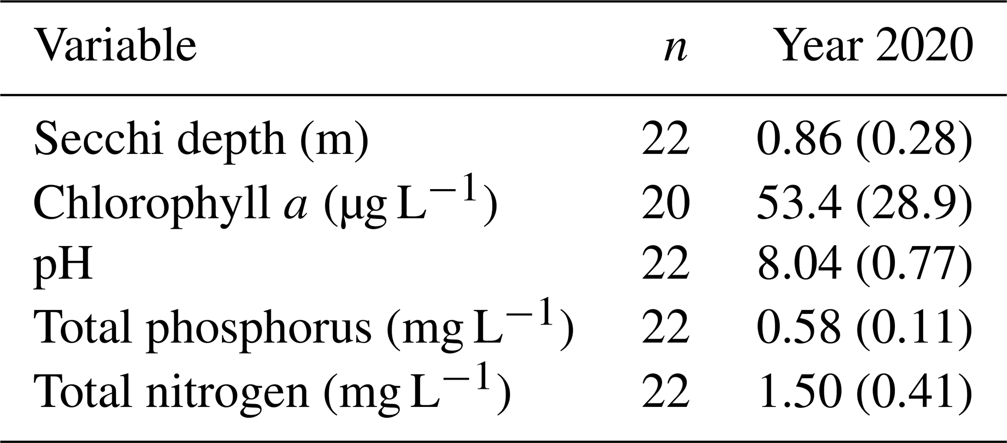
Lake Ormstrup, located in Denmark (lat 56.326^∘, long 9.639^∘) (Fig. 1, depth map with GHG sampling locations), is an 11 ha shallow lake (average depth of 3.4 m), with a maximum depth of 5.5 m and a relatively long hydraulic retention time (> 1 year). The lake is eutrophic with high total phosphorus (TP) and chlorophyll a (Table 1; Søndergaard et al., 2023b) and very sparse occurrences of submerged plants.

Table 1 Summary of lake information, summer mean values and standard deviations of a range of variables.

2.2 Depth profiling and high-frequency measurements

In June 2020, a NexSens (NexSens Technology, Fairborn, OH, USA) CB-450 data buoy system was deployed at the deepest point of the lake equipped with a NexSens TS210 thermistor string with temperature nodes measuring at four levels: one sensor “in air”, ca. 5 cm above the water surface (but shielded from direct light), and three sensors at −1, −2 and −3 m relative to the water surface. In addition, two Aqua TROLL 500 (In-Situ, Fort Collins, CO, USA) multi-sondes were mounted near the surface (−1.0 m) and at a deeper-water depth (−3.8 m). The near-surface and deeper-water sondes were configured with sensors to measure dissolved oxygen (DO) and water temperature (T_w). The optical sensors were calibrated according to the manufacturer's guidelines and checked on a weekly basis.

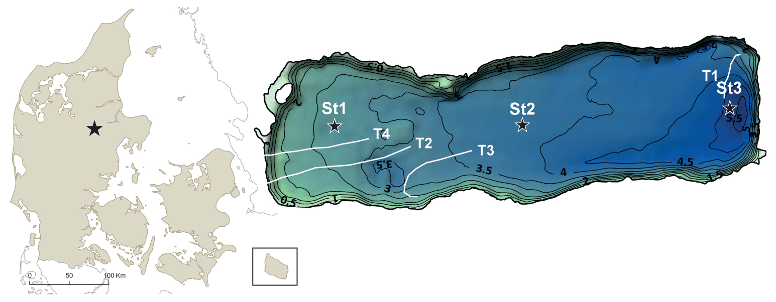
Figure 1 Lake Ormstrup bathymetry and sampling stations for surface- (St1, St2, St3) and bottom-water greenhouse gas sampling (St3). Transects of 10 bubble traps were placed on T1–T4. Adapted from the Søndergaard et al. (2023b).

The optical sensors of the Aqua TROLL 500 have a built-in wiper mechanism to clean sensor heads to hamper bio-fouling. The wiper function was enabled to perform cleaning in sync with sensor measurements, hence every 15 min. In addition, manual cleaning of sensor heads was done every week, whilst routine manual field monitoring was carried out at the lake. Prior to the deployment of the buoy, and as a validation exercise for the buoy data, weekly manual profiles of DO and T_w were collected at the deepest point.

Periods of stratification and the depth of the thermocline were defined using the R package rLakeAnalyzer (Winslow et al., 2019) based on the density gradient of the water column from the weekly manual profiling of the system. During periods defined as stratified, there were partial mixing events where the depth of the thermocline changed, and there was some mixing of the sub-epilimnetic water and the surface waters, whilst the bottom waters below 3.5 m remained undisturbed.

2.3 Water chemistry

Water samples for the analysis of chlorophyll a were collected weekly from 20 April 2020 from surface (−0.5 m) water at station 3 (Fig. 1). A volume of water ranging from 0.2 to 1 L was filtered; the GFC papers were preserved for chlorophyll a analysis, which were determined spectrophotometrically after ethanol extraction (Jespersen and Christoffersen, 1987); and alkalinity was measured weekly by Gran titration (Søndergaard et al., 2005). Depth profiles of temperature, electrical conductivity (EC) and dissolved oxygen (DO) were measured manually with an Aqua TROLL 500 probe from every −0.5 or −1 m down to a −5 m depth).

2.4 Greenhouse gas sampling

2.4.1 Dissolved concentration

Samples of dissolved concentrations of CH₄, CO₂ and N₂O were collected weekly from 20 April 2020 from surface waters and weekly from surface and bottom waters from 26 May to 13 October 2020. The samples were taken using headspace equilibration (McAuliffe, 1971), where 20 mL of water was collected from just below the water surface, and 20 mL of N₂ was introduced as a headspace in a 60 mL syringe and then shaken vigorously for 1 min. The 20 mL headspace was then transferred to a 12 mL pre-evacuated glass vial.

Gas concentrations in the headspace were determined on a dual-inlet Agilent 7890 gas chromatograph (GC) system interfaced with a CTC CombiPAL autosampler (Agilent, Nærum, Denmark) (Petersen et al., 2012). For the GC, certified CO₂, CH₄ and N₂O standards were used for calibration and validation. Aqueous concentrations in N₂O, CH₄ and CO₂ were calculated from the headspace gas concentrations according to Henry's law and using Henry's constant corrected for temperature and salinity (Weiss, 1974; Weiss and Price, 1980; Wiesenburg and Guinasso, 1979). A recent study (Koschorreck et al., 2021) has identified significant bias in the estimate of CO₂ concentrations using headspace equilibration at lower concentrations. We applied Koschorreck et al.'s (2021) correction using separately measured alkalinity.

The fluxes of N₂O, CH₄ and CO₂ between the water and the overlying atmosphere were estimated as

$$\begin{array}{}\text{(1)}& f_{\mathrm{g}}=k_{\mathrm{g}}\left(C_{\mathrm{wat},\mathrm{g}}-C_{\mathrm{eq},\mathrm{g}}\right),\end{array}$$

where f_g is the flux of a specific gas g, k_g is the piston velocity of the gas, and $C_{\mathrm{wat},\mathrm{g}}-C_{\mathrm{eq},\mathrm{g}}$ is the gradient of concentration between the concentration of gas dissolved in the water (C_wat, g) and the concentration of gas the water would have at equilibrium with the atmosphere (C_eq, g).

We calculated a gas transfer velocity k₆₀₀ for each sampling occasion using the relationship based on wind speed described in Cole and Caraco (1998).

$$\begin{array}{}\text{(2)}& k_{\mathrm{600}}=\mathrm{2.07}+\mathrm{0.215}{U}_{\mathrm{10}}^{\mathrm{1.7}}\end{array}$$

U₁₀ is the mean daily wind speed at 10 m (m s⁻¹) obtained from the Danish Meteorological Institute (DMI; 20×20 km grid data).

$$\begin{array}{}\text{(3)}& k_{\mathrm{g}}=k_{\mathrm{600}}{\left({\displaystyle \frac{{\mathit{Sc}}_{\mathrm{g}}}{\mathrm{600}}}\right)}^x\end{array}$$

Sc_g is the Schmidt number (Wanninkhof, 1992) of the specific gas g. We chose $x=-\mathrm{2}/\mathrm{3}$ as this factor is used for smooth liquid surfaces (Deacon, 1981).

Daily flux rates were calculated using linear interpolation of the weekly surface measurements from each of the sampling points. The diffusive surface water fluxes were calculated by taking an average of the daily flux rate from 12 May to 13 October 2020 for each location. Then an average of the three locations was multiplied by the area of the lake and the number of days covered by the study; here 126 d was chosen to match the period over which ebullition was measured.

The total contents of the gases in the lake's bottom waters were calculated from the dissolved concentration of the gases multiplied by an estimate of the volume of the water in the hypolimnion. The volume of water in the hypolimnion was estimated from the lake profiles, which were manually conducted on the day of sampling. The top of the hypolimnion was determined by the depth below which oxygen was less than 0.5 mg L⁻¹. A detailed bathymetry of the lake allows the calculation of the area and therefore the volume of water that lies below a given depth.

During the study period two major turnover events occurred: this process of lake turnover and full mixing, which can take a number of days, and the outgassing process, which can take even longer. The oxygen data from the buoy indicated that it can take up to 4 d, and this provides time for CH₄ oxidation to occur (Søndergaard et al., 2023b). In order to estimate the amount of CH₄ oxidised over the course of the multiple days of degassing, we directly measured CH₄ oxidation rates in the surface waters of the lake. This was done in June 2023 in five locations in this lake using methods outlined in Thottathil et al. (2019), where five water samples from five different locations were used, each incubated over 4 d, and the change in the CH₄ concentration was used to calculate oxidation rates. We applied the minimum (0.267 µg CH₄-C L⁻¹ h⁻¹), mean (0.44 µg CH₄-C L⁻¹ h⁻¹) and maximum (0.58 µg CH₄-C L⁻¹ h⁻¹) oxidation rates to estimate the range of CH₄ oxidation likely to have occurred over the course of the two main turnover events. Assuming that the degassing took 4 d, these rates would consume between 2 % and 8 % of the CH₄ contained in the hypolimnion. Using the mean oxidation value the turnover fluxes were reduced by 4.1 % on 30 June 2020 and by 6 % on 25 August 2020.

2.4.2 Ebullition

The ebullitive flux of CH₄ was estimated using a total of 40 floating chambers placed on 4 transects of 10 chambers each (Fig. 1). The chambers have a volume of 8 L and a surface area of 0.075 m², similar to those used by Bastviken et al. (2015). As the existing literature has indicated that ebullition decreases as water depth increases (Wik et al., 2013), the transects were placed on the shallower slopes of the western end of the lake to maximise the measurement of the low end of the depth gradient (Fig. 1). The average and maximum depths of each transect were as follows: 293 and 472 cm (T1), 181 and 267 cm (T2), 223 and 300 cm (T3), and 166 and 220 cm (T4). The chambers were set on 14 May 2020 and sampled every 2 weeks from this date and on one occasion after 1 week until 17 September, which is a period of 127 d. A total of 20 mL of samples was taken from the floating chamber and injected into a pre-evacuated 12 mL vial (Exetainer, Labco). Gas concentrations were determined on the same GC as described above (Petersen et al., 2012).

The ebullitive flux of CH₄ was estimated as

$$\begin{array}{}\text{(4)}& {\displaystyle \frac{p_{\mathrm{gas}}\times {\mathrm{Vol}}_{\mathrm{bub}}}{t\times A}},\end{array}$$

where p_gas is the concentration of CH₄ in the gas that was trapped, Vol_bub is the volume of the chamber (i.e. 7 L), t is the time during which the samples were collected and A is the area of the chamber (i.e. 0.075 m²).

A portion of the CH₄ released via ebullition in the chamber would have re-dissolved in the water or might have leaked through the chamber walls, thus underestimating the ebullitive flux. We made a number of measurements to constrain this error and to compare estimates based on static chambers with other approaches. The results show that whilst static chambers underestimate ebullition, given the temporal variability of ebullition, static chambers that are continually deployed provide a better estimate of average ebullition than short-term (24–48 h) deployment using portable gas monitors or flushing chambers.

Therefore, whilst the static-chamber method cannot be said to accurately quantify CH₄ emissions, it can be relied upon to compare differences in ebullition between time periods, with the caveat that it always gives an underestimate of the actual ebullitive flux.

Total ebullitive flux from the lake was calculated by taking the mean of the emissions from each transect over the 126 d period, then taking the average of the means of four transects and multiplying this by the time of the deployment of the chambers in days, which was 126 d, and by the area of the lake. This gives a total ebullitive flux of CH₄ for the lake over the period of measurement from May to mid-September.

The three different flux types, surface diffusion, ebullition and turnover emission, were then converted into comparable units of total lake emissions (as grams or kilograms of gas) over the studied period and also CO₂ equivalents using a conversion factor related to their 100-year global warming potential (GWP) of 28 for CH₄ and 265 for N₂O.

2.5 Statistical methods

To test for a significant difference among the emissions from the stratified and mixed phase, we used generalised least squares (GLSs) with a variance function to account for the heterogeneity of variance between the phases. In the case of the ebullitive flux, as the collected phase often covered periods including both mixed and stratified phases, there were three categories, namely mixed, stratified, and both mixed and stratified. All analyses were carried out in R version 4.2.1 (R Development Core Team, 2022), and the GLS used the nlme package (Pinheiro and Bates, 2023).

3 Results

3.1 Lake physical and chemical characteristics

Depth profiles measured weekly from April show that stratification was initiated by 26 May 2020. This may have broken down briefly and may have been established again, visible from the temperature sensors for the buoy on 5 June 2020 (Fig. 2). There was then 12 d of mixing followed by a stable period of stratification with the onset of 14 June 2020 for a duration of 16 d until a mixing event around 30 June 2020. The following 2 weeks had cooler water and a mixed water column and thereafter a ca. 6 d period of stratification from 15 to 21 July 2020. A mixed phase of 2 weeks then followed until stratification was reestablished on 4 August 2020 and persisted until the end of August. Partial mixing is indicated by the buoy data from 21 August 2020, but the weekly manual profile of deeper water indicates that full mixing did not occur until after 25 August 2020. The effects of the stratification and mixing events on the high-frequency DO data measured at −3.8 m are clear, with rapid deoxygenation occurring after the onset of stratification and oxic bottom waters returning when the lake mixed (Fig. 2). The patterns in chlorophyll a also follow, to some degree, those of stratification, with the exception of early spring. Chlorophyll a values were extremely high in spring, peaking at the start of June 2020 and falling gradually (Fig. 2, Søndergaard et al., 2023b). During the periods of stratification, chlorophyll biomass was lower, and when a mixing event occurred the values increased, which is particularly evident in the July mixing periods (Fig. 2).

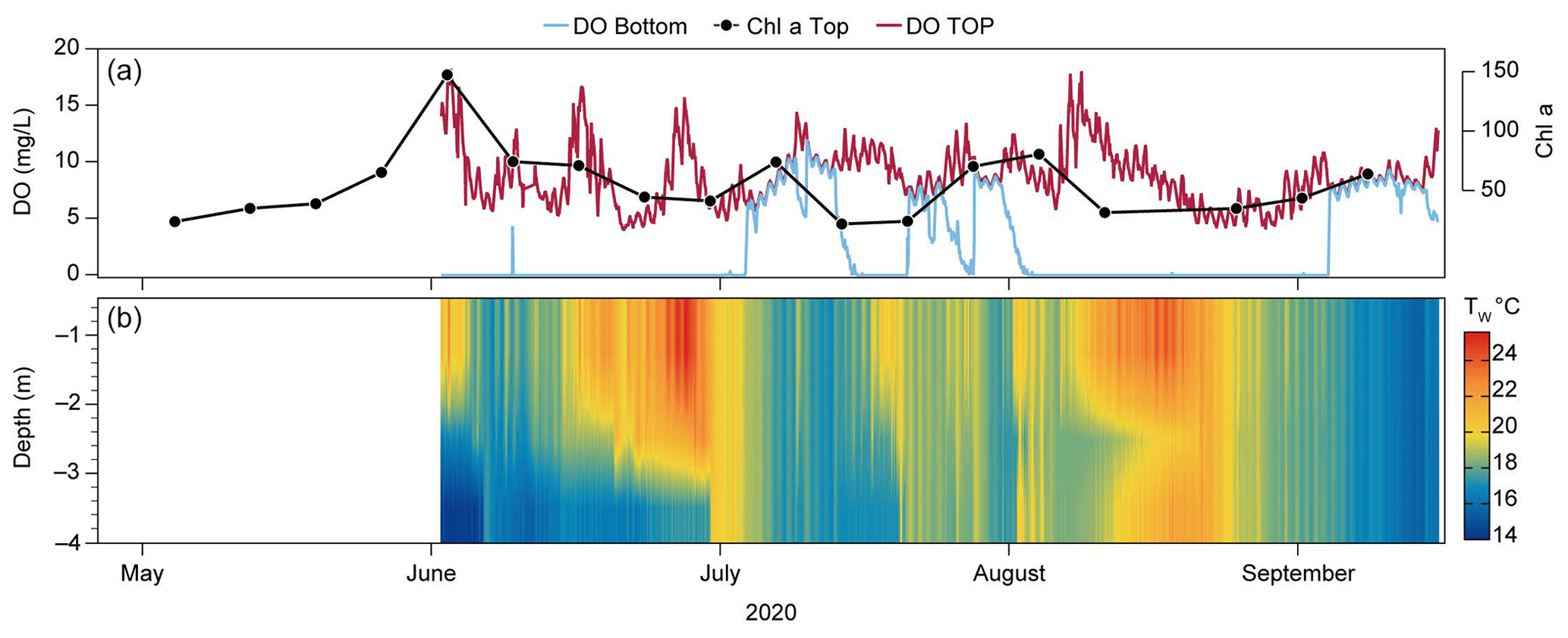
Figure 2 Temperature profile from June 2020 when the buoy was deployed and surface- and bottom-water oxygen from June to the end of September 2020. Manual chlorophyll a (µg L⁻¹) values are also given in the top panel.

3.2 Concentrations of dissolved gases and fluxes from the surface waters

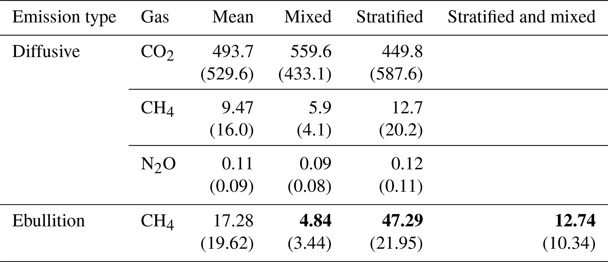
The concentrations of the dissolved gases showed great variation between near- and below-surface atmospheric concentrations in some cases, with up to an extremely high concentration (over 5 mg CH₄ C L⁻¹) in the bottom waters on 30 June 2020. There was some spatial heterogeneity in the surface waters, with the more littoral locations showing the greatest variation and the highest values (Figs. 3, 4, 5). In particular, the most littoral zone, where the water was shallower around 1 m in depth, showed the highest values just prior to, or coincident with, the stratification turnover. Table 2 shows the mean diffusive flux of each gas over the sampling period along with the mean flux in mixed and stratified phases. For CO₂ there was a lot of temporal variation in flux dynamics, though not a large difference between mixed and stratified phases in terms of mean values (Table 2). There were some periods of CO₂ influx in spring and late summer, and these tended to coincide with the end of a mixed phase and the start of the stratification phase. Nitrous oxide concentrations were generally low (Figs. 4 and 5), with the lake being a source of N₂O in the spring period and a sink or a very small source thereafter. The CH₄ concentration in the surface waters (Fig. 3) and the calculated diffusive emissions were relatively low but did increase in the stratification periods with higher average values (Table 2 and Fig. 6). There was also some spatial variation with higher CO₂ and CH₄ diffusive emissions in the shallower sampling locations, both in stratified and mixed conditions (Fig. 6).

Table 2 Mean greenhouse gas flux (CO₂: mg CO₂-C m⁻² d⁻¹, N₂O: mg N₂O-N m⁻² d⁻¹, CH₄ both diffusive and ebullitive in mg CH₄-C m⁻² d⁻¹) from the lake from spring to autumn 2020. The emissions are divided into diffusive and ebullitive emissions. The mean values for all the surface-water stations and all four transects of the chambers are given. The emissions areas, separated into mixed versus stratified phases, and their SDs are also given. Ebullition was collected for a period covering 2 weeks, so on a number of occasions it covered both mixed and stratified periods; thus ebullition has a third category where both mixed and stratified conditions that occurred are given. Ebullition was significantly different across the three phases (signified by bold text); diffusive fluxes were not significantly different for p values of 0.05.

The most significant patterns in the GHG concentration were evident in the bottom waters sampled at −4.5 m, which accumulated to very large concentrations of CO₂ but particularly CH₄ in the periods of stratification (Figs. 3 and 4). The ratio of CO₂ to CH₄ is illustrative in highlighting how stratification has altered the biogeochemical processes in the hypolimnion with CH₄ production becoming more prevalent. For example, on 30 June 2020 after 16 d of stratification, the CO₂ : CH₄ ratio in the bottom waters was 0.8, whereas 7 d later, after the mixing event, it was 187 at the same depth.

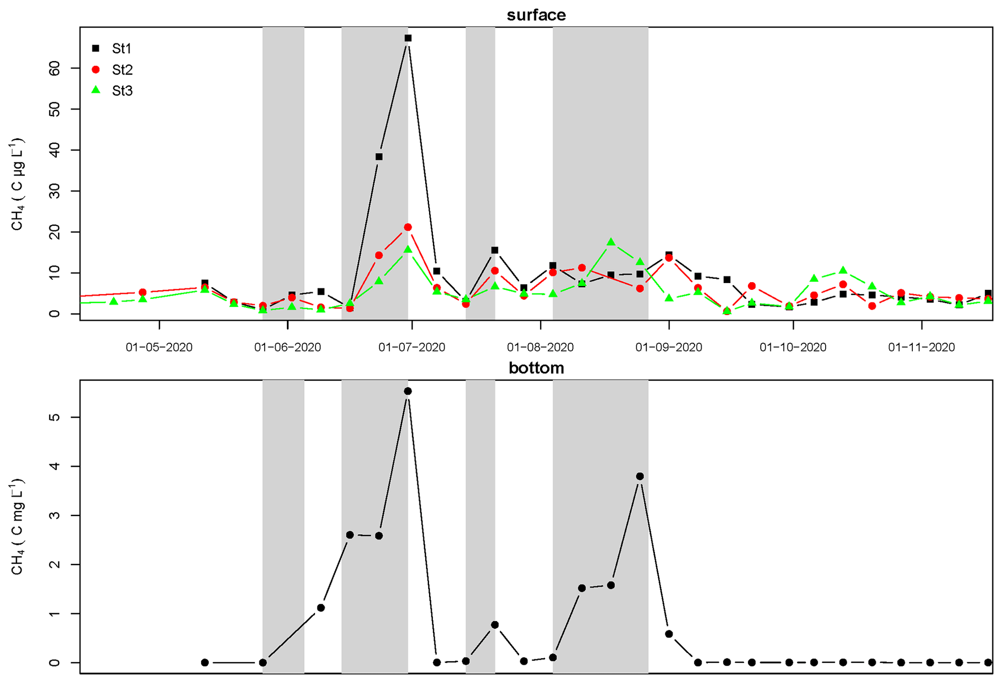
Figure 3 Dissolved CH₄ concentrations from surface and bottom waters. Thermal stratification periods are highlighted in grey, and the white background indicates mixed waters.

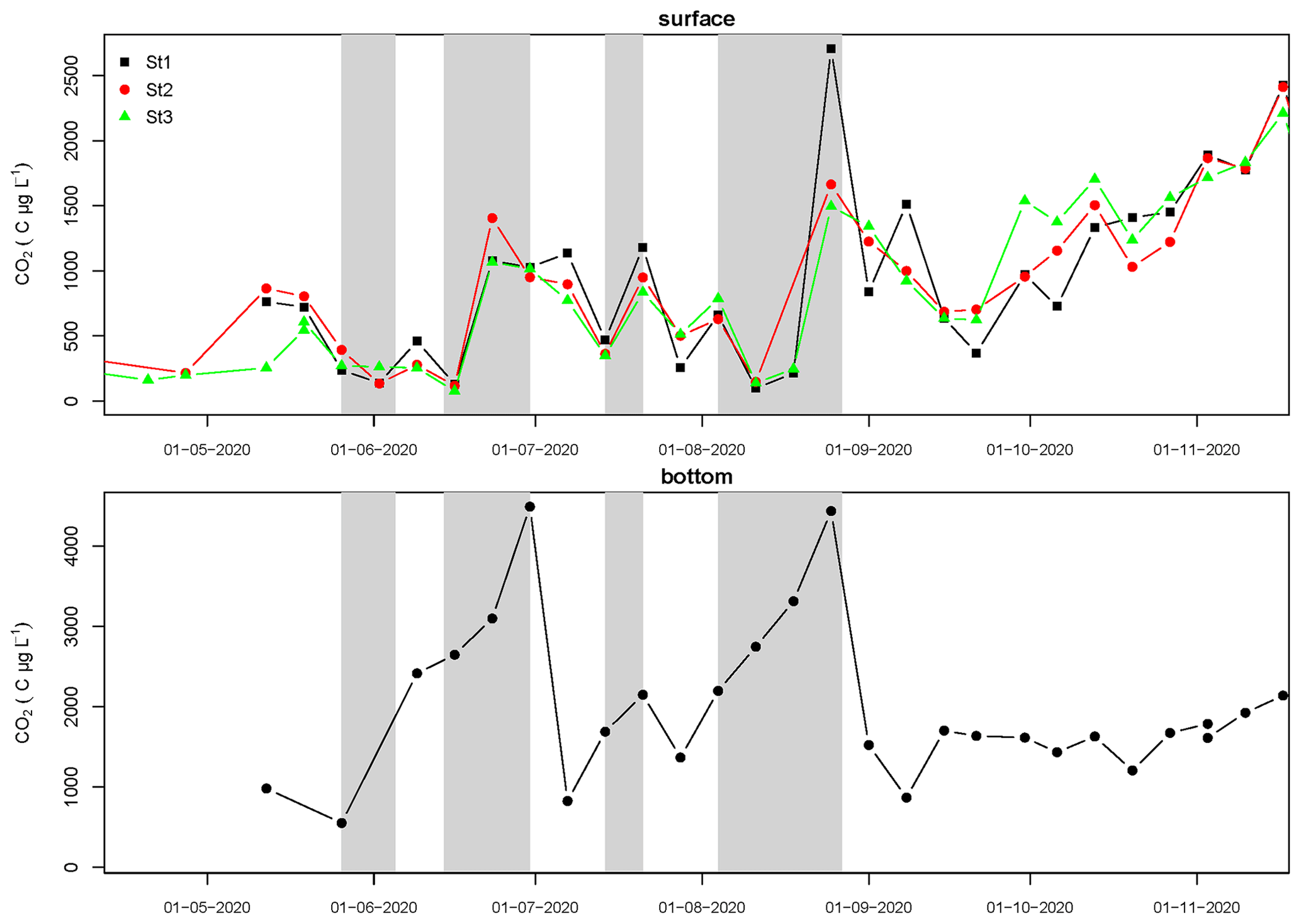
Figure 4 Dissolved CO₂ concentrations from surface and bottom waters. Thermal stratification periods are highlighted in grey, and the white background indicates mixed waters.

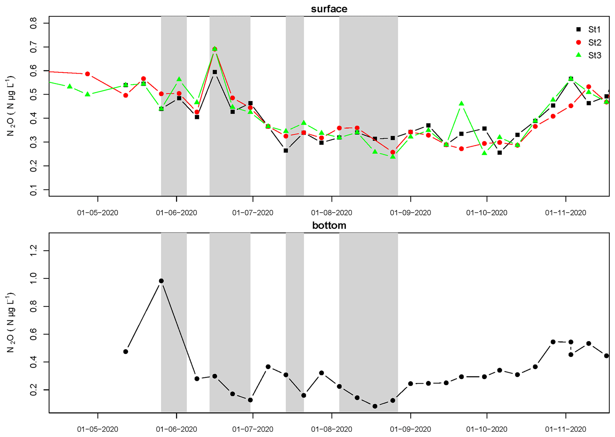
Figure 5 Dissolved N₂O gas concentrations from surface and bottom waters. Thermal stratification periods are highlighted in grey, and the white background indicates mixed waters.

3.3 Ebullitive fluxes

The CH₄ bubble flux, presented here as mean values for each of the four transects, ranged from 0.303 to 81.1 mg CH₄ C m² d⁻¹ for the individual transects over the growing-season measurement. There is a very clear, statistically significant impact of stratification on the ebullitive efflux of CH₄, with stratified periods showing significantly higher levels of emission (Fig. 7 and Table 2). In addition, there was a difference in average emissions among the different transects, with those with a lower average water depth (T2 and T4) having lower emissions than the transects with chambers over deeper water (T1 and T3) (Fig. 7). The samples collected from the chambers reflect 2 weeks of bubble and diffusion collection, and the quantification of the flux is therefore an average of the period of chamber deployment, which was 2 weeks, or in one case a single week (Fig. 7). This 2-week period on occasion covered both stratified and mixed phases, and on these occasions efflux was intermediate between purely mixed and stratified periods (Table 2 and Fig. 7).

3.4 Total lake fluxes

Scaling up the results to total flux of gases from the whole lake over the period of study and including the estimated emissions from two turnover events show a very different effect of stratification on the balance of the types of emissions for the three gases. The majority of CH₄ emissions (56 %) result from the two short-lived turnover events (Fig. 8), whereas their contribution to CO₂ and N₂O emissions was 5 % and 1 %, respectively.

Fluxes of CO₂ and N₂O were mostly diffusive, which represented 95 % of emissions of both gases. The methane diffusive flux was 14 % of the total emission, whereas CH₄ ebullition was more than twice as much at 29 % of the total CH₄ emission. In terms of global warming potential, CO₂ and CH₄ emissions were comparable, but the contribution of the turnover efflux was the dominant factor for CH₄ emissions.

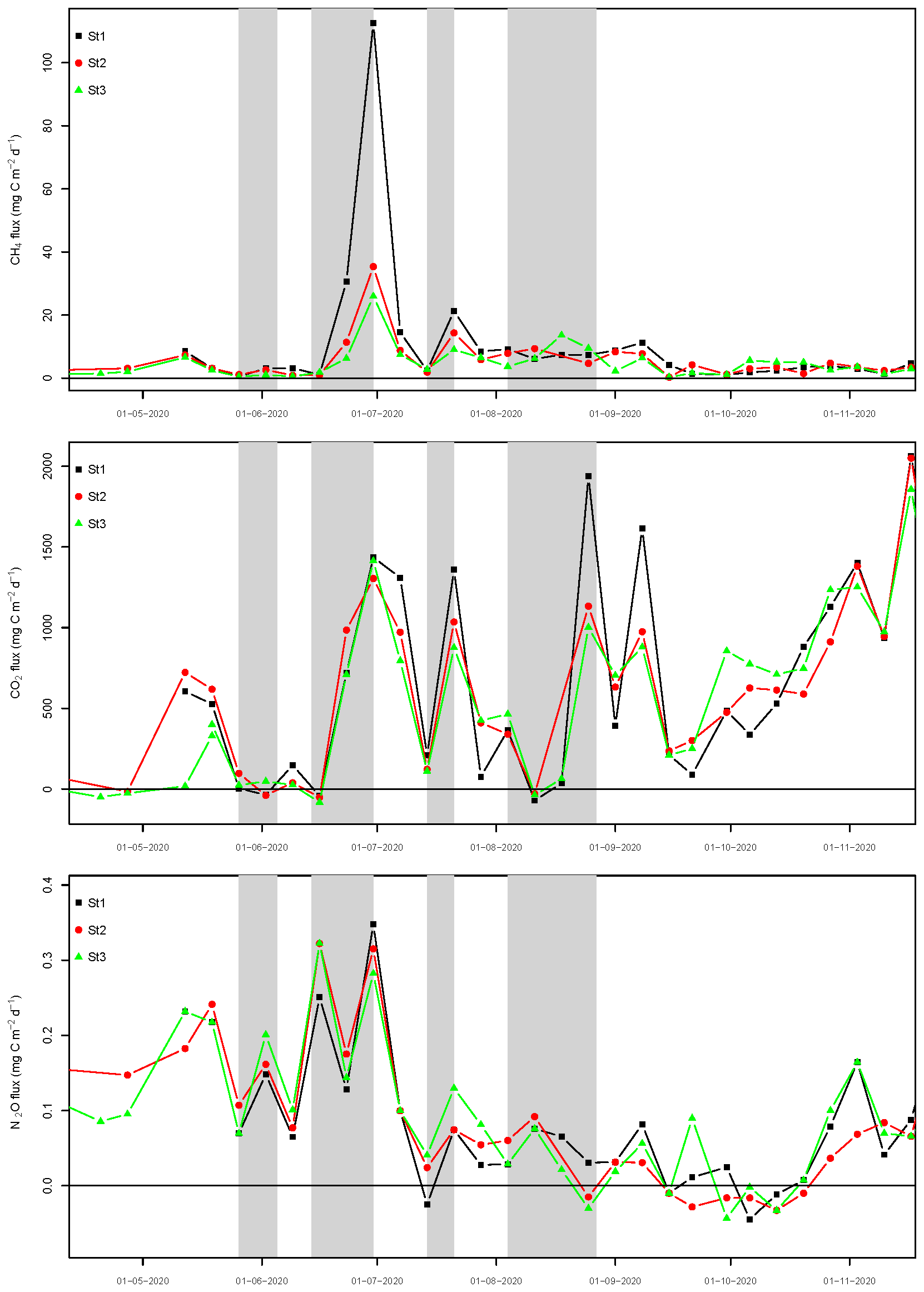
Figure 6 Lake Ormstrup surface fluxes of the CH₄, CO₂ and N₂O gases based on dissolved concentration. Thermal stratification periods are highlighted in grey, and the white background indicates mixed waters.

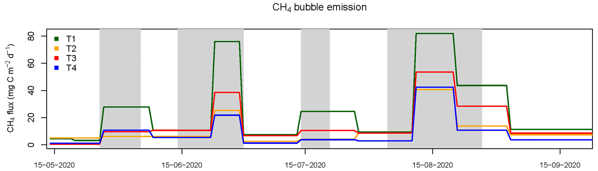
Figure 7 Plot of CH₄ ebullition averaged for each transect (10 chambers per transect). Data were collected from 40 traps every 2 weeks. Thermal stratification periods are highlighted in grey, and the white background indicates mixed waters.

4 Discussion

This study set out to assess the role of thermal stratification in the GHG dynamics in a lake undergoing frequent but temporary stratification. We found that the emission of the three GHGs showed different degrees of variation between the mixed and stratified phases. The largest and most significant variation was in CH₄ ebullition (Table 2), whilst the difference in diffusive fluxes, though marked for CH₄, was not significant. The mean of the total emissions from Ormstrup in the stratified phase (59.9 mg CH₄–C m⁻² d⁻¹) corresponds relatively closely to the mean of the total emissions (ebullition plus diffusion) reported for lakes in this size range (47 mg CH₄–C m⁻² d⁻¹) from a paper synthesising multiple studies (Rosentreter et al., 2021). The mean emissions for the whole period (26.6 CH₄–C m⁻² d⁻¹) were lower than Rosentreter et al.'s (2021) but similar to other studies, with mean emissions of 30.9, 20.7 and 22.7 CH₄–C m⁻² d⁻¹ reported by Peacock et al. (2021), Sø et al. (2023) and Peacock et al. (2019), respectively, whereas the average CO₂ (504 mg CO₂–C m⁻² d) at Ormstrup was lower than the 993.5 mg CO₂–C m⁻² d⁻¹ measured by Peacock et al. (2021) but higher than the 264.6 and 205.1 mg CO₂–C m⁻² d⁻¹ measured by Sø et al. (2023) and Peacock et al. (2019), respectively. The different temporal resolutions and durations of these studies, including 11 single-day sampling from April to December (Peacock et al., 2021), 5 d continuous sampling on one occasion in late September (Sø et al., 2023) and a single early-summer snapshot (Peacock et al., 2019), make direct comparison difficult. The data here do, however, provide a clear answer to the question of how thermal stratification affects GHG dynamics in shallow eutrophic lakes with an increase in total emissions (diffusion, ebullition and turnover) during the stratified period (Table 2, Fig. 9). Previous work, combining observations and modelling, has suggested opposite patterns (Bartosiewicz et al., 2019) as the shielding effect of the stratification results in cooler bottom waters, which reduces CH₄ production due to the process being temperature dependent (Bartosiewicz et al., 2016). This strong shielding effect may apply in deeper lakes experiencing more stable stratification or less eutrophic lakes. The results here from a relatively shallow eutrophic lake indicate that temporary stratification causes increases in GHG emissions.

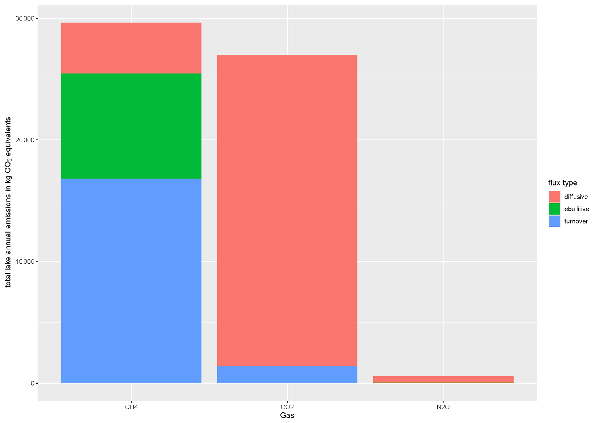
Figure 8 Total lake emissions per gas over the growing season in CO₂ equivalents. The emissions are divided into different emission modes: diffusive, ebullitive and turnover fluxes. All estimates contain some uncertainty; the ebullitive flux in particular is an underestimate, and the turnover flux also contains a great deal of uncertainty.

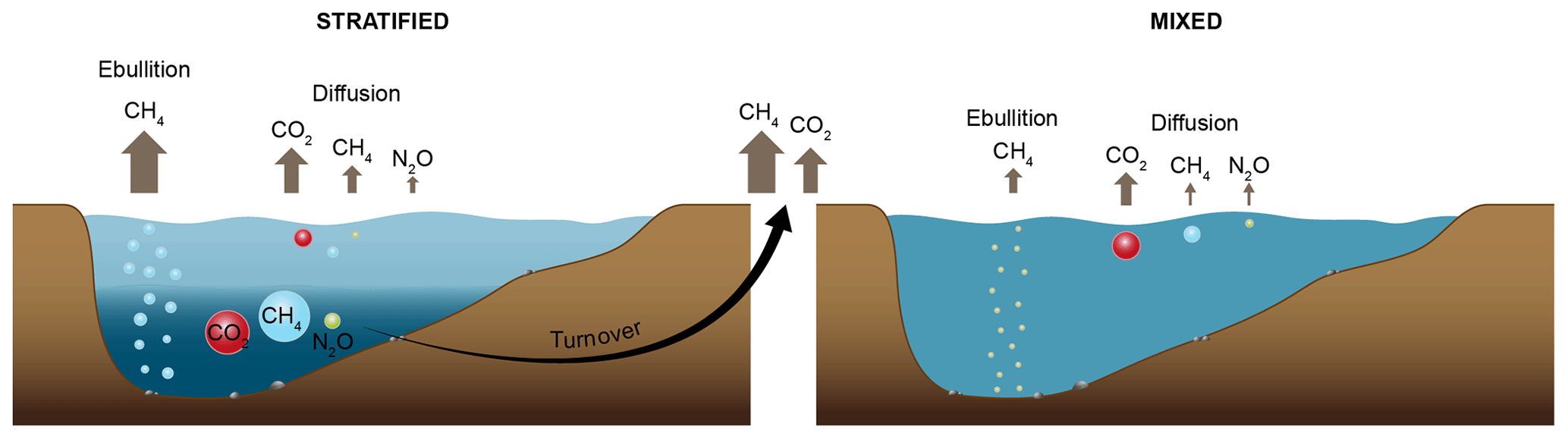
Figure 9 Summary of the quantities of the gases present in the water and the volumes emitted from the different pathways. The size of the arrow is proportional to the emissions from each pathway. The stratified state is on the left, the mixed state is on the right and the turnover flux is in the centre.

4.1 Diffusive fluxes

Diffusive emissions did not, on average, show a strong stratification effect (Table 2). In particular, variation in N₂O emissions did not match patterns of stratification, with emissions more directly related to nitrate concentrations (Audet et al., 2020), as reflected by the fact that the lake is a sink of N₂O in late summer when nitrate was below detection limits for several weeks. There were peaks in emissions of CH₄ and CO₂ at the end of stratification periods, particularly in the shallower-water sampling points (Fig. 6). There were periods of influx of CO₂, which coincided somewhat with periods of stratification, but the pattern was not consistent as other factors, for example, chlorophyll a concentration, also play a role.

Littoral zones can have markedly different GHG dynamics than deeper zones due to shallower water having lower pressure (Wik et al., 2013), less time for CH₄ oxidation (Bastviken et al., 2008) or abundant plants, which influence a range of biogeochemical processes (Davidson et al., 2018; Esposito et al., 2023). It is therefore possible that littoral zone dynamics could cause these differences. However, the increase occurred at all three sampling points at the end of June 2020, which indicates a lakewide driver, and the peak may represent the start of mixing after stratification. Strong winds were measured on 29 and 30 June 2020 (Søndergaard et al., 2023b), coincident with these increased littoral emissions. These winds would have caused lateral movement of the surface water, causing an upwelling of bottom water, rich in CH₄ and CO₂, in the littoral margins at the opposite end of the lake. Thus, whilst we do not have direct evidence, it seems more likely that these increased emissions in the littoral zone were driven, at least in part, by the upwelling of GHG-rich bottom waters.

4.2 Ebullitive fluxes

In contrast to the diffusive flux, the ebullitive emission of CH₄ shows a very clear response to stratification with an order of magnitude difference in emissions between periods where the sampling reflected purely mixed or stratified periods (Table 2 and Fig. 7). The 2-week resolution of the sampling meant that some samples covered both stratified and mixed phases, and these samples had intermediate fluxes, as they covered both low- (mixed) and high-emission (stratified) periods. The spatial variation in ebullition is also illustrative of the impacts of stratification and the role of anoxia in shaping CH₄ fluxes. The two transects with the largest mean and maximum depths (T1 and T3) had the largest emissions, with the deeper of the two (T1) having the highest emissions and showing the largest relative increase during the stratification phases. This pattern is different from that found by some other studies where bubble emissions were larger in shallower water (Wik et al., 2013), although in this and another study (Sø et al., 2023), there was an increase in bubble flux in deeper water in late summer. The deeper water at Ormstrup experienced anoxia early in the season, resulting in locations with deeper water having higher ebullition rates than shallower areas. This is at odds with ideas stemming from the metabolic theory of ecology stating that temperature (Yvon-Durocher et al., 2014), in particular at the sediment surface (Bartosiewicz et al., 2019), can be used to predict CH₄ efflux. Whilst CH₄ production is temperature dependent at the cellular level, CH₄ emissions are rather independent of the sediment temperature; for example, in the first 2 weeks of July 2020 emissions were low, and the sediment surface temperature was relatively high. Thus, temperature alone is a poor predictor of ecosystem-scale CH₄ emissions.

It should be noted that the method used to estimate bubble flux here, where floating chambers are sampled every 2 weeks, is a “less-than-perfect” method, which in nearly all cases will underestimate ebullitive flux. Logistical and financial constraints make continual sampling difficult, and here we balanced these constraints against the greater time required to apply more accurate methods, such as bubble traps (Wik et al., 2013) and automatic-flushing chambers (Bastviken et al., 2015). The variability of bubble flux in space and time is such that using measurement from a shorter period of 1–2 d can result in a larger error in the estimation of emissions than results from the longer-term deployment of a static chamber (see Tables S1, S2 and Fig. S1). The results in Fig. 7 show that sampling a single week a year or even more regular monthly sampling of a shorter duration would be unlikely to accurately characterise ebullition. Bubble traps have been used on longer terms, but in eutrophic systems they can suffer extensive biofouling, which can impede their use. Thus, the continuous monitoring of ebullition using static chambers with known biases was deemed the least-worst method available, but we acknowledge that ebullitive emissions are underestimated. We further acknowledge that this approach of static chambers should, where possible, be replaced by other methods to estimate ebullition, such as automatic-flushing chambers. It is difficult to compare the mean values of emission with other studies as there are different scales of measurement both in space and time. However, comparing the values for ebullition recorded here with other longer-term studies carried out in lakes using bubble traps (Burke et al., 2019; DelSontro et al., 2016) shows higher values recorded at Lake Ormstrup compared with other lakes but lower values that have been measured in ponds (Ray and Holgerson, 2023; DelSontro et al., 2016), the latter being known to have higher emissions of CH₄ (Holgerson and Raymond, 2016).

4.3 Turnover fluxes

In addition to the diffusive and ebullitive emissions, the turnover flux, which consists of the gases accumulated in the hypolimnion being released upon turnover, was also estimated, with a correction of CH₄ oxidation applied. There were two major turnover events at the end of June and in late August 2020, which were preceded by 16 and 22 d of stratification, respectively. It was not possible to directly measure turnover fluxes, as they are relatively discrete events where the efflux likely occurs over the course of a few hours or a few days (Søndergaard et al., 2023b). Thus, the efflux estimation is based on a series of assumptions and thus must be treated with caution. Notwithstanding this uncertainty, we can be confident that the turnover flux represents a very large proportion of the total emission of CH₄ from Lake Ormstrup over the growing season. We estimate it contributed more than 50 % of growing-season CH₄ emissions and 5 % of CO₂ emissions. This highlights a very significant, and difficult to measure, contribution to GHG emissions from lakes undergoing temporary stratification, which are among the most common lake type in Denmark (Søndergaard et al., 2023a).

4.4 Stratification effects on GHG dynamics

The results here suggest that GHG dynamics were driven both directly and indirectly by the stratification patterns and the anoxia it induced in the bottom waters. At Lake Ormstrup the thermal stratification of the water column quickly led to anoxia, with only a matter of hours to days for the oxygen to be consumed once the bottom waters were isolated (Fig. 2). The ratio of CO₂ : CH₄ shows how this promotes CH₄ production over CO₂ production in the stratification phase (see Fig. 9). In addition to promoting CH₄ production, such conditions would preclude, or severely limit, oxic CH₄ oxidation, which has the potential to consume a large proportion of CH₄ produced in the anoxic sediments (Bastviken et al., 2008), though anoxic consumption of CH₄ can still occur (Blees et al., 2014). The raw emission data do not provide any direct information on the balance of production versus oxidation, but the CO₂ : CH₄ ratio suggests there was a marked shift to conditions where methanogenesis was the dominant process and where there was reduced CO₂ production. Studies have shown that CH₄ oxidation can consume large proportions of the CH₄ produced under hypoxia (Saarela et al., 2019), and it is possible that intense CH₄ oxidation occurs at the thermocline during the periods of stratification at Lake Ormstrup, but this was not directly measured at the lake. In addition to the more direct effects of anoxia, there may be some indirect effects of the patterns of stratification and mixing that promote greater GHG emissions. It has recently been reported how nutrient dynamics at Lake Ormstrup were altered by the lake stratification (see Søndergaard et al., 2023b, for full details); of relevance here is the impact on chlorophyll a, which saw a large spring peak after which the abundance tracked the stratification and mixing regime, with a time lag. There was a general reduction, or at least no increase, as the stratification period progressed, perhaps due to nutrient limitation in the epilimnion. Upon mixing there was generally an increase in chlorophyll a, though the weekly sampling resolution makes this difficult to assess. Chlorophyll a and the labile dissolved organic carbon (DOC) that result from abundant chlorophyll a have been shown to be associated with higher diffusive and ebullitive CH₄ emissions (Davidson et al., 2015; Beaulieu et al., 2019; West et al., 2012; Zhou et al., 2019). It is not possible to say here whether a stable summer-long stratification would have led to decreased chlorophyll a as nutrients became limited due to their isolation in the bottom waters, and reliable high-frequency chlorophyll a data are required to convincingly demonstrate this phenomenon. Notwithstanding these uncertainties, it may be the case that the temporary stratification observed here, interspersed with mixing events, represents a “sweet spot”, providing both the resources, i.e. chlorophyll a and the labile DOC it produces, and the optimal conditions (anoxia) for CH₄ production.

Predicting climate change effects on GHG emissions in a future warmer world is not straightforward, as there are multiple interacting drivers which combine to shape the GHG emissions of lakes. However, this study suggests that temporary stratification, which is increasingly recognised as prevalent in ponds and shallow lakes (Holgerson et al., 2022) and is likely to become more common with continued climate change impacts (Woolway and Merchant, 2019), is likely to increase GHG emissions. This will in particular be the case in more eutrophic systems where abundant algal-derived dissolved organic matter can fuel CH₄ production (Zhou et al., 2019).

The combination of high-frequency data on water temperature and dissolved oxygen with weekly measurements of GHGs increases the reliability of the findings presented here. Up until relatively recently it has been assumed that for shallow lakes, such as Lake Ormstrup, stratification is not an important feature. Sampling has therefore focused on the surface layers of water bodies, using dissolved concentrations of gases or floating chambers to characterise flux (e.g. Davidson et al., 2015; Audet et al., 2020; Peacock et al., 2021). Thus, most studies have overlooked bottom waters and do not have the temporal resolution required to capture turnover flux emissions from surface measurements. Furthermore, whilst many studies now include estimates of bubble emissions of e.g. CH₄ (Bergen et al., 2019), the necessary temporal resolution to accurately characterise ebullitive emission is not well established. The finding here indicates that in such dynamic systems, near-continuous measurement is desirable, and short-term collection over 1 or 2 d could cause massive over- or underestimates of CH₄ ebullition.

5 Conclusions

Our results show very large temporal variation in emissions of all three gases, but in particular CO₂ and CH₄, and this highlights the need for high-frequency measurements to accurately characterise emissions from lakes. Even the weekly frequency of the sampling in this study was not sufficient to directly measure all the emission pathways, and turnover flux had to be inferred from bottom-water calculations. These data show that to capture the extent of GHG emissions from lakes, it is vital that we include all forms of flux, including ebullition and turnover flux. Recent work has highlighted the fact that most emissions of CH₄ (over 50 %) from freshwaters come from highly variable systems (Rosentreter et al., 2021), with the mean and median emission rates of CH₄ differing greatly, indicating a few large emitters are responsible for a large proportion of emissions. The sampling frequency applied here is rare; if a more standard resolution of monthly measurements was applied, the emissions estimate of all the gases, but in particular CH₄, would be highly dependent on what phase of the stratification was captured. As an example, a monthly sampling frequency could potentially miss all the stratification peaks – consequently massively underestimating emissions – whereas a different sampling frequency could catch a number of peaks and give a much higher estimate. Thus, the same sampling frequency on the same lake but timed differently could lead to conclusions of highly variable emissions. Consequently, in these highly dynamic systems where temporary stratification occurs in summer, high-frequency measurements are required to accurately estimate emissions. This is possible through eddy covariance approaches capable of capturing short-term changes and covering a large area (Erkkilä et al., 2018), but the cost of these systems means they are not scalable to many sites. An increasingly accessible alternative is the use of automatic-flushing chambers using low-cost sensors (Bastviken et al., 2020), which have the potential for affordable high-spatial- and high-temporal-resolution measurement of GHG dynamics. High-resolution measurement is a requisite for understanding the drivers of GHG dynamics in order to predict how they will respond in a range of scenarios related to land use, climate change and management interventions.