Consistency of global carbon budget between concentration- and emission-driven historical experiments simulated by CMIP6 Earth system models and suggestions for improved simulation of CO₂ concentration

Anthropogenically emitted CO₂ from fossil fuel use and land use change is partly absorbed by terrestrial ecosystems and the ocean, while the remainder retained in the atmosphere adds to the ongoing increase in atmospheric CO₂ concentration. Earth system models (ESMs) can simulate such dynamics of the global carbon cycle and consider its interaction with the physical climate system. The ESMs that participated in the Coupled Model Intercomparison Project phase 6 (CMIP6) performed historical simulations to reproduce past climate–carbon cycle dynamics. This study investigated the cause of CO₂ concentration biases in ESMs and identified how they might be reduced. First, we compared simulated historical carbon budgets in two types of experiments: one with prescribed CO₂ emissions (the emission-driven experiment, “E-HIST”) and the other with a prescribed CO₂ concentration (the concentration-driven experiment, “C-HIST”). Because the design of CMIP7 is being considered, it is important to explore any differences or implications associated with such variations. The findings of this confirmed that the multi-model means of the carbon budgets simulated by one type of experiment generally showed good agreement with those simulated by the other. However, the multi-model average of cumulative compatible fossil fuel emission diagnosed from the C-HIST experiment was lower by 35 PgC than that used as the prescribed input data to drive the E-HIST experiment; the multi-model average of the simulated CO₂ concentration for 2014 in E-HIST was higher by 7 ppmv than that used to drive C-HIST. Regarding individual models, some showed a distinctly different magnitude of ocean carbon uptake from C-HIST because the E-HIST setting allows ocean carbon fluxes to be dependent on land carbon fluxes via CO₂ concentration. Second, we investigated the potential linkages of two types of carbon cycle indices: simulated CO₂ concentration in E-HIST and compatible fossil fuel emission in C-HIST. It was confirmed quantitatively that the two indices are reasonable indicators of overall model performance in the context of carbon cycle feedbacks, although most models cannot accurately reproduce the cumulative compatible fossil fuel emission and thus cannot reproduce the CO₂ concentration precisely. Third, analysis of the atmospheric CO₂ concentration in five historical eras enabled the identification of periods that caused the concentration bias in individual models. Fourth, it is suggested that this non-CO₂ effect is likely to be the reason why the magnitude of the natural land carbon sink in historical simulations is difficult to explain based on analysis of idealized experiments. Finally, accurate reproduction of land use change emission is critical for better reproduction of the global carbon budget and CO₂ concentration. The magnitude of simulated land use change emission not only affects the level of net land carbon uptake but also determines the magnitude of the ocean carbon sink in the emission-driven experiment. This study confirmed that E-HIST enables an evaluation of the full span of the uncertainty range covering the entire carbon–climate system and allows for an explicit simulation of the interlinking process of the carbon cycle between land and ocean. By isolating the forced responses and feedback processes of the carbon cycle processes, the usefulness of C-HIST in elucidating climate–carbon cycle systems and in identifying the cause of CO₂ biases was confirmed.

1 Background and objectives

The observed increase in atmospheric CO₂ has been caused by anthropogenically emitted carbon. In the Global Carbon Budget 2021 report (GCB2021; Friedlingstein et al., 2022), the cumulative anthropogenic-related emissions of CO₂ from fossil fuel use and land use change during 1850–2021 are estimated to be 465 ± 25 and 205 ± 65 PgC, respectively. Approximately half of the emitted carbon has been absorbed by the land and the ocean, both of which exhibit a similar level of carbon sink capacity in terms of their cumulative uptakes (i.e., 200 ± 45 PgC for land, 170 ± 35 PgC for the ocean). For the period 1850–2014, which corresponds to the “historical” period of the Coupled Model Intercomparison Project phase 6 (CMIP6; Eyring et al., 2016), GCB2021 states that those cumulative values are 400 ± 20 PgC for fossil fuel emission, 195 ± 60 PgC for land use change emission, 180 ± 40 PgC for land carbon uptake, and 150 ± 30 PgC for ocean carbon uptake.

The carbon sink capacity of both the land and the ocean is adjusted in response to environmental changes, and one of the major influencing processes is caused by atmospheric CO₂ concentration. An atmospheric CO₂ increase stimulates plant photosynthesis, which leads to the accumulation of carbon as organic matter in plants and soils. An atmospheric CO₂ increase also drives the ocean carbon sink by accelerating CO₂ dissolution into the surface water, a certain amount of which is transported to the deeper ocean via oceanic circulation and biological processes. Consequently, these processes buffer the rate of the increase in atmospheric CO₂ concentration triggered by external forcing (e.g., anthropogenic emissions) and thus yield a negative feedback loop between atmospheric CO₂ and land and/or ocean carbon, named “CO₂–carbon feedback” or “concentration–carbon feedback” (Arora et al., 2020; Hajima et al., 2014b; Boer and Arora, 2009; Gregory et al., 2009). There exists another type of carbon cycle feedback, named “climate–carbon feedback” (Friedlingstein et al., 2006; Boer and Arora, 2009; Gregory et al., 2009), which quantifies the response of the carbon cycle to climatic changes, expressed in terms of temperature change. Warming of the surface air and soil accelerates land ecosystem respiration, leading to the loss of carbon from terrestrial ecosystems to the atmosphere. Similarly, warming of the upper ocean reduces CO₂ dissolution into the seawater, and global warming also prevents effective transport of dissolved carbon to the deeper ocean owing to greater oceanic stratification. Because this feedback process likely reduces the amount of carbon stored in the land and the ocean, it is regarded to be a positive feedback loop between the climate system and the carbon cycle (Arora et al., 2020).

Historical change in the global carbon budget has been investigated via decomposition into the component fluxes of anthropogenic emissions of fossil fuel and land use change, natural sinks of the land and the ocean, and the rate of increase in atmospheric carbon (Le Quéré et al., 2018; Friedlingstein et al., 2021). These component fluxes can be simulated explicitly by Earth system models (ESMs), which integrate physical climate models (i.e., coupled atmosphere–ocean general circulation models) with models of land and ocean biogeochemistry (Hajima et al., 2014a; Kawamiya et al., 2020). Such models, with prescribed fossil fuel CO₂ emissions and scenarios of land use and land cover change, can explicitly simulate historical changes in atmospheric CO₂ together with the underlying land use change emissions, natural carbon land and ocean sinks, and their interaction with the physical climate. Because the simulation is driven by prescribed fossil fuel CO₂ emissions, it is called an “emission-driven” (hereafter, “E-driven”) experiment (Friedlingstein et al., 2014; Jones et al., 2016). The historical E-driven experiment (named “esm-hist”) comprises one of the core experiments in CMIP6 (Eyring et al., 2016).

Another type of historical experiment (named “historical”) was conducted under the auspices of CMIP6. This simulation used a prescribed CO₂ concentration pathway as an input, and the configuration is called a “concentration-driven” (hereafter, “C-driven”) experiment (Jones et al., 2013; Liddicoat et al., 2021). The C-driven setting is necessary to drive conventional climate models that do not include land and ocean biogeochemistry components and therefore cannot predict CO₂ concentration prognostically. Additionally, the C-driven setting is necessary, even for ESM simulations, for several reasons. First, the CO₂ concentration in some idealized experiments is preferentially prescribed (e.g., experiments of CO₂ increase of 1 % per year) such that the experiments can be performed with conventional climate models. Second, a C-driven experiment facilitates the separation and evaluation of forced responses (e.g., greenhouse gases (GHGs), short-lived climate forcings, and land use and land cover change) and feedback processes of climate–carbon cycle systems. One example is the evaluation of land use change emission, which is sometimes assessed by comparing two types of C-driven experiments, i.e., a normal historical experiment and a special historical experiment, in which the fractional coverage of land cover is fixed at the preindustrial level (“hist-noLu”; Lawrence et al., 2016). Although a fixed land use change experiment can also be conducted using the E-driven mode (e.g., Shevliakova et al., 2013), the fixed land cover can diminish the emission and reduce the CO₂ concentration, which might hamper direct comparison with the normal E-driven historical experiment. In this regard, various types of CMIP6 experiment have been designed to be run in the C-driven mode to assess the forced responses and feedbacks (e.g., Eyring et al., 2016; Jones et al., 2016; Lawrence et al., 2016; Gillett et al., 2016; Keller et al., 2018). Third, the CO₂ concentrations simulated by ESMs remain biased. Gier et al. (2020) compared the column-averaged CO₂ concentration of CMIP6 ESMs and found that the models have a concentration bias of −15 to +20 ppmv in comparison with that of satellite-derived observations for 2014. This large bias might prevent consistent comparison of the simulated climate between atmosphere–ocean general circulation models forced by CO₂ concentrations and ESMs. Finally, the results of C-driven experiments allow a posteriori diagnosis of fossil fuel CO₂ emission, i.e., the “compatible fossil fuel CO₂ emission” (Jones et al., 2013; Liddicoat et al., 2021). The calculation of compatible fossil fuel CO₂ emissions by ESMs has been necessary to verify the validity of future scenarios because the translation between the CO₂ emission and the concentration in the creation of future scenarios relies on simple climate models (Meinshausen et al., 2011, 2020).

The compatible fossil fuel emissions in C-driven experiments are diagnosed to be consistent with the prescribed CO₂ concentration, and, thus, a model with stronger (weaker) natural ocean and land carbon sinks yields larger (smaller) compatible fossil fuel emissions. Compatible fossil fuel emissions therefore integrate the carbon cycle response to external forcings and are an indicator that characterizes the total strength of the climate and carbon cycle feedbacks in models despite the lack of a fully coupled carbon cycle. Meanwhile, E-driven experiments project CO₂ concentration based on prescribed fossil fuel emissions, and a model with stronger (weaker) ocean and land carbon sinks yields a lower (higher) simulated CO₂ concentration, thereby making the simulated CO₂ concentration an indicator of model feedbacks. Thus, a model that can produce realistic anthropogenic emissions in a C-driven experiment is expected to reproduce adequate atmospheric CO₂ concentrations in an E-driven experiment. However, multi-model comparisons with C-driven and E-driven historical experiments have been analyzed separately in a number of previous studies (Friedlingstein et al., 2014; Jones et al., 2013; Gier et al., 2020; Liddicoat et al., 2021), and only a limited number of multi-model studies are available to confirm the level of consistency between the two types of historical experiments (Friedlingstein et al., 2014).

As ESMs evolve and as the science that they enable becomes more relevant, it is important to fully understand the implications of experimental design choices. Historical experiments performed in the E-driven mode have the advantage of yielding simulations that capture the chain of the climate–carbon cycle processes that occur in the real world. Furthermore, it is clear that E-driven simulations enable fuller sampling of the range of uncertainty (Lee et al., 2021) in the evaluation of historical runs, leading to the current discussion to move modeling toward the E-driven mode as the default (Sanderson et al., 2023). Meanwhile, C-driven experiments allow us to evaluate separately the forced response and feedback processes of the Earth system (e.g., the separation of the global carbon budget into land use change emission and land and ocean natural sinks). Thus, detailed analysis of the global carbon budget using C-driven experiments would be helpful in investigating the cause of the CO₂ concentration simulated in E-driven simulations and in exploring the dynamics of the global carbon cycle. In particular, the bias of the simulated CO₂ concentration is likely to be amplified in future climate projections (Friedlingstein et al., 2014; Hoffman et al., 2014), and, therefore, such an investigation is one of the most urgent objectives for improving ESM performance. Such an assessment would also have implications with regard to the choice of ESM simulations and would lead to recommendations that could enable full optimization of the resulting simulations.

In this study, we first compared the global carbon budget of C-driven and E-driven historical experiments simulated by CMIP6 ESMs to confirm the level of consistency between these two types of experiments. Then, the linkages between the results of the C-driven and E-driven experiments were further investigated, focusing on the extent to which the C-driven simulations could explain the results of the E-driven experiments. Finally, we further investigated and discussed how the CO₂ concentration simulated in ESMs could be improved. The models, simulations, and analysis methods used in the study are described in Sect. 2. The main results of the analysis and a discussion are presented in Sect. 3. Suggestions for improved simulation of CO₂ concentration are summarized in Sect. 4. Finally, a summary and our conclusions are presented in Sect. 5.

2 Methods

2.1 CMIP6 experiments

Details of the CMIP6 experiments analyzed in this study are summarized in Table 1. Historical simulations obtained with the E-driven mode esm-hist (hereafter, E-HIST) were used for analysis (12 models in total) after correcting for the drift found in the preindustrial control experiment, “esm-piControl”. The correction was made by simply subtracting the drift found in esm-piControl. Similarly, historical simulation results obtained with the C-driven mode historical (hereafter, C-HIST) were also used for analysis (14 models) after performing a similar drift correction using the C-driven preindustrial control experiment, piControl. These drift corrections were applied to the variables of CO₂ concentration, cumulative nbp (net biome productivity), and cumulative fgco2 (gas exchange flux of ocean CO₂) (Jones et al., 2016).

To investigate in detail the historical response of the carbon cycle to external forcings, the results of other types of C-driven experiments were also analyzed in this study. One of the most important variants of C-driven historical experiment was hist-noLu (hereafter, C-HIST-NOLU), which uses the preindustrial land use state throughout the entire simulated historical period. The results of this simulation were used to diagnose land use change emissions that include the foregone sink, i.e., the loss of additional sink capacity due to historical land use and land cover change (Ciais et al., 2022). Additionally, two other types of C-driven historical simulations were used for in-depth analysis: (1) the “hist-bgc” experiment (hereafter, C-HIST-BGC), which is an experiment that is useful for analyzing carbon cycle feedbacks in the historical simulation (C4MIP protocol by Jones et al., 2016). In this experiment, the radiation processes “see” a constant CO₂ concentration fixed at its preindustrial level, but the carbon cycle processes “see” the changes in CO₂ over the historical period. Thus, because CO₂-induced climate change is suppressed, it enables quantification of the climate–carbon feedback in the models (Friedlingstein et al., 2006). (2) The “hist-CO2” experiment (hereafter, C-HIST-CO2) was also used for analysis. In this experiment, external forcings other than CO₂ (including non-CO₂ GHG concentrations, aerosol emissions, land use change, and nitrogen deposition) were fixed at their preindustrial level, and the prescribed CO₂ concentration pathway was identical to that used for C-HIST (DAMIP protocol by Gillett et al., 2016). This experiment is useful for separating the responses of the climate and the carbon cycle to CO₂ alone from those induced by non-CO₂ forcings.

In addition to these historical-type experiments with the C-driven setting, an idealized experiment (“1pctCO2”; hereafter, C-1PCT) was used in this study. In this experiment, CO₂ concentration was increased by 1 % annually, and all other external forcings were fixed at their preindustrial level. This experiment was used in this study to investigate the linkages between this idealized simulation and more realistic historical simulations.

Some of the simulation results mentioned above have already been considered in previous studies. For example, analysis of the multi-model simulated CO₂ concentration from E-HIST experiments has already been presented in Gier et al. (2020); the compatible fossil fuel emission and global carbon budgets from C-HIST experiments have been investigated by Liddicoat et al. (2021); the carbon cycle response to land use change scenarios was analyzed by both Liddicoat et al. (2021) and Ito et al. (2020); and the results from an idealized experiment, C-1PCT, have been used in the analysis of carbon cycle feedbacks by Arora et al. (2020). In recognition of those previous studies, this study focused mainly on examining the linkages of the global carbon budgets between these multiple experiments. For this purpose, the simulated variables were reanalyzed in this study using a different detrending method, analysis period, and target models.

Table 1 CMIP6 experiments used in this study, together with the four types of drivers that cause changes in the global carbon budget in each experiment. The drivers are as follows: (1) CO₂–carbon feedback (“CO2-BGC”), (2) climate–carbon feedback caused by CO₂ increase (“CO2-CLIM”), (3) land use change (“LUC”), and (4) non-CO₂ agents (“NONCO2”). See Appendix C for details on each of the four drivers. Note that all simulation results shown hereafter were corrected by removing the trend found in the preindustrial control run (piControl for the C-driven mode and esm-hist for the E-driven mode).

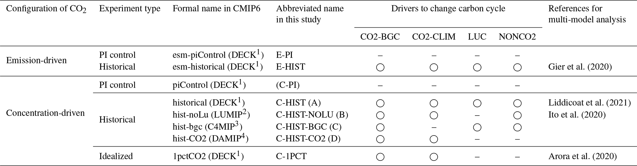
¹ “Diagnostic, Evaluation, and Characterization of Klima”, Eyring et al. (2016). ² “Land Use Model Intercomparison Project”, Lawrence et al. (2016). ³ “Coupled Climate–Carbon Cycle Model Intercomparison Project”, Jones et al. (2016). ⁴ “Detection and Attribution Model Intercomparison Project”, Gillett et al. (2016).

2.2 Models

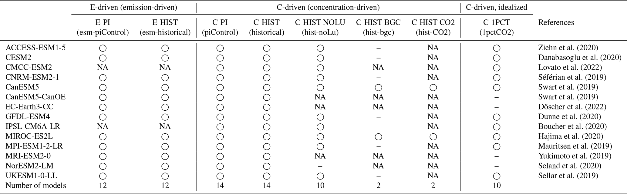
This study analyzed 12 CMIP6 ESMs for which simulation results of both C-HIST and E-HIST are available (Table 2). Furthermore, because land use change emission, which can be diagnosed from the C-HIST-NOLU experiment, is an important component of the global carbon budget, two ESMs (i.e., CMCC-ESM2 and IPSL-CM6A-LR) were added to the list of target models, although corresponding E-HIST results are unavailable.

2.3 Definition of analyzed variables and global carbon budget equations

The global carbon budget can be expressed using five terms:

$$E_{\mathrm{FF}}\left(t\right)+E_{\mathrm{LUC}}\left(t\right)=C_{\mathrm{A}}\left(t\right)+C_{\mathrm{O}}\left(t\right)+C_{\mathrm{LN}}\left(t\right),$$

where E_FF(t) is the cumulative emission from fossil fuels from 1850 to t; E_LUC(t) is that from net land use change (i.e., carbon emission derived from vegetation disturbances (e.g., deforestation and crop harvesting) minus carbon uptake by plant regrowth after the disturbances); and C_A(t), C_O(t), and C_LN(t) represent the change in carbon amount in the atmosphere, ocean, and natural land ecosystem, respectively. In this expression, C_LN(t) is equivalent to the cumulative carbon uptake by land where land use status is fixed at the preindustrial condition. Calculations of the cumulative values start from 1850. Hereafter, for concise expression, we drop the expression (t) from the above equation:

$$\begin{array}{}\text{(1a)}& E_{\mathrm{FF}}+E_{\mathrm{LUC}}=C_{\mathrm{A}}+C_{\mathrm{O}}+C_{\mathrm{LN}}.\end{array}$$

Using a term of land carbon change that includes land use change impact (C_L), this equation can be rewritten as follows:

$$\begin{array}{}\text{(1b)}& \begin{array}{rl}{E}_{\mathrm{FF}}=& C_{\mathrm{A}}+C_{\mathrm{O}}+\left(C_{\mathrm{LN}}-E_{\mathrm{LUC}}\right)=C_{\mathrm{A}}+C_{\mathrm{O}}+C_{\mathrm{L}},\\ & \text{where}{C}_{\mathrm{L}}=\left(C_{\mathrm{LN}}-E_{\mathrm{LUC}}\right).\end{array}\end{array}$$

In this expression, land use change emission E_LUC becomes implicit and is incorporated into C_L. In most cases, ESMs simulate land carbon fluxes in this way. See Appendix A for further details regarding the derivation of Eq. (1b).

On the basis of Eq. (1b), the method of simulation in the E-driven mode (i.e., the change in atmospheric CO₂ concentration is simulated explicitly) can be summarized as follows:

$$\begin{array}{}\text{(2)}& C_{\mathrm{A}}^{\text{E-HIST}}=E_{\mathrm{FF}}^{\mathrm{CMIP}\mathrm{6}\mathrm{F}}-\left(C_{\mathrm{O}}^{\text{E-HIST}}+C_{\mathrm{L}}^{\text{E-HIST}}\right),\end{array}$$

where the superscript E-HIST represents the historical experiment with the E-driven mode, and the superscript CMIP6F implies the forcing prescribed by CMIP6. Using this prescribed fossil fuel emission rate ($E_{\mathrm{FF}}^{\mathrm{CMIP}\mathrm{6}\mathrm{F}}$) and the prescribed land cover change, models simulate the change in atmospheric CO₂ concentration (presented here as atmospheric carbon burden change, $C_{\mathrm{A}}^{\text{E-HIST}}$) based on simulation of the land and ocean fluxes ($C_{\mathrm{O}}^{\text{E-HIST}}$ and $C_{\mathrm{L}}^{\text{E-HIST}}$, respectively) that are affected by the carbon cycle and other feedbacks.

The calculation of compatible fossil fuel emission in the C-driven historical experiment (C-HIST) can be expressed as follows:

$$\begin{array}{}\text{(3a)}& E_{\mathrm{FF}}^{\text{C-HIST}}=C_{\mathrm{A}}^{\mathrm{CMIP}\mathrm{6}\mathrm{F}}+C_{\mathrm{O}}^{\text{C-HIST}}+C_{\mathrm{L}}^{\text{C-HIST}}.\end{array}$$

By prescribing the CO₂ concentration (presented here as atmospheric carbon change, $C_{\mathrm{A}}^{\mathrm{CMIP}\mathrm{6}\mathrm{F}}$), models can simulate the ocean and land carbon fluxes ($C_{\mathrm{O}}^{\text{C-HIST}}$ and $C_{\mathrm{L}}^{\text{C-HIST}}$, respectively) that reflect both climate and carbon cycle feedbacks and the impacts from other external forcing. Through a posteriori summation of $C_{\mathrm{A}}^{\mathrm{CMIP}\mathrm{6}\mathrm{F}}$, $C_{\mathrm{O}}^{\text{C-HIST}}$, and $C_{\mathrm{L}}^{\text{C-HIST}}$, the cumulative value of the compatible fossil fuel emission $E_{\mathrm{FF}}^{\text{C-HIST}}$ can be diagnosed.

Table 2 List of participating CMIP6 ESMs and the experiment outputs used in this study. Circle symbols and “NA” represent model data availability and unavailability, respectively, for the experiments. The “–” symbol represents a model or experiment for which data are available but not analyzed in this study; C-HIST-BGC results from nine ESMs are available, but only two were used for analysis because the analysis needed both C-HIST-BGC and C-HIST-CO2 results; C-1PCT results are available for all ESMs, but this study used 10 models that also provided C-HIST-NOLU results; C-HIST-NOLU results of NorESM2-LM were not used in this study because of the quality of land carbon flux data in the experiment.

When the natural carbon uptake by land ($C_{\mathrm{LN}}^{\text{C-HIST}}$) and land use change emission ($E_{\mathrm{LUC}}^{\text{C-HIST}}$) can be assessed through a combination of other historical experiments (i.e., hist-noLu), this expression can be rewritten as follows:

$$\begin{array}{}\text{(3b)}& E_{\mathrm{FF}}^{\text{C-HIST}}=C_{\mathrm{A}}^{\mathrm{CMIP}\mathrm{6}\mathrm{F}}+C_{\mathrm{O}}^{\text{C-HIST}}+\left(C_{\mathrm{LN}}^{\text{C-HIST}}-E_{\mathrm{LUC}}^{\text{C-HIST}}\right).\end{array}$$

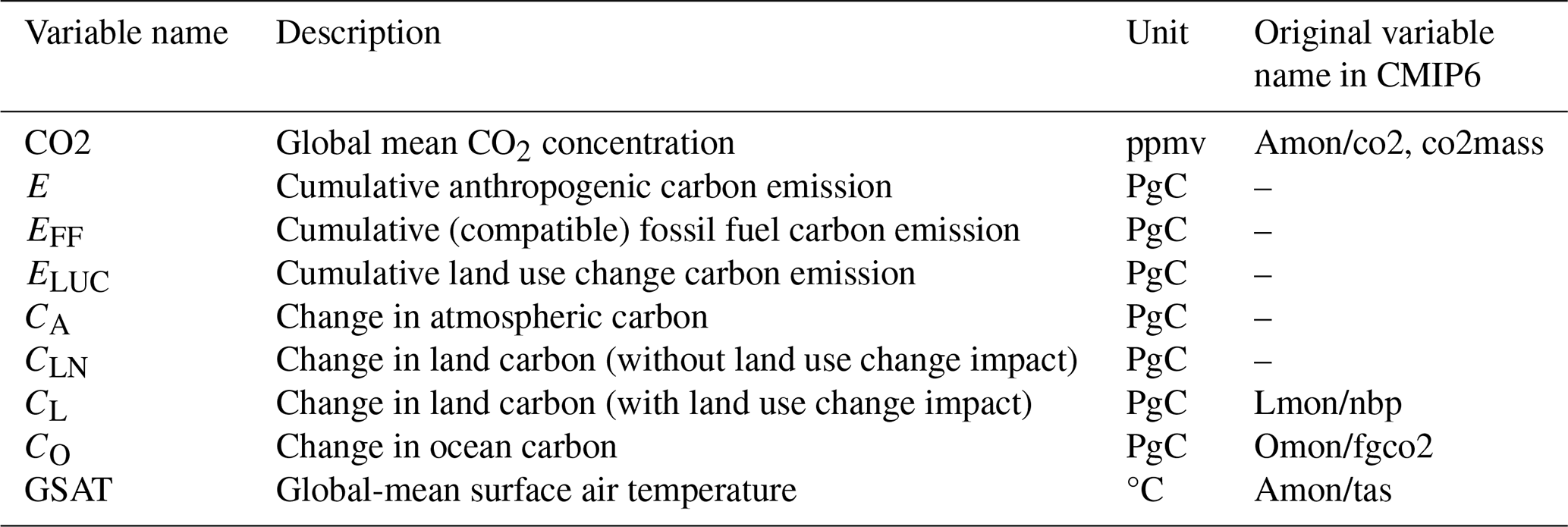
The analysis performed in this study was based on Eqs. (1)–(3), and three types of CMIP6 variables were used (Table 3). The first variable was atmospheric CO₂ concentration, which is the three-dimensional atmospheric CO₂ concentration, named “co2” in CMIP6. In this study, the globally averaged concentration (hereafter, “CO2”) was analyzed. Using this variable, C_A was calculated as $C_{\mathrm{A}}=\mathrm{\Delta }\mathrm{CO}\mathrm{2}\times \mathrm{2.124}$, where 2.124 is the ppmv–PgC conversion factor (Prather et al., 2012). If the co2 variable was unavailable, the global mass of atmospheric carbon, “co2mass”, was used instead in the analysis. The second and third variables, named nbp and fgco2 in CMIP6, represent the rate of CO₂ exchange between the atmosphere and the land biosphere and the ocean, respectively; in this analysis, these fluxes were analyzed after being converted to cumulative values, i.e., $\mathrm{\Delta }{C}_{\mathrm{L}}={\int }_{\mathrm{1850}}^t\mathrm{nbp}\mathrm{d}t$ and $\mathrm{\Delta }{C}_{\mathrm{O}}={\int }_{\mathrm{1850}}^t\mathrm{fgco}\mathrm{2}\mathrm{d}t$, respectively. As mentioned above, drift corrections were applied to these cumulative variables because the models are not necessarily fully equilibrated in the piControl run and because models sometimes assume additional natural sources and/or sinks of carbon (Appendix B).

Although the scope of this study focused primarily on global carbon cycle processes, it was considered to be valuable to compare the simulated global mean surface air temperature (hereafter, “GSAT”) between C-HIST and E-HIST. Therefore, GSAT was calculated from the “tas” variable in CMIP6, and drift correction was performed by evaluating the GSAT trend linearly in the preindustrial control experiment and subtracting the trend from the simulated GSAT in C-HIST and E-HIST (Fig. S1 in the Supplement).

Table 3 Definition of variables.

2.4 Analysis procedures and variables

The analysis procedures adopted are summarized in this section and illustrated in Figs. 1 and 2. Figure 1 summarizes the first stage of the multi-model comparison, the purpose of which was to confirm the level of consistency between the C-HIST and E-HIST experiments with regard to the fundamental terms of the global carbon budget. This stage consists of the following steps:

1. comparison of the prescribed fossil fuel emissions used for E-HIST ($E_{\mathrm{FF}}^{\mathrm{CMIP}\mathrm{6}\mathrm{F}}$) with compatible emissions obtained from the C-HIST experiment ($E_{\mathrm{FF}}^{\text{C-HIST}}$)

2. comparison of the prescribed CO₂ concentration used for C-HIST (CO2^CMIP6F) with the simulated concentration in E-HIST (CO2^E-HIST)

3. comparison of simulated ocean and land carbon uptake in C-HIST ($C_{\mathrm{O}}^{\text{C-HIST}}$ and $C_{\mathrm{L}}^{\text{C-HIST}}$, respectively) with those of E-HIST ($C_{\mathrm{O}}^{\text{E-HIST}}$ and $C_{\mathrm{L}}^{\text{E-HIST}}$, respectively)

4. comparison of GSAT between C-HIST and E-HIST (GSAT^C-HIST and GSAT^E-HIST, respectively).

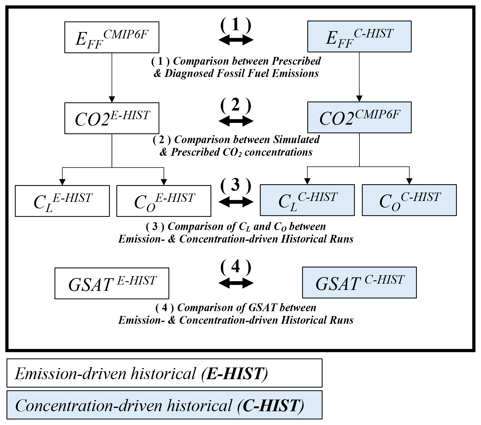
Figure 1 Analysis flow chart 1. The purpose of this series of analyses was to confirm the level of consistency between the historical E-driven experiments (E-HIST, left) and the C-driven experiments (C-HIST, right). Definitions of the variables and experiments can be found in Tables 1, 2, and 3. Solid arrows represent decomposition of the global carbon budget, and bold arrows with numbers represent comparison steps. All analyses were performed after removing the trend found in the preindustrial control experiments (C-PI and E-PI).

The second stage of the multi-model comparison, which consists of four steps, was designed to investigate the linkages of E-driven historical experiments with other C-driven experiments, as summarized in Fig. 2.

• 1.

  A potential linkage between the atmospheric CO₂ concentration simulated in the E-HIST experiment (CO2^E-HIST) and the compatible anthropogenic emissions of C-HIST ($E_{\mathrm{FF}}^{\text{C-HIST}}$; see Eq. 3a and Table 3) was investigated because both factors are important quantities in summarizing the carbon cycle processes in each experimental configuration.

• 2.

  Compatible fossil fuel emission ($E_{\mathrm{FF}}^{\text{C-HIST}}$) was compared to the diagnosed land use change emission ($E_{\mathrm{LUC}}^{\text{C-HIST}}$) in C-HIST to investigate the potential relationship between them in C-HIST because their negative correlation was identified in a previous study (Liddicoat et al., 2021). In this study, $E_{\mathrm{LUC}}^{\text{C-HIST}}$ was estimated by taking the difference between the results of C-HIST (normal historical simulations) and C-HIST-NOLU (historical simulation without land use change), as presented in Table 1 and Eqs. (3a) and (3b). We note that the method of diagnosis of land use change emission is under debate and that the $E_{\mathrm{LUC}}^{\text{C-HIST}}$ diagnosed in this study might yield a different magnitude of the cumulative emission compared with that of other approaches (Obermeier et al., 2021; Ciais et al., 2022).

• 3.

  $E_{\mathrm{FF}}^{\text{C-HIST}}$ depends on the magnitude of natural carbon sinks of the land and the ocean (Eq. 3b), which are affected by carbon cycle feedbacks. The carbon cycle feedbacks in models have been widely diagnosed using the idealized experiment C-1PCT. Thus, in this study, the magnitudes of the land and ocean natural sinks were compared between the realistic historical simulation (C-HIST) and the idealized experiment (C-1PCT). For this analysis, historical land carbon change without land use change impact ($C_{\mathrm{LN}}^{\text{C-HIST}}$, which is equivalent to $C_{\mathrm{L}}^{\text{C-HIST-NOLU}}$) was required because land carbon change is simulated in the idealized experiment in this way.

• 4.

  After performing step (3), to confirm the reasons for establishing clear or non-clear relationships between the historical and the idealized experiments, the changes in land and ocean carbon were decomposed into the changes caused by four types of drivers, namely

  • i.

    carbon change induced by CO₂–carbon feedback (CO2-BGC)

  • ii.

    carbon change induced by climate–carbon feedback caused by CO₂-induced warming (CO2-CLIM)

  • iii.

    carbon change induced by land use change (LUC)

  • iv.

    carbon change induced by non-CO₂ effects (NONCO2).

The carbon changes induced by the four drivers can be diagnosed by taking into account the differences between four types of historical simulations (C-HIST, C-HIST-NOLU, C-HIST-BGC, and C-HIST-CO2; Table 1; see Appendix C for the detailed methodology). However, because of data availability, this analysis was applied to only two models: CanESM5 and MIROC-ES2L.

On the basis of the analysis steps, the linkages between the C-HIST and E-HIST historical experiments were investigated. In the analysis, it was assumed that the major difference between the two types of experimental configurations reflects whether the simulated carbon fluxes change the CO₂ concentration (E-HIST) or not (C-HIST). We note, however, that there could be other reasons that might cause systematic differences in the carbon cycle behavior between the two types of experiment. First, the CO₂ concentration in E-HIST is usually simulated using a three-dimensional field with sub-daily time steps, while that in C-HIST might be spatially homogeneous or longitudinally averaged with annual or seasonal time steps. This might affect the geographical and seasonal pattern of natural carbon sinks. Second, because of the difference in the spatial distribution of CO₂ concentration, the radiative forcing that arises from CO₂ might also be different between the two types of experiments, affecting the meteorological conditions over the land and ocean surfaces and altering carbon cycle and/or biophysical feedbacks. Finally, because of the differences mentioned above, the spin-up procedure is usually performed separately for each experiment, and the spin-up duration might be different. This can cause different initial states in the climate and the carbon cycle system between C-HIST and E-HIST that might affect the historical change in the global carbon budget.

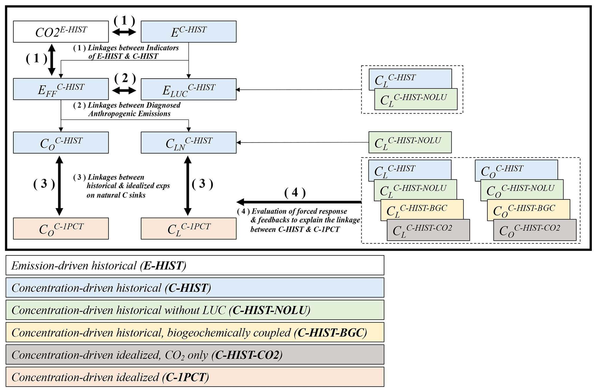
Figure 2 Analysis flow chart 2. The purpose of this series of analyses was to investigate the linkages between E-driven historical experiments and other C-driven experiments. Solid arrows represent decomposition of the global carbon budget, and bold arrows with numbers represent comparison steps. Definitions of the variables and experiments can be found in Tables 1, 2, and 3. All analyses were performed after removing the trend found in the preindustrial control experiments (C-PI and E-PI).

3 Results and discussion

3.1 Result of analysis 1: consistency between emission- and concentration-driven historical simulations

3.1.1 Multi-model means

The results of analysis 1 (Fig. 1), i.e., the comparison between C-HIST and E-HIST experiments with regard to the basic components of the global carbon budget, are shown in Table 4, Fig. 3 (multi-model averages), and Fig. S2 (individual model results). In Table 4, the global carbon budgets are presented as cumulative values (except for CO₂ concentration) during 1850–2014. Inspection of Fig. 3 confirms that the multi-model averages of C-HIST and E-HIST generally show reasonable agreement for the temporal changes in fossil fuel and land use emission, CO₂ concentration, and carbon uptake by the ocean and by the land. However, several discrepancies exist between the two experiments. First, the multi-model average of compatible fossil fuel emission is 374 PgC, which is smaller by 35 PgC than that used as the prescribed emission for E-HIST (Fig. 3a). Second, during 1900–1950, the carbon budget components of fossil fuel emission (Fig. 3a), change in CO₂ concentration (Fig. 3b), and carbon uptake by the land and by the ocean (Fig. 3c and d) in E-HIST are slightly smaller than those in C-HIST. This suggests that it is difficult for E-HIST to reproduce the CO₂ concentration plateau observed in ice core measurements, which is discussed later. Third, the multi-model average of simulated CO₂ concentration at the end of E-HIST is 405 ppmv, which is larger by approximately 7 ppmv than that of the prescribed concentration used for C-HIST (Fig. 3b). Fourth, because of the variation in simulated CO₂ concentration between the models (405 ± 14.4 ppmv in 2014), E-HIST exhibits larger spread in terms of GSAT (by 30 %) than C-HIST, in which models use a common CO₂ concentration pathway (Fig. 3e).

In comparison with the numbers reported in the best estimates of the global carbon budget, i.e., GCB2021, the multi-model average of compatible fossil fuel emission diagnosed from C-HIST is smaller by approximately 26 PgC (Table 4 and Fig. 3a). Additionally, the prescribed fossil fuel emission used for E-HIST has minor discrepancies with GCB2021. In CMIP6, the emissions were based on a Community Emissions Data System approach (Hoesly et al., 2018) that produces CO₂ emissions that are consistent with all the other species. Fundamentally, the Community Emissions Data System is sector-based and not fuel-based; consequently, the cumulative CMIP6 emissions are higher than the GCB2021 emissions by approximately 10 PgC (Table 4; Andrew, 2020), mainly in the period 1950–1999. Moreover, the total anthropogenic CO₂ emissions in CMIP6 consisted of the sum of all sectors in the two-dimensional files and the three-dimensional emissions in the aircraft CO₂ emissions files. Although most modeling groups likely used this summation to force emission-driven experiments, some might have neglected the aviation emissions, and the corresponding discrepancy in the simulated atmospheric CO₂ concentration by 2014 could be of the order of several parts per million.

The multi-model average of land use change emission, which was diagnosed by taking the difference between C-HIST and C-HIST-NOLU, is 129 PgC, which is much smaller (by approximately 65 PgC) than that of the GCB2021 estimation (Table 4 and Fig. 3a). This large discrepancy between the CMIP6 ESMs and GCB2021 might arise from the different assumptions, definitions, or approaches adopted for the land use change emission. In the CMIP6 simulations, the land use change emission is interactively computed in the transient historical simulation. Thus, the emission calculation is subject to the effect of environmental changes; e.g., carbon emission from deforestation and carbon uptake through forest regrowth are simulated under time-varying CO₂ concentrations and climate change. Additionally, the models analyzed here for land use change emissions (Table 4), except for the three models of GFDL-ESM4, MIROC-ES2L, and MPI-ESM1-2-LR, consider net land use changes; i.e., concurrent, bidirectional transformations between land use types within a grid cell are not considered (Ito et al., 2020). This might lead to underestimation of the magnitude of land use change emission, as highlighted previously (e.g., Ciais et al., 2022; Friedlingstein et al., 2021). Meanwhile, GCB2021 adopts a bookkeeping method for estimating the land use change emission with gross transition of land use changes. The method usually assumes constant biomass throughout the historical period for the emission calculation; however, because contemporary biomass is used for the calculation, the emission from deforested biomass and the loss of additional carbon sinks could be larger than in the ESM simulations (Obermeier et al., 2021; Friedlingstein et al., 2021).

The natural land carbon sink is simulated by the CMIP6 ESMs to be 148 ± 31 PgC (C-HIST-NOLU), whereas GCB2021 has a value of 180 ± 40 PgC (Table 4 and Fig. 3c). The ocean carbon sink is simulated to be 137 ± 11 PgC in C-HIST and 145 ± 17 PgC in E-HIST, both of which are slightly lower than the GCB2021 estimate of 150 ± 30 PgC (Table 4 and Fig. 3d).

We note that simulated climate variability could change the magnitudes of simulated CO₂ uptakes, causing different magnitudes of cumulative land and ocean uptakes in different ensemble members of the historical experiment. However, examination using multiple ensemble members of C-HIST, performed using MIROC-ES2L (30 members) and UKESM-1-0-LL (12 members), reveals that the impact of internal climate variability on these cumulative quantities is small (Table S1). The multi-ensemble spread of cumulative terrestrial carbon uptake is ± 4.1 PgC for MIROC-ES2L and ± 4.1 PgC for UKESM, which is approximately only 6 % of the multi-model spread (± 74.2 PgC; Table 4); for the ocean, the multi-ensemble spread is confirmed to be ± 0.8 PgC for MIROC-ES2L and ± 1.4 PgC for UKESM, i.e., both substantially smaller than the multi-model spread of ± 10.7 PgC.

Table 4 Global carbon budget simulated in concentration- and emission-driven historical simulations (C-HIST and E-HIST, respectively) as performed by CMIP6 ESMs and the difference (“diff.”). Results of global mean surface air temperature (GSAT) are also presented. Note that these results are based on a single simulation of each C- and E-driven historical experiment. The analysis corresponds to steps (1), (2), (3), and (4) shown in Fig. 1. The simulated period is 1850–2014, and the results of the global carbon budgets are quantified as cumulative values and evaluated at the end of the historical simulation. GSAT is presented by the anomalies of GSAT (2005–2014 average). Definitions of the variables and the experiments can be found in Tables 1, 2, and 3. Corresponding GCB2021 values are also presented at the bottom of the table. Unavailability of data is represented by the “–” symbol.

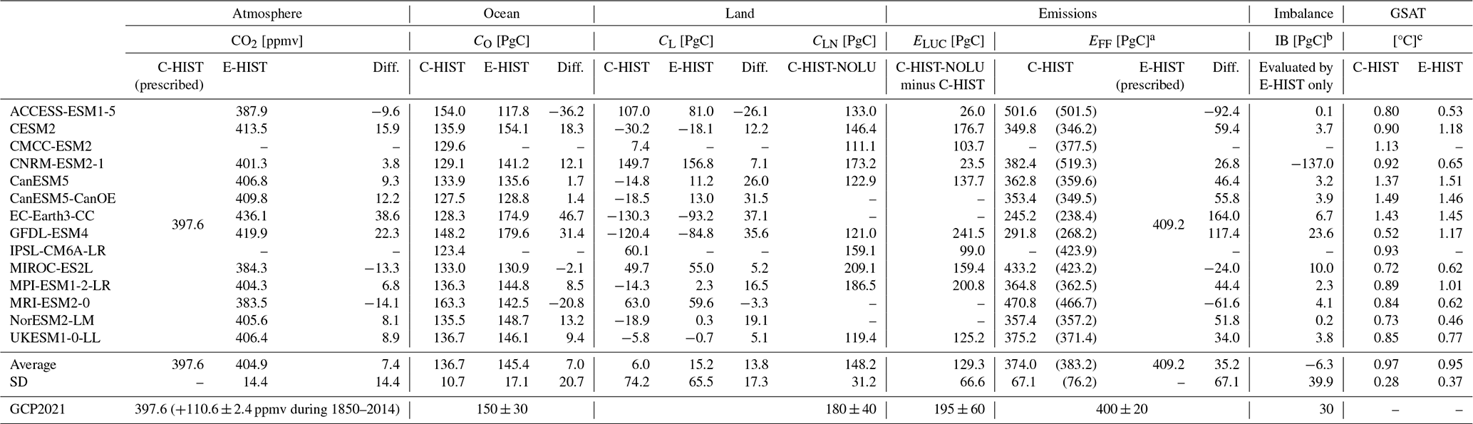
^a Compatible fossil fuel emission $E_{\mathrm{FF}}^{\text{C-HIST}}$ is modified by the imbalance term IB (i.e., $E_{\mathrm{FF}}^{\text{C-HIST}}=$ (397.6−284.3) × 2.124 + $C_{\mathrm{O}}^{\text{C-HIST}}+C_{\mathrm{L}}^{\text{C-HIST}}+$ IB), and the $E_{\mathrm{FF}}^{\text{C-HIST}}$ before the IB correction is shown in parentheses. ^b The imbalance term IB is evaluated using the E-HIST result as IB = 409.2−ΔCO${}_{\mathrm{2}}^{\text{E-HIST}}$ × $\mathrm{2.124}-C_{\mathrm{O}}^{\text{E-HIST}}-C_{\mathrm{L}}^{\text{E-HIST}}$. ^c Corrected by the GSAT drift that is found in the corresponding preindustrial control simulations (Fig. S1).

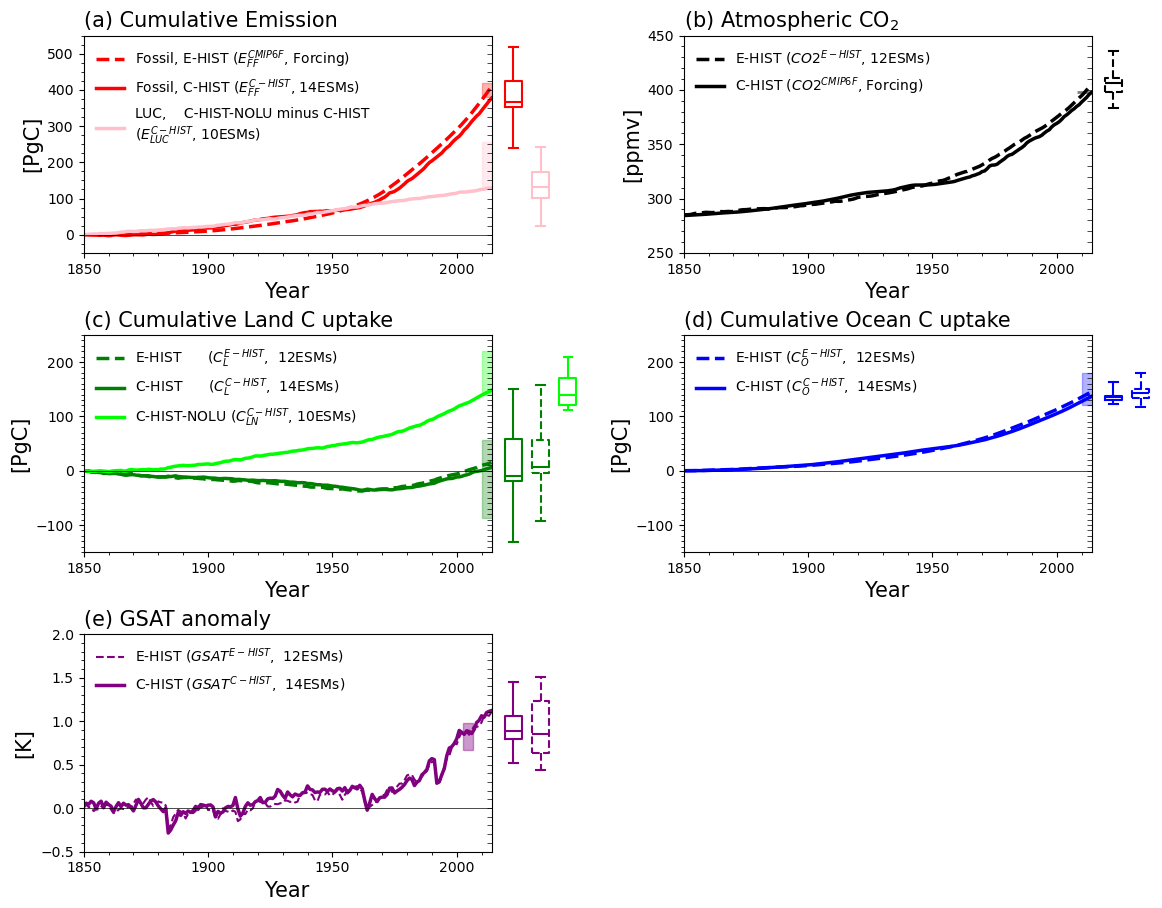
Figure 3 Consistency of global carbon budget and anomaly of global mean surface air temperature (GSAT) between C-driven and E-driven CMIP6 historical (1850–2014) simulations (i.e., C-HIST and E-HIST, respectively), shown by the multi-model means of the ESMs. This analysis corresponds to steps (1), (2), (3), and (4) shown in Fig. 1. Simulated results of C-HIST and E-HIST are represented by solid lines and dashed lines, respectively, in panels (a), which represents cumulative anthropogenic emission E_FF before the imbalance correction; (b), which represents atmospheric CO₂ concentration CO2; (c), which represents cumulative land carbon uptake with (C_L, dark green) and without (C_LN, light green) consideration of the impact of land use change; (d), which represents cumulative ocean carbon uptake C_O; and (e), which represents the anomaly of GSAT. Vertical bars within panels (a)–(d) show the estimation range from GCB2021. The vertical bar within panel (e) reflects reference data obtained from Gulev et al. (2021), showing the GSAT change presented by an anomaly from 1850–1900 to 1995–2014. In panels (a) and (b), fossil fuel emission for the E-driven run and CO₂ concentration for the C-driven run, respectively, are obtained from the prescribed forcing datasets used for CMIP6. In the boxplots, the bottom and top caps represent the minimum and maximum model results (no outlier), respectively, and the bottom and top ends of the boxes represent the 25th and 75th percentiles, respectively; horizontal lines in the boxes represent the median (50th percentile); the numbers for 2014 are used in the boxplots in panels (a)–(d), and the 2005–2014 average is used in panel (e). A similar plot confirming the individual model results is shown in Fig. S2.

3.1.2 Individual models

Although the multi-model averages have been confirmed to show general agreement between C-HIST and E-HIST, the simulation results of each individual model sometimes show large differences between the two types of experiments (Fig. 4). First, although land carbon uptake (C_L) in each model shows similar magnitudes between the two experiments (R²=0.97; Fig. 4), ocean carbon uptake (C_O) shows weak correlation (C_O, R²=0.01; Fig. 4b), suggesting that ocean carbon uptake of E-HIST cannot be well explained by that of C-HIST in some models. This is likely due to differences in the experimental configurations. In E-HIST, the land carbon flux, the magnitude of which is estimated very differently by the models and forced to change by the prescribed land cover dataset, changes the simulated atmospheric CO₂ concentration. Thus, models with land carbon uptake that is too strong likely simulate lower CO₂ concentrations, leading to a weaker ocean carbon sink through the CO₂–oceanic carbon feedback process. This mechanism makes the ocean carbon uptake dependent on the land carbon uptake (R²=0.56; Fig. 4d), yielding a different magnitude of ocean carbon uptake between E-HIST and C-HIST. Meanwhile, in C-HIST, the land and ocean carbon fluxes do not change the CO₂ concentration, and, thus, the land carbon flux in the models does not affect the ocean carbon sink, resulting in independent behavior of the land and ocean carbon fluxes (R²=0.01; Fig. 4c). Additionally, the spatial distribution and the seasonality of the prescribed CO₂ concentration used for C-HIST are lost or latitudinally fixed, while the concentration field in E-HIST is freely simulated by the models. To some extent, this might be another reason for the yielding of different magnitudes of the ocean carbon sink between C-HIST and E-HIST (Halloran, 2012).

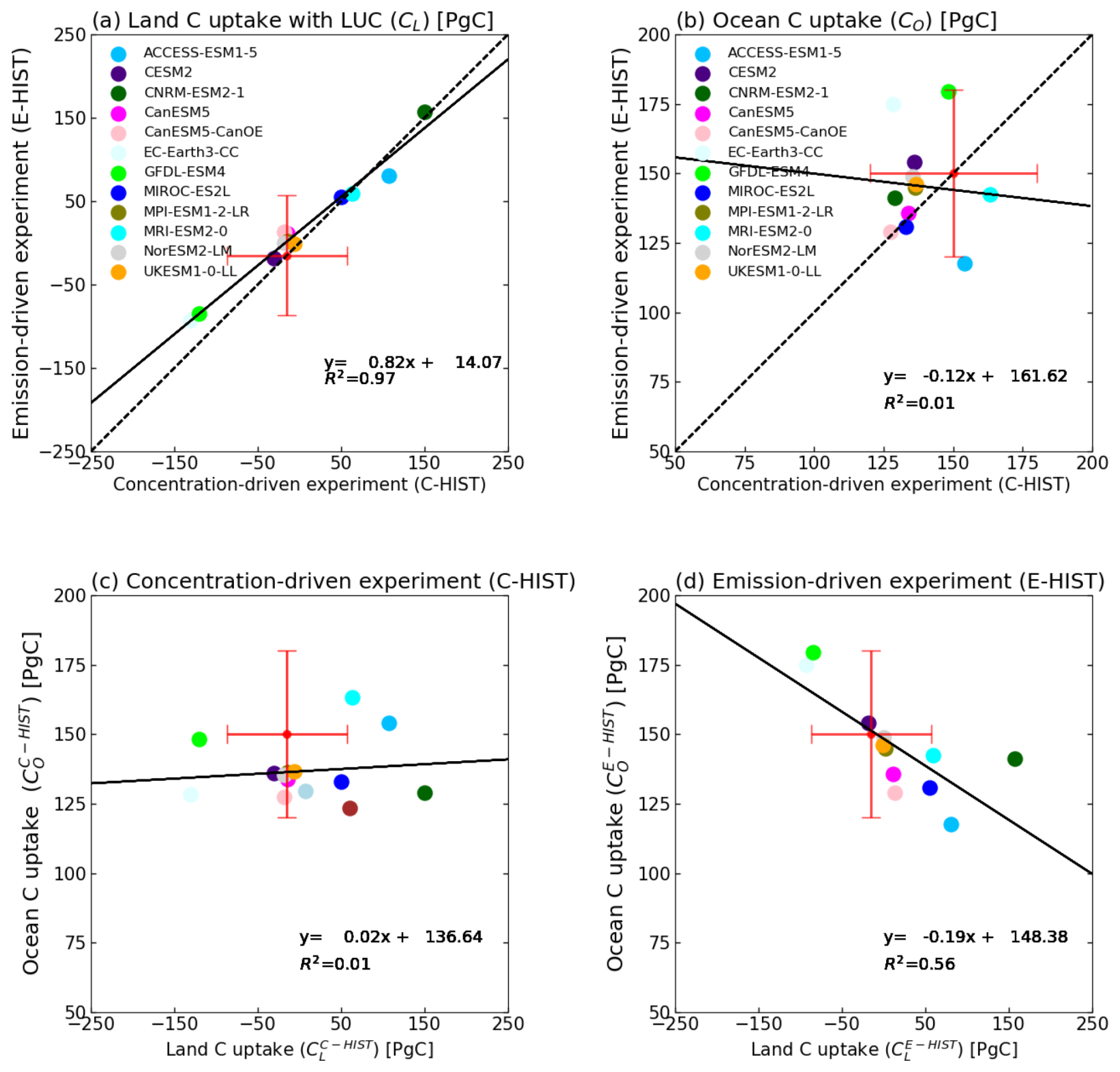
Figure 4 Comparison of cumulative carbon uptakes by land and ocean between the C-driven and E-driven historical (1850–2014) experiments (i.e., C-HIST and E-HIST, respectively) simulated by CMIP6 ESMs. This analysis corresponds to step (3) in Fig. 1, and the comparison is made at the end of the historical simulations. The two types of historical simulations are compared with regard to (a) cumulative land carbon uptake C_L and (b) cumulative ocean carbon uptake C_O. The dependency between the carbon uptake of the land and of the ocean in each experiment is shown in (c) for C-HIST and (d) for E-HIST. Solid and dashed lines represent the regression line and the 1:1 line, respectively. Red bars represent the range of uncertainty obtained from GCB2021 (Friedlingstein et al., 2021); it should be noted that GCB2021 does not report land carbon uptake with a consideration of the impact of land use change (C_L), and, thus, it is estimated here as $C_{\mathrm{L}}=C_{\mathrm{LN}}-E_{\mathrm{LUC}}$ and ${\mathit{\sigma }}_{\mathrm{CL}}^{\mathrm{2}}={\mathit{\sigma }}_{\mathrm{CLN}}^{\mathrm{2}}+{\mathit{\sigma }}_{\mathrm{ELUC}}^{\mathrm{2}}$.

3.2 Result of analysis 2: linkages of CO₂ concentration in E-driven experiment with other variables in C-driven experiments

In the analysis in Sect. 3.1, we compared the fundamental terms of the global carbon budget between C-HIST and E-HIST. In the following, on the basis of the analytical procedure shown in Fig. 2, the linkages between E-HIST and several types of C-driven experiment are investigated.

3.2.1 Diagnosed anthropogenic emissions ($E_{\mathrm{FF}}^{\text{C-HIST}}$) and simulated CO₂ concentration (CO${}_{\mathrm{2}}^{\text{E-HIST}}$)

In Fig. 5, the simulated CO₂ concentration for 2014 in E-HIST (CO2^E-HIST) is plotted against the cumulative anthropogenic CO₂ emissions ($E_{\mathrm{FF}}^{\text{C-HIST}}$ and $E_{\mathrm{LUC}}^{\text{C-HIST}}$) diagnosed from C-HIST following step (1) in Fig. 2. As mentioned in Sects. 1 and 2, $E_{\mathrm{FF}}^{\text{C-HIST}}$ can be considered to be an indicator that aggregates carbon cycle feedbacks and the response to environmental change in C-HIST, while CO2^E-HIST is applicable to E-HIST. It should be noted that we used the compatible fossil fuel emission $E_{\mathrm{FF}}^{\text{C-HIST}}$ that is corrected by the carbon budget imbalance found in each model (IB column in Table 4) because CO2^E-HIST and $E_{\mathrm{FF}}^{\text{C-HIST}}$ should be compared with the equivalent quality (Appendix B).

In Fig. 5a, the compatible fossil fuel plus the simulated land use change emission ($E_{\mathrm{FF}}^{\text{C-HIST}}+E_{\mathrm{LUC}}^{\text{C-HIST}}$) is used to explain CO2^E-HIST; in Fig. 5b, the compatible fossil fuel emission ($E_{\mathrm{FF}}^{\text{C-HIST}}$) alone is used as the explanatory variable. In the analysis, $E_{\mathrm{FF}}^{\text{C-HIST}}+E_{\mathrm{LUC}}^{\text{C-HIST}}$ does not explain CO2^E-HIST well (R²=0.05), whereas using $E_{\mathrm{FF}}^{\text{C-HIST}}$ alone shows strong correlation (R²=0.91). In E-HIST, the strength of carbon cycle feedbacks and the magnitude of land use change emission in the models determine the CO₂ concentration (y axis of Fig. 5b). In C-HIST, however, the strength of feedbacks and the land use change emission are reflected in the compatible fossil fuel emission (x axis of Fig. 5b) by definition (Eq. 3b); consequently, models that have strong land use change emission should have lower compatible emission, which is discussed later. Thus, using only the compatible fossil fuel emission of C-HIST better explains the magnitude of the CO₂ concentration in E-HIST.

It is evident that CO2^E-HIST and $E_{\mathrm{FF}}^{\text{C-HIST}}$ are anticorrelated (Fig. 5b), and the slope of the regression line is −0.20 ppmv PgC⁻¹, which is equivalent to a cumulative airborne fraction of −0.47 PgC PgC⁻¹. Thus, models with larger compatible fossil fuel emission in C-HIST have a lower simulated CO₂ concentration in E-HIST. Interestingly, the observed concentration and the fossil fuel emission reported in GCB2021 almost plot on the regression line, providing an important indication that models with an adequate cumulative compatible fossil fuel emission value (400 PgC) will simulate a CO₂ concentration that is sufficiently close to the observed value (397.6 ppmv). However, there is only one model that can simulate the compatible fossil fuel emission within the range of the GCB2021 values, i.e., CNRM-ESM2-1 (382.4 PgC). Consequently, most models overestimate or underestimate the concentration by more than 5 ppmv (Fig. 5b and Table 4). Further details targeting specific models can be found in Sect. S1 and Fig. S6 in the Supplement.

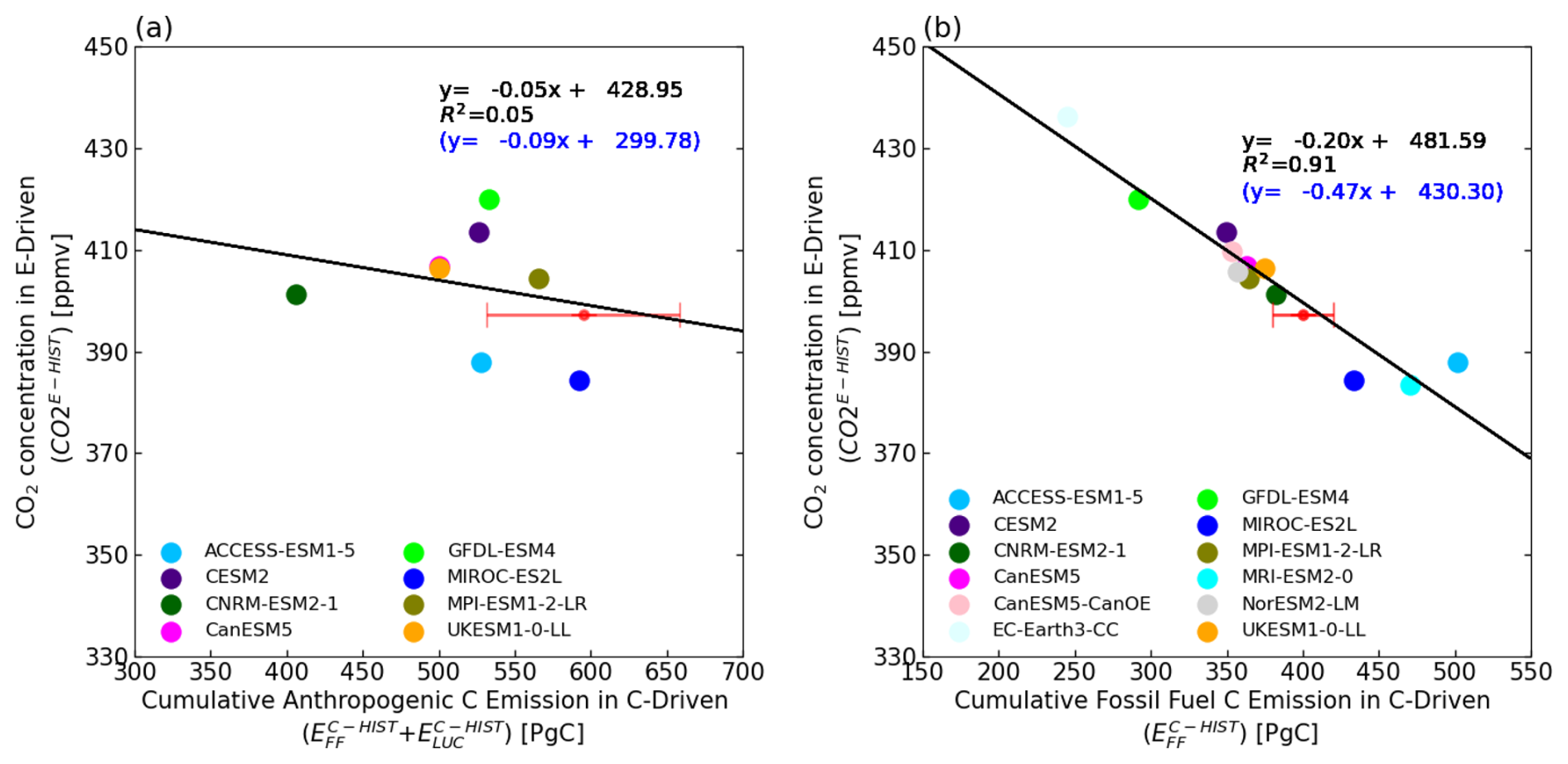
Figure 5 Comparison of CO₂ concentration in the E-driven historical run CO2^E-HIST with cumulative values of (a) total anthropogenic (i.e., compatible fossil fuel and land use change, $E_{\mathrm{FF}}^{\text{C-HIST}}+E_{\mathrm{LUC}}$) emission and (b) compatible fossil fuel emission $E_{\mathrm{FF}}^{\text{C-HIST}}$ alone. This analysis corresponds to step (1) in Fig. 2, and the comparison is made at the end of the historical simulations for 2014. The solid line represents the regression line (the equation in black represents the regression using atmospheric CO₂ concentration, and the equation in blue denotes the regression result that uses atmospheric carbon loading as the dependent variable). The red bars represent the range of uncertainty obtained from GCB2021 (Friedlingstein et al., 2021). The number of models reflects the availability of simulation results necessary for the analysis. Note that the compatible emissions were corrected using the imbalance term found in each model, and the plot before the correction is shown in Fig. S3.

3.2.2 Diagnosed emissions of fossil fuel ($E_{\mathrm{FF}}^{\text{C-HIST}}$) and land use change ($E_{\mathrm{LUC}}^{\text{C-HIST}}$)

In the next step, we compare two types of anthropogenic emission, i.e., fossil fuel ($E_{\mathrm{FF}}^{\text{C-HIST}}$) emission and land use change ($E_{\mathrm{LUC}}^{\text{C-HIST}}$) emission (step 2 in Fig. 2) in C-HIST, and the result is shown in Fig. 6. As reported by Liddicoat et al. (2021), the two variables in C-HIST show an anticorrelation relationship (R²=0.56). This is because, by replacing $C_{\mathrm{A}}^{\mathrm{CMIP}\mathrm{6}\mathrm{F}}+C_{\mathrm{O}}^{\text{C-HIST}}+C_{\mathrm{LN}}^{\text{C-HIST}}$ with S in Eq. (3b), the equation for the global carbon budget can be rewritten as $E_{\mathrm{FF}}^{\text{C-HIST}}=S-E_{\mathrm{LUC}}^{\text{C-HIST}}$. This equation suggests an underlying mechanism for the creation of the negative correlation between $E_{\mathrm{FF}}^{\text{C-HIST}}$ and $E_{\mathrm{LUC}}^{\text{C-HIST}}$; i.e., a model with higher land use change emission will yield lower fossil fuel emission to achieve the same CO₂ increase over the historical period (we note that $C_{\mathrm{O}}^{\text{C-HIST}}$, $C_{\mathrm{LN}}^{\text{C-HIST}}$, and $E_{\mathrm{LUC}}^{\text{C-HIST}}$ are confirmed to be independent of each other). Because the term S is not constant and differs among the various models, the individual models do not lie directly on the regression line. Comparison with GCB2021 reveals that no model can reproduce values of $E_{\mathrm{FF}}^{\text{C-HIST}}$ and $E_{\mathrm{LUC}}^{\text{C-HIST}}$ that are simultaneously within the range suggested by GCB2021.

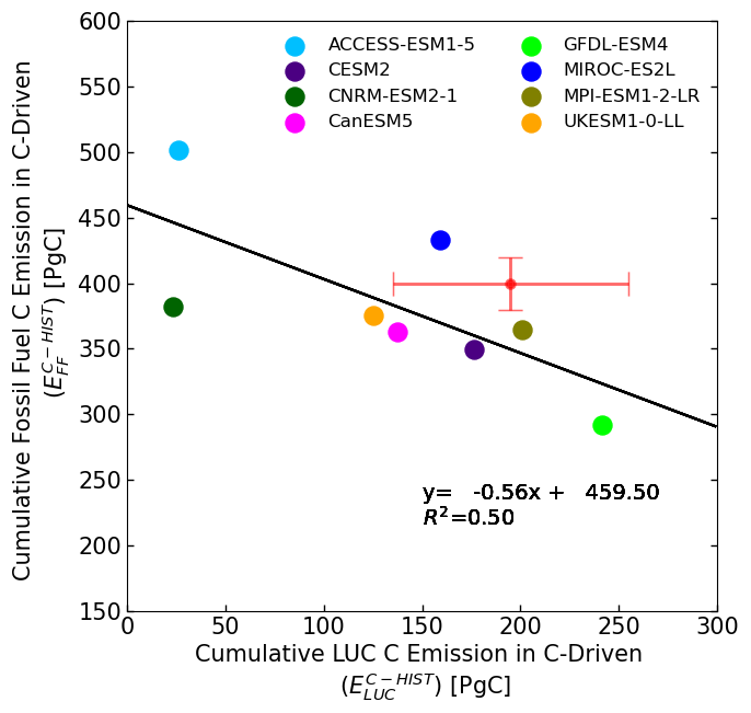
Figure 6 Comparison of cumulative land use change emission $E_{\mathrm{LUC}}^{\text{C-HIST}}$ and compatible fossil fuel emission $E_{\mathrm{FF}}^{\text{C-HIST}}$ in the C-driven historical run; land use change emission is diagnosed from a combination of C-HIST and C-HIST-NOLU. This analysis corresponds to step (2) in Fig. 2, and the comparison is made at the end of the historical simulations. The solid line represents the regression line, and the red bars represent the range of uncertainty obtained from GCB2021 (Friedlingstein et al., 2021). Note that the compatible emissions were corrected using the imbalance term found in each model, and the result before the correction is shown in Fig. S4.

3.2.3 Natural carbon sinks of land (C_LN) and ocean (C_O) in C-HIST and C-1PCT

The analysis above confirms, as expected, that diagnosed compatible fossil fuel emissions in the C-HIST experiment are affected by the magnitude of the land use change emissions simulated by the models. Additionally, the magnitude of the compatible fossil fuel emissions is also controlled by the magnitude of the simulated natural carbon sinks ($C_{\mathrm{LN}}^{\text{C-HIST}}$ for land and $C_{\mathrm{O}}^{\text{C-HIST}}$ for ocean, Eq. 3b), both of which are strongly affected by the magnitude of the CO₂–carbon and climate–carbon feedbacks. Here, we compare the simulated natural sinks over land ($C_{\mathrm{LN}}^{\text{C-HIST}}$) and ocean ($C_{\mathrm{O}}^{\text{C-HIST}}$) in the C-HIST experiment with those simulated in the idealized C-1PCT experiment, as illustrated in step (3) of Fig. 2. This comparison examines the linkages between the realistic historical experiment and the idealized experiment, where the latter is configured to analyze the carbon cycle feedbacks of the ESMs.

The comparison is made between the end of the C-HIST simulation (397.6 ppmv) and the 34th year of C-1PCT (398.8 ppmv). The results illustrated in Fig. 7a show that the natural ocean carbon sink has a positive correlation between C-HIST and C-1PCT (R²=0.81). This suggests that the magnitude of the natural ocean sink in C-HIST could be approximated from that in C-1PCT, although the magnitudes of the sinks differ owing to the different rate of CO₂ increase assumed in the scenarios. Conversely, the historical natural land carbon sink, which is obtained from C-HIST-NOLU, shows weak correlation with the idealized experiment (R²=0.07, Fig. 7b), although a systematic trend that models with higher $C_{\mathrm{L}}^{C-\mathrm{1}PCT}$ tend to have larger $C_{\mathrm{LN}}^{\text{C-HIST}}$ is confirmed. This suggests that the C-1PCT results, which have been widely used to investigate the carbon cycle feedbacks of the models, cannot be extrapolated to the C-HIST results in terms of the natural land carbon sink.

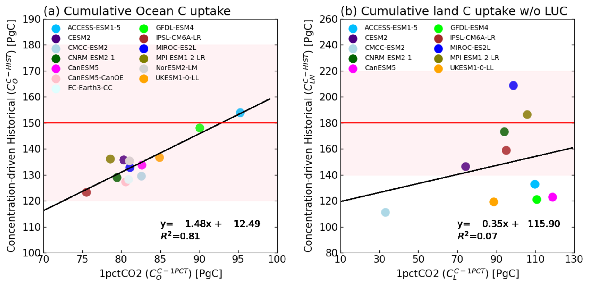
Figure 7 Comparison between the idealized experiment with a 1 % CO₂ increase (C-1PCT) and the C-driven historical experiment (C-HIST): (a) cumulative ocean carbon uptake ($C_{\mathrm{O}}^{\text{C-HIST}}$ versus $C_{\mathrm{O}}^{\text{C-1PCT}}$) and (b) cumulative land carbon uptake without a consideration of land use change ($C_{\mathrm{LN}}^{\text{C-HIST}}$ versus $C_{\mathrm{L}}^{\text{C-1PCT}}$, where $C_{\mathrm{LN}}^{\text{C-HIST}}$ is obtained as $C_{\mathrm{L}}^{\text{C-HIST-NOLU}}$). This analysis corresponds to step (3) in Fig. 2. The comparison is made at the end of the C-HIST simulation (397.6 ppmv) and in the 34th year of C-1PCT (398.8 ppmv). The solid lines represent the regression lines. The horizontal red line identifies the corresponding GCB2021 values, and the red-shaded area shows the range of uncertainty.

3.2.4 Possible reasons to make strong or weak linkages of natural carbon sinks between C-HIST and C-1PCT

To investigate the reason why a strong correlation between C-HIST and C-1PCT was found in ocean carbon uptake but not in land carbon uptake (Fig. 7), the cumulative carbon uptake by land and ocean was decomposed into the changes attributable to four types of drivers (i.e., CO2-BGC, CO2-CLIM, LUC, and NONCO2; analysis step (4) of Fig. 2; Appendix C). As described in the Methods section, this decomposition requires four types of historical experiments, and data availability limits the models to only CanESM5 and MIROC-ES2L. However, these two models are distinctive in the plotting space of Fig. 7b. Namely, CanESM5 is the model that shows the largest land carbon accumulation in C-1PCT, whereas MIROC-ES2L is the largest in C-HIST. Thus, analysis of these two models would elucidate the underlying mechanism that created the lack of correlation in land carbon uptake between C-HIST and C-1PCT.

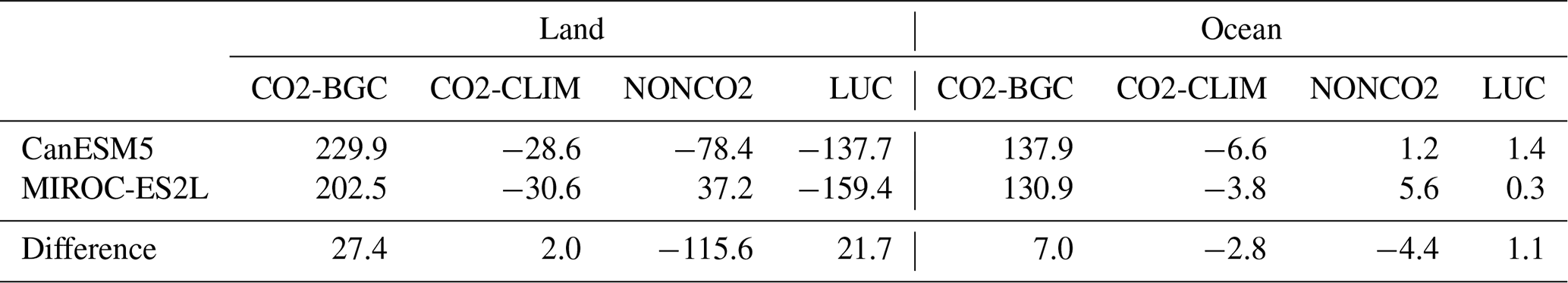
The results listed in Table 5 represent the cumulative values in 2014. For the ocean, we found that the CO2-BGC effect, which refers to carbon change via CO₂–carbon feedbacks, is almost comparable between the two models (137.9 PgC for CanESM5 and 130.9 PgC for MIROC-ES2L). Additionally, the ocean is mainly governed by the CO2-BGC effect, and the other three drivers (i.e., CO2-CLIM, NONCO2, and LUC) were diagnosed as being minor, i.e., < 5 PgC in terms of their absolute value. The analysis clearly shows that ocean carbon uptake in C-HIST is dominated by CO₂–carbon feedback on the global scale, as confirmed in C-1PCT (Arora et al., 2020); this can be expected from the formulation of ocean carbon flux, the modeling of which is more directly linked with the atmospheric CO₂ concentration (Hauck et al., 2020) than land (Ruehr et al., 2023). Because this dominance is common in both C-HIST and C-1PCT, a strong linkage was likely to be created for the ocean carbon uptake between the two experiments (Fig. 7a).

On land, the cumulative carbon change induced by CO2-BGC was largest in both models (229.9 PgC for CanESM5 and 202.5 PgC for MIROC-ES2L); however, the impact of each of the other three drivers was non-negligible. CO2-CLIM, which represents the carbon change caused by CO₂-induced warming, showed a moderate impact on land carbon uptake, with a very similar magnitude between the models (−28.6 PgC for CanESM5 and −30.6 PgC for MIROC-ES2L). The effect of LUC was evaluated to reduce land carbon by 137.7 PgC in CanESM5 and by 159.4 PgC in MIROC-ES2L (values that are identical to the cumulative values of land use change emission listed in Table 4). NONCO2 is the carbon change induced by warming or cooling from non-CO₂ greenhouse gases and aerosols (Jones et al., 2003), and it also includes the direct stimulation of land biogeochemistry via nutrient inputs (e.g., nitrogen deposition). This NONCO2 effect showed moderate impacts in both models, but the signs were different (i.e., −78.4 PgC for CanESM5 and +37.2 PgC for MIROC-ES2L), leading to the largest discrepancy of 115.6 PgC between the two models. Because the NONCO2 effect is active in C-HIST and C-HIST-NOLU but absent in the C-1PCT experiment (Table 1), this is the main reason for the remarkable difference in land carbon uptake between CanESM5 and MIROC-ES2L (Fig. 7b). This might also be true for other models and might explain the weak linkage between $C_{\mathrm{LN}}^{\text{C-HIST}}$ and $C_{\mathrm{L}}^{\text{C-1PCT}}$ in CMIP6 ESMs.

Table 5 Changes in natural carbon fluxes integrated over the entire historical period (1850–2014), presented by four drivers (unit: PgC). Positive numbers represent carbon uptake by land or ocean. This analysis corresponds to step (4) in Fig. 2.

4 Suggestions for improved simulation of CO₂ concentration

4.1 Linkage of land use change emission with other terms of global carbon budgets

The land use change processes and the subsequent carbon emissions are modeled to be forced by changes in land cover that are read externally, and, in the analysis above, land use change emission was the component with the largest spread among the models ($E_{\mathrm{LUC}}^{\text{C-HIST}}=\mathrm{129.3}$ ±  66.6 PgC; Table 4). The standard deviation is more than twice that of the natural land sink ($C_{\mathrm{LN}}^{\text{C-HIST}}=\mathrm{148.2}$ ± 31.2 PgC) and is far larger than that of the ocean carbon sink ($C_{\mathrm{O}}^{\text{C-HIST}}=\mathrm{136.7}$ ±  10.7 PgC). Here, we investigate how the magnitude of land use change emission is linked to other carbon cycle variables.

The magnitude of land use change emission is independent of the natural carbon sink on land (Fig. 8a), and the net land carbon uptake ($C_{\mathrm{L}}^{\text{C-HIST}}=C_{\mathrm{LN}}^{\text{C-HIST}}-E_{\mathrm{LUC}}^{\text{C-HIST}}$) is strongly controlled by the level of $E_{\mathrm{LUC}}^{\text{C-HIST}}$ (R²=0.81; Fig. 8b). The same is true of the emission-driven historical experiment ($C_{\mathrm{L}}^{\text{E-HIST}}$, R²=0.78; Fig. 8c). Furthermore, in the emission-driven experiment, we found that the level of ocean carbon uptake ($C_{\mathrm{O}}^{\text{E-HIST}}$) is also determined by $E_{\mathrm{LUC}}^{\text{C-HIST}}$ (Fig. 8d) because a model with a higher (lower) land use change emission would lead to a higher (lower) CO₂ concentration, promoting (reducing) ocean carbon uptake in the emission-driven simulation. Consequently, $C_{\mathrm{O}}^{\text{E-HIST}}$ in the current generation of ESMs is correlated more with $E_{\mathrm{LUC}}^{\text{C-HIST}}$ (R²=0.51; Fig. 8d) than with $C_{\mathrm{O}}^{\text{C-HIST}}$ (R²=0.01; Fig. 4b), suggesting that greater attention should be paid to the magnitude of simulated land use change emission when examining the absolute magnitude of ocean carbon uptake in E-HIST. Finally, the magnitude of $E_{\mathrm{LUC}}^{\text{C-HIST}}$ also determines the simulated atmospheric CO₂ concentration (R²=0.32; Fig. 8e).

This study confirmed that emissions from land use change showed the biggest uncertainty among the terms of the global carbon budget. Several reasons for this can be considered. First, the largest uncertainty might partly arise from the relatively small number of available models that are necessary for the diagnosis (10 models in this study). Second, vegetation carbon is different among the models, and this might explain the different magnitudes of $E_{\mathrm{LUC}}^{\text{C-HIST}}$ that originate from stored carbon on land. The investigation, however, confirmed no correlation between the amount of initial vegetation carbon and the magnitude of $E_{\mathrm{LUC}}^{\text{C-HIST}}$ (Fig. S5). Therefore, the difference in the magnitude of $E_{\mathrm{LUC}}^{\text{C-HIST}}$ among the models probably arises from differences in the definition, structure, and parameters of land use processes. Indeed, there are multiple definitions of emissions of “land use, land use change, and forestry” (Grassi et al., 2021), which are sometimes inconsistent between the estimation methods, and they are linked not only to CO₂ but across all GHGs (Lamb et al., 2021). This analysis result stresses the urgent necessity for more realistic simulations of those land use change processes for better reproductions of CO₂ concentration by ESMs.

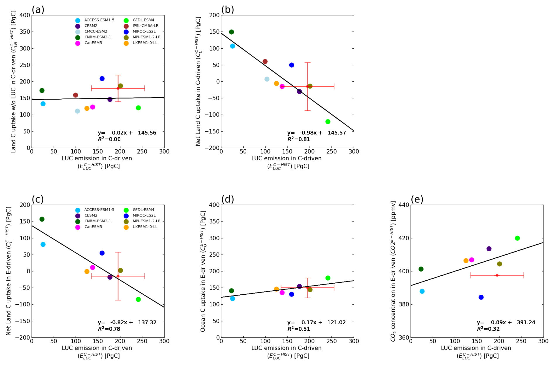
Figure 8 Relationships of cumulative land use change emission diagnosed from concentration-driven historical experiments ($E_{\mathrm{LUC}}^{\text{C-HIST}}$) with other variables. The upper panels represent $E_{\mathrm{LUC}}^{\text{C-HIST}}$ versus (a) cumulative land carbon uptake without a consideration of land use change ($C_{\mathrm{LN}}^{\text{C-HIST}}$, which is identical to $C_{\mathrm{L}}^{\text{C-HIST-NOLU}}$) and (b) cumulative net land carbon uptake ($C_{\mathrm{L}}^{\text{C-HIST}}$) in concentration-driven historical experiments. The lower panels are scatterplots for emission-driven historical experiments, presenting $E_{\mathrm{LUC}}^{\text{C-HIST}}$ versus (c) cumulative net land carbon uptake ($C_{\mathrm{L}}^{\text{E-HIST}}$), (d) cumulative ocean carbon uptake ($C_{\mathrm{O}}^{\text{E-HIST}}$), and (e) simulated CO₂ concentration (CO2^E-HIST). The numbers of analyzed models differ between the concentration-driven (upper panels) and emission-driven (lower panels) experiments because of data availability. Red bars represent the range of uncertainty obtained from GCB2021 (Friedlingstein et al., 2021).

4.2 Growth of atmospheric CO₂ in five qualitatively divided eras

The analyses so far have used cumulative values of the carbon fluxes at the end of the historical simulation, and, thus, it is difficult to specify the period in which the biases of simulated CO₂ concentration and/or carbon fluxes arise. Here, we propose a method that helps to identify the period using simulated CO₂ concentrations.

First, we compared the simulated CO₂ concentrations of E-HIST and the prescribed concentration used in C-HIST (Fig. 9); the absolute concentration is shown in Fig. 9a, and the annual CO₂ growth rate is shown in Fig. 9b. As shown in Fig. 3, the multi-model mean of the CO₂ concentration agreed well with the concentration pathways of the reference data, except for the period of 1940–1960, during which the atmospheric growth rate in the reference data remained almost zero.

Second, we divided the historical period of 1850–2014 into five eras based on qualitative characteristics, and then the cumulative CO₂ growth in each era was evaluated (Fig. 9c). The definitions of the five eras are follows:

• Era 1 (1850–1899). This is the period corresponding to preindustrial conditions; land use change emission is the dominant source of anthropogenic CO₂ emission.

• Era 2 (1900–1939). This is the period after the start of the industrial revolution, in which fossil fuel emission becomes comparable with land use change emission.

• Era 3 (1940–1959). This is the period when the observed CO₂ concentration determined from ice core measurement suggests a concentration plateau.

• Era 4 (1960–1999). This is the period when the direct measurement of atmospheric CO₂ started, during which fossil fuels become the dominant source of anthropogenic emission, and agriculture (cropland expansion and application of nitrogen fertilizer) rapidly grows; nitrogen deposition increases are accompanied by worsening air quality.

• Era 5 (2000–2014). This is the recent period before the Paris Agreement, during which the growth of fossil fuel emission continues. More observation datasets, including satellite measurements, become available for evaluating carbon cycle processes in models. Nitrogen deposition is reduced because of air pollution regulations.

In Fig. 9d, the simulated concentration bias at the end of each era was visualized by normalizing the concentration bias as follows:

$$\begin{array}{}\text{(4)}& \begin{array}{rl}\mathrm{NB}\left(i,j\right)& ={\displaystyle \frac{\mathrm{\Delta }\mathrm{CO}\mathrm{2}\left(i,j\right)-\mathrm{\Delta }{\mathrm{CO}\mathrm{2}}^{\mathrm{CMIP}\mathrm{6}\mathrm{F}}\left(i\right)}{\mathrm{\Delta }{\mathrm{CO}\mathrm{2}}^{\mathrm{CMIP}\mathrm{6}\mathrm{F}}\left(i\right)}};\\ i& =\mathrm{1},\mathrm{\dots },\mathrm{5};j=\mathrm{1},\mathrm{\dots },\mathrm{12},\end{array}\end{array}$$

where NB(i,j) represents the normalized bias at the end of each era (i=1 to 5) in each model (j=1 to 12), and ΔCO2(i)^CMIP6F and ΔCO2(i,j) are the change in CO₂ concentration in the reference data and the change in the simulated concentration, respectively.

In era 1, half the models underestimate the CO₂ concentration by a few parts per million by volume at the end of this period, while other models reproduce the CO₂ concentration well (except EC-Earth-CC and CNRM-ESM2-1, which overestimate the concentration). In this era, land use change is the dominant source of anthropogenic emission; therefore, the simulated CO₂ concentration bias is most likely caused by biases in land use change processes in the models. Era 2 represents the period after the start of the industrial revolution, but land use change emissions continued to increase. Most models with a positive (negative) concentration bias in era 2 have a positive (negative) concentration bias in era 1 as well.

At the end of era 3, all models overestimate the CO₂ concentration by approximately 5 ppmv on average. The possible reasons for such overestimation are numerous: (1) the CO₂ emission used for E-HIST might be larger than that expected from the observed CO₂ concentration. The Law Dome ice core record (Etheridge et al., 1996) used for historical CO₂ concentrations shows almost no increase during the 1940s (< 1.5 ppm), which is inconsistent with the 14 PgC emissions during this decade. (2) The ocean and/or land might have strengthened carbon sinks during this period, attributable to internal climate variability (Joos et al., 1999), which cannot be captured by the freely evolving climate simulations. (3) The land use change emissions simulated by the ESMs for this period are perhaps larger than observed because the land abandonment during World War II might have led to reduced CO₂ emissions from land use change (Bastos et al., 2016).

In eras 4 and 5, various processes such as land use change, agriculture, and nitrogen deposition, as well as carbon cycle feedbacks, become increasingly important. However, the normalized concentration bias shown in Fig. 9d is smaller than that in the other periods, likely because land use change emission in eras 4 and 5, which is the most uncertain term of the global carbon budget, becomes weaker in this period. More than six models reproduce the positive CO₂ biases in eras 4 and 5, while the other models largely underestimate the rate of growth in the CO₂ concentration.

Here, we demonstrate that the division of the historical period into the five eras and the assessment of CO₂ growth can link the dynamics of global carbon cycle processes that work behind the concentration evolution. The assessment of CO₂ over the individual eras is essentially the same as that found in the examination of the annual growth rate of CO₂ shown in Fig. 9b. However, this method has three advantages over the comparison of the annual CO₂ growth rate: (1) the discrepancies among the models are emphasized and clearly visualized; (2) the sum of the concentration biases in each era is identical to the concentration bias at the end of the historical experiment, which makes it easy to find linkages between the concentration bias over the entire simulation period and in each of the divided periods; and (3) the qualitatively characterized period can draw the attention of modelers to the dominant processes specific to each period, suggesting that the consideration of such processes should be improved. Further analysis that combines this method (Fig. 9) with the feedback analysis (Table 5) would be helpful when identifying quantitatively the mechanism of CO₂ concentration changes in each era (Fig. S7).

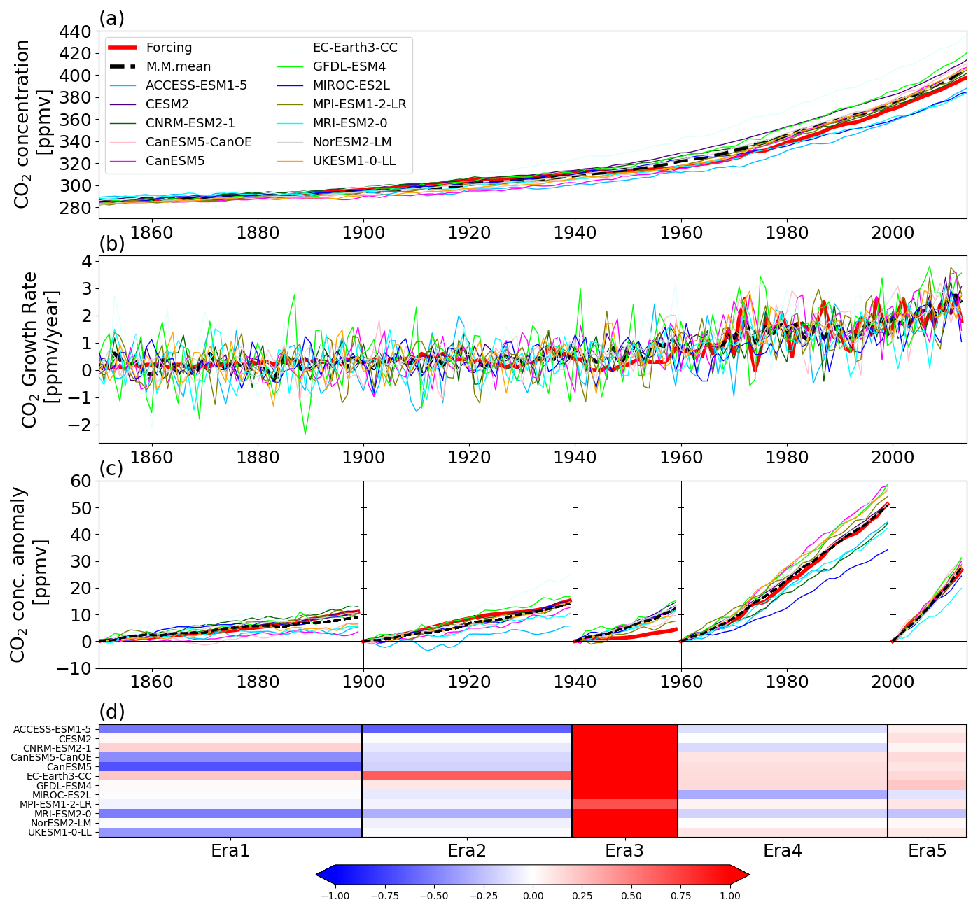
Figure 9 Temporal variation in global CO₂ concentration simulated by the CMIP6 ESMs (CO2^E-HIST) and the analysis: (a) annual mean CO₂ concentration, (b) annual CO₂ growth rate, (c) CO₂ concentration anomaly in five eras, and (d) normalized bias in each era. In (a) and (b), the thick red line represents the CO₂ concentration used as prescribed data for CMIP6, the CO₂ concentration simulated by each model is represented by the thin colored lines, and the multi-model mean (12 ESMs) is shown by the thick dashed line. In (c), the historical period is divided into five eras, and the CO₂ concentration anomaly from the beginning of each era (1850, 1900, 1940, 1960, and 2000) is presented. The heatmap in (d) shows the normalized CO₂ concentration bias in each era, with a stronger positive (negative) bias shown by the denser red (blue) color. The calculation of normalized concentration bias follows Eq. (5).

5 Summary and conclusions

In this study, with the objective of acquiring insights into how to improve the accuracy of atmospheric CO₂ concentrations simulated by ESMs, we examined both C-driven and E-driven types of simulations by CMIP6 ESMs. Generally, E-driven historical experiments have advantages in terms of capturing the causal chains of climate–carbon processes as they occur in the real world and are expected to evaluate the full span of the uncertainty range that covers the entire carbon–climate system. Meanwhile, C-driven historical simulations can isolate and evaluate the forced responses and feedback processes of the Earth system, particularly the carbon cycle processes. We first examined the consistency between C- and E-driven simulations with regard to the fundamental terms of the global carbon budgets (fossil fuel and land use change emissions, land and ocean carbon uptakes, and atmospheric CO₂ concentration; Fig. 1). The multi-model means of the two types of experiment generally show good agreement with each other (Fig. 3 and Table 4), but some discrepancies were found. The cumulative compatible fossil fuel emission diagnosed from C-driven experiments is lower by approximately 35 PgC than the prescribed emission used to drive the E-driven historical experiment. The simulated CO₂ concentration at the end of the E-driven historical simulation is higher than that of the observed value by 7 ppmv. Although the reason for these discrepancies between the C-driven and E-driven historical experiments is unclear, the overestimation of simulated CO₂ concentration is sufficiently small to make the multi-model averages of GSAT between the E-driven and C-driven simulations negligible. The spread of GSAT among the models, however, was found to become larger in the E-driven experiment (± 0.37 °C) than in the C-driven experiment (± 0.28 °C) because of the large variation in the simulated CO₂ concentrations (± 14 ppmv), suggesting that the E-driven setting would bring additional uncertainty into the simulated GSAT owing to the bias in the simulated CO₂ concentration. This small additional spread in historical simulations is compensated for by the advantage of being able to span the uncertainty in future projections much more fully.

The magnitude of simulated net land carbon uptake is determined by the strength of terrestrial carbon cycle feedbacks and the response to land use change forcing. Although the multi-model spread of the net land carbon uptake C_L is large (6.0 ± 74.2 PgC for the C-driven experiments and 15.2 ± 65.5 PgC for the E-driven experiments; Table 4), the relative order between the models was almost unchanged between the C-driven and E-driven experiments (R²=0.97, Fig. 4a). In contrast, some individual models showed a distinctly different magnitude of ocean carbon uptake between the C-driven and E-driven experiments (R²=0.01, Fig. 4b). A likely reason is that the E-driven setting allows ocean carbon fluxes to be dependent on land carbon fluxes via CO₂–carbon feedback, and, thus, a portion of the bias in the land carbon flux is imposed on the ocean flux. In particular, land use change emission, which is a component flux of the net atmosphere–land carbon exchange, is not a feedback process but a forced response to land use change. Thus, the bias in land use change emission is likely to be imposed on the ocean carbon flux in the E-driven simulations. This mechanism explains the fact that the magnitude of the ocean carbon sink in the E-driven setting is more correlated with land carbon uptake (R²=0.56, Fig. 4d) rather than with the magnitude of the ocean carbon sink that is evaluated in the C-driven historical simulation (Fig. 4b). Additionally, the interlinking mechanism between land and ocean can partly offset the carbon flux bias found in one component by imposing it onto the other, which sometimes makes the trajectory of atmospheric CO₂ concentration in E-driven simulations more realistic.

The magnitudes of the natural carbon sinks of land and ocean are affected by carbon cycle feedback processes, which have been widely evaluated using idealized experimental settings (e.g., Arora et al., 2020). In this study, the linkages of land and ocean carbon sinks between the idealized experiment (C-1PCT) and the C-driven historical experiment (C-HIST) were investigated (Fig. 7). We found that the magnitudes of the ocean carbon sink in the historical simulation were well explained by those evaluated in C-1PCT, likely because of the dominant role of CO₂–carbon feedback in determining the magnitude of the ocean carbon sink. Meanwhile, the magnitudes of land carbon uptake showed a weak linkage between C-1PCT and the C-driven historical run, where land use and land cover are fixed (C-HIST-NOLU), despite the absence of land use change impacts in both experiments. Further detailed analysis suggested that the non-CO₂ effects (i.e., climate–carbon feedback induced by non-CO₂ agents and direct stimulation of land biogeochemistry via nutrient input) could play a role in causing the large difference in the natural carbon sink between the two experiments (Table 5 and Appendix C). However, this conclusion was based on simulations by two models, and, thus, to obtain a more robust conclusion, it will be necessary for larger numbers of models to participate in all the experiments listed in Table 2. Particularly, the DAMIP hist-CO2 experiment was performed by only two ESMs, thereby precluding all others from the more detailed analysis.

These quantitative assessments between C- and E-driven historical experiments were confirmed by multiple CMIP6 ESMs, and one of the most important confirmations obtained from this study was the fact that a strong negative correlation was found between the simulated CO₂ concentration and the compatible fossil fuel emission (R²=0.91, Fig. 5b). This suggests that reasonable reproduction of compatible fossil fuel emission in the C-driven experiments likely assures reasonable performance of the simulated CO₂ concentration in the E-driven experiments, although most of the current generation of ESMs analyzed in this study cannot reproduce the compatible fossil fuel emission reasonably, i.e., within the range of GCB2021. In CMIP6, the multi-model average values of $E_{\mathrm{FF}}^{\text{C-HIST}}$ and CO2^E-HIST are 374 PgC and 405 ppmv, respectively, whereas the corresponding GCB2021 values are 400 ± 20 PgC and 397.6 ppmv, respectively. The visualization of each model status regarding the global carbon budget and showing the gap in relation to GCB2021 on the plotting space of $E_{\mathrm{FF}}^{\text{C-HIST}}$ vs. CO2^E-HIST (Fig. S6) might provide further guidance with regard to the best means to improve the global carbon budget in both C- and E-driven historical simulations.

In this study, much of the discussion concerned comparisons with GCB2021, which is regarded to be the best aggregation of scientific knowledge with regard to the global carbon budget (e.g., Table 4 and Fig. 3). Through such comparisons, it is suggested that the natural land sink simulated by ESMs (148 ± 31 PgC, C_LN in Table 4) is lower than that of GCB2021 (180 ± 40 PgC), which relies on offline land and ocean biogeochemistry models. In addition to the global-scale discrepancy, it has already been identified that the CMIP6 multi-model mean performed well for all regions and variables assessed by the RECCAP2 regional assessments for the land carbon cycle; however, no single model performed well for every region or for every variable, and there were complex signals with regard to the role of process inclusion in helping improve model fidelity (Jones et al., 2023). In this study, it was also confirmed that ESMs generally simulate smaller cumulative land use change emission (129 ± 67 PgC) than that reported by GCB2021 (195 ± 60 PgC); the estimation spreads in both GCB2021 and ESMs are the largest among the basic components of the global carbon budget (CO₂, C_O, C_LN, and E_LUC in Table 4). The overall methodology for estimating land use change emission is different between GCB2021 and ESMs (bookkeeping method versus process-based estimation) and in the details of the emission calculations and assumptions (e.g., ESMs diagnose the emission by taking the anomaly between two different historical experiments, whereas GCB methods usually assume constant land biomass throughout the historical period). Therefore, the mechanism that produces such systematic discrepancies between the GCB models and ESMs, particularly the processes that control the magnitude of land use change emission, should be explored intensively in future work.

To help identify the period when the biases of simulated CO₂ concentration and/or carbon fluxes arise, this study proposed a method to evaluate the growth of simulated CO₂ concentrations in five eras that were characterized qualitatively (Fig. 9). The division succeeded in clarifying the period during which the CO₂ concentration biases of the models are produced and, thus, could draw the attention of modelers to the most important processes specific to each period. One common feature confirmed among the models was the overestimation of CO₂ concentration during the 1940–1959 period, when ice core measurements suggest a CO₂ concentration plateau. Although it is difficult to specify the reason based on this study, the models produce an overestimation of approximately 5 ppmv on average in this era. Furthermore, the results suggested the causes of the CO₂ concentration bias: e.g., models that underestimated the CO₂ concentration in 1850–1899 likely simulate relatively low land use change emission in this period. Such suggestions would be validated in future work that extends the analysis to include feedback analysis (Fig. S7). Additionally, extension of the historical simulation beyond 2020 and consideration of an additional analysis with one more era following the Paris Agreement might help to highlight implications for global warming mitigation policies.

Finally, on the basis of the findings of this study, suggestions to improve the CO₂ concentration simulated by ESMs are summarized as follows:

1. It is likely that a model with a cumulative compatible fossil fuel emission of approximately 400 PgC during 1850–2014 would be able to adequately capture the CO₂ concentration level in the E-driven historical experiment. A model with a larger compatible fossil fuel emission in a C-driven run should have a lower simulated CO₂ concentration in an E-driven experiment and vice versa. However, most CMIP6 ESMs cannot simulate compatible fossil fuel emission within the range of the GCB2021 estimate; consequently, they cannot reproduce an accurate CO₂ concentration at the end of the historical simulation.

2. To accurately reproduce the atmospheric CO₂ concentration, simulating land and ocean carbon uptakes with reasonable magnitudes is necessary. We should recognize that these carbon uptakes in a model can behave differently among various types of simulations. The magnitude of ocean carbon uptakes simulated in the 1 % CO₂ experiment explains that in the C-driven historical simulations well, likely because of the dominant role of CO₂–carbon feedback in the ocean; however, the ocean sink in the C-driven historical simulation can be different from that in the E-driven simulation, in which carbon uptakes by the land and the ocean interact via CO₂ concentration, and, thus, a portion of carbon flux bias on land can be imposed on the ocean carbon flux. Meanwhile, land carbon uptakes between the C- and E-driven historical simulations behave very similarly; however, it is difficult to approximate the magnitude of land carbon uptakes in the historical simulations from the simulation result of the idealized experiment because land carbon uptake probably experiences non-negligible impacts as a result of non-CO₂ effects (climate–carbon feedback induced by non-CO₂ agents and/or direct stimulation of land carbon uptake via nutrient inputs) that are absent in the idealized experiment.

3. One of the largest estimation spreads among the models was found in the term of land use change emission, and accurate reproduction of land use change emission is critical for better reproduction of CO₂ concentration and other global carbon budget terms. The magnitude of simulated land use change emission not only affects the level of net land carbon uptake but also determines the magnitude of the ocean carbon sink in the E-driven experiment. In the current generation of ESMs, the ocean carbon sink in the E-driven experiment is well explained by the magnitude of the simulated land use emissions rather than by the magnitude of the ocean carbon sink that is evaluated in the C-driven historical experiment. For CMIP7 and beyond, performing hist-noLu experiments with more models in both the historical and future periods would allow for a more accurate quantification of the simulated land use change emissions and for clarification of the reasons for such variations in the land use change emission in ESMs and the large discrepancy between ESMs and GCB models.

4. Ideas for improved model performance in terms of the global carbon budget would be inspired through evaluation of the simulated CO₂ concentration in emission-driven historical experiments because CO₂ concentration is observed or estimated with the lowest estimation uncertainty. An analysis that divides the entire historical simulation period into five eras would be helpful to specify when the concentration bias is produced in the models. Future work that includes further feedback analysis in the five eras will enable identification of the mechanism behind the CO₂ concentration bias.

Appendix A: Derivation of the global carbon budget equations in flux and cumulative values

The global carbon budget equation can be formalized using global carbon flux variables as follows:

$$F_{\mathrm{FF}}\left(t\right)={\displaystyle \frac{\mathrm{d}{C}_{\mathrm{A}}^{\prime }\left(t\right)}{\mathrm{d}t}}+\mathrm{fgco}\mathrm{2}\left(t\right)+\mathrm{nbp}\left(t\right),$$

where F_FF(t) is the carbon flux of fossil fuel emission; fgco2(t) and nbp(t) are the net atmosphere–ocean and atmosphere–land carbon fluxes, respectively; and $C_{\mathrm{A}}^{\prime }\left(t\right)$ is the amount of carbon in the atmosphere.

By integrating both sides of the equation with time t, we obtain the following:

$$\int F_{\mathrm{FF}}\left(t\right)\mathrm{d}t=\mathrm{\Delta }{C}_{\mathrm{A}}^{\prime }\left(t\right)+\int \mathrm{fgco}\mathrm{2}\left(t\right)\mathrm{d}t+\int \mathrm{nbp}\left(t\right)\mathrm{d}t,$$

with this equation being equivalent to

$$E_{\mathrm{FF}}\left(t\right)=\mathrm{\Delta }{C}_{\mathrm{A}}^{\prime }\left(t\right)+\mathrm{\Delta }{C}_{\mathrm{O}}^{\prime }\left(t\right)+\mathrm{\Delta }{C}_{\mathrm{L}}^{\prime }\left(t\right),$$

where $E_{\mathrm{FF}}\left(t\right)=\int F_{\mathrm{FF}}\left(t\right)\mathrm{d}t$, $\mathrm{\Delta }{C}_{\mathrm{O}}^{\prime }\left(t\right)=\int \mathrm{fgco}\mathrm{2}\left(t\right)\mathrm{d}t$, and $\mathrm{\Delta }{C}_{\mathrm{L}}^{\prime }\left(t\right)=\int \mathrm{nbp}\left(t\right)\mathrm{d}t$.

By further replacing $\mathrm{\Delta }{C}_{\mathrm{A}}^{\prime }\left(t\right)$ with C_A, $\mathrm{\Delta }{C}_{\mathrm{O}}^{\prime }\left(t\right)$ with C_O, and $\mathrm{\Delta }{C}_{\mathrm{L}}^{\prime }\left(t\right)$ with C_L, this equation can be expressed as follows:

$$\begin{array}{}\text{(A1)}& E_{\mathrm{FF}}=C_{\mathrm{A}}+C_{\mathrm{O}}+C_{\mathrm{L}}.\end{array}$$

This is the same as Eq. (1b).

Appendix B: Compatible fossil fuel emission modified by residual sink or source terms

With regard to Eq. (A1), we assumed in this study that C_O and C_L for 2014 correspond to the cumulative land–atmosphere and ocean–atmosphere CO₂ exchange, respectively, during 1850–2014; i.e., $C_{\mathrm{L}}={\int }_{\mathrm{1850}}^{\mathrm{2014}}\mathrm{nbp}\mathrm{d}t$ and $C_{\mathrm{O}}={\int }_{\mathrm{1850}}^{\mathrm{2014}}\mathrm{fgco}\mathrm{2}\mathrm{d}t$. However, this assumption does not always hold strictly in the ESM simulations for the following reasons:

1. Models might have an additional source or sink of carbon attributable to external natural carbon inputs or losses (IB_natural), which is not represented in Eq. (A1), e.g., natural carbon input by volcanic eruptions (Hajima et al., 2020) or a “missing carbon sink” to partly offset the external carbon input from rivers (Séférian et al., 2019).

2. Models sometimes have an additional source or sink of carbon that arises from imperfect mass conservation in advection schemes or other artifacts in models (IB_artifact).

By explicitly expressing these additional sink or source terms, Eq. A1 can be expressed as follows:

$$\begin{array}{}\text{(B1)}& E_{\mathrm{FF}}=C_{\mathrm{A}}+C_{\mathrm{O}}+C_{\mathrm{L}}+\text{IB},\end{array}$$

where IB = IB_natural+ IB_artifact.

The IB in each model can be assessed by applying the E-HIST result to Eq. (B1) as follows:

$$\begin{array}{c}{\displaystyle }{\text{IB}}^{\text{E-HIST}}\\ {\displaystyle }=E_{\mathrm{FF}}^{CMIP\mathrm{6}}-C_{\mathrm{A}}^{\text{E-HIST}}-C_{\mathrm{O}}^{\text{E-HIST}}-C_{\mathrm{L}}^{\text{E-HIST}}\\ {\displaystyle }=E_{\mathrm{FF}}^{\mathrm{CMIP}\mathrm{6}}-C_{\mathrm{A}}^{\text{E-HIST}}-{\int }_{\mathrm{1850}}^{\mathrm{2014}}\mathrm{fgco}{\mathrm{2}}^{\text{E-HIST}}\mathrm{d}t\\ {\displaystyle }-{\int }_{\mathrm{1850}}^{\mathrm{2014}}{\mathrm{nbp}}^{\text{E-HIST}}\mathrm{d}t,\end{array}$$

where $E_{\mathrm{FF}}^{\mathrm{CMIP}\mathrm{6}}$ is the cumulative value of the emission applied to E-HIST, and the other three terms are obtained from the E-HIST simulation by each model.

We note that the atmospheric CO₂ concentrations in E-HIST were simulated under the influence of those additional source or sink terms, while the compatible fossil fuel emission was not. Thus, the compatible fossil fuel emission obtained from C-HIST should also reflect those additional source or sink terms in the calculation, particularly when investigating potential linkages between E-HIST and C-HIST. The compatible fossil fuel emission modified by the residual sink or source terms can be written as follows:

$$\begin{array}{c}{\displaystyle }{E}_{\mathrm{FF}}^{\text{C-HIST}}=C_{\mathrm{A}}^{\mathrm{CMIP}\mathrm{6}}+{\int }_{\mathrm{1850}}^{\mathrm{2014}}\mathrm{fgco}{\mathrm{2}}^{\text{C-HIST}}\mathrm{d}t\\ {\displaystyle }+{\int }_{\mathrm{1850}}^{\mathrm{2014}}{\mathrm{nbp}}^{\text{C-HIST}}\mathrm{d}t+{\mathrm{IB}}^{\text{C-HIST}}\\ {\displaystyle }=C_{\mathrm{A}}^{\mathrm{CMIP}\mathrm{6}}+{\int }_{\mathrm{1850}}^{\mathrm{2014}}\mathrm{fgco}{\mathrm{2}}^{\text{C-HIST}}\mathrm{d}t\\ {\displaystyle }+{\int }_{\mathrm{1850}}^{\mathrm{2014}}{\mathrm{nbp}}^{\text{C-HIST}}\mathrm{d}t+{\mathrm{IB}}^{\text{E-HIST}},\end{array}$$

assuming IB^C-HIST= IB^E-HIST.

Appendix C: Carbon changes expressed by four types of drivers and their assessment

Table C1 Same as Table 1 but extended to include the combinations of experiments used to evaluate $C_{X<\text{CO2-BGC}>}$, $C_{X<\text{CO2-CLIM}>}$, $C_{X<\text{LUC}>}$, and $C_{X<\text{NONCO2}>}$.

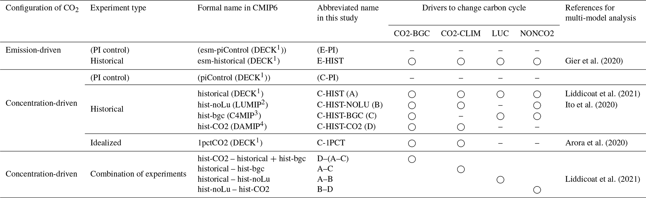
Here, we assume that cumulative land or ocean carbon uptake C_X (X denotes L or O) can be presented as the sum of the carbon changes caused by four types of drivers:

$$\begin{array}{}\text{(C1)}& \begin{array}{rl}{C}_X& =C_{X<\text{CO2-BGC}>}+C_{X<\text{CO2-CLIM}>}\\ & +C_{X<\text{LUC}>}+C_{X<\text{NONCO2}>},\end{array}\end{array}$$

where

1. $C_{X<\text{CO2-BGC}>}$ is the carbon change induced by CO₂–carbon feedback (CO2-BGC);

2. $C_{X<\text{CO2-CLIM}>}$ is the carbon change caused by CO₂-induced warming and the resultant climate–carbon feedback (CO2-CLIM);

3. $C_{X<\text{LUC}>}$ is the carbon change induced by land use change (LUC);

4. $C_{X<\text{NONCO2}>}$ is the carbon change induced by non-CO₂ effects (NONCO2), including warming or cooling effects of non-GHG agents and direct stimulation of biogeochemistry via external nutrient inputs.

Here, to separately evaluate the drivers of $C_{X<\text{CO2-BGC}>}$, $C_{X<\text{CO2-CLIM}>}$, $C_{X<\text{LUC}>}$, and $C_{X<\text{NONCO2}>}$, we used four types of historical experiments with the C-driven setting (C-HIST, C-HIST-NOLU, C-HIST-BGC, and C-HIST-CO2; Table 1). These experiments were originally designed to evaluate the forced responses and feedback processes of the climate system. On the basis of experimental protocols, C_X in each simulation can be expressed as outlined below (see also Table C1).

C-HIST.

$$\begin{array}{}\text{(C2)}& \begin{array}{rl}{C}_X^{\text{C-HIST}}& =C_{X<\text{CO2-BGC}>}^{\text{C-HIST}}+C_{X<\text{CO2-CLIM}>}^{\text{C-HIST}}\\ & +C_{X<\text{LUC}>}^{\text{C-HIST}}+C_{X<\text{NONCO2}>}^{\text{C-HIST}}\end{array}\end{array}$$

C-HIST-NOLU.

$$\begin{array}{}\text{(C3)}& \begin{array}{rl}{C}_X^{\text{C-HIST-NOLU}}& =C_{X<\text{CO2-BGC}>}^{\text{C-HIST}}+C_{X<\text{CO2-CLIM}>}^{\text{C-HIST}}\\ & +C_{X<\text{NONCO2}>}^{\text{C-HIST}}\end{array}\end{array}$$

This is because prescribed land use and land cover changes are fixed at the preindustrial level, making the terrestrial $C_{X<\text{LUC}>}^{\text{C-HIST}}$ zero (Lawrence et al., 2016).

C-HIST-BGC.

$$\begin{array}{}\text{(C4)}& \begin{array}{rl}{C}_X^{\text{C-HIST-BGC}}& =C_{X<\text{CO2-BGC}>}^{\text{C-HIST}}+C_{X<\text{LUC}>}^{\text{C-HIST}}\\ & +C_{X<\text{NONCO2}>}^{\text{C-HIST}}\end{array}\end{array}$$

This is because climate–carbon feedback is suppressed in this experiment, and, thus, $C_{X<\text{CO2-CLIM}>}^{\text{C-HIST}}$ can be assumed to be zero (Jones et al., 2016).

C-HIST-CO2.

$$\begin{array}{}\text{(C5)}& C_X^{\text{C-HIST-CO2}}=C_{X<\text{CO2-BGC}>}^{\text{C-HIST}}+C_{X<\text{CO2-CLIM}>}^{\text{C-HIST}}\end{array}$$

This is because external forcings other than CO₂ (i.e., non-CO₂ GHG concentrations, aerosol emissions, land use change, and nitrogen deposition) are fixed at their preindustrial levels, and the change in atmospheric CO₂ concentration is the only driver of anthropogenic change in the climate system (Gillett et al., 2016).

From the four types of historical experiments, we can separately assess $C_{X<\text{CO2-BGC}>}$, $C_{X<\text{CO2-CLIM}>}$, $C_{X<\text{LUC}>}$, and $C_{X<\text{NONCO2}>}$ using Eqs. (C2)–(C5) as follows (see also Table C1):

$$\begin{array}{c}{\displaystyle }{C}_X^{\text{C-HIST}}-C_X^{\text{C-HIST-NOLU}}=C_{X<\text{LUC}>},\\ {\displaystyle }{C}_X^{\text{C-HIST}}-C_X^{\text{C-HIST-BGC}}=C_{X<\text{CO2-CLIM}>},\\ {\displaystyle }{C}_X^{\text{C-HIST-BGC}}-C_X^{\text{C-HIST-CO2}}=C_{X<\text{NONCO2}>},\\ {\displaystyle }{C}_X^{\text{C-HIST-CO2}}-(C_X^{\text{C-HIST}}-C_X^{\text{C-HIST-BGC}})=C_{X<\text{CO2-BGC}>}.\end{array}$$

We note that nonlinear terms (i.e., interactive effects between $C_{X<\text{CO2-BGC}>}$, $C_{X<\text{CO2-CLIM}>}$, $C_{X<\text{LUC}>}$, and $C_{X<\text{NONCO2}>}$) are assumed to be zero.