Technical note: A modified formulation of dynamic energy budget theory for faster computation of biological growth

The mass conservation equation in the presence of boundary fluxes and chemical reactions from non-equilibrium thermodynamics is used to derive a modified dynamic energy budget (mDEB) model. Compared to the standard dynamic energy budget (sDEB) model (Kooijman, 2009), this modified formulation does not place the dilution effect in the mobilization kinetics of reserve biomass, and it maintains the partition principle for reserve mobilization dynamics for both linear and non-linear kinetics. Overall, the mDEB model shares most features with the sDEB model. However, for biological growth that requires multiple nutrients, the mDEB model is computationally much more efficient by not requiring numerical iterations for obtaining the specific growth rate. In an example of modeling the growth of Thalassiosira weissflogii in a nitrogen-limiting chemostat, the mDEB model was found to have almost the same accuracy as the sDEB model while requiring almost half of the computing time of the sDEB model. Since the sDEB model has been successfully applied in numerous studies, we believe that the mDEB model can help improve the modeling of biological growth and the associated ecosystem processes in various contexts.

1 Introduction

By aid of membranes (and cell walls), biological cells create an intracellular environment where substrates taken up from the environment are concentrated and converted into new biomass and new cells (Lodish et al., 1999). The similarity between the role played by the (membrane-confined) intracellular environment and the (container-held) aqueous solution that supports chemical reaction experiments (in the lab) has motivated the development of variable-internal-store models to model biological growth (Nev and Van Den Berg, 2017; Grover, 1991; Droop, 1974; Williams, 1967). Among the many formulations, the dynamic energy budget (DEB) model has been a very successful example (Kooijman, 2009; Tolla et al., 2007; Sousa et al., 2010; Matyja and Lech, 2024; Tang and Riley, 2015).

The key idea of variable-internal-store models is to represent a biological organism with one structural compartment, which holds one or multiple storage compartments (Nev and Van Den Berg, 2017; Kooijman, 2009). The production of new cells is modeled as the growth of structural biomass, as driven by the transformation dynamics of storage compartments. These models vary in their formulation of storage dynamics and how the turnover of storage drives structural growth. In the DEB framework, storage is termed “reserve”, whereas in the Droop model, storage is termed “quota”. Since here we are proposing a modified DEB model (mDEB), we use the term “reserve” hereafter. Moreover, in Dynamic Energy Budget Theory for Metabolic Organisation (Kooijman, 2009), we note that standard DEB model refers to the simplest non-degenerated DEB model. In this study, we use the standard dynamic energy budget (sDEB) model simply to semantically contrast the formulation in Kooijman (2009) with the mDEB proposed here.

The sDEB model adopts the following three key assumptions:

1. The strong homeostasis assumption is abstracted from observations that almost every biological organism is made up of several groups of macromolecules, e.g., carbohydrates, proteins, lipids, and nucleic acids (Lodish et al., 1999). This assumption states that the chemical composition of reserve(s) and structure(s) is constant, but their amounts can vary.

2. The weak homeostasis is abstracted from observed stable whole-organism elemental stoichiometry, such as the Redfield ratio (Redfield, 1934), which is the foundation for the application of ecological stoichiometry theory (Sterner and Elser, 2002). This assumption states that if food density does not change, then reserve density, defined as the ratio between the amounts of reserve and structure, becomes constant while growth continues. That is, reserve and structure grow in harmony, and the chemical composition of biomass does not change.

3. The principle of merging and partitioning of reserves is abstracted from the evolution from unicellular to multicellular life forms.

These assumptions combined with Euler's theorem on homogeneous function are used to infer that the reserve turnover dynamics must be a linear function of reserve density (see Chap. 2 of Kooijman (2009) for details).

Recently, Tang and Riley (2023) suggested that the linear reserve dynamics in the sDEB model can be replaced with more generic nonlinear enzyme kinetics (derived from law of mass action) without violating the principle of merging and partitioning of reserves so that a closer link can be built between the DEB model and models that consider intracellular biochemistry using explicit enzyme kinetics (Etienne et al., 2020; Tadmor and Tlusty, 2008). Tang and Riley (2023) demonstrated that their revised DEB (rDEB) model outperformed the sDEB model for a measured time series of degradation of the herbicide 2,4-dichlorophenoxyacetic acid, and both DEB models resulted in a better explanation than the popular compromise model for the empirically observed relationships (1) between specific respiration and specific growth rate for the marine bacterial data collected by Vikström and Wikner (2019) and (2) between specific substrate uptake rate and biomass yield for the microbial data synthesis by Smeaton and Van Cappellen (2018). However, in further exploration of the rDEB model, Tang and Riley (2023) noticed (in their Sect. 4.2) that the sDEB model is paradoxically recovered from the rDEB only when the ribosome effort allocated to growth is zero. Thus, in the following, we derive the reserve dynamics using an alternative approach that combines the first law of thermodynamics and law of mass action, which then leads to the mDEB model. As we show below, the mDEB model remains compatible with all key assumptions of the sDEB model and can be easily extended to a non-linear enzyme-kinetics-based model of intracellular metabolism. Moreover, the mDEB model extension to multiple-substrate-limited biological growth is computationally much more efficient while maintaining the theoretical elegance of the DEB theory. We note that this gained computational efficiency by the mDEB model will be very helpful to apply the DEB theory to the modeling of a large number of concurrently growing organisms (or organs for plants and animals).

Below we first provide a detailed derivation of the mDEB model. Then the mDEB model is compared to the sDEB model for general behaviors. Following this, an application to the chemostat experiment by Pawlowski (2004) is presented. Finally, we conclude by discussing how the mDEB model can be applied to growth problems in ecosystem biogeochemistry.

2 Theory

2.1 The mDEB model

We start with the mass conservation equation from the non-equilibrium thermodynamics (De Groot and Mazur, 1984):

$$\begin{array}{}\text{(1)}& {\displaystyle \frac{\mathrm{d}}{\mathrm{d}t}}{\int }_{V\left(t\right)}{\mathit{\rho }}_i\mathrm{d}V=-{\int }_{\mathbf{\Omega }\left(t\right)}{\mathit{J}}_i\cdot \mathrm{d}\mathbf{\Omega }+{\int }_{V\left(t\right)}{\sum }_l{\mathit{\sigma }}_{li}{r}_l\left({\mathit{\rho }}_l\right)\mathrm{d}V,\end{array}$$

where subscript i refers to pools internal to the time-dependent volume V(t); ρ_i is the mass (or energy) density of the ith internal pool that is enclosed by the volume V(t), whose surface is Ω(t); J_i is the outgoing flux of ρ_i through the surface Ω(t); and r_l(ρ_l) is the lth chemical reaction rate that occurs inside the volume V(t) contributing to the change of total mass ∫_V(t)ρ_idV according to the stoichiometric parameter σ_li. In plain language, Eq. (1) states that the changing rate of total mass ∫_V(t)ρ_idV within a volume of space V(t) (i.e., left-hand side) is determined by the mass flux escaping through its surface Ω(t) (i.e., the first term on the right-hand side) and the net chemical production inside the volume (the second term in the right-hand side). We define all the symbols in the nomenclature table in the Appendix, and unless specified otherwise, all variables have ISO units.

When applied to a biological cell, V(t) is its physical volume, and Ω(t) is the corresponding exterior surface. The ith internal reserve is ρ_i, whose dynamics are governed by substrate uptake (−J_i) and intracellular chemical transformations (by the last term of Eq. 1). Since Eq. (1) imposes no size restriction on the spatial domain of the integral terms a priori, as the sDEB model has attempted to achieve, the mDEB model is applicable to unicellular, multicellular, and a (sub)population of organisms, as long as some average is properly taken in the application. (For example, for a population of individuals, even though the individuals may have different reserve densities, the population reserve dynamics is represented using mean reserve density computed as the ratio between whole-population reserve biomass and whole-population structural biomass.) Moreover, as in the sDEB model, the volume V(t) and surface Ω(t) here are assumed to be scaled based on structural biomass (through mass density, which is constant by the strong homeostasis assumption).

When applying Eq. (1) to a reserve component of a biological organism or a population of cells, we ignore the location dependence of ρ_i within the intracellular volume. That is, ρ_i is the average value within the volume V(t). Applying Gauss's law to the first term of Eq. (1) (e.g., Feynman et al., 2011) leads to

$$\begin{array}{}\text{(2)}& {\displaystyle \frac{\mathrm{d}}{\mathrm{d}t}}\left({\stackrel{\mathrm{‾}}{\mathit{\rho }}}_i\right(t\left)V\right(t\left)\right)=-{\int }_{V\left(t\right)}\mathbf{\nabla }\cdot {\mathit{J}}_i\mathrm{d}V+{\sum }_l{\mathit{\sigma }}_{li}{r}_{li}\left({\stackrel{\mathrm{‾}}{\mathit{\rho }}}_l\right)V\left(t\right),\end{array}$$

where “$\overline{}$” signifies a spatial average for the variable. Equation (2) will be used to formulate the reserve dynamics for the mDEB model. Additionally, for simplicity, we henceforth remove the explicit designation of time dependence in V(t).

In the following, we consider the simplest single-reserve mDEB model. However, in order to show that the mDEB model satisfies the merging and partitioning principle of the reserve dynamics, we partition the reserve (density) as

$$\begin{array}{}\text{(3)}& x={\sum }_i{x}_i.\end{array}$$

With Eq. (3), by taking $x_i={\stackrel{\mathrm{‾}}{\mathit{\rho }}}_i\left(t\right)$, Eq. (2) implies that, while all reserve molecules are chemically the same, in the model, they can be tagged with subscript i so that one can differentiate them and model them separately. To some extent, this tagging is equivalent to isotope labeling if the isotopes are not metabolically differentiated by the organism.

The application of Eq. (2) to x_i leads to

$$\begin{array}{}\text{(4)}& \begin{array}{rl}{\displaystyle \frac{\mathrm{d}\left(V{x}_i\right)}{\mathrm{d}t}}& {\displaystyle }=j_{\mathrm{A},i}V-V{j}_{E,x_i}=j_{\mathrm{A},i}V-V{\displaystyle \frac{v_E{x}_i/K_i}{\mathrm{1}+{\sum }_l{x}_l/K_l}}\\ {\displaystyle }& {\displaystyle }=j_{\mathrm{A},i}V-V{\displaystyle \frac{v_E{x}_i/K_i}{\mathrm{1}+x/K}},\end{array}\end{array}$$

where j_A,i is the specific assimilation rate from substrates contributing to x_i, and v_E is the maximum specific reserve mobilization rate (as signified by subscript E). Since all reserve compartments x_i are metabolically the same, their specific affinities are also the same: $K_i=K_l=K$.

In Eq. (4), we formulate the intracellular biochemical reaction (i.e., $j_{E,x_i}$ for the turnover of x_i) using the equilibrium chemistry approximation (ECA) kinetics (which is a first-order approximation to law of mass action; Tang, 2015; Tang and Riley, 2013, 2017) and ignore the size contrast effect between intracellular substrates and enzymes (Tang and Riley, 2019).

By summing up all parts with Eq. (4), we then obtain

$$\begin{array}{}\text{(5)}& {\displaystyle \frac{\mathrm{d}\left(Vx\right)}{\mathrm{d}t}}=j_{\mathrm{A}}V-j_{E,x}V=j_{\mathrm{A}}V-{\displaystyle \frac{v_{E}x/K}{\mathrm{1}+x/K}}V,\end{array}$$

which (by the chain rule of differentiation) can be written as

$$\begin{array}{}\text{(6)}& {\displaystyle \frac{\mathrm{d}x}{\mathrm{d}t}}=j_{\mathrm{A}}-j_{E,x}-\mathit{\mu }x=j_{\mathrm{A}}-{\displaystyle \frac{v_{E}x/K}{\mathrm{1}+x/K}}-\mathit{\mu }x,\end{array}$$

which describes the reserve dynamics of the single-reserve mDEB model.

The specific growth rate μ is computed from the dynamic energy budget as

$$\begin{array}{}\text{(7)}& \mathit{\mu }={\displaystyle \frac{\mathrm{1}}{V}}{\displaystyle \frac{\mathrm{d}V}{\mathrm{d}t}}=Y_V{j}_{E,x}-m_V=Y_V{\displaystyle \frac{v_{E}x/K}{\mathrm{1}+x/K}}-m_V,\end{array}$$

where Y_V is the mass yield of converting reserve into structural biomass when considering the coupling between catabolism and anabolism, and m_V is the specific maintenance rate. Equation (7) suggests that when reserve mobilization is too low, growth rate will become negative. Further, if mortality from various causes is to be included, Eq. (7) can be modified by adding the specific mortality rate.

In short, the single-reserve mDEB model is formulated by Eqs. (6) and (7). When needed, the κ rule for allocation to soma expense (Sect. 2.4 in Kooijman, 2009) can be incorporated by multiplying Y_V by κ (see Table 1). Moreover, the compatibility with ECA kinetics suggests that the reserve dynamics can be replaced with nonlinear kinetics-based models of intracellular metabolism (Tadmor and Tlusty, 2008; Etienne et al., 2020) such that the link with flux-balance models can also be naturally established (which is one major motivation for developing the rDEB model).

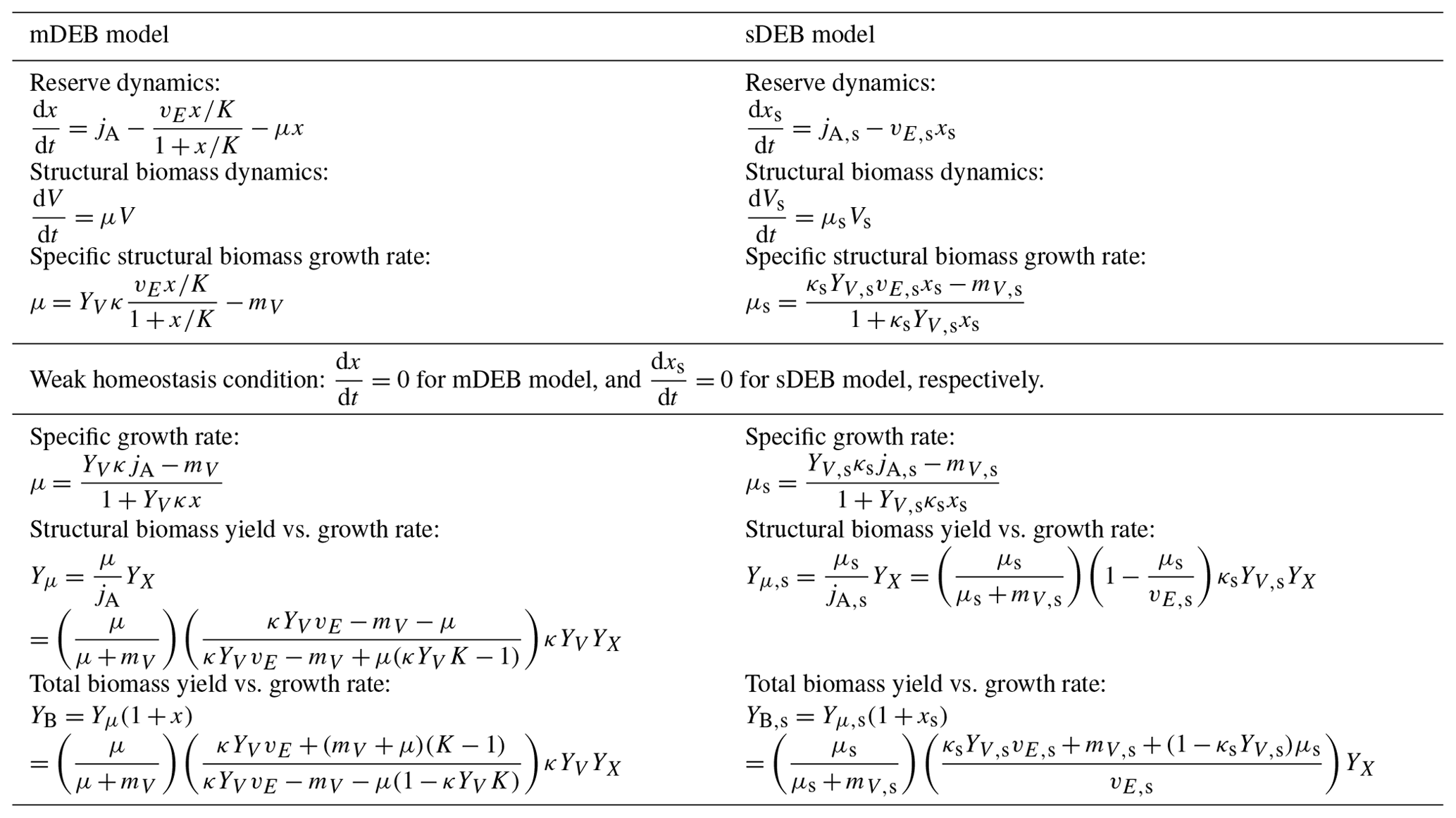
Table 1 Mathematical comparison of the mDEB and the sDEB models, with sDEB symbols annotated by subscript “s”. For both models, the κ rule for allocation to soma is applied (Kooijman, 2009). Also, it is assumed that structural biomass is proportional to the cellular population. Additionally, j_A and j_A,s have incorporated the reserve yield Y_X from substrate assimilation.

Last, we highlight that j_E,x in the mDEB model (see Eq. 6) has no explicit dependence on growth rate μ. In contrast, in the sDEB model, based on a pure mathematical argument (see Sect. 2.3.1 in Kooijman, 2009), $j_{E,x}+\mathit{\mu }x$ is formulated as a linear function of reserve density x such that j_E,x depends linearly on growth rate μ. This difference offers mDEB a significant computational advantage for modeling biological organisms growing on multiple complementary nutrients, such as carbon, nitrogen, phosphorus, sulfur, and even silicon (Madigan et al., 2009).

2.2 Growth under weak homeostasis

Under weak homeostasis, as food density is constant, specific reserve assimilation from external substrates j_A is constant, leading to $\frac{\mathrm{d}x}{\mathrm{d}t}=\mathrm{0}$. When these conditions are applied to Eq. (6), one obtains

$$\begin{array}{}\text{(8)}& j_{E,x}={\displaystyle \frac{v_{E}x}{K+x}}=j_{\mathrm{A}}-\mathit{\mu }x,\end{array}$$

which, when substituted into the dynamic energy budget Eq. (7), leads to

$$\begin{array}{}\text{(9)}& \mathit{\mu }=Y_V(j_{\mathrm{A}}-\mathit{\mu }x)-m_V\end{array}$$

such that

$$\begin{array}{}\text{(10)}& \mathit{\mu }={\displaystyle \frac{Y_V{j}_{\mathrm{A}}-m_V}{\mathrm{1}+Y_{V}x}}.\end{array}$$

Equation (10) states that under constant food density, the mDEB model predicts that growth continues with constant reserve density, just as predicted by the sDEB theory and required by the assumed weak homeostasis.

From Eqs. (8) and (9), the reserve density x can be found as

$$\begin{array}{}\text{(11)}& x={\displaystyle \frac{(\mathit{\mu }+m_V)K}{Y_V{v}_E-\mathit{\mu }-m_V}}.\end{array}$$

When Eq. (11) is entered into Eq. (9), one finds

$$\begin{array}{}\text{(12)}& \begin{array}{rl}{\displaystyle }{j}_{\mathrm{A}}& {\displaystyle }={\displaystyle \frac{\mathit{\mu }+m_V}{Y_V}}+\mathit{\mu }x\\ {\displaystyle }& {\displaystyle }={\displaystyle \frac{\mathit{\mu }+m_V}{Y_V}}{\displaystyle \frac{Y_V{v}_E-m_V-\mathit{\mu }(\mathrm{1}-K{Y}_V)}{Y_V{v}_E-m_V-\mathit{\mu }}}.\end{array}\end{array}$$

Equation (12) can be used to derive the yield of structural biomass (or population) under weak homeostasis:

$$\begin{array}{}\text{(13)}& \begin{array}{rl}{\displaystyle }{Y}_{\mathit{\mu }}& {\displaystyle }={\displaystyle \frac{\mathit{\mu }}{j_{\mathrm{A}}}}{Y}_X\\ {\displaystyle }& {\displaystyle }=\left({\displaystyle \frac{\mathit{\mu }}{\mathit{\mu }+m_V}}\right)\left({\displaystyle \frac{Y_V{v}_E-m_V-\mathit{\mu }}{Y_V{v}_E-m_V-\mathit{\mu }+Y_{V}K\mathit{\mu }}}\right)Y_V{Y}_X,\end{array}\end{array}$$

where Y_X is the reserve biomass yield for assimilating substrate from the environment.

Accordingly, the yield for total biomass is

$$\begin{array}{}\text{(14)}& \begin{array}{rl}{\displaystyle }{Y}_{\mathrm{B}}& {\displaystyle }=Y_{\mathit{\mu }}(\mathrm{1}+x)\\ {\displaystyle }& {\displaystyle }=\left({\displaystyle \frac{\mathit{\mu }}{\mathit{\mu }+m_V}}\right)\left({\displaystyle \frac{Y_V{v}_E+(m_V+\mathit{\mu })(K-\mathrm{1})}{Y_V{v}_E-m_V-\mathit{\mu }+Y_{V}K\mathit{\mu }}}\right)Y_V{Y}_X.\end{array}\end{array}$$

Since the mDEB model is compatible with the weak homeostasis assumption, like the sDEB model, it is naturally compatible with the Von Bertalanffy growth model that relates the size of an organism to its age at constant specific food supply (see Sect. 2.6.1 in Kooijman, 2009). Moreover, under the assumed weak homeostasis, since j_A is constant, the specific growth rate μ can be solved from the equation of Y_μ for the mDEB model in Table 1 (which can be verified to be a quadratic equation of μ; see its special case in Eq. 21).

2.3 mDEB model for K≫x

We next apply the condition K≫x to derive some special case analytical results of the mDEB model. (We note that the condition K≫x corresponds to the high enzyme condition that is usually satisfied inside biological cells (Tang and Riley, 2023; Phillips et al., 2012), even though it is not essential for the application of the mDEB model.) Specifically, we may define ${\stackrel{\mathrm{̃}}{v}}_E=v_E/K$ so that Eq. (6) becomes

$$\begin{array}{}\text{(15)}& {\displaystyle \frac{\mathrm{d}x}{\mathrm{d}t}}=j_{\mathrm{A}}-{\stackrel{\mathrm{̃}}{v}}_{E}x-\mathit{\mu }x,\end{array}$$

and Eq. (7) becomes

$$\begin{array}{}\text{(16)}& \mathit{\mu }=Y_V{\stackrel{\mathrm{̃}}{v}}_{E}x-m_V.\end{array}$$

For growth under weak homeostasis (i.e., $\frac{\mathrm{d}x}{\mathrm{d}t}=\mathrm{0}$), one then has

$$\begin{array}{}\text{(17)}& x={\displaystyle \frac{\mathit{\mu }+m_V}{Y_V{\stackrel{\mathrm{̃}}{v}}_E}},\end{array}$$

and

$$\begin{array}{}\text{(18)}& j_{\mathrm{A}}=({\stackrel{\mathrm{̃}}{v}}_E+\mathit{\mu })x=\left({\displaystyle \frac{{\stackrel{\mathrm{̃}}{v}}_E+\mathit{\mu }}{{\stackrel{\mathrm{̃}}{v}}_E}}\right)\left({\displaystyle \frac{\mathit{\mu }+m_V}{Y_V}}\right),\end{array}$$

and, accordingly, the structural biomass yield is

$$\begin{array}{}\text{(19)}& Y_{\mathit{\mu }}={\displaystyle \frac{\mathit{\mu }}{j_{\mathrm{A}}}}{Y}_X=\left({\displaystyle \frac{\mathit{\mu }}{\mathit{\mu }+m_V}}\right)\left({\displaystyle \frac{{\stackrel{\mathrm{̃}}{v}}_E}{{\stackrel{\mathrm{̃}}{v}}_E+\mathit{\mu }}}\right)Y_V{Y}_X,\end{array}$$

and the total biomass yield is

$$\begin{array}{}\text{(20)}& \begin{array}{rl}{\displaystyle }{Y}_{\mathrm{B}}& {\displaystyle }=Y_{\mathit{\mu }}(\mathrm{1}+x)\\ {\displaystyle }& {\displaystyle }=\left({\displaystyle \frac{\mathit{\mu }}{\mathit{\mu }+m_V}}\right)\left({\displaystyle \frac{Y_V{\stackrel{\mathrm{̃}}{v}}_E+\mathit{\mu }+m_V}{{\stackrel{\mathrm{̃}}{v}}_E+\mathit{\mu }}}\right)Y_X.\end{array}\end{array}$$

Additionally, from Eq. (18), one can obtain

$$\begin{array}{}\text{(21)}& \mathit{\mu }={\displaystyle \frac{m_V+{\stackrel{\mathrm{̃}}{v}}_E}{\mathrm{2}}}\left(-\mathrm{1}+\sqrt{\mathrm{1}+{\displaystyle \frac{\mathrm{4}{\stackrel{\mathrm{̃}}{v}}_E(j_{\mathrm{A}}{Y}_V-m_V)}{(m_V+{\stackrel{\mathrm{̃}}{v}}_E{)}^{\mathrm{2}}}}}\right).\end{array}$$

3 Comparisons with the sDEB model

3.1 Biological growth on single reserve

The mDEB model is compared to the sDEB model for growth from a single reserve pool in Table 1. That comparison shows that the two models have the same equation for specific growth rate (μ vs. μ_s) only under weak homeostasis (when the reserve density reaches steady state and thus the whole organism is of fixed elemental stoichiometry, i.e., $\frac{\mathrm{d}{x}_{\mathrm{s}}}{\mathrm{d}t}=\mathrm{0}$ for the sDEB model and $\frac{\mathrm{d}x}{\mathrm{d}t}=\mathrm{0}$ for the mDEB model), and, mathematically, the two models are structurally very similar.

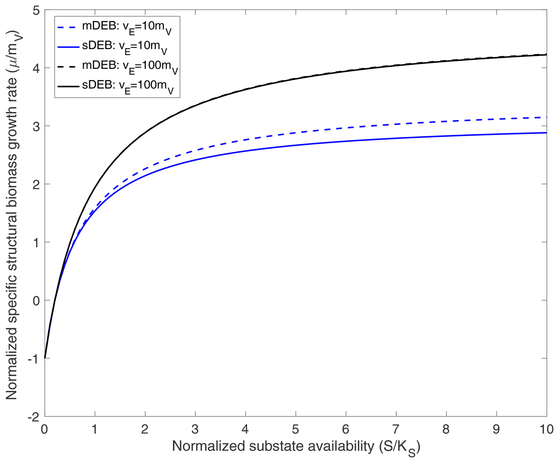
Figure 1 Comparison of predicted specific structural biomass growth rate as a function of normalized substrate availability under weak homeostasis conditions. For cases with v_E=10m_V, specific reserve turnover rate is 10 times the specific structural biomass maintenance rate. For cases with v_E=100m_V, specific reserve turnover rate is 100 times the specific structural biomass maintenance rate. The mDEB model is based on Eq. (21), while the sDEB model is based on ${\mathit{\mu }}_{\mathrm{s}}=\frac{Y_{V,\mathrm{s}}{j}_{\mathrm{A},\mathrm{s}}-m_{V,\mathrm{s}}}{\mathrm{1}+Y_{V,\mathrm{s}}{j}_{\mathrm{A},\mathrm{s}}/v_{E,\mathrm{s}}}$. In producing the above results, for both j_A and j_A,s, the Michaelis–Menten kinetics $f\left(S\right)=j_{\mathrm{A},max}S/(S+K_S)$ are used for substrate uptake.

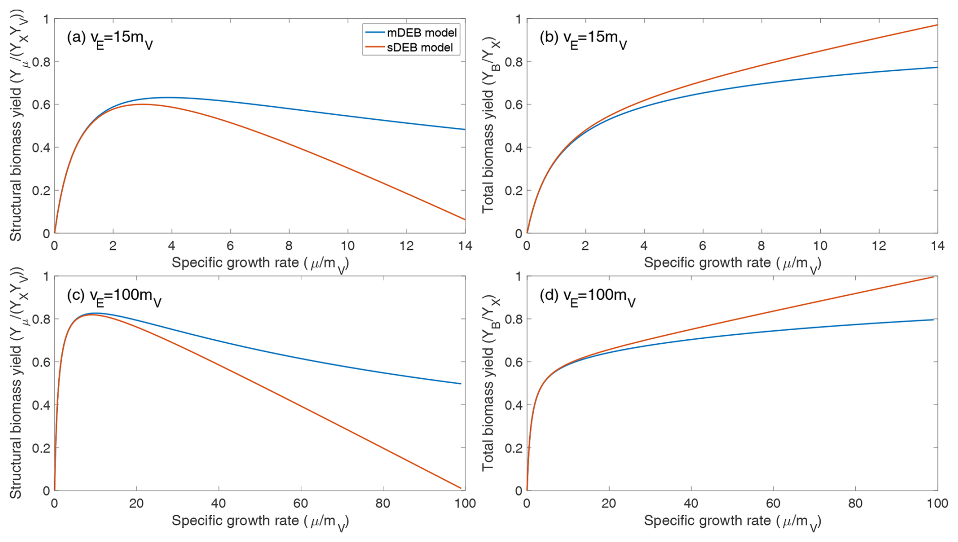
Figure 2 Comparison of predicted biomass yield as a function of normalized specific growth rate under weak homeostasis conditions. (a, c) Predicted relationship between structural biomass yield and specific growth rate. (b, d) Predicted relationship between total biomass yield and specific growth rate. Y_X is the reserve biomass yield for substrate assimilation from the environment. For both models, it is assumed that the structural biomass yield from reserve biomass is 0.6. (a, b) The maximum specific reserve turnover rate is 15 times the specific structural biomass maintenance rate. (c , d) The maximum specific reserve turnover rate is 100 times the specific structural biomass maintenance rate.

Under the weak homeostasis condition, because reserve density is time-invariant and depends algebraically on reserve assimilate rate (j_A), the mDEB and sDEB models predict the specific structural biomass growth rate as a function of substrate concentration in a pattern very similar to that predicted using Monod kinetics (Fig. 1; Monod, 1949). When the specific reserve turnover rate is much greater than the specific maintenance rate, the mDEB model for K≫x and the sDEB model predict almost identical growth rates as a function of substrate availability (lines with v_E=100m_V in Fig. 1).

Moreover, the two models predict very similar relationships between specific growth rate and both structural biomass yield and total biomass yield under weak homeostasis (Fig. 2). Specifically, under weak homeostasis conditions, both the mDEB and sDEB models predict that the structural biomass yield first increases, then plateaus, and then decreases with specific growth rate (Fig. 2a and c), with the sDEB model predicting a faster decrease at higher growth rate. The total biomass yield increases almost hyperbolically with specific growth rate (Fig. 2b and d), with the sDEB model predicting a faster increase at higher growth rate. We note that the relationship between total biomass yield and specific growth rate is consistent with that predicted by the empirical compromise model (Beeftink et al., 1990; Wang and Post, 2012). The qualitative difference between structural biomass yield and total biomass yield suggests that more analysis is needed of how they may affect simulated biogeochemistry.

3.2 Biological growth on two reserves

When an organism is growing on two complementary reserves (from assimilation two complementary substrates, e.g., carbon and nitrogen), the growth rate may be computed using the synthesizing unit kinetics (Kooijman, 2009) such that

$$\begin{array}{}\text{(22)}& \mathit{\mu }={\left(j_{G,x_{\mathrm{1}}}^{-\mathrm{1}}+j_{G,x_{\mathrm{2}}}^{-\mathrm{1}}-(j_{G,x_{\mathrm{1}}}+j_{G,x_{\mathrm{2}}}{)}^{-\mathrm{1}}\right)}^{-\mathrm{1}}.\end{array}$$

For simplicity, in Eq. (22) we assume that the specific growth rate μ is positive. Negative growth when reserve fluxes fall short of maintenance requirements can be considered separately (Tolla et al., 2007; Kooijman, 2009).

By designating the maintenance flux required for reserve x₁ and x₂ as $j_{M,x_{\mathrm{1}}}$ and $j_{M,x_{\mathrm{2}}}$, one has

$$\begin{array}{}\text{(23)}& j_{G,x_i}=y_{G,x_i}(j_{E,x_i}-j_{M,x_i}),i=\mathrm{1},\mathrm{2},\end{array}$$

where $y_{G,x_i}$ is the stoichiometric yield of transforming reserve x_i into structural biomass.

When Eqs. (22) and (23) are applied with the mDEB model, according to Eq. (4), $j_{E,x_i}$ is independent of specific growth rate μ so that μ is an explicit function of fluxes $j_{E,x_i}$ and $j_{M,x_i}$. (Therefore, the mDEB model never requires iterations for solving μ, whether $j_{E,x_i}$ is a linear or nonlinear function of reserve density x_i.) In contrast, when the sDEB model is applied, $j_{E,x_i}$ is a function of μ:

$$\begin{array}{}\text{(24)}& j_{E,x_i}=(v_E-\mathit{\mu })x_i.\end{array}$$

Therefore, for the sDEB model, Eqs. (22)–(24) indicate that μ is an implicit function, whose solution requires numerical iteration for each calculation of growth rate μ (also see equation of μ_g for the sDEB model in Table 2). Furthermore, as the sDEB model strives to include more organisms and more complementary reserves, e.g., biological growth that is concurrently regulated by pools of carbon, nitrogen, and phosphorus (as many existing biogeochemical models attempt; e.g., Goll et al., 2012; Yu et al., 2020; Zhu et al., 2019; Mekonnen et al. 2019), the necessity of iteration to explicitly represent many numbers of biological organisms will make the growth rate in the sDEB model increasingly more cumbersome to solve. In contrast, the absence of numerical iteration in the mDEB model will significantly simplify this aspect of the modeling processes.

Table 2 A mDEB model of diatom T. weissflogii growing on CO₂ and inorganic nitrogen. For comparison, also given are sDEB model equations for growth and reserve dynamics.

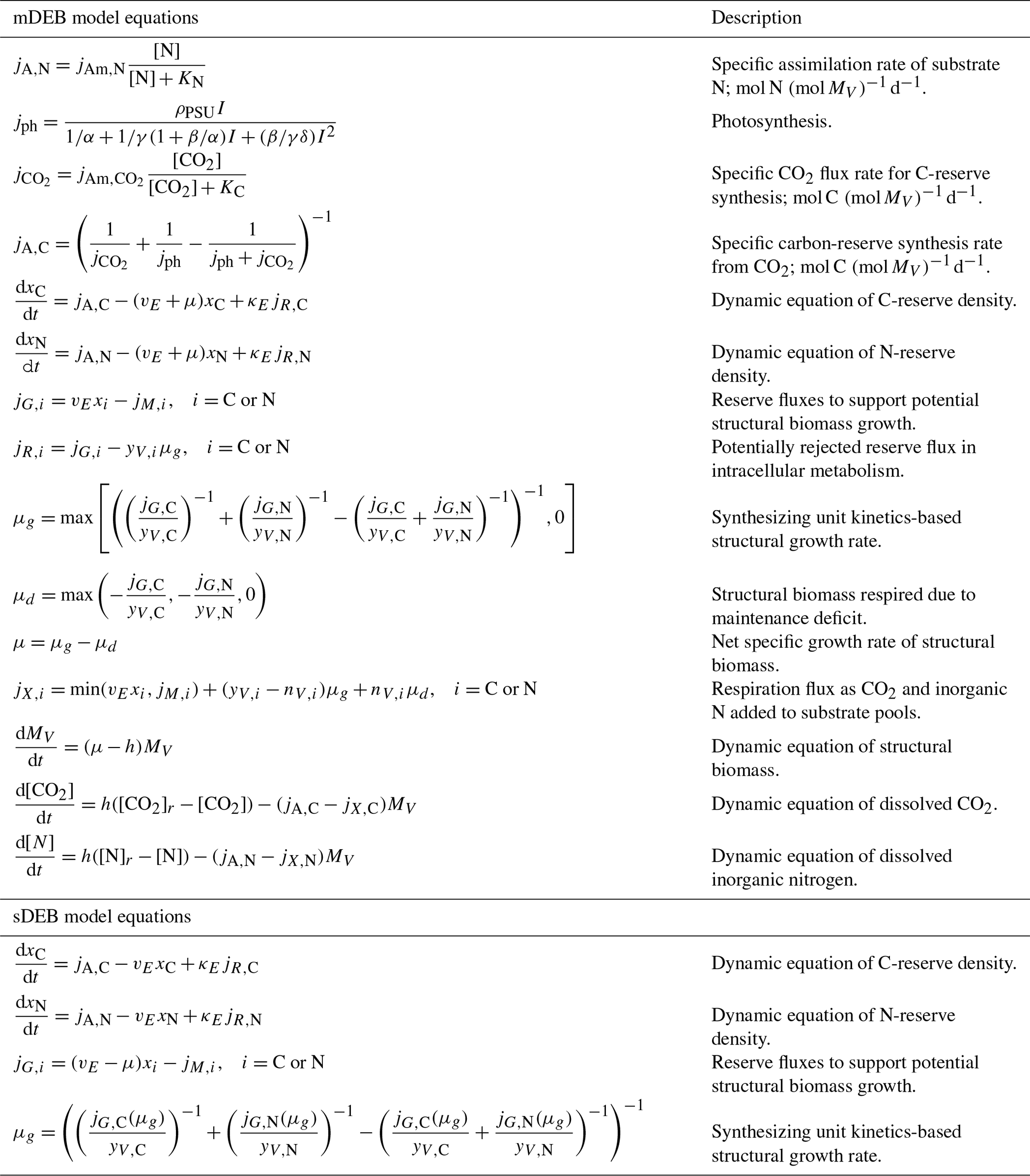
Table 3 Parameters of the mDEB model. The values of v_E were found by manual tuning, with the sDEB model value in parentheses. All other parameters are the same as in Lorena et al. (2010).

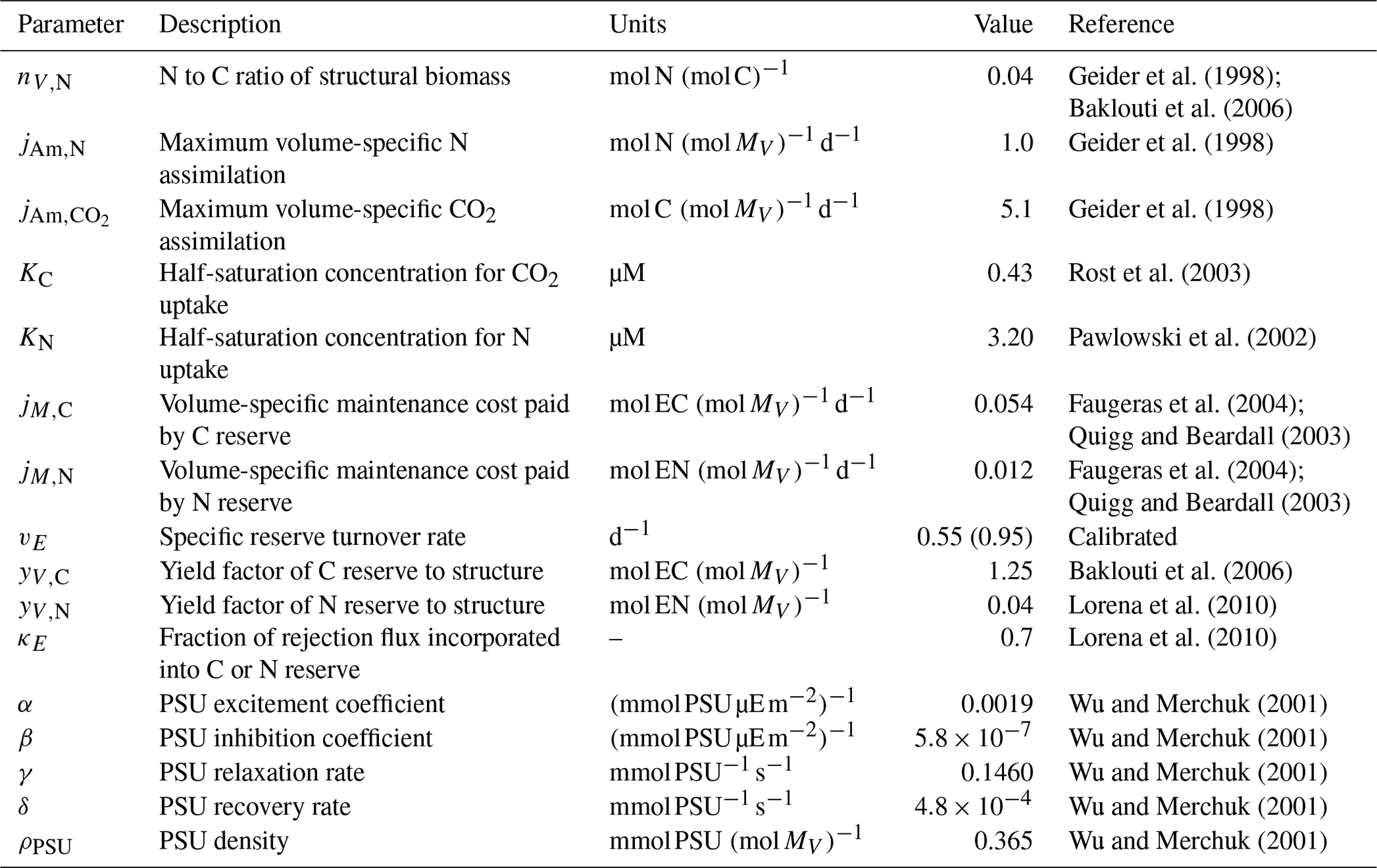
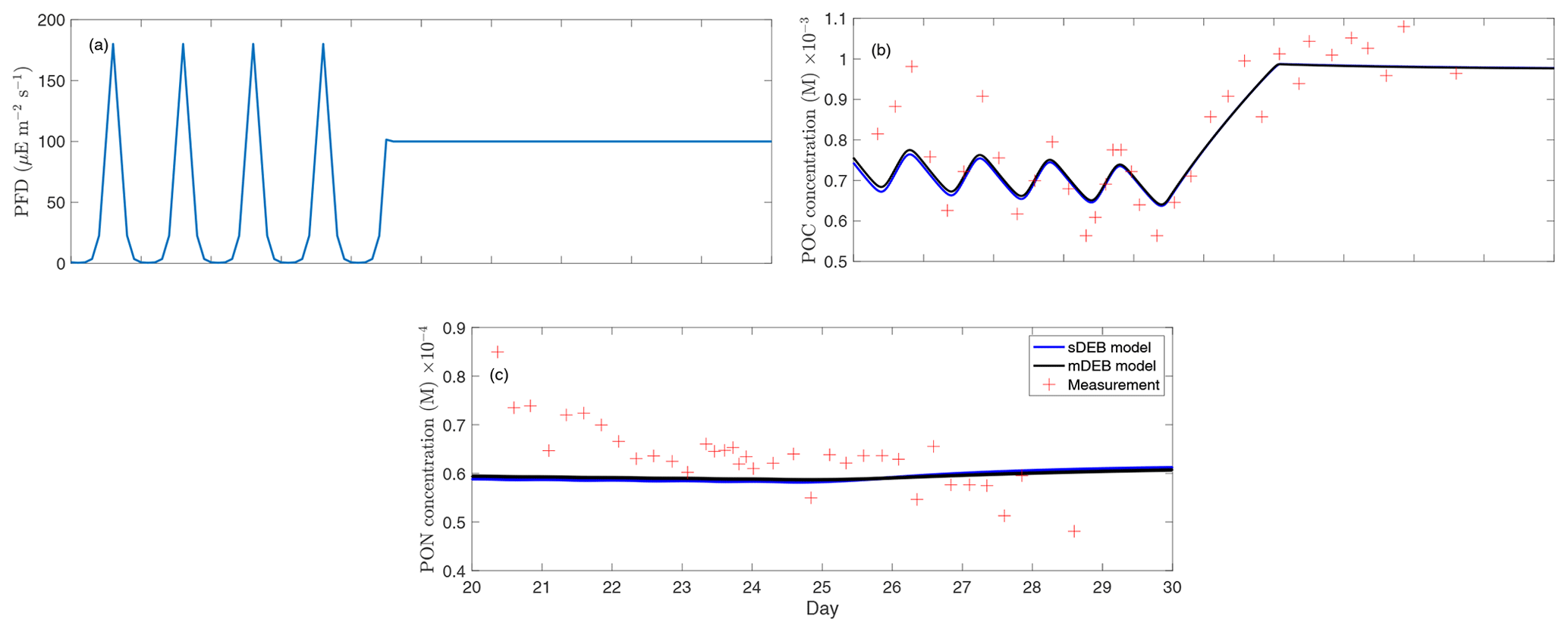
Figure 3 Model–data comparison for the chemostat experiment of T. weissflogii from Pawlowski (2004). (a) Photon flux density (PFD) over the measurement period, (b) particulate organic carbon (reserve plus structural biomass carbon; POC) of the T. weissflogii population, and (c) particulate organic nitrogen (reserve plus structural biomass nitrogen; PON) of the T. weissflogii population. All panels only show results over the time period when measurements were available.

To demonstrate the applicability of mDEB model on biological growth over multiple complementary substrates, we constructed a mDEB model for the chemostat experiment of the diatom Thalassiosira weissflogii (T. weissflogii) from Pawlowski (2004). Like the sDEB model by Lorena et al. (2010), the mDEB model (Table 2) makes the following assumptions:

1. When the mobilized reserve fluxes fall short of the demand from maintenance, structural biomass is reduced proportional to the deficit (as the maximum deficit of two reserves), and this reduced structural biomass is mineralized immediately into substrates.

2. The fraction of rejected reserve that is not returned to reserve is not mineralized to become substrates.

The mDEB model adopts almost identical parameter values from the sDEB model (compare our Table 3 with their Table 2), except that the mDEB model sets the specific reserve turnover rate (v_E) to 0.55 d⁻¹, calculated by manual tuning, while the sDEB model in Lorena et al. (2010) used a value of 2.60 d⁻¹. For comparison, we also coded a sDEB model that differs from the mDEB model only in the computation of growth rate, which is achieved through the bisection algorithm (Burden and Faires, 1985). Because we adopted a formulation of negative growth rate μ_d different from Lorena et al. (2010) (See their Eq. 2.11, where they assumed that negative growth rates from carbon reserve deficit and nitrogen reserve deficit are additive. However, we used the maximum of the two instead), the sDEB model here used 0.95 d⁻¹ for the specific reserve turnover rate.

By using parameters mostly from the literature, we find that the mDEB model predictions captured the measured time series of particulate organic carbon and nitrogen reasonably (Fig. 3). While better model–data agreement may be obtained by optimizing more parameters, the results here suggest that the mDEB model is at least as capable as the sDEB model. Interestingly, the sDEB model here produced almost identical model–data agreement. Moreover, for the 30 d simulation period, the mDEB model took about 55 % of the time of the sDEB model. On an Apple M3 Max machine with 64 GB memory, using MatlabR2020b, the typical execution times are 0.037 and 0.068 s for the mDEB model and sDEB model, respectively. (We provide the source code for readers to play with the models.) This significant improvement in computational efficiency and good model–data agreement thus suggests the mDEB model is a good replacement for the sDEB model.

4 Conclusions

Starting with the mass conservation equation from the nonequilibrium thermodynamics, the law of mass action, and the basic assumptions of the dynamic energy budget theory, we derived a modified formulation of the dynamic energy budget (mDEB) model. The mDEB model is mathematically very similar to the standard dynamic energy budget (sDEB) model and is able to recover many of the features of the sDEB model. However, because it does not require numerical iterations for the computation of growth rate, particularly for biological growth that involves multiple complementary substrates, the mDEB model is computationally much more efficient. In the example application to a chemostat experiment of T. weissflogii, the mDEB and sDEB models are found equally accurate, while the former only required almost half the computing time of the latter. Moreover, since the mDEB model is compatible with non-linear kinetics for reserve turnover, it can be extended to models that consider ribosome allocation explicitly for microbes (Tadmor and Tlusty, 2008).

With its strong theoretical foundation and easier numerical implementation, we expect that the mDEB model will consistently formulate biological growth of microbes, plants, and animals (which are all in the application domain of the DEB theory; Kooijman, 2009; Yang et al., 2020; Russo et al., 2022; Matyja and Lech, 2024). Coupled with the reactive transport-based modeling of substrate transport and aqueous chemistry, we believe the consistent application of the mDEB model will significantly alleviate the structural uncertainty of ecosystem biogeochemical models, as envisioned in Tang et al. (2024).

Appendix A: Nomenclature

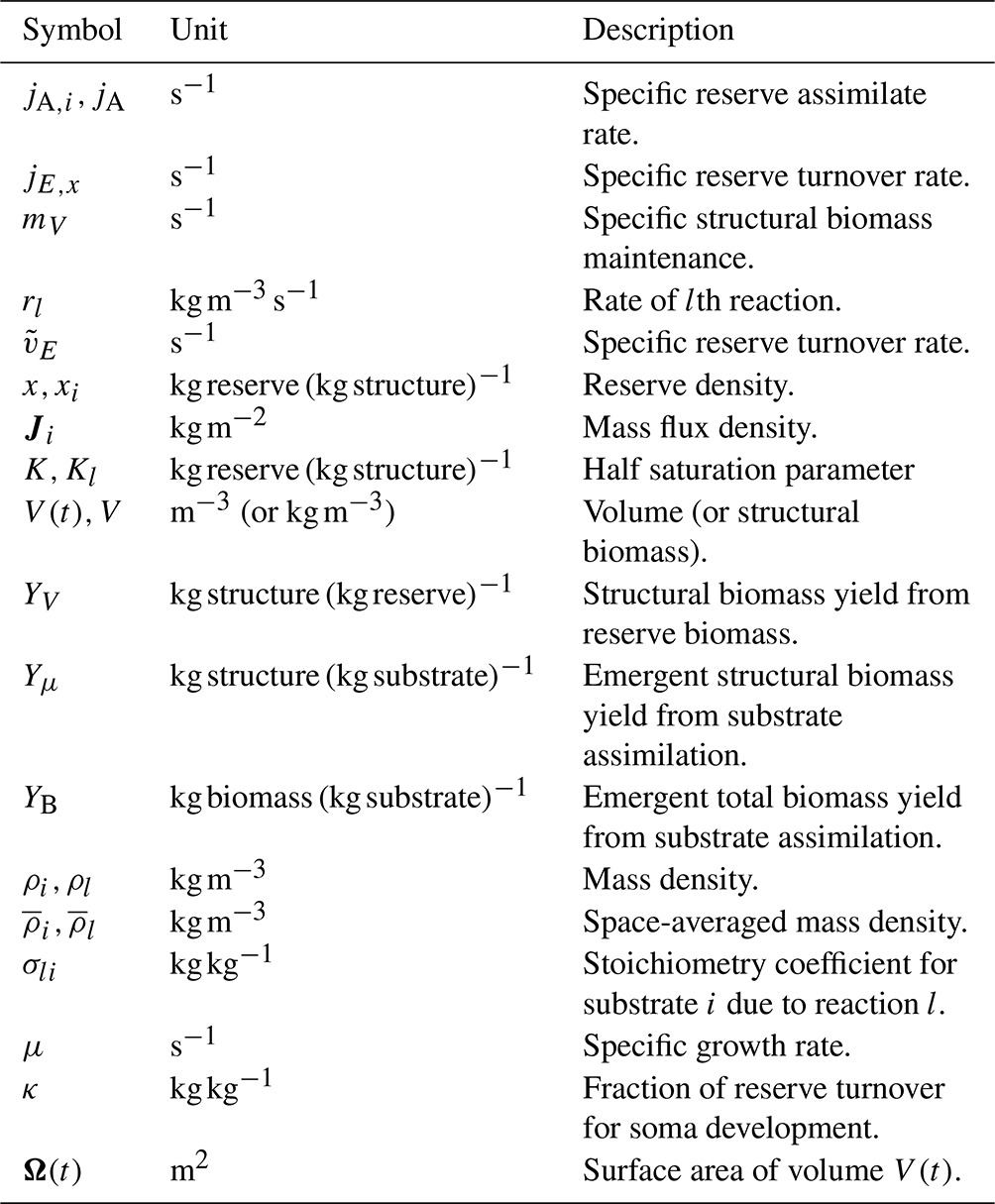
Table A1 This table only includes symbols not defined in Tables 2 and 3.