the Creative Commons Attribution 4.0 License.
the Creative Commons Attribution 4.0 License.
 | 19 Jun 2025
Assessing the lifetime of anthropogenic CO2 and its sensitivity to different carbon cycle processes
Christine Kaufhold
Matteo Willeit
Andrey Ganopolski
Although it is well-established that anthropogenic CO2 emitted into the atmosphere will persist for a long time, the duration of the anthropogenic climate perturbation will depend on how rapidly the excess CO2 is removed from the climate system by different biogeochemical processes. The uncertainty around the long-term climate evolution is therefore linked to not only the future of anthropogenic CO2 emissions but also our insufficient understanding of the long-term carbon cycle. Here, we use the fast Earth system model CLIMBER-X, which features a comprehensive carbon cycle, to examine the lifetime of anthropogenic CO2 and its effects on the long-term evolution of atmospheric CO2 concentration. This is done through an ensemble of 100 000-year-long simulations, each driven by idealized CO2 emission pulses. Our findings indicate that depending on the magnitude of the emission, 75 % of anthropogenic CO2 is removed within 197–1820 years of the peak CO2 concentration (with larger cumulative emissions taking longer to remove). Approximately 4.3 % of anthropogenic CO2 will remain beyond 100 kyr. We find that the uptake of carbon by land, which has only been considered to a small extent in previous studies, has a significant long-term effect, storing approximately 4 %–13 % of anthropogenic carbon by the end of the simulation. Higher-emission scenarios fall on the lower end of this range, as increased soil respiration leads to greater carbon loss. For the first time, we have quantified the effect of dynamically changing methane concentrations on the long-term carbon cycle, showing that its effects are likely negligible over long timescales. The timescale of carbon removal via silicate weathering is also reassessed here, providing an estimate (80–105 kyr) that is significantly shorter than some previous studies due to higher climate sensitivity, stronger weathering feedbacks, and the use of a spatially explicit weathering scheme, leading to faster removal of anthropogenic CO2 in the long term. Furthermore, this timescale is shown to have a non-monotonic relationship with cumulative emissions. Our study highlights the importance of adding model complexity to the global carbon cycle in Earth system models to accurately represent the long-term future evolution of atmospheric CO2.
- Article
(15968 KB) - Full-text XML
- BibTeX
- EndNote


A large amount of research has been dedicated to studying the impact of anthropogenic CO2 emissions on the climate, what oceanographer Roger Revelle stated was “man's great geophysical experiment” (Revelle, 1956; Revelle et al., 1965). The scope of such research is usually limited to centennial timescales due to their relevance for governance and policy. However, there is a growing societal need for and an increasing number of scientific inquiries into the long-term (> 103 years) future. This concerns the site selection for nuclear waste disposal and post-closure safety assessments of deep geological repositories in particular, as a number of environmental factors, such as subterranean stress, permafrost, erosion, and subrosion, can potentially compromise long-term safety (Näslund et al., 2013; Lord et al., 2015a; Lindborg et al., 2018; Turner et al., 2023; Kurgyis et al., 2024).
Previous studies on long-term future climate evolution have primarily focused on one of two tightly related research areas. Some, for example, have investigated the length of the current interglacial period under natural conditions: Berger and Loutre (2002) showed that we were already positioned to experience an unusually prolonged interglacial period as we currently approach a minima in the 100 and 400 kyr eccentricity cycle. A second area of interest is the lifetime of anthropogenic CO2 in the atmosphere1: Archer et al. (1997) and Archer et al. (1998) improved previous estimates by including CaCO3 dissolution kinetics and showed that the return of the atmospheric CO2 concentration to pre-industrial conditions would take tens of thousands of years. These two overarching areas of focus converged in Archer (2005) and Archer and Ganopolski (2005), where they showed that (1) not only is anthropogenic CO2 expected to survive in our atmosphere for several hundreds of thousands of years but (2) it could also significantly delay the next glacial period. This was later confirmed by other studies (Ganopolski et al., 2016; Talento and Ganopolski, 2021).
In the past, general circulation models (GCMs) and intermediate complexity models (EMICs) have been used to study the 1000–10 000 year carbon cycle response to anthropogenic CO2 emissions (see Archer et al., 2009a; Joos et al., 2013). Modelling studies become more scarce when going even further forward in time due to the rising computational cost, and as such, experiments are based on either EMICs (Ridgwell and Hargreaves, 2007; Charbit et al., 2008; Eby et al., 2009; Shaffer, 2010; Goodwin and Ridgwell, 2010; Meissner et al., 2012; Ganopolski et al., 2016; Brault et al., 2017; Jeltsch-Thömmes and Joos, 2020; Duque-Villegas et al., 2022) or models of lower complexity (Sundquist, 1991; Walker and Kasting, 1992; Lenton and Britton, 2006; Tyrrell et al., 2007a; Uchikawa and Zeebe, 2008; Cawley, 2011; Herrero et al., 2013; Köhler, 2020; Talento and Ganopolski, 2021; Couplet et al., 2025). The results of these studies largely agree in some aspects. For example, it has been established that the magnitude of cumulative emissions rather than the emission pathway will predominantly control the long-term response (Eby et al., 2009; Matthews et al., 2009; Zickfeld et al., 2012; Herrington and Zickfeld, 2014). Contemporary predictions for deep-future CO2 concentrations exhibit considerable diversity, however. For illustration, Fig. 1 provides a graphical overview of the current estimates of atmospheric CO2 concentration 10 000 years after the present for different cumulative CO2 emissions.
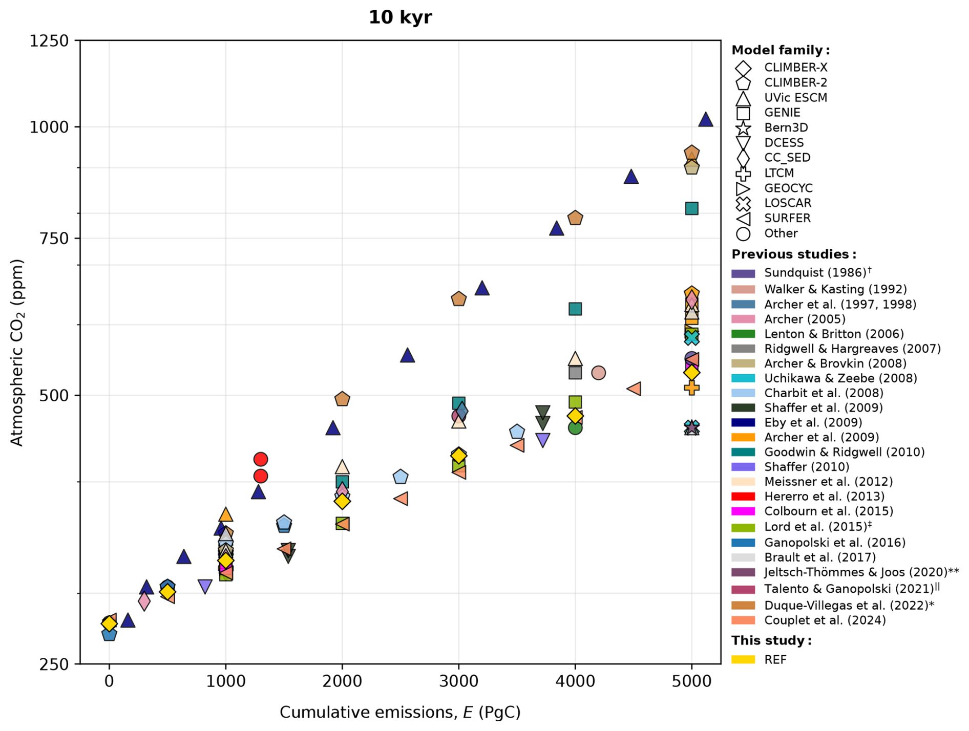
Figure 1Estimates on the impact of different cumulative emissions on atmospheric CO2 concentration 10 kyr after the start of the simulation. The data from previous studies shown here were acquired through visual inspection of graphs, meaning that the figure is semi-qualitative and mostly serves an illustrative purpose (small errors may be present). Experiments shorter than 10 000 years or those that considered emissions of 6000 Pg C or larger (i.e., unconventional fossil fuel resources) were omitted. Different experiments were chosen from these publications to highlight the fact that the large diversity is primarily due to how long-term carbon cycle processes are resolved. The reference experiment in this study (yellow) has been plotted for comparison. Further information can be found in the respective publications. † Data for Sundquist (1991) taken from Tyrrell et al. (2007a). ‡ Data generated from the emulator based on cGENIE results. Data calculated from the fraction of emissions remaining. ‖ Best solution from the model ensemble. * Data calculated from the formula provided in the appendix of Duque-Villegas et al. (2022).
Quantifying the atmospheric lifetime of anthropogenic CO2 is challenging because it is controlled by a number of biochemical and geological mechanisms operating on different timescales up to hundreds of thousands of years (Archer et al., 2009a). Modelling studies suggest that the terrestrial biosphere will initially take up anthropogenic CO2 (owing to enhanced vegetation productivity from CO2 fertilization), although increased cellular respiration, soil carbon decomposition, land use change, and wildfires could eventually turn the land into a carbon source in a warming world. Extensive fossil fuel emissions can therefore overpower the capacity of conventional land carbon reservoirs to absorb anthropogenic CO2, and only the ocean remains as the CO2 sink on long timescales through processes such as air–sea CO2 exchange, ocean invasion, seafloor CaCO3 reactions, and carbonate accumulation. The substantial influence that marine biogeochemistry has on the long-term carbon cycle has also been recognized by many studies, in particular regarding the reaction between dissolved anthropogenic CO2 and calcium carbonate in deep-ocean sediments (Archer et al., 1997; Middelburg et al., 2020). On even longer timescales, carbon exchange with geological reservoirs becomes important through processes such as sediment burial, chemical weathering of rocks on land, and volcanic degassing. As a consequence of all of these processes, carbon cycle models predict a highly nonlinear removal of anthropogenic CO2 over time. The decline in anthropogenic CO2 is usually presented as a superposition of exponential decays (Maier-Reimer and Hasselmann, 1987; Archer et al., 1997; Archer and Brovkin, 2008; Colbourn et al., 2015; Lord et al., 2015b), with each function representing a different process in the carbon cycle that takes up carbon. This generally produces a long tail of anthropogenic CO2 concentration, which has been shown to persist for hundreds of thousands of years.
Due to the complexity and variety of poorly understood processes, the long-term future climate evolution remains highly uncertain even when not considering the unpredictability of future anthropogenic emissions (which can be reconciled to some extent using an ensemble of emission scenarios). Given this complexity, it becomes essential to make assumptions based on the timescales involved, the specific research question being addressed, and the resolution of the model employed. Previous studies have often made significant simplifications to (e.g., Lenton and Britton, 2006) or completely neglected (e.g., Archer et al., 1997; Lord et al., 2015b; Köhler, 2020) certain aspects related to land carbon. Weathering processes have also been frequently simplified (e.g., Charbit et al., 2008; Uchikawa and Zeebe, 2008) or their feedbacks not considered (e.g., Montenegro et al., 2007; Ridgwell and Hargreaves, 2007; Eby et al., 2009). As computational expense is the biggest factor inhibiting high-resolution modelling on longer timescales, these studies also did not consider the interaction between CO2 and ice sheets, methane deposits, and the effect of future glacial cycles (Archer, 2005).
Here, we provide a set of idealized long-term transient climate change scenarios for the next 100 000 years using the fast Earth system model CLIMBER-X with a comprehensive carbon cycle model. These experiments seek to quantify the degree of uncertainty in the anthropogenic factor by employing a wide range of idealized emission scenarios to evaluate the spread in possible climate responses. Considering the ongoing and substantial disagreement regarding future CO2 evolution among different models, we provide an analysis of the sensitivity of the model response to climate sensitivity and different carbon cycle processes. This is a first step towards a fully coupled simulation of the next 100 kyr with CLIMBER-X, which includes interactive ice sheets. The paper is structured as follows: we first describe our experimental setup, model, and considerations (Sect. 2). The results are then contextualized in relation to other studies by analyzing the model response, atmospheric lifetime, and subsequent removal timescales of different carbon cycle processes (Sect. 3). This is followed by a corresponding sensitivity study (Sect. 4). We conclude with a brief discussion, summary of our findings, and an outlook on further investigations (Sect. 5).
2.1 Model description
We use CLIMBER-X v1.1 (Willeit et al., 2022, 2023), a fast Earth system model designed to simulate the climate evolution on timescales ranging from decades to > 100 000 years. CLIMBER-X includes the statistical–dynamical semi-empirical atmosphere model SESAM (Willeit et al., 2022), the 3D frictional–geostrophic ocean model GOLDSTEIN (Edwards et al., 1998; Edwards and Marsh, 2005), the dynamic–thermodynamic sea ice model SISIM (Willeit et al., 2022), the land surface and dynamic vegetation model PALADYN (Willeit and Ganopolski, 2016), and the ocean biogeochemistry and marine sediment model HAMOCC (Heinze and Maier-Reimer, 1999; Ilyina et al., 2013; Mauritsen et al., 2019). CLIMBER-X operates at a horizontal resolution of 5°×5°. It is computationally efficient and can simulate up to 10 000 years per day, allowing it to perform a large ensemble of long-term simulations. This is also possible because short-term processes (e.g., weather, diurnal cycle) are not resolved. CLIMBER-X can generally represent historical changes in climate (Willeit et al., 2022) and the carbon cycle well (Willeit et al., 2023) and is suited to provide credible simulations for very long timescales into the deep future. Some studies using CLIMBER-X to transiently simulate the next several thousand years with a focus on the stability of the Greenland ice sheet have already been performed (e.g., Höning et al., 2023, 2024).
2.2 Open carbon cycle
The CLIMBER-X carbon cycle model has already been described in detail (Willeit et al., 2023) and has been shown to effectively represent the cycling of carbon through the atmosphere, vegetation, soils, permafrost, seawater, and marine sediments. For our experiments, we run the simulations using the open carbon cycle setup (Willeit et al., 2023), with interactive marine sediments, weathering on land, and the resulting geological sources and sinks of carbon. Carbon is not conserved in this setup; it is removed from the system through sediment burial and introduced into the system via weathering, volcanic outgassing, and anthropogenic emissions. In the open carbon cycle setup, a simplification is made to ensure that the budgets for silicate and phosphorus within the ocean–sediment system are balanced. This was done by disabling riverine fluxes of phosphorus and silicate and by assuming that organic carbon (which includes P) and opal (which includes Si) that are buried in the sediments (and, therefore, removed from the system) are instead returned to the surface ocean in remineralized form. The conservation of these inventories in the ocean–sediment system removes challenges related to nutrient conservation that would otherwise complicate the analysis and the interpretation of model results. The globally uniform atmospheric CO2 concentration in CLIMBER-X is computed interactively using source and sink terms in the following prognostic equation for the total carbon content stored as atmospheric CO2 (Catm in Pg C):
where Flnd is the global net land-to-atmosphere carbon flux (Pg C yr−1), Focn is the net sea–air carbon flux (Pg C yr−1), Fanth are anthropogenic carbon emissions (Pg C yr−1), Fvolc is the volcanic outgassing flux (Pg C yr−1), and Fweath is the CO2 consumption by carbonate and silicate weathering (Pg C yr−1) (Willeit et al., 2023). PALADYN includes a rock weathering scheme influenced by runoff and temperature (Hartmann, 2009a; Börker et al., 2020), accounting for 14 different lithologies, as described in Hartmann and Moosdorf (2012). The weathering module computes dissolved inorganic carbon (DIC) and alkalinity fluxes to the ocean based on the release of bicarbonate ions () into rivers. Spatially explicit carbonate and silicate weathering fluxes take the form
Weathering fluxes are largely described by the Arrhenius equation, with the exception of carbonate weathering for carbonate sedimentary rocks and loess, which is instead described by the runoff-dependent weathering equations from Amiotte Suchet and Probst (1995) and Börker et al. (2020), respectively. In Eqs. (2) and (3), ℓ represents the different lithologies, T is the annual mean near-surface air temperature (K), T0 is 284.2 K, Roff is the annual runoff (), b(ℓ) is the molality/weathering rate (mol C kg−1 water), Ea,carb is the activation energy of carbonates (14 kJ mol−1), Ea,sil(ℓ) is the activation energy of silicates (kJ mol−1), R is the molar gas constant (8.3145 ), α(ℓ) is the fraction to weather as carbonate rocks, and β(ℓ) is the fraction of a given lithology in a grid cell (Fig. E1). The values for α, b, and Ea are all based on the calibrated runoff- and temperature-dependent models from Hartmann (2009a) and Hartmann et al. (2014) and are displayed in Table E1.
Although the Earth experiences a number of external forces, this study generally excludes factors like impact events, changes in tectonic configuration, and solar luminosity, as they are either unpredictable or operate on such long timescales that they are not relevant for our investigation. Similarly, we do not resolve the deep-carbon cycle (i.e., carbon subduction and recycling in the Earth's mantle), as its effects only become important on timescales longer than our experiment duration (i.e., 106–107 years) and involve processes that cannot be resolved with Earth system models. As such, we assume that the pre-industrial carbon cycle was in equilibrium, which implies that the constant volcanic outgassing is prescribed and is set to half the global silicate weathering flux at the pre-industrial time (0.0738 Pg C yr−1 or 6.15 Tmol C yr−1). This condition ensures that the atmospheric CO2 is in equilibrium under pre-industrial conditions (Munhoven and François, 1994; Willeit et al., 2023), which has been a common assumption in previous investigations that looked at the long-term forced response of the climate (e.g., Colbourn et al., 2015; Lord et al., 2015b).
2.3 Experimental setup
Model simulations are started from a pre-industrial equilibrium state that has been obtained from a 100 000 year equilibrium spin-up of the carbon cycle model, as described in Willeit et al. (2023). The pre-industrial CO2 concentration is taken to be 280 ppm, whereas the pre-industrial orbital parameters of eccentricity e is 0.0167, obliquity ϵ is 23.46°, and the perihelion ω is 100.33°. This corresponds to a maximum summer insolation at 65° N of 480.4 W m−2. In the reference (REF) experiment, we set a constant methane concentration of 600 ppb, which is representative of Holocene conditions (Sapart et al., 2012; Mitchell et al., 2013; Beck et al., 2018). Although CLIMBER-X is capable of simulating ice sheets (e.g., Höning et al., 2023; Talento et al., 2024; Willeit et al., 2024), we conduct our simulations with prescribed present-day Greenland and Antarctica to ensure comparability with earlier studies. Interactive ice sheets will be enabled in a follow-up study. To simplify interpretation and ensure consistency with previous studies, orbital forcing was fixed at present-day values, with the combined effects of anthropogenic and orbital forcing to be explored in a future study. All simulations were run for 100 000 years, with constant orbital parameters and without any climate acceleration technique.
Table 1Overview of the experimental configuration for the simulations performed in this study. For each experimental configuration, all emission forcings (0–5000 Pg C) were applied to produce an ensemble. Emissions pathways are shown in Fig. E2.
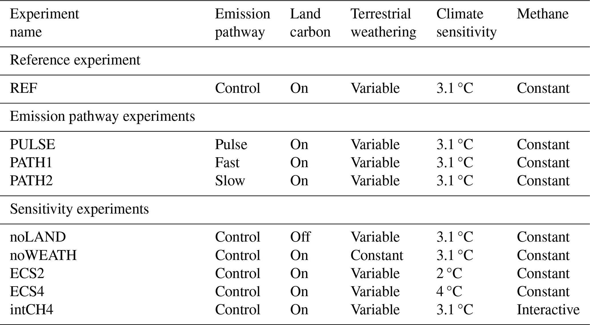
To investigate the lifetime of anthropogenic CO2 and the effect it has on the long-term evolution of the climate, we introduce idealized CO2 emission scenarios representing cumulative emissions from 0 to 5000 Pg C (Fig. E2) to cover a variety of different anthropogenic scenarios. The upper limit of ∼ 5000 Pg C has been used in many previous studies (e.g., Archer, 2005; Montenegro et al., 2007; Uchikawa and Zeebe, 2008; Archer et al., 2009a), as it just surpasses the current estimated maximum of conventional fossil fuel reserves (Lal, 2008; McGlade and Ekins, 2015). To simulate a variety of emissions pathways and explore the sensitivity of the results to the duration of the CO2 emission scenarios, we designed three different Gaussian functions with different shapes (with an increasing mean and standard deviation with higher cumulative CO2; Fig. E2) and one pulse-like perturbation where all emissions are released within the first year of the simulation. It should be noted here that the 100 kyr simulation duration includes the ramp-up and ramp-down of emissions. Following the emission function, emissions are set to 0 Pg C yr−1 for the rest of the simulation.
A number of additional experiments were performed to isolate the effect of different carbon cycle processes on the long-term fate of anthropogenic CO2. Specifically, we explored the role of the land carbon cycle response (noLAND), the impact of enabling interactive methane concentrations in the atmosphere (intCH4), and the impact of the emissions pathway (PULSE, PATH1, PATH2) on the lifetime of anthropogenic CO2. To isolate the effect of the weathering feedback on the CO2 lifetime, a dedicated set of experiments (noWEATH) was conducted in which weathering fluxes were forced to remain constant at their pre-industrial rate throughout the simulation (0.2376 Pg C yr−1 or 19.8 Tmol C yr−1 for carbonate weathering and 0.1476 Pg C yr−1 or 12.3 Tmol C yr−1 for silicate weathering). The sensitivity of the results to different equilibrium climate sensitivities (ECSs) between 2 and 4 °C was additionally investigated (ECS2, ECS4) by rescaling the equivalent CO2 in the long-wave radiation scheme (further described in Appendix A). A summary of all experimental configurations is presented in Table 1.
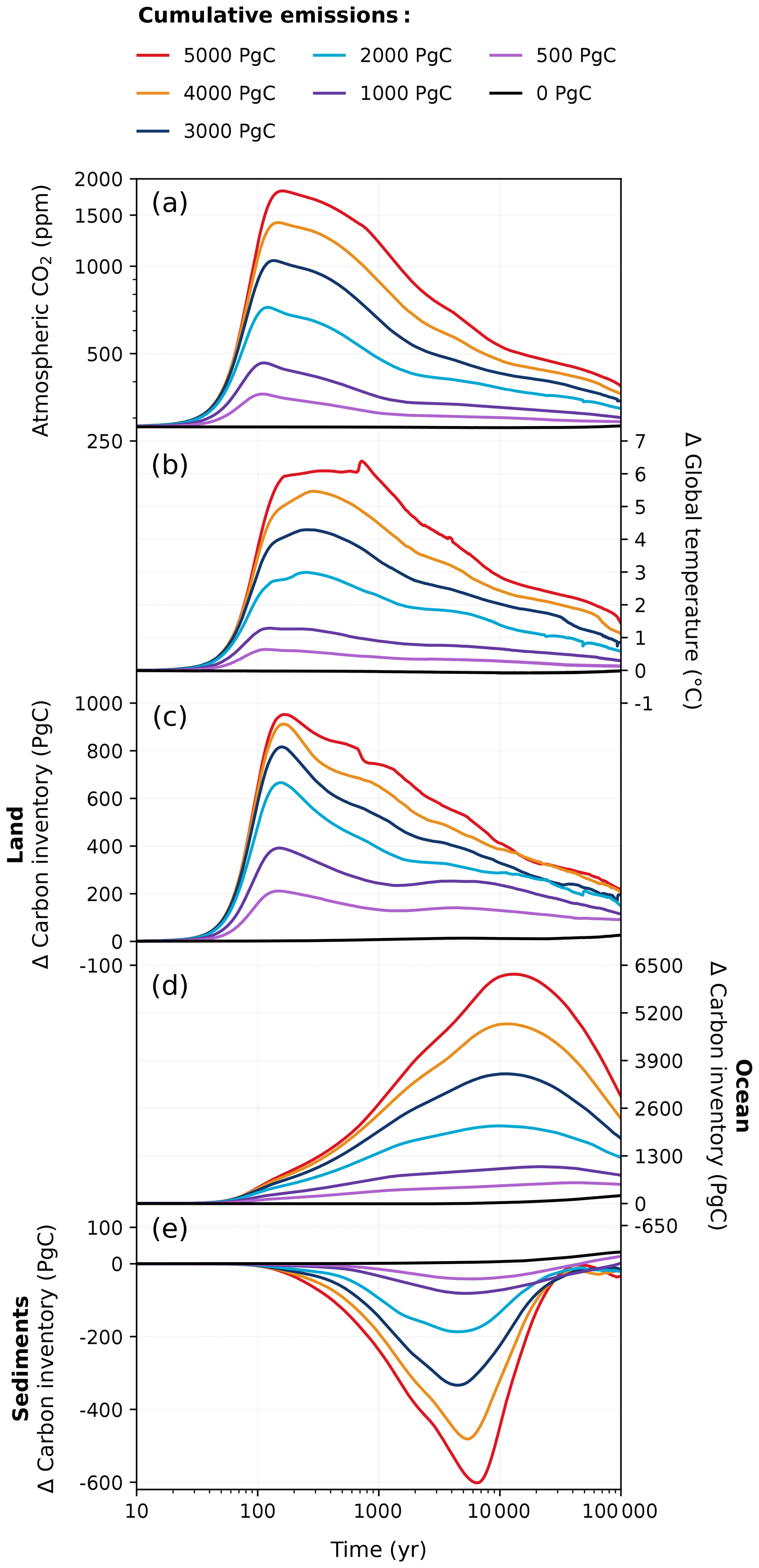
Figure 2Responses in (a) atmospheric CO2 concentration, (b) global surface air temperature, (c) land carbon inventory, (d) ocean carbon inventory, and (e) sediment carbon inventory to the full ensemble of emission scenarios (0–5000 Pg C) in the REF experiment for 100 kyr.
3.1 Long-term carbon cycle evolution
An overview of the 100 kyr atmospheric CO2 concentration and global mean temperature responses across all emission scenarios in the reference (REF) experiment can be seen in Fig. 2. The initialization of our experimental setup is demonstrably robust, evidenced by the less than 2 ppm drift (from the pre-industrial value of 280 ppm) of atmospheric CO2 concentration in the zero-emissions scenario over the span of 100 kyr (Fig. 2a). All simulations with anthropogenic emissions show a rapid increase in atmospheric CO2 concentration during the ramp-up of emissions, with peak concentrations occurring within the first 200 years. In the REF ensemble, peak CO2 concentrations fall between ∼ 360 and 1820 ppm across the different emission scenarios (Fig. 2a). These values are within the range of magnitudes reported by previous studies (e.g., Montenegro et al., 2007; Colbourn et al., 2015). We find that the increase in global mean surface temperature lags behind that of the CO2 concentration (Fig. 2b) and that the size of the temporal lag tends to increase as the cumulative emission grows (Ricke and Caldeira, 2014; Zickfeld and Herrington, 2015). Peak temperature anomalies range between ∼ 0.6 and 6.4 °C across the different emission scenarios in the REF ensemble. However, the extended decline in the Atlantic Meridional Overturning Circulation (AMOC; Fig. 7e) in the 5000 Pg C scenario results in a cooling effect in the Northern Hemisphere that prevents global mean temperature from further rising, thereby truncating peak warming. After emissions cease (∼ 150–200 years after the start of the simulation; Fig. E2), both atmospheric CO2 concentration and global temperatures decrease as carbon is taken up by the land and ocean pools (Fig. 2a–d). The only exception to this is the 5000 Pg C scenario, where there is a global temperature plateau, and global cooling is delayed until approximately ∼ 700 years after the start of the simulation, coinciding with a substantial recovery of the AMOC (Figs. 2b, 7e). Temperatures slowly decrease towards pre-industrial levels after the first millennium, and, after 10 kyr, global warming is reduced by more than half (Fig. 2b). After 100 kyr, atmospheric CO2 concentration still remains ∼ 10–100 ppm above pre-industrial levels across the different emission scenarios, and temperatures are still between ∼ 0.1 and 1.4 °C higher than the pre-industrial level at the end of the simulation.
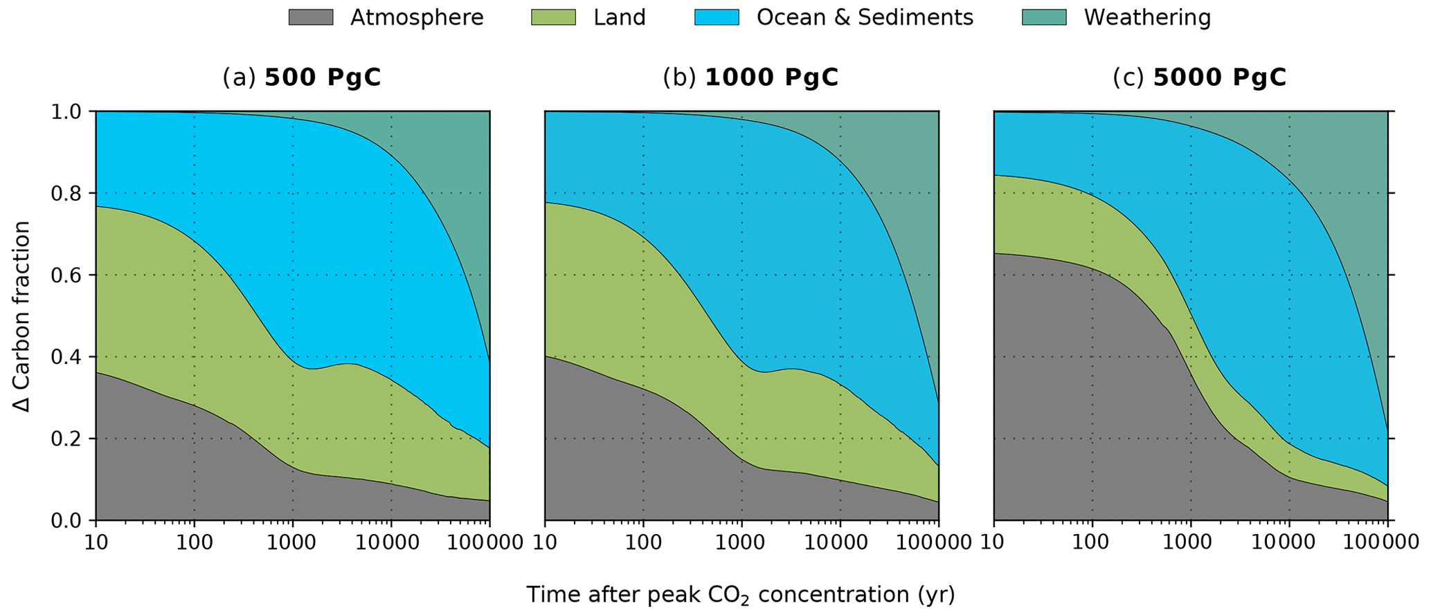
Figure 3The relative partition of anthropogenic carbon in the REF experiment after peak atmospheric CO2 concentration. The partition of the atmosphere (grey), land (green), ocean and sediments (blue), and silicate weathering (teal) is shown for the (a) 500, (b) 1000, and (c) 5000 Pg C scenarios. The calculations for these percentages is outlined in Appendix B using cumulative fluxes from the atmosphere. The carbon fraction attributed to the ocean and sediments is labelled this way, as the air–sea CO2 flux may indirectly include carbon from sediments through dissolution. However, we do not account for sediment carbon fluxes directly since there is no direct air–sediment flux (see Appendix B for further details on this formulation). It should be noted that the ramp-up of emissions is excluded here.
The fate of the anthropogenic CO2 emissions (and how this carbon is distributed among the different Earth system components) after the peak atmospheric CO2 concentration is shown in Fig. 3. The land and ocean both rapidly absorb CO2 during the ramp-up of emissions through enhanced vegetation productivity, air–sea CO2 exchange, and its subsequent dissolution (Fig. 4). At peak CO2 concentrations, the land and ocean are responsible for between 34 % and 61 % of carbon removal (19 %–39 % by land, 15 %–22 % by the ocean; Fig. 3), with the carbon removal fractions decreasing with increasing cumulative emissions. During the first 1 kyr after peak CO2 concentrations, oceanic CO2 uptake gradually slows as surface waters approach equilibrium with the atmosphere (Fig. 4b). Although the ocean carbon fraction largely increases over the first 1 kyr after peak CO2 concentrations (accounting for 46 %–59 % 1 kyr after emissions cease; Fig. 3), the carbon fraction taken up by the ocean during the latter half of the millennium appears disproportionately larger than what is taken up during the first 500 years, as land carbon has already begun decreasing by this time (Figs. 2c, 4a). Beyond the first millennium, geological processes (e.g., marine sediments and weathering) largely control the evolution of atmospheric CO2 concentration (Archer and Brovkin, 2008). Silicate weathering is responsible for 11 %–17 % of carbon removal 10 kyr after peak CO2 concentrations. However, by 100 kyr, it is responsible for the majority of carbon removal (62 %–78 %) and becomes the dominant removal process on the timescale of hundreds of thousands of years.
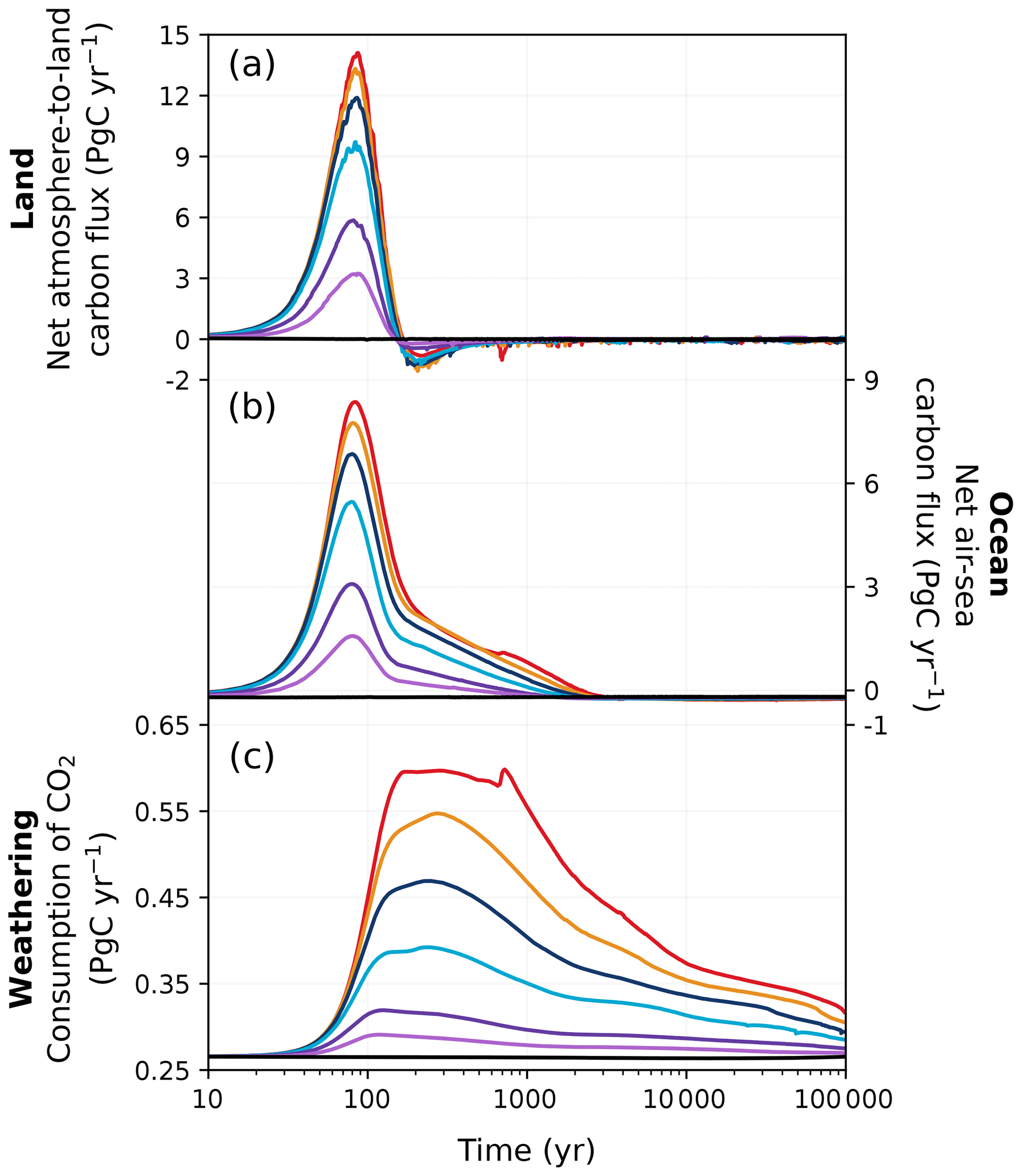
Figure 4Changes in (a) net atmosphere-to-land carbon flux, (b) net air–sea carbon flux, and (c) weathering consumption of CO2 in different emission scenarios over 100 kyr. Colours correspond to the cumulative emission scenarios shown in Fig. 2.
3.1.1 Land carbon response
Two opposing mechanisms involving vegetation and soil carbon predominantly govern the land carbon response to climate change. The land carbon pool (as the sum of vegetation and soil carbon) is initially a carbon sink due to increases in vegetation carbon (Brovkin et al., 2013), as CO2-driven fertilization enhances net primary productivity. These increases, however, can be partially or totally offset by warming-enhanced soil respiration, which strongly depends on model parameters; on whether permafrost, peatlands, and wetlands are included; and on how they are modelled in the carbon cycle model (Zickfeld et al., 2013; Eby et al., 2013). In our simulations, the peak increase in vegetation carbon significantly exceeds and more than compensates for the maximum loss in soil carbon (Fig. 5). Peak land carbon uptake in our simulations falls comfortably between the values given by previous studies (Mikolajewicz et al., 2006; Vakilifard et al., 2022).
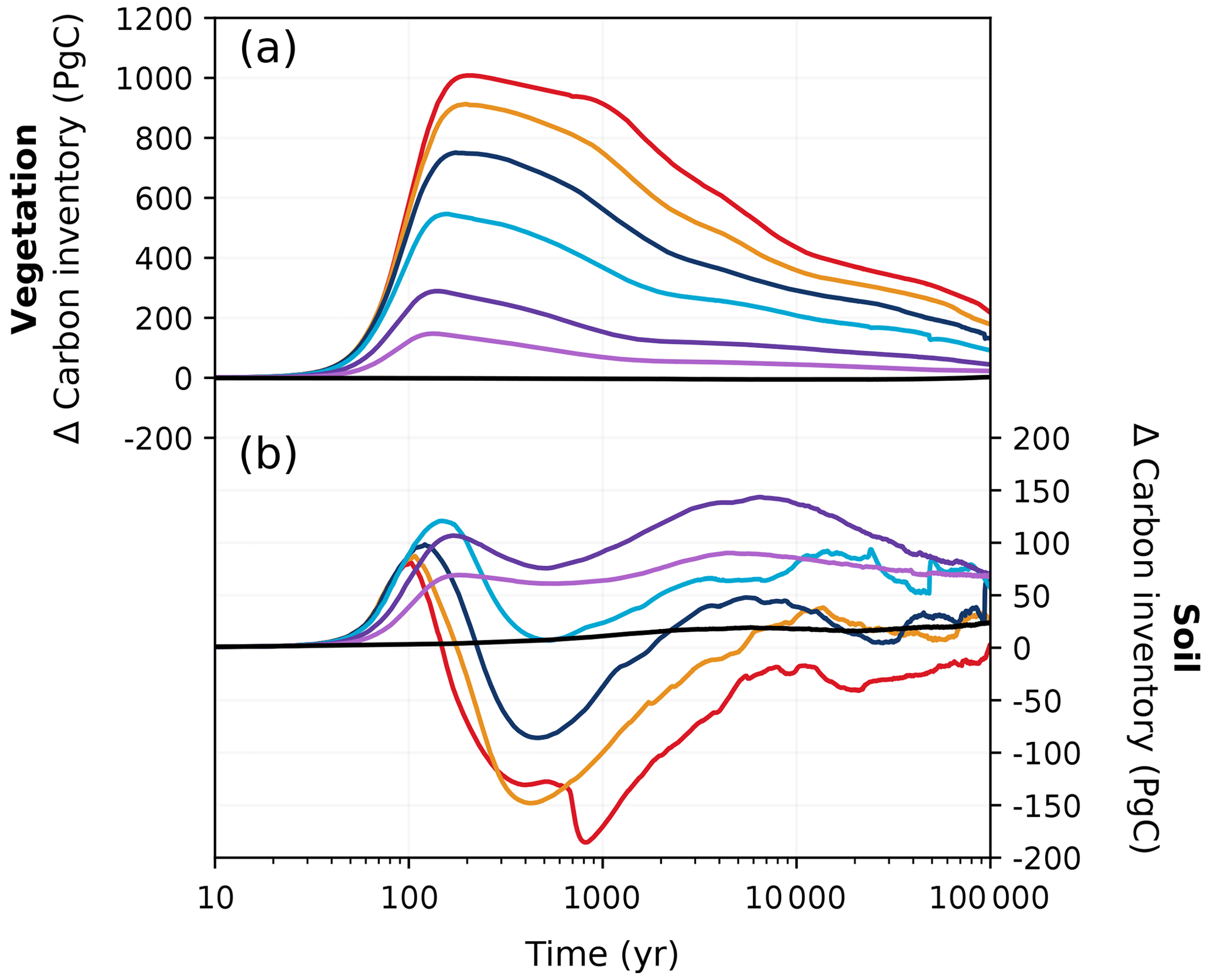
Figure 5Changes in (a) vegetation and (b) soil carbon inventories relative to the pre-industrial period in different emission scenarios over 100 kyr. Colours correspond to the cumulative emission scenarios shown in Fig. 2.
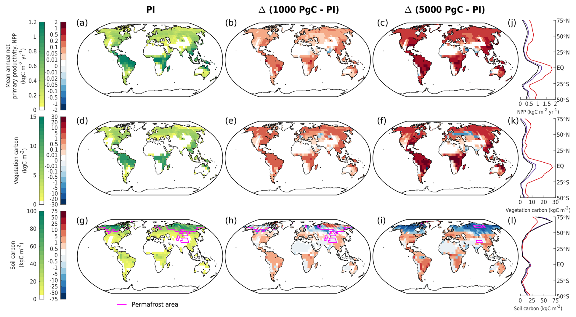
Figure 6Mean annual (a–c) net primary productivity, (d–f) vegetation carbon, and (g–i) soil carbon in different emission scenarios at 1 kyr. The columns show (a, d, g) the absolute values in the zero-emissions scenario (equivalent to the pre-industrial values), (b, e, h) the 1000 Pg C scenario relative to the pre-industrial values, and (c, f, i) the 5000 Pg C scenario relative to the pre-industrial values. Absolute values for the zonal mean are additionally shown for (j) NPP, (k) vegetation, and (l) soil carbon for the zero-emissions (black), 1000 Pg C (purple), and 5000 Pg C (red) scenarios. Magenta lines (g–i) display the permafrost area.
In the latter half of the first millennium, vegetation carbon decreases as atmospheric CO2 concentrations fall (Fig. 5a). Soil carbon exhibits non-monotonic behaviour with increasing emissions: low-emission scenarios (< 1000 Pg C) have gained up to 100 Pg C, and high-emission scenarios (> 4000 Pg C) have lost up to 150 Pg C by 1 kyr (Fig. 5b). This is because in the low-emission scenarios, the accumulation of carbon in the soil exceeds the carbon loss due to enhanced soil respiration (Fig. 6h), preventing the overall decline in soil carbon inventory (Fig. 5b). This is not the case in high-emission scenarios, as permafrost area decreases so significantly that soil respiration counteracts any potential increase when temperatures are sufficiently high (Fig. 6i). Most of the globe sees an increase in vegetation carbon with increasing emissions, mainly because of increases in net primary productivity (NPP; Fig. 6b, c, e, f). However, there are a few regions that see a decline in vegetation carbon due to a reduction in precipitation (Fig. 11h, i). Although the soil carbon inventory decreases in high-emission scenarios by 1 kyr, it recovers over the next 100 kyr as temperatures gradually decrease. In our simulations, the terrestrial storage of anthropogenic carbon is positive during the entire 100 kyr due to an increase in vegetation carbon and the recovery of soil carbon. At the end of the experiments, the land still stores approximately 7 % (range of 4 %–13 %) of the emitted anthropogenic carbon (Fig. 3).
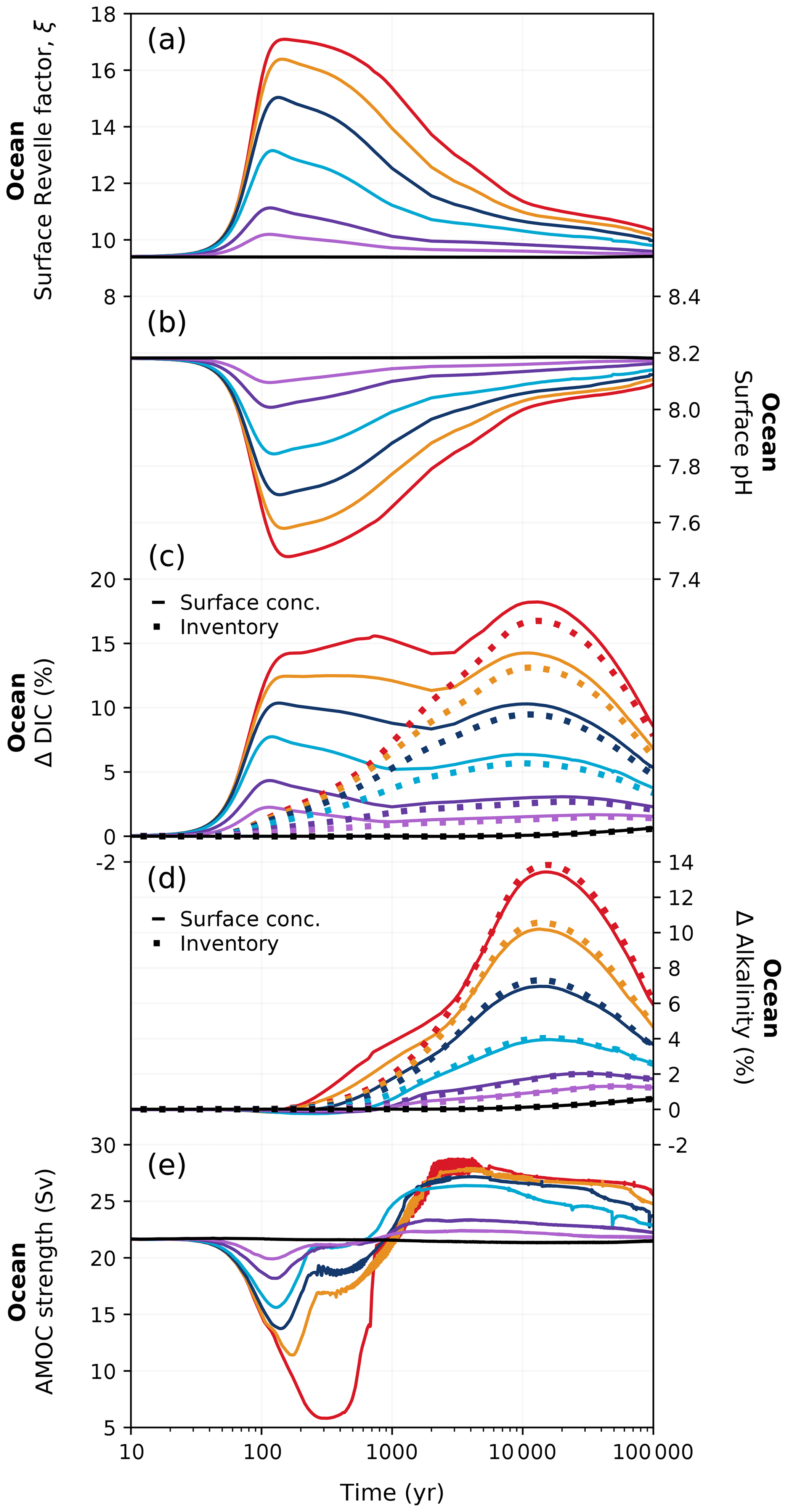
Figure 7Changes in (a) ocean buffering capacity (Revelle factor), (b) global mean surface pH, (c) relative changes in surface DIC concentration and global ocean DIC inventory, (d) relative changes in surface alkalinity concentration and global alkalinity inventory, and (e) strength of the Atlantic Meridional Overturning Circulation (AMOC) in different emission scenarios over 100 kyr. Colours correspond to the cumulative emission scenarios shown in Fig. 2. The surface ocean Revelle factor shown in (a) has been calculated via Eq. (C1) in Appendix C.
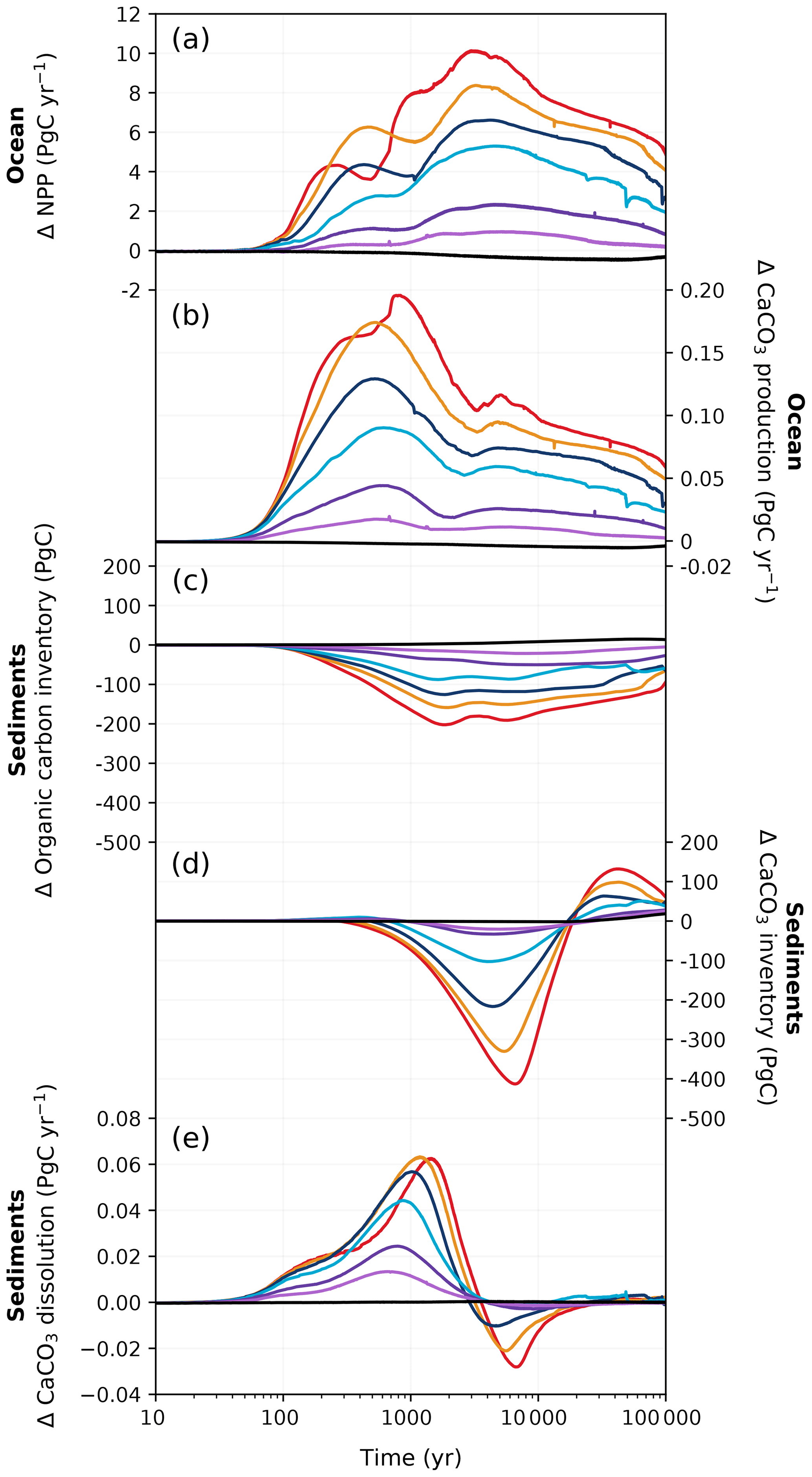
Figure 8Changes in (a) marine net primary production, (b) CaCO3 production, (c) sediment particulate organic carbon inventory, (d) sediment CaCO3 inventory, and (e) sediment CaCO3 dissolution rate in different emission scenarios over 100 kyr. Colours correspond to the cumulative emission scenarios shown in Fig. 2.
3.1.2 Ocean and sediment carbon response
The ocean absorbs and stores atmospheric CO2 due to a sequence of chemical, biological, physical, and geological processes. Under anthropogenic emissions, the ocean initially takes up carbon at an accelerated rate from greater air–sea CO2 exchange (Fig. 4b). At peak CO2 concentrations, the ocean has a net cumulative uptake between ∼ 100 and 780 Pg C depending on the emission scenario (Fig. 2d). Oceanic CO2 uptake yields bicarbonate and hydrogen ions from CO2 dissolution. As a consequence, surface ocean pH decreases at a similar rate to that which carbon is taken up in the ocean, with larger pH decreases associated with higher cumulative emissions (Fig. 7b). The magnitude of the surface ocean pH decrease in our experiments matches well with that of other studies: for example, the peak pH anomaly of approximately −0.7 in the 5000 Pg C experiment falls within the range of −0.6 to −0.8 given by other models (Caldeira and Wickett, 2005; Montenegro et al., 2007; Uchikawa and Zeebe, 2008; Eby et al., 2009; Zickfeld et al., 2012; Colbourn et al., 2015). As the phytoplankton growth rate strongly depends on temperature in HAMOCC (Ilyina et al., 2013; Willeit et al., 2023), NPP generally increases with higher sea surface temperature (SST) under larger cumulative emissions (Fig. 8a). Warming also accelerates the remineralization of organic matter in the ocean, which increases nutrient availability in the surface ocean for primary production. Moreover, reduced sea ice cover at high latitudes increases light availability and, therefore, enhances local productivity. In our highest-emission scenario, the combined effects amount to an approximate ∼ 20 % increase in peak NPP under the 5000 Pg C scenario compared to the pre-industrial value (53.3 Pg C yr−1; Fig. 8a).
As the amount of dissolved CO2 in the surface ocean rises, its ability to absorb excess CO2 decreases. This decrease in buffering capacity is illustrated by the Revelle factor (ξ, the sensitivity of pCO2 to changes in DIC; Revelle and Suess, 1957), which increases with higher emissions (Fig. 7a). The pre-industrial Revelle factor of ∼ 9.4 matches reasonably well with that calculated by Jiang et al. (2019), and the peak Revelle factor in the 500 Pg C scenario (∼ 10.2) is close to that calculated using present-day GLODAPv2 observations (Terhaar et al., 2022). Between 100 years and 1 kyr, ξ slowly decreases owing to the gradual decrease in surface DIC (except for the 5000 Pg C scenario, Fig. 7c) and the increase in surface alkalinity (Fig. 7d). The decrease in surface DIC results from the combined effect of the downward transport of anthropogenic carbon in the surface ocean and the enhanced biological production (Fig. 8a), which is partly counteracted by the increase in the global DIC inventory (Fig. 7c). Both DIC and alkalinity inventories increase during this period due to high carbonate weathering fluxes (input as into the ocean; see Fig. 9a) and enhanced refluxes from sediment. Although NPP increases with warming, the loss of organic carbon to the sediment (not shown) and the organic carbon content in the sediment (Fig. 8c) are reduced due to higher remineralization rates in both the water column and sediment. Deep convection, which transports surface waters with decreased pH and carbonate ion concentrations into the interior ocean, together with increased organic matter remineralization, causes carbonate ion concentrations in the interior ocean to fall with increasing emissions (Fig. E5). In response, the lysocline and carbonate compensation depth (CCD) shoal and sediment CaCO3 dissolves (contributing more to the total loss of the sediment carbon inventory than sediment organic carbon does; Fig. 2e), driving the increase in the alkalinity inventory. In the 5000 Pg C scenario, surface DIC increases between the years 1100 and 1700, which is likely due to the extended period of the AMOC decline (Fig. 7e) that inhibits deep convection and downward carbon transport.
Surface DIC shows diverse variations between 1 and 10 kyr depending on the emission scenario, whereas surface alkalinity generally increases and is responsible for the recovery of the buffering capacity (shown by the continuous decline in ξ). The variation in surface alkalinity generally follows that of the global inventory, with the latter controlled by the weathering input and the net loss to the sediment. The sediment CaCO3 continues to dissolve at a higher rate than in the first millennium (Fig. 8e). Beyond 10 kyr, both surface DIC and alkalinity decline following the global inventory as a response to decreased carbonate weathering (Fig. 9a) and increased loss to the sediment (Fig. 8c, d). Due to silicate weathering (Sect. 3.1.3), which reduces atmospheric CO2, the ocean becomes a carbon source, contributing to the decrease in surface DIC and the recovery of the buffering capacity. The impact of carbonate compensation and seafloor CaCO3 neutralization on the restoration of the buffering capacity on the millennial timescales shown in these simulations is in line with previous studies (Archer et al., 1997, 1998; Tyrrell et al., 2007a; Tyrrell, 2007b). The recovery of the sediment CaCO3 inventory occurs roughly around the same time as that predicted by Lenton and Britton (2006). However, the timing of peak CaCO3 dissolution in CLIMBER-X is earlier than in a CLIMBER-2 study by Montenegro et al. (2007), which may be due to increased biological production of CaCO3 (as it is proportional to organic detritus production and, thus, NPP; Fig. 8a) leading to more CaCO3 export to the interior ocean.
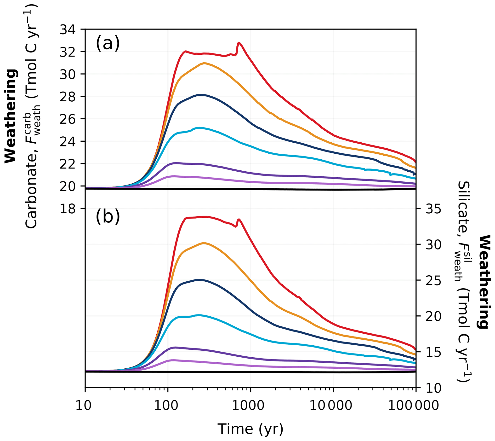
Figure 9Changes in (a) carbonate and (b) silicate weathering fluxes in different emission scenarios over 100 kyr. Colours correspond to the cumulative emission scenarios shown in Fig. 2.
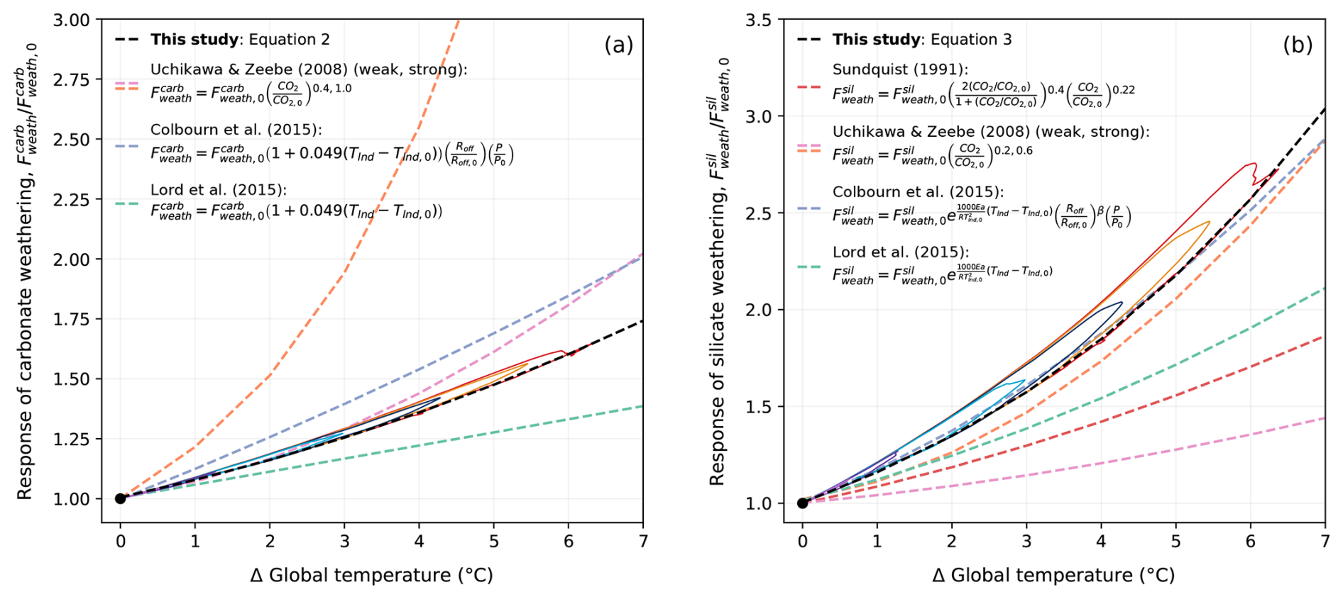
Figure 10Relationship between (a) carbonate weathering, (b) silicate weathering, and temperature in previous studies and CLIMBER-X. Solid coloured lines corresponding to the cumulative emission scenarios seen in Fig. 2 represent the weathering response in the REF ensemble. The dashed black lines in (a) and (b) show an exponential fit of the trajectory of the weathering response. Calculated trajectories have additionally been plotted for the equations used by Sundquist (1991), Uchikawa and Zeebe (2008), Colbourn et al. (2015) (with runoff, Roff, and productivity, P, parametrized as a function of CO2, as in Colbourn et al., 2013), and Lord et al. (2015b) specifically using CLIMBER-X variables for atmospheric CO2 (CO2) and land surface temperature (Tlnd). The fit of these trajectories has been plotted above using Numpy.Polyfit in Python. It should be noted that since this comparison is based on the simulated CLIMBER-X variables, it implicitly assumes an ECS of 3.1 °C.
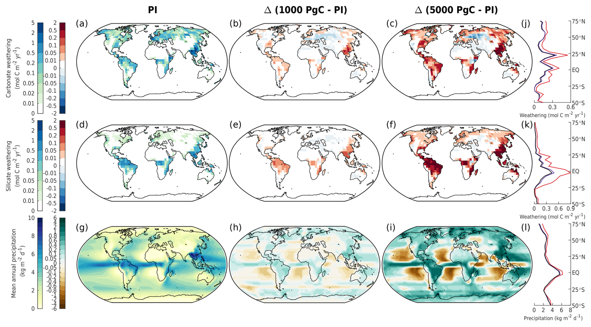
Figure 11Mean annual (a–c) carbonate weathering, (d–f) silicate weathering, and (g–i) precipitation in different emission scenarios at 1 kyr. The columns show (a, d, g) the absolute values in the zero-emissions scenario (equivalent to the pre-industrial values), (b, e, h) the 1000 Pg C scenario relative to the pre-industrial values, and (c, f, i) the 5000 Pg C scenario relative to the pre-industrial values. Absolute values for the zonal mean are additionally shown for (j) carbonate weathering, (k) silicate weathering, and (l) precipitation for the zero-emissions (black), 1000 Pg C (purple), and 5000 Pg C (red) scenarios.
3.1.3 Weathering response
While the pre-industrial weathering fluxes in our simulations (19.8 Tmol C yr−1 for carbonate and 12.3 Tmol C yr−1 for silicate; Fig. 9) fall within but toward the higher end of observational estimates (Meybeck, 1987; Gaillardet et al., 1999; Munhoven, 2002; Amiotte Suchet et al., 2003), they are significantly higher than previous studies investigating the long-term future CO2 evolution (Uchikawa and Zeebe, 2008; Colbourn et al., 2015; Lord et al., 2015b). This is at least partly due to the spatially explicit weathering scheme employed in our model, as switching from a 0D to a 2D scheme has been shown to increase global weathering rates (Colbourn, 2011; Colbourn et al., 2013). Chemical weathering on land increases in high-emission scenarios due to warmer and wetter conditions, drawing down more carbon from the atmosphere (Fig. 9). Both carbonate and silicate weathering rapidly increase over the first 200 years as a response to elevated temperatures and increased runoff (Lenton and Britton, 2006). The carbonate weathering flux increases to 20.8–32.0 Tmol C yr−1 in the different scenarios around the same time as the peak atmospheric CO2 concentration (Fig. 9a). Peak silicate weathering occurs at the same time but has even larger differences from the pre-industrial value, nearly tripling under the high-emission scenario (Fig. 9b). After peak weathering fluxes are reached in the REF ensemble, they begin to decrease within the first millennium as atmospheric CO2 decreases.
The sensitivity of carbonate and silicate weathering to climate change in CLIMBER-X is compared to estimates from earlier investigations in Fig. 10a, b. Generally, the CLIMBER-X response falls between those estimated by previous studies (Sundquist, 1991; Uchikawa and Zeebe, 2008; Colbourn et al., 2015; Lord et al., 2015b), with the response of carbonate weathering falling in the middle and silicate weathering tending to be on the stronger side. In both cases, however, the weathering response is higher than was simulated by the equations used in Lord et al. (2015b). In addition to this, the more sophisticated weathering scheme in CLIMBER-X produces a narrow hysteresis in the response to the change in global mean temperature (Fig. 10a, b), as weathering fluxes decrease more slowly than global mean temperature does. This hysteresis is primarily due to a lag between the evolution of precipitation and temperature. The combination of a rather large pre-industrial silicate weathering flux and high sensitivity of silicate weathering to climate in the model results in a weathering feedback that is stronger than in some previous studies (Lord et al., 2015b; Colbourn et al., 2015). This has implications for the lifetime of atmospheric CO2 (Sect. 3.2).
Most previous studies on deep-future CO2 concentrations did not spatially resolve weathering, instead relying on global mean values. The few studies that did use spatially explicit weathering employed either the GKWM (Bluth and Kump, 1991) or GEM-CO2 (Amiotte Suchet et al., 2003) lithological maps, which have quite coarse resolutions compared to the GLiM (Hartmann, 2009a) lithological map used by CLIMBER-X. The pre-industrial carbonate and silicate weathering distributions are shown in Fig. 11a, d. These distributions align quite closely with the calculated distribution of CO2 consumption from Hartmann et al. (2009b). However, not all details can be reproduced, given the 5°×5° resolution of CLIMBER-X and biases in precipitation (Fig. 11g; see Willeit et al., 2022). Weathering rates rise with increasing temperature, particularly in regions where significant weathering is already taking place. Runoff, which indirectly depends on precipitation through soil infiltration and drainage (Willeit and Ganopolski, 2016), drives some of these changes (Figs. 11g, h, i, E6). As emissions grow, silicate weathering sees a significant increase in the tropical rain belt area due to higher precipitation. These include regions such as Southeast Asia, central Africa, and Brazil (Fig. 11k). Large changes in carbonate weathering are more globally distributed than silicate weathering (Fig. 11e, f). However, like silicate weathering, large changes in carbonate weathering (e.g., increases and decreases in carbonate weathering in Southeast Asia and central Asia compared to the pre-industrial values) can also be explained by increases and decreases in precipitation (Fig. 11b, c). Such spatial patterns in silicate and carbonate weathering under idealized 1000 and 5000 Pg C scenarios have also been seen by Brault et al. (2017). In our simulations, highly active weathering regions are dominant contributors to the global weathering flux. About 10 % of land area across the different emission scenarios is responsible for ∼ 13 %–14 % of the total carbonate weathering and ∼ 33 %–37 % of the total silicate weathering (Fig. 11b, c, e, f). Given that the simulated weathering rates for both carbonate and silicate rocks are quite spatially heterogeneous, simplifications used by previous studies to calculate weathering rates (e.g., weathering as a function of global mean land surface temperature) could be insufficient to describe the feedback between climate and weathering.
3.2 Atmospheric lifetime of anthropogenic CO2
The atmospheric lifetime of anthropogenic CO2 across the different scenarios is estimated using an impulse response function (IRF). This is a first-order approximation of the long-term effects of a short-term perturbation. It can be applied to changes in atmospheric CO2 concentration (normalized by cumulative CO2 emissions) such that it represents the fraction of emissions remaining (Maier-Reimer and Hasselmann, 1987; Joos et al., 2013; Jeltsch-Thömmes and Joos, 2020). In this formulation, it is functionally no different than the airborne fraction, but we distinguish between the two by assuming that the IRF is only valid for times after the peak CO2 concentration (CO). This can be written as the following equation:
where E is cumulative emissions in Pg C, ΔCO2(t) is the change in atmospheric CO2 concentration at time t compared to the pre-industrial concentration (280 ppm), and 2.214 Pg C ppm−1 is the conversion factor between concentration and mass (Friedlingstein et al., 2023). The IRF for the REF ensemble is shown in Fig. 12a, c. The ramp-up of emissions is not included in this analysis. Unlike previous studies (e.g., Archer et al., 2009a; Joos et al., 2013), we do not deploy an instantaneous pulse in the REF ensemble, and our fractions of emissions remaining do not start at 1, as carbon sequestration began during the ramp-up of emissions. While it is unlikely that the emissions pathway will be an important factor for the atmospheric lifetime on long timescales, the IRF for the PULSE, PATH1 and PATH2 ensembles has additionally been plotted in Fig. 12b to explicitly show the impact of the emissions pathway. Although the emissions pathway has a notable impact on the IRF within the first millennium, this effect becomes largely negligible after ∼ 3 kyr. This supports the long-term path independence found by Zickfeld et al. (2012) and Herrington and Zickfeld (2014), meaning that despite the potential complication from the ramp-up and ramp-down periods of emissions in the REF experiment, our results are fully comparable with those in the Long-Term Model Intercomparison Project (LTMIP) in Archer et al. (2009a).
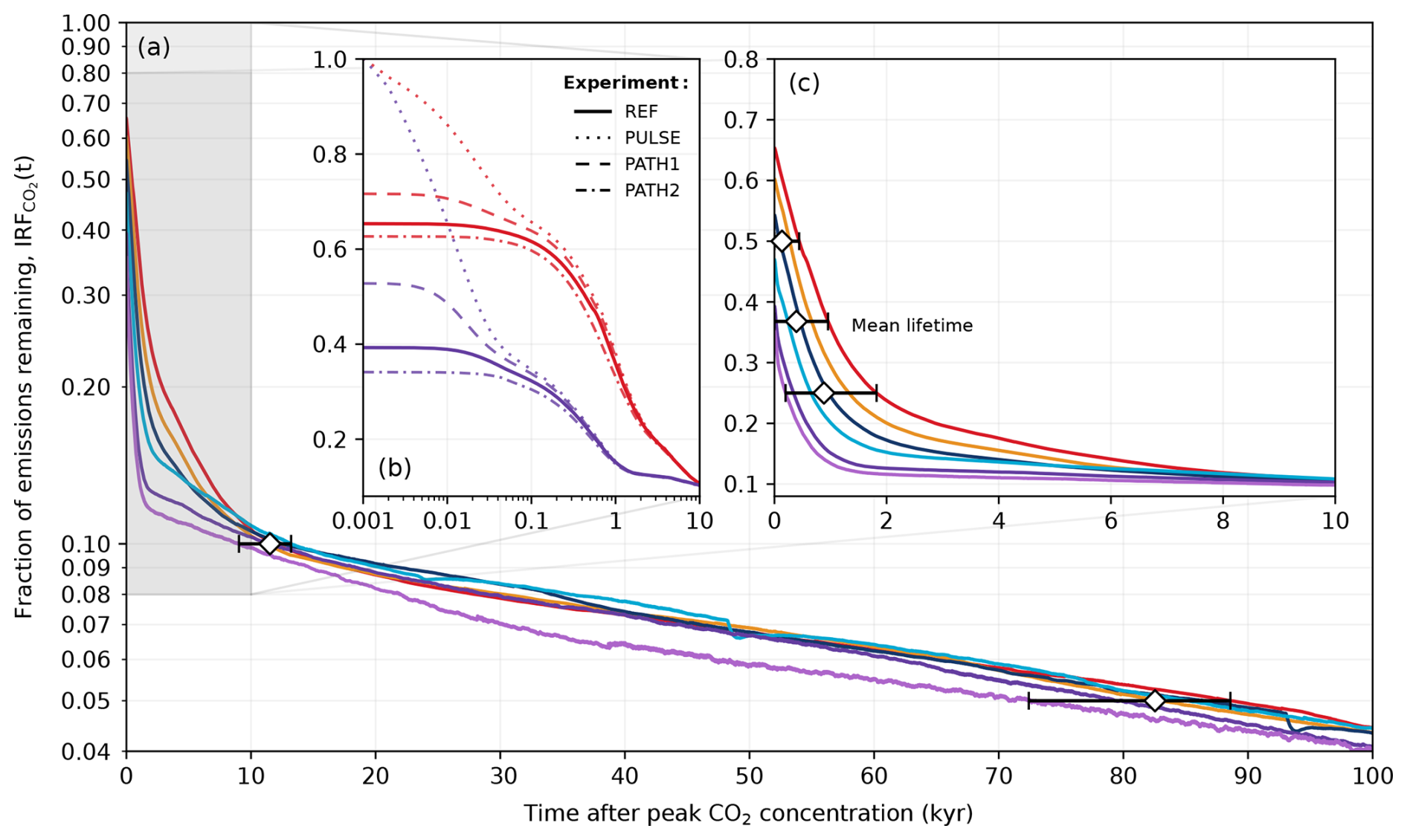
Figure 12Atmospheric lifetime of anthropogenic CO2 described by IRF(t). Colours correspond to the cumulative emission scenarios shown in Fig. 2. (a) Fraction of emissions remaining in the atmosphere after peak CO2 concentration for the different emission scenarios in the REF experiment. (b) Fraction of emissions remaining in the atmosphere over the first 10 kyr after peak CO2 concentration. Here, the x axis is log-scaled and only shows the 1000 Pg C (purple) and 5000 Pg C (red) scenarios. The PULSE, PATH1, and PATH2 experiments have additionally been plotted to show the effect of the emissions pathway on the IRF. (c) Same as (a) but for the first 10 kyr after peak CO2 concentration. The diamond markers and horizontal bars represent the mean time and spread in which the different emission scenarios reach 50 %, ≈ % (mean lifetime), 25 %, 10 %, and 5 % of their original cumulative emissions.
Modelling studies have suggested that the majority (up to 80 %) of anthropogenic CO2 is quickly taken up by fast carbon processes, leading to a mean lifetime of only a few centuries (Archer, 2005; Montenegro et al., 2007; Archer and Brovkin, 2008). In the REF ensemble, the mean lifetime is 390 (range of 0–955) years (Fig. 12c). This value depends on the cumulative emission load to the atmosphere (Fig. 12c) and, to some extent, the pathway of the emission (Fig. 12b). This explains why the lifetime determined by the timing of IRF is close to zero in the 500 Pg C scenario, as the majority of the carbon is taken up from the atmosphere prior to reaching the peak atmospheric CO2 concentration in our simulations (Fig. 3c). On average, it takes between 197 and 1820 years after peak CO2 concentration to remove 75 % of anthropogenic emissions, depending on the emission scenario. Our results (Fig. 12c) generally agree with the most comprehensive assessment to date, which indicates that between 20 % and 35 % of CO2 remains in the atmosphere after 200–2000 years (Archer et al., 2009a). After 10 kyr, it has been previously reported that CO2 emissions in the atmosphere would remain somewhere between ∼ 5 % and 20 % for the 1000 Pg C scenario and ∼ 10 % and 35 % for 5000 Pg C scenario (Archer et al., 2009a). In all experiments, the atmospheric CO2 concentration has decreased to approximately 10 % of its initial value after 10 kyr across the different emission scenarios (Fig. 12c). Our values are on the lower end of the range provided by Archer et al. (2009a) due to the combined effect of a higher pre-industrial weathering rate and stronger weathering feedbacks. After 100 kyr from the start of the REF experiments, the fraction of emissions remaining is on average 4.3 % (range of 4.0 %–4.4 %) across the different emission scenarios (Fig. 12a). This falls in between estimates by previous studies, which have reported that between 2 % and 7 % of emissions will remain in the atmosphere beyond 100 kyr (Archer, 2005; Lenton and Britton, 2006; Jeltsch-Thömmes and Joos, 2020).
3.3 Multi-exponential timescale analysis
We conducted a least-squares fit of a multi-exponential decay function to tease out different timescales that can otherwise be associated with long-term processes that take up excess CO2. This analysis was exclusively done on the REF ensemble, the ensemble with a pulse-like perturbation of CO2 (PULSE; Table 1), and the ensemble with land carbon disabled (noLAND; Table 1). The latter two experiments were included to (1) provide confidence in our estimated timescales by excluding the ramp-up period of emissions as a factor (aligning with the procedure used in similar studies, e.g., Archer et al., 1997) and (2) facilitate a direct comparison with the findings of Lord et al. (2015b). The Python function curve_fit in Scipy.Optimize was used, employing nonlinear least squares to fit the following function to our data:
where CO2(t) is the CO2 concentration at time t (where CO), and is the peak CO2 concentration compared to the pre-industrial concentration (280 ppm). This function represents the superposition of exponential decay functions each with their own time constant, τi, and amplitude, Ai (Maier-Reimer and Hasselmann, 1987). Here, the former represents the timescale of decay (i.e., the removal timescale) and the latter represents the fraction of emissions removed over that timescale. Since an instantaneous emission pulse was not used in the REF and noLAND experiments, the first ∼ 200 years of our simulations were dedicated to the ramp-up and ramp-down of atmospheric CO2 concentrations (Fig. E2). Therefore, we decided to fit all data starting from the peak concentration in atmospheric CO2 (as done in Sect. 3.2), thereby omitting the ramp-up period of emissions. Several superimposed exponential functions were used to fit the data (from n=1 to 6), but fast convergence times and significantly high (> 0.97) R2 values were found for n=3.
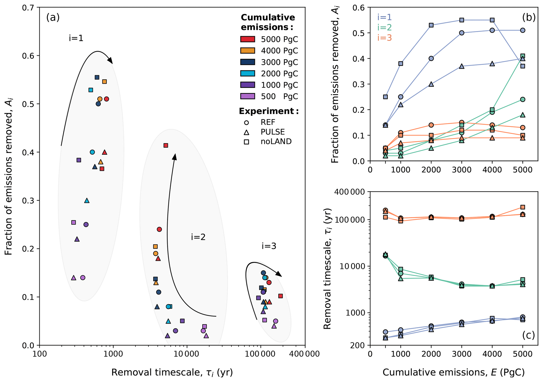
Figure 13Dependence of fitting parameters (Ai and τi) determined in the multi-exponential decay analysis of CO2 concentration in the REF, PULSE, and noLAND experiments. Different markers have been used to convey different experiments. The arrows in (a) indicate how the ability of individual processes to remove anthropogenic CO2 changes as total emissions increase. This is shown more explicitly in (b) and (c), which depict how the fraction of emissions remaining and the removal timescales for different processes change with increasing emissions. Scenarios with smaller cumulative emissions typically result in lower Ai values, as a larger proportion of emissions is taken up by short-term processes (sub-centennial timescales), which are not considered in our multi-exponential fitting procedure (see Lord et al., 2015b).
We should first highlight the fact that it is not surprising that n=3 yielded a good fit across the different experiments. Although the equilibrium timescales for fast carbon processes have been thoroughly examined in the literature previously (e.g., Eby et al., 2009), Archer and Brovkin (2008) showed that long-term carbon uptake is predominately controlled by the slow processes of (1) ocean invasion, (2) reactions with CaCO3, and (3) reactions with igneous (i.e., silicate) rocks. In some studies, these are sometimes more broadly grouped into ocean and geological processes, with CaCO3 reactions further split into sea floor and terrestrial CaCO3 neutralization (corresponding to n=4, e.g., Archer et al., 1997). Other studies have used higher orders of n to account for (or further break down) processes related to land carbon, air–sea CO2 exchange, ocean invasion, carbonate chemistry, mixed-layer mixing, and deep-ocean mixing (Colbourn et al., 2015; Lord et al., 2015b; Jeltsch-Thömmes and Joos, 2020). Short-term processes (i.e., sub-centennial timescales) cannot be fit for the REF and noLAND experiments, given potential complications with and the removal of the ramp-up period. However, n=3 is already sufficient to examine the long-term uptake of anthropogenic CO2. It should be noted that due to this decision, the values for Ai in the REF, PULSE, and noLAND experiments do not sum to 1 (Fig. 12b). This is because for the REF and noLAND experiments, a fraction of emissions was already removed via short-term processes during the excluded ramp-up period. A more accurate fit could be achieved for the PULSE experiment by increasing the number of fitted exponentials; however, we kept n=3 to maintain consistency in our analysis. In the REF ensemble, removal timescales of 386–810 years for i=1, ∼ 4–17 kyr for i=2, and ∼ 108–159 kyr for i=3 were found across the different emission scenarios (Table E2). The estimated range of removal timescales marginally changes for the PULSE and noLAND experiments (Table E2).
The centennial magnitude of the first removal timescale (i=1) suggests the involvement of ocean circulation, which we interpret as the deep-ocean processes responsible for transporting CO2 away from the surface. The range determined in the REF, PULSE, and noLAND experiments fits well within previous estimates: for example, Archer et al. (2009a) found a range of 250–450 years, while Lord et al. (2015b) found 230–880 years. The ability of this process to remove carbon with increasing emissions is nonlinear, as the fraction of emissions removed steadily increases until ∼ 3000–4000 Pg C of cumulative emissions (Fig. 13b). A major cause of this behaviour is the slowdown of ocean circulation during the first millennium, as seen by the weakening of the AMOC. In our experiments, both the duration and magnitude of the AMOC weakening increase with larger cumulative emissions (Fig. 7e), followed by a subsequent strengthening of the AMOC after emissions cease, which overshoots the pre-industrial value. This promotes the downward transport of anthropogenic carbon and therefore increases the oceanic carbon uptake capacity (Montenegro et al., 2007; Lord et al., 2015b). In the 5000 Pg C scenario, however, the behaviour of this timescale differs significantly between the three experiments (Fig. 13). While deep-ocean processes in the REF (and to some extent, in the PULSE) experiment stabilize at a similar removal capacity as in the 4000 Pg C scenario (Table E2), its ability to remove carbon is notably reduced in the noLAND experiment (∼ 37 %). In the REF experiment, the AMOC does not begin to recover until 200–300 years after emissions end in the 5000 Pg C scenario (Fig. 7e), leading to large amount of anthropogenic carbon accumulating in the upper ocean by 1 kyr (Fig. E3). However, the AMOC eventually recovers and follows a similar trajectory to that of the 4000 Pg C experiment. This is also true for the PULSE experiment, although not shown. Meanwhile, the AMOC fails to recover at 5000 Pg C in the noLAND experiment, shutting down for the majority of the simulation (not shown). This results in the decreased ability of deep-ocean processes to absorb additional anthropogenic CO2.
Previous studies have given a range of 1–6 kyr for sediment dissolution and 6–14 kyr for carbonate weathering (Sundquist, 1991; Archer et al., 1997; Ridgwell and Hargreaves, 2007; Colbourn et al., 2015; Lord et al., 2015b; Jeltsch-Thömmes and Joos, 2020). However, it has been emphasized that these processes should not be considered separately, given their interdependence (Lord et al., 2015b). We attribute the second calculated timescale (i=2), which is similar in all three experiments and falls within the estimated range, to the combined influence of both processes. As emissions increase to 4000 Pg C, the removal timescale shortens (Fig. 13c), and a higher fraction of emissions is removed (Fig. 13b). The enhanced ability of this timescale to remove anthropogenic CO2 with larger cumulative emissions is primarily driven by the resulting increase in carbonate weathering, which leads to more in the ocean (Fig. 9a). In low-emission scenarios, the calculated removal timescale is closer to ∼ 17 kyr, suggesting that the terrestrial weathering of carbonate rocks is the dominant process of carbon removal. But considering the fact that this timescale generally has a limited capacity to remove additional anthropogenic CO2 (∼ 3 %–4 % in the REF ensemble; Table E2), it suggests that the combined effect of enhanced carbonate weathering (Fig. 9a) and CaCO3 dissolution (Fig. 8e) is relatively weak in low-emission scenarios.
In high-emission scenarios, however, the timescale shortens to about 4 kyr, closer to that estimated for marine sediment dissolution. Sediment dissolution from a shoaling lysocline and CCD in the 3000–5000 Pg C scenarios reaches a similar maximum of ∼ 0.17 Pg C yr−1 shortly after the first millennium in the REF experiment (Fig. 8e). As this process restores buffering capacity to the ocean and is responsible for the continued removal of anthropogenic CO2, it is perhaps not so surprising that there is a discernible threshold in the removal timescale at these levels of emissions. Again, the removal ability of this timescale in the 5000 Pg C scenario differs significantly between the REF, PULSE, and noLAND experiments. This scenario in the noLAND ensemble accounts for the removal of nearly twice as much anthropogenic CO2 compared to the other two (41 % vs. 18 % and 24 %). This shows that a weakening ability of deep-ocean processes to take up CO2 is compensated by an increasing ability of sediment dissolution, to some extent (similarly shown in Archer et al., 1997), and is because seafloor CaCO3 neutralization will act to restore the buffering capacity that has been depleted from highly alkaline deep water (Fig. E4c, g, k).
The last timescale to be considered (i=3) pertains to silicate weathering. The multi-exponential analysis shown here provides an estimate of the silicate weathering timescale that is significantly shorter than what has been previously reported. For the first time, a non-monotonic dependence of the silicate weathering timescale and capacity for carbon removal of cumulative emissions were found. This trend is seen in the REF, PULSE, and noLAND experiments, although the spread of the timescale significantly changes between the different experiments. In the 500 Pg C scenario, silicate weathering is responsible for removing ∼ 4 %–5 % of anthropogenic CO2 across the different experiments (Table E2). However, the removal timescale is approximately 159 kyr in the REF ensemble, 151 kyr in the PULSE ensemble, and 113 kyr in the noLAND ensemble – the latter nearly a factor 2 smaller than originally estimated by Archer et al. (1997), Colbourn et al. (2015), and Lord et al. (2015b). The ability of this process to remove carbon increases up to a maximum of 15 % (seen in the REF ensemble) as emissions increase. At the same time, the removal timescale of silicate weathering in the REF ensemble decreases to ∼107 kyr in the 1000 Pg C scenario before generally increasing to ∼ 129 kyr in the 5000 Pg C scenario (Fig. 13c). This trend can also be seen in the PULSE and noLAND experiments (Fig. 13c). The initial shortening of the silicate weathering timescale with increasing emissions can be partially explained by spatially explicit weathering (Colbourn et al., 2013) and strong weathering feedbacks (Sect. 3.1). This is not unexpected, given that differences in weathering parametrizations have been found to change the estimated timescale of silicate weathering by more than 100 kyr (Uchikawa and Zeebe, 2008; Colbourn et al., 2015).
The behaviour of the silicate weathering timescale mirrors that of CaCO3 reactions, as the timescale generally decreases as emissions rise until approximately 3000–4000 Pg C (Fig. 13c). The threshold of ∼ 3000–4000 Pg C is also seen for deep-ocean processes, which increase in removal ability until that point (Fig. 13b). The non-monotonic behaviour of the silicate weathering timescale and carbon removal ability can be attributed to the same physical mechanisms responsible for the nonlinearity observed in deep-ocean processes and CaCO3 reactions. If the removal by either of these processes is strong, it can diminish the effectiveness of silicate weathering by reducing the amount of atmospheric CO2 available for it to act upon. As such, the AMOC likely plays a significant role in the removal timescale of silicate weathering, as experiments with a delayed AMOC recovery (Fig. 7e) or a complete shutdown (not shown) show an increase in the timescale. Since emission scenarios greater than 5000 Pg C were not explored, it is unclear whether this trend will continue with increasing emissions. Despite differences in our estimated timescale of silicate weathering, the ability of silicate weathering to remove carbon (∼ 4 %–15 % across all experiments and scenarios; Table E2) falls reasonably close to that of previous studies, which have reported values between 4 % and 10 % (Lenton and Britton, 2006; Ridgwell and Hargreaves, 2007; Archer, 2005; Colbourn et al., 2015; Lord et al., 2015b).
3.4 Continuum of removal timescales
The multi-exponential decomposition of atmospheric CO2 (Sect. 3.3) is, to some extent, dependent on how well a discrete number of functions can describe the continuous decline in atmospheric CO2. This drawback has been recognized and discussed by other studies (e.g., Jeltsch-Thömmes and Joos, 2020). Therefore, we have derived an alternative method to calculate the removal timescale of anthropogenic CO2 emissions as a function of time. With this method, the following first-order exponential decay equation describing the decline in atmospheric CO2 (Eq. 6) is solved to estimate the removal timescale, τ(t). This was done by estimating the derivative using a central-difference approach:
where ΔCO2(t) is the change in atmospheric CO2 concentration at time t (where CO) compared to the pre-industrial concentration (280 ppm). In doing this, the time-dependence of the calculated removal timescales was examined, along with how it changes for different levels of cumulative CO2 emissions. We employed a rolling mean with an increasing window size over time such that larger removal timescales are averaged over longer time periods. This has been more thoroughly described in Appendix D. As in the procedures in Sect. 3.2 and 3.3, the ramp-up period of emissions was excluded, meaning that this analysis was carried out for data after the peak CO2 concentration had been reached (CO). This method was conducted exclusively on the REF ensemble, as one of its objectives was to provide greater confidence in the results obtained from Sect. 3.3.
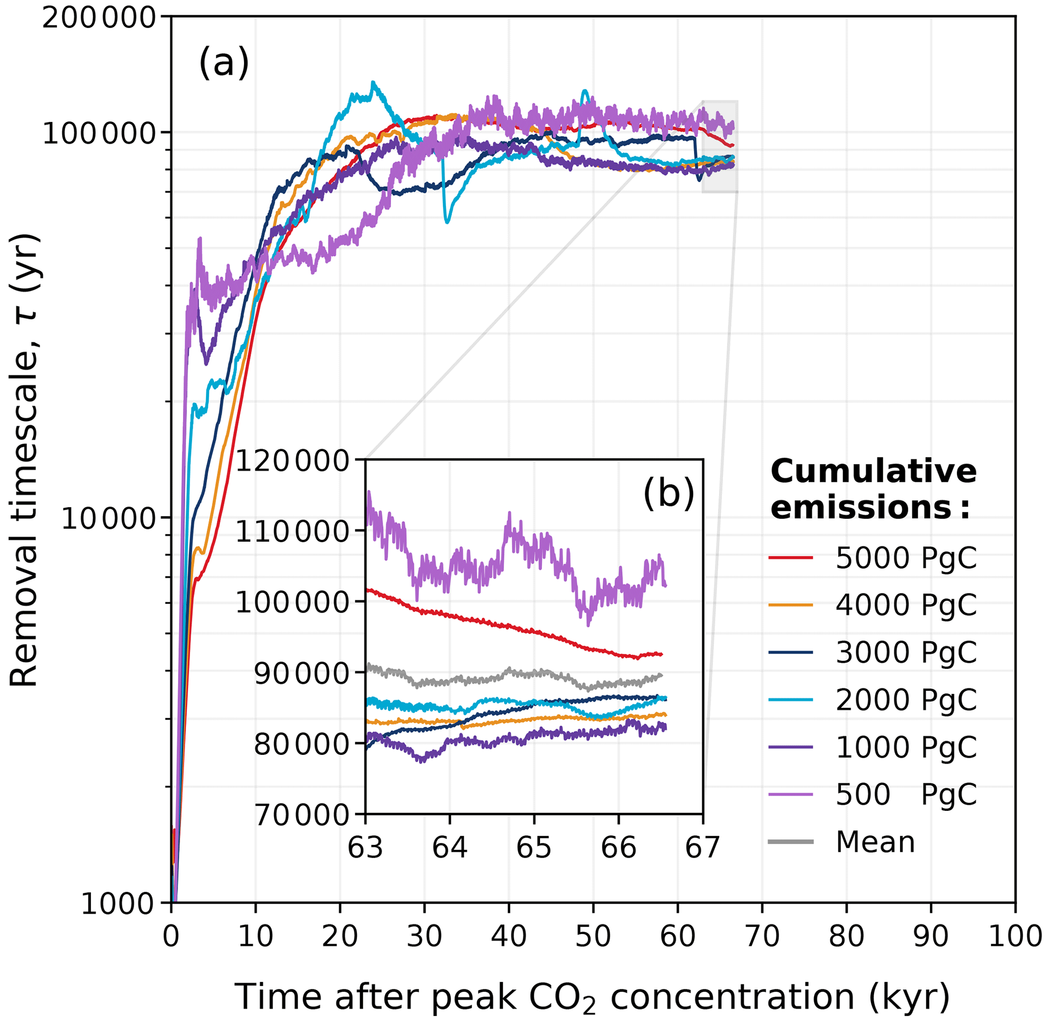
Figure 14Estimated removal timescale τ at any given time, as determined from Eq. (7) for the different emission scenarios in the REF experiment. Data have been filtered with the variable moving window discussed in Appendix D for visibility, and this is why the estimated removal timescale is not available for the full 100 kyr.
The calculated removal timescale for the REF ensemble is shown in Fig. 14a. As expected, the removal timescale is generally short in the beginning. At peak CO2 concentrations, the estimated removal timescale ranges between ∼ 0.3 and 1.6 kyr in the REF ensemble (Fig. 14a). Between 1 and 10 kyr, there is a period in time in which the removal timescale temporarily increases for the 500 and 1000 Pg C scenarios (Fig. 14a). This behaviour of the removal timescales is due to multi-millennial processes at this time, which temporarily stabilize atmospheric CO2 concentrations (since ). As this occurs around the same time as when CaCO3 reactions are particularly significant for the removal of anthropogenic CO2 (Fig. 13), it is likely related to the weak combined effect of deep-sea carbonate dissolution and terrestrial weathering in these scenarios (discussed in Sect. 3.3). At 50 kyr, the effect of carbonate weathering becomes minimal, and the removal timescale primarily reflects silicate weathering. Interestingly, the removal timescales for the ∼ 1000–4000 Pg C scenarios converge to a value lower than those in the 500 and 5000 Pg C scenarios (Fig. 14b). This generally confirms that the non-monotonic behaviour of the silicate weathering timescale seen in the multi-exponential analysis (Fig. 13) is not just an artefact of the fit. Averaging over the last 5000 years of τ(t) yields a mean removal timescale of approximately 89 kyr in the REF ensemble (range of 80–105 kyr; Fig. 14b). This method generally provides estimates of the silicate weathering timescale that are slightly lower and exhibit less spread compared to those obtained in Sect. 3.3. The multi-exponential analysis is helpful for understanding the role and removal ability of each process individually. However, this second method provides more confidence in calculating the silicate weathering timescale, as it is not influenced by factors such as the number of superimposed exponential functions (n) or the goodness of fit.
To explore the sensitivity of our results to different carbon cycle processes and climate sensitivity, we have performed a number of additional experiments (Table 1). The results from these additional experiments are discussed below. To provide a linear analysis of our sensitivity experiments, we limit our emission scenarios to ≤ 3000 Pg C. This is largely because high levels of cumulative emissions make it difficult to ignore secondary and cascading effects (e.g., shutdown of the AMOC), which would introduce nonlinearities and provide additional uncertainties.
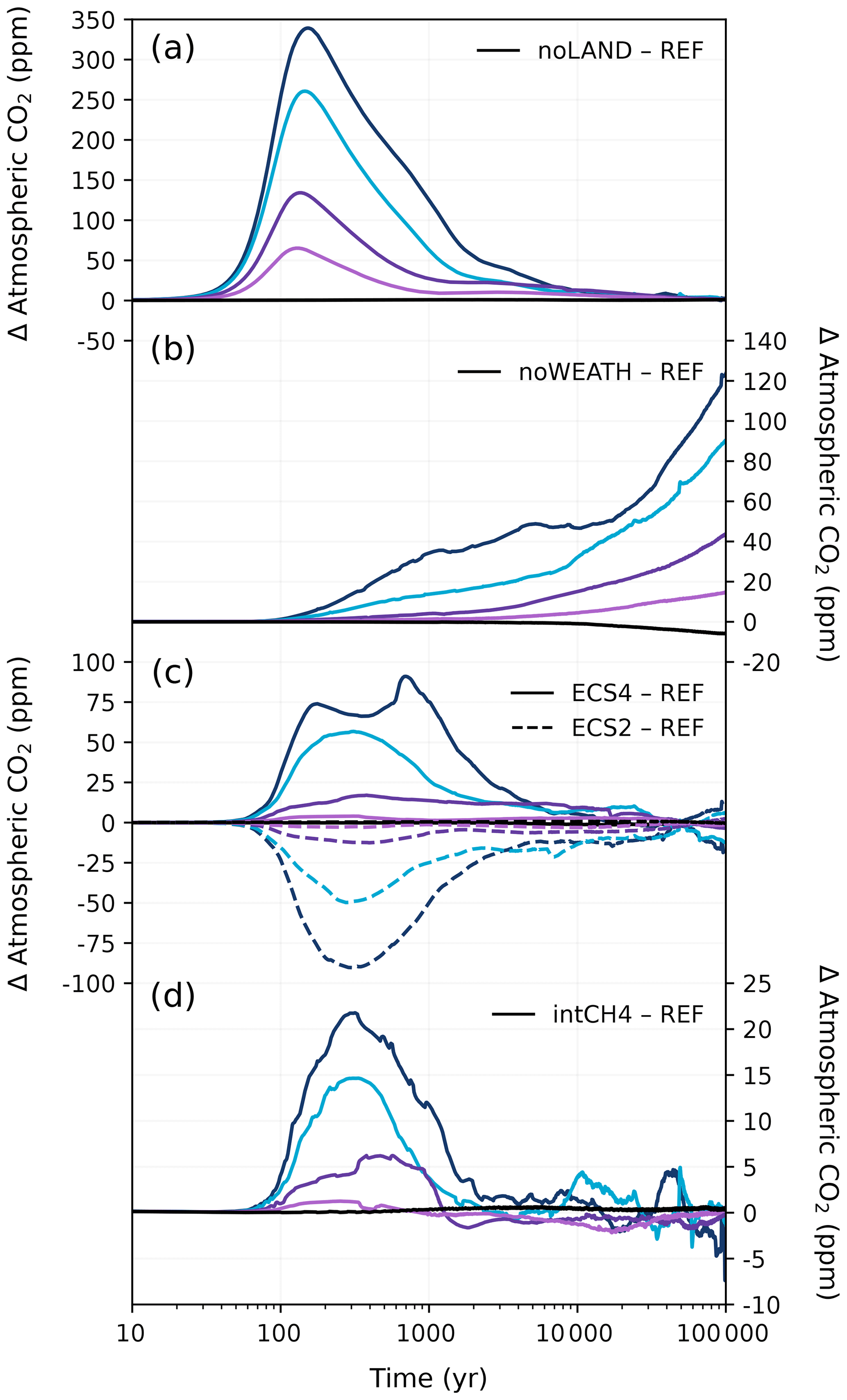
Figure 15Difference in atmospheric CO2 concentration in the different sensitivity experiments compared to the REF experiment. (a) The effect of disabling the land carbon pool. (b) The effect of constant weathering (i.e., removal of the weathering feedback). (c) The effect of a lower (2 °C) and a higher (4 °C) equilibrium climate sensitivity compared to the standard 3.1 °C in CLIMBER-X. (d) The effect of interactive methane. Negative anomaly values represent a larger atmospheric concentration in the REF experiment. Colours correspond to the cumulative emission scenarios shown in Fig. 2.
4.1 Land carbon sink
A complete disregard of the land carbon pool results in higher atmospheric CO2 concentrations at the start of our simulations (Fig. 15a). Peak atmospheric CO2 concentrations are between ∼ 65 and 340 ppm higher without the land carbon pool depending on the emission scenario. These peak magnitudes generally align with previous modelling work without a land carbon pool (Lord et al., 2015b; Köhler, 2020). After peak CO2, the difference in atmospheric CO2 concentrations between the noLAND and REF ensembles begins to decrease for all emission scenarios up to 3000 Pg C. Conversely, the carbon inventory of the ocean increases to approximately 2300 Pg C by 1 kyr, which is roughly 300 Pg C more than in the REF ensemble (Fig. 16d). The majority of this carbon uptake in the ocean occurs at peak CO2 concentration from increased air–sea CO2 flux. However, at least some of this carbon is from sediment dissolution (Fig. 16g), which contributes approximately 50 Pg C more by 1 kyr. At the beginning of the noLAND ensemble, less CO2 is absorbed on the whole, as it is taken up by relatively slow ocean and weathering processes. This leads to a higher fraction of emissions remaining in the atmosphere compared to in the REF ensemble (Fig. 17a).
It has long been recognized that land plays a crucial role in modulating the effects of weathering (Nugent and Matthews, 2012; Brault et al., 2017). However, the influence of land carbon on the long-term removal of anthropogenic CO2 through silicate weathering remains largely understudied. Since atmospheric CO2 concentrations are higher in the noLAND ensemble (Fig. 15a), peak temperatures and runoff are also elevated. As weathering in CLIMBER-X is driven by changes in runoff and temperature (see Eqs. 2 and 3), the noLAND ensemble produces higher weathering fluxes compared to the REF ensemble. This leads to a faster decline in atmospheric CO2 concentrations in the long term and a shorter silicate weathering timescale. Averaging over the last 5000 years of τ(t) in Fig. 17b yields an average value of approximately 79 kyr in the noLAND ensemble. By 100 kyr, when silicate weathering becomes the dominant carbon removal process, the higher silicate weathering in the noLAND ensemble brings atmospheric CO2 concentrations closer to those in the REF ensemble (Fig. 15a). As a result, the average fractions of emissions remaining between the REF and noLAND experiments differ by only 0.2 % at this time (Fig. 17a). The higher weathering in the noLAND ensemble therefore partially compensates for both higher initial atmospheric CO2 concentrations and a missing land carbon pool on long timescales.
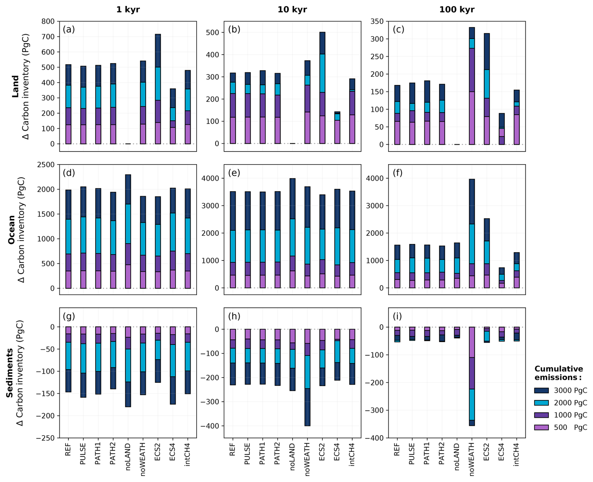
Figure 16Net cumulative uptake of carbon in the (a–c) land, (d–f) ocean, and (g–i) sediment carbon pools across the different sensitivity experiments and emission scenarios. The stacked bar plots are cumulative, meaning that the height of the bar (rather than the bar length) in each emission scenario reflects the magnitude of carbon uptake or loss. Positive values represents carbon into the land, ocean, and sediment carbon pools. The time slices of (a, d, g) 1, (b, e, h) 10, and (c, f, i) 100 kyr were chosen to capture the effects of the different timescales. It should be noted that the time slices here are measured from the start of the simulations, which includes the emissions ramp-up period.
4.2 Silicate weathering feedback
In the absence of a silicate weathering feedback, atmospheric CO2 concentrations cannot be restored back to pre-industrial conditions (Fig. 17a). Initially, atmospheric CO2 concentrations are quite similar between the REF and noWEATH ensembles, as weathering is only responsible for taking up approximately 3 % of anthropogenic CO2 within the first 1 kyr after emissions end (Fig. 3). However, the two ensembles quickly diverge as atmospheric CO2 is additionally consumed by enhanced weathering in the REF ensemble. The difference in atmospheric CO2 concentration between the REF and noWEATH grows to ∼120 ppm over the course of 100 kyr (Fig. 15). This is because the value to which atmospheric CO2 concentrations return in the noWEATH ensemble increases with larger emissions (with final values between ∼ 300 and 470 ppm compared to the pre-industrial value of 280 ppm). Across the different emission scenarios, the last ∼ 14 % (range of 13 %–15 %) of anthropogenic CO2 in the noWEATH ensemble cannot be removed without the weathering feedback (Fig. 17). This estimate is larger than what was calculated for the fraction of emissions removed by the silicate weathering timescale in the noLAND ensemble (range of 5 %–12 %; Table E2) and range provided by previous studies (range of 4 %–10 %; Lenton and Britton, 2006; Ridgwell and Hargreaves, 2007; Archer, 2005; Colbourn et al., 2015; Lord et al., 2015b; Jeltsch-Thömmes and Joos, 2020). As atmospheric CO2 concentrations do not decrease beyond ∼ 300–470 ppm in the noWEATH ensemble, temperatures stay significantly elevated (and near constant) until the end of the simulation. Climate is therefore very different in the noWEATH ensemble, resulting in notably different behaviour in the land, ocean, and sediment carbon pools compared to the REF ensemble (Fig. 16).
4.3 Climate sensitivity
The best estimate of equilibrium climate sensitivity is reported as 3 °C by the Intergovernmental Panel on Climate Change (IPCC; Canadell et al., 2021), which is close to the estimated ECS of 3.1 °C in CLIMBER-X. However, the IPCC also reports that the very likely range is 2 to 5 °C, so the effect of a lower and higher ECS (corresponding to values of 2 and 4 °C; Appendix A) was also tested. As seen in Fig. 15c, simulations using a lower ECS produce lower atmospheric concentrations of CO2 (and vice versa), and higher levels of cumulative emissions produce larger differences from the REF ensemble. The differences in atmospheric CO2 concentration can largely be traced back to changes in the land carbon inventory (Fig. 16a). In the case of ECS4, terrestrial vegetation takes up approximately the same amount of carbon as in the REF ensemble (not shown). However, increased warming causes soil carbon to become a larger source of carbon, resulting in higher atmospheric CO2 concentrations and lower land carbon across the different emission scenarios over 100 kyr. This behaviour is indicative of positive feedback as a result of warming-induced soil carbon release. For ECS2, the storage of anthropogenic CO2 in the vegetation and soil carbon pools is positive for the entire duration of the simulation regardless of the emission scenario (not shown). Despite significant variations in the partitioning of carbon between the land and ocean carbon pools (Fig. 16), differences in atmospheric CO2 concentrations between the ECS2 and ECS4 ensembles and the REF ensemble are within ∼ 5 ppm by 10 kyr and remain low for the rest of the simulation (Fig. 15c).
At first glance, this might suggest that the impact of ECS on atmospheric CO2 concentration is minimal after 10 kyr regardless of the cumulative emission scenario. Similar behaviour was also seen in Shaffer et al. (2009). However, this conclusion is only valid for a short period. In Fig. 17c, d, higher ECS values lead to a faster decline in atmospheric concentration and a shorter removal timescale of silicate weathering. Although atmospheric CO2 concentrations are initially higher in the ECS4 ensemble, they fall below those of the REF ensemble around 50 kyr due to substantial consumption by weathering (Fig. 15c). The reverse is true for ECS2. Averaging over the last 5000 years for τ(t) results in a mean silicate weathering timescale of 153 kyr for an ECS of 2 °C and 54 kyr for an ECS of 4 °C. This generally corroborates the findings by Colbourn et al. (2015), who found that a lower ECS would give a longer timescale for silicate weathering. With that in mind, the default ECS in Colbourn et al. (2015) and Lord et al. (2015b) was 2.64 °C, indicating that climate sensitivity could account for at least some of the differences in our estimated silicate weathering timescale (Fig. 13).
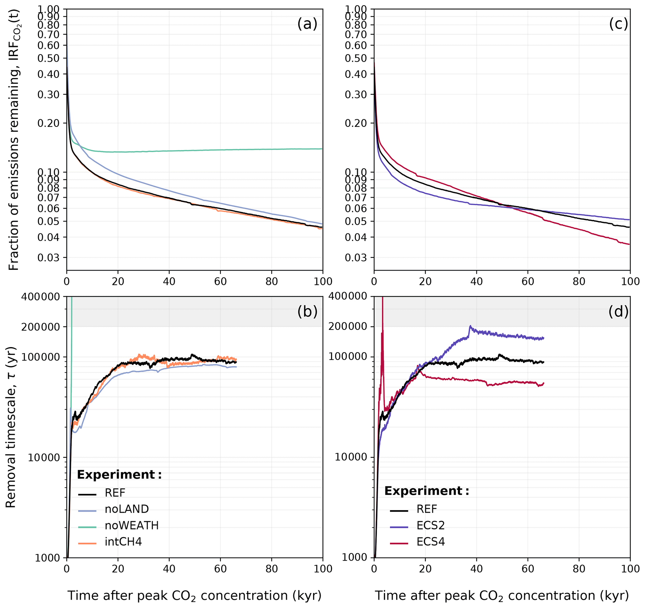
Figure 17Comparison of (a, c) the atmospheric lifetime of anthropogenic CO2 described by IRF(t) and (b, d) the removal timescale of anthropogenic CO2 in the different sensitivity experiments. The mean of the 500–3000 Pg C scenarios is shown. As described in Sects. 3.2 and 3.4, the emissions ramp-up period was excluded from the calculation of IRF(t) and τ(t). Data in (b) and (d) have been filtered with the variable moving window discussed in Appendix D for visibility, and this is why the estimated removal timescale is not available for the full 100 kyr.
4.4 Interactive methane
Global warming from anthropogenic CO2 emissions can cause additional methane emissions from natural sources that can result in an additional positive-feedback loop. Although methane has a relatively short atmospheric lifetime compared to our experiment duration (∼ 9.8 years; Voulgarakis et al., 2013), it has higher global warming potential compared to CO2. An increase in methane concentration could therefore affect the capacity of different Earth system components to take up carbon over time. For the first time, we investigate the impact of interactive methane on the long-term carbon cycle. A simple methane cycle has been implemented in CLIMBER-X that explicitly simulates the natural methane emissions from land resulting from anaerobic respiration in wetlands and peatlands (Willeit and Ganopolski, 2016). Permafrost is treated in the methane model through the representation of anaerobic decomposition in saturated soils – a process that can take place in permafrost regions. Atmospheric methane concentration is then computed with the assumption of a constant atmospheric lifetime of methane (Willeit et al., 2023).
In the zero-emissions scenario, the CH4 concentration stays largely around 600–700 ppb (close to the constant 600 ppb set in the REF ensemble; Fig. E7b). For the other scenarios (500–3000 Pg C), atmospheric CH4 concentrations rise over the first ∼ 200 years, reaching a peak of approximately 1620 ppb in the 3000 Pg C scenario. With interactive methane, atmospheric CO2 concentrations can be up to 20 ppm higher than in the REF ensemble (Fig. 15d). During much of the first 1 kyr, the differences in atmospheric CO2 concentrations between the intCH4 and REF ensembles increase with higher emissions. However, this pattern changes as atmospheric CO2 concentrations decline and does not hold beyond the first 1 kyr. The global mean temperature in the 3000 Pg C scenario is up to 0.5 °C higher in the intCH4 experiment compared to the REF experiment (Fig. E7a), but the difference remains largely negligible in the low-emission scenarios. While total vegetation carbon is similar between the REF and intCH4 ensembles, soil carbon in the intCH4 ensemble is notably lower across the different emission scenarios, causing the land carbon pool to take up less than the REF ensemble overall (Fig. 16a–c). Carbon stored in peatland is responsible for some of these differences, as carbon is lost from warming-induced soil respiration. Beyond the first 5 kyr, interactive methane has a ± 5 ppm effect on atmospheric CO2 concentration (Fig. 15d). Temperature differences between the intCH4 and REF ensembles also tend to decrease around this time, and despite small variations in how temperature evolves, the experiments largely follow each other for the rest of the simulation (Fig. E7a). In this way, the lifetime of anthropogenic CO2 and removal timescales in the intCH4 ensemble do not differ significantly from those in the REF ensemble over long timescales (Fig. 17a, b), suggesting that the indirect effect of CH4 on the climate (through CO2) is likely negligible over such periods.
The impacts of anthropogenic climate change will likely be felt for tens of thousands if not hundreds of thousands of years – long after the anthropogenic emission of CO2 has ended. By simulating the long-term response to idealized emission scenarios, we highlighted how processes that remove carbon from the atmosphere change with different levels of cumulative emissions. With this, we have examined the capacity of these processes and extent to which they take up carbon on different timescales. To some extent, the results of this study align with previous investigations. For example, we have shown that the magnitude of cumulative emissions will predominantly control the long-term response, supporting the path independence found by previous work (Matthews et al., 2009; Zickfeld et al., 2012; Herrington and Zickfeld, 2014). The decline in anthropogenic CO2 over time seen here generally falls within estimates given by the multi-model assessment in Archer et al. (2009a) and other studies: approximately 10 % of anthropogenic emissions will persist longer than 10 000 years and ∼ 4 % beyond 100 000 years. The response of deep-ocean processes and CaCO3 reactions, as well as their ability to remove anthropogenic CO2 at different levels of cumulative emissions, also supports earlier investigations (Lord et al., 2015b). However, the extensive sensitivity analysis, along with the higher resolution and complexity of CLIMBER-X, have lead to several new findings.
-
The removal timescale of silicate weathering is significantly influenced by a number of factors. In this study, we quantified the effects of climate sensitivity, the land carbon pool, weathering feedbacks, and dynamically changing methane concentrations on the atmospheric lifetime of anthropogenic CO2. The sensitivity analysis revealed that climate sensitivity has the most significant influence on the silicate weathering timescale (Fig. 17). However, most factors were generally found to impact the silicate weathering timescale, albeit in opposing ways. Our results show that higher climate sensitivity, stronger silicate weathering feedbacks, a spatially explicit weathering scheme, and no land carbon pool reduce the removal timescale of silicate weathering, whereas lower climate sensitivity and a land carbon pool increase this timescale. This means that in theory, the same silicate weathering timescale could be obtained with no land carbon and either weaker weathering feedbacks or lower ECS. This emphasizes the importance of incorporating as many components of the carbon cycle as possible and increasing model complexity in Earth system models to more accurately represent the long-term future behaviour of atmospheric CO2. Furthermore, the global heterogeneity of carbonate and silicate weathering with increasing emissions (Fig. 11) also showed the importance of highly active weathering regions for the global weathering flux (Sect. 3.1.3), highlighting the need for spatially explicit schemes. Improving the silicate weathering timescale would require more accurate constraints on both these factors and the global silicate weathering flux and would require a deeper understanding of how weathering responds to increasing global temperatures.
-
The removal timescale of silicate weathering is significantly shorter than previously estimated. The two methods used in this study provided significantly shorter removal timescales for silicate weathering compared to previous research, providing a best estimate of 80–105 kyr depending on the emission size. This discrepancy is likely due to differences in climate sensitivity, weathering feedbacks, the spatially explicit weathering scheme, and the land carbon pool. With this in mind, our estimates here do not address (potentially large) uncertainties related to the sensitivity of silicate weathering processes, such as erosion limitation or net primary production on land. Nevertheless, it is worth noting that ∼ 20–30 years has passed since the constant 200–400 kyr range was first established for the silicate weathering timescale using lower-complexity models (Sundquist, 1991; Archer et al., 1997, 1998), and our results indicate that it is time to re-examine this estimate. Considering the large uncertainty that exists in the literature concerning its value and the progress made in model resolution and process descriptions in our model and others since the last LTMIP, another intercomparison project could be beneficial.
-
The removal timescale of silicate weathering is dependent on the magnitude of cumulative emissions. A major finding in Lord et al. (2015b) was that the removal ability and timescale of silicate weathering were approximately invariant with respect to cumulative emissions. This is challenged here, as it was shown that both are non-monotonic with increasing emissions. In all experiments that were analyzed (REF, PULSE, and noLAND), there is an initial shortening of the silicate weathering timescale with increasing cumulative emissions until ∼ 3000–4000 Pg C. For the 5000 Pg C scenario, however, it was found (via two methods) that the timescale increases. Whether this trend persists for emissions beyond 5000 Pg C remains to be determined. Future research would benefit from exploring the connection between the extended AMOC decline and the long-term removal of anthropogenic CO2 via silicate weathering.
-
Land carbon has a significant long-term influence on the future evolution of atmospheric CO2. Despite variations in vegetation and soil carbon response with increasing emissions, the terrestrial storage of anthropogenic carbon is positive for the duration of our simulations and is responsible for storing approximately 4 %–13 % of anthropogenic carbon by the end of the simulation. The land's capacity to absorb anthropogenic CO2 in the simulations buffers higher CO2 concentrations and, therefore, peak global temperatures. As a consequence, the inclusion of land carbon cycle processes effectively reduces weathering fluxes, thereby increasing the removal timescale of silicate weathering. Experiments that exclude land carbon would show a shorter silicate weathering timescale than those that include land carbon. As silicate weathering is the ultimate control of the removal of anthropogenic CO2, the extent to which the land buffers peak temperature in a model can significantly influence the atmospheric lifetime of anthropogenic CO2.
-
The methane cycle will likely have a negligible effect on long timescales (> 103 years). Rising global temperatures will increase methane levels, potentially amplifying positive feedbacks and impacting how Earth system components absorb carbon over time. These experiments show that a dynamic methane cycle in CLIMBER-X can contribute up to an additional ∼ 25 ppm in atmospheric CO2 concentration. However, this effect is mainly limited to the first millennium after emissions end and is largely negligible on long timescales. As such, the methane cycle does not contribute to substantially different removal timescales, leading to the same rate of anthropogenic CO2 removal over time as in the REF ensemble.
There are several assumptions in our study that should be considered when generalizing the long-term response of the climate–carbon system. Certain aspects of the carbon cycle in CLIMBER-X are simplified or not considered, as current computational restrictions limit the inclusion of all carbon cycle processes across all timescales. For example, CLIMBER-X does not consider deep-sea methane hydrates or nitrogen limitation in tropical or boreal forests, despite their potential impacts on future carbon uptake (Archer et al., 2009b; Norby et al., 2010). Some general uncertainties and poor empirical constraints should also be considered, as they can inhibit an accurate description of some processes. One such example is the strength of the biological pump in a warming world. Although state-of-the-art Earth system models do not agree on the overall response of marine primary production to increasing CO2 levels on centennial timescales (Laufkötter et al., 2015), widespread ocean acidification is still expected to have some influence (Mora et al., 2013). This is not considered in our model, which relies on an extended NPZD (nutrients–phytoplankton–zooplankton–detritus) description, typical of models at this level of complexity. The weathering scheme used in CLIMBER-X is significantly more advanced than in other models of the same class; however, it does not explicitly account for changes in vegetation cover or net primary production. While this could be an important simplification, it is presently unclear to what extent it may affect long-term CO2 dynamics. As 10 % of the land area in our simulations is responsible for more than a third of global silicate weathering fluxes, small changes in the controlling parameters in these areas can also significantly impact total weathering fluxes (Hartmann et al., 2009b). Like many other models, CLIMBER-X also does not account for the potentially significant effect of soil shielding, given the limited quantity of data and the ongoing uncertainties regarding their impact. However, there is some evidence to suggest that erosion limitation could weaken the strength of the weathering feedback (Goddéris et al., 2008; Maher and Chamberlain, 2014; Maffre et al., 2023), which may increase the estimated removal timescale of silicate weathering. These limitations highlight potential directions for further work.
A few studies (Lenton and Britton, 2006; Lord et al., 2015b; Köhler, 2020; Couplet et al., 2025) have looked at idealized emission scenarios with more than ∼6000 Pg C, corresponding to unconventional fossil fuels. This was not considered here, partially because the potential of unconventional fossil fuels is still speculative but also because such high levels of cumulative emissions make it difficult to ignore additional changes in the Earth system, such as sea level rise. Simulations in this study were carried out using prescribed present-day ice sheets to maintain consistency with previous research. However, the melting of the Greenland and West Antarctic ice sheets, inevitable in high-emission scenarios, can introduce additional feedback mechanisms into the carbon cycle (Wadham et al., 2019). These effects could be significant for the range of emissions considered here. Moreover, significant global warming is expected to trigger the crossing of one (or more) critical thresholds in the Earth system (Lenton et al., 2008; Armstrong McKay et al., 2022; Wunderling et al., 2024), which could affect the long-term capacity of different components to absorb carbon over time. In addition to this, it has been assumed that the pre-industrial global carbon cycle was in equilibrium, such that the silicate weathering feedback will eventually return the CO2 concentrations to 280 ppm after an anthropogenic perturbation in the carbon cycle. This assumption can also be explicitly seen in the zero-emissions scenario in Fig. 2. While this is a standard assumption for investigations into the long-term response of the climate-carbon system to perturbations in the carbon cycle, it is perhaps not so appropriate for the very long timescales considered in this work. The implications of this assumption will be considered in a forthcoming paper. Future work with the CLIMBER-X model will investigate the long-term effects of anthropogenic CO2 on the dynamic evolution of Northern Hemisphere ice sheets.
Previous studies have implemented straightforward ways to scale ECS (e.g., Colbourn et al., 2015). In CLIMBER-X, different climate sensitivities can be achieved by scaling the equivalent CO2 in the long-wave radiation scheme in the following way:
where α is the scaling coefficient and CO ppm. The equivalent CO2 concentration for radiation is CO, which also includes the effect of other greenhouse gases (Willeit et al., 2023). It was determined a priori that α=0.66 yielded an ECS of 2 °C, whereas α=1.33 yielded an ECS of 4 °C. This method has been more extensively applied in Höning et al. (2024) and Kaufhold et al. (2025b). More information about this ECS scaling technique in CLIMBER-X, as well as a comparison with state-of-the-art Earth system models, can be found in Kaufhold et al. (2025b).
The fraction of the different carbon reservoirs that contribute to the removal of anthropogenic CO2 over a span of 100 kyr is assessed using Eq. (B3). This is similar to calculations for airborne, land-borne, ocean-borne, and sediment-borne fractions (Jones et al., 2013; Vakilifard et al., 2022), as the cumulative carbon fluxes of the atmosphere, land, ocean, and weathering are normalized by cumulative anthropogenic emissions, E (Pg C). However, we focus strictly on changes in cumulative carbon flux from the atmosphere relative to the pre-industrial state instead of changes in the carbon inventory, as our experiments were conducted with an open carbon cycle. From Eq. (1), we get
which, integrated in time, gives
As we only consider times after the cessation of anthropogenic emissions (i.e., , total cumulative emissions), the equation above becomes
The individual components seen in Fig. 3 are then computed as follows:
Fluxes (in Pg C yr−1) are relative to the average flux over the reference simulation to account for model drift. We add and subtract from Focn and Fweath, respectively, as carbonate weathering additionally transfers carbon into the ocean and causes ocean outgassing. Volcanic outgassing, Fvolc, was additionally subtracted from Fweath to isolate silicate weathering consumption.
The Revelle factor ξ quantifies the ocean's ability to absorb CO2. It essentially compares the ratio of fractional changes in CO2 to the fractional changes in DIC (Sarmiento and Gruber, 2006), making it a useful metric to assess the sensitivity of our simulations to anthropogenic CO2 perturbations (Broecker et al., 1979). Given that there are competing definitions in the literature (see: Egleston et al., 2010), we explicitly calculate the Revelle factor in the following way:
One disadvantage of the formulation for τ(t) in Sect. 3.4 is that it is sensitive to small-scale variability and noise in CO2(t). A simple rolling mean is not sufficient to smooth this, as the removal timescale is expected to increase over time, eventually converging to an 𝒪(105−6) timescale that is representative of silicate weathering. For this reason, we use a forward-rolling mean to remove noise on both short and long timescales. While a rolling mean is generally defined with a fixed window size, we modified the standard equation to have a variable window size. This can be written as follows:
where w(t) is the window size as a function of time, t is time, CO2(t) is the atmospheric CO2 concentration at time t, and CO is the peak CO2 concentration. Different functions were tested for w(t), but following a simple, linearly increasing window of provided the best results, as it still preserved the overall trend on multiple timescales. Given data limitations, the rolling window could not extend beyond 100 kyr due to the forward-rolling technique. For this reason, the data are cut around approximately t≈ 67 kyr, when the window size becomes approximately w(t)≈ 33 kyr, and this is why data for the full 100 kyr are not shown in Figs. 14 and 17b, d.
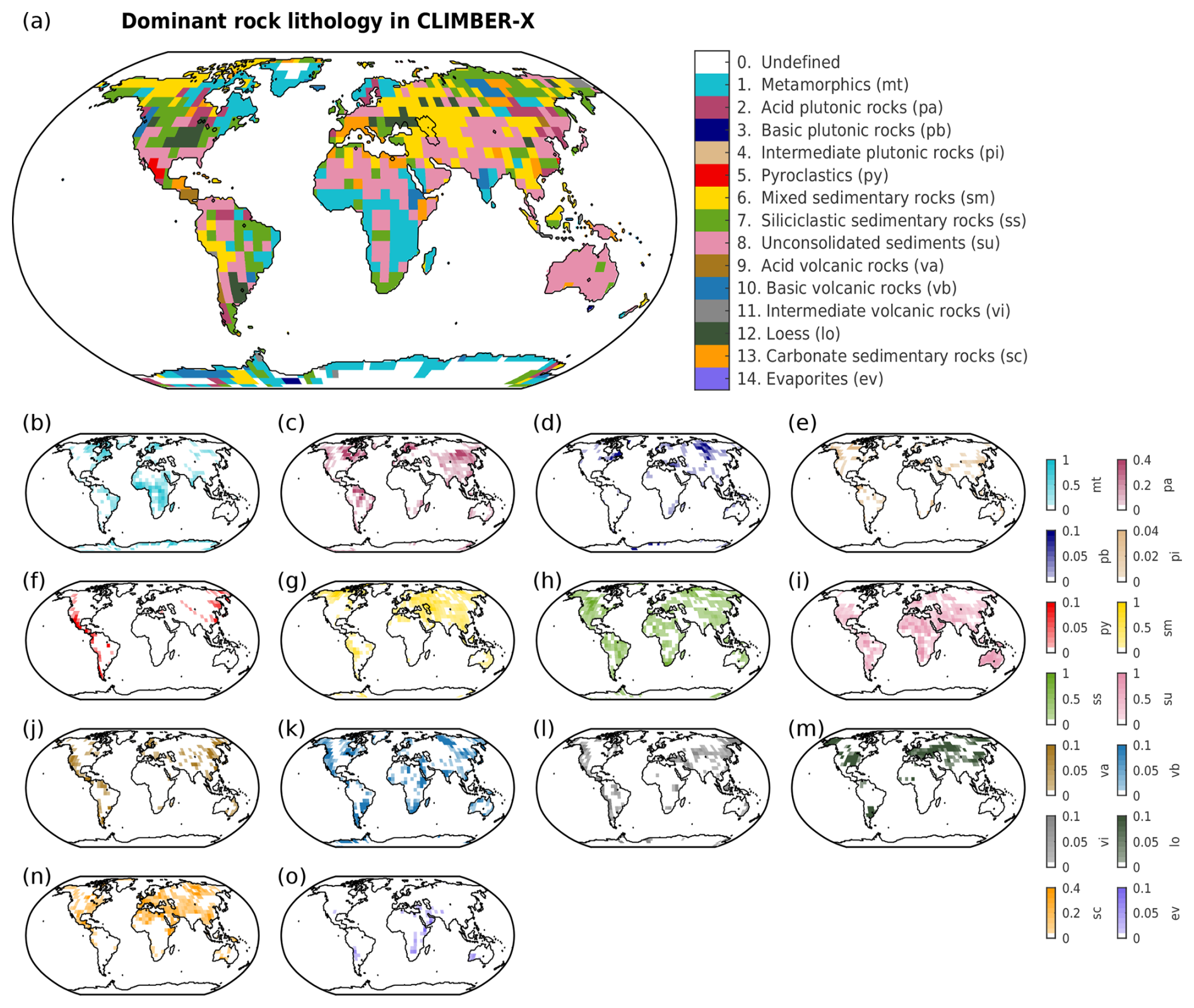
Figure E1Distribution of the 14 lithological classes implemented in CLIMBER-X for the present day. These are based on the GLiM lithological map (Hartmann and Moosdorf, 2012). The dominant rock type in a given grid cell is shown in (a). The spatial distribution of grid cell lithological fractions, β(ℓ), is given for (b) metamorphic rocks, (c) acid plutonic rocks, (d) basic plutonic rocks, (e) intermediate plutonic rocks, (f) pyroclastics, (g) mixed sedimentary rocks, (h) siliciclastic sedimentary rocks, (i) unconsolidated sediments, (j) acid volcanic rocks, (k) basic volcanic rocks, (l) intermediate volcanic rocks, (m) loess, (n) carbonate sedimentary rocks, and (o) evaporites. Note that the colour bar range for different lithological fractions changes between lithological classes.
Table E1Lithological classes in CLIMBER-X. These are based on the lithological map of GLiM (Hartmann and Moosdorf, 2012), and the activation energy of silicates is from Hartmann et al. (2014). The evaporites class (ev) is used only to compute phosphorus fluxes in CLIMBER-X and is therefore also not considered here.
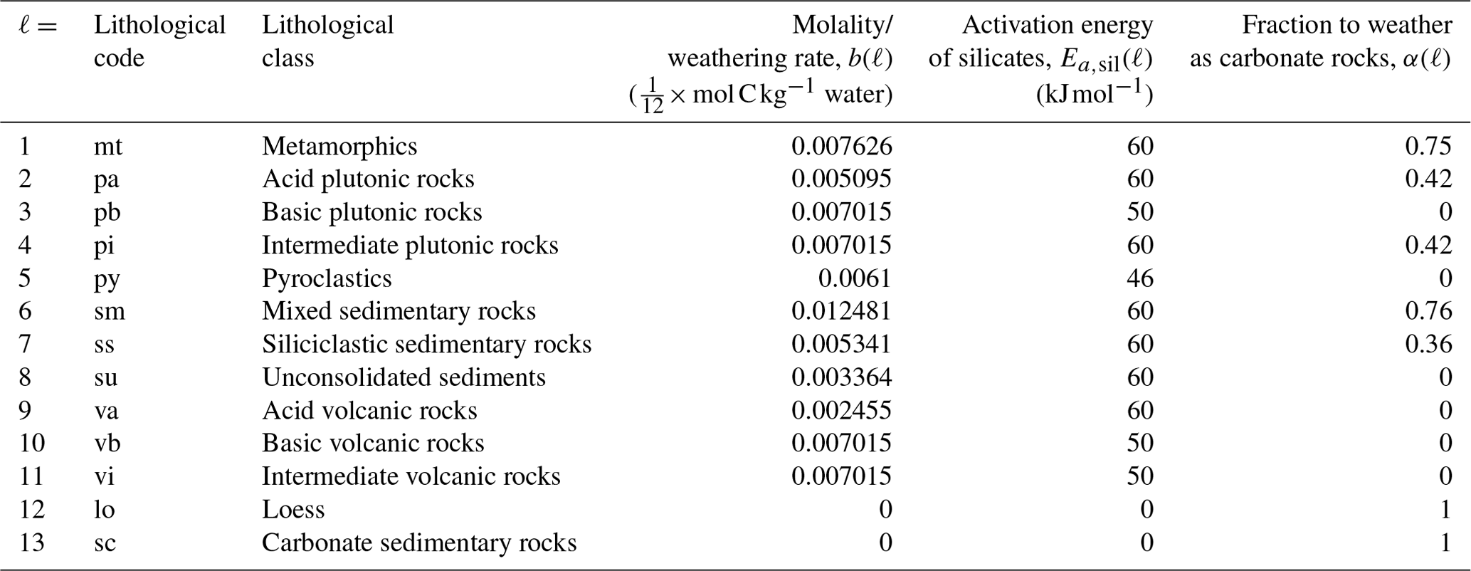
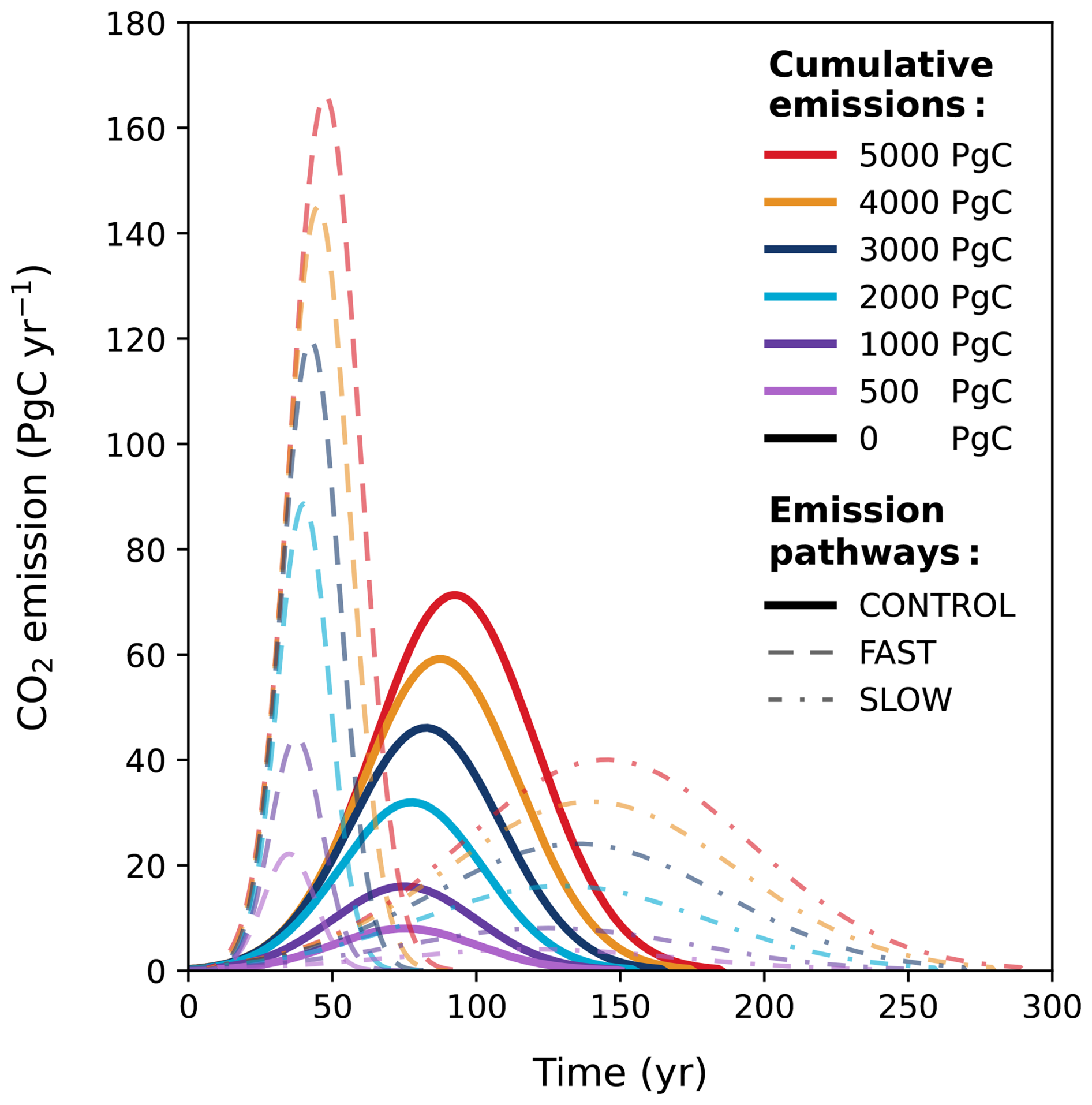
Figure E2Pathways of emitted carbon as described by three different functions. A fourth pathway called “pulse”, not shown here, assumes that all anthropogenic emissions are released in the first time step of the simulation.
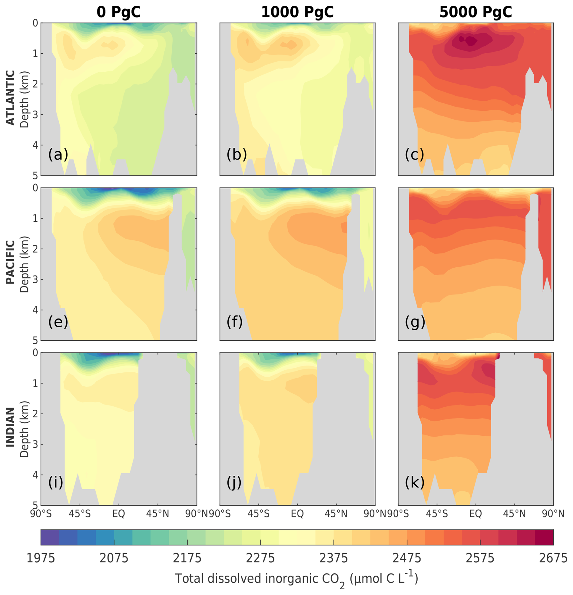
Figure E3Annual mean dissolved inorganic CO2 in three oceanic basins at 1 kyr. The top row (a)–(c) shows the zonal mean cross section of the Atlantic Ocean, the middle row (d)–(f) shows the Pacific Ocean, and the bottom row (g)–(i) shows the Indian Ocean. The time slice here is measured from the start of the simulations, meaning that it includes the emissions ramp-up period.
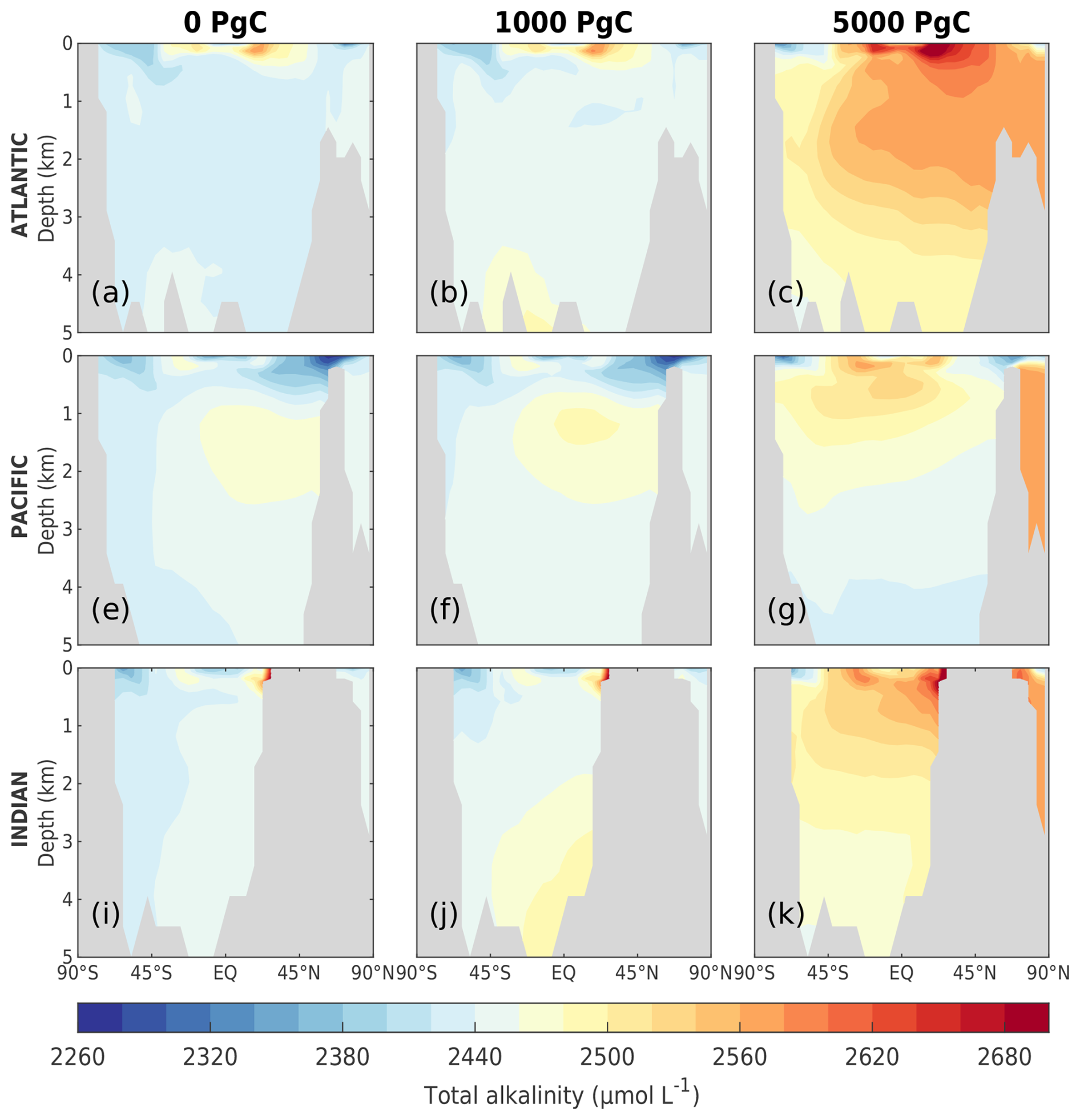
Figure E4Annual mean alkalinity in three oceanic basins at 1 kyr. The top row (a–c) shows the zonal mean cross section of the Atlantic Ocean, the middle row (d–f) shows the Pacific Ocean, and the bottom row (g–i) shows the Indian Ocean. The time slice here is measured from the start of the simulations, meaning that it includes the emissions ramp-up period.
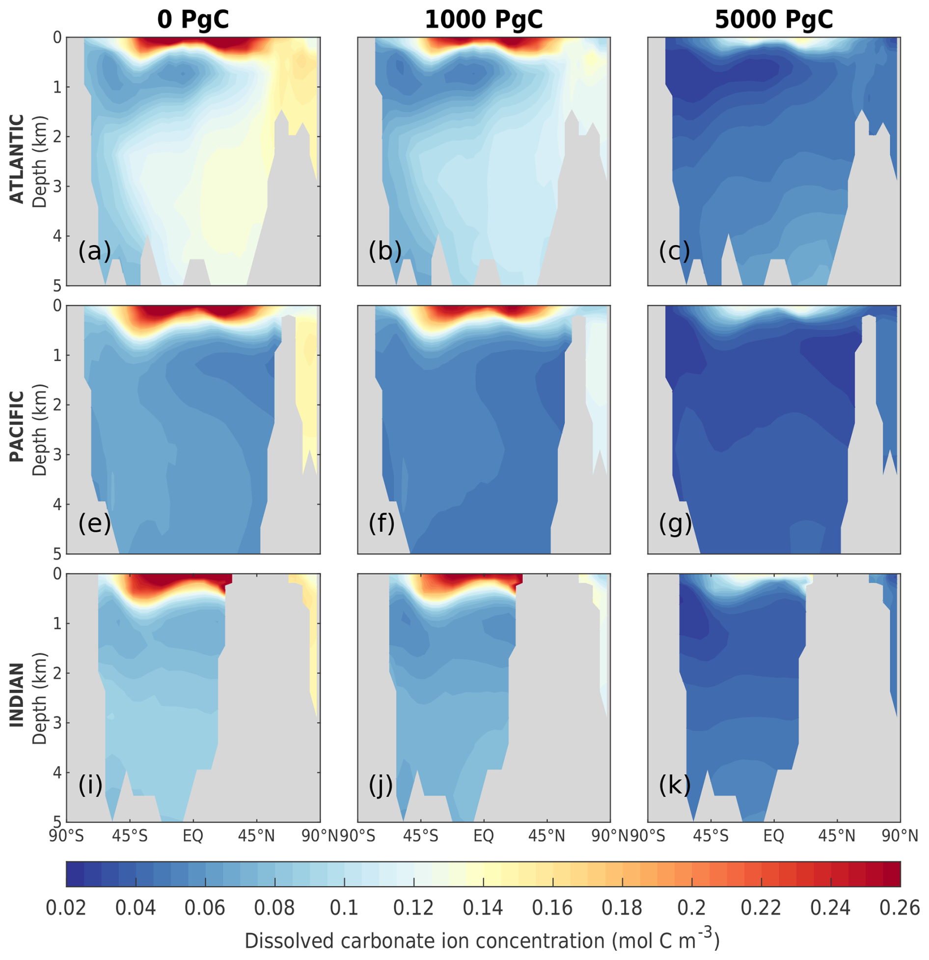
Figure E5Annual mean dissolved carbonate ion concentration in three oceanic basins at 1 kyr. The top row (a–c) shows the zonal mean cross section of the Atlantic Ocean, the middle row (d–f) shows the Pacific Ocean, and the bottom row (g–i) shows the Indian Ocean. The time slice here is measured from the start of the simulations, meaning that it includes the emissions ramp-up period.
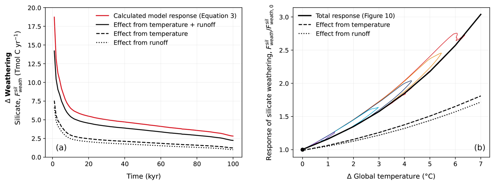
Figure E6Contribution of temperature and runoff to the silicate weathering response in CLIMBER-X. (a) Change in silicate weathering flux from the pre-industrial value (12.3 Tmol C yr−1) for the 5000 Pg C scenario. The contributions from temperature and runoff were broken down for the 5000 Pg C scenario, and they do not linearly add to the calculated model response, as the weathering relation in Eq. (3) is nonlinear. (b) Response in silicate weathering as a function of global mean temperature. Like Fig. 10, the fit of these trajectories has been plotted above using Numpy.Polyfit in Python. The relative contributions of temperature and runoff to the silicate weathering response were determined from the 5000 Pg C scenario, i.e., the trajectories from (a).
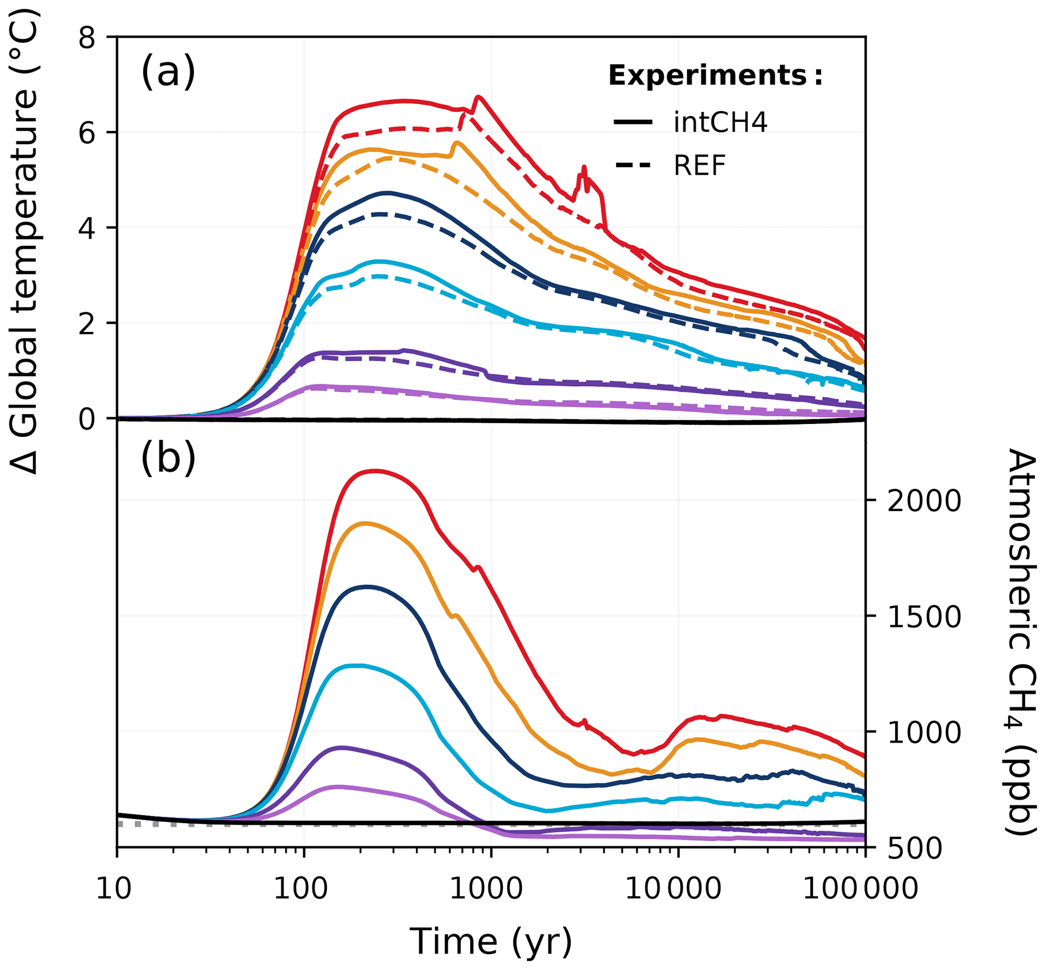
Figure E7Changes in (a) global temperature and (b) atmospheric CH4 concentration in the intCH4 experiment compared to the REF experiment. The dotted grey line here in (b) shows the constant CH4 concentration used in the REF experiment (600 ppb). Colours correspond to the cumulative emission scenarios shown in Fig. 2.
Table E2Fitting parameters used for a multi-exponential decay function describing atmospheric CO2 concentration in the REF, PULSE, and noLAND experiments. Here, the fraction of emissions (Ai) taken up over the removal timescales (τi) associated with ocean invasion (i=1), CaCO3 reactions (i=2), and silicate weathering (i=3) are shown. We highlight the fact that this is the total fraction of emissions removed after peak CO2 concentrations have been reached. Anthropogenic CO2 removed during the ramp-up of emissions is not considered in this analysis. The fraction of emissions removed from short-term (sub-centennial timescales) processes can be broadly estimated from . While n=3 was used for consistency across experiments, we acknowledge that a more accurate fit for the PULSE ensemble could theoretically be achieved by increasing the number of fitted exponentials (as in Colbourn et al., 2015; Lord et al., 2015b).
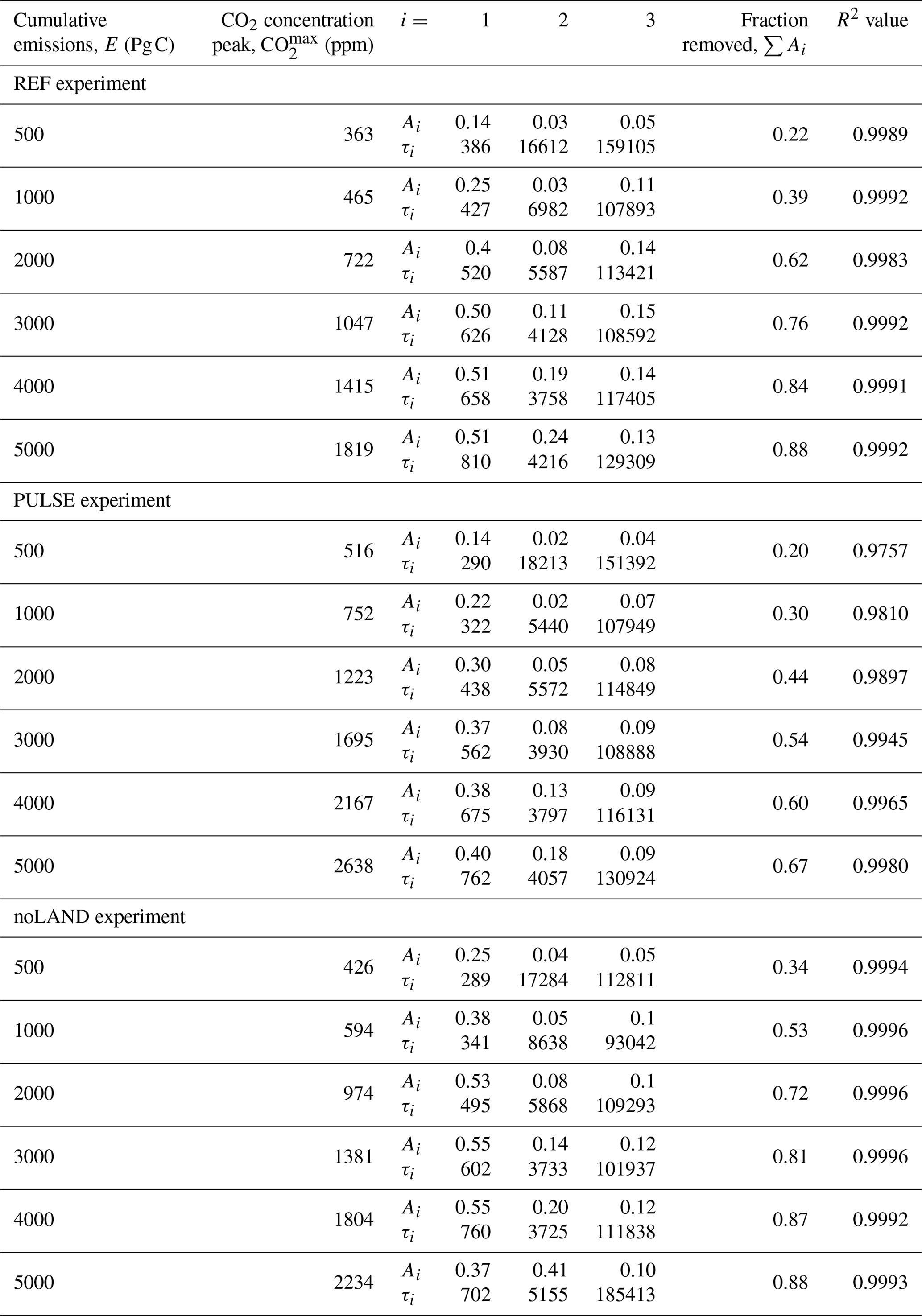
The code and model output can be obtained from https://doi.org/10.5281/zenodo.13933974 (Kaufhold et al., 2025a).
Experimental setup and design was led by MW and AG. CK conducted the simulations and wrote the paper with support from MW, BL, and AG. All authors contributed to the analysis, discussion, and general quality of the text.
The contact author has declared that none of the authors has any competing interests.
Publisher’s note: Copernicus Publications remains neutral with regard to jurisdictional claims made in the text, published maps, institutional affiliations, or any other geographical representation in this paper. While Copernicus Publications makes every effort to include appropriate place names, the final responsibility lies with the authors.
Christine Kaufhold is funded by the Bundesgesellschaft für Endlagerung through the URS project (research project no. STAFuE-21-4-Klei). Matteo Willeit is supported by the German paleoclimate modelling initiative PalMod (grant nos. 01LP1920B, 01LP1917D, 01LP2305B). Bo Liu is supported by the German paleoclimate modelling initiative PalMod (grant nos: 01LP1919B, 01LP2328A). PalMod is part of the Research for Sustainable Development initiative (FONA) funded by the German Federal Ministry of Education and Research (BMBF). The authors gratefully acknowledge the European Regional Development Fund (ERDF), the German Federal Ministry of Education and Research, and the state of Brandenburg for supporting this project by providing resources on the high-performance computer system at the Potsdam Institute for Climate Impact Research. We additionally thank Victor Couplet for helpful discussions and SURFER model output, as well as Richard Zeebe and Peter Köhler for their valuable feedback and suggestions during the peer-review process.
This research has been supported by the Bundesgesellschaft für Endlagerung (research project no. STAFuE-21-4-Klei) and the German Federal Ministry of Education and Research (BMBF) (grant nos. 01LP1920B, 01LP1917D, 01LP2305B, 01LP1919B, and 01LP2328A).
The article processing charges for this open-access publication were covered by the Potsdam Institute for Climate Impact Research (PIK).
This paper was edited by Olivier Sulpis and reviewed by Amber Boot, Pierre Maffre, and one anonymous referee.
Amiotte Suchet, P. and Probst, J.-L.: A global model for present-day atmospheric/soil CO2 consumption by chemical erosion of Continental Rocks (Gem-CO2), Tellus B, 47, 273–280, https://doi.org/10.1034/j.1600-0889.47.issue1.23.x, 1995. a
Amiotte Suchet, P., Probst, J.-L., and Ludwig, W.: Worldwide distribution of continental rock lithology: Implications for the atmospheric/soil CO2 uptake by continental weathering and alkalinity river transport to the oceans, Global Biogeochem. Cy., 17, 1038, https://doi.org/10.1029/2002GB001891, 2003. a, b
Archer, D.: Fate of fossil fuel CO2 in geologic time, J. Geophys. Res., 110, C09S05, https://doi.org/10.1029/2004jc002625, 2005. a, b, c, d, e, f, g
Archer, D. and Brovkin, V.: The millennial atmospheric lifetime of anthropogenic CO2, Climatic Change, 90, 283–297, https://doi.org/10.1007/s10584-008-9413-1, 2008. a, b, c, d, e
Archer, D. and Ganopolski, A.: A movable trigger: Fossil fuel CO2 and the onset of the next glaciation, Geochem. Geophy. Geosy., 6, Q05003, https://doi.org/10.1029/2004GC000891, 2005. a
Archer, D., Kheshgi, H., and Maier-Reimer, E.: Multiple timescales for neutralization of fossil fuel CO2, Geophys. Res. Lett., 24, 405–408, https://doi.org/10.1029/97gl00168, 1997. a, b, c, d, e, f, g, h, i, j, k
Archer, D., Kheshgi, H., and Maier-Reimer, E.: Dynamics of fossil fuel CO2 neutralization by marine CaCO3, Global Biogeochem. Cy., 12, 259–276, https://doi.org/10.1029/98GB00744, 1998. a, b, c
Archer, D., Eby, M., Brovkin, V., Ridgwell, A., Cao, L., Mikolajewicz, U., Caldeira, K., Matsumoto, K., Munhoven, G., Montenegro, A., and Tokos, K.: Atmospheric lifetime of fossil fuel carbon dioxide, Annu. Rev. Earth Pl. Sc., 37, 117–134, https://doi.org/10.1146/annurev.earth.031208.100206, 2009a. a, b, c, d, e, f, g, h, i, j
Archer, D., Buffett, B., and Brovkin, V.: Ocean methane hydrates as a slow tipping point in the global carbon cycle, P. Natl. Acad. Sci. USA, 106, 20596–20601, https://doi.org/10.1073/pnas.0800885105, 2009b. a
Armstrong McKay, D. I., Staal, A., Abrams, J. F., Winkelmann, R., Sakschewski, B., Loriani, S., Fetzer, I., Cornell, S. E., Rockström, J., and Lenton, T. M.: Exceeding 1.5 °C global warming could trigger multiple climate tipping points, Science, 377, eabn7950, https://doi.org/10.1126/science.abn7950, 2022. a
Beck, J., Bock, M., Schmitt, J., Seth, B., Blunier, T., and Fischer, H.: Bipolar carbon and hydrogen isotope constraints on the Holocene methane budget, Biogeosciences, 15, 7155–7175, https://doi.org/10.5194/bg-15-7155-2018, 2018. a
Berger, A. and Loutre, M. F.: An exceptionally long interglacial ahead?, Science, 297, 1287–1288, https://doi.org/10.1126/science.1076120, 2002. a
Bluth, G. and Kump, L.: Phanerozoic paleogeology, Am. J. Sci., 291, 284–308, https://doi.org/10.2475/ajs.291.3.284, 1991. a
Brault, M.-O., Matthews, H. D., and Mysak, L. A.: The importance of terrestrial weathering changes in multimillennial recovery of the global carbon cycle: a two-dimensional perspective, Earth Syst. Dynam., 8, 455–475, https://doi.org/10.5194/esd-8-455-2017, 2017. a, b, c
Broecker, W. S., Takahashi, T., Simpson, H. J., and Peng, T. H.: Fate of Fossil Fuel Carbon Dioxide and the Global Carbon Budget, Science, 206, 409–418, https://doi.org/10.1126/science.206.4417.409, 1979. a
Brovkin, V., Boysen, L., Arora, V. K., Boisier, J. P., Cadule, P., Chini, L., Claussen, M., Friedlingstein, P., Gayler, V., van den Hurk, B. J., and Hurtt, G. C. and Jones, C. D. and Kato, E. and de Noblet-Ducoudré, N. and Pacifico, F. and Pongratz, J., and Weiss, M.: Effect of anthropogenic land-use and land-cover changes on climate and land carbon storage in CMIP5 projections for the twenty-first century, J. Clim., 26, 6859–6881, https://doi.org/10.1175/jcli-d-12-00623.1, 2013. a
Börker, J., Hartmann, J., Amann, T., Romero-Mujalli, G., Moosdorf, N., and Jenkins, C.: Chemical weathering of loess and its contribution to global alkalinity fluxes to the coastal zone during the Last Glacial Maximum, mid-Holocene, and present, Geochem. Geophy. Geosy., 21, e2020GC008922, https://doi.org/10.1029/2020GC008922, e2020GC008922 2020GC008922, 2020. a, b
Caldeira, K. and Wickett, M. E.: Ocean model predictions of chemistry changes from carbon dioxide emissions to the atmosphere and ocean, J. Geophys. Res.-Ocean., 110, C09S04, https://doi.org/10.1029/2004JC002671, 2005. a
Canadell, J., Monteiro, P., Costa, M., Cotrim da Cunha, L., Cox, P., Eliseev, A., Henson, S., Ishii, M., Jaccard, S., Koven, C., Lohila, A., Patra, P., Piao, S., Rogelj, J., Syampungani, S., Zaehle, S., and Zickfeld, K.: Chap. 5: Global carbon and other biogeochemical cycles and feedbacks, in: Climate Change 2021: The Physical Science Basis, Contribution of Working Group I to the Sixth Assessment Report of the Intergovernmental Panel on Climate Change, edited by: Masson-Delmotte, V., Zhai, P., Pirani, A., Connors, S., Péan, C., Berger, S., Caud, N., Chen, Y., Goldfarb, L., Gomis, M., Huang, M., Leitzell, K., Lonnoy, E., Matthews, J., Maycock, T., Waterfield, T., Yelekçi, O., Yu, R., and Zhou, B., 673–816, Cambridge University Press, Cambridge, United Kingdom and New York, NY, USA, https://doi.org/10.1017/9781009157896.007, 2021. a
Cawley, G. C.: On the atmospheric residence time of anthropogenically sourced carbon dioxide, Energ. Fuel., 25, 5503–5513, https://doi.org/10.1021/ef200914u, 2011. a
Charbit, S., Paillard, D., and Ramstein, G.: Amount of CO2 emissions irreversibly leading to the total melting of Greenland, Geophys. Res. Lett., 35, L12503, https://doi.org/10.1029/2008gl033472, 2008. a, b
Colbourn, G.: Weathering effects on the carbon cycle in an Earth System Model, PhD Thesis, University of East Anglia, Norwich, UK, https://ueaeprints.uea.ac.uk/id/eprint/34242/ (last access: 18 September 2024), 2011. a
Colbourn, G., Ridgwell, A., and Lenton, T. M.: The Rock Geochemical Model (RokGeM) v0.9, Geosci. Model Dev., 6, 1543–1573, https://doi.org/10.5194/gmd-6-1543-2013, 2013. a, b, c
Colbourn, G., Ridgwell, A., and Lenton, T. M.: The time scale of the silicate weathering negative feedback on atmospheric CO2, Global Biogeochem. Cy., 29, 583–596, https://doi.org/10.1002/2014GB005054, 2015. a, b, c, d, e, f, g, h, i, j, k, l, m, n, o, p, q, r
Couplet, V., Martínez Montero, M., and Crucifix, M.: SURFER v3.0: a fast model with ice sheet tipping points and carbon cycle feedbacks for short- and long-term climate scenarios, Geosci. Model Dev., 18, 3081–3129, https://doi.org/10.5194/gmd-18-3081-2025, 2025. a, b
Duque-Villegas, M., Claussen, M., Brovkin, V., and Kleinen, T.: Effects of orbital forcing, greenhouse gases and ice sheets on Saharan greening in past and future multi-millennia, Clim. Past, 18, 1897–1914, https://doi.org/10.5194/cp-18-1897-2022, 2022. a, b
Eby, M., Zickfeld, K., Montenegro, A., Archer, D., Meissner, K. J., and Weaver, A. J.: Lifetime of anthropogenic climate change: Millennial time scales of potential CO2 and surface temperature perturbations, J. Clim., 22, 2501–2511, https://doi.org/10.1175/2008jcli2554.1, 2009. a, b, c, d, e
Eby, M., Weaver, A. J., Alexander, K., Zickfeld, K., Abe-Ouchi, A., Cimatoribus, A. A., Crespin, E., Drijfhout, S. S., Edwards, N. R., Eliseev, A. V., Feulner, G., Fichefet, T., Forest, C. E., Goosse, H., Holden, P. B., Joos, F., Kawamiya, M., Kicklighter, D., Kienert, H., Matsumoto, K., Mokhov, I. I., Monier, E., Olsen, S. M., Pedersen, J. O. P., Perrette, M., Philippon-Berthier, G., Ridgwell, A., Schlosser, A., Schneider von Deimling, T., Shaffer, G., Smith, R. S., Spahni, R., Sokolov, A. P., Steinacher, M., Tachiiri, K., Tokos, K., Yoshimori, M., Zeng, N., and Zhao, F.: Historical and idealized climate model experiments: an intercomparison of Earth system models of intermediate complexity, Clim. Past, 9, 1111–1140, https://doi.org/10.5194/cp-9-1111-2013, 2013. a
Edwards, N. R. and Marsh, R.: Uncertainties due to transport-parameter sensitivity in an efficient 3-D ocean-climate model, Clim. Dynam., 24, 415–433, https://doi.org/10.1007/s00382-004-0508-8, 2005. a
Edwards, N. R., Willmott, A. J., and Killworth, P. D.: On the role of topography and wind stress on the stability of the thermohaline circulation, J. Phys. Oceanogr., 28, 756–778, https://doi.org/10.1175/1520-0485(1998)028<0756:OTROTA>2.0.CO;2, 1998. a
Egleston, E. S., Sabine, C. L., and Morel, F. M. M.: Revelle revisited: Buffer factors that quantify the response of ocean chemistry to changes in DIC and alkalinity, Global Biogeochem. Cy., 24, GB1002, https://doi.org/10.1029/2008GB003407, 2010. a
Friedlingstein, P., O'Sullivan, M., Jones, M. W., Andrew, R. M., Bakker, D. C. E., Hauck, J., Landschützer, P., Le Quéré, C., Luijkx, I. T., Peters, G. P., Peters, W., Pongratz, J., Schwingshackl, C., Sitch, S., Canadell, J. G., Ciais, P., Jackson, R. B., Alin, S. R., Anthoni, P., Barbero, L., Bates, N. R., Becker, M., Bellouin, N., Decharme, B., Bopp, L., Brasika, I. B. M., Cadule, P., Chamberlain, M. A., Chandra, N., Chau, T.-T.-T., Chevallier, F., Chini, L. P., Cronin, M., Dou, X., Enyo, K., Evans, W., Falk, S., Feely, R. A., Feng, L., Ford, D. J., Gasser, T., Ghattas, J., Gkritzalis, T., Grassi, G., Gregor, L., Gruber, N., Gürses, O., Harris, I., Hefner, M., Heinke, J., Houghton, R. A., Hurtt, G. C., Iida, Y., Ilyina, T., Jacobson, A. R., Jain, A., Jarníková, T., Jersild, A., Jiang, F., Jin, Z., Joos, F., Kato, E., Keeling, R. F., Kennedy, D., Klein Goldewijk, K., Knauer, J., Korsbakken, J. I., Körtzinger, A., Lan, X., Lefèvre, N., Li, H., Liu, J., Liu, Z., Ma, L., Marland, G., Mayot, N., McGuire, P. C., McKinley, G. A., Meyer, G., Morgan, E. J., Munro, D. R., Nakaoka, S.-I., Niwa, Y., O'Brien, K. M., Olsen, A., Omar, A. M., Ono, T., Paulsen, M., Pierrot, D., Pocock, K., Poulter, B., Powis, C. M., Rehder, G., Resplandy, L., Robertson, E., Rödenbeck, C., Rosan, T. M., Schwinger, J., Séférian, R., Smallman, T. L., Smith, S. M., Sospedra-Alfonso, R., Sun, Q., Sutton, A. J., Sweeney, C., Takao, S., Tans, P. P., Tian, H., Tilbrook, B., Tsujino, H., Tubiello, F., van der Werf, G. R., van Ooijen, E., Wanninkhof, R., Watanabe, M., Wimart-Rousseau, C., Yang, D., Yang, X., Yuan, W., Yue, X., Zaehle, S., Zeng, J., and Zheng, B.: Global Carbon Budget 2023, Earth Syst. Sci. Data, 15, 5301–5369, https://doi.org/10.5194/essd-15-5301-2023, 2023. a
Gaillardet, J., Dupré, B., Louvat, P., and Allègre, C.: Global silicate weathering and CO2 consumption rates deduced from the chemistry of large rivers, Chem. Geol., 159, 3–30, https://doi.org/10.1016/S0009-2541(99)00031-5, 1999. a
Ganopolski, A., Winkelmann, R., and Schellnhuber, H. J.: Critical insolation-CO2 relation for diagnosing past and future glacial inception, Nature, 534, S19–S20, https://doi.org/10.1038/nature18452, 2016. a, b
Goddéris, Y., Donnadieu, Y., Tombozafy, M., and Dessert, C.: Shield effect on continental weathering: Implication for climatic evolution of the Earth at the geological timescale, Geoderma, 145, 439–448, https://doi.org/10.1016/j.geoderma.2008.01.020, 2008. a
Goodwin, P. and Ridgwell, A.: Ocean-atmosphere partitioning of anthropogenic carbon dioxide on multimillennial timescales, Global Biogeochem. Cy., 24, GB2014, https://doi.org/10.1029/2008GB003449, 2010. a
Hartmann, J.: Bicarbonate-fluxes and CO2-consumption by chemical weathering on the Japanese Archipelago – Application of a multi-lithological model framework, Chem. Geol., 265, 237–271, https://doi.org/10.1016/j.chemgeo.2009.03.024, 2009a. a, b, c
Hartmann, J. and Moosdorf, N.: The new global lithological map database GLiM: A representation of rock properties at the Earth surface, Geochemistry, Geophysics, Geosystems, 13, Q12004, https://doi.org/10.1029/2012GC004370, 2012. a, b, c
Hartmann, J., Jansen, N., Dürr, H. H., Kempe, S., and Köhler, P.: Global CO2-consumption by chemical weathering: What is the contribution of highly active weathering regions?, Glob. Planet. Change, 69, 185–194, https://doi.org/10.1016/j.gloplacha.2009.07.007, 2009b. a, b
Hartmann, J., Moosdorf, N., Lauerwald, R., Hinderer, M., and West, A. J.: Global chemical weathering and associated P-release – The role of lithology, temperature and soil properties, Chem. Geol., 363, 145–163, https://doi.org/10.1016/j.chemgeo.2013.10.025, 2014. a, b
Heinze, C. and Maier-Reimer, E.: The Hamburg oceanic carbon cycle circulation model version “HAMOCC2s” for long time integrations, Tech. Rep. 20, Deutsches Klimarechenzentrum, Modellbetreuungsgruppe, World Data Center for Climate (WDCC) at DKRZ, Hamburg, Germany, TRN DE00G1064, ISSN 0940-9327, https://doi.org/10.2312/WDCC/DKRZ_Report_No20, 1999. a
Herrero, C., García-Olivares, A., and Pelegrí, J. L.: Impact of anthropogenic CO2 on the next glacial cycle, Climatic Change, 122, 283–298, https://doi.org/10.1007/s10584-013-1012-0, 2013. a
Herrington, T. and Zickfeld, K.: Path independence of climate and carbon cycle response over a broad range of cumulative carbon emissions, Earth Syst. Dynam., 5, 409–422, https://doi.org/10.5194/esd-5-409-2014, 2014. a, b, c
Höning, D., Willeit, M., and Ganopolski, A.: Reversibility of Greenland ice sheet mass loss under artificial carbon dioxide removal scenarios, Environ. Res. Lett., 19, 024038, https://doi.org/10.1088/1748-9326/ad2129, 2024. a, b
Höning, D., Willeit, M., Calov, R., Klemann, V., Bagge, M., and Ganopolski, A.: Multistability and transient response of the Greenland ice sheet to anthropogenic CO2 emissions, Geophys. Res. Lett., 50, e2022GL101827, https://doi.org/10.1029/2022GL101827, 2023. a, b
Ilyina, T., Six, K. D., Segschneider, J., Maier-Reimer, E., Li, H., and Núñez-Riboni, I.: The global ocean biogeochemistry model HAMOCC: Model architecture and performance as component of the MPI-Earth system model in different CMIP5 experimental realizations, J. Adv. Model. Earth Sy., 5, 287–315, https://doi.org/10.1029/2012MS000178, 2013. a, b
Jeltsch-Thömmes, A. and Joos, F.: Modeling the evolution of pulse-like perturbations in atmospheric carbon and carbon isotopes: the role of weathering–sedimentation imbalances, Clim. Past, 16, 423–451, https://doi.org/10.5194/cp-16-423-2020, 2020. a, b, c, d, e, f, g
Jiang, L.-Q., Carter, B. R., Feely, R. A., Lauvset, S. K., and Olsen, A.: Surface ocean pH and buffer capacity: past, present and future, Sci. Rep., 9, 18624, https://doi.org/10.1038/s41598-019-55039-4, 2019. a
Jones, C., Robertson, E., Arora, V., Friedlingstein, P., Shevliakova, E., Bopp, L., Brovkin, V., Hajima, T., Kato, E., Kawamiya, M., and Liddicoat, S. and Lindsay, K. and Reick, C. H. and Roelandt, C. and Segschneider, J., and Tjiputra, J.: Twenty-first-century compatible CO2 emissions and Airborne Fraction simulated by CMIP5 Earth system models under four representative concentration pathways, J. Clim., 26, 4398–4413, https://doi.org/10.1175/jcli-d-12-00554.1, 2013. a
Joos, F., Roth, R., Fuglestvedt, J. S., Peters, G. P., Enting, I. G., von Bloh, W., Brovkin, V., Burke, E. J., Eby, M., Edwards, N. R., Friedrich, T., Frölicher, T. L., Halloran, P. R., Holden, P. B., Jones, C., Kleinen, T., Mackenzie, F. T., Matsumoto, K., Meinshausen, M., Plattner, G.-K., Reisinger, A., Segschneider, J., Shaffer, G., Steinacher, M., Strassmann, K., Tanaka, K., Timmermann, A., and Weaver, A. J.: Carbon dioxide and climate impulse response functions for the computation of greenhouse gas metrics: a multi-model analysis, Atmos. Chem. Phys., 13, 2793–2825, https://doi.org/10.5194/acp-13-2793-2013, 2013. a, b, c
Kaufhold, C., Willeit, M., Liu, B., and Ganopolski, A.: Data set for the study Assessing the lifetime of anthropogenic CO2 and its sensitivity to different carbon cycle processes, Zenodo [code], https://doi.org/10.5281/zenodo.13933974, 2025a. a
Kaufhold, C., Willeit, M., Talento, S., Ganopolski, A., and Rockström, J.: Interplay between climate and carbon cycle feedbacks could substantially enhance future warming, Environ. Res. Lett., 20, 044027, https://doi.org/10.1088/1748-9326/adb6be, 2025b. a, b
Kurgyis, K., Achtziger-Zupančič, P., Bjorge, M., Boxberg, M. S., Broggi, M., Buchwald, J., Ernst, O. G., Flügge, J., Ganopolski, A., Graf, T., Kortenbruck, P., Kowalski, J., Kreye, P., Kukla, P., Mayr, S., Miro, S., Nagel, T., Nowak, W., Oladyshkin, S., Renz, A., Rienäcker-Burschil, J., Röhlig, K.-J., Sträter, O., Thiedau, J., Wagner, F., Wellmann, F., Wengler, M., Wolf, J., and Rühaak, W.: Uncertainties and robustness with regard to the safety of a repository for high-level radioactive waste: Introduction of a research initiative, Environ. Earth Sci., 83, 82, https://doi.org/10.1007/s12665-023-11346-8, 2024. a
Köhler, P.: Anthropogenic CO2 of High Emission Scenario Compensated After 3500 Years of Ocean Alkalinization With an Annually Constant Dissolution of 5 Pg of Olivine, Front. Clim., 2, 575744, https://doi.org/10.3389/fclim.2020.575744, 2020. a, b, c, d
Lal, R.: Carbon sequestration, Philos. T. R. Soc. B, 363, 815–830, https://doi.org/10.1098/rstb.2007.2185, 2008. a
Laufkötter, C., Vogt, M., Gruber, N., Aita-Noguchi, M., Aumont, O., Bopp, L., Buitenhuis, E., Doney, S. C., Dunne, J., Hashioka, T., Hauck, J., Hirata, T., John, J., Le Quéré, C., Lima, I. D., Nakano, H., Seferian, R., Totterdell, I., Vichi, M., and Völker, C.: Drivers and uncertainties of future global marine primary production in marine ecosystem models, Biogeosciences, 12, 6955–6984, https://doi.org/10.5194/bg-12-6955-2015, 2015. a
Lenton, T. M. and Britton, C.: Enhanced carbonate and silicate weathering accelerates recovery from fossil fuel CO2 perturbations, Global Biogeochem. Cy., 20, GB3009, https://doi.org/10.1029/2005gb002678, 2006. a, b, c, d, e, f, g, h
Lenton, T. M., Held, H., Kriegler, E., Hall, J. W., Lucht, W., Rahmstorf, S., and Schellnhuber, H. J.: Tipping elements in the Earth's climate system, P. Natl. Acad. Sci. USA, 105, 1786–1793, https://doi.org/10.1073/pnas.0705414105, 2008. a
Lindborg, T., Thorne, M., Andersson, E., Becker, J., Brandefelt, J., Cabianca, T., Gunia, M., Ikonen, A., Johansson, E., Kangasniemi, V., Kautsky, U., Kirchner, G., Klos, R., Kowe, R., Kontula, A., Kupiainen, P., Lahdenperä, A.-M., Lord, N. S., Lunt, D. J., Näslund, J.-O., Nordén, M., Norris, S., Pérez-Sánchez, D., Proverbio, A., Riekki, K., Rübel, A., Sweeck, L., Walke, R., Xu, S., Smith, G., and Pröhl, G.: Climate change and landscape development in post-closure safety assessment of solid radioactive waste disposal: Results of an initiative of the IAEA, J. Environ. Radioactiv., 183, 41–53, https://doi.org/10.1016/j.jenvrad.2017.12.006, 2018. a
Lord, N. S., Ridgwell, A., Thorne, M. C., and Lunt, D. J.: The “long tail” of anthropogenic CO2 decline in the atmosphere and its consequences for post-closure performance assessments for disposal of radioactive wastes, Mineral. Mag., 79, 1613–1623, https://doi.org/10.1180/minmag.2015.079.6.37, 2015a. a
Lord, N. S., Ridgwell, A., Thorne, M. C., and Lunt, D. J.: An impulse response function for the “long tail” of excess atmospheric CO2 in an Earth system model, Global Biogeochem. Cy., 30, 2–17, https://doi.org/10.1002/2014gb005074, 2015b. a, b, c, d, e, f, g, h, i, j, k, l, m, n, o, p, q, r, s, t, u, v, w, x
Maffre, P., Chiang, J. C. H., and Swanson-Hysell, N. L.: The effect of the Pliocene temperature pattern on silicate weathering and Pliocene–Pleistocene cooling, Clim. Past, 19, 1461–1479, https://doi.org/10.5194/cp-19-1461-2023, 2023. a
Maher, K. and Chamberlain, C. P.: Hydrologic Regulation of Chemical Weathering and the Geologic Carbon Cycle, Science, 343, 1502–1504, https://doi.org/10.1126/science.1250770, 2014. a
Maier-Reimer, E. and Hasselmann, K.: Transport and storage of CO2 in the ocean – an inorganic ocean-circulation carbon cycle model, Clim. Dynam., 2, 63–90, https://doi.org/10.1007/bf01054491, 1987. a, b, c
Matthews, H. D., Gillett, N. P., Stott, P. A., and Zickfeld, K.: The proportionality of global warming to cumulative carbon emissions, Nature, 459, 829–832, https://doi.org/10.1038/nature08047, 2009. a, b
Mauritsen, T., Bader, J., Becker, T., Behrens, J., Bittner, M., Brokopf, R., Brovkin, V., Claussen, M., Crueger, T., Esch, M., Fast, I., Fiedler, S., Fläschner, D., Gayler, V., Giorgetta, M., Goll, D. S., Haak, H., Hagemann, S., Hedemann, C., Hohenegger, C., Ilyina, T., Jahns, T., Jimenéz-de-la Cuesta, D., Jungclaus, J., Kleinen, T., Kloster, S., Kracher, D., Kinne, S., Kleberg, D., Lasslop, G., Kornblueh, L., Marotzke, J., Matei, D., Meraner, K., Mikolajewicz, U., Modali, K., Möbis, B., Müller, W. A., Nabel, J. E. M. S., Nam, C. C. W., Notz, D., Nyawira, S.-S., Paulsen, H., Peters, K., Pincus, R., Pohlmann, H., Pongratz, J., Popp, M., Raddatz, T. J., Rast, S., Redler, R., Reick, C. H., Rohrschneider, T., Schemann, V., Schmidt, H., Schnur, R., Schulzweida, U., Six, K. D., Stein, L., Stemmler, I., Stevens, B., von Storch, J.-S., Tian, F., Voigt, A., Vrese, P., Wieners, K.-H., Wilkenskjeld, S., Winkler, A., and Roeckner, E.: Developments in the MPI-M Earth system model version 1.2 (MPI-ESM1.2) and its response to increasing CO2, J. Adv. Model. Earth Sy., 11, 998–1038, https://doi.org/10.1029/2018MS001400, 2019. a
McGlade, C. and Ekins, P.: The geographical distribution of fossil fuels unused when limiting global warming to 2 °C, Nature, 517, 187–190, https://doi.org/10.1038/nature14016, 2015. a
Meissner, K. J., McNeil, B. I., Eby, M., and Wiebe, E. C.: The importance of the terrestrial weathering feedback for multimillennial coral reef habitat recovery, Global Biogeochem. Cy., 26, GB3017, https://doi.org/10.1029/2011GB004098, 2012. a
Meybeck, M.: Global chemical weathering of surficial rocks estimated from river dissolved loads, Am. J. Sci., 287, 401–428, https://doi.org/10.2475/ajs.287.5.401, 1987. a
Middelburg, J. J., Soetaert, K., and Hagens, M.: Ocean alkalinity, buffering and biogeochemical processes, Rev. Geophys., 58, e2019RG000681, https://doi.org/10.1029/2019RG000681, 2020. a
Mikolajewicz, U., Gröger, M., Maier-Reimer, E., Schurgers, G., Vizcaíno, M., and Winguth, A. M.: Long-term effects of anthropogenic CO2 emissions simulated with a complex Earth system model, Clim. Dynam., 28, 599–633, https://doi.org/10.1007/s00382-006-0204-y, 2006. a
Mitchell, L., Brook, E., Lee, J. E., Buizert, C., and Sowers, T.: Constraints on the late Holocene anthropogenic contribution to the atmospheric methane budget, Science, 342, 964–966, https://doi.org/10.1126/science.1238920, 2013. a
Montenegro, A., Brovkin, V., Eby, M., Archer, D., and Weaver, A. J.: Long term fate of anthropogenic carbon, Geophys. Res. Lett., 34, L19707, https://doi.org/10.1029/2007gl030905, 2007. a, b, c, d, e, f, g
Mora, C., Wei, C.-L., Rollo, A., Amaro, T., Baco, A. R., Billett, D., Bopp, L., Chen, Q., Collier, M., Danovaro, R., Gooday, A. J., Grupe, B. M., Halloran, P. R., Ingels, J., Jones, D. O. B, Levin, L. A., Nakano, H., Norling, K., Ramirez-Llodra, E., Rex, M., Ruhl, H. A., Smith, C. R., Sweetman, A. K., Thurber, A. R., Tjiputra, J. F., Usseglio, P., Watling, L., Wu, T., and Yasuhara, M.: Biotic and human vulnerability to projected changes in ocean biogeochemistry over the 21st century, PLoS Biol., 11, e1001682, https://doi.org/10.1371/journal.pbio.1001682, 2013. a
Munhoven, G.: Glacial–interglacial changes of continental weathering: estimates of the related CO2 and HCO flux variations and their uncertainties, Glob. Planet. Change, 33, 155–176, https://doi.org/10.1016/S0921-8181(02)00068-1, 2002. a
Munhoven, G. and François, L. M.: Glacial-interglacial changes in continental weathering: Possible implications for atmospheric CO2, in: Carbon cycling in the glacial ocean: Constraints on the ocean's role in global change, edited by: Zahn, R., Pedersen, T. F., Kaminski, M. A., and Labeyrie, L., 39–58, Springer Berlin Heidelberg, Berlin, Heidelberg, ISBN 978-3-642-78737-9, 1994. a
Norby, R. J., Warren, J. M., Iversen, C. M., Medlyn, B. E., and McMurtrie, R. E.: CO2 enhancement of forest productivity constrained by limited nitrogen availability, P. Natl. Acad. Sci. USA, 107, 19368–19373, https://doi.org/10.1073/pnas.1006463107, 2010. a
Nugent, K. A. and Matthews, H. D.: Drivers of Future Northern Latitude Runoff Change, Atmos. Ocean, 50, 197–206, https://doi.org/10.1080/07055900.2012.658505, 2012. a
Näslund, J.-O., Brandefelt, J., and Liljedahl, L. C.: Climate considerations in long-term safety assessments for nuclear waste repositories, AMBIO, 42, 393–401, https://doi.org/10.1007/s13280-013-0406-6, 2013. a
Revelle, R.: Warming of the Earth, in: Second Supplemental Appropriation Bill, 1956: Hearings Before Subcommittees of the Committee on Appropriations, House of Representatives, Eighty-fourth Congress, Second Session, p. 473, U.S. Government Printing Office, United States. Congress. House. Committee on Appropriations and Rabaut, L.C. and United States. Congress House and United States. Congress. House. Committee on Appropriations. Subcommittee on District of Columbia Appropriations, 56060671, https://hdl.handle.net/2027/umn.31951d00742016t (last access: 29 June 2024), 1956. a
Revelle, R. and Suess, H. E.: Carbon Dioxide Exchange Between Atmosphere and Ocean and the Question of an Increase of Atmospheric CO2 during the Past Decades, Tellus, 9, 18–27, https://doi.org/10.1111/j.2153-3490.1957.tb01849.x, 1957. a
Revelle, R., Broecker, W., Craig, H., Kneeling, C. D., and Smagorinsky, J.: Atmospheric Carbon Dioxide, in: Restoring the Quality of Our Environment: Report of the Environmental Pollution Panel President’s Science Advisory Committee, edited by: MacLeod, C. M., 111–127, U.S. Government Printing Office, 1965. a
Ricke, K. L. and Caldeira, K.: Maximum warming occurs about one decade after a carbon dioxide emission, Environ. Res. Lett., 9, 124002, https://doi.org/10.1088/1748-9326/9/12/124002, 2014. a
Ridgwell, A. and Hargreaves, J. C.: Regulation of atmospheric CO2 by deep-sea sediments in an Earth system model, Global Biogeochem. Cy., 21, GB2008, https://doi.org/10.1029/2006gb002764, 2007. a, b, c, d, e
Sapart, C. J., Monteil, G., Prokopiou, M., van de Wal, R. S. W., Kaplan, J. O., Sperlich, P., Krumhardt, K. M., van der Veen, C., Houweling, S., Krol, M. C., Blunier, T., Sowers, T., Martinerie, P., Witrant, E., Dahl-Jensen, D., and Röckmann, T.: Natural and anthropogenic variations in methane sources during the past two millennia, Nature, 490, 85–88, https://doi.org/10.1038/nature11461, 2012. a
Sarmiento, J. L. and Gruber, N.: Ocean Biogeochemical Dynamics, Princeton University Press, ISBN 9780691017075, http://www.jstor.org/stable/j.ctt3fgxqx (last access: 10 May 2024), 2006. a
Shaffer, G.: Long-term effectiveness and consequences of carbon dioxide sequestration, Nat. Geosci., 3, 464–467, https://doi.org/10.1038/ngeo896, 2010. a
Shaffer, G., Olsen, S. M., and Pedersen, J. O.: Long-term ocean oxygen depletion in response to carbon dioxide emissions from fossil fuels, Nat. Geosci., 2, 105–109, https://doi.org/10.1038/ngeo420, 2009. a
Sundquist, E. T.: Steady- and non-steady-state carbonate-silicate controls on atmospheric CO2, Quaternary Sci. Rev., 10, 283–296, https://doi.org/10.1016/0277-3791(91)90026-Q, 1991. a, b, c, d, e, f
Talento, S. and Ganopolski, A.: Reduced-complexity model for the impact of anthropogenic CO2 emissions on future glacial cycles, Earth Syst. Dynam., 12, 1275–1293, https://doi.org/10.5194/esd-12-1275-2021, 2021. a, b
Talento, S., Willeit, M., and Ganopolski, A.: New estimation of critical insolation – CO2 relationship for triggering glacial inception, Clim. Past, 20, 1349–1364, https://doi.org/10.5194/cp-20-1349-2024, 2024. a
Terhaar, J., Frölicher, T. L., and Joos, F.: Observation-constrained estimates of the global ocean carbon sink from Earth system models, Biogeosciences, 19, 4431–4457, https://doi.org/10.5194/bg-19-4431-2022, 2022. a
Turner, J. P., Berry, T. W., Bowman, M. J., and Chapman, N. A.: Role of the geosphere in deep nuclear waste disposal – An England and Wales perspective, Earth-Sci. Rev., 242, 104445, https://doi.org/10.1016/j.earscirev.2023.104445, 2023. a
Tyrrell, T., Shepherd, J. G., and Castle, S.: The long-term legacy of fossil fuels, Tellus B, 59, 664–672, https://doi.org/10.1111/j.1600-0889.2007.00290.x, 2007a. a, b, c
Tyrrell, T.: Calcium carbonate cycling in future oceans and its influence on future climates, J. Plankton Res., 30, 141–156, https://doi.org/10.1093/plankt/fbm105, 2007b. a
Uchikawa, J. and Zeebe, R. E.: Influence of terrestrial weathering on ocean acidification and the next glacial inception, Geophys. Res. Lett., 35, L23608, https://doi.org/10.1029/2008gl035963, 2008. a, b, c, d, e, f, g, h
Vakilifard, N., Williams, R. G., Holden, P. B., Turner, K., Edwards, N. R., and Beerling, D. J.: Impact of negative and positive CO2 emissions on global warming metrics using an ensemble of Earth system model simulations, Biogeosciences, 19, 4249–4265, https://doi.org/10.5194/bg-19-4249-2022, 2022. a, b
Voulgarakis, A., Naik, V., Lamarque, J.-F., Shindell, D. T., Young, P. J., Prather, M. J., Wild, O., Field, R. D., Bergmann, D., Cameron-Smith, P., Cionni, I., Collins, W. J., Dalsøren, S. B., Doherty, R. M., Eyring, V., Faluvegi, G., Folberth, G. A., Horowitz, L. W., Josse, B., MacKenzie, I. A., Nagashima, T., Plummer, D. A., Righi, M., Rumbold, S. T., Stevenson, D. S., Strode, S. A., Sudo, K., Szopa, S., and Zeng, G.: Analysis of present day and future OH and methane lifetime in the ACCMIP simulations, Atmos. Chem. Phys., 13, 2563–2587, https://doi.org/10.5194/acp-13-2563-2013, 2013. a
Wadham, J. L., Hawkings, J. R., Tarasov, L., Gregoire, L. J., Spencer, R. G. M., Gutjahr, M., Ridgwell, A., and Kohfeld, K. E.: Ice sheets matter for the global carbon cycle, Nat. Commun., 10, 3567, https://doi.org/10.1038/s41467-019-11394-4, 2019. a
Walker, J. C. and Kasting, J. F.: Effects of fuel and forest conservation on future levels of atmospheric carbon dioxide, Palaeogeogr. Palaeocl., 97, 151–189, https://doi.org/10.1016/0031-0182(92)90207-l, 1992. a
Willeit, M. and Ganopolski, A.: PALADYN v1.0, a comprehensive land surface–vegetation–carbon cycle model of intermediate complexity, Geosci. Model Dev., 9, 3817–3857, https://doi.org/10.5194/gmd-9-3817-2016, 2016. a, b, c
Willeit, M., Ganopolski, A., Robinson, A., and Edwards, N. R.: The Earth system model CLIMBER-X v1.0 – Part 1: Climate model description and validation, Geosci. Model Dev., 15, 5905–5948, https://doi.org/10.5194/gmd-15-5905-2022, 2022. a, b, c, d, e
Willeit, M., Ilyina, T., Liu, B., Heinze, C., Perrette, M., Heinemann, M., Dalmonech, D., Brovkin, V., Munhoven, G., Börker, J., Hartmann, J., Romero-Mujalli, G., and Ganopolski, A.: The Earth system model CLIMBER-X v1.0 – Part 2: The global carbon cycle, Geosci. Model Dev., 16, 3501–3534, https://doi.org/10.5194/gmd-16-3501-2023, 2023. a, b, c, d, e, f, g, h, i, j
Willeit, M., Calov, R., Talento, S., Greve, R., Bernales, J., Klemann, V., Bagge, M., and Ganopolski, A.: Glacial inception through rapid ice area increase driven by albedo and vegetation feedbacks, Clim. Past, 20, 597–623, https://doi.org/10.5194/cp-20-597-2024, 2024. a
Wunderling, N., von der Heydt, A. S., Aksenov, Y., Barker, S., Bastiaansen, R., Brovkin, V., Brunetti, M., Couplet, V., Kleinen, T., Lear, C. H., Lohmann, J., Roman-Cuesta, R. M., Sinet, S., Swingedouw, D., Winkelmann, R., Anand, P., Barichivich, J., Bathiany, S., Baudena, M., Bruun, J. T., Chiessi, C. M., Coxall, H. K., Docquier, D., Donges, J. F., Falkena, S. K. J., Klose, A. K., Obura, D., Rocha, J., Rynders, S., Steinert, N. J., and Willeit, M.: Climate tipping point interactions and cascades: A review, Earth Syst. Dynam., 15, 41–74, https://doi.org/10.5194/esd-15-41-2024, 2024. a
Zickfeld, K. and Herrington, T.: The time lag between a carbon dioxide emission and maximum warming increases with the size of the emission, Environ. Res. Lett., 10, 031001, https://doi.org/10.1088/1748-9326/10/3/031001, 2015. a
Zickfeld, K., Arora, V. K., and Gillett, N. P.: Is the climate response to CO2 emissions path dependent?, Geophys. Res. Lett., 39, L05703, https://doi.org/10.1029/2011gl050205, 2012. a, b, c, d
Zickfeld, K., Eby, M., Weaver, A. J., Alexander, K., Crespin, E., Edwards, N. R., Eliseev, A. V., Feulner, G., Fichefet, T., Forest, C. E., Friedlingstein, P., Goosse, H., Holden, P. B., Joos, F., Kawamiya, M., Kicklighter, D., Kienert, H., Matsumoto, K., Mokhov, I. I., Monier, E., Olsen, S. M., Pedersen, J. O. P., Perrette, M., Philippon-Berthier, G., Ridgwell, A., Schlosser, A., Schneider Von Deimling, T., Shaffer, G., Sokolov, A., Spahni, R., Steinacher, M., Tachiiri, K., Tokos, K. S., Yoshimori, M., Zeng, N., and Zhao, F.: Long-term climate change commitment and reversibility: An EMIC intercomparison, J. Clim., 26, 5782–5809, https://doi.org/10.1175/jcli-d-12-00584.1, 2013. a
Here, we follow terminology introduced by Archer and Brovkin (2008), where “lifetime of anthropogenic CO2” is understood to be the lifetime of an anomaly in atmospheric CO2 concentration caused by anthropogenic CO2 emissions.
- Abstract
- Introduction
- Methods
- Results
- Sensitivity experiments
- Discussion and conclusions
- Appendix A: Emulation of different climate sensitivities
- Appendix B: Fraction of cumulative fluxes from the atmosphere
- Appendix C: Calculation of the Revelle factor
- Appendix D: Rolling mean with variable window size
- Appendix E: Supporting material
- Code and data availability
- Author contributions
- Competing interests
- Disclaimer
- Acknowledgements
- Financial support
- Review statement
- References