Dynamics of the island mass effect – Part 1: Detecting the extent

In the vast Pacific Ocean, remote islands and atolls induce mesoscale and sub-mesoscale processes that significantly impact the surrounding oligotrophic ocean, collectively referred to as the island mass effect (IME). These processes include nutrient upwelling and phytoplankton biomass enhancement around islands, creating spatial and temporal heterogeneity in biogeochemical properties. Previous algorithms developed for detecting the IME using satellite data are based on monthly or longer averages of satellite-derived chlorophyll a concentrations. As such, they tend to underestimate the true extent of this phenomenon because they do not take into account sub-mesoscale and short-term temporal variations and because of the sensitivity of the detection algorithm to single-pixel variability. Here we present a new approach that enhances satellite data recovery by merging products from multiple sensors and applying the POLYMER atmospheric correction. By integrating modeled surface currents with higher-temporal-resolution satellite observations, we dynamically track chlorophyll a enhancements associated with the IME and the advection of detached patches and filaments over distances exceeding 1000 km from their source. Our findings, applied to four island groups in the South Pacific, suggest that the ecological influence of the IME on the oligotrophic ocean is much larger than previously recognized. This work provides a foundation for improved mechanistic understanding of the IME and suggests broader implications for ocean ecology in subtropical regions. The approach developed here could also be applied in studies on biological responses to other mesoscale and sub-mesoscale processes in other parts of the world's oceans.

1 Introduction

The Pacific Ocean is the largest ocean on our planet, covering approximately one-third of Earth’s surface. Embedded in this vast open ocean are remote islands and atolls that are a source of perturbations to the open-ocean ecosystem. As winds and currents interact with island topography, they induce mesoscale processes (i.e., local upwelling, eddies) that form at the downstream wake of islands. These in turn alter vertical and horizontal fields of temperature, light, and nutrients (Eden and Timmermann, 2004; Dong et al., 2007; Hasegawa et al., 2009; De Falco et al., 2022, and references therein). In most cases, increased chlorophyll a concentration ([Chla]; see Table 1 for definitions of all acronyms and variables used in this paper) is observed in the vicinity of islands, likely triggered by nutrient inputs from land and/or upwelling of nutrient-rich deep water around islands (Shiozaki et al., 2014; Gove et al., 2016; Caputi et al., 2019). This phenomenon, known as the island mass effect (IME), alters the growth and mortality rates of plankton species and introduces spatiotemporal heterogeneity in biogeochemical properties in the surrounding oligotrophic ocean. Signatures and effects of these IMEs can be detected hundreds of kilometers away from islands around which they were initiated (Messié et al., 2020, 2022). The first study on the IME evaluated the enhancement of carbon fixation as a measure of productivity near Oahu (Hawaii) relative to the background ocean (BO), which was defined as the furthest station along a transect (in that case, 30 km away from the island's shore; Doty and Oguri, 1956). This approach assumed that the IME was confined to an area located between the island's shore and the location of the “BO station”. The first basin-scale study of the IME used in situ chlorophyll fluorescence measurements (Dandonneau and Charpy, 1985) and showed ubiquitous enhancements of chlorophyll fluorescence in the vicinity of large islands in the western Pacific (e.g., Vanuatu, Fiji, Tonga, and Samoa).

Messié et al. (2022)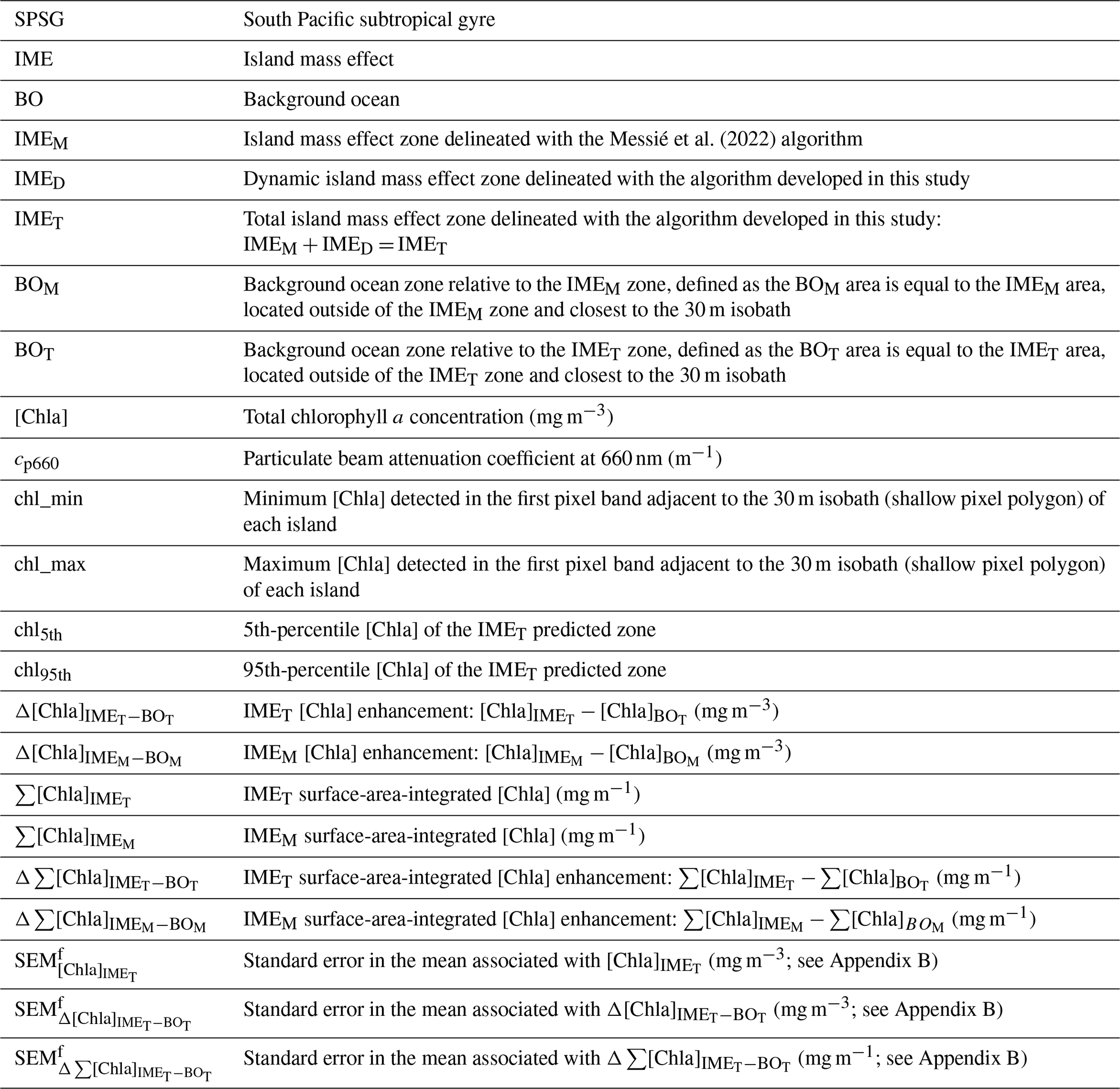

Table 1 Table of notations.

The limited accessibility to vast areas in the South Pacific Ocean makes ocean color remote sensing approaches well-suited for basin-scale studies of the IME. Using long-term averages of [Chla] from ocean color remote sensing data (July 2002 to June 2012), Gove et al. (2016) showed that the IME is a nearly ubiquitous phenomenon across the Pacific Ocean. The authors estimated the magnitude of IMEs by looking at changes in [Chla] within a ∼ 30 km wide band around each island's 30 m isobath, relative to BO reference pixels located just outside this band (Gove et al., 2013, 2016). In practice, this detection method uses the same quantitative approach as Doty and Oguri (1956) and accurately assesses the magnitude of the [Chla] enhancement associated with the IME as long as the BO reference pixels are outside the region affected by the IME. This assumption is reasonable for small islands (most islands in Gove et al., 2016, were smaller than a 30 km equivalent spherical diameter) and when using multi-year averages of [Chla] that tend to highlight only locations with permanent [Chla] enhancement (see below). A more recent basin-scale study of the IME aimed to capture more complex spatial heterogeneity around islands by defining a specific [Chla] contour to delineate the extent of the IME, allowing for the detection of the IME to extend further than 30 km away from the 30 m isobath (Messié et al., 2022).

Generally speaking, approaches for the detection of the IME from remotely sensed [Chla] require full or nearly full pixel data recovery over the entire study area for an accurate delineation of the extent of the IME. Messié et al. (2022) used yearly and monthly averages of 4 km spatial resolution [Chla] maps for their basin-scale estimation of the IME. While this temporal and spatial averaging enables the production of gapless [Chla] maps, it reduces the ability to detect fine-scale heterogeneity in space and time (Lee et al., 2018), only highlighting [Chla] enhancement observable at the same location over the time frame of the averaging period and therefore generally confined to regions directly adjacent to islands. Indeed, determining the spatial extent of the biological response of the IME and its effect on the ecology and bio-geochemistry of the adjacent oligotrophic ocean is challenging due to its spatial heterogeneity and the transient nature of phytoplankton responses to perturbations (Messié et al., 2020; Cassianides et al., 2020). Surface ocean properties, as observed by satellite sensors, are advected by wind and currents across a kilometer-wide pixel on a timescale of a few hours. Therefore, observations of the ocean using yearly averages only capture spatial patterns due to dominant winds and currents over this time frame, ignoring spatial and temporal heterogeneity caused by short-term wind and current variability. Thus, a more accurate quantification of IME extent and dynamics requires temporal averaging of satellite data over shorter timescales (e.g., to resolve mesoscale variability, up to 2 weeks) and tracking the evolution of IMEs over space and time using surface current data (Cassianides et al., 2020). Ideally, daily observations of the entire global ocean would provide the necessary temporal resolution to track IMEs. In reality, satellite measurements of the ocean surface in visible and near-infrared wavelengths are often obstructed by clouds or affected by sunglint, limiting the extent of data recovery at the necessary temporal scales.

Here, we present a method to increase satellite data recovery to improve the spatial and temporal resolution of satellite observations by merging products from up to five different satellite sensors and using an atmospheric correction that is less sensitive to glint and adjacency effects. These merged products reveal frequent occurrences of higher [Chla] patches that are detached from islands and advected offshore (referred to as “delayed IME” in Messié et al., 2020). The higher temporal resolution achieved allows for a more accurate estimation of [Chla] accumulation as a proxy for phytoplankton biomass accumulation (termed “blooms”) associated with IMEs. Building upon the work of Messié et al. (2022), we integrate modeled surface currents to develop a dynamic algorithm for the detection of the IME. We applied this algorithm to four island groups in the South Pacific Ocean (i.e., Rapa Nui, Society Islands, Samoa, and Fiji) over a 6-month period and show that accounting for detached patches significantly increases estimates of total [Chla] stocks associated with the IME in the area of study. This implies that the IME has a much larger impact on the oligotrophic ocean than previously estimated.

2 Method

2.1 Level-2 satellite product computation

The use of a single satellite sensor often results in maps with significant gaps in data due to intermittent cloud cover or glint (which depends on the satellite-specific viewing angle). To address this, we have adapted NASA Ocean Color's processing strategy to produce level-3 custom-made composite products from level-1A (L1A) top-of-atmosphere radiance. We merged data collected by three different sensor types (Moderate Resolution Imaging Spectroradiometer, MODIS; Visible Infrared Imaging Radiometer Suite, VIIRS; and Ocean and Land Colour Instrument, OLCI) on board up to six polar-orbiting satellites (Aqua, Terra, SNPP, JPSS1, Sentinel-3A, and Sentinel-3B). By taking advantage of their different overpass times, swaths, and viewing geometry, we decreased the impact of clouds and glint on data recovery. Additionally, we applied the POLYMER atmospheric correction (Steinmetz et al., 2011) to further improve data recovery in areas impacted by glint and adjacency effect (e.g., close to shore and clouds). POLYMER is an atmospheric correction based on a spectral matching method to decompose the top-of-atmosphere (TOA) signal into an atmospheric model and an ocean reflectance model. A three-term polynomial fit is used to model the atmospheric reflectance, with the first term accounting for non-spectral scattering such as sunglint and the last term accounting for adjacency effect from clouds and white surfaces (Steinmetz et al., 2011). By utilizing the entire TOA spectrum and accounting for adjacency effects and residual glint in its polynomial fit terms, this method improves the retrieval of high-quality data around clouds and from pixels affected by sunglint compared to standard atmospheric correction methods (Frouin et al., 2009, 2012). The POLYMER atmospheric correction was initially developed for the Medium Resolution Imaging Spectrometer (MERIS) sensor but was adapted to produce consistent ocean color products between MODIS, VIIRS, and OLCI sensors, among others (Steinmetz and Ramon, 2018).

Most operational level-3 products are available at spatial resolutions of 4 or 9 km. While this resolution is usually sufficient to capture important mesoscale spatial features in the open ocean, it does not resolve sub-mesoscale features like fronts, small eddies, and filaments around islands. Additionally, bottom reflectance in coastal waters prevents data recovery closer than 4 or 9 km from shore at these spatial resolutions. Moreover, it is a common practice in coastal studies to remove at least one neighboring pixel around shallow areas to limit the impact of adjacency effects and ensure no contamination from bottom reflectance. Therefore, the closest data recovered with a 4 km spatial resolution are most often centered at least 6 km away from the 30 m isobaths. However, most islands in the ocean are smaller than 2 km². For instance, the median island area in the 2593 km × 2593 km region analyzed around the Fiji Archipelago is ∼ 0.06 km² with ∼ 86 % of all islands smaller than 2 km². Therefore, having the closest pixel 6 km away from shore and a pixel size that is at least twice the size of ∼ 86 % of islands limits our ability to accurately quantify their IME (see for example Niue, Fig. A2). With the approach presented here, we can maximize data recovery close to shore while keeping the nominal resolution of 1 km of the operational MODIS and VIIRS level-2 (L2) products. Ideally, we would produce this type of multi-satellite composite for the entire Pacific Ocean, but we had to limit our study area to four case studies around islands of interest due to computational and data storage capacity limitations. In each case, the maps were large enough (i.e., >1200 km × 1200 km area) to capture the full extent of the IME around the group of islands studied and were limited to a maximum size of a 2600 km × 2600 km area.

All analyses for this study were conducted using the University of Maine's high-performance Linux computing cluster following the processing pipeline shown in Fig. A1. We downloaded level-1 (L1A) top-of-atmosphere radiance of MODIS Aqua, MODIS Terra, VIIRS SNPP, and VIIRS JPSS1 via NASA's common metadata repository application programming interface (CMR API, 2024) and the resampled 1 km spatial resolution OLCI S3A and OLCI S3B data via Copernicus Data Space Catalogue API (2024) using the Python download utility “getOC” (see the GitHub reference of Haëntjens and Bourdin, 2017). We built two sets of satellite data. We downloaded the first set of images along the entire Tara Pacific transect (May 2016 to October 2018; see Gorsky et al., 2019; Lombard et al., 2023) and used it to compute sensor-specific calibration coefficients based on correlation with continuous in situ data (see Sect. 2.2). We refer to it as the “calibration dataset”. The second set of images, referred to as the “study dataset”, consisted of 6-month-long time series of satellite images in the vicinity of islands of interest. We processed all downloaded L1A images into atmospherically corrected level-2 remote sensing reflectance (R_rs) data using the POLYMER algorithm (version v4.17beta2; Steinmetz, 2023) and ancillary data from the European Centre for Medium-Range Weather Forecasts reanalysis model version 5 (i.e., ERA5). We removed poor-quality data pixels by applying the flags and recommendations of POLYMER (see POLYMER flags, 2024). For comparison, we also generated the standard NASA R_rs using the atmospheric correction of SeaDAS (i.e., “l2gen”) using the Ocean Color Science Software (OCSSW) V2022.3, and applying the Ocean Color default flags (see NASA OBPG flags, 2024). Subsequently, we projected each satellite image of the study dataset onto the same equally spaced 1 km spatial resolution plate carrée reference grid specific to each studied region using nearest-neighbor interpolations from Python's SciPy library. We estimated [Chla] from all POLYMER and l2gen R_rs data using the OCx algorithm (i.e., chl_ocx; O'Reilly and Werdell, 2019) and the CI-OCx blended algorithm (i.e., chlor_a; Hu et al., 2019; O'Reilly and Werdell, 2019).

2.2 In situ data and match-ups

We calibrated remote sensing products to minimize inter-sensor variability and biases using in situ data collected during the Tara Pacific Expedition (Gorsky et al., 2019; Lombard et al., 2023). We measured hyperspectral absorption (a) and attenuation (c) quasi-continuously near islands with a SeaBird ac-s spectrophotometer mounted in an underway flow-through system. We computed particulate absorption and attenuation coefficients (i.e., a_p and c_p) by referencing these sensor measurements to hourly samples taken through a 0.2 µm filter (Dall'Olmo et al., 2009; Slade et al., 2010; Boss et al., 2019). Particulate beam attenuation at 660 nm (c_p660) was used as a proxy for particulate organic carbon (Gardner et al., 2006; Cetinić et al., 2012). We estimated absorption specific to Chla-containing particles using the line height of the a_p peak at 676 nm (a_p676LH; Boss et al., 2013). We collected surface samples daily around 10:30 local time for pigment analysis via high-pressure liquid chromatography (HPLC; see Gorsky et al., 2019; Lombard et al., 2023). We then estimated [Chla] from a_p by applying the well-constrained linear relationship between the logarithm of a_p676LH amplitude and the logarithm of total [Chla] estimated from HPLC (Fig. B2a).

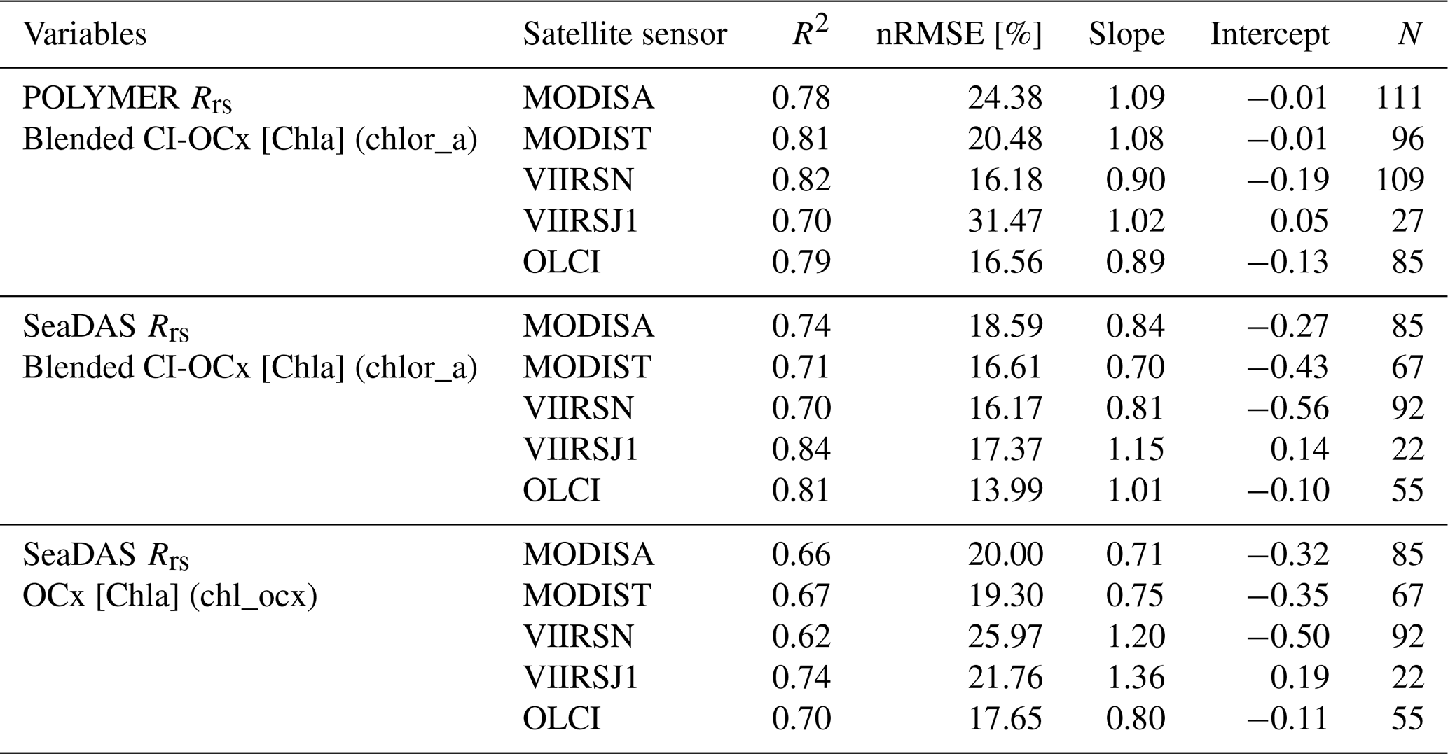
We performed match-ups between the calibrated [Chla] estimated from the underway system and the [Chla] estimated from satellites to choose the best algorithm (i.e., least noisy or biased) to compute [Chla] from satellite R_rs. We matched three different [Chla] products (i.e., chlor_a_polymer, chl_ocx_seadas, chlor_a_seadas) with the calibrated [Chla] estimated from the underway system following Bailey and Werdell (2006). We extracted and averaged underway [Chla] measurements within a ±3 h period of each satellite overpass (i.e., Aqua and SNPP, 13:30; Terra, 10:30; Sentinel-3A and Sentinel-3B, 10:00; JPSS1, 14:20 local time at the Equator) and satellite data from the 25 closest pixels to underway data locations. We computed median coefficients of variation in R_rs for bands between 412 and 555 nm and for the aerosol optical thickness at 865 nm for each match-up and tested several homogeneity thresholds and the minimum number of unmasked pixels to maximize the number of valid match-ups without introducing noise to the in situ satellite correlations (Bailey and Werdell, 2006). Only match-ups with a minimum of seven unmasked pixels and coefficients of variation lower than 0.15 were kept (Fig. B2b, c, and d). We compared the parameters of the robust linear regressions of valid match-ups to choose the best [Chla] derivation methods (Table B1). We found 33 % more valid match-ups with [Chla] computed using POLYMER R_rs (N=428) than valid match-ups with [Chla] computed using SeaDAS R_rs (N=321). [Chla] computed with the blended CI-OCx using POLYMER R_rs showed, on average, the highest coefficient of determination (${\stackrel{\mathrm{‾}}{R^{\mathrm{2}}}}_{\text{chlor\_a\_polymer}}=\mathrm{0.78}\pm \mathrm{0.05}$), slopes closest to 1 (${\stackrel{\mathrm{‾}}{\mathrm{slope}}}_{\text{chlor\_a\_polymer}}=\mathrm{0.99}\pm \mathrm{0.10}$), and intercepts closest to 0 (${\stackrel{\mathrm{‾}}{\mathrm{intercept}}}_{\text{chlor\_a\_polymer}}=-\mathrm{0.06}\pm \mathrm{0.10}$) when compared to in situ [Chla]. In contrast, the normalized root mean square error in the correlation between in situ [Chla] and [Chla] computed with the blended CI-OCx using POLYMER R_rs (${\stackrel{\mathrm{‾}}{\mathrm{nRMSE}}}_{\text{chlor\_a\_polymer}}=\mathrm{21.81}\pm \mathrm{6.34}$ %) was higher than with the other two [Chla] values computed using SeaDAS R_rs (${\stackrel{\mathrm{‾}}{\mathrm{nRMSE}}}_{\text{chlor\_a\_seadas}}=\mathrm{16.55}\pm \mathrm{1.70}$ % and ${\stackrel{\mathrm{‾}}{\mathrm{nRMSE}}}_{\text{chl\_ocx\_seadas}}=\mathrm{20.94}\pm \mathrm{3.18}$ %). Considering the smaller bias (slope closer to 1 and intercept closer to 0) and better data recovery (higher number of valid match-ups) associated with the computation of [Chla] with the blended CI-OCx algorithm applied on POLYMER R_rs, we choose this method for the rest of the analysis to minimize differences between sensors while maximizing valid pixel recovery. Despite the well-documented degradation of the MODIS sensor on board the Terra satellite and its potential impact on climate studies (Lyapustin et al., 2014; Xiong et al., 2019; Xiong and Butler, 2020), our analysis found no significant indication of reduced data quality in [Chla] estimates derived from MODIS Terra R_rs. Correlations between in situ [Chla] and MODIS Terra-derived [Chla] showed performance metrics (R², nRMSE, slope, and intercept) comparable to those of other satellite sensors included in this study (Table B1 and Fig. B2 b, c, and d). These findings suggest that the extensive correction and calibration efforts applied to MODIS Terra data effectively mitigate the impacts of solar diffuser degradation, changes in scan mirror reflectance, and increased polarization sensitivity (Lyapustin et al., 2014). As a result, MODIS Terra data can be reliably incorporated into the multi-satellite merged product used in this study.

2.3 Level-3 multi-satellite product merging

We followed a similar merging strategy to that of Copernicus' multi-satellite Global Ocean Colour processor (i.e., GlobColour): each sensor's satellite product was derived separately before merging them (Garnesson et al., 2019), rather than the strategy of the Ocean-Colour Climate Change Initiative (i.e., OC-CCI), which merges reflectances before calculating the products (Sathyendranath et al., 2019). This method offers two important advantages: (1) it does not require any band-shifting procedures to merge R_rs between sensors with different spectral bands, and (2) it benefits from sensor-specific algorithm coefficients that account for variability in R_rs across sensors to produce consistent products (Garnesson et al., 2019). To improve consistency and minimize the differences across satellite sensors, we individually calibrated the [Chla] data from each sensor with the underway in situ [Chla] measurements (using parameters from their respective robust linear regressions; see Table B1) to produce “calibrated” products before merging them. This nudging method reduced the inter-satellite variability and improved the spatial smoothness of the binned products. Since [Chla] was calibrated to in situ data, the bias associated with the estimation of [Chla] from each satellite was centered and likely reduced to the bias of in situ data. For each study area, we binned the calibrated data temporally to reconstruct full satellite images. Time series of 8 d periods were the smallest temporal binning we could achieve to recover nearly full satellite images in all the studied regions for 6-month-long time series. Before computing the merged products of a given 8 d period and a given region, we grouped all re-projected level-2 images and removed outliers (see Appendix C). To minimize the weight of outliers on the level-3 end products, the binning was performed with medians instead of averages. We produced a 6-month-long time series of level-3 8 d medians of [Chla] for each of the four case studies presented here. Each case-study region was centered geographically on an island sampled during the Tara Pacific Expedition, and each 6-month time series was centered temporally on the day of in situ sampling (Gorsky et al., 2019; Lombard et al., 2023). We propagated errors associated with [Chla] estimation, nudging, and merging throughout each step to represent the final [Chla] uncertainty denoted as the standard error in the mean (i.e., SEM) of the merged product (${\mathrm{SEM}}_{[\mathrm{Chla}{]}_{\mathrm{IME}}}^{\mathrm{f}}$; see Appendix B). We used this final uncertainty to determine if the [Chla] enhancement associated with an IME was significant or not.

2.4 Island mass effect detection

2.4.1 Bathymetry, island, and submerged reef databases

We created masks at 1 km spatial resolution denoting land (land mask) and areas shallower than 30 m depth (shallow mask) for the studied areas using the General Bathymetric Chart of the Oceans (GEBCO) database (GEBCO Bathymetric Compilation Group, 2022). Since a large number of islands and reefs are smaller than the spatial resolution of the GEBCO database (i.e., 15 arcsec corresponding to 463 m at the Equator), we utilized the 30 m spatial resolution global island database (Sayre et al., 2019, 2020) to refine the land and shallow masks for the study areas. We then extended the shallow mask by one additional pixel to ensure all shallow pixels are masked. Subsequently, we merged the global island database and the submerged reef database from Messié et al. (2022) into a single database. To ensure accuracy, we automatically verified all island centroids to confirm their alignment with a land pixel on the land mask and to ensure their associated land polygon was not significantly smaller than the reported island area in the global island database. Similarly, we automatically checked all submerged reef centroids to confirm their alignment with a shallow mask pixel and to ensure their associated shallow-mask polygons were not significantly smaller than the reported reef area in the Messié et al. (2022) database. We manually corrected any discrepancies that were identified when comparing to the bathymetry data and saved the corrections for reference. For simplicity, the term “islands” in this study also refers to submerged seamounts or reefs shallower than 30 m depth.

2.4.2 IME contour delineation

The [Chla] contour value delineating the IME was determined in three successive steps to dynamically detect detached IME patches. The first step used the method from Messié et al. (2022) to detect IMEs on each 8 d composite map of the time series (see step 1 of Fig. 1a). This method defines the [Chla] contour value with an iterative process starting from the highest (chl_max) to the lowest [Chla] (chl_min) values detected one pixel away from the 30 m isobath of each island and ending when a set of specified conditions is met. These conditions include (1) when [Chla] values fall below chl_min, (2) when the IME mask touches the domain borders or a continent masks, and (3) when regions with [Chla] exceeding 80 % of the chl_max are detected farther than 150 km away from the 30 m isobath. This 150 km threshold was set to allow for the detection of water masses that were detached from an island and advected offshore (denoted “detached IMEs”) but, at the same time, to prevent potential bias by accounting for non-IME-related [Chla] variability far from the island. We observed that this algorithm performed well when the IME is directly adjacent to the 30 m isobath of an island and when the IME is spatially homogeneous, with the highest [Chla] values typically located near the island and decreasing with distance from shore (similar to the IME detected with monthly or yearly satellite averages; Messié et al., 2022). Therefore, this method is valuable as the first step for detecting the strongest IME signal that surrounds an island, referred to in this study as IME_M (step 1 of Fig. 1a). However, this approach underestimates the entire extent of an IME when applied to 8 d [Chla] products because it fails to detect elevated [Chla] patches that have been detached from their originating IME or when pixels with $\left[\mathrm{Chla}\right]>\mathrm{0.8}\times \text{chl\_max}$ were detected more than 150 km from the island of origin. Detached IMEs, typically comprised of dynamic filaments and eddies that are quickly advected away from islands, are detectable on 8 d averaged satellite products but often not captured using monthly or yearly averages such as the products used by Messié et al. (2022). We therefore extended the method proposed by Messié et al. (2022) by adding another set of detection protocols, here called step 2 and step 3. We utilized modeled daily surface currents (i.e., global ocean ensemble physics reanalysis products provided by Copernicus Marine Services; European Union-Copernicus Marine Service, 2019) to predict the general locations of IME patches that detach from islands (step 2 of Fig. 1). For clarity, we refer to the detached IME area obtained with this approach as IME_D (step 3 of Fig. 1). The sum of both the IME_M and IME_D areas (i.e., total IME) is referred to as IME_T. The following sequence was applied to detect IMEs in each 8 d median composite of the time series (Fig. 1):

• Step 1 is the detection of IME_M (Messié et al., 2022, Fig. 1a).

• Step 2 is the prediction of the general location of IME_D by applying the average current u and v vectors from the previous 8 d period ($t=-\mathrm{1}$) to the location of IME_T detected at $t=-\mathrm{1}$ (Fig. 1d). When step 2 is performed on the first 8 d median of the time series (t=0), the surface current at t=0 is applied to the IME_M detected at t=0 instead (Fig. 1b).

• Step 3 is the delineation of IME_D and IME_T using a second round of [Chla] value iteration, ranging from the 95th to the 5th percentiles of [Chla] measured within the predicted zone and only keeping the patches that overlap with the predicted zone location as explained below.

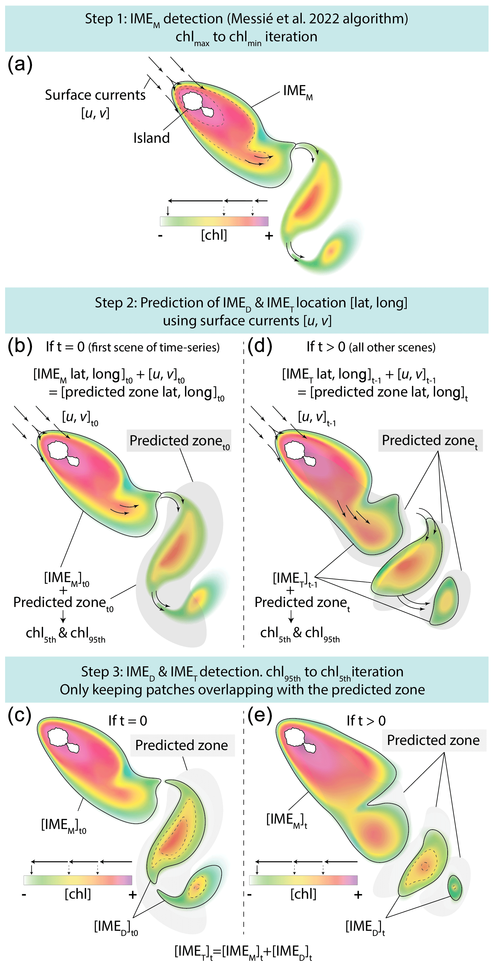
Figure 1 Island mass effect detection method. (a) Step 1: [IME_M]${}_{t_{\mathrm{0}}}$ detection following the method from Messié et al. (2022). (b) Step 2 at t=0 (first image of the time series): prediction of the detached IME ([IME_D]${}_{t_{\mathrm{0}}}$) location applying t₀ surface currents ([u,v]${}_{t_{\mathrm{0}}}$) to the [IME_M]${}_{t_{\mathrm{0}}}$ location. (c) Step 3 at t=0: detached IME contour detection ([IME_D]${}_{t_{\mathrm{0}}}$) iterating from the 95th to the 5th percentile of [Chla] (chl_95th and chl_5th respectively) detected within the [IME_M]${}_{t_{\mathrm{0}}}$ and the t₀ predicted zone. (d) Step 2 at t>0 (rest of the time series): prediction of the [IME_D]_t location applying t₋₁ surface currents ([u,v]${}_{t_{-\mathrm{1}}}$) to the total IME location detected in the previous image ([IME_T]${}_{t_{-\mathrm{1}}}$). (e) Step 3 at t>0: [IME_D]_t contour detection iterating from chl_95th and chl_5th detected within the [IME_T]${}_{t_{-\mathrm{1}}}$ and the t predicted zone.

Step 3 of the detection involves a second round of [Chla] iteration, which is based on the IME_M detection method but adapted to the higher-resolution satellite composites. First, we modified the detection of the [Chla] range, defining the range of iteration for a given IME, to better capture the dynamic range in [Chla] of the entire IME while avoiding potential biases in pixels adjacent to the island due to bottom reflectance and adjacency effect. We performed the [Chla] iteration from the 95th to the 5th [Chla] percentiles of the entire predicted zone (chl_95th and chl_5th) instead of performing the [Chla] iteration from chl_max to chl_min of the first pixel band around the 30 m isobath of each island. Additionally, the iteration step size was automatically defined to always correspond to 30 [Chla] steps within the [Chla] range of the entire predicted zone (from chl_95th to chl_5th). The number of [Chla] iteration steps (i.e., 30 iterations) was optimized by trial and error to better detect the IME around Rapa Nui, where the [Chla] dynamic range is the lowest and where a small change in the [Chla] contour has the most impact on the IME surface detected. Similarly to the IME_M detection, once the [Chla] contour value was found, the iteration was performed again, starting at the preceding iteration but with an iteration step size divided by 10 in order to delineate the IME patch more accurately. As a result, the [Chla] iteration step value ranged from 10⁻⁴ to 10⁻¹ mg m⁻³ which, in low-dynamic-range regions, is smaller than the 10⁻³ mg m⁻³ step value used in Messié et al. (2022) and smaller than the accuracy of absolute [Chla] retrieval from satellites (10⁻¹ mg m⁻³, discussed below). This smaller [Chla] iteration step value improved the performance of the detection algorithm around islands in regions with a very low dynamic range in [Chla] (e.g., Rapa Nui). We also modified the conditions to stop the [Chla] iteration, removing the condition that stopped the [Chla] iteration when pixels with $\left[\mathrm{Chla}\right]>\mathrm{0.8}\times \text{chl\_max}$ are located more than 150 km away from the studied island to allow for the detection of a detached IME further than 150 km away from the island (i.e., condition number 3; Messié et al., 2022). Additionally, instead of stopping the [Chla] iteration when the IME touched the domain border, the IME was considered to be exiting the domain, and the iteration was stopped when, for a given [Chla] contour, more than 25 % of the predicted pixel location overlapped with a chlorophyll patch touching the border. This modification improved detection of the IME by tolerating a small proportion of the IME patch to be advected near the domain border while still stopping the iteration when the [Chla] contour becomes too low and includes features that are not part of the IME. We also added a condition to stop the IME_D [Chla] iteration when the IME_D [Chla] contour intersected an IME_D contour associated with another island. Finally, as in Messié et al. (2022), the BO reference zones associated with each IME zone (i.e., IME_M, IME_D, and IME_T) were defined as the area equal to the size of the corresponding IME zone but located outside of the IME zone, closest to the shallow mask (i.e., BO zone associated with IME_M denoted BO_M and BO zone associated with IME_T denoted BO_T, Table 1). We computed surface-area-integrated [Chla] as a proxy for surface phytoplankton biomass integrated over the entire IME and BO zones in two-dimensional metric tons of chlorophyll a (t m⁻¹) by summing the [Chla] of each pixel within the IME and BO zones multiplied by the area of that pixel:

$$\begin{array}{}\text{(1)}& \sum [\mathrm{Chla}{]}_{\mathrm{IME}}=\sum _{n=\mathrm{1}}^{N_{pixe{l}_{\mathrm{IME}}}}[\mathrm{Chla}{]}_n\times {\mathrm{area}}_{{\mathrm{pixel}}_n}.\end{array}$$

The difference in average [Chla] and $\sum [\mathrm{Chla}{]}_{{\mathrm{IME}}_{\mathrm{T}}}$ between the IME and the corresponding BO reference zone was computed to estimate the biomass increase associated with an IME relative to the BO (i.e., $\mathrm{\Delta }[\mathrm{Chla}{]}_{{\mathrm{IME}}_{\mathrm{T}}-{\mathrm{BO}}_{\mathrm{T}}}$ and $\mathrm{\Delta }\sum [\mathrm{Chla}{]}_{{\mathrm{IME}}_{\mathrm{T}}-{\mathrm{BO}}_{\mathrm{T}}}$ respectively). The [Chla] enhancement attributed to a given IME was deemed significant when both the mean and integrated values were above their uncertainty, e.g., $\mathrm{\Delta }[\mathrm{Chla}{]}_{{\mathrm{IME}}_{\mathrm{T}}-{\mathrm{BO}}_{\mathrm{T}}}-{\mathrm{SEM}}_{\mathrm{\Delta }[\mathrm{Chla}{]}_{{\mathrm{IME}}_{\mathrm{T}}-{\mathrm{BO}}_{\mathrm{T}}}}^{\mathrm{f}}>\mathrm{0}$ or $\mathrm{\Delta }\sum [\mathrm{Chla}{]}_{{\mathrm{IME}}_{\mathrm{T}}-{\mathrm{BO}}_{\mathrm{T}}}-{\mathrm{SEM}}_{\mathrm{\Delta }\sum [\mathrm{Chla}{]}_{{\mathrm{IME}}_{\mathrm{T}}-{\mathrm{BO}}_{\mathrm{T}}}}^{\mathrm{f}}>\mathrm{0}$. Examples of IME zones detected on the 6-month-long map time series around Fiji–Tonga and Samoa–Niue (Figs. 2 and 3; Supplement Animations S1 and S2; Bourdin, 2025) show contours outlining the IME_M (i.e., red contours), the extension of the algorithm to detect the IME_D (i.e., blue contours), and their associated BO_T zones (i.e., white circles). The same analysis was performed around Rapa Nui and the Society Islands and is accessible in Bourdin (2025).

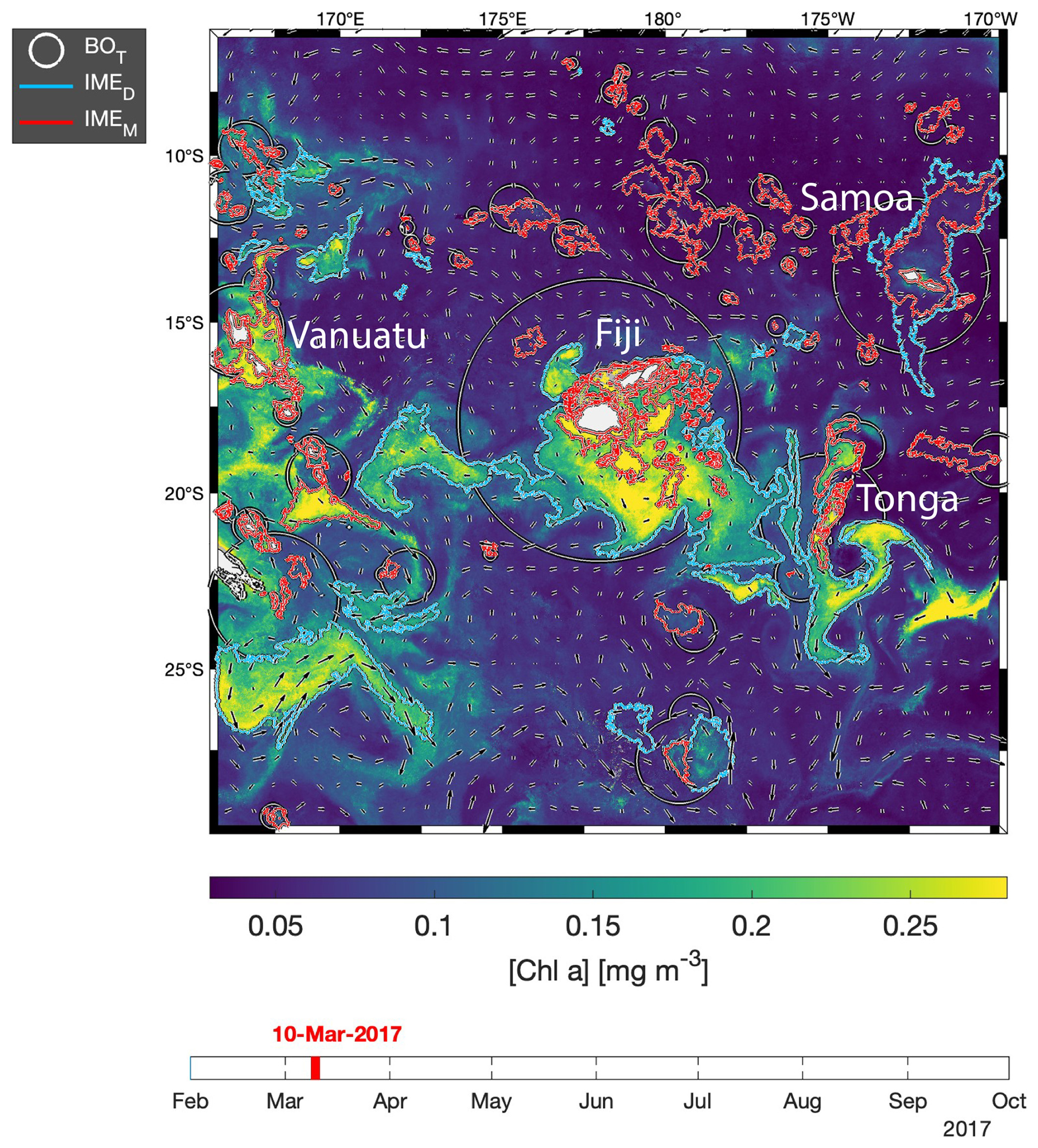
Figure 2 Snapshot of 6-month-long time series of 8 d multi-satellite composites of the total chlorophyll a concentration ([Chla]) around the Fiji and Tonga archipelagos. The IME_M (Messié et al., 2022) contours are delineated in red, the IME_D contours added in this study are delineated in blue, and the BO_T zones associated with each IME_T area are delineated with white circles. Overlaid arrows represent modeled surface current. Entire 6-month animated time series are accessible in the Supplement (Animation S1) or in Bourdin (2025).

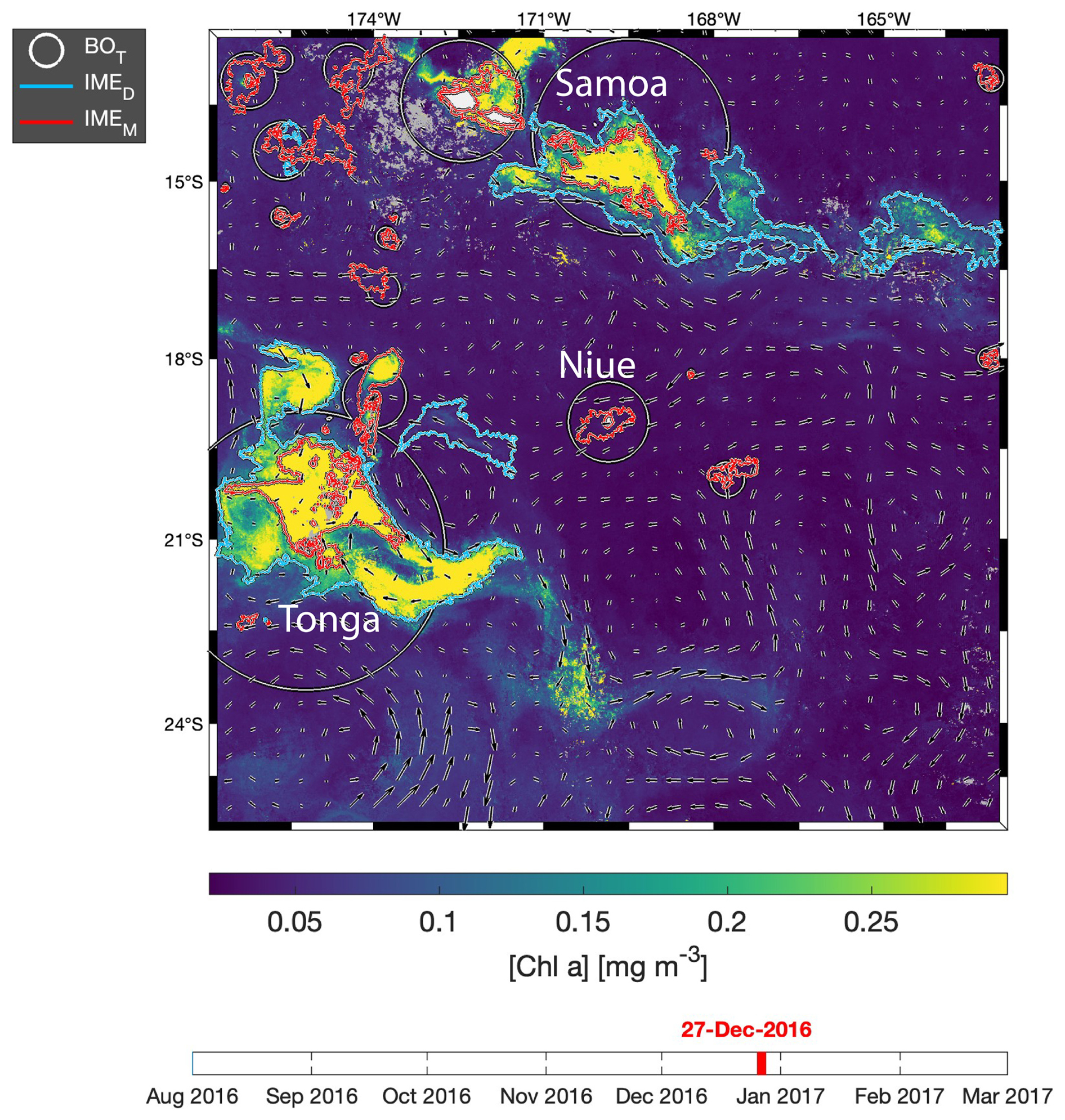
Figure 3 Snapshot of 6-month-long time series of 8 d multi-satellite composites of the total chlorophyll a concentration ([Chla]) around Samoa, Tonga, and Niue. The IME_M (Messié et al., 2022) contours are delineated in red, the IME_D contours added in this study are delineated in blue, and the BO_T zones associated with each IME_T area are delineated with white circles. Overlaid arrows represent the modeled surface current. Entire 6-month animated time series are accessible in the Supplement (Animation S2) or in Bourdin (2025).

2.4.3 Detecting the IME around neighboring islands

In the case of neighboring islands, it is important to define which island, among a group of islands within a common IME_M patch, contributes the most to the IME_M (referred to as the “lead island”). In Messié et al. (2022), the lead island was defined as the island with the highest chl_min value detected on the first pixel band adjacent to its shallow-mask polygon. In our study, the 8 d median composite product maps are more spatially heterogeneous than monthly or yearly averages used in Messié et al. (2022), and therefore chl_min values may not be the best indicator to assign a lead island. Moreover, the first pixel band adjacent to the shallow mask, from which the chl_min value is extracted, is the most likely to be impacted by the adjacency effect and bottom reflectance, leading to potential misassignment of the lead island. For example, the 6-month map time series around Fiji shows regions of enhanced [Chla] that have been advected in different directions around the archipelago, with the largest bloom always centered on Fiji's two largest islands (i.e., Viti Levu at 10 912 km² and Vanua Levu at 5817 km²; Fig. 2 and Supplement Animation S1). When applying the IME_M criteria, the lead island was assigned to smaller islands (e.g., Koro Island and Yalewa Kalou Island, which have a surface area of 105 km² and at 0.2 km², respectively) or to a 20 km² submerged reef in 19 % of the realizations in this time series. Likewise, when applying the IME_M criteria on the Society Islands' IME, the lead island was assigned to small islands in 24 % of the 8 d frames in the time series, although the bloom was always centered on Tahiti. Based on observations of the time series of [Chla] maps, we found that, for large islands (>100 km²), the largest IMEs, in terms of the area and magnitude of [Chla], are generally located around islands with the largest land area. For that reason, in our dynamic model the lead island was reassigned after the IME_M detection (step 1 of Fig. 1a) following a different ranking (see below), which was also later used as the order of detection of IME_D (step 3 of Fig. 1). All islands of a specific study region were first sorted by 100 km² increments of land area categories (smaller than 100 km², between 100 and 200 km², etc.), and then within each category they were further sorted by increments of 10 km² 30 m isobath area sub-categories (representing the reef area). Thus, land area is ranked higher than reef area only when islands are larger than or equal to 100 km². We further ranked islands within each land area category and reef area sub-category using their IME intensity based on chl_95th values, rounded to the closest 0.1 mg m⁻³. Finally, islands of a similar rounded land area, rounded reef area, and rounded chl_95th were ranked by their calculated IME_M area. The IME_T detection was performed following this ranking order; thus, for a given IME_T zone encompassing multiple islands, the lead island was defined as the top-ranked island in the IME_T zone. Once all IME_T detections were performed, the lead islands assigned by this ranking were verified to ensure that, among all islands associated with a given IME_T patch, the lead island was indeed selected as the first island in the ranking previously defined. Considering the complexity of the currents around archipelagos, we acknowledge that although a single lead island was assigned to a given IME_T, the enhancement in [Chla] associated with IMEs could originate from the influence of multiple islands. For instance, the IME associated with Fiji was a combination of IMEs of all islands and submerged reefs of the archipelago, which was also often mixed with the substantial IME influence of the Tonga Archipelago. Therefore, IMEs of all islands and reefs associated with archipelagos were combined into an “archipelago IME”, such as the “Fiji–Tonga” IME example (Fig. 2), to track the evolution of the combined IME over the 6-month time series produced (i.e., 88 islands and 140 submerged reefs; Fig. 4). Likewise, the IME_T associated with Samoa encompassed the IMEs of Savaii, Upolu, and Tutuila and all the other small islands and reefs contained within the IME_T patch detected around the archipelago (i.e., 7 islands and 38 submerged reefs; Fig. 5). The IME around the Society Islands in French Polynesia was also combined into one large IME that encompassed the Society Islands themselves, the Tuamotu Archipelago, and all small islands and reefs located in the large IME zone detected around Tahiti (i.e., 176 islands and 34 submerged reefs; Fig. E2). The IME_T associated with Rapa Nui encompassed Rapa Nui and Sala y Gómez and two submerged reefs (Fig. E1).

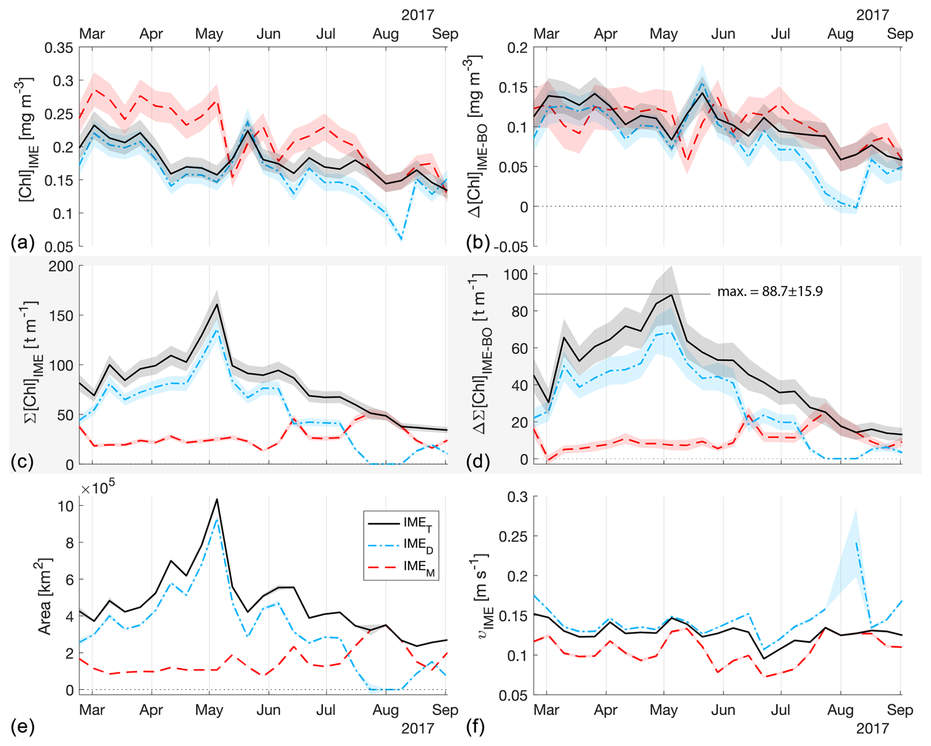
Figure 4 The 6-month-long time series of satellite-derived IME properties of the IME zones (IME_M, dashed red line; IME_D, dash-dotted blue line; IME_T, solid black line) detected around the Fiji and Tonga archipelagos combined. (a) Average chlorophyll a concentration within the IME zones ([Chla]_IME), (b) difference in average [Chla] between each IME zone and their respective BO zones (Δ[Chla]_IME−BO), (c) IME surface-area-integrated chlorophyll a (∑[Chla]_IME), (d) difference in IME and BO surface-area-integrated chlorophyll a ($\mathrm{\Delta }\sum [\mathrm{Chla}{]}_{\mathrm{IME}-\mathrm{BO}}$), (e) IME zone area, and (f) surface current velocity.

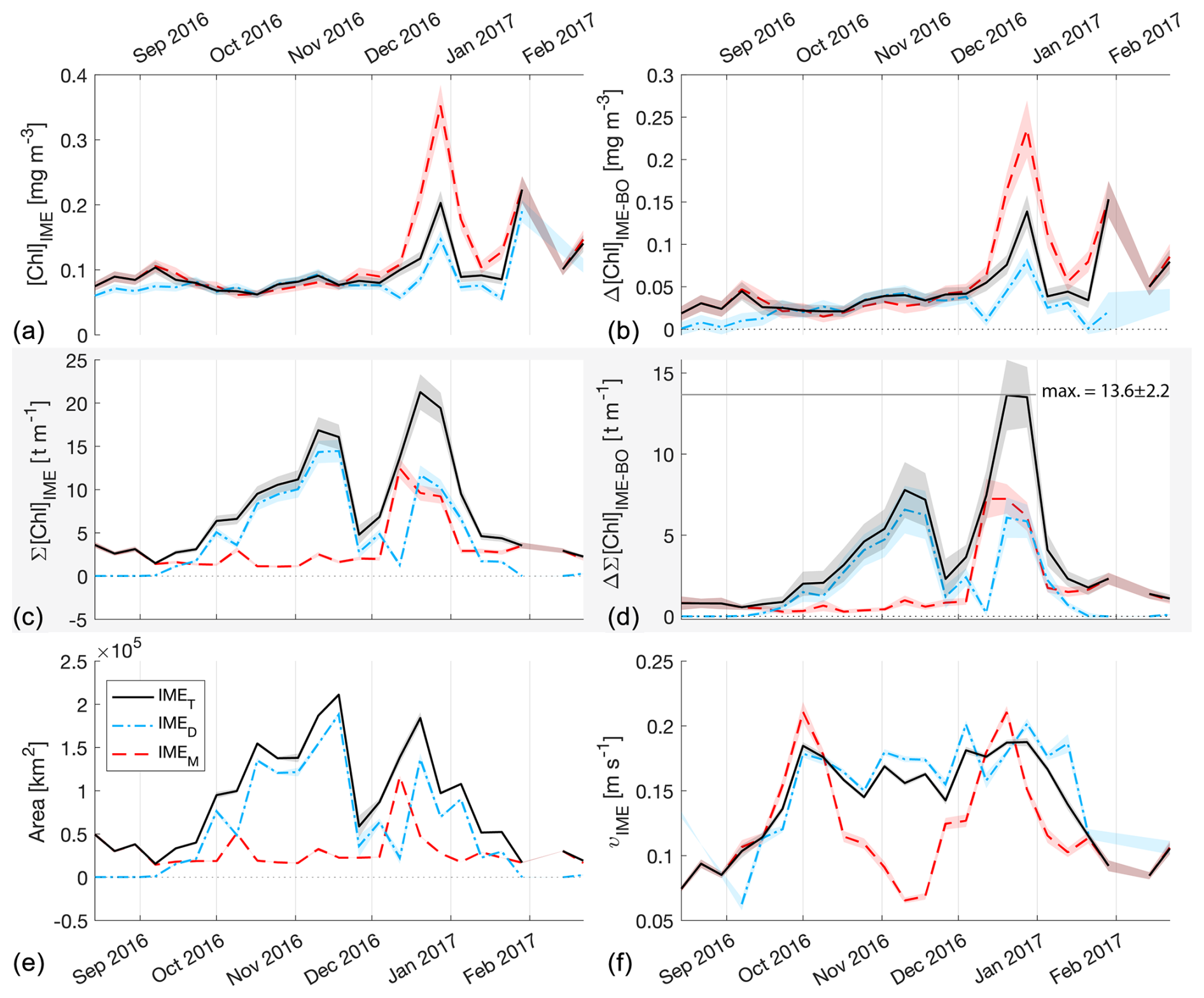
Figure 5 The 6-month-long time series of satellite-derived IME properties of the IME zones (IME_M, dashed red line; IME_D, dash-dotted blue line; IME_T, solid black line) detected around Samoa (Savaii, Upolu, and Tutuila). (a) Average chlorophyll a concentration within the IME zones ([Chla]_IME), (b) difference in average [Chla] between each IME zone and their respective BO zones (Δ[Chla]_IME−BO), (c) IME surface-area-integrated chlorophyll a (∑[Chla]_IME), (d) difference in IME and BO surface-area-integrated chlorophyll a ($\mathrm{\Delta }\sum [\mathrm{Chla}{]}_{\mathrm{IME}-\mathrm{BO}}$), (e) IME zone area, and (f) surface current velocity.

3 Assessment

3.1 Benefit of multi-sensor composites

The observation and tracking of water masses in the ocean from space are challenging due to glint and clouds that significantly reduce the amount of data recovered from satellite ocean color sensors. Furthermore, even without clouds or glint, uncertainties associated with satellite retrieval remain substantial, mainly due to atmospheric gases (Gilerson et al., 2022). This impact is even larger in oligotrophic and ultra-oligotrophic regions, where less light is reflected back to the satellites by the ocean in comparison to the atmosphere. Merging data from multiple satellites with different overpass times and viewing angles offers several advantages: (1) changing cloud coverage over time may allow for zones masked by clouds in the morning to be visible in the afternoon; (2) observing the ocean from varying viewing angles improves data recovery by minimizing the impact of sunglint; (3) assuming no bias, combining data from sensors with different inherent uncertainties likely reduces the overall uncertainty in the merged product; and (4) as atmospheric properties (other than clouds) change over time, merging data from multiple overpass times can further decrease the relative uncertainty in the final product. Moreover, the correction of the adjacency effect and glint by the POLYMER atmospheric correction further increases data recovery and reduces uncertainties around clouds and in glint-impacted areas. By merging products from multiple satellites, we maximized the amount of data available at a given time and location (∼ 10 measurements per pixel on average for a given 8 d period). The recovery of sufficient data for binning was critical for identifying and removing outliers and obtaining smooth level-3 products. This method allowed for a gapless and smooth coverage of the zones analyzed during a 6-month time series at an 8 d frequency and therefore improved the detection of sub-mesoscale currents, filaments, and eddies associated with the IME.

3.2 IME detection algorithm refinement

Time series of remote sensing maps (Bourdin, 2025) and their snapshots (Figs. 2, 3) reveal the complexity of currents around islands and the rather chaotic advection patterns of the IME into the open ocean and between islands. The four case studies were located in the South Pacific subtropical gyre (SPSG), where geostrophic currents are low and mesoscale and sub-mesoscale currents interact with island topography from variable directions. In this region, the “upstream” sides of islands also show enhanced [Chla], which suggests IME water masses are advected in all directions around islands (e.g., Fig. A2). Under these conditions and contrary to the assumption in Messié et al. (2022), there are generally no strict upstream pixels directly adjacent to an island. Consequently, defining the lower end of the [Chla] iteration as the minimum [Chla] detected in the first pixel band around the shallow pixel mask may result in an overestimation of the lower threshold of the [Chla] iteration and thus an underestimation of the IME area. Therefore, to better capture the local range in [Chla] and to avoid a potential remaining impact of adjacency effect and bottom reflectance on satellite retrievals, we extracted the range of the [Chla] iteration from the entire predicted zone of the IME location. In addition, to improve robustness and reduce sensitivity to noise, we used the 95th to the 5th percentiles instead of the maximum and minimum [Chla] values. By design, all IME [Chla] values were higher than the [Chla] of their respective BO zones; however, while the mean [Chla] values of all IME_T zones were significantly higher than their BO_T counterparts (i.e., $\mathrm{\Delta }[\mathrm{Chla}{]}_{{\mathrm{IME}}_{\mathrm{T}}-{\mathrm{BO}}_{\mathrm{T}}}-\mathrm{uncertainty}>\mathrm{0}$; Figs. 5, 4, E1, E2), IME_M [Chla] values were not significantly higher than their BO_M counterparts in several occurrences in the eastern SPSG (i.e., $\mathrm{\Delta }[\mathrm{Chla}{]}_{{\mathrm{IME}}_{\mathrm{M}}-{\mathrm{BO}}_{\mathrm{M}}}-\mathrm{uncertainty}<\mathrm{0}$; Figs. E1, E2). This suggests that the larger relative uncertainty in [Chla] retrieval and the very low dynamic range in [Chla] in this region (Fig. E1) prevented accurate delineation of the entire IME zone using the [Chla] iteration step size of the IME_M algorithm. To improve IME detection in ultra-oligotrophic regions, we used a dynamic [Chla] iteration step size as a function of the regional [Chla] dynamic range instead of a fixed step size. This adaptive iteration step size resulted in a smaller step size in ultra-oligotrophic regions than the value used in Messié et al. (2022) and a smaller step size than the accuracy of [Chla] retrieval from satellites. While a 0.01 mg m⁻³ iteration step is appropriate for accurately delineating the IME in mesotrophic regions (Messié et al., 2022), it represents most of the [Chla] variability in ultra-oligotrophic regions (Fig. A2). Satellite measurements may exhibit a notable relative uncertainty when retrieving absolute [Chla], particularly in oligotrophic regions. This is mostly due to the atmospheric contribution being significantly larger than the contribution of the water-leaving radiance to the top-of-atmosphere radiance measured by satellites (Gilerson et al., 2022). However, given that these Pacific Ocean regions are distant from major sources of absorbing aerosols, atmospheric properties are expected to be relatively uniform within a specific satellite image (i.e., MODIS images cover 600 km² at the Equator). Consequently, the precision of the signal necessary to delineate spatial patterns in [Chla] is expected to be higher than the accuracy of the retrieved [Chla]. An advantage of this iterative method is that it does not rely on absolute values of [Chla] to delineate the IME but rather on spatial increases in [Chla] around islands. Indeed, reducing the step size of the [Chla] iteration improved the performance of the detection algorithm around small islands and in ultra-oligotrophic regions where the dynamic range of [Chla] is very low (e.g., Rapa Nui).

In the current study, we adjusted the satellite measurements of [Chla] to best match in situ values and improve our confidence in accurately retrieving absolute [Chla]. We note that a similar IME delineation accuracy can be achieved, even without in situ data, by nudging the [Chla] of all satellite sensors to one of them to minimize inter-sensor heterogeneity and obtain spatially homogeneous composites. Even though this method may introduce a bias towards the satellite sensor chosen as the reference, this bias will be equivalent to the bias associated with the use of a single satellite sensor, and, since for the detection of the IME we do not rely on absolute [Chla] values, we expect to achieve a similar accuracy in mapping the extent of the IME.

3.3 Detached IME detection

When quantifying the IME, one challenge is to only account for [Chla] increases associated with this phenomenon and not with other mesoscale processes. Messié et al. (2022) solved this problem by stopping the [Chla] iteration when pixels with $\left[\mathrm{Chla}\right]>\mathrm{0.8}\times \text{chl\_max}$ are located more than 150 km away from the 30 m isobath of an island. When comparing IME_T and IME_M contours of the same 8 d median [Chla] products, we found that this restriction was the primary reason the IME_M algorithm underestimated the IME area. With the higher-resolution time series obtained here, we show that pixels with the highest [Chla] within an IME are heterogeneously distributed and frequently detected further than 150 km from the 30 m isobath. A detection of such a pixel with the IME_M algorithm will result in the termination of the iteration process before the entire IME is detected. Therefore, in this study, we adapted and improved the IME detection algorithm of Messié et al. (2022) to work with the spatial and temporal heterogeneity of our level-3 merged satellite products. We removed this aforementioned condition and minimized accounting for potential [Chla] increases due to non-IME-related processes using modeled surface currents to select and track only the high [Chla] patches that were advected away from islands and submerged reefs. We nonetheless expect a potential overestimation of the IME where processes not associated with the IME trigger [Chla] accumulation in the surface ocean away from an island and advect this water mass from the open ocean, around an island, and towards the open ocean again downstream of the island (advection of continental coastal processes, equatorial upwelling, etc.). In these regions, clustering water masses based on more properties than just [Chla] may help differentiate between non-IME [Chla] increases and IME patches. This clustering method was initially explored in this study using self-organizing maps (SOMs; Vesanto and Alhoniemi, 2000) to delineate IME zones based on [Chla], the backscattering coefficient (b_bp), sea surface temperature (SST), the ratio of [Chla] and b_bp, and phytoplankton physiological stress indicators (not shown). While the SOM clustering accurately delineated the IME zones in regions with a sufficient dynamic range (e.g., in the western SPSG, around Fiji, or Samoa), the method often failed in the ultra-oligotrophic regions (e.g., in the eastern SPSG around Rapa Nui), where the signal-to-noise ratio of b_bp and the physiological stress indices were too low to delineate IME zones as accurately as the iterative [Chla] method. Therefore, because this study also focuses on regions with relatively low dynamic ranges, we decided not to use the SOM clustering method; nonetheless, it could be a good alternative or complementary method in regions under continental or upwelling influence, where the [Chla] iteration method might overestimate the IME. In the four case studies presented here, the high-temporal-resolution products show that most, if not all, increases in [Chla] are initiated close to islands or submerged reefs. The mixed-layer depth in the SPSG is almost exclusively shallower than 80 m, which is significantly shallower than the nutricline in most of the gyre (∼ 150–220 m; Longhurst, 2007; Raimbault et al., 2008). It implies that wind-driven divergence in this region generally upwells nutrient-depleted water from above the nutricline. In this context, islands and shallow submerged topography may provide the most significant perturbations in this strongly stratified system, with the potential to introduce nutrients to the euphotic zone and trigger phytoplankton blooms as large as the IME zones observed.

3.4 IME detection method validation

Consistent with satellite imagery, IME_M and IME_D zones were characterized by elevated underway [Chla] and c_p660 in comparison to the BO_T zones in all four cases studied (Figs. 6, D1, D2, and D3). Both variables collected with the underway system increased steeply on the inbound transect to Fiji (left-hand side panel of Fig. 6) and decreased gradually on the outbound transect (right-hand side panel of Fig. 6). Southward currents were the dominant surface currents on the western side of Fiji during the 16 d period overlapping with in situ sampling. The pattern shown along the outbound transect indicates the demise and/or dilution of the bloom as it was advected south of Fiji. The increase in [Chla] and c_p660 was ubiquitous near the shore and was captured by the satellite IME_T detection algorithm. In comparison, the IME_M algorithm detected the strongest [Chla] increase within IMEs (Figs. 6, D1, D2, D3) but often missed the [Chla] gradient from the IME to background ocean (e.g., outbound transect from the Society Islands, Fig. D2) and systematically missed the IME_D (e.g., inbound transect to Samoa, Fig. D3; departure from Fiji, Fig. 6).

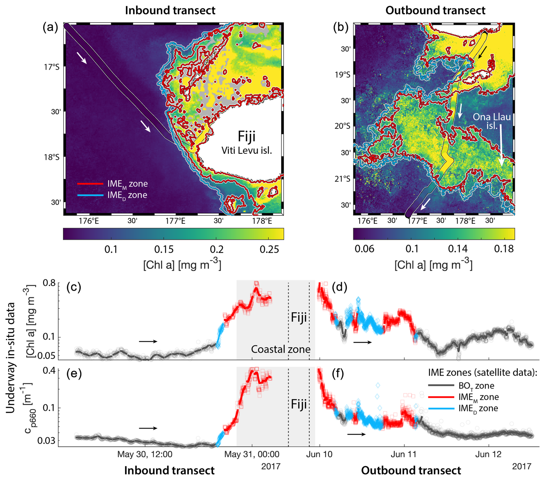
Figure 6 Validation of the extent of the IME using in situ underway data around the Fiji Archipelago. (a, b) The 8 d median [Chla] (a) at the time of sampling along the transect inbound to Fiji and (b) at the time of sampling along the transect outbound from Fiji. [Chla] measured in situ with the underway system is overlaid on the satellite data background. (c, d) Chlorophyll a concentration ([Chla]). (e, f) Beam attenuation at 660 nm (proxy for particulate organic carbon). Data sampled with the underway system during the transect (a, c, e) sailing towards Fiji and (b, d, f) sailing away from Fiji. Data colored when located within the IME zones detected on the overlapping 8 d satellite composite (BO_T, black circle; IME_M, red square; IME_D, blue diamond). The underway data points are minute-binned, and the solid lines are smoothed underway data. The smoothing was performed by applying a 2 h low-pass digital filter to the minute-binned data. The grey patch highlights the time Tara was sailing in coastal water (<6 nautical miles or 11 km away from a submerged reef or coast).

3.5 Extent of the IME using different algorithms

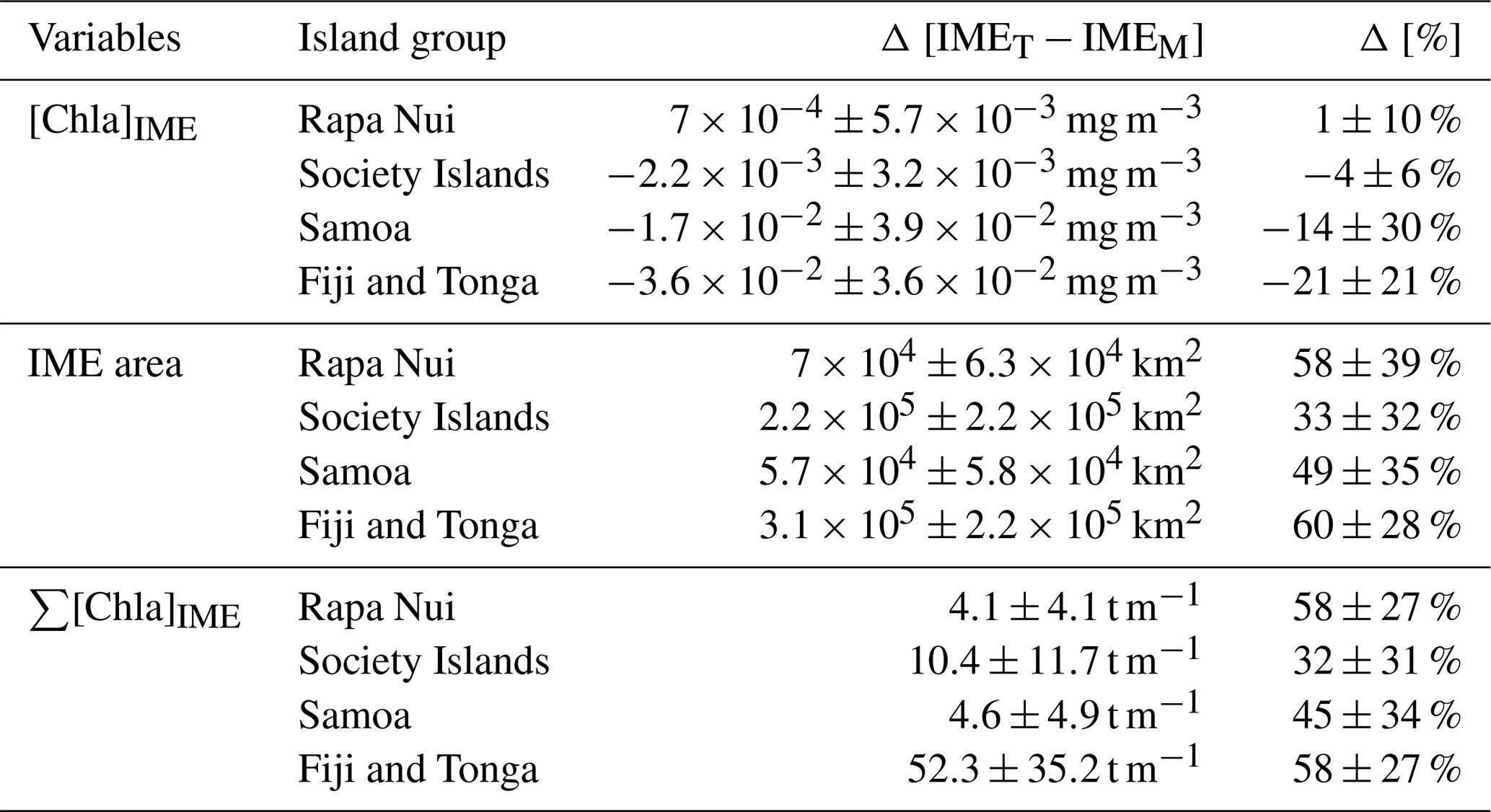
Similarly, the IME zones detected during the 6-month time series around Fiji–Tonga, Samoa–Niue, Rapa Nui, and the Society Islands (Figs. 2 and 3 and Bourdin, 2025) suggest that the IME_M detection algorithm generally performs well in capturing the core of an IME as long as the associated [Chla] distribution is concentric on the island with the highest [Chla] located close to shore. In all four case studies, the IME_M algorithm generally failed to capture the full extent of the IME area at 8 d observation frequency (i.e., IME_M area ≪ IME_T area; Fig. 7 and Table 2). To compare the IME_M algorithm to the one developed here, we calculated the absolute and percent differences in the mean [Chla], detected IME area, and surface-area-integrated chlorophyll a (∑[Chla]) derived from the two approaches applied on the same 8 d median [Chla] products (Fig. 7 and Table 2). [Chla] averages in IME_M zones were equivalent to or higher than those in the IME_T zones (Fig. 7 and Table 2) because the minimum value of the [Chla] used in the iteration to find the IME_T contour was always lower than the minimum value used in the IME_M algorithm. Therefore, when different from the IME_T contour, the IME_M contour was always located closer to the island shore where [Chla] is generally higher than in the rest of the IME_T zone, explaining the negative differences in average [Chla] between IME_T and IME_M (Table 2, Fig. 7). The area and surface-area-integrated chlorophyll a were largely underestimated in IME_M in comparison to IME_T in all four case studies (Fig. 7 and Table 2). For instance, the large bloom event that developed around Fiji between March and May 2017 detected in the IME_T zone was not detectable in the IME_M zone. IME_T also captured a nearly continuous increase in biomass around the Society Islands, while it was only intermittently captured by the IME_M contour (Fig. 7). In each case, the underestimation of IME_M compared to IME_T was variable over time, suggesting the criteria used to delineate the extent of IME_M are sensitive to noise in a given satellite image and thus depend on the spatial smoothness of the [Chla] map used to delineate IME_M. The modification of these criteria in the IME_T algorithm reduced its sensitivity to single-pixel variability.

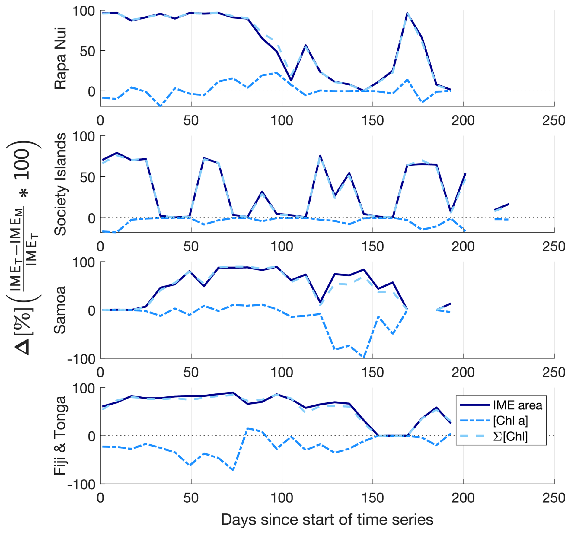
Figure 7 Differences (%) in the IME area (solid line), chlorophyll a concentration ([Chla]; dash-dotted line), and IME surface-area-integrated chlorophyll a (∑[Chla]_IME; dash line) estimated by the IME_M and IME_T algorithms for the four case studies (Rapa Nui, Society Islands, Samoa, Fiji–Tonga).

Table 2 IME_M and IME_T detection method comparison summary: 6-month mean and standard deviation of differences.

3.6 IME quantification metric

The [Chla] enhancement associated with the IME was quantified as the difference between surface-area-integrated [Chla] in a given IME zone and surface-area-integrated [Chla] in the respective BO zone (chosen to have the same surface area; see Method) to better represent the total Chla enhancement. In all four cases, the surface-area-integrated [Chla] enhancement associated with IME_T relative to their BO_T counterparts was significant during the entire 6-month time series (i.e., $\mathrm{\Delta }\sum [\mathrm{Chla}{]}_{{\mathrm{IME}}_{\mathrm{T}}-{\mathrm{BO}}_{\mathrm{T}}}-\mathrm{uncertainty}>\mathrm{0}$) except for two 8 d occurrences around Rapa Nui.

It should be emphasized that [Chla] can be associated with large uncertainties as a measure of phytoplankton biomass due to photoacclimation, a process of intracellular pigment adjustment in response to changes in light and nutrient conditions (Cullen, 1982; Geider et al., 1998). This is especially the case in regions with increased mesoscale activity and upwelling, such as those adjacent to islands. When low-light-adapted cells with larger intracellular [Chla] are upwelled to the surface, satellites can measure an apparent increase in [Chla] that is not necessarily associated with an increase in biomass (Hasegawa et al., 2008). In all case studies presented here, the increased [Chla] detected in IME zones was associated with increased c_p660, which is a proxy for total organic biomass (including phytoplankton biomass) that is not impacted by photoacclimation (Behrenfeld and Boss, 2006). This observation provides confidence that detected IME zones were indeed associated with spatial increases in phytoplankton biomass around islands. When investigating the ecological consequences of the IME, it is important to note that both satellite data and our underway measurements only describe surface ocean properties and do not provide information about the vertical distribution of biomass in IME zones. Gove et al. (2016) showed that the increase in [Chla] associated with the IME propagated below the surface and suggested this increase in [Chla] represented a strong increase in biomass at depth. Although strong subsurface chlorophyll maximums (SCMs) are generally measured in subtropical regions, most of the SCM signal is often due to photoacclimation from low light availability at depth and only associated with a moderate increase in biomass (Kitchen and Zaneveld, 1990; Fennel and Boss, 2003; Furuya, 1990).

3.7 The utility of capturing IME temporal dynamics

The high-temporal-resolution products revealed the high spatial and temporal heterogeneity of the IME and frequent connectivity between IME zones of distant islands. This dynamic IME detection method permitted tracking in time the accumulation of chlorophyll a standing stock in surface waters, which suggested frequent temporal increases in phytoplankton biomass in addition to the spatial increase in phytoplankton biomass already detected around islands. For instance, the accumulation of integrated [Chla] in IME zones suggests the occurrence of two distinct blooms in Samoa's IME zone and a large bloom in Fiji–Tonga's IME zone. These blooms were sustained for weeks while being advected offshore and eventually detached from the island they originated from (Figs. 2 and 3). The first one around Samoa was initiated around mid-September 2016 and was advected southward towards Niue (see area and $\mathrm{\Delta }[\mathrm{Chla}{]}_{{\mathrm{IME}}_{\mathrm{T}}-{\mathrm{BO}}_{\mathrm{T}}}$ increases; Fig. 5). The integrated [Chla] of this bloom continued to increase after the water mass detached from Samoa and persisted near Niue until the end of November 2016 (i.e., ∼ 10 weeks after detaching from Samoa; Figs. 3 and 5). The second bloom detected in Samoa's IME initiated around 22 November 2016 and was advected east, detaching from the archipelago and reaching a maximum surface-area-integrated [Chla] enhancement relative to a BO value of 13.6 t m⁻¹ before ending around 24 January 2017 (Figs. 3, 5). A third bloom observed in the same region detached from Tonga and was detected more than ∼ 1300 km east of the island. Phytoplankton biomass can continue to accumulate in advected water masses even without an additional influx of nutrients. For example, if the rate of horizontal dilution of a bloom with its surrounding oligotrophic waters reduces encounter rates and hence grazing pressure, phytoplankton biomass will continue to accumulate even if the remaining nutrients only support a low growth rate (as long as the growth rate exceeds the grazing rate; Lehahn et al., 2017). Interestingly, both bloom initiation events detected around Samoa were synchronized with a sudden increase in the average surface current velocity within the IME_M zone. The increased current interacting with the island topography may have promoted sub-mesoscale and mesoscale mixing and the upwelling of nutrient- and trace-metal-enriched water to the surface close to shore. The current data overlaid on the [Chla] map time series also show increased surface current close to the shore when and where each of the three blooms started to detach from their island of origin (Supplement Animation S1 and Bourdin, 2025). This suggests that when IME water parcels were detached from their source of nutrients (i.e., the island) and diluted into the surrounding oligotrophic ocean, the phytoplankton biomass in the growing patch continued to accumulate due to a reduction in grazing while using the limited nutrient supply advected with it. This dynamic emphasizes the fact that although phytoplankton blooms in IME zones are triggered by local enrichment of macronutrients and trace metals near islands (Messié et al., 2020, 2022; Gove et al., 2016, 2013; De Verneil et al., 2017; Hasegawa et al., 2009; Caputi et al., 2019; Palacios, 2002; Signorini et al., 1999), they are also tightly controlled by loss processes such as grazing. In the case of Fiji–Tonga, the IME surface-area-integrated [Chla] enhancement relative to the BO (i.e., $\mathrm{\Delta }\sum [\mathrm{Chla}{]}_{{\mathrm{IME}}_{\mathrm{T}}-{\mathrm{BO}}_{\mathrm{T}}}$) increased up to 88.7 ± 15.8 t_[Chla] m⁻¹ and covered an area up to $\sim \mathrm{1}\times {\mathrm{10}}^{\mathrm{6}}$ km², with a longitudinal extent of ∼ 2000 km. The IME surface-area-integrated [Chla] decreased from 5 May to 2 September to finally reach pre-bloom values again in August 2017, approximately 5 months after the bloom initiated (Fig. 4). In contrast to the Samoa case study, no apparent increase in current speed was detected near Fiji or Tonga during the period covered by the time series. In this case, the timing of this large bloom observed around the Fiji and Tonga archipelagos coincided with the annual Trichodesmium spp. blooms observed in this region during the austral summer (Dandonneau and Gohin, 1984; Dupouy et al., 2000). The high underwater volcanic activity characteristic of this region can supply a significant amount of trace metals directly into the euphotic zone and support these large blooms of Trichodesmium spp. (Bonnet et al., 2023; Guieu et al., 2018; Berman-Frank et al., 2001; Lory et al., 2022; Rubin et al., 2011). These known shallow hydrothermal vents were systematically located within the detected IME zone associated with Tonga and Fiji, suggesting the detected IME is likely a combined effect of islands and shallow hydrothermal vents in this region. The longer generation time of Trichodesmium spp., which allows surface currents to spread them horizontally, and their ability to partially escape grazing pressure may explain why these blooms can be maintained for 5 months and cover a significant area of $\sim \mathrm{1}\times {\mathrm{10}}^{\mathrm{6}}$ km² (Capone et al., 1997; Messié et al., 2020). These two case studies show how the dynamic detection of the IME provides information about IME phenology and about island connectivity in comparison to a frozen field observation of the ocean, for which all maps are independent of each other.

4 Conclusions

The method developed here describes the history of a given IME with finer resolution and highlights dynamics that are not detectable using monthly and yearly average remote sensing products. Such a method is essential for improving our mechanistic understanding of the IME (e.g., whether the cause is island runoff or upwelling) and the ecological succession within IMEs. De Falco et al. (2022) highlight the uniqueness of interactions between a given island topography and surrounding wind and current flows, suggesting that phytoplankton responses depend on these interactions. Here we show that IMEs are highly dynamic and that they can induce large coherent blooms that can sustain for months while being advected more than 1000 km away from their source. These advected IMEs seed the oligotrophic ocean and other islands with water masses characterized by higher phytoplankton abundance and potentially different species composition than the surrounding oligotrophic ocean, such as the Trichodesmium blooms in the southwestern Pacific Ocean. This analysis reveals a broader spatial extent of IMEs in subtropical regions, suggesting that islands have a greater impact on food web dynamics and biogeochemical processes in these areas, which are traditionally considered oligotrophic. This detection method can also be adapted to track water masses with specific optical properties being advected in upwelling regions or in river plumes. We suggest that future studies use more satellite variables than just [Chla] in regions where processes other than the one studied can cause elevated surface [Chla] to better discriminate the underlying processes.

We demonstrated the importance of using gapless high-temporal- and high-spatial-resolution satellite products and modeled surface currents to identify and track sub-mesoscale filaments and eddies associated with the IME around islands in the subtropical Pacific Ocean. We minimized satellite uncertainties by augmenting the number of observations and maximized data recovery using all available NASA and ESA polar-orbiting ocean color satellites. At the current dawn of global hyperspectral ocean color sensing, we recommend having sensors with different overpass times when planning for new ocean color satellites as part of the future constellation to help maximize coverage and understand the dynamics of mesoscale and sub-mesoscale processes in the ocean.

Appendix A: Satellite merging pipeline

MODIS, VIIRS, and OLCI L1A radiance data were processed with SeaDAS l2gen and POLYMER algorithms to produce atmospherically corrected level-2 R_rs data. Low-quality data pixels were removed by applying the recommended atmospheric correction flags to their respective R_rs data. Every scene was then projected onto the same equally spaced 1 km spatial resolution plate carrée reference grid using nearest-neighbor interpolation before [Chla] computation. Each satellite [Chla] was nudged to best match in situ values before merging them into 8 d median composites (Fig. A1).

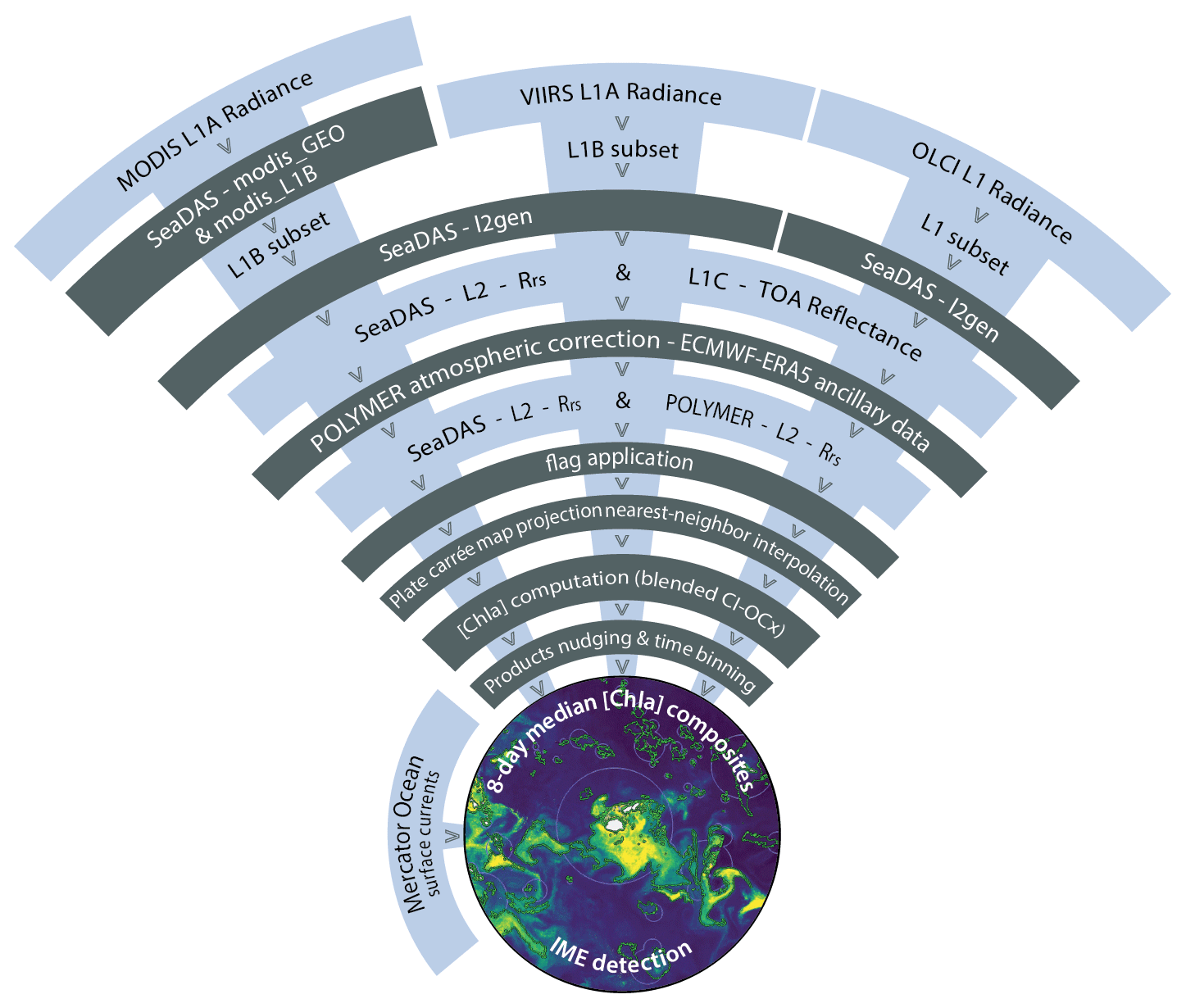
Figure A1 Satellite composite production flowchart.

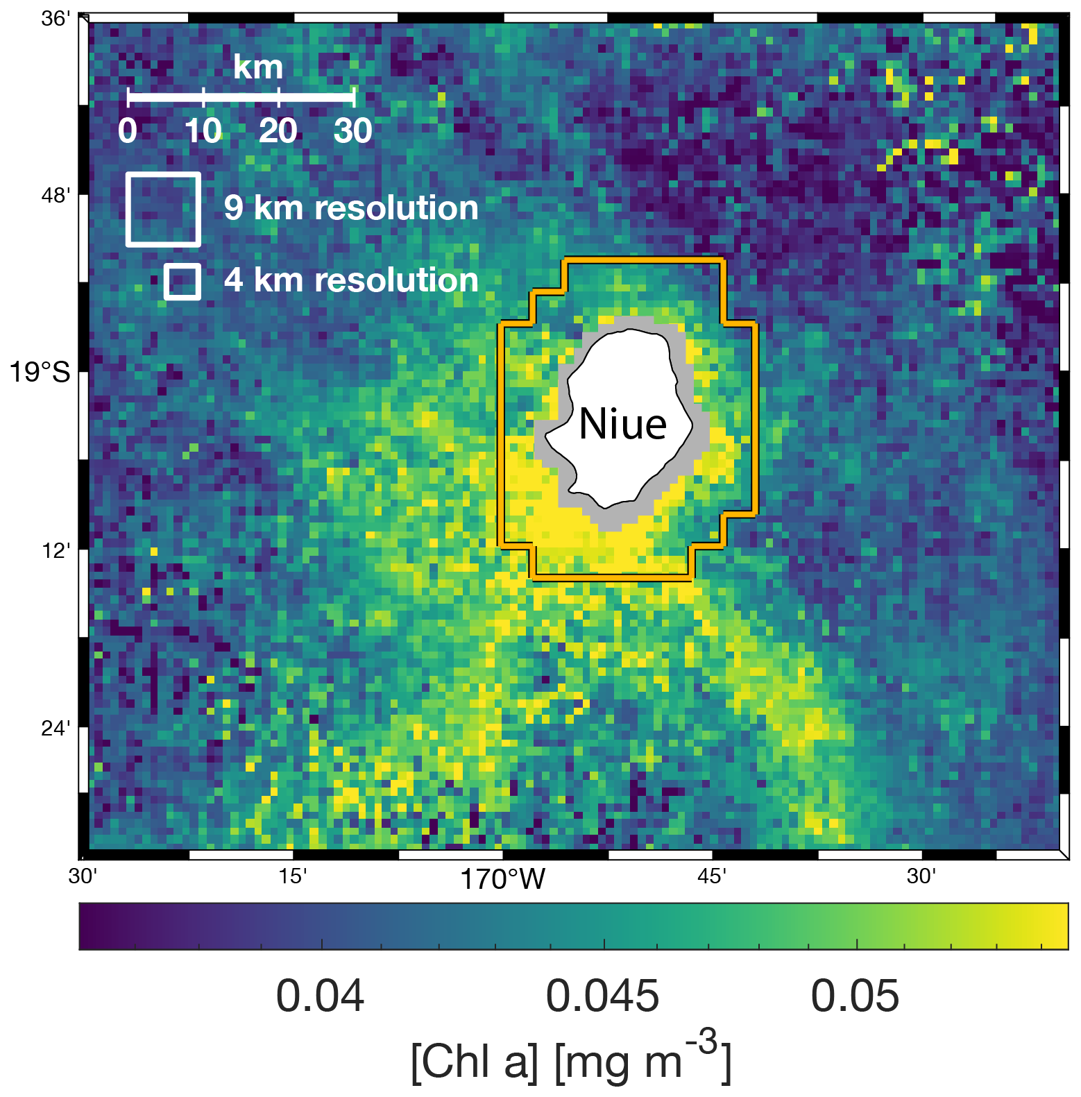
Figure A2 Multi-satellite composite of [Chla] around Niue (11 to 18 September 2016) at 1 km spatial resolution. The white squares represent the 4 and 9 km resolution pixel sizes of the level-3 NASA data, and the orange contour represents the shallow pixel mask at 4 km spatial resolution.

Appendix B: Uncertainty estimates

The 8 d merged products represent a composite of multiple overpasses and satellites that included ∼ 120 ocean color images (daytime) for a ∼ 2500 km² square region around the Fiji Archipelago. Therefore, each pixel of the merged product is a median of n observations of the original images with standard deviations (${\mathit{\sigma }}_{V_{\mathrm{bin}}}$) representing the temporal variability in a variable V in a given pixel during each 8 d period and the variability between sensors after nudging. The number of non-flagged observations ($n_{V_{\mathrm{bin}}}$) used to bin each merged pixel was generally sufficient, with 8 d long periods and an operational constellation of five to six satellites, to produce smooth merged [Chla] products. For example, the median number of non-flagged [Chla] observations used to bin each pixel was $n_{{\mathrm{bin}}_{\left[\mathrm{Chla}\right]}}=\mathrm{10}$ for the entire time series around Fiji, with less than 2.5 % of the pixels binned with less than 3 non-flagged observations (Fig. B1).

Known uncertainties were propagated from in situ data to satellite [Chla] end products. HPLC-derived [Chla] and in situ a_p spectra were measured in an along-track manner. The error associated with the computation of [Chla] from the underway system was estimated by the normalized root mean square error (nRMSE_udw in %) of the relation between the underway chlorophyll line height (a_p676LH) and total [Chla] measured from HPLC during the Tara Pacific Expedition (Fig. B2a).

The error associated with the computation of [Chla] from satellites was estimated by the nRMSE_sat of the relation between the underway chlorophyll line height (a_p676LH) and [Chla] obtained from each satellite sensor along the transect of the Tara Pacific Expedition (Fig. B2b, c, and d). The uncertainties in binned satellite end products were computed as follows:

$$\begin{array}{}\text{(B1)}& {\mathit{\sigma }}_{\mathrm{V}}=\sqrt{{\mathit{\sigma }}_{\mathrm{Vbin}}^{\mathrm{2}}+\sum _{n=\mathrm{1}}^{n_{\mathrm{c}}}(\stackrel{\mathrm{̃}}{V}\times {\mathrm{nRMSE}}_{\mathrm{c}}{)}^{\mathrm{2}}},\end{array}$$

where $\stackrel{\mathrm{̃}}{V}$ is the binned variable, n_c is the number of calibrations/corrections, and nRMSE_c is the nRMSE associated with each of the n_c corrections. The standard error in the mean of the adjusted satellite end products of each pixel was computed as follows:

$$\begin{array}{}\text{(B2)}& {\mathrm{SEM}}_{\mathrm{V}}={\displaystyle \frac{{\mathit{\sigma }}_{\mathrm{V}}}{\sqrt{n_{V_{\mathrm{bin}}}}}}.\end{array}$$

The final uncertainty estimate associated with [Chla] within entire IME or BO zones (${\mathrm{SEM}}_{[\mathrm{Chla}{]}_{\mathrm{IME}}}^{\mathrm{f}}$) as presented in Figs. E1, E2, 5, and 4 was expressed as the average standard error in the mean of the adjusted [Chla] within entire IME or BO zones:

$$\begin{array}{}\text{(B3)}& {\mathrm{SEM}}_{[\mathrm{Chla}{]}_{\mathrm{IME}}}^{\mathrm{f}}={\displaystyle \frac{{\stackrel{\mathrm{‾}}{\mathit{\sigma }}}_{[\mathrm{Chla}{]}_{\mathrm{IME}}}}{\sum n_{[\mathrm{Chla}{]}_{{\mathrm{bin}}_{\mathrm{IME}}}}}}+S_{[\mathrm{Chla}{]}_{\mathrm{unc}}}\times {\stackrel{\mathrm{‾}}{\left[\mathrm{Chla}\right]}}_{\mathrm{IME}},\end{array}$$

where $\sum n_{[\mathrm{Chla}{]}_{{\mathrm{bin}}_{\mathrm{IME}}}}$ is the total number of [Chla] observations within the IME zone before merging and $S_{[\mathrm{Chla}{]}_{\mathrm{unc}}}$ is the weighted bias associated with the computation of the slopes of the regressions between in situ [Chla] and each satellite [Chla] estimate. $S_{[\mathrm{Chla}{]}_{\mathrm{unc}}}$ was computed as follows:

$$\begin{array}{}\text{(B4)}& S_{[\mathrm{Chla}{]}_{\mathrm{unc}}}=|\mathrm{1}-S_{\left[\mathrm{Chla}\right]\mathrm{sat}}|\times {\displaystyle \frac{n_{M_{\mathrm{sat}}}}{N_{M_{\mathrm{tot}}}}},\end{array}$$

where S_[Chla]sat is the slope of the relation between in situ [Chla] and [Chla] of a given satellite, $n_{M_{\mathrm{sat}}}$ is the number of valid match-ups of the same satellite, and $N_{M_{\mathrm{tot}}}$ is the total number of valid match-ups. $S_{[\mathrm{Chla}{]}_{\mathrm{unc}}}$ represents the maximum bias associated with the computation of the merged satellite [Chla], which we assume to be equivalent to the potential likelihood bias of the merged satellite [Chla]. Assuming enough valid match-ups with each satellite, $S_{[\mathrm{Chla}{]}_{\mathrm{unc}}}$ is a conservative estimate of the bias associated with the slope computation because the merging method forces each satellite [Chla] to agree with in situ data using sensor-specific corrections, which likely reduces the bias of the merged product. IME area uncertainties (${\mathit{\sigma }}_{A_{\mathrm{IME}}}$) were computed during the detection of the IME [Chla] contours as the difference in the IME area between the last two iterations of [Chla] contours:

$$\begin{array}{}\text{(B5)}& {\mathit{\sigma }}_{A_{\mathrm{IME}}}=A_{{\mathrm{IME}}_{{\mathrm{cChl}}_{\mathrm{f}}}}-A_{{\mathrm{IME}}_{{\mathrm{cChl}}_{\mathrm{f}-\mathrm{1}}}},\end{array}$$

where $A_{{\mathrm{IME}}_{{\mathrm{cChl}}_{\mathrm{f}}}}$ is the IME area for the final IME contour value and $A_{{\mathrm{IME}}_{{\mathrm{cChl}}_{\mathrm{f}-\mathrm{1}}}}$ is the IME area for the previous contour value. Therefore, ${\mathit{\sigma }}_{A_{\mathrm{IME}}}$ represents the area detection resolution associated with the size of the step of the [Chla] iteration. The uncertainties associated with the estimation of IME surface-area-integrated [Chla] (∑[Chla]_IME) were computed as follows:

$$\begin{array}{}\text{(B6)}& \begin{array}{rl}{\mathrm{SEM}}_{\sum [\mathrm{Chla}{]}_{\mathrm{IME}}}^{\mathrm{f}}& =\sum [\mathrm{Chla}{]}_{\mathrm{IME}}\\ & \times \sqrt{{\left({\displaystyle \frac{{\mathrm{SEM}}_{[\mathrm{Chla}{]}_{\mathrm{IME}}}^{\mathrm{f}}}{{\stackrel{\mathrm{‾}}{\left[\mathrm{Chla}\right]}}_{\mathrm{IME}}}}\right)}^{\mathrm{2}}+{\left({\displaystyle \frac{{\mathit{\sigma }}_{A_{\mathrm{IME}}}}{A_{\mathrm{IME}}}}\right)}^{\mathrm{2}}}.\end{array}\end{array}$$

Figure B1 Distribution of the number of valid [Chla] (i.e., not flagged) observations per merged pixel over each 8 d period along the 6-month time series around the Fiji Archipelago (18 February to 5 September 2017).

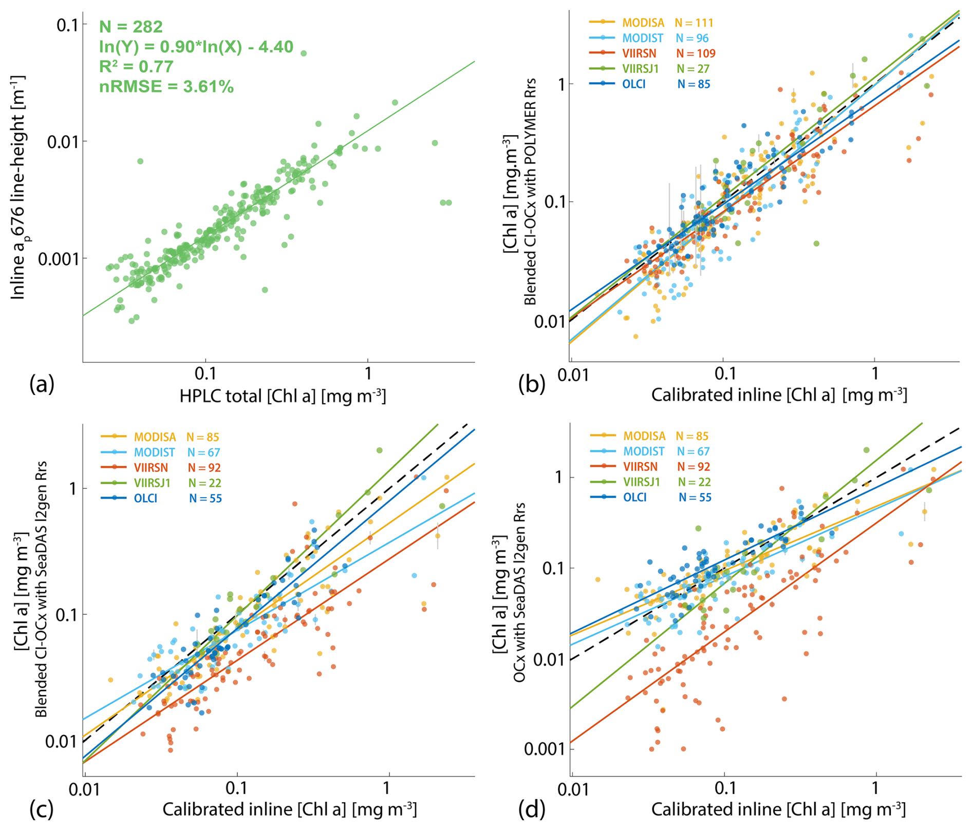
Figure B2 Robust linear regressions (a) between [Chla] measured from HPLC and the a_p [Chla] absorption peak at 676 nm measured from the underway system, (b) between calibrated [Chla] estimated from a_p underway measurements and [Chla] estimated from satellite data using the blended CI-OCx algorithm with POLYMER R_rs, (c) of the blended CI-OCx algorithm with l2gen R_rs, and (d) of the OCx algorithm with l2gen R_rs. In situ measurements were conducted during the Tara Pacific Expedition (May 2016 to October 2018).

Table B1 Robust correlations parameters of match-ups between satellite and in situ underway data.

Appendix C: Outlier removal

Bio-optical variables in the ocean, including [Chla], generally follow a log-normal distribution (Campbell, 1995) with fewer high values forming a heavy tail in the high end of the dynamic range. After appropriate flagging, low-quality data pixels impacted by sunglint, the adjacency effect, and bottom reflectance are rare and account for a few pixels scattered on either end of the log-normal distribution and beyond realistic values for a given region (generally < 1st percentile or ≫99th percentile; Fig. C1). Computing the median of these pixels can result in noisy merged products when they are the only available data over a given 8 d period and at a given location (i.e., pixel). Consequently, to improve the consistency of the level-3 merged products, rare outliers of a given variable were removed from all re-projected level-2 images of a given 8 d period and a given region based on the distribution of all individual x measurements (i.e., pixels). First, we grouped all the re-projected level-2 images of a given variable, 8 d period, and region together and applied a log-normal transformation to the data:

$$\begin{array}{}\text{(C1)}& x_t=\ln (x-min(x)+\mathrm{1}).\end{array}$$

We partitioned x_t into N bins of width W defined using the Freedman–Diaconis rule that is more suited to a heavy-tailed distribution due to its low sensitivity to outliers (Freedman and Diaconis, 1981):

$$\begin{array}{}\text{(C2)}& W=\mathrm{2}\times {\displaystyle \frac{\mathrm{IQR}\left(x_t\right)}{\sqrt[\mathrm{3}]{n}}},\end{array}$$

where IQR is the inter-quartile range and n is the number of observations in the data x_t. The minimum number of pixels per bin threshold ($n_{\min }^{\mathrm{b}}$) was computed as a rounded fraction of n of a given variable (i.e., horizontal line in Fig. C1):

$$\begin{array}{}\text{(C3)}& n_{\min }^{\mathrm{b}}=\lfloor n\times {\mathrm{10}}^{-\mathrm{6}}\rceil .\end{array}$$

The lower-end threshold t_L was determined by finding the first bin with fewer pixels than $n_{\min }^{\mathrm{b}}$ (i.e., gap in the normal distribution), going from the median $\stackrel{\mathrm{̃}}{x}$ to x_min ($x_{\min }\le t_{\mathrm{L}}<\stackrel{\mathrm{̃}}{x}$). Similarly, the higher-end threshold t_H was determined by finding the first bin with less than $n_{\min }^{\mathrm{b}}$ pixels per bin, going from $\stackrel{\mathrm{̃}}{x}$ to x_max ($\stackrel{\mathrm{̃}}{x}<t_{\mathrm{H}}\le x_{\max }$). This threshold detection was iterated up to 15 times or until t_L and t_H did not change from one iteration to the other. Any re-projected level-2 pixel from a given 8 d period, region, and variable falling out of the range (t_L, t_H) was deleted before computing the medians of the merged level-3 products.

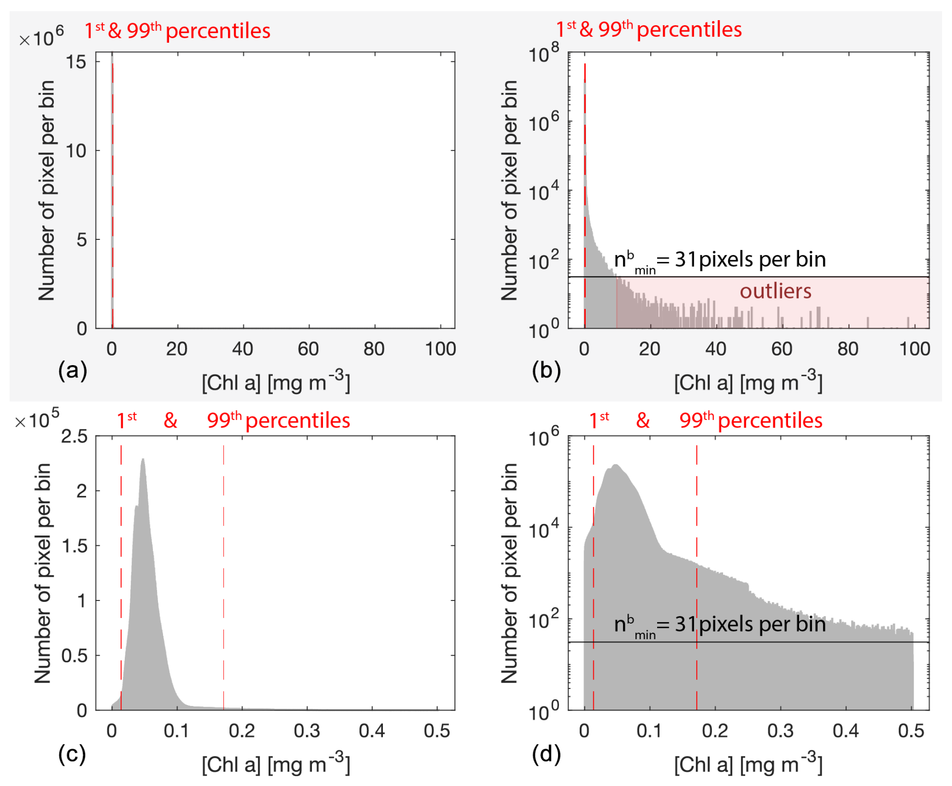
Figure C1 Example distribution of all valid [Chla] (i.e., not flagged) observations from all satellite sensors merged (i.e., MODIS Aqua, MODIS Terra, VIIRS SNPP, OLCI S3A) from 19 September 2016 at 01:00 to 26 September 2016 at 21:30 UTC (8 d period) around Niue and Samoa (77 satellite images merged) before outlier removal (panels a and b) and after outlier removal (panels c and d). The number of pixels per bin is displayed on a linear scale in panels (a) and (c) and on a log base-10 scale in panels (b) and (d). The dashed lines represent the 1st and the 99th percentiles, the solid horizontal line represents the cut-off value in pixels per bin for outlier removal ($n_{\min }^{\mathrm{b}}$), and the red-shaded area highlights the pixels removed.

Appendix D: Rapa Nui, Society Islands, and Samoa validation transects

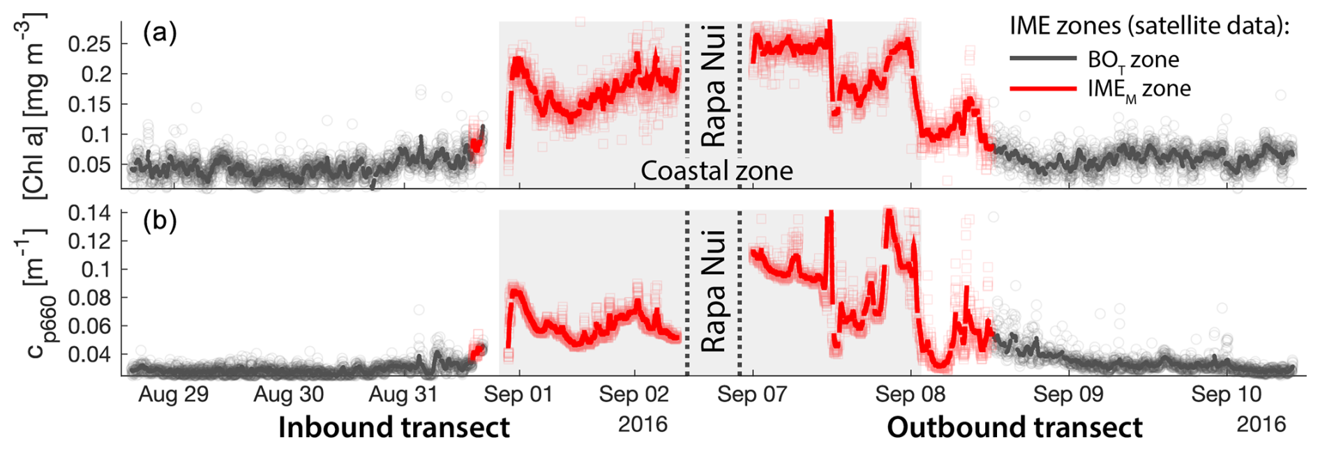
Figure D1 Validation of the IME extent using in situ underway data around Rapa Nui. (a) Chlorophyll a concentration ([Chla]) and (b) beam attenuation at 660 nm (proxy for particulate organic carbon). Data sampled with the underway system during the transect sailing towards Rapa Nui (left) and sailing away from Rapa Nui (right). Data colored when located within the IME zones detected in the overlapping 8 d satellite composite (BO_T, black circle; IME_M, red square). The points are minute-binned underway data, and the solid lines are smoothed underway data. The smoothing was performed by applying a 2 h low-pass digital filter to the minute-binned data. The grey patch highlights the time Tara was sailing in coastal water (<50 m depth).

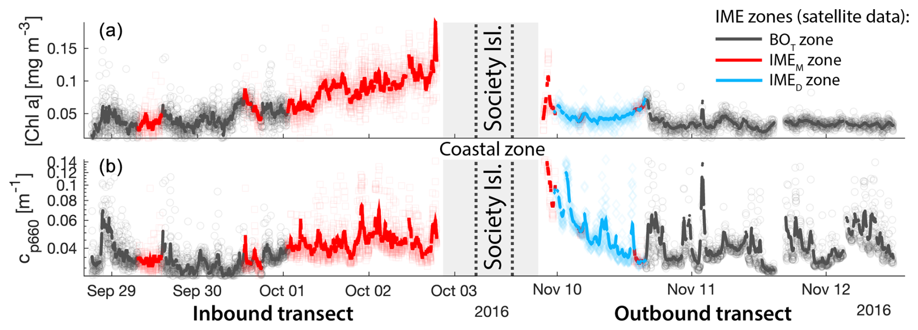
Figure D2 Validation of the IME extent using in situ underway data around the Society Islands in French Polynesia. (a) Chlorophyll a concentration ([Chla]) and (b) beam attenuation at 660 nm (proxy for particulate organic carbon). Data sampled with the underway system during the transect sailing towards the Society Islands (left) and sailing away from the Society Islands (right). Data colored when located within the IME zones detected in the overlapping 8 d satellite composite (BO_T, black circle; IME_M, red square; IME_D, blue diamond). The points are minute-binned underway data, and the solid lines are smoothed underway data. The smoothing was performed by applying a 2 h low-pass digital filter to the minute-binned data. The grey patch highlights the time Tara was sailing in coastal water (<50 m depth).

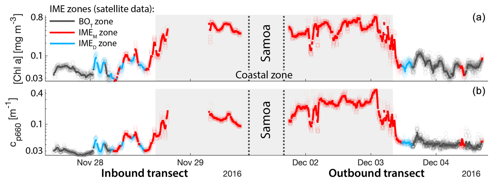
Figure D3 Validation of the IME extent using in situ underway data around Samoa. (a) Chlorophyll a concentration ([Chla]) and (b) beam attenuation at 660 nm (proxy for particulate organic carbon). Data sampled with the underway system during the transect sailing towards Samoa (left) and sailing away from Samoa (right). Data colored when located within the IME zones detected in the overlapping 8 d satellite composite (BO_T, black circle; IME_M, red square; IME_D, blue diamond). The points are minute-binned underway data, and the solid lines are smoothed underway data. The smoothing was performed by applying a 2 h low-pass digital filter to the minute-binned data. The grey patch highlights the time Tara was sailing in coastal water (<50 m depth).

Appendix E: Rapa Nui and Society Islands time series

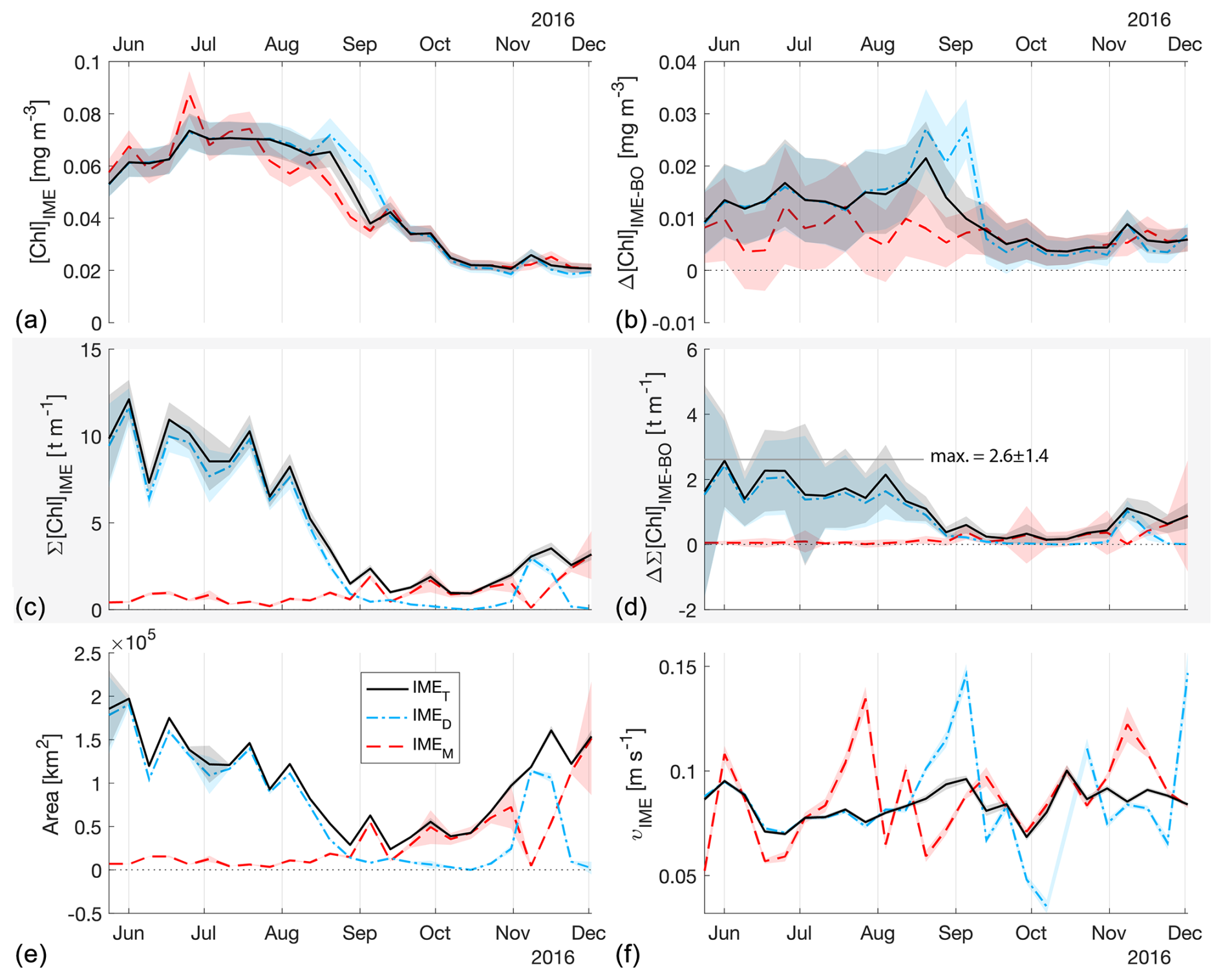
Figure E1 The 6-month-long time series of satellite-derived IME properties of the IME zones (IME_M, dashed red line; IME_D, dash-dotted blue line; IME_T, solid black line) detected around Rapa Nui. (a) Average chlorophyll a concentration within the IME zones ([Chla]_IME), (b) difference in average [Chla] values between each IME zone and their respective BO zones (Δ[Chla]_IME−BO), (c) IME surface-area-integrated chlorophyll a (∑[Chla]_IME), (d) difference in IME and BO surface-area-integrated chlorophyll a ($\mathrm{\Delta }\sum [\mathrm{Chla}{]}_{\mathrm{IME}-\mathrm{BO}}$), (e) IME zone area, and (f) surface current velocity.

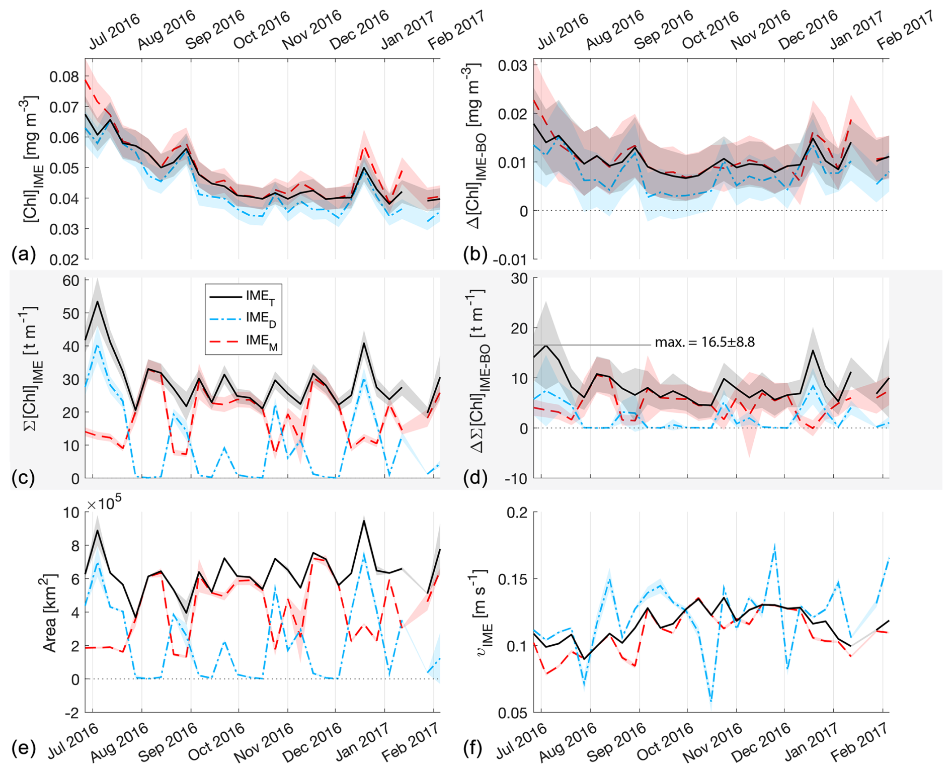
Figure E2 The 6-month-long time series of satellite-derived IME properties of the IME zones (IME_M, dashed red line; IME_D, dash-dotted blue line; IME_T, solid black line) detected around the Society Islands in French Polynesia. (a) Average chlorophyll a concentration within the IME zones ([Chla]_IME), (b) difference in average [Chla] values between each IME zone and their respective BO zones (Δ[Chla]_IME−BO), (c) IME surface-area-integrated chlorophyll a (∑[Chla]_IME), (d) difference in IME and BO surface-area-integrated chlorophyll a ($\mathrm{\Delta }\sum [\mathrm{Chla}{]}_{\mathrm{IME}-\mathrm{BO}}$), (e) IME zone area, and (f) surface current velocity.