Improved understanding of nitrate trends, eutrophication indicators, and risk areas using machine learning

Nitrate is an essential inorganic nutrient limiting phytoplankton growth in many marine environments. Eutrophication, often caused by nitrogen deposition, is a reoccurring problem in coastal regions, including the North-West European Shelf (NWES). Despite their importance, nitrate observations on the NWES are costly to obtain and thus sparse in both time and space. We demonstrate that machine learning (ML) can generate, from sparse observations, a skilled, gap-free, bi-decadal (1998–2020) surface nitrate dataset. We demonstrate that the effective resolution (scales on which the dataset is skilled) is slightly coarser than the 7 km and daily resolution of the product but still completely sufficient to analyse nitrate dynamics on a monthly scale. With such a dataset we are able to (i) highlight the coastal regions that show strong summer nutrient limitation, covering eutrophication problem areas identified by monitoring bodies (i.e. OSPAR), but also other regions, such as the southern Irish coastline and parts of the Irish Sea. Our results could indicate greater potential for eutrophication events in regions subject to high-riverine-nutrient-discharge scenarios. (ii) We demonstrate that bi-decadal 1998–2020 trends in coastal nitrate, responding to long-term policy-driven reduction in riverine discharge, are mostly modest, with a notable exception of the Bay of Biscay. (iii) We show that winter nitrate plays a relatively minor direct role in the intensity of the phytoplankton bloom the following spring, which can have some implications for using winter inorganic nitrogen as an indicator of eutrophication (as often included by OSPAR). The last two results are consistent with recent findings in the literature (Axe et al., 2022; Devlin et al., 2023; Van Leeuwen et al., 2023). We propose using the nitrate dataset for data assimilation and hypothesise that it has the potential to substantially improve phytoplankton forecasts in operational runs.

1 Introduction

Nitrogen is one of the most important components of organic matter, needed for primary production in relatively large concentrations, as demonstrated by the Redfield ratios (Tett et al., 1985). Despite its large abundance (the Earth's atmosphere comprises 78 % of nitrogen as N₂), it is non-trivial to obtain nitrogen in forms useful for plants. As a consequence, nitrogen is often the most limiting nutrient for plant or algae growth, including the coastal marine environment (Ryther and Dunstan, 1971; Board and Council, 2000). Nitrogen fixation, converting atmospheric nitrogen to forms useful for life, happens through various biotic and abiotic pathways, resulting in ammonium, nitrite, and nitrate (Noxon, 1976; Hill et al., 1980; Postgate, 1998; Beman et al., 2008; Voss et al., 2013). Nitrate in the ocean is the primary nutrient for phytoplankton, with phytoplankton uptake enabling nitrogen flows into higher trophic levels and various detrital and dissolved forms of organic matter. In a nitrogen-limited environment, excess nitrate concentrations, primarily originating from agricultural runoff and industrial wastewater discharge, can stimulate harmful eutrophication events (Withers et al., 2014; Nazari-Sharabian et al., 2018). The thick layer of algae produced by these events may reduce oxygen ventilation at the surface, and after the algae die off and sink, decomposers may consume vast amounts of oxygen, leading to marine hypoxia in the bottom part of the water column (Rabalais et al., 2002; Diaz and Rosenberg, 2008). Furthermore, eutrophication events are often dominated by species that produce toxins (leading to harmful algae blooms, HABs), which have detrimental effects on the marine ecosystem by causing fish kills, contaminating seafood, and even posing risks to human lives (Anderson et al., 2012). Additionally, high nitrate concentrations may lead to excessive production of organic matter under certain circumstances, which, upon decomposition, increases CO₂ concentrations, contributing to ocean acidification (Doney et al., 2009). Eutrophication is a fundamental problem in many shelf sea and coastal areas (Rabalais et al., 2009), where nitrate monitoring and prediction, along with other indicators (e.g. chlorophyll, dissolved oxygen, phytoplankton species), provide an essential tool informing marine management and policy.

An important region subject to eutrophication is the North-West European Shelf (NWES). The NWES is impacted by significant river inputs, such as the Elbe, Rhine, Loire, Seine, Scheldt, Meuse, Humber, Weser, and Thames, which introduce substantial freshwater and nutrients into the region, influencing salinity and water properties (Sonesten et al., 2022). Open ocean–shelf exchange, especially transport of nutrients and carbon across the shelf break, plays another vital role in the NWES ecosystem dynamics (Huthnance et al., 2009). The NWES has high ecological importance due to its high biological productivity, underpinning significant commercial fisheries and carbon sequestration (Pauly et al., 2002; Borges et al., 2006; Jahnke, 2010). Until the 1980s, the NWES, particularly near the German Bight and the Westerschelde Estuary, experienced notable shifts in nutrient distribution, primarily driven by increased continental nutrient inputs. Riverine discharges, particularly from the Rhine and Elbe, have been identified as major contributors to nutrient dynamics in the region (Brockmann and Eberlein, 1986; Radach, 1992), having adverse effects on the local ecosystem. However, EU regulations following the OSPAR Convention in 1992 have substantially decreased nitrate deposition into the NWES (Soetaert et al., 2006; Radach and Pätsch, 2007; Lenhart and Große, 2018; Burson et al., 2016; Axe et al., 2022; Sonesten et al., 2022).

The NWES nitrate concentrations are operationally simulated and predicted (Skákala et al., 2018); however, NWES nitrate observations are too sparse to properly constrain the simulated nitrate through data assimilation. Existing works have developed statistical algorithms to derive nitrate from satellite observations (Durairaj et al., 2015; Chen et al., 2023), but these have so far been developed either for the global open ocean or for regions other than the NWES (such as different regions in Asia or California, Yu et al., 2021; Chen et al., 2023), and those algorithms are unlikely to work for the NWES. The current operational NWES system is mainly constrained by much more robust satellite temperature and chlorophyll observations (Skákala et al., 2018, 2021, 2022) and avoids assimilating nutrients entirely. Furthermore, due to its univariate nature, the operational system fails to directly constrain most of the non-assimilated variables, including nutrients. Consequently, the nitrate reanalyses and forecasts produced by the operational system are known to have substantial biases, inherited from the model free run (Skákala et al., 2018, 2022). Although the simulated physics and chlorophyll from the reanalysis are well validated against observations (Skákala et al., 2018, 2022), the nitrate NWES product is of more limited use.

In this work we develop and validate a new bi-decadal NWES nitrate product derived from available observations using advanced machine learning (ML) algorithms. The nitrate product is developed for the ocean surface, where nutrients have the potential to most significantly drive phytoplankton growth. This is, to our knowledge, by far the most complete and detailed observation-based sea surface nitrate dataset on the NWES. Unlike the NWES operational reanalysis, the dataset validates skilfully against the independent observations. Using our NWES nitrate product, we are able to discuss several important topics, like the impact of winter nitrate pre-conditioning on interannual phytoplankton variability, the most nutrient-limited coastal NWES geographic areas, and the trends in nitrate concentrations on the NWES. To do so, we maximise our reliance on the observational data and use ML and modelling to effectively fill the large data gaps, either through statistics or through dynamical consistency imposed by deterministic modelling.

2 Methodology

2.1 The ML model

We used as the ML model a feed-forward neural network (NN) designed through the Autokeras library using a structured data regressor (Jin et al., 2019). This approach streamlined the process of hyperparameter optimisation and model architecture discovery through an automated procedure, significantly reducing the need for manual intervention. The routine follows an iterative trial-and-error approach by looping through several possible combinations of various hyperparameters, such as learning rate, optimisers, and the number of dense layers with different combinations of nodes. It then selects the best model architecture with the highest skill score against the validation dataset and saves it for final prediction against the test data.

The final model architecture comprised several layers (see Fig. S1 in the Supplement): (i) the input layer, with 25 nodes, corresponds to the input features or predictors; (ii) a multi-category encoding layer, encoding categorical features (i.e. month and day of the year) into a numeric form that can be understood by the network; (iii) a normalisation layer, which normalises the input data to improve model training by facilitating improved model convergence time and better performance, avoiding dominance of features with larger magnitudes, and providing better stability; (iv) two dense layers with 128 and 256 nodes, respectively, with each of these layers being followed by a rectified linear unit (ReLU) activation function to introduce non-linearity into the model; (v) a dropout layer that is applied to prevent overfitting by randomly dropping out a fraction of neurons during the training phase; and (vi) a regression head with a single node that produces the final prediction, i.e. nutrient concentration. During the training phase, the model's performance was evaluated using standard metrics, i.e. mean squared error (MSE), and the relative error was then estimated with respect to the validation dataset.

2.2 Data

2.2.1 The input features

To avoid biases towards operational models, the NN model input features were selected to be either observational data or reanalyses of variables closely constrained by the observations. One of the main challenges in developing ML for environmental applications is combining (often sparse) data with typically inconsistent domains of coverage across various spatial and temporal scales. The most robust NWES-focused observational datasets are obtained through satellite optical measurements. For physics, these are data such as sea surface temperature (SST) or altimetry. For biogeochemistry, the most typically derived dataset is surface chlorophyll a concentration obtained from the ocean colour (OC). Recently, new remote-sensing algorithms have been developed to partition the total chlorophyll concentration into phytoplankton functional types (PFTs) largely based on phytoplankton size classes (Brewin et al., 2010, 2017), and PFT chlorophyll products are now operationally assimilated into the NWES model (Skákala et al., 2018). The reanalyses from the NWES operational model have been found to have very close match-ups with the assimilated observations (Skákala et al., 2018, 2022) and act as natural extensions of the observations, forming a complete dataset on a gridded domain. We have extracted a range of NN model features from NWES physical–biogeochemistry reanalysis products, namely NWSHELF_MULTIYEAR_BGC_004_011 and NWSHELF_MULTIYEAR-_PHY-_004_009 (downloadable from the EU Copernicus portal, https://data.marine.copernicus.eu/product/NWSHELF_MULTIYEAR_BGC_004_011/services, last access: 20 June 2025; see also Kay et al., 2016), covering the 1998–2020 period with daily and 7 km spatial resolution. The product is based on assimilating satellite SST, temperature, and salinity profiles, as well as OC PFT chlorophyll, into the operational Nucleus for European Modelling of the Ocean (NEMO; Madec et al., 2017) model coupled through the Framework for Aquatic Biogeochemical Models (FABM; Bruggeman and Bolding, 2014) to the biogeochemistry European Regional Seas Ecosystem Model (ERSEM; Baretta et al., 1995; Butenschön et al., 2016). The extracted features were for (i) SST; (ii) chlorophyll ocean surface concentrations from four PFTs, which were assimilated into NEMO-FABM-ERSEM (diatoms, microphytoplankton, nanophytoplankton, and picophytoplankton); (iii) total surface phytoplankton carbon; (iv) total surface chlorophyll; and (v) total surface net primary production. Although these features were selected from the reanalysis, they correspond to either the assimilated variables (SST, PFT chlorophyll) or the variables which are dynamically very close to the assimilated PFT chlorophyll (phytoplankton carbon, net primary production) and therefore well constrained by the assimilation. Additionally, we also included SST observations from the global ocean OSTIA product (Good et al., 2020; Donlon et al., 2012) in the input feature dataset. Interestingly, our tests (not shown here) indicated that the NN model did not perform as well without this additional SST dataset, so both sources of SST information (reanalysis and OSTIA) were used.

We have also used input features describing riverine discharge into the ocean. These included riverine discharge data for oxygen and nutrient loads (i.e. nitrate, phosphate, silicate, ammonia, and oxygen) at all relevant river mouths in the NWES domain. Daily time series of river discharge are used for 1998–2017. From 2018, only climatologies were available and were used for the remaining 2018–2020 period. The daily riverine data were obtained from an updated version of the river dataset from Lenhart et al. (2010). The climatology of daily discharge data was taken from the Global River Discharge Database and the Centre for Ecology & Hydrology (Young and Holt, 2007). Unlike a hydrodynamic model, an NN model does not follow any advection mechanism or transport to carry the effect of river discharge over space and time. To account for advection, the NN model would have to ideally include time-lagged riverine inputs, where the time lag would increase with the spatial distance from the river mouth. This would hugely increase the complexity of the NN model. In this work we have decided to opt for less complex models and avoid using time-lagged NN inputs. To consider a nearly instantaneous riverine effect in a simplified way, we have distributed the riverine discharge data around the river discharge point sources. This was done by spatially extrapolating all the runoff variables at all the daily discharge points over a 50 km circular radius surrounding the main discharge point, by making the inputs decay inversely from the maximum at the centre to a zero value at the edge (see Fig. 1). However, such a scheme is clearly a major simplification of the real river impact (e.g. Painting et al., 2013; Lenhart and Große, 2018) and should ideally be improved upon in future work.

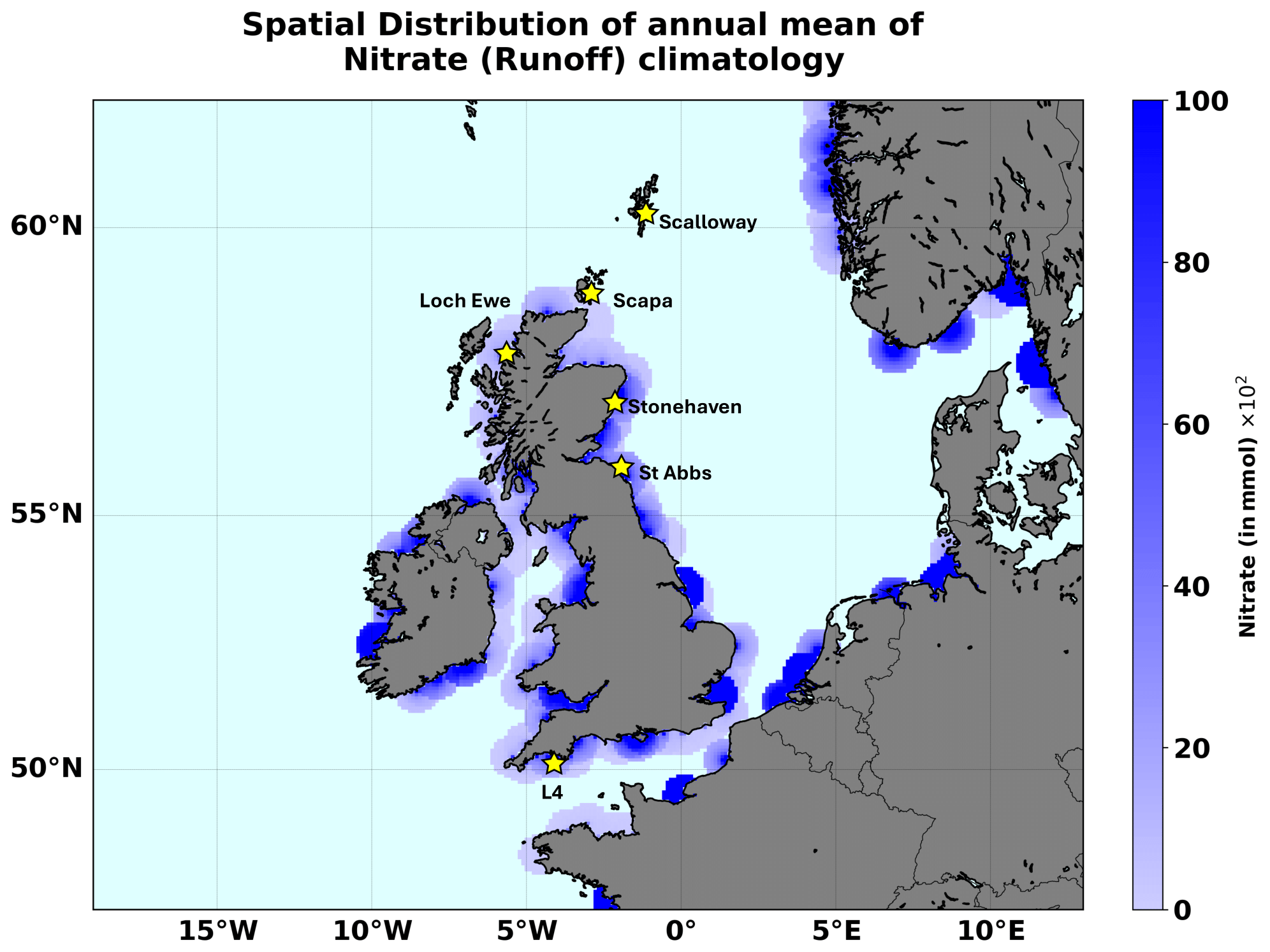
Figure 1 The areas with river input on the NWES domain. We mark the locations of the stations providing the test data for this study: L4 and the five Scottish coastal stations.

Another dataset that was used as input features into the NN model was the ERA5 atmospheric reanalysis (Hersbach et al., 2020), which has a horizontal resolution of 0.25°. The input feature dataset includes variables such as downwelling shortwave radiation at the ocean surface, specific humidity, temperature at 2 m above the ocean surface, sea level pressure, total precipitation, and zonal and meridional wind components at 10 m above the ocean surface. These near-surface atmospheric drivers play a crucial role in governing and redistributing surface nitrate through air–sea interactions and atmospheric deposition of nitrogen, which accounts for one-third of the non-recycled nitrogen supply in the ocean and up to around 3 % of annual new biological production (Arrigo et al., 2008). The atmospheric data, however, did not include any direct products for atmospheric nitrogen deposition. Finally, we used structural temporal and geographic data, i.e. the time of the year (month, day), latitude, longitude, depth, and bathymetry, as input features. This type of information enables the model to learn the geographic patterns in nitrate, including its seasonal climatology, substantially enhancing its predictive accuracy.

All the input features were considered at the same time as the predicted nitrate. The input features' importance was ranked in the SHapley Additive exPlanations (SHAP) analysis, presented in Fig. S2 in the Supplement. The SHAP analysis indicates that the structural input features are among the most important, followed by some atmospheric and oceanic physics features (incoming shortwave radiation, SST), which can partly account for seasonal climatology as well. Specific riverine discharge input features (e.g. of nitrate itself) are highly important too (Fig. S2), with a range of biogeochemical variables (total surface chlorophyll, total surface net primary production, and total surface carbon) being around the middle of the importance ranking. As already mentioned, we also tested versions of the NN model with a reduced number of input features (e.g. removing the less important features from the SHAP analysis), but the model's performance became slightly worse compared to that of the previous model.

2.2.2 The predicted nitrate data and the training and validation process

The 1998–2018 nitrate observations were obtained from the International Council for the Exploration of the Sea (ICES) data portal (https://www.ices.dk, last access: 20 June 2025). The extracted dataset spans a geographical range from 19° W to 10° E in longitude and 47 to 62° N in latitude, ensuring a broad representation of the dynamics and variability of the NWES region. The ICES data were obtained from a wide range of in situ measurements, e.g. by cruises, floats, moorings, and buoys. In the training and validation process, the ML model inputs were linearly interpolated onto the ICES data locations, and then the ICES data from the 1998–2015 period, containing 43 572 relevant data points, were used for training and validation of the NN model (with 80 % of data used for training and 20 % for validation). Finally, the 2016–2018 ICES data, containing 2984 data points, were used as test data. The spatial coverage of all the ICES training, validation, and test data is shown in Fig. 2.

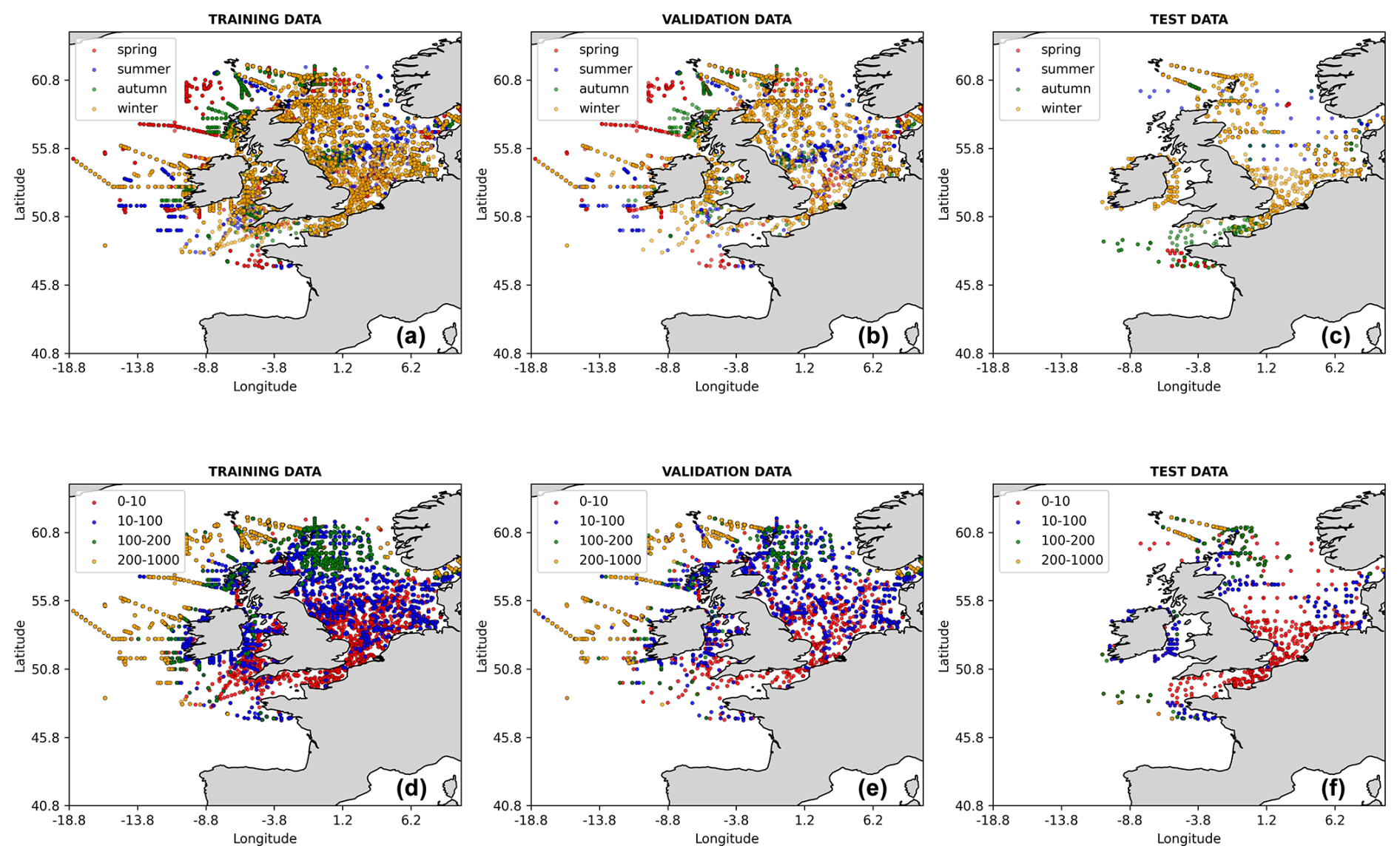
Figure 2 The locations of the ICES data used in this study, split into training, validation, and test data. The data points are coloured with respect to the season in which the measurement was taken (a–c) and the depth range (in m) at which the measurement was taken (d–f).

Several other observations were used as test data to demonstrate the ML model's skill: (i) nitrate data from the L4 station, which is operated by the Western Channel Observatory (https://www.westernchannelobservatory.org.uk/data.php, last access: 20 June 2025) and is located in the western English Channel approximately 13 km from the Plymouth Sound, providing one of the longest continuous ecological time series in the world (Harris, 2010). The L4 nitrate dataset covered the whole 1998–2020 period, and despite several data gaps, during most of this period it was sampled with a frequency of approximately 5–7 d. (ii) Another independent nitrate test dataset was obtained from the Scottish Coastal Observatory Dataset (https://data.marine.gov.scot/dataset/scottish-coastal-observatory-dataset-1997-2020, last access: 20 June 2025; see also Bresnan et al., 2016; Hindson et al., 2018), covering five locations near the coastline of Scotland (Loch Ewe, Scalloway, Scapa, St Abbs, Stonehaven) and providing time series of differing lengths: from the longest, covering the 2008–2020 period (Scapa, Scalloway), to the shortest, covering the 2017–2020 period (St Abbs). The measurements at these stations typically had a frequency of 5–7 d. The locations of the L4 station and the five Scottish stations are all marked in Fig. 1. It should be noted that neither the L4 data nor the data from the Scottish stations were included in the ICES dataset.

Finally, after validating the NN model, we ran it for the full 1998–2020 period across the whole Copernicus NWES reanalysis domain (see Fig. 3), using Copernicus reanalysis, river input, and ERA5 atmospheric forcing input (with both inputs interpolated onto the Copernicus reanalysis domain) to produce a gap-free, bi-decadal, daily 7 km resolution reconstruction of nitrate. This final dataset underpins the results from this study.

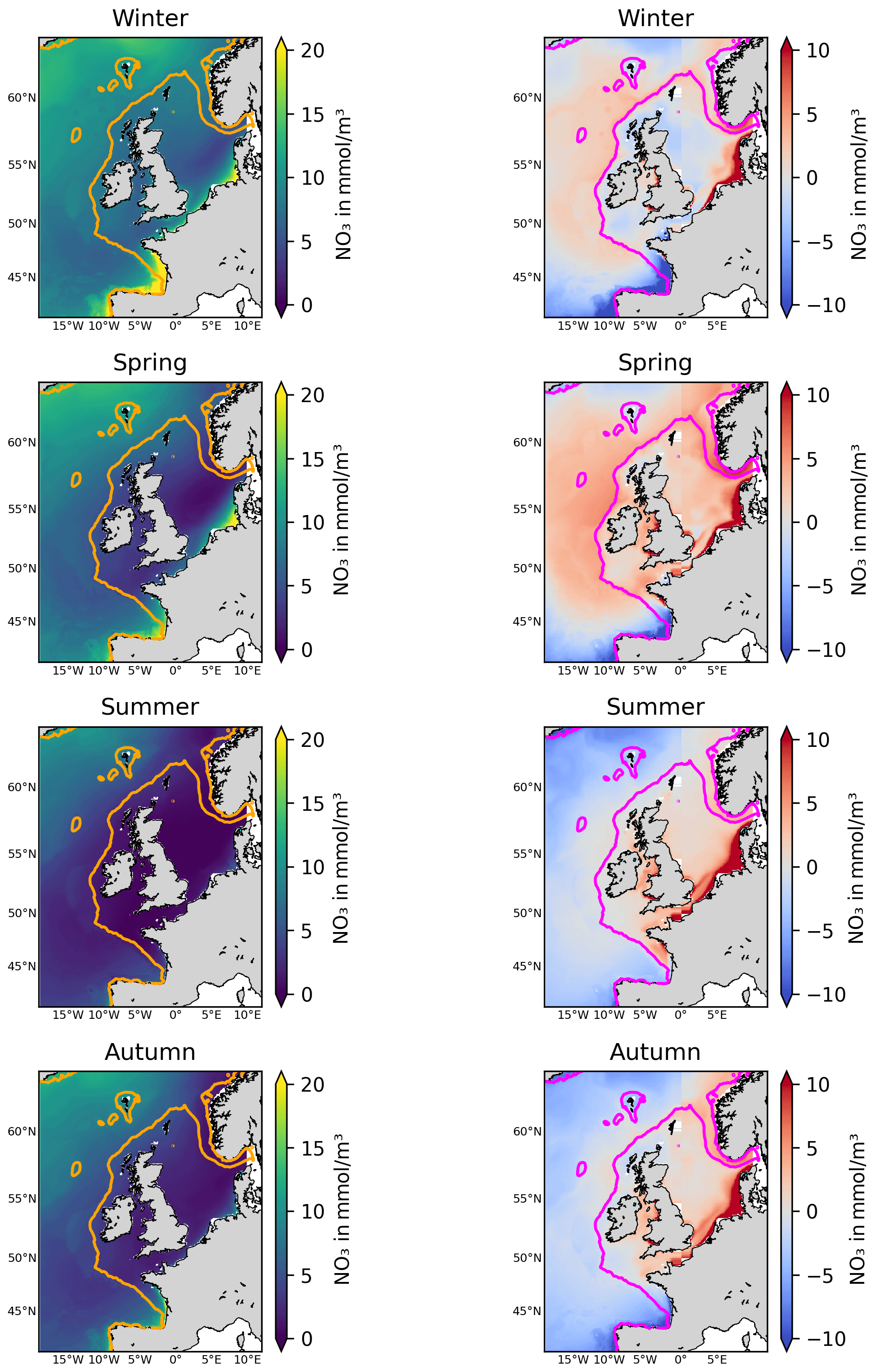
Figure 3 The left-hand panels show the NN-reconstructed 1998–2020 average surface nitrate concentrations for different seasons (corresponding to the dominant mode of temporal variability in nitrate). The right-hand panels show the same averages for the relative bias of the Copernicus surface nitrate reanalysis (Kay et al., 2016) with respect to the NN-reconstructed dataset (reanalysis minus NN-reconstructed dataset). The contours mark the NWES (bathymetry <200 m).

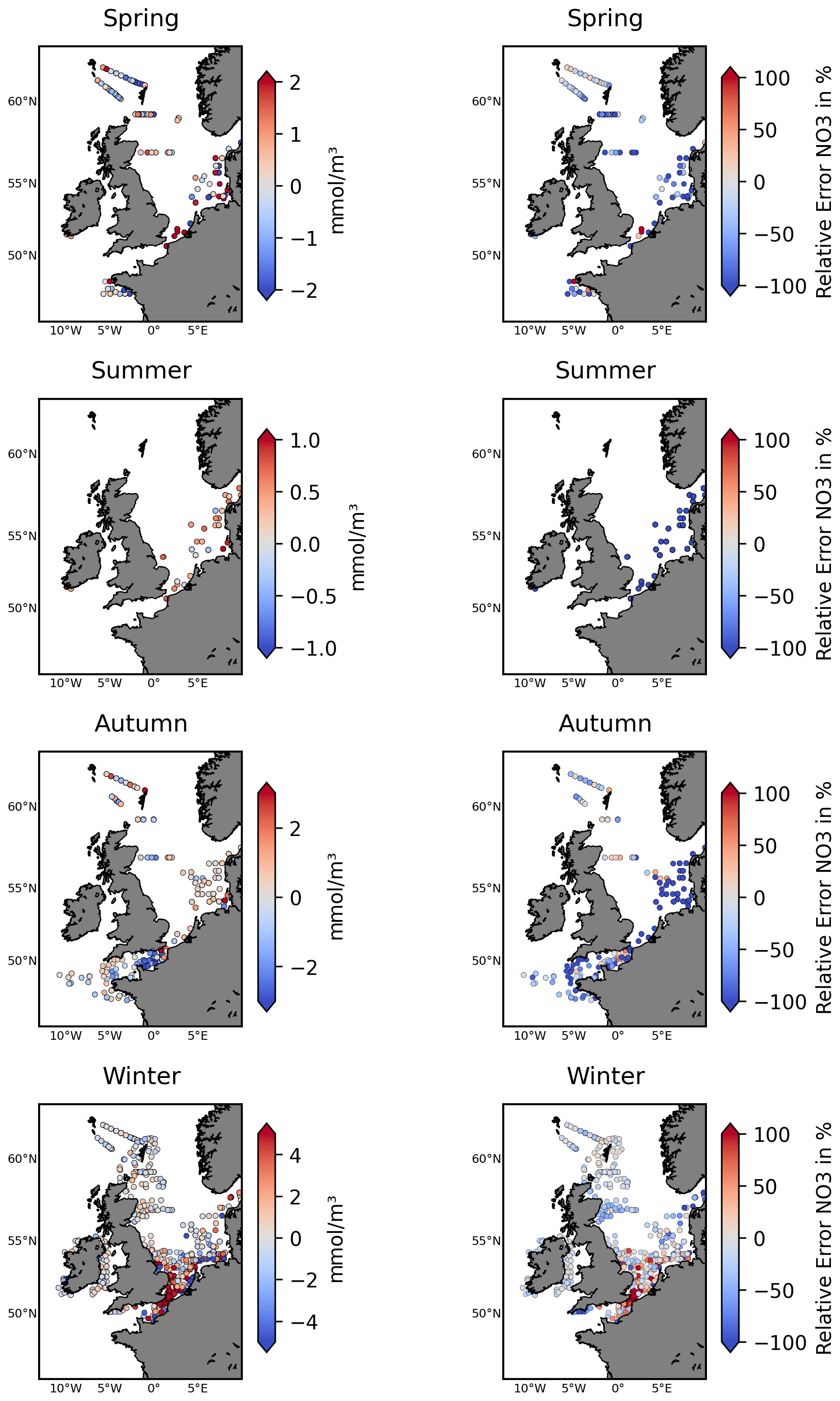
Figure 4 The left-hand panels show the ICES nitrate test data locations for different seasons, with the colour bar accounting for the NN model's skill (difference between predicted and observed nitrate: predicted−observed). The right-hand panels show the relative performance metrics comparing the NN model to the Copernicus reanalysis skill, as defined in Eq. (1). It marks the NN model's improvement (blue) or degradation (red) relative to the reanalysis when compared (in %) to the observed nitrate concentrations.

Table 1 The skill of the NN model in predicting nitrate compared with the Copernicus reanalysis (Kay et al., 2016). Skill is measured by bias (Eq. 2, in mmol m⁻³), the bias-corrected root mean squared error (BC-RMSE; Eq. 3, in mmol m⁻³), and Pearson's correlation (R). The rows represent different test data from ICES and the coastal stations. The last two rows show the skill of the NN model and the reanalysis in predicting interannual, low-pass-filtered time series (for details, see Fig. S3). For the five Scottish stations, we show only the averaged result of all the stations.

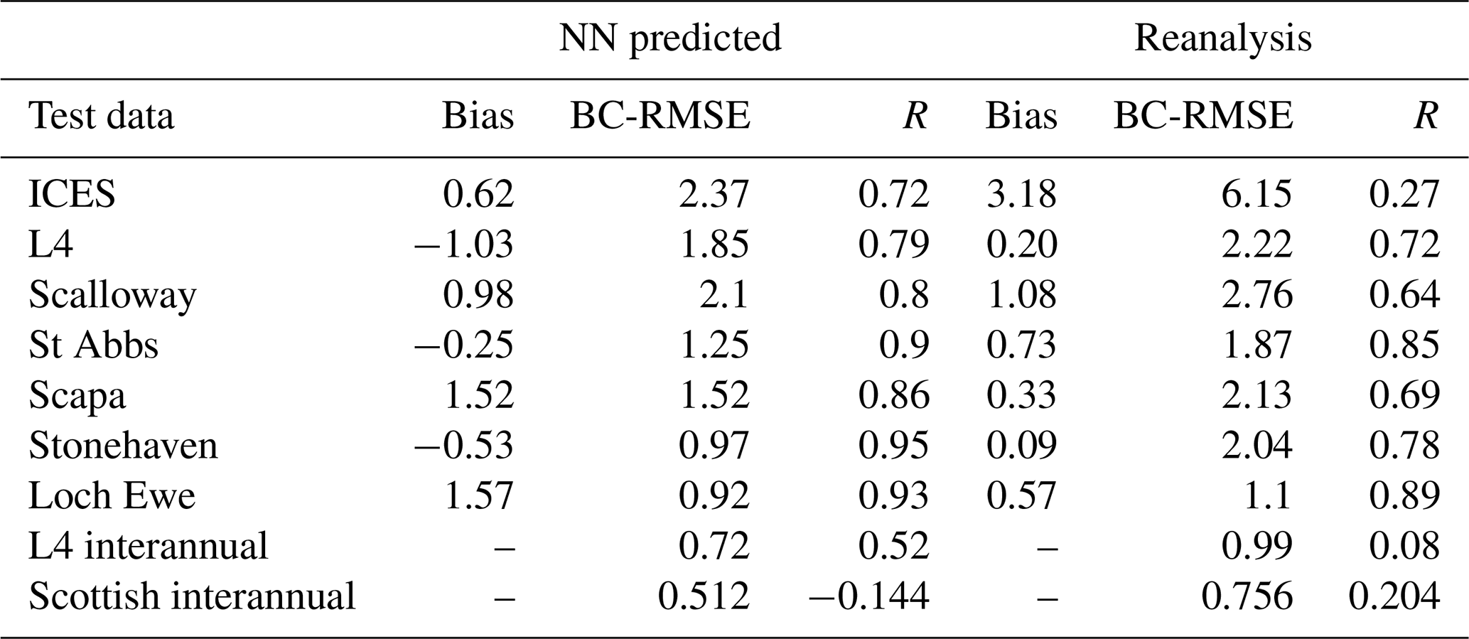
2.3 Skill metrics

We used the relative performance (RP) skill metric to compare the performance of the NN model from this study with the reanalysis:

$$\begin{array}{}\text{(1)}& {\displaystyle }{\displaystyle }\text{RP}(\text{NN},\text{Rean})=\mathrm{100}\cdot {\displaystyle \frac{\left(\right|\text{NN}-\text{Obs}|-|\text{Rean}-\text{Obs}\left|\right)}{\text{Obs}}}.\end{array}$$

In Eq. (1), “Obs” stands for observations, “NN” for predicted values by the NN model, and “Rean” for reanalysis. Negative values of the RP metrics from Eq. (1) indicate that the NN model outperforms reanalysis and vice versa.

The bias between any model, “Mod” (“Mod” could be either NN or reanalysis), and observations is defined as

$$\begin{array}{}\text{(2)}& {\displaystyle }{\displaystyle }\text{Bias}(\text{Mod},\text{Obs})=\langle \text{Mod}-\text{Obs}\rangle ,\end{array}$$

where the averaging 〈…〉 is taken through all the available matching model and observational data.

The bias-corrected RMSE (BC-RMSE) is defined as the RMSE after the bias h has been subtracted from the model:

$$\begin{array}{}\text{(3)}& {\displaystyle }{\displaystyle }\text{BC-RMSE}=\sqrt{〈(\text{Mod}-\text{Obs}-\text{Bias}{)}^{\mathrm{2}}〉}.\end{array}$$

Apart from the metrics from Eqs. (1)–(3), we also used Pearson correlation. Our tests show that the effective temporal resolution of the NN model (timescale on which it performed best relative to the test data) is around 15 d (the tests are not shown here, but some insight is provided by Fig. S3 in the Supplement). We therefore low-pass filtered all the compared data on a 15 d scale before any of the metrics from this section were applied.

3 Results and discussion

3.1 Model validation

Figure 4, Table 1, and Figs. S4–S5 in the Supplement demonstrate that the NN model shows very good skill relative to the test data from ICES, L4, and the Scottish stations and substantially outperforms the existing Copernicus reanalysis product for NWES nitrate. For example, the bias measured by the ICES test data has been reduced by more than 80 % relative to the reanalysis, the BC-RMSE has been reduced by more than 60 %, and the Pearson correlation has increased from 0.27 to 0.72. Comparison to the data from coastal stations shows less consistent improvement in terms of bias relative to the reanalysis, but the NN model still outperforms the reanalysis in BC-RMSE and R at each of the locations.

Because the nitrate time series are dominated by the seasonal signal, it is important to explore whether the model skill extends beyond predicting the local nitrate seasonal (e.g. monthly) climatology. This is much harder to validate, as one needs long-term time series at specific locations, which are rare. We have looked at the data from the L4 station and five Scottish locations to analyse the ML model's skill in capturing interannual variability of nitrate. The results (shown in Table 1 and Fig. S3) are more mixed: at the L4 station, which has the longest time record and richest dataset out of all locations, the ML model performs very well in predicting the interannual nitrate time series. It is interesting that at the same location the reanalysis does a very poor job in doing the same (Table 1). At the Scottish stations, the ML model correctly captures the size of the interannual variability in nitrate, but it struggles to capture the variability itself (the R metrics in Table 1). It is however noteworthy that some of the time series at the Scottish locations are relatively short (see Sect.2.1) and therefore not the most suitable for this type of analysis.

Finally, the test data selected from the ICES dataset are time separated from the training and validation data but are spatially located in largely overlapping regions (see Fig. 2). It is therefore important to explore the possibility that, due to geographic proximity, some ML skill has been transferred from the training and validation data to the test data. This is done in Fig. S6 in the Supplement, showing how the skill evolves as a function of spatial separation between the test data and the training and validation data. Although there is large variability in the skill, Fig. S6 shows no significant trend with spatial distance, indicating that the ML model's skill does not decrease (it even improves slightly) with the increase in spatial separation.

3.2 The bi-decadal nitrate product, trends, variability, and implications

Figure 3 shows the 1998–2020 seasonally averaged NWES nitrate concentrations. It is clear from the spatial nitrate distributions that the NN model does not capture the ∼7 km scale variability sufficiently, including the exact NWES boundaries, but it does capture coarse-resolution nitrate distributions reasonably well (see Fig. 5 for comparison with the World Ocean Atlas (WOA) product of Garcia et al., 2019). Similarly, our analyses (including Figs. S3–S5) suggest that the effective temporal resolution of the NN product is ∼15 d, rather than daily. Figure 3 also provides seasonal comparison with the Copernicus reanalysis product, evaluating the significant reanalysis biases throughout the 1998–2020 period. The Copernicus reanalysis validation gives similar results to the validation from Kay et al. (2016), who compared the reanalysis with the North Sea Biogeochemical Climatology for 1960–2014 (Hinrichs et al., 2017).

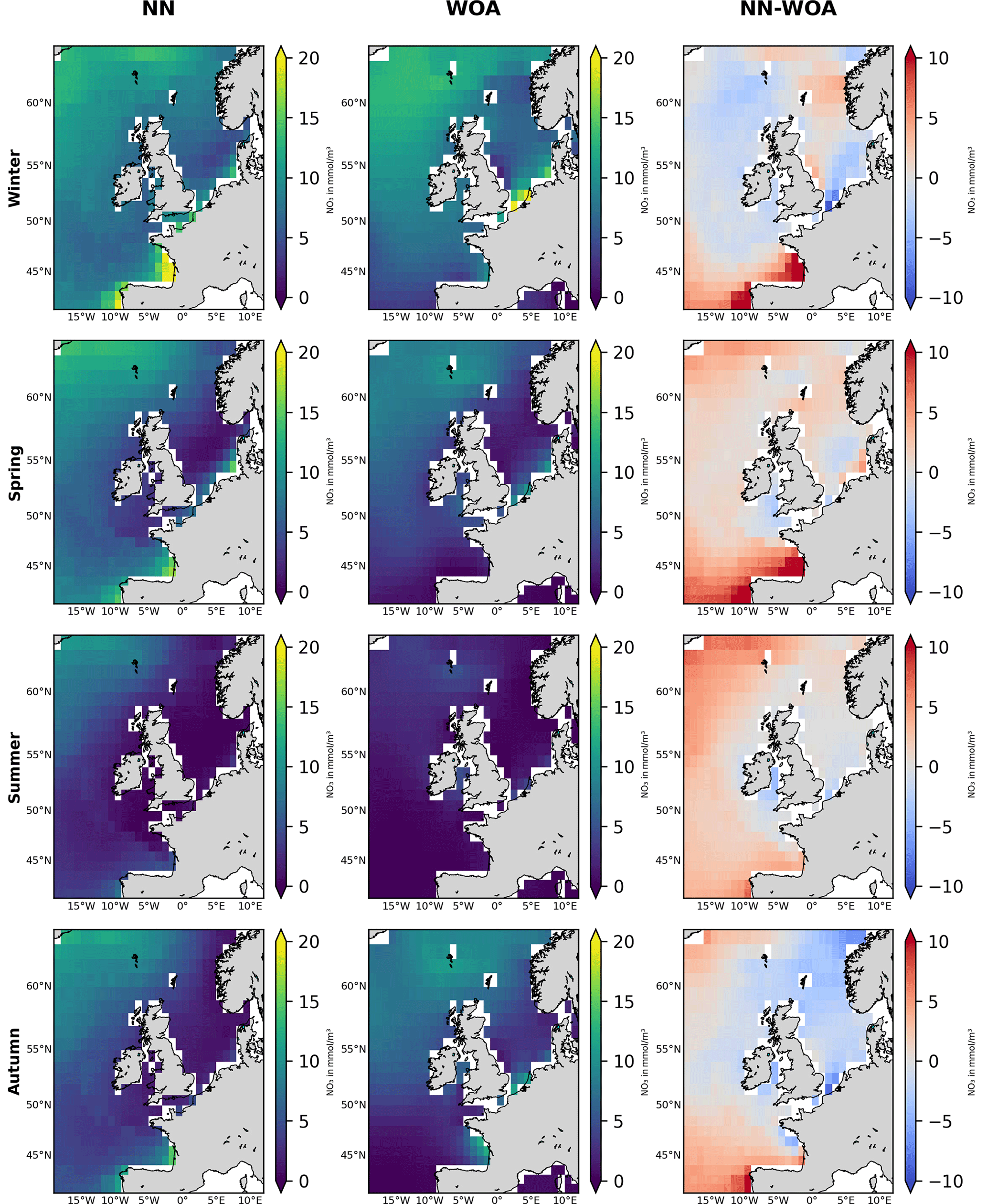
Figure 5 Seasonal comparison of the NN-predicted 1998–2020 surface nitrate averages (left-hand panels) with those of the World Ocean Atlas (WOA) 2018 product (middle panels, Garcia et al., 2019). Right-hand panels show the difference (NN-predicted averages minus WOA product averages) for corresponding seasons. The NN-predicted data are coarse grained on the WOA 0.25° spatial resolution scale. The focus is on spatial nitrate features, rather than nitrate concentration values, as the WOA averages data for the whole 1900–2018 period, including highly eutrophic decades in the 1970s and 1980s.

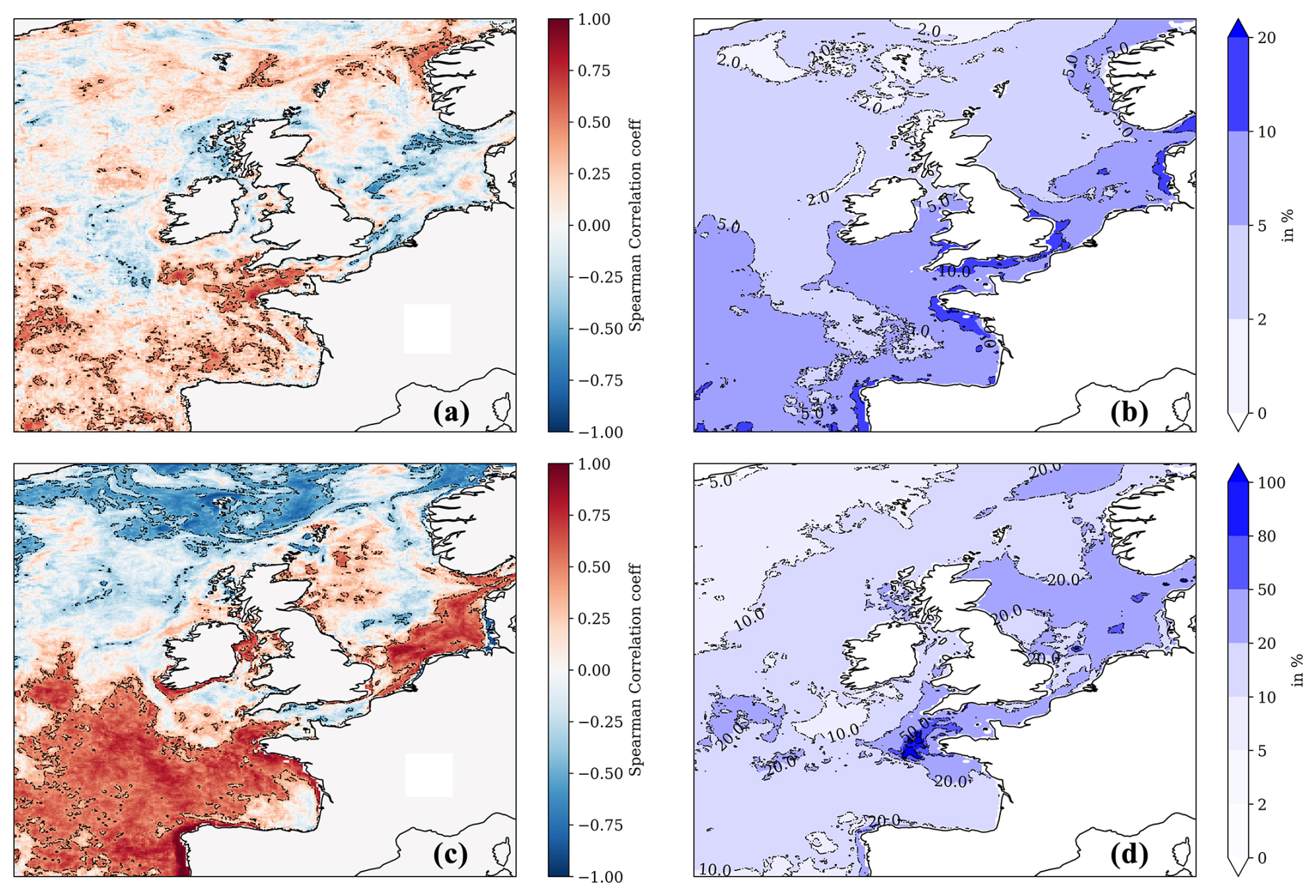
Figure 6 The upper left-hand panel (a) shows the Pearson correlation between the NN-predicted mean winter surface nitrate concentrations and the mean (following) spring surface chlorophyll concentration from the Copernicus reanalysis. The upper right-hand panel (b) shows the interannual variability for NN-predicted winter surface nitrate concentration (for 1998–2020, measured by the standard deviation) relative to the 1998–2020 winter mean (in %). The bottom-left panel (c) is similar to panel (a) but showing the Pearson correlation between the NN-predicted summer surface nitrate concentration and the summer surface total chlorophyll concentration from the Copernicus reanalysis. Panel (d) is the same as panel (b) but showing interannual variability of NN-predicted surface nitrate concentration in the summer rather than in the winter. The dashed contours in panels (a) and (c) show regions where the correlation is statistically significant (p value <0.05).

Winter nitrate concentrations play an important role in the pre-conditioning of the spring bloom, which largely drives the NWES's biogeochemical seasonal cycles (Huisman et al., 1999; He et al., 2011). Winter dissolved inorganic nitrogen is used by OSPAR (in combination with other parameters) in its common procedure (OSPAR, 2005) as an important indicator of NWES eutrophication and the next season's growth (Axe et al., 2017; Topcu and Brockmann, 2021). The hypothesis that the intensity of the spring phytoplankton bloom is directly related to the abundance of nutrients in the winter before the bloom has been investigated here through nitrate.

In Fig. 6a, we find only limited evidence of the relationship between the winter (December–February) nitrate and spring bloom intensity; i.e. a statistically significant positive Pearson correlation has been found only in the western English Channel region, near the shelf break in the Celtic Sea, around the Bay of Biscay, and in the south-west of the model domain (accounting for at most 30 %–35 % of explained variance). Figure 6a also shows that these are regions where the interannual nitrate variability appears to be relatively large (>5 % of the winter average in the majority of the region, with 10 %–20 % in specific sections, Fig. 6b) and therefore capable of revealing a stronger relationship with spring chlorophyll. For most of the domain, there is a lack of clear correlation between interannual winter nitrate and spring chlorophyll, which could be explained by the fact that both are driven by the interannual variability in the atmosphere (Dutkiewicz et al., 2001; Follows and Dutkiewicz, 2001; Ueyama and Monger, 2005; Henson et al., 2006; Zhai et al., 2013). Increased winds can lead to more mixing and elevated surface nutrients, whilst dampening blooms by transporting phytoplankton below the Sverdrup critical depth, as proposed by popular hypotheses explaining the North Atlantic spring blooms (Sverdrup, 1953; Huisman et al., 1999). Furthermore, there is a lack of complete agreement on what the dominant drivers of the spring bloom in the North Atlantic are, and arguments have been raised that support the view that blooms result much more from internal ecosystem dynamics (e.g. zooplankton control over phytoplankton, Behrenfeld and Boss, 2014) compared to what was assumed by traditional hypotheses focusing on physics. It is noteworthy that the weak link between winter nitrate and phytoplankton growth reported here is also consistent with recent results by Van Leeuwen et al. (2023).

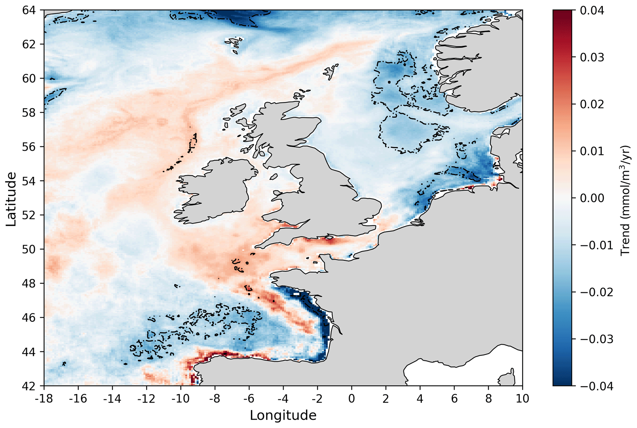
Figure 7 Linear trends at each spatial location in the annual nitrate concentration 1998–2020 time series obtained from the NN model prediction. Dashed contours mark areas with statistically significant trends (p value <0.05).

In Fig. 6c we look at correlations between interannual time series of summer nitrate and chlorophyll concentrations. The high positive correlation in Fig. 6c indicates regions where growth is either strongly nitrate limited or limited by other drivers that are positively correlated with nitrate. Realistically, only other nutrients are likely to act as such drivers, i.e. phosphate (there is substantial phosphate limitation on the NWES, Skogen et al., 2004; Philippart et al., 2007; Loebl et al., 2009; Lenhart and Große, 2018; Burson et al., 2016; Grosse et al., 2017), so we can conclude that those regions are strongly nutrient limited in the summer (with the nutrient likely being nitrate). The coastal part of the regions with strong positive correlation delimits areas which could be more sensitive than others to high river nutrient loads. This does not automatically imply high risk of eutrophication, as this would also depend on other factors, such as the overall river outflow in each area and the socio-economic activity, but it indicates certain increased vulnerability. Figure 6c shows high summer nitrate and positive chlorophyll correlations, mostly in the southern North Sea region, the western English Channel, the Bay of Biscay, and the south-west of the domain. These are again the regions where the interannual fluctuations in summer nitrate are relatively large (Fig. 6d). Interestingly, the eutrophication problem areas, as identified by the OSPAR NWES eutrophication status reports (such as the south-eastern North Sea, coastal areas around Brittany, Axe et al., 2017; Devlin et al., 2023), fall under these vulnerable zones delimited in Fig. 6c. However, Fig. 6c also includes other regions, such as the eastern coastline of Scotland, the southern coast of Ireland, and zones in the Irish Sea.

Finally Fig. 7 shows 1998–2020 trends in winter nitrate concentration over the NWES domain. In most of the domain, no statistically significant nitrate trends have been detected, but some small negative trends (∼0.02 mmol m⁻³ yr⁻¹) were found in the southern North Sea and the north-east region near the Norwegian trench. Somewhat larger (∼0.08 mmol m⁻³ yr⁻¹) statistically significant negative trends have been found in specific locations of the Bay of Biscay. These results (e.g. from the southern North Sea) are broadly consistent with what has been reported for this period in the recent OSPAR report (e.g. Axe et al., 2017, 2022). These small trends may follow the smaller rates of reduction in the nitrate riverine inputs during the data period (1998–2020) compared to their large reduction in the 1980s and earlier 1990s (Duarte, 2009; Brockmann et al., 2018; Greenwood et al., 2019). However, it should be noted that significant reduction in atmospheric nitrogen input has been reported in the last few decades (Devlin et al., 2023).

4 Conclusions

In this work we have demonstrated that, using sparse observations across the North-West European Shelf (NWES), machine learning (ML) can be a powerful tool to reconstruct a spatially complete sea surface nitrate dataset over a period of 23 years. We have shown that the dataset has substantially better match-ups with independent test data than the existing NWES nitrate reanalysis. Using the newly developed product, we have identified nutrient-limited coastal areas with potentially strong ecosystem responses to an event of river nutrient pollution, addressed nitrate decadal trends, and tested how successfully winter nitrate can be used as a predictor of the phytoplankton spring bloom. The areas of strong ecosystem response to nutrient loads were identified as the south-east of the North Sea, the coastline of Brittany, and the Bay of Biscay (areas previously marked by OSPAR as eutrophication problem areas, Axe et al., 2017; Devlin et al., 2023), but additional coastal areas were also identified in the south of Ireland, the eastern Scottish coastline, and the Irish Sea. We have found that nitrate trends in the last 2 decades were mostly minor, with the exception of the coastline in the Bay of Biscay. This confirms recent observations by Axe et al. (2017, 2022) and Devlin et al. (2023). We have also demonstrated that winter nitrate is only a limited predictor of the next season's growth, which again supports recent findings of Van Leeuwen et al. (2023).

There are many other potential scientific uses for the nitrate dataset; e.g. we propose assimilating the nitrate data into the NWES operational model to correct the model's significant nitrate biases, potentially improving its dynamics and its short-range forecasts. The model's skill in simulating phytoplankton is known to quickly degrade with the forecast lead time (e.g. Kay et al., 2016; Skákala et al., 2018), and biases in nitrate might be one of the leading factors in driving this. Assimilation of nitrate products derived here will be addressed in the near future.

Several extensions of this work would also be desirable, such as utilising ICES data for other biogeochemical indicators to produce ML-informed multi-variate datasets across the whole NWES domain (these should include other nutrients and oxygen). ML could also identify valuable patterns of relationships across the multiple variables. Furthermore, the model developed here did not show very good skill in capturing high-frequency (daily) temporal variability, including extreme events. This might be due to processes providing the ocean with a memory that is significantly longer than the daily timescale of the product. Representing ocean memory by the NN model might require using time-lagged input features, which could substantially inflate the size and the complexity of the model. Despite this, including such features into the NN model should be considered in the future, i.e. also with respect to developing a more realistic river discharge advection scheme than the one used here, which is a major challenge. Interestingly, the finer spatio-temporal representation of nitrate could be automatically improved if we assimilated the NN-predicted nitrate into the dynamical model, as such a scheme would benefit from both the dynamical model advection scheme and the improved representation of the (coarser-resolution) nitrate by the NN model. Other future activities should include re-training the NN model whenever newer and potentially better observational products appear for its inputs (such as new riverine discharge data appearing in the last few years, van Leeuwen and Lenhart, 2021). Finally, ML tools designed to specifically capture extreme phenomena can be deployed in the future and extend the applicability of this work.