Groundwater–CO₂ emissions relationship in Dutch peatlands derived by machine learning using airborne and ground-based eddy covariance data

Peatlands worldwide have been transformed from carbon sinks to carbon sources due to years of intensive agriculture requiring low water tables. In the Netherlands, carbon dioxide (CO₂) emissions from drained peatlands mount up to 5.6 Mton annually and, according to the Dutch climate agreement, should be reduced by 1 Mton by 2030. It is generally accepted that mitigation measures should include raising the water level, and the exact influence of water table depth has been increasingly studied in recent years. Most studies do this by comparing annual eddy covariance (EC) site-specific CO₂ budgets to mean annual effective water table depths. However, here we apply a different approach: we integrate measurements from 16 EC towers with EC measurements from 141 flights by a low-flying research aircraft in an interpretable machine learning (ML) framework. We make use of the different strengths of tower and airborne data, temporal continuity, and spatial heterogeneity. We apply time frequency wavelet analysis and a footprint model to relate the measured fluxes to the underlying surface. Using spatiotemporal data, we train and optimize a boosted regression tree (BRT) machine learning algorithm to predict immediate CO₂ fluxes and use Shapley values and various simulations to interpret the model's outputs. We find that emissions increase by 4.6 t CO₂ ha⁻¹ yr⁻¹ (90 % confidence interval: 4.0–5.4) for every 10 cm lowering of the water table, down to a water table depth of 0.8 m below the surface. For more drained conditions, emissions decrease again. Furthermore, we find that the sensitivity of CO₂ emissions to drainage is stronger in winter than in summer and that it varies between sites. This study shows the added value of using ML with different types of instantaneous data and holds potential for future applications.

1 Introduction

Despite covering only 3 % of the earth's land surface, peatlands store around 25 % of all terrestrial carbon and play a crucial role in the global carbon cycle (Yu et al., 2010). They are the most carbon-dense ecosystems of the terrestrial biosphere and have a true potential for climate change mitigation (Leifeld and Menichetti, 2018; Loisel et al., 2021). In natural, waterlogged fens and bogs, uptake of carbon dioxide (CO₂) through vegetation and subsequent sequestration in peat soils abundantly exceeds the emission of methane (CH₄) (Frolking and Roulet, 2007). However, peat soils have been exploited and drained worldwide for fuel extraction and agricultural practices. They widely transformed from carbon sinks to carbon sources due to increased peat decomposition following higher oxygen availability and are currently responsible for large CO₂ emissions.

The Netherlands has a long history of peat extraction and intensively draining peatlands for agriculture and livestock farming (van den Akker et al., 2008; Erkens et al., 2016). This has led to increased carbon dioxide emissions, currently accounting for ∼ 3 % of all Dutch emissions (5.6 Mton annually), and land subsidence, which in turn increases the need for further drainage (Kwakernaak et al., 2010; Ruyssenaars et al., 2022). To counter this spiral, the Dutch government set a specific mitigation target for peat meadows: annual emissions must be reduced by 1 Mton by 2030 (Government of the Netherlands, 2019). It is generally accepted that countermeasures to reduce such emissions should include raising the water table, as the water table seems to be the predominant control on greenhouse gas emissions from managed peatlands (Evans et al., 2021). However, the exact impact of higher groundwater levels on CO₂ fluxes is not yet entirely established and has been increasingly studied in the past years (Aben et al., 2024; Boonman et al., 2022; Evans et al., 2021; Fritz et al., 2017; Kruijt et al., 2022; Tiemeyer et al., 2020).

Studies investigating agricultural systems generally require correcting the annual net ecosystem exchange (NEE) for lateral movement of carbon associated with manure applications and harvests and relate the resulting net ecosystem carbon balance (NECB) to the mean annual groundwater level (Aben et al., 2024; Boonman et al., 2022; Evans et al., 2021; Kruijt et al., 2022). In unmanaged systems, annual NEE is equivalent to NECB. Averaging out daily and seasonal variation, the goal is to isolate the underlying effect of groundwater level. This way, multiple studies found linear relationships with similar slopes: between 2.1 and 4.5 t CO₂ ha⁻¹ yr⁻¹ extra emissions per 10 cm increase in WTDe (Boonman et al., 2022; Evans et al., 2021; Fritz et al., 2017; Jurasinski et al., 2016; Kruijt et al., 2022). Tiemeyer et al. (2020) fitted the Gompertz function to a set of annual balances, which shows a sharper increase in emissions at shallow water levels but then saturates at around 0.4 m. Recently, multiple studies have applied this function (Friedrich et al., 2024; Koch et al., 2023; Nijman et al., 2024).

While studies on annual budgets provide valuable insights into the underlying groundwater–CO₂ relationship and differences between sites, some limitations emerge. First, to obtain an NECB estimate for any location, year-round data at that specific location are required, which is not always achievable and generally requires some trustworthy gap filling. Second, whilst carbon import and export can add up to significant amounts, these numbers are often hard to obtain and generally unavailable at landscape level. Third, the site comparisons are robust only when comparing sites with markedly different average water table depths. The datasets used have been based on site-specific observations, with well-defined, fairly homogeneous soil and vegetation characteristics and well-known water table management. However, these factors generally vary widely on the regional scale. Last, the annual estimates discard possibly important information from intra-annual variability and relationships with factors other than groundwater. In the current study, we aim to bypass these limitations by alternatively exploring the short timescale at the regional level to further unravel the influence of water table depth and other key drivers on CO₂ emissions from agricultural peatlands in the Netherlands.

We do this by incorporating flux measurements from a low-flying aircraft. Airborne measurements bear high spatial heterogeneity, since every measured flux originates from an area called the footprint spanning several kilometers, and an entire region can be covered by an appropriate flight pattern. However, a limitation of the airborne measurements is that they are generally limited to daytime conditions. This limitation is particularly critical for CO₂ studies, given the different contributions of gross primary productivity (GPP) and ecosystem respiration (Reco) to NEE. Here, we are specifically interested in the peat decomposition component of heterotrophic respiration, unrelated to GPP. Measurements by eddy covariance towers, however, are continuous and include nighttime fluxes, enabling NEE partitioning, but are limited by their fixed location. Therefore, we consider the complementary use of tower and airborne flux estimates to be essential to assess CO₂ fluxes at a regional scale.

Airborne measurements (integrated flux signals from their respective footprints) can be related to the underlying surface by environmental response functions using either more classical statistical methods (Hutjes et al., 2010) or artificial intelligence approaches (Metzger et al., 2013, 2021; Serafimovich et al., 2018). Both depend on laying the footprint of all flux measurements over maps of vegetation, land use, and soils and/or direct satellite-derived products. Here, we integrate tower and airborne data using the “LTFM” approach initially developed by Metzger et al. (2013). The acronym stands for low-level flights (L), time frequency wavelet analysis (T), footprint modeling (F), and machine learning (M). We aim to apply this machine learning (ML) approach to identify key predictors of NEE and understand their influence on CO₂ dynamics in Dutch peatlands.

Today, peat soils in the Netherlands can be found in the “Groene Hart” and in the provinces of Friesland and Overijssel. These areas share similarities, such as being mostly dominated by pastures with ditches, but also differ in certain respects, such as average drainage depth, Friesland being the most intensively drained with the lowest water tables. In the current study, we have three distinct flight tracks: above the Groene Hart area, in southern Friesland, and in the western part of Overijssel. These three regions are also equipped with flux towers, and thus we measure both airborne and tower CO₂ fluxes from all three.

In our aim to understand the influence of key predictors, we inspect potential differences and similarities between these areas. We do this by building several models: one model based on all data together and models per area separately trained only on the data of the respective area. We expect the model with all data will perform best, since in machine learning data quantity is often a determining factor for performance. Furthermore, we expect that although characteristics of the areas vary, the underlying processes do not; hence, “one model fits all”, and area-specific models can be used to predict for other areas. To achieve physical interpretability of our ML approach, we use the SHAP framework and model simulations, fully exploring the identified relationships. We hypothesize that, alongside drivers of the diurnal cycle, water table depth plays an important role at the regional scale in all areas and that the machine learning approach can help us to better understand drivers of CO₂ fluxes. We aim to finally create a robust, interpretable ML model that can be used in the Netherlands to predict CO₂ emissions from drained fen meadows at a regional scale.

2 Methods

In this study, we merge airborne flux measurements with ground-based eddy covariance (EC) measurements to make use of their spatial and temporal strengths, respectively. Both are part of the intensive monitoring network implemented by the Netherlands Research Programme on Greenhouse Gas Dynamics in Peatlands and Organic Soils (NOBV, https://www.nobveenweiden.nl/en/ last access: 20 May 2025), that was established following the Dutch mitigation target of 2019. The goal of the NOBV is to further understand greenhouse gas emissions from drained fen meadows, their drivers, and the efficiency of proposed mitigation measures. Here, we test a machine learning approach on the combination of airborne and tower data to assess the most important drivers of CO₂ emissions on a regional level and to quantify the influence of water table depth.

In Fig. 1, a visual overview of the methodology is shown, which can be roughly split up into three parts: data collection and data processing, building and optimizing several machine learning models, and interpreting the results with Shapley values and simulations. In this section, we describe these three parts of our approach.

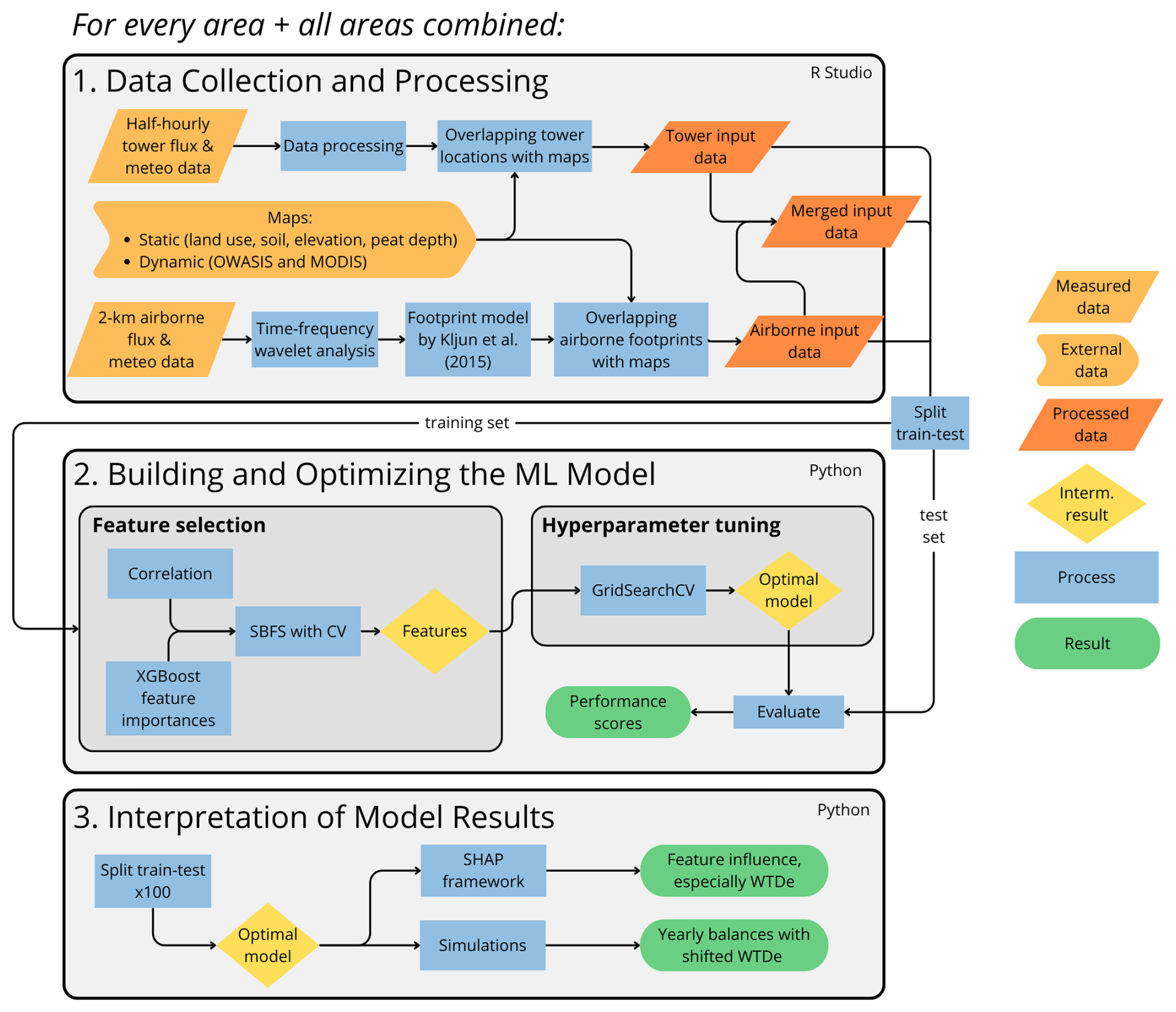
Figure 1 Methodological steps for the current study. We divide the methods into three main parts: (1) data collection and processing, (2) building and optimizing the machine learning (ML) model, and (3) interpretation of model results. We carried out all steps for the three study areas separately, i.e., for the Groene Hart, southern Friesland, and the western part of Overijssel (see Fig. 2), as well as for all areas combined. Sources for external data can be found in Table 2; more details on data processing can be found in Sect. 2.1.3 and Appendix A. All steps are described in the text.

2.1 Data collection and processing

2.1.1 Study area

The study area comprises the three main peat soil areas in the Netherlands: the Groene Hart in the southwest of the country, southwest Friesland, and the “Kop van Overijssel” south of that (see Fig. 2). These peat areas were entirely formed during the Holocene, reaching their maximum extent (about 50 % of present Netherlands) around 4000 years ago. Between 2000 and 1000 years ago, large tracts eroded away by a rising and repeatedly intruding sea. Since medieval times, peat has been extracted by humans, and the land has been drained for agricultural purposes. Peat mining continued at a large scale until the late 19th century, while drainage continues to this day (Erkens et al., 2016; van Asselen et al., 2020). Most remaining peatlands are fens, and the very few that can be characterized as bogs are not the subject of this study. The fen meadows are primarily used as pastures for dairy farming and currently cover around 7 % (ca. 290 000 ha) of the Dutch land surface (Arets et al., 2018). Water table depth in the study area ranges from the surface level to 150 cm below the surface level, with most deeply drained soils in Friesland. The climate is temperate and humid, and the Dutch Meteorological Institution states mean annual temperatures between 9.5 and 11.5 °C and annual precipitation between 670 and 1100 mm (KNMI, 2024).

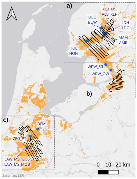
Figure 2 The EC tower network used in this study, with three flight tracks over the study areas: (a) Friesland, (b) Overijssel, and (c) Groene Hart. Peat distribution is shown in orange. Airborne fluxes are calculated over the entire flight tracks, including the turn, since the banking angle was kept less than 15°. General information on the EC sites and processing can be found in Sect. 2.1.3 and Appendix A. For more detailed, site-specific information, see Kruijt et al. (2022). The map was made in QGIS using an ESRI base map; peat distribution was obtained from the soil map (Wageningen Environmental Research, 2024).

2.1.2 Airborne flux measurements

The aircraft used is a SkyArrow 650 TCNS, a lightweight environmental research aircraft with a push propeller. Weather permitting, i.e., with good visibility and no rain, surveys were done twice a week between March 2020 and December 2023, alternating between the three areas described above. However, between July 2020 and February 2021 and between November 2022 and June 2023, the aircraft did not fly due to technical issues. In total, we used data from 141 flights. Parallel flight tracks 2–3 km apart were designed perpendicular to the prevailing wind direction and landscape gradients to get complete spatial coverage of the area of interest. Figure 3 shows a typical flight trajectory. Mean flying altitude was 60 m, so built-up areas had to be avoided. The flight transects covered all major soil and land use classes, although the footprints were mostly dominated by pastures on peat soils – as are the areas.

The aircraft was equipped with an open-path gas analyzer for CO₂ and latent heat fluxes and a thermocouple for sensible heat, both depending on a BAT probe for 3D wind speed and momentum flux. In addition, net radiation, incoming and reflected photosynthetic active radiation (PAR), and air and surface temperature were measured. Most instruments sampled at either 50 or 20 Hz. More detail on the aircraft and its equipment can be found in Vellinga et al. (2013). Post-flight processing started with de-spiking raw data. Next, 50 Hz air pressure and temperature measured by the BAT probe were converted to 3D wind fields and corrected for all aircraft motions. Then, covariances between wind and CO₂ concentrations were calculated. Conventionally, covariances are calculated over time and then spatially integrated over a fixed window, for example 2 km long. However, varying conditions can require different window lengths (Sun et al., 2018). Furthermore, this block averaging method potentially suffers from spectral losses and reduced statistical precision at lower frequencies, as is the case with tower-based measurements using typical averaging times (Paleri et al., 2022). As in Metzger et al. (2013), we used wavelet cross-scalograms calculated over the entire flight to find covariances in the frequency domain: smaller-scale, local turbulent fluxes at high frequencies and larger-scale mesoscale contributions at low frequencies with large wavelengths. Wavelengths larger than the boundary layer height were discarded. The fluxes at these two scales are then summed in non-overlapping 2 km windows to get the flux over all scales. Further processing including quality checks and u_* filtering was done following the framework of Foken et al. (2004). In Appendix A we provide an overview of the applied steps. In addition, the most important meteorological scalar variables were also averaged over a 2 km spatial window.

To determine the spatial origin of the airborne measurements, the flux footprint model by Kljun et al. (2015) was used. This two-dimensional source weight function is a parameterization of the backward Lagrangian model and describes the spatial extent, position, and distribution of the contributing surface area. The function can be applied to wide-ranging boundary layer conditions and has been widely used by studies dealing with airborne flux observations (Hannun et al., 2020; Sun et al., 2023). The input parameters include Obukhov length (L), standard deviation of lateral wind velocity (σ_v), measurement height (z_m), and friction velocity (u_*), which were measured directly by sensors on the aircraft, and planetary boundary layer height (h), which was extracted from the ERA5 product. Roughness length (z₀) is implicitly included in the footprint model by the fraction $u\left(z_{\mathrm{m}}\right)/u_{*}$ (Kljun et al., 2015).

For every 2 km window, five overlapping sub-footprints were calculated and overlaid with various maps, described below. A typical flight with all sub-footprints is shown in Fig. 3. For maps with continuous values, weighted averages were computed, whereas for categorical maps, the fraction of each category in the footprint was calculated. To obtain the final contributions to the flux measurements, the sub-footprints were combined and normalized. Footprints with more than 15 % of built-up area were excluded (discarding 17 % of airborne data), as well as footprints where the dominant land use class is anything other than “grasslands”, “fens and bogs”, or “summer crops” (discarding 3 %). Finally, we had around 10 400 airborne data entries.

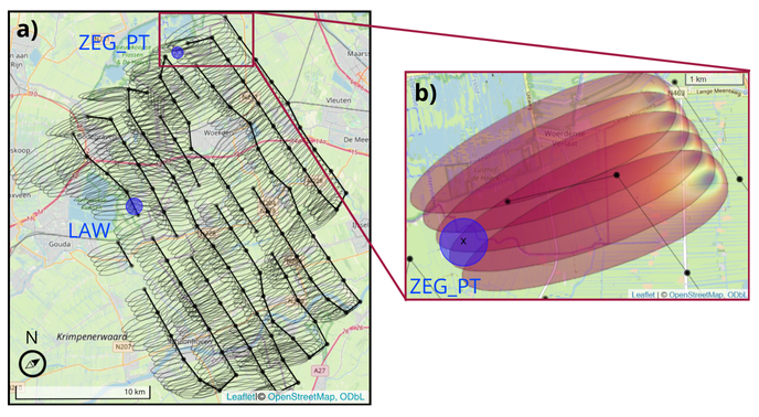
Figure 3 Airborne sub-footprints of a typical flight over the Groene Hart, with flight altitude of 60 m. In this study, we used static circular footprints for towers, which are shown in blue for LAW and ZEG_PT. In (a), five sub-footprints are visible for every 2 km window, where the contour lines represent the area from which 80 % of the measured flux originates. All sub-footprints were overlaid with spatial data and subsequently combined and normalized to get the final footprint values. The wind rose shows the average wind direction. In (b), we show the contribution distribution within the first five sub-footprints: blue indicates the highest contribution, and red indicates the lowest. The black “x” denotes the ZEG_PT tower location. In both (a) and (b), the differences in tower and airborne footprints are visualized.

2.1.3 Eddy covariance towers

The NOBV implemented an intensive monitoring network of EC towers (see Fig. 2). They are distributed over the three main fen meadow areas mentioned previously and cover a representative range of soil types and water levels. For site descriptions and specifics, as well as the processing of the raw tower data, see the report by Kruijt et al. (2022); below, we use the same site abbreviations.

We used four measurement sites in the Groene Hart (LAW_MS_MOB, LAW_MS_ICOS, DEM, ZEG_PT), 10 in Friesland (ALB_RF, ALB_MS, AMM, AMR, BUW, BUO, HOC, HOH, LDC, LDH), and two in Overijssel (WRW_SR, WRW_OW). Although most of these sites are on agriculturally used land, the two sites in Overijssel are in a relatively wet nature area. We used data covering the period from 16 May 2020 to 31 October 2022, although it should be noted that sites vary in data availability.

At these towers, fluxes of CO₂ (and CH₄, evaporation, and sensible heat, but not considered here) are measured with the EC method, alongside weather station measurements of photosynthetically active radiation (PAR), four-component radiation (shortwave and longwave, incoming and reflected), air temperature, relative humidity (RH), rainfall, soil moisture, and soil temperature. All sites were equipped with open-path gas analyzers, except LAW_MS_ICOS, which used a closed-path CO₂ sensor. Otherwise, sensor setups were identical. The equipment was mounted on top of telescopic masts and arranged perpendicular to prevailing southwest winds. Measuring height ranged between 1.5 and 6 m based on the desired footprint size. Half-hourly fluxes were calculated using EddyPro (LI-COR Biosciences, 2023) and subsequently post-processed using a series of filters (see Appendix A). All processing was streamlined across towers, and no attempts at gap filling were made. Outliers defined as the 0.5 % highest and lowest values after filtering for CO₂ flux were removed, resulting in 66 400 half-hourly data records in total. In Fig. 4, part of the measurement period in Friesland is shown, comparing monthly airborne data to monthly daytime tower data across multiple sites. Although the airborne and tower data can never be compared directly due to intrinsic differences in footprint sizes, the seasonal trend and magnitude of the NEE fluxes are similar. Moreover, for most months the aircraft data are within the range observed by the towers, with both towers exhibiting monthly fluxes lower than aircraft and towers showing monthly fluxes larger than observed by the aircraft. This suggests that the aircraft measured a truly mixed signal.

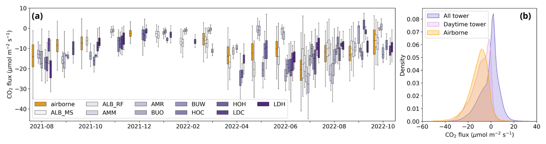
Figure 4 (a) Airborne and “daytime” tower measurements between 10:00 and 16:00 CET (UTC + 1) of CO₂ fluxes in Friesland, binned per month. Boxes represent interquartile ranges, and whiskers show minimum and maximum values, excluding outliers. Only a sub-period of the entire dataset is shown. (b) Probability distributions of airborne and tower data for all areas combined. Here, we use the same time frame for “daytime” as in (a). The airborne and tower fluxes show similar resemblance in the Groene Hart and Overijssel (not shown here).

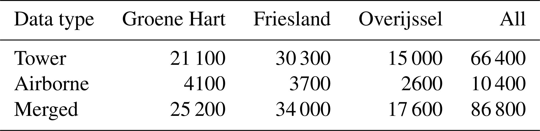
Similarly to the airborne data, the tower data were overlaid with various maps, but without using the footprint model by Kljun et al. (2015). We expected the differences between individual 30 min tower footprints to be negligible compared to the airborne footprints, so we set a fixed circular footprint for every tower (see Fig. 3). The radius was based on the average 80 % of the footprint distance, which was given in the dataset. This footprint was used to extract corresponding spatial data with high spatial resolution (< 200 m). Because of relatively consistent study sites (i.e., flat pastures) and relatively low towers (up to 6 m), the areas within these footprints were largely homogeneous, with the exception of ditches, which were not accounted for. For maps with spatial resolution as low as 250 m, the average value within a radius of 500 m from the measurement point was taken (including > 12 grid cells) because the value from a single grid cell could erroneously deviate from surrounding grid cells. Table 1 shows the final amount of data.

Table 1 Number of data points per data type and area, rounded to the nearest hundred. The “merged” datasets consist of the airborne and tower datasets.

2.1.4 Supplementary surface data

Additional surface data potentially explaining CO₂ flux variations were gathered from various sources, including both static and dynamic maps (see Table 2). Static maps generally had a high spatial resolution (5–25 m) and included land use, soil, peat depth, and elevation. Water-related information was retrieved from the operational product OWASIS by Hydrologic (2019), which consisted of three daily maps: ground water level with respect to sea level (m BSL), soil moisture in the root zone (mm), and air-filled pore space in the unsaturated zone (mm). This product is at national scale with a spatial resolution of 250 m and is based on the national hydrological model (LHM, Ligtenberg et al., 2021). It is made operational by including evaporation and precipitation data, and it is the only water information product covering the entire study area. It performs well in showing trends, but the absolute pixel-based accuracy is up for discussion, and thus we consider a wider area than a single pixel. Lastly, two vegetation indices were retrieved by remote sensing from MODIS: the normalized difference vegetation index (NDVI) and the enhanced vegetation index (EVI). Satellites Aqua and Terra, each with 16 d revisit time, were combined and linearly interpolated to obtain daily values.

(Hazeu et al., 2023)(Wageningen Environmental Research, 2024)Actueel Hoogtebestand Nederland, 2025(Rijkswaterstaat, 2019)Wageningen Environmental Research, 2015(Brouwer et al., 2023)Didan, 2025(Didan, 2021)Didan, 2025

Table 2 Overview of supplementary data sources. For comparison, tower heights ranged between 1.5 and 6 m, with footprints spanning several hundred meters; airborne flying altitude is 60 m, with footprints spanning several kilometers (see also Fig. 3).

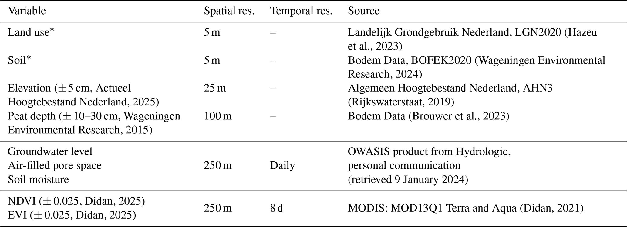
^* Variables with an asterisk are categorical.

The categories of the land use and soil maps were reclassified to obtain a smaller but representative number of variables (see Appendix B). Using the collected information, some additional covariates were calculated, such as effective water table depth (WTDe) based on groundwater level and elevation (Eq. 1), the percentage of all peat classes together present in the footprint (AllPeat), and all peat on sand and peat on peat classes (Eq. 2). Combining peat depth with WTDe, the peat exposed to air (“exposed peat depth”) in centimeters was calculated (Eq. 3).

$$\begin{array}{}\text{(1)}& {\displaystyle }{\mathrm{WTD}}_e=\mathrm{elev}.-\mathrm{OWASIS}\mathrm{\_}\mathrm{GW}\text{(2)}& {\displaystyle }\mathrm{AllPeat}=\sum _{i=\mathrm{1}}^n\mathrm{peat}{\mathrm{class}}_i\text{(3)}& {\displaystyle }\mathrm{ExpPeatDepth}=min(\mathrm{PeatDepth},{\mathrm{WTD}}_{\mathrm{e}})\end{array}$$

WTD_e is effective water table depth below surface level, elev. is elevation, OWASIS_GW is groundwater level below sea level, peat class represents the fraction of the footprint in peat soil class i, and ExpPeatDepth is exposed peat depth or peat exposed to air. Equation (2) was also used to sum only peat on peat classes and peat on sand classes (see Appendix B2 for soil classes).

2.2 Building and optimizing the machine learning model

For every area, as well as for all areas combined, we built a machine learning model based on the combination of tower and airborne data. We used boosted regression trees (BRTs), as they are increasingly used in environmental studies and are furthermore recommended by studies analyzing airborne flux measurements (Metzger et al., 2013; Serafimovich et al., 2018; Vaughan et al., 2021). The package XGBoost (eXtreme Gradient Boosting) was used due to the high predictive performance and computing speed (Nielsen, 2016).

For all sets of input data, we made a train–test division. Commonly, this is done in a random manner, but in our case, because of time dependency of the data and the potential for data leakage, this is not recommended. For the airborne data, we created the test set by randomly selecting individual flight legs. For the tower data, we divided the data in blocks of 4 weeks using the first 3 for training and the fourth for testing. We ensured that the final data distribution was around 80 % training and 20 % testing. We expected this to be a good trade-off between avoiding data leakage and keeping enough data for training. Furthermore, all features in the training set were normalized. The features in the test set were scaled accordingly based on the statistical properties of the training set.

For each model, the model was tuned in two steps: (a) reducing the number of explanatory variables: “feature selection” and (b) optimizing the model's settings: “hyperparameter tuning”. Feature selection was done in a hybrid manner, as is frequently done by studies that use XGBoost (Ogunleye and Wang, 2019; Prabha et al., 2021; Sang et al., 2020; Wang and Ni, 2019). First, we analyzed Pearson correlations to roughly select features correlated with CO₂ and to reject inter-correlated features. Second, feature importances embedded in XGBoost were computed. These first two steps served as a pre-selection of features for the third, more extensive method: sequential backward floating selection (SBFS). SBFS includes an extra “floating” element compared to the more standard and widely used sequential backward selection (SBS) and is known to give good results (Chandrashekar and Sahin, 2014; Rodríguez-Pérez and Bajorath, 2020). SBFS is more time costly than SBS but simultaneously reduces the risk of missing important feature combinations due to early dropping of a specific feature. SBFS was run with 5-fold cross-validation. The model used was an XGBoost tree with n_estimators = 1000, learning_rate = 0.05, max_depth = 6, and subsample = 1, and the scoring metric for the algorithm was RMSE. As there are multiple features describing water dynamics, several options were run separately, excluding inter-correlated features in the same run. To avoid unequal representation in different folds of the cross-validation, all datasets were shuffled beforehand. To evaluate which subset of features is optimal, the R², MSE, bias, and variance of each model proposed by SBFS were computed, and model parsimony was taken into account. The finally selected features are photosynthetically active radiation (PAR), surface temperature (T_sfc), relative humidity (RH), enhanced vegetation index (EVI), effective water table depth (WTDe), and peat depth.

After optimization of the feature subset, the following hyperparameters were tuned: number of trees (n_estimators), maximum depth (tree complexity, max_depth), learning rate (learning_rate), minimum sum of instance weights in a leaf node (min_child_weight), the ratio of columns when constructing each tree (colsample_bytree), and the ratio of instances in every boosting iteration (subsample). We performed a grid search with 5-fold cross-validation (GridSearchCV from scikit-learn) on the training set, and the parameter grid is shown in Appendix C. The R² was used as a scoring metric. In addition, we set a monotone constraint on the model to find a negative relationship between PAR and CO₂ flux such that increasing PAR leads to more negative fluxes. Finally, the model with optimized parameters was evaluated using the test set. Here, based on performance metrics, model parsimony, and usability, the final models were selected for each area. To compare the models' power and found relationships from different areas with each other, we also tested models between areas using the same set of features.

2.3 Interpretation of model results

As we assume the underlying physical processes steering NEE fluxes are the same, we expect that a model trained on one area can be extrapolated to another. However, we expect the Overijssel model to be different, as all tower measurements in this region are from natural areas, unlike in the Groene Hart and Friesland, where sites are located on agricultural land. Although the Overijssel aircraft flux data cover agricultural land, the number of airborne data points is limited compared to the tower data (see Table 1).

Beyond optimizing the model for the best CO₂ predictions, we wanted to understand the model's functionalities and decisions to infer knowledge on the underlying processes. Here, we used two approaches: the explainable AI tool SHapley Additive exPlanations (SHAP) and annual simulations at our site locations. For uncertainty quantification of these interpretations, we applied bootstrapping: we repeated the partitioning in training and testing sets 100 times through a randomized parameter in the splitting algorithm. We created 100 models based on these training sets and used the outputs from those models to assess the uncertainty.

The unified SHAP framework was developed to address the difficult interpretation of “black box” machine learning models (Rodríguez-Pérez and Bajorath, 2020). The method relies on Shapley values, which determine the individual contribution of each feature to the final model outcome considering the collective contribution of all other features. Sequentially, each feature undergoes a process wherein its contribution to the model is negated by assigning a random value to it, thereby resulting in no added predictive power. By comparing model outputs with and without the contribution of a specific feature, the influence of this feature on the model is isolated (Lundberg and Lee, 2017). To consolidate how the model understands the effect of groundwater level, we try to fit regression lines on its SHAP values.

We assembled half-hourly input data (values for PAR, T_sfc, RH, EVI, WTDe, and PeatDepth) for each site over the years 2020, 2021, and 2022 from the various data sources (see Table 2). As our sites contained gaps in meteorological data (PAR, T_sfc, RH), we used publicly available hourly data from the Dutch Meteorological Institution (KNMI) and linearly interpolated in time to obtain half-hourly values. By using the available data directly, we prevented inconsistencies in the time series that could arise with gap filling. We used KNMI stations “Cabauw” for the Groene Hart area and “Hoogeveen” for the Overijssel and Friesland areas, assuming that this limited spatial variability of meteorological variables is adequate for our sites. For the dynamic maps, we extracted the values at site locations for each day across the 3 years. Subsequently, using this continuous dataset of features, we let the model predict the CO₂ flux every half-hour at every site, as well as under hypothetical scenarios where the WTDe was altered by ± 10 cm. These predictions were then aggregated to construct annual NEE balances.

3 Results

3.1 Optimized model settings: features and hyperparameters

In this study, we trained several machine learning models on airborne and ground-based eddy covariance data to predict NEE fluxes from peatlands in the Netherlands, aiming to improve our understanding of groundwater–CO₂ dynamics. As a first step, we optimized model features and hyperparameters to achieve models that were both high-performing and parsimonious. Here, we present these model optimization results. As expected, we found strong inter-correlations between meteorological variables (PAR, temperature, relative humidity), as well as between water-related variables (correlation matrices not shown here). Appendix D shows that CO₂ flux is most strongly related to PAR, which is also identified by XGBoost feature importance. Furthermore, temperature and EVI score high in all areas, whereas relative humidity scores high in all areas but Overijssel. The importance of the water-related features varies throughout areas. PeatDepth scores high in Friesland and Groene Hart but lower in Overijssel and when all areas are combined.

For some soil classes such as “pV” (clayey earthy peat soils) and “hV” (thin peaty earthy peat soils > 120 cm deep) we find a surprisingly high correlation with CO₂ or high XGBoost feature importance. The data distribution of these features is different in the airborne and tower dataset: there are multiple towers where 100 % of the footprint is (always) hV, whereas the airborne footprints contain a varying range of values for hV, mostly close to 0. Therefore, these features with strongly skewed distributions in the merged dataset were not taken into further consideration for construction of the models.

Based on the correlation matrices and two ranking plots, a pre-selection of features was made to use in the sequential backward floating selection. All models have known important drivers: PAR, RH, T_sfc, and EVI. EVI was selected over NDVI because of better scores and because of its correction for aerosol influence (Huete et al., 2002). Additionally, we included information on water and peat, but since we have various (correlated) features representing this information, we ran SBFS separately for each set of non-correlated features. The sets of features that we added to the drivers named above are peat depth combined with one water-related feature (water table depth, soil moisture, and air-filled pore space) and exposed peat depth, resulting in four separate SBFS runs.

SBFS showed that as long as the feature set contains information on the daily and seasonal cycles, information about peat, and some water-related feature, the scores are very similar. The models for all areas, GrHart, and Friesland all performed well, with little difference in scores. Overijssel's model performed less well. For every model, we selected two to three best-performing feature subsets, and these continued to the next step in model optimization: hyperparameter tuning. However, also with optimized model settings, there was a minimal difference in performance with slightly different feature subsets. Hence, we selected six robust features and tuned hyperparameters for every model with these features to better enable comparisons between areas. This way, different results cannot be a consequence of different features used. The final features are PAR, T_sfc, RH, EVI, PeatDepth, and WTDe, and the optimized hyperparameters with corresponding scores are shown in Table 3.

Table 3 Hyperparameter results and corresponding scores, before (bef.) and after (aft.) hyperparameter tuning. Here, for each model, the same features are used: PAR, T_sfc, RH, EVI, PeatDepth, and WTDe.

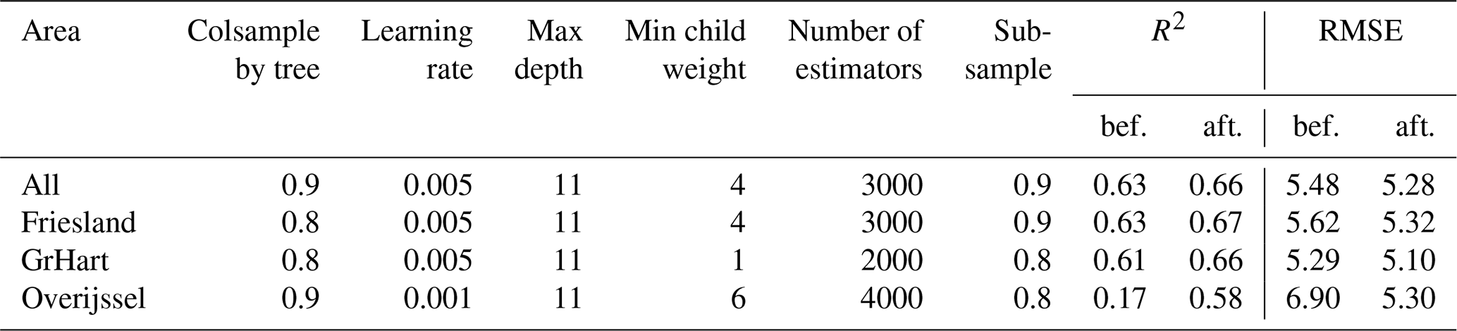
Figure 5 shows how the models trained on different areas perform when tested on another area. Although the Friesland model is the “best model” in terms of R² and bias, we see that the model based on all data performs better overall when applied on the test sets of individual areas. Generally, models trained on specific areas have worse scores when predicting for other regions. Simulating the Overijssel data by models from other areas (and vice versa: simulating the other areas with the Overijssel model) results in the lowest R² scores and the highest biases. For further analyses, we use the model based on all regions.

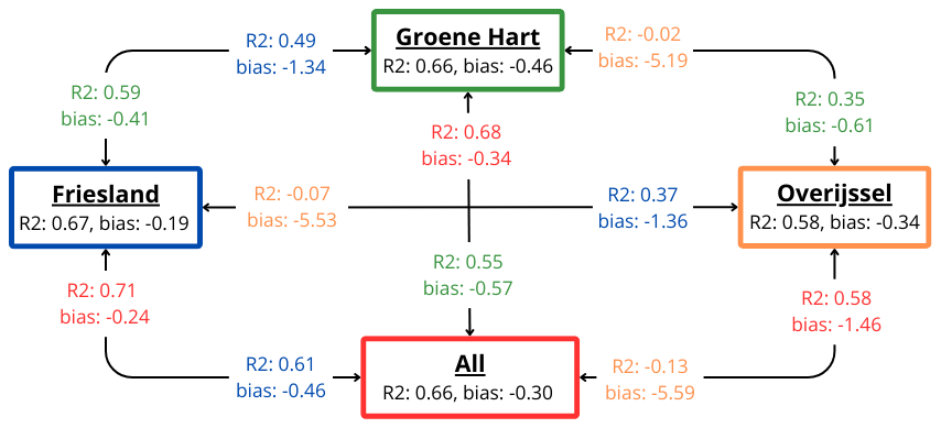
Figure 5 Machine learning models trained on data from different areas and corresponding performance scores when tested on the other areas. The same color is used for predictions from the same model. Here, the same features are used: PAR, T_sfc, RH, EVI, PeatDepth, and WTDe. The optimized hyperparameters are shown in Table 3.

3.2 Environmental response functions for CO₂ flux identified by Shapley analysis

To check the physical consistency of the trained model against prior knowledge and to understand how the model operates we analyze Shapley values for each of the selected features. Figure 6 shows an overview of all Shapley values for the model of all areas. A positive SHAP value indicates that the feature value has a positive contribution to the flux, i.e., increasing emissions or decreasing uptake, and a negative Shapley value indicates the opposite. Increasing PAR and EVI drive more uptake and/or less emissions, whereas increasing temperature and deeper water table depth have the opposite effect. The influence of RH and PeatDepth is not immediately clear from this bee-swarm plot.

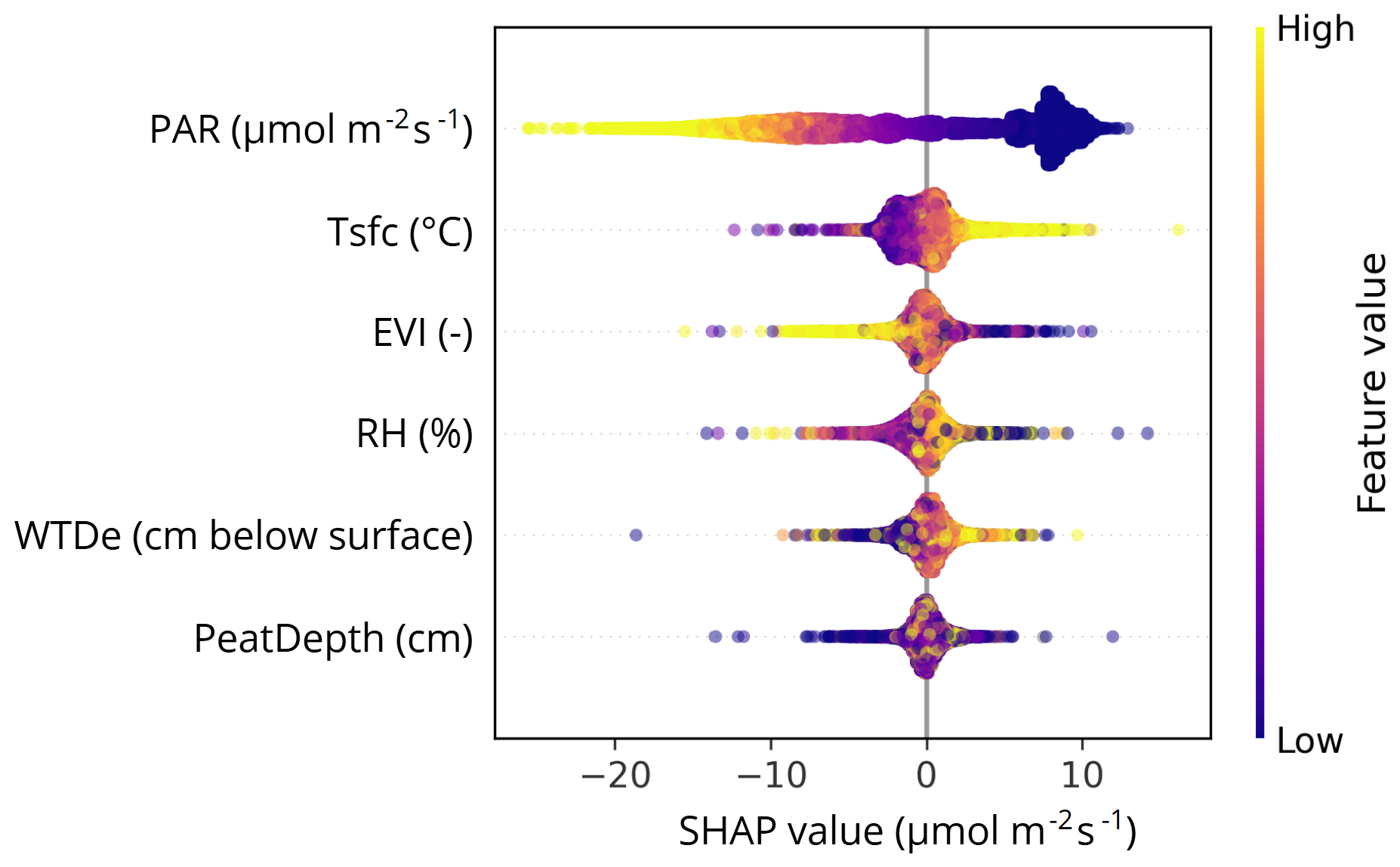
Figure 6 SHAP values for all features in the final model, representing the individual contribution of each feature to the final model outcome, depending on the value of that feature. The thickness indicates the number of data points. For example, there are many data points with low PAR and positive SHAP values, indicating that the model assigns a positive contribution to predicted CO₂ flux under low-light (i.e., nighttime) conditions. Abbreviations: PAR (photosynthetically active radiation), T_sfc (surface temperature), EVI (enhanced vegetation index), RH (relative humidity), and WTDe (effective water table depth).

We delve further into the Shapley values for the features through scatterplots shown in Fig. 7. Figure 7a shows the SHAP values of PAR and reflects the well-known light response curve, as learned by the model. As PAR increases, the contribution to the predicted flux becomes more negative, especially at higher temperatures. Conversely, with low PAR, SHAP values are positive and higher temperatures cause the flux to increase in the positive direction. Surface temperature drives nocturnal emissions (when PAR is 0) and drives daytime emissions once above about 15 °C. Optimal conditions for uptake are at RH between 40 % and 80 %, whereas drier conditions, correlating with the highest PAR values, drive emissions, as well as wetter conditions that correlate with nighttimes. As WTDe increases (i.e., becomes deeper) so does its SHAP value, but at deeper water levels this seems to level off or even reverse. Below, we examine this in more detail. EVI values above about 0.55 have a clear stimulating effect on CO₂ uptake and more so with higher PAR. EVI < 0.55 does not influence CO₂ exchange, especially with PAR = 0, indicating no clear effect of vegetation on nighttime emissions. This hints at emissions being driven mostly by heterotrophic respiration. Finally, peat depth shows no apparent relation with CO₂ exchange, even though its importance is high enough to be selected for the final model.

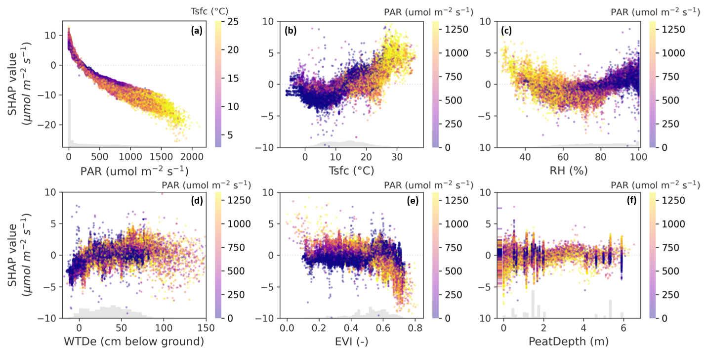
Figure 7 SHAP values of (a) PAR, (b) T_sfc, (c) RH, (d) WTDe, (e) EVI, and (f) PeatDepth (for abbreviations, see text or Fig. 6). The plots are colored by the values of another feature (T_sfc) in (a) and PAR in (b)–(f), which in some cases correlates with the depicted one due to diurnal or seasonal covariance. Nonetheless, the SHAP values represent the effect of only the selected feature on the x axis. The color gives insight on the conditions in which this effect is happening. The vertical lines in panel (f) originate from the towers, as a static peat depth map was used. The amount of scatter indicates the robustness of the found relationships.

As we are specifically interested in WTDe, Fig. 8 shows fitted linear, parabolic, and Gompertz lines on the bootstrapped Shapley values for WTDe. We tried fitting several other functions: bell-shaped functions, including and excluding a plateau in the middle; piecewise functions; sigmoid; logistic; Shepherd; and more, but the three depicted performed best on our data, where WTDe ranges from −0.2 to 1.5 m. The linear regression stops at the peak of the parabola at WTDe of 0.8 m. Similarly, the Gompertz function seems to truly flatten at this depth. However, the characteristic horizontal part at the beginning of the Gompertz curve is not visible in our data. Despite having different shapes, all three regression lines have approximately the same coefficient of determination (see Table 4). Up to 50 cm, the increase in emissions is coherent.

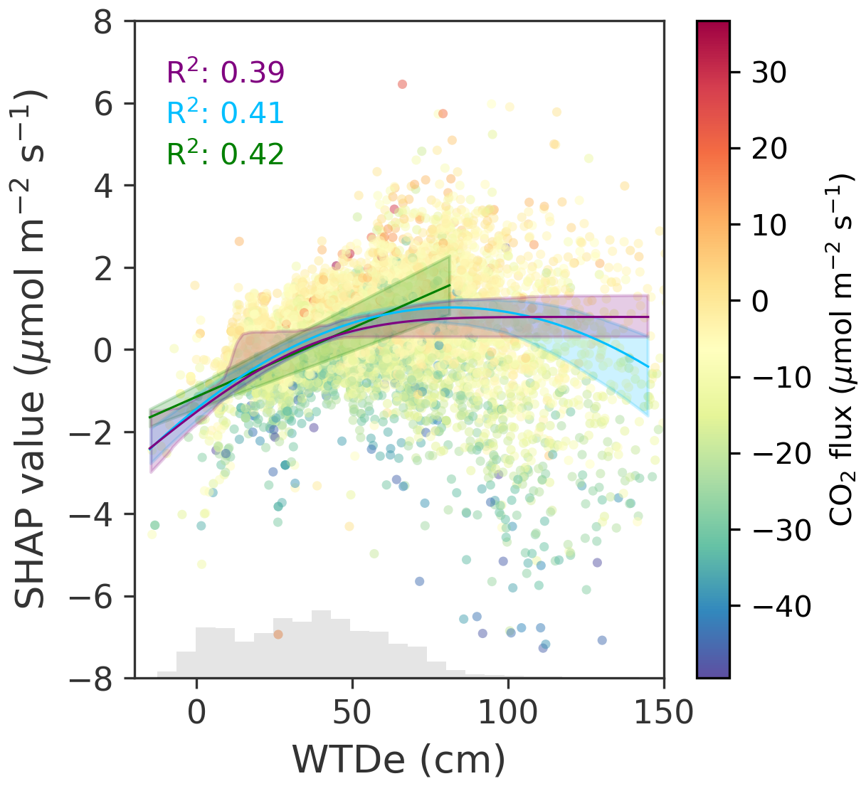
Figure 8 SHAP values with fitted linear, parabolic, and Gompertz functions, respectively colored green, light blue, and purple. The linear regression line stops at the peak of the parabola. The lines are drawn using the medians of 100 fitted parameters on the bootstrapped Shapley values. The shaded areas represent the 90 % confidence interval based on 5 % and 95 % of predictions at every WTDe value. The R² scores are the means of 100 regression lines. See Table 4 for the fitted parameters.

Table 4 Fitted parameters for the linear, parabolic, and Gompertz curves. The values represent the medians of the 100 fits based on bootstrapped models. The parameters in black correspond to CO₂ fluxes in µmol CO₂ m⁻² s⁻¹, whereas the parameters in gray correspond to fluxes in t CO₂ ha⁻¹ yr⁻¹. x is WTDe in centimeters. As the slope in t CO₂ ha⁻¹ yr⁻¹ is one of our primary results, we present its confidence interval here, 4.64 (3.95, 5.39) × 10⁻¹ per cm WTDe, while confidence intervals for all fitted parameters can be found in Appendix  E.

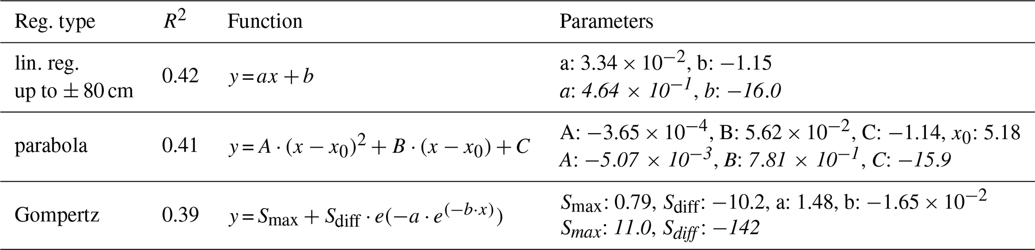
Italic: converted to t CO₂ ha⁻¹ yr⁻¹.

3.3 Simulated response of CO₂ fluxes to water table dynamics

For all our sites, we assembled half-hourly input data for 2020–2022. Inspecting the annual course of WTDe at the Overijssel sites, we found there is a systematic underestimation of the water table depth; i.e., OWASIS gives values associated with much drier conditions than the WTDe measurements. As a result, the average annual WTDe for Overijssel was the deepest of all our sites, while these sites are in wet nature areas. Hence, we discarded the simulations for the Overijssel sites. The WTDe at other sites was acceptable, although extremely deep summer water tables were often underestimated.

Letting the model predict the fluxes and calculating the annual balances for the sites in Friesland and the Groene Hart resulted in Fig. 9. For every site-year, there are three dots: one based on the actual WTDe values, one where we subtracted 10 cm, and one where we added 10 cm to every value of WTDe. Therefore, the triplets represent the sensitivity of the site's annual NEE balance to a 10 cm change in WTDe. The sensitivity varies from site to site, but for all sites combined, there is a curvilinear increase. Fitting a linear regression line yields a slope of 5.3 t CO₂ per ha⁻¹ yr⁻¹ per 10 cm WTDe below the surface. However, closer examination shows that the effect varies per site and per year and levels off at deeper water levels. We did not extend the simulated effects for deeper water table depths as those scenarios would become unrealistic without altering the other features.

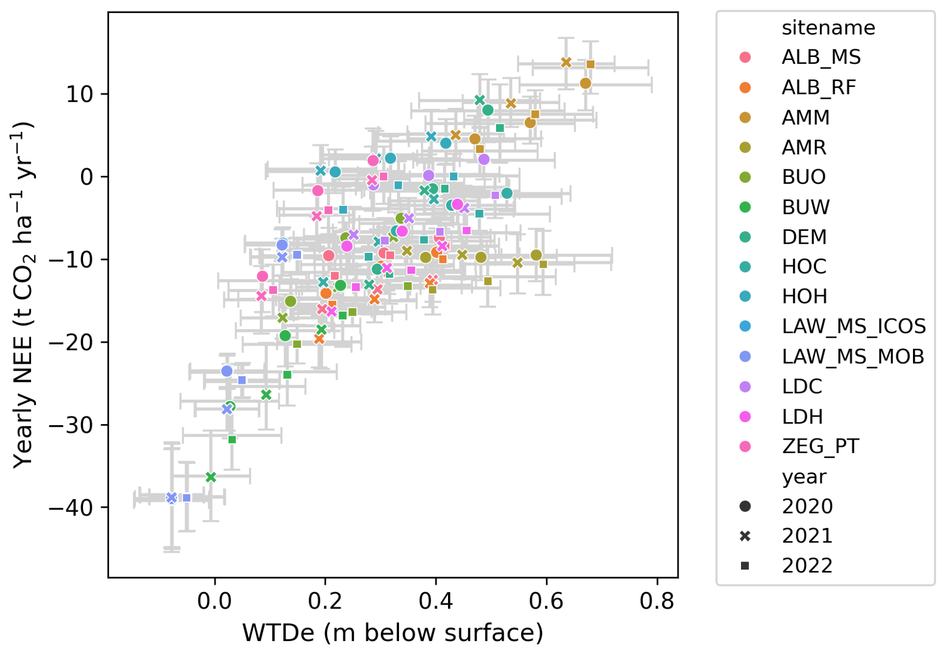
Figure 9 Simulated annual CO₂ balances for the sites in Friesland and the Groene Hart (see Fig. 2). The annual balances are sums of year-round predicted fluxes at 30 min temporal resolution using continuous input data from meteorological stations as well as static and dynamic maps. The triplets represent simulations for WTDe − 10 cm, actual WTDe, and WTDe + 10 cm. The uncertainty intervals represent standard deviations, where the vertical intervals are based on 100 annual balances based on the bootstrapped data and corresponding models. Fitting a linear regression line yields a slope of 5.3 t CO₂ per ha⁻¹ yr⁻¹ per 10 cm lowering of WTDe below the surface.

We grouped the sensitivity of predicted NEE fluxes to 10 cm WTDe increase by month, shown in Fig. 10. In gray, the range of sensitivity to 10 cm is depicted that is found in the literature. Although the mean of almost every month falls within the range and does not change sign, there is substantial scatter above and below. Furthermore, there is monthly variation in those means, being the lowest in summer and highest in winter months. We tested whether this variation is statistically significant with a Welch's t test, which accounts for the unequal variances across groups. Most month-to-month comparisons show significantly different means, but there is no distinct pattern (see Appendix F1). Grouping per season instead of per month shows that March–April–May (MAM) and June–July–August (JJA) do not differ significantly, but all other season comparisons do, suggesting different effects of 10 cm WTDe increase in autumn, winter, and spring/summer (see Appendices F2 and F3). If we compare sensitivities to raising WTDe by 10 cm (rewetting), all seasons are significantly different (Appendix F3). Additionally, there is a large variation between sites (see Appendix F4).

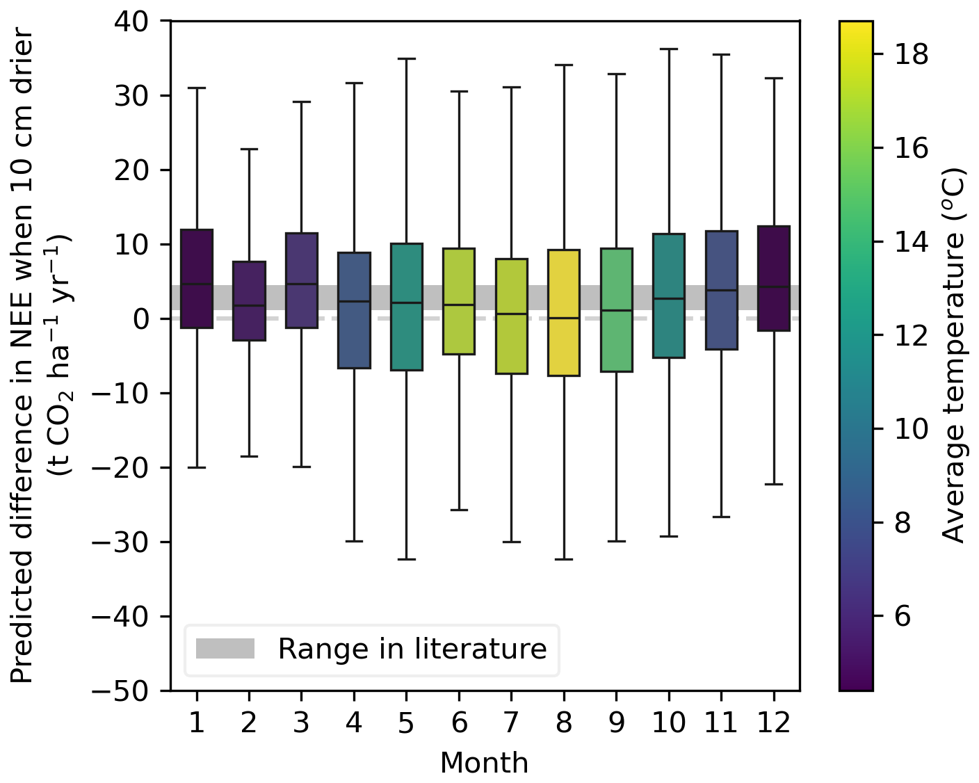
Figure 10 Monthly binned differences in NEE predictions when WTDe increased by 10 cm. The color represents the average temperature in our data for that specific month. The “range in literature” is based on the lowest and highest estimates of the groundwater–CO₂ slopes in the literature: 2.1 t CO₂ ha⁻¹ yr⁻¹ per 10 cm as found by Kruijt et al. (2022) and 4.5 t CO₂ ha⁻¹ yr⁻¹ per 10 cm as found by Fritz et al. (2017). See Fig. 11 and Appendix G for other estimates.

4 Discussion

4.1 Constructed models and their performance

Our final model explains 66 % of the observed variance and is able to provide further insights into key drivers of NEE. The found relationships with PAR, temperature, relative humidity, and EVI are in line with physically known processes. The effects of water table depth will be discussed in detail in Sect. 4.3,

The obtained R² seems acceptable given the complex interactions analyzed and random noise levels typical for eddy covariance observations. Compared to studies also modeling CO₂ fluxes but by traditional methods, this R² is in the same range (Jung et al., 2011; Zulueta et al., 2011; Dou et al., 2018). Similarly, Zhou et al. (2023), who combined satellite data and EC measurements with a random forest model, found an R² of 0.6. Still, the R² is not substantially higher than that of global models (e.g., Jung et al., 2020), despite the higher information density in our study. We attribute this to the relatively subtle variability within our study area, which encompasses seemingly similar systems in terms of land use, climate, and flux characteristics – making it more difficult to distinguish patterns than at the global scale. Other studies combining airborne and ground-based data using machine learning approaches tend to have higher R² (Metzger et al., 2013; Serafimovich et al., 2018; Vaughan et al., 2021), but these all focused on simulating heat fluxes, arguably a simpler process to analyze. Moreover, it appears that none of these studies used separate data subsets for learning and evaluation, as we did in the current study. Evaluating the model on the same dataset it was trained on would increase the R² for our best model from 0.66 to 0.89.

Although the Overijssel model performed acceptably, extrapolating to another area gives worse results than taking the mean of fluxes in the respective area (negative R² scores). This does not indicate that the Overijssel area itself is fundamentally distinct. Instead, it is a consequence of the WTDe data not reflecting the wet site conditions well. This might also explain why the All model performs better on GrHart and Friesland than when tested on its “own” test set, which includes Overijssel data, exhibiting the importance of accurate water table data. We trained a model on the combination of only the Friesland and GrHart data, and it obtained an R² of 0.67 and bias of −0.26: slightly better results than when the Overijssel data were included. We find that extrapolating between Friesland and GrHart gives reasonable results. Still, we find the best results when using the model trained on all data. Overall, we think that these machine learning models, especially the model including GrHart and Friesland data, perform adequately.

The models were able to find relationships with spatiotemporal variables, especially for key drivers like radiation, shown by little scatter in Fig. 7a. Additionally, other well-established processes such as the influence of temperature and relative humidity are well represented. Furthermore, the SHAP framework enables identification of processes affecting components of NEE that could otherwise not be distinguished. For example, at low PAR, emissions do not increase despite increasing EVI (up to EVI = 0.55), indicating emissions are mostly steered by heterotrophic respiration as opposed to autotrophic respiration. The increase in nighttime emissions for higher EVI values may indicate increased autotrophic respiration. Although additional research partitioning ecosystem respiration is required, these findings demonstrate the potential of SHAP and ML for process understanding.

While peat depth was important enough to be included in the final model, its SHAP values do not show a distinct effect. This is partly related to the static nature of peat depth and the large amount of data originating from towers, but it also suggests that peat depth, particularly when exceeding the typical range of water table fluctuations, has a minimal impact. Correspondingly, it has been suggested that peat depth exposed to air is a more direct indicator for peat decomposition and thus for CO₂ emissions than water table depth (Aben et al., 2024). In our study, we do not find this. The same holds for air-filled pore space, although this property is arguably more complex to model because of peat swelling and shrinking and varying porosity. However, it should be noted that the differences in performance when water table depth is replaced with another water-related feature are minimal, indicating a robust underlying process or relationship that the model is able to find.

We assumed our method of partitioning the data – selecting flight legs and weeks of measurements for the testing set and using the rest for training – avoided data leakage. To further examine this, we also applied two other partitioning strategies: one more stringent, selecting entire flights and sites for the test set, and one less stringent, selecting a random 20 % as the test set. The former resulted in worse models, but this depended on which sites were left out, as some provide more data and insights than others. Nonetheless, this partitioning strategy should be further examined in future research because it may better reduce data leakage. The models based on randomly selected training data all performed slightly better than the models we use in this study, indicating that our current strategy avoids some data leakage.

In the final optimized hyperparameters, we see that models differ mostly in minimum child weight. Models with a high value for this parameter are more conservative and end up with fewer splits. We believe the final model based on all areas achieves a good balance between capturing complex patterns and avoiding overfitting. Notably, only the Overijssel model was strongly improved by hyperparameter tuning. We hypothesize that the low initial performance scores are a result of the smaller dataset size and lower data quality. By increasing the model complexity (by lowering the learning rate and increasing the number of estimators), the model was able to identify relationships nonetheless. However, when attempting to generalize to other areas, it became clear the model was overfitting.

4.2 Combining airborne and tower data: pros and cons

Airborne and tower flux data are subject to different errors and uncertainties, intrinsic to their configuration and processing. One of these is flux divergence. Tower data observed only a few meters above a (grassy) surface represent true surface fluxes and any marginal divergence effects are largely corrected through a storage flux correction (Finnigan, 2006). For aircraft fluxes this is less trivial. We aim to minimize divergence errors by flying nominally at 200 ft (60 m) above the surface. This may be considered to be in the “constant flux layer” given that over all flights the average boundary layer height according to ERA5 reanalysis was 870 m at the time of the flights. Few studies have explicitly addressed CO₂ flux divergence: de Arellano et al. (2004) (Cabauw, in the Groene Hart area studied here), Casso-Torralba et al. (2008) (Cabauw again), and Vellinga et al. (2010) (Supplement, SW France). Apart from observational constraints to quantify it, CO₂ flux divergence is not unidirectional like sensible heat divergence. The entrainment flux for CO₂ can be significant in early morning and may change sign in the course of the day due to CO₂ release at night and uptake during the day. Such complications prohibit assessments of CO₂ flux divergence without dedicated observation strategies, let alone allow simple corrections. Neglecting advection, flux divergence equals the scalar storage term, i.e., temporal change in CO₂ concentration. From our tower observations we know these to be small around midday. For all these reasons, with Vellinga et al. (2010) and, e.g., Meesters et al. (2012), we assume CO₂ flux divergence errors are arguably smaller than other errors and not of constant sign (so they partially cancel out), and therefore they are neglected here.

As discussed, airborne and tower data have different qualities: airborne data are spatially exhaustive but temporally limited, and tower data are temporally continuous but with a limited spatial extent. On a given day, the airborne data provide a gradient of seasonally varying landscape features (e.g., WTDe and EVI), as opposed to point values at towers, and represent the entire area, making the input data more diverse. Because of their complementarity, we were able to develop an ML model that includes information on the daily cycle and extends beyond the tower locations. Nevertheless, practicalities when combining tower and airborne data may lead to some spurious correlations between features and targets due to two specific aspects. Firstly, tower data include nighttime measurements, while airborne data are only collected during the day, resulting in differences for weather-related features (PAR, RH, T_sfc) and almost all positive CO₂ fluxes stemming from tower data. Secondly, land use and soil classes are fixed for the tower data and variable for the aircraft data. Together, this led us to omit features from merged models that had distributions that were too distinct in airborne and tower data, such as the soil class “hV” (thin peaty earthy peat soils of > 120 cm deep). Although we prevented artifacts by excluding these features, we also omitted possibly valuable information. We created a categorical variable with the most prevalent land use or soil class in the footprint, but this did not improve model performance. Hence, our results underpin what has been previously found: the relationship with WTDe holds regardless of the land use or soil class (Evans et al., 2021; Tiemeyer et al., 2020).

Another significant difference between the airborne and tower datasets in our study is their size: the former has 10 400 records, the latter 66 400. Consequently, the merged dataset consists mainly of tower measurements, and if we construct a model only based on tower data, we see very similar performance of the two models. In a preliminary, unpublished study we conducted using only the Groene Hart data, the addition of airborne data significantly improved the ML model (R² increased from 0.47 to 0.61). However, in that case we had restricted datasets available: 7900 records for the tower data, originating from only two towers and spanning 6 months, and 2600 records for the airborne data (spanning 18 months). Under similar circumstances, when the tower dataset lacks spatial and temporal coverage, we believe the inclusion of airborne data can improve the model substantially. This was also demonstrated by Metzger et al. (2021), who showed that airborne measurements in combination with pre-field simulation experiments doubled the potential of a surface–atmosphere study. However, in the current study, as the tower network had been seriously extended, resulting in much higher spatial coverage, this was not directly visible in an improved R². We examined the airborne data's added value in three ways.

First, we tested excluding several towers from the training process to determine if we could replicate the added value of airborne data as in the previous study, and we compared resulting tower and merged models. The outcomes were highly variable because each tower has different qualities, lengths of measurements, presence of gaps, etc., but removal of certain towers showed similar results as in our previous study. Second, we trained one model with an equal number of airborne and tower instances, which resulted in an R² of 0.62. Training the model only on airborne data, on the other hand, resulted in an R² of 0.37. This suggests that it is not only the high amount of data that is beneficial for the model but that there is also intrinsic value in adding tower measurements to airborne data. Third, we let all models predict for airborne, tower, and merged datasets. The difference between the merged and tower model is shown when they are tested on the airborne data: the variance in airborne data was explained 34 % and 10 % by the merged and tower models, respectively. The airborne data represent regional fluxes originating from across the entire area. Hence, to model these regional fluxes, extending beyond the locations of the measurement sites, it is necessary to include airborne measurements in the model. Future research could investigate where the trade-off is: when do airborne measurements provide significant complementary benefits to tower data? With x number of towers of time y, how many flights should be done to obtain enough information? The costs of tower and airborne maintenance should be included. This research could shed light on the most efficient measurement strategies in areas with limited access to resources or with inaccessible terrains.

4.3 Influence of water table depth

4.3.1 Found relationship compared to previous estimates

Here, we compare our findings to groundwater–CO₂ emission relations found by previous studies, shown in Fig. 11 (parameters can be found in Appendix G). Note that although the literature relations, SHAP results, and site simulations share the same units (t CO₂ ha⁻¹ yr⁻¹), they represent different types of results. Regression lines of Boonman et al. (2022), Aben et al. (2024), Kruijt et al. (2022), and Evans et al. (2021) are based on NECB estimates and thus include corrections for annual carbon import and export through manure and harvest. In addition, they investigate different locations, partly use different measurement methods (chamber or tower), and are based on multi-site comparisons, thus indicating mostly spatial dependencies. The regressions based on SHAP values do not distinguish between temporal or spatial influence and depict the effect of changing WTDe on NEE flux as understood by the model, rather than actual CO₂ budgets. The annual NEE estimates, on the other hand, represent the sum of year-round simulated CO₂ fluxes with varying WTDe, neglecting carbon import and export as they are not part of the ML model.

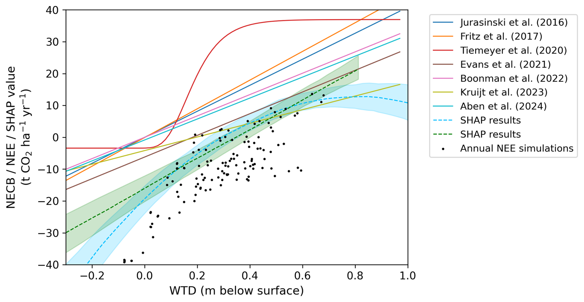
Figure 11 Comparison between current findings and literature studies on CO₂ flux vs. water table depth. Three types of results are shown. Regression lines from the literature based on annual NEE or NECB estimates. The dashed lines represent the linear and parabolic fits on the SHAP values. The simulated annual NEE totals are visualized in black for three situations per site (WTDe − 10 cm, actual WTDe, and WTDe + 10 cm). The shaded areas represent the 90 % confidence intervals of the SHAP regressions based on 5 % and 95 % of predictions at every WTDe value using the bootstrapped models. SHAP regressions are based on direct WTDe values, whereas literature studies and site simulations use annual averages. All fitted regressions can be found in Appendix G.

Both our NEE estimates and SHAP regression lines show more negative values than those reported by other studies. Firstly, for the annual NEE estimates, this can be partially explained by the difference between NEE and NECB budgets. On highly productive grasslands the export of harvest can be significant, as for example shown by Kruijt et al. (2022) where both NEE and NECB are reported for the same pastures as in the current study. Generally, the carbon in harvested biomass is released back to the atmosphere within a year, mostly in nearby areas. However, these emissions are not measured by the EC towers, though the aircraft might measure them when flying over, e.g., barns. Furthermore, simulated fluxes are underestimated due to the negative model bias, which mounts up to 4.2 t CO₂ ha⁻¹ annually. This bias may partly result from the lack of data on mowing events: the model continues to predict uptake as usual after mowing, whereas in reality, uptake stops immediately after grass removal (see Appendix H). Secondly, for SHAP values, the reference population mostly determines where SHAP = 0, and hence the change in impact on the model (i.e., the slope) is more meaningful than the exact level of impact (i.e., the intercept).

Apart from the negative offset, we find very similar relations to current estimates: per 10 cm WTDe, emissions increase annually with 4.6 t CO₂ ha⁻¹ based on SHAP and 5.3 t CO₂ ha⁻¹ based on annual NEE estimates. Since the annual NEE estimates are primarily based on farms with distinctive water table management – likely not representative of the entire area – we argue that the SHAP slope, which is based on the full dataset, is a better estimate. Considering the different approaches used, clarifying the negative offset, the correspondence with the literature is remarkable. It suggests that the underlying WTD–CO₂ relation persists, also when harvest and manure are disregarded. This may be because we investigate the regional scale, where local fluctuations balance each other out. Another explanation might be that harvesting biomass has mostly short-term impacts on the system (see, e.g., Appendix H). With the combination of aircraft measurements, instantaneous data rather than annual totals, and machine learning, we were able to extract this fundamental groundwater–CO₂ emissions relationship.

4.3.2 Nonlinearity of the found relationship

We did not find a linear relationship over the entire range of WTDe in our data (see Figs. 8, 9, and 11). Emissions undoubtedly rise with deeper WTDe, but deeper than 0.8 m, they cease to increase. Based on the SHAP explanations, the optimum-based curve explains the data slightly better than the Gompertz curve, indicating a decrease rather than a stabilization of the effect at deeper water levels. We lack sufficient data at these deeper water levels to make a concluding statement, but given that our data points represent instantaneous NEE fluxes instead of annual estimates, it is entirely plausible that a curve with an optimum indeed better represents the underlying process. For example, in conditions with WTDe > 0.8 m, moisture conditions can be sub-optimal for peat decomposition. Nijman et al. (2024) and Campbell et al. (2021) found similar response curves comparing nighttime ecosystem respiration to water-filled pore space and volumetric soil moisture content, respectively. In these studies, as well as in the current study, instantaneous measurements are compared, as opposed to the studies discussed above. Furthermore, the relationship between WTDe and CO₂ flux with deeper water levels is less direct, since the actual soil moisture in the unsaturated zone can vary substantially, which potentially explains the larger scatter in Fig. 8 – in addition to fewer available training data.

As opposed to Tiemeyer et al. (2020), who find saturation around a WTDe of 0.4 m, we find the increase to persist until 0.8 m, as was also found by Boonman et al. (2022) and Aben et al. (2024) for average summer WTDe. In the study by Tiemeyer et al. (2020), the amount of data for water levels deeper than 0.4 m is limited. Because we include fluxes on a short timescale and we cover a wider range of WTDe values by using the aircraft, we have a larger dataset to support the observation of increasing emissions up to 0.8 m. Additionally, we do not find an initial plateau at shallow water levels, contrary to what is currently assumed. Although we included wet sites, such as those in Overijssel, the water information product we used was not able to capture these wet conditions and gave incorrect values. Hence, our model was not trained properly on wet sites, and we cannot substantiate the lack of a plateau.

4.3.3 Intra-annual and spatial variability

Based on the above discussion, our results are mostly in line with previous studies, with two notable exceptions: the optimum-based shape instead of the linear or Gompertz functions and the increase in emissions until 0.8 m instead of 0.4 m, also found by Boonman et al. (2022) and Aben et al. (2024). A third insight is the intra-annual variation of sensitivity to WTDe change, as shown in Fig. 10 and in Appendix F. Further drainage in summer might not impact emissions as much, whereas drainage in winter has a bigger impact. This might be a reflection of the monthly varying WTDe: in summer, with very deep groundwater levels, the available oxygen for decomposition does not linearly depend on the groundwater and is also determined by the soil structure and its capillary action. As a result, at very deep water levels, the soil in the unsaturated zone can be relatively wet and decrease the effect of further drainage. On the other hand, with more shallow water levels in winter, the presence of roots in the unsaturated zone leads to soil desiccation, promoting oxygen availability down to the water table. Hence, when the water table is lowered, this has a more direct effect on CO₂ emissions. Furthermore, we find that raising the WTDe by 10 cm has a significantly different effect across all seasons. Our methodology enables future research on intra-annual occurrences such as season-based mitigation measures and extreme weather events.

In the current study, we applied the simulations to the site locations, which show high variability in responses. These site simulations were partially motivated by the goal of comparing predictions to measurements, as in Appendix H. However, since our model is trained on data covering the entire region – enabled by the use of aircraft data – the simulations can be applied to any location in the area, which can be of interest to policy-makers. Although our input data are too coarse to predict the emissions at farm level, the model can provide insights at the municipal or provincial scale in carbon flux dynamics over the years.

4.4 Implications for mitigation strategies

Our findings suggest that to reduce CO₂ emissions, the optimal water management would be to set the water level as high as possible. To reduce greenhouse gas emissions in general and mitigate climate change, the trade-off with methane should be taken into account (Buzacott et al., 2024). The slope we found lies at the upper limit of current estimates, and our results show that emissions continue to increase down to a WTDe of 0.8 m below the surface, as opposed to 0.4 m in Tiemeyer et al. (2020). Together, these results suggest higher emissions than those that would otherwise be calculated based on previous studies. This would entail effective mitigation strategies being even more crucial, as the potential for carbon emissions from drained soils may have been underestimated. As such, mitigation measures should take into account not only average annual water table depth, but also the different system behavior throughout the year. Measures should focus on rewetting during the summer and specific attention should go to not lowering the water table during winter. However, the evaluation of potential mitigation measures did not fall within the scope of our study. As we did not incorporate data on mitigation efforts into the model, we cannot draw conclusions in that regard. Nevertheless, this study is part of the Netherlands Research Programme on Greenhouse Gas Dynamics in Peatlands and Organic Soils (NOBV) and contributes to the corresponding measuring, monitoring and modeling framework. Within this framework, the efficiency of mitigation measures is widely studied using both data-driven methods and process-based models such as SOMERS (Erkens et al., 2022), and findings will be reported to policy-makers.

4.5 Recommendations

4.5.1 Incorporation of additional data

A general remark on the findings in this study is that the water level data are from a company that develops and maintains the OWASIS information products together with water boards and knowledge institutes. Comparing OWASIS WTDe to measured WTDe at tower locations, we found that values in summer were often underestimated. Potential sources of errors in the OWASIS data are heterogeneous infiltration capacity within pixel cells or limitations of remote sensing in capturing deeper soil layers. Despite these uncertainties and underestimations, we consider the OWASIS product suitable for the purposes of this study, as it covers the entire study area, and we have a satisfactory amount of data to balance out pixel errors.

Still, future research should prioritize including a high-quality soil water product of high(er) spatial resolution. Due to the use of aircraft data, the information on water should be spatially distributed, and measurements at tower sites do not suffice. The Netherlands has manifold regional hydrological products that can be used for future regional studies (NHI, 2025). In addition, there are numerous remote sensing products that could be used or combined for water-related information, possibly including ground-truth data, as was done by Koch et al. (2023) for Denmark, who developed a WTD map for Danish peatlands with a spatial resolution of 10 m. Considering the likelihood that farmers might apply mitigation measures such as changing the water level management or adding a clay layer on the peat, corresponding data would be valuable for subsequent studies. Furthermore, a vegetation index with higher spatial and temporal resolution could be incorporated, such as from Sentinel satellites or from the Dutch groenmonitor.nl website, ideally enabling identification of mowing events. In the current study, we did not directly incorporate mowing or harvest events.

4.5.2 Methodological advancements

As mentioned previously, future research should investigate the optimal combination of tower and aircraft data. This way, strategies for the modeling of remote or data-sparse locations can be developed. Herein, a stricter train–test algorithm can be applied. For the tower footprints, we suggest taking a wind-direction-based average footprint in the future as opposed to a circular footprint. The SHAP framework has proven highly effective in revealing the processes understood by the ML model. By making the reference population more representative, the base value might become more meaningful. However, the SHAP values do not per definition reflect causal relationships. As an extension to the interpretation by SHAP, therefore, we recommend including more causality-based and/or physics-based components. Here, we discuss some promising approaches and our first attempts in applying them. However, they are subject to future plans.

To start, information theory (IT) has already been used in studies to examine causalities of CO₂ fluxes (Arora et al., 2019; Farahani and Goodwell, 2024; Yuan et al., 2022). It is a mathematical approach to study the amount of information in a dataset or process based on Shannon entropy: a measure of uncertainty in a system, quantifying its unpredictability. In the current study, Shannon entropy can shed light on the information in tower vs. airborne data. We computed the Shannon entropy of CO₂ fluxes in our tower, airborne, and merged datasets (tower + airborne), as well as an entropy-based metric based on Farahani and Goodwell (2024) (see Appendix I for the formula and results). The airborne data have the highest Shannon entropy, indicating the highest level of information in the dataset, followed by the merged data. The results on the metric suggest that the merged model captures the variability in the data better compared to the airborne or tower models. However, the differences are relatively small. Additionally, the results show that the tower model is overly complex or noisy, whereas the airborne and merged models slightly underrepresent the variability in the data, meaning they smooth over some of the finer details or variability in the CO₂ fluxes (Farahani and Goodwell, 2024). At the regional scale, we believe the latter is preferable.

A second option is to alter the loss function in a deep learning model, which is more modifiable than in XGBoost. For example, transfer entropy can be minimized through the loss as is done by Yuan et al. (2022), or directly physically inspired functions or models can be implemented, as successfully done by Liu et al. (2024). New, innovative approaches such as double ML based on causality offer great opportunities for further exploring the greenhouse gas dynamics in drained peatlands (Cohrs et al., 2024).

5 Conclusions

In this study, we applied boosted regression trees to learn the relationship between CO₂ flux and landscape characteristics from drained peatlands in the Netherlands. We investigated data from the three main fen meadow areas in the country (Groene Hart, Friesland, and Overijssel) and finally constructed a model based on all areas combined. We merged CO₂ flux data from both airborne and tower measurements, and, to our knowledge, this study is the first to use this combination of CO₂ data as input for a machine learning model. The models were optimized with feature selection and hyperparameter tuning, and we accounted for data leakage by splitting the training and testing set based on flight legs and week numbers. Subsequently, we used the SHAP framework and simulations to assess the influence of the most important and relevant environmental drivers.

The method works and the models perform reasonably well with R² scores between 0.58 and 0.67. We found that extrapolating the model from one region to another performs adequately as long as water table training data are accurate, but the model including all regions is best for this purpose. As long as the feature subset contained information on the daily and seasonal cycles, information about peat, and some water-related feature, the scores of the models were very similar. Hence, the final, robust features that explained most of the variance in CO₂ fluxes are PAR, temperature, relative humidity, EVI, peat depth, and effective water table depth (WTDe).

Based on the SHAP values, we find an increase in CO₂ emissions until a water table depth of around 0.8 m below the surface. These emissions increase by 4.6 t CO₂ ha⁻¹ yr⁻¹ per 10 cm WTDe on average (90 % confidence interval: 4.0–5.4 t CO₂ ha⁻¹ yr⁻¹), which is in agreement with other estimates, albeit at the higher end of the range found in the literature. Together, these results suggest higher emissions related to WTDe than previous studies. Furthermore, we find that an optimum-based function describes the influence of WTDe best within our WTDe range. However, further research using instantaneous measurements on a short timescale (thus including data at deeper water levels) should point out whether the emissions decrease or stabilize after 0.8 m. We find intra-annual and spatial variation in the response of CO₂ flux to 10 cm drying and rewetting. These aspects should be taken into account when developing mitigation measures.

Future research should prioritize including data on water table depth with higher spatial resolution that better capture wet and extremely drained conditions. Causality-based approaches and physics-guided ML models form a promising direction for future studies. A comprehensive comparative study on the synergies between airborne and tower data could contribute to establishing efficient, cost-effective measurement strategies. In conclusion, we have quantified the impact of groundwater changes on CO₂ fluxes across drained peatlands in the Netherlands, providing crucial understanding in support of the 1 Mton reduction target by the Dutch government.

Appendix A: Processing steps for airborne and tower flux calculation and filtering

(McDermitt et al., 2011)Papale et al., 2006Vickers and Mahrt (1997)(Foken et al., 2004)(Vellinga et al., 2013)

Table A1 Processing steps for tower and airborne flux calculation and filtering. EddyPro was used for tower fluxes.

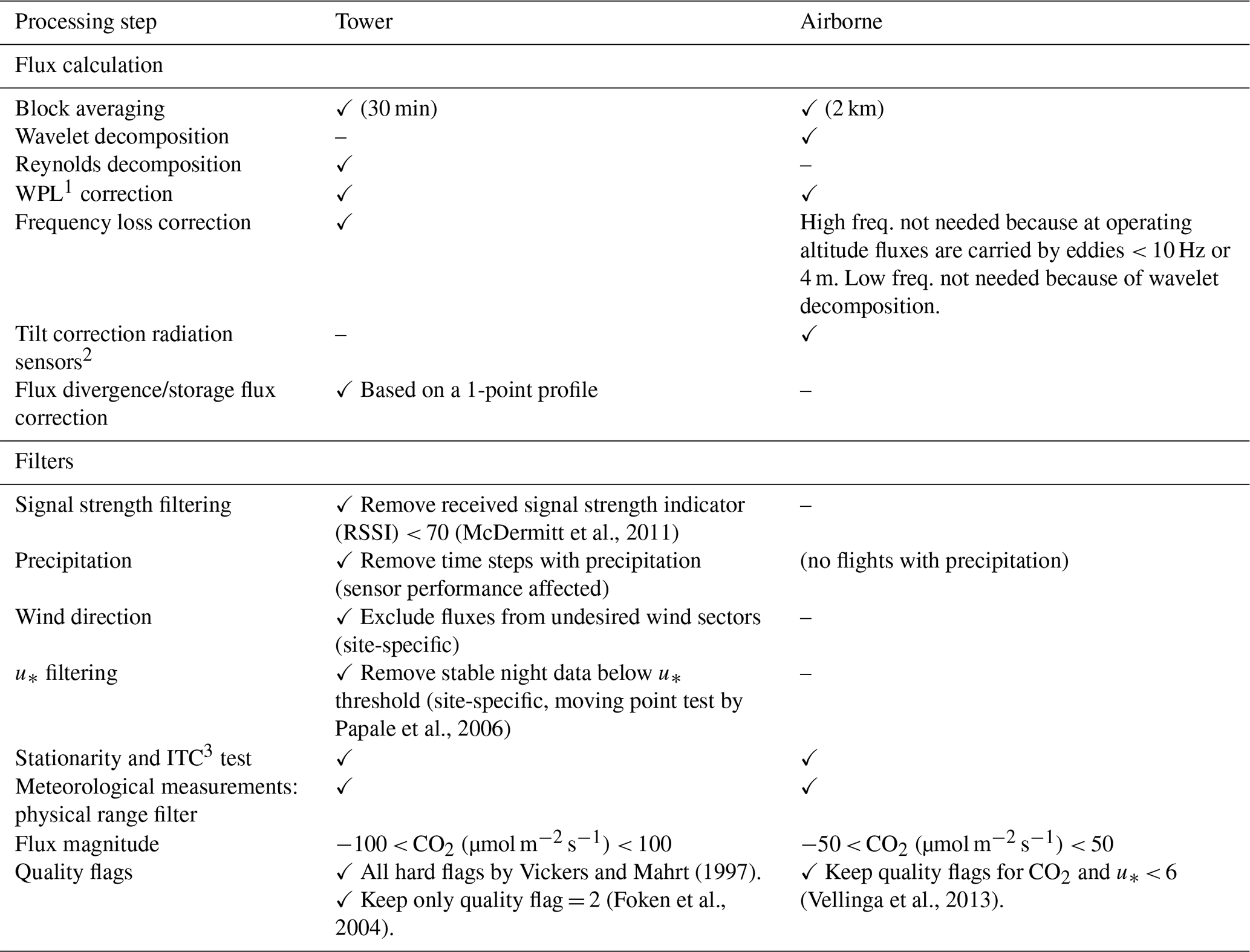
¹ Webb, Pearman, and Leuning (Webb et al., 1980). ² Based on aircraft attitude and solar position. ³ Integral turbulence characteristics.

Appendix B: Reclassification tables

B1 Reclassification of land use classes

Table B1 Reclassification of land use classes.

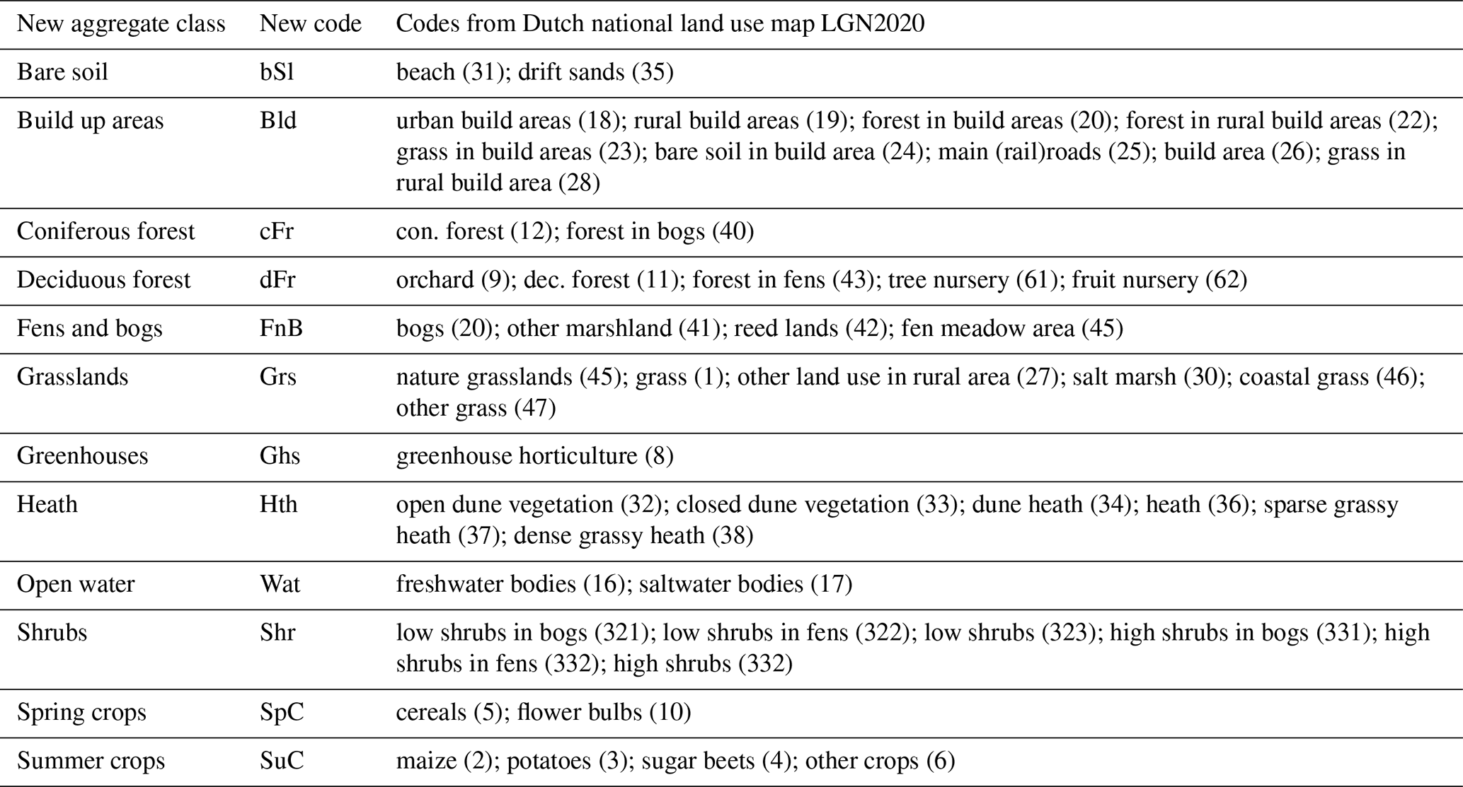
B2 Reclassification of soil classes

Table B2 Reclassification of BOFEK2020 soil classes into new aggregate classes for mineral soils.

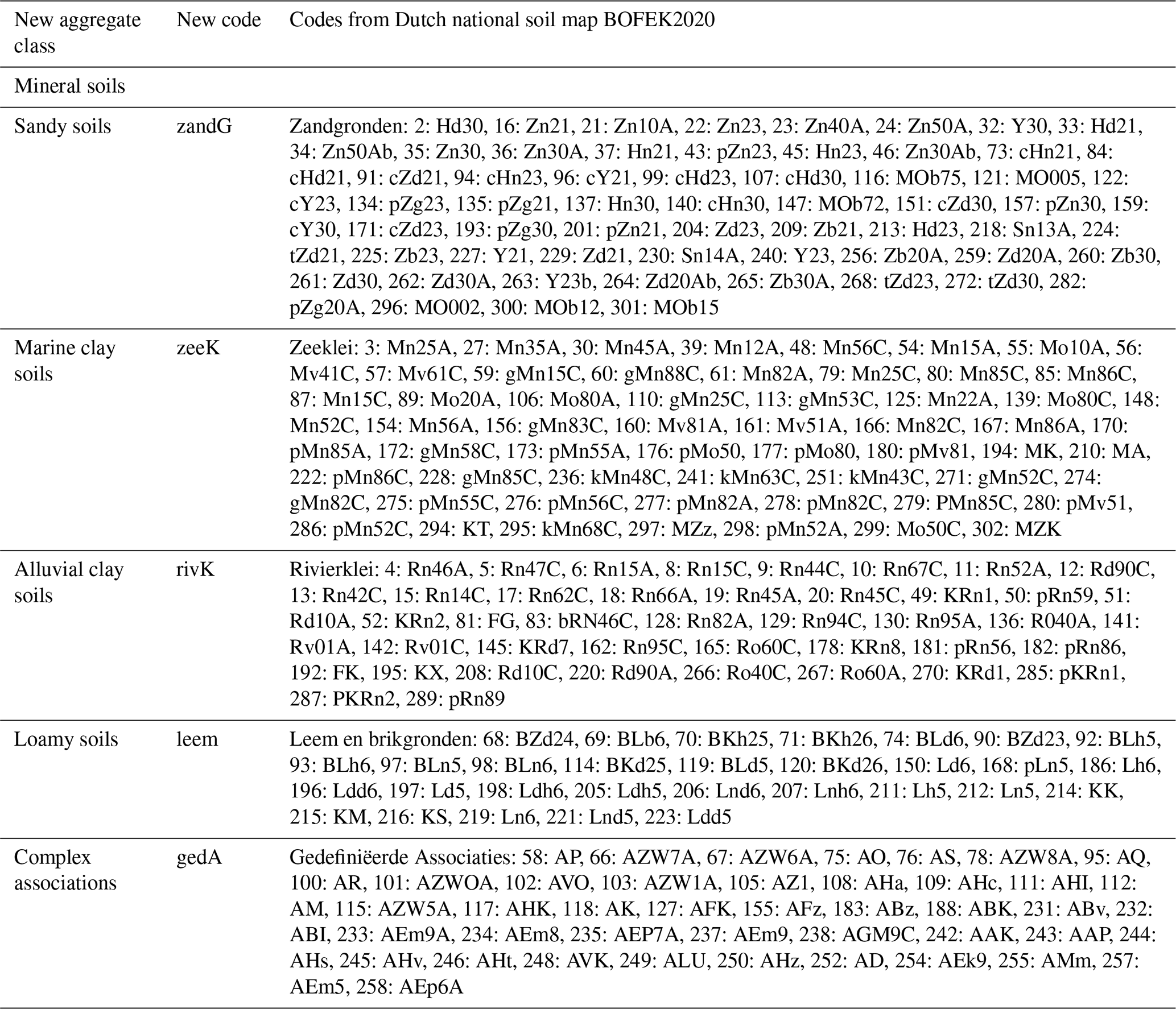
Table B3 Reclassification of BOFEK2020 soil classes into new aggregate classes for organic soils.

Appendix C: Hyperparameter tuning grid

Table C1 Parameter grid for hyperparameter tuning.

Appendix D: Model optimization results

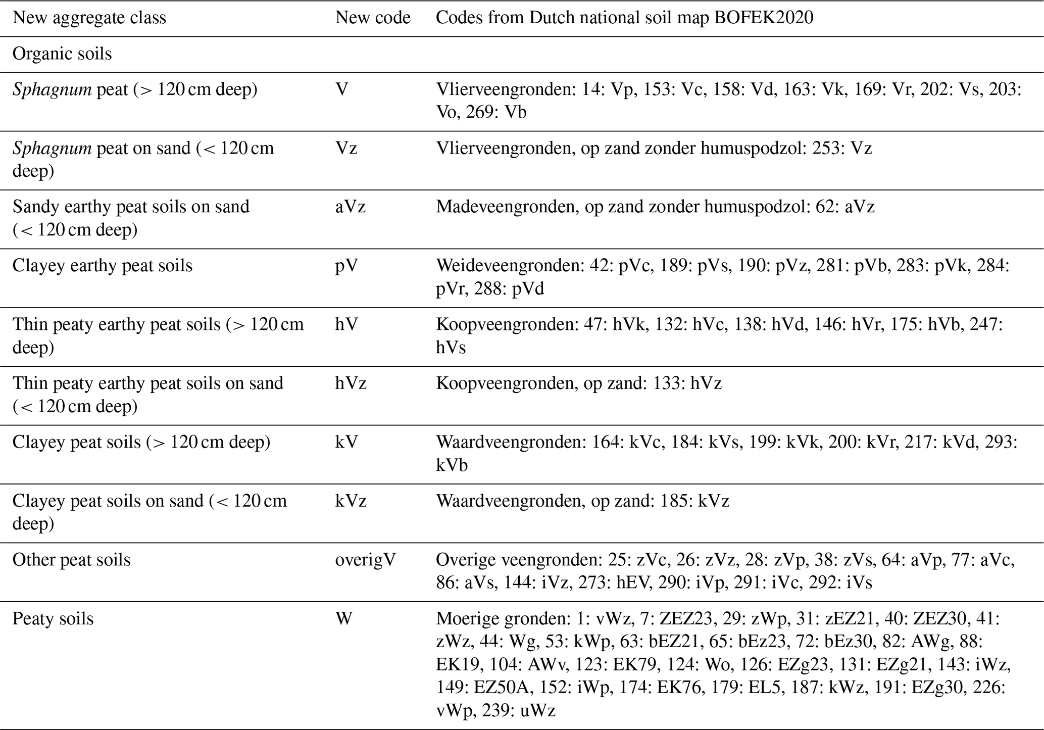
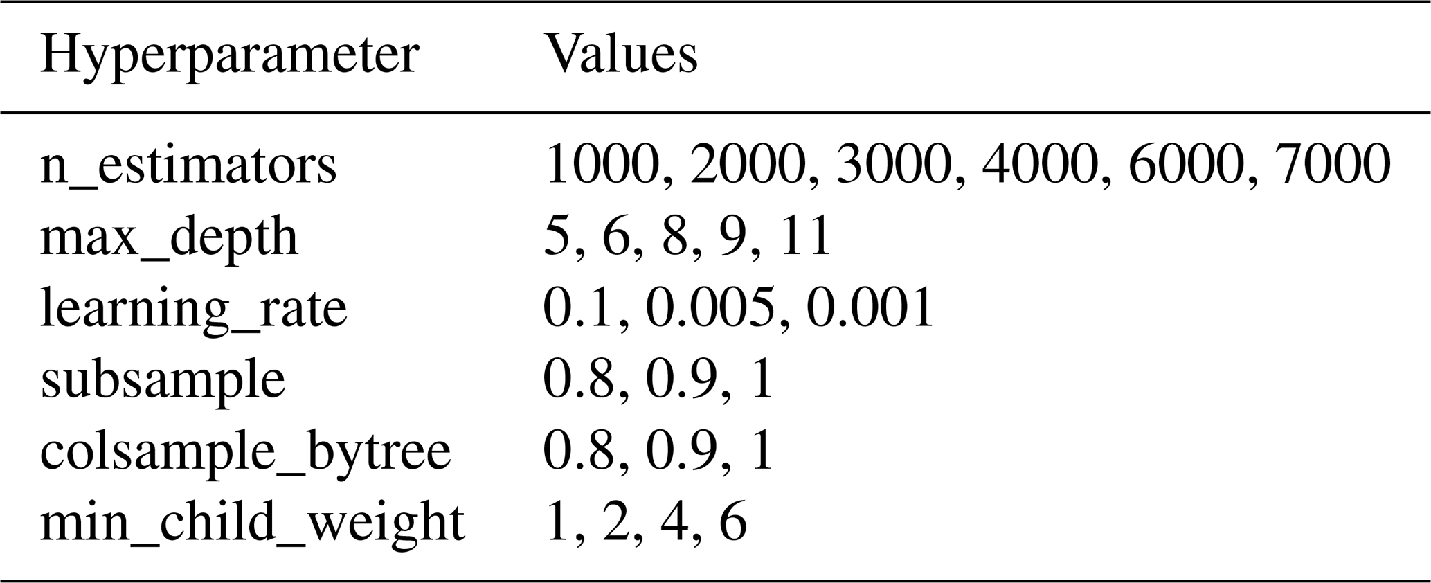
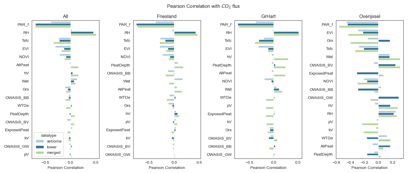
Figure D1 Pearson correlation between a selection of features and CO₂ flux for airborne, tower, and merged datasets per area. The selected features are the most correlated throughout all datasets. The other features (for example, other soil classes and land use classes) are not shown here for simplicity of the figure. Abbreviations of features are as follows. PAR_f: photosynthetic active radiation, RH: relative humidity, T_sfc: surface temperature, EVI: enhanced vegetation index, NDVI: normalized difference vegetation index, AllPeat: percentage of footprint in peat classes, hV: percentage of footprint in soil class thin peaty earthy peat soils (> 120 cm deep), pV: percentage of footprint in soil class clayey earthy peat soils, kV: soil class clayey peat soils (> 120 cm deep), Wat: percentage of footprint in land use class open water, Grs: percentage of footprint in land use class grasslands, OWASIS_BB: available open pore space from OWASIS, OWASIS_BV: soil moisture from OWASIS, OWASIS_GW: groundwater level from OWASIS (mbs), WTDe: effective water table depth, ExposedPeat: peat depth exposed to air.

Appendix E: Confidence intervals of SHAP regression lines

Table E1 Fitted parameters on the SHAP regression lines: LR indicates linear regression, P indicates parabola, and G indicates Gompertz. The formulas are shown in Table 4. Values in parentheses indicate 90 % confidence intervals, based on the 5th and 95th percentile of all bootstrapped regression lines.

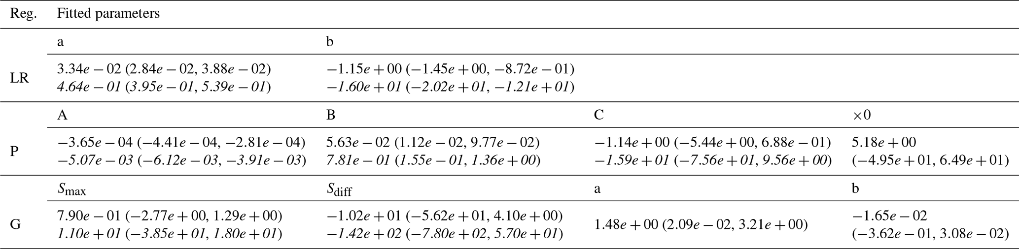
Italic: converted to t CO₂ ha⁻¹ yr⁻¹.

Appendix F: Sensitivity of NEE when WTDe ± 10 cm

F1 Welch's t test on monthly values

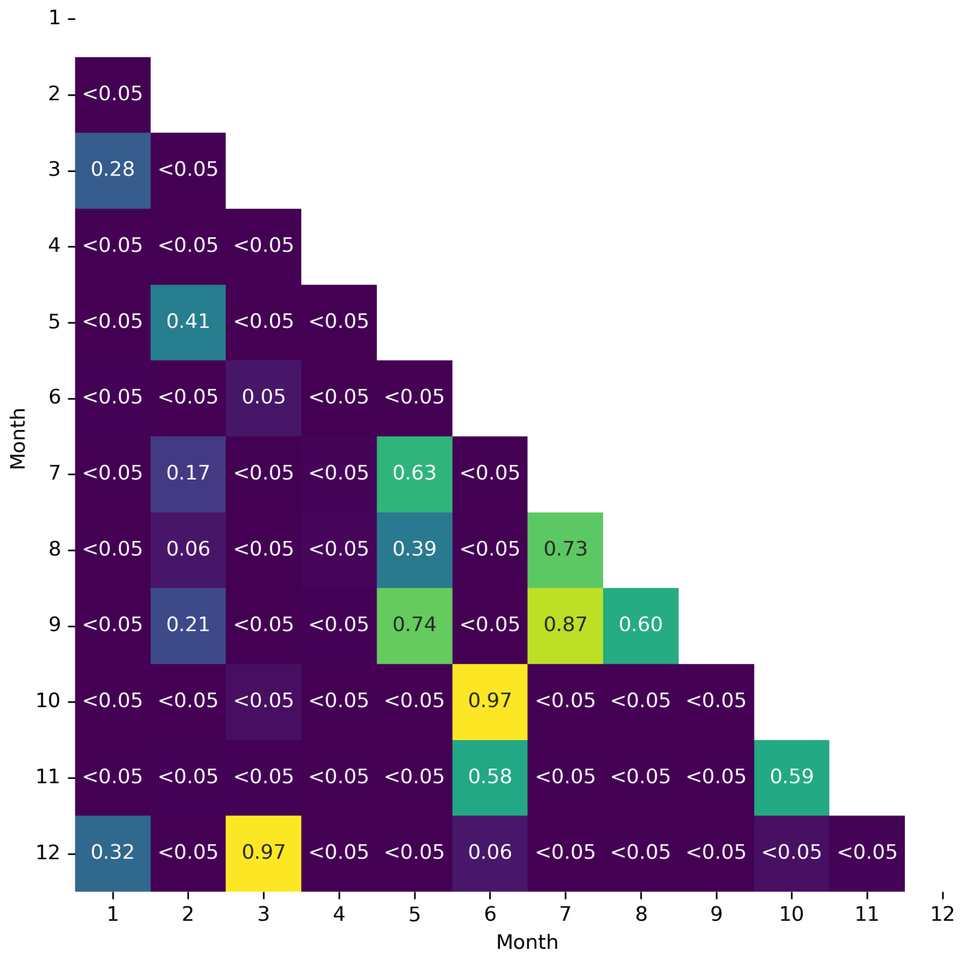
Figure F1 Results of p values for month-to-month comparison of responses to 10 cm drying in WTDe using Welch's t test.

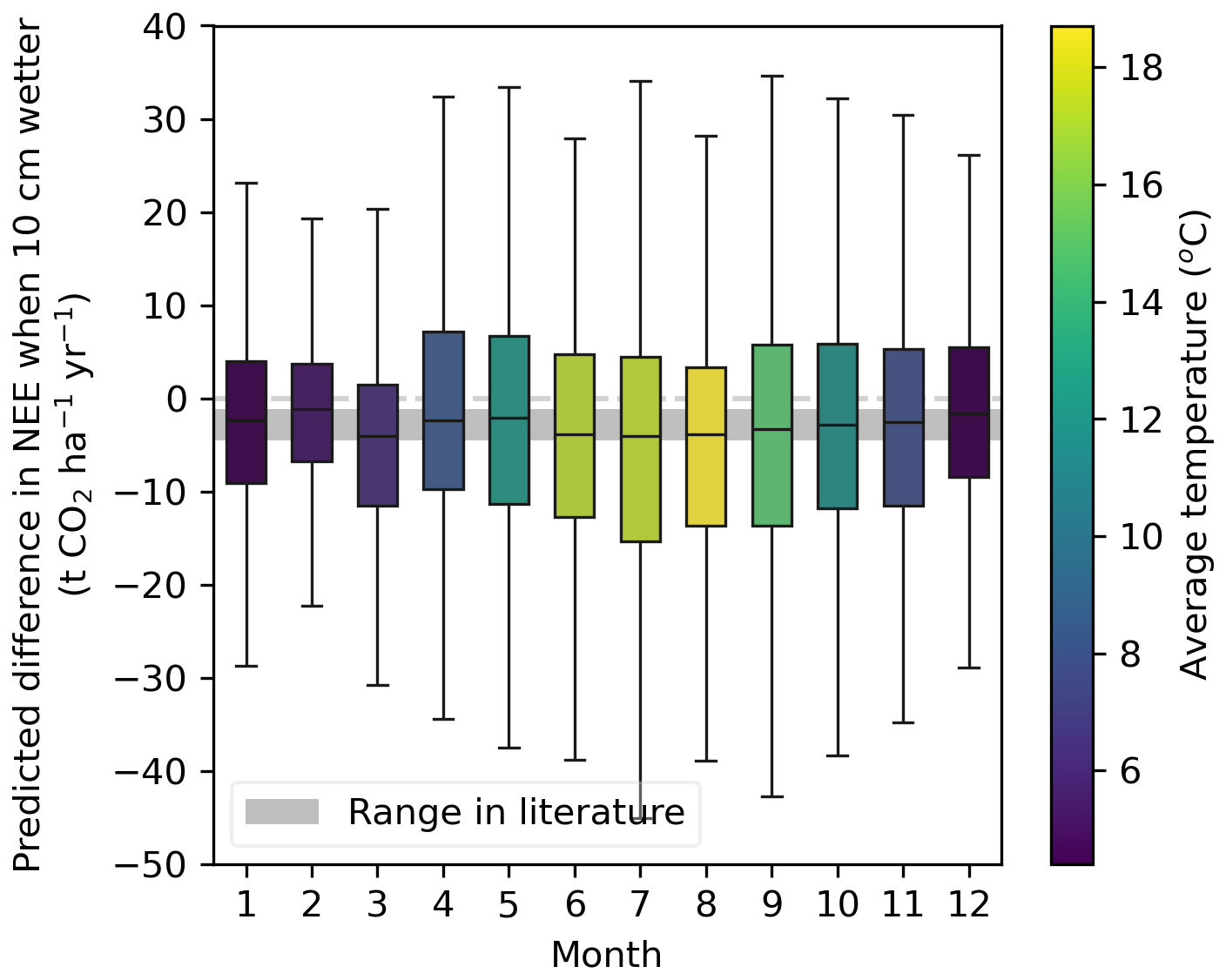
Figure F2 Monthly binned differences in NEE predictions when WTDe was raised by 10 cm. The color represents the average temperature in our data for that specific month.

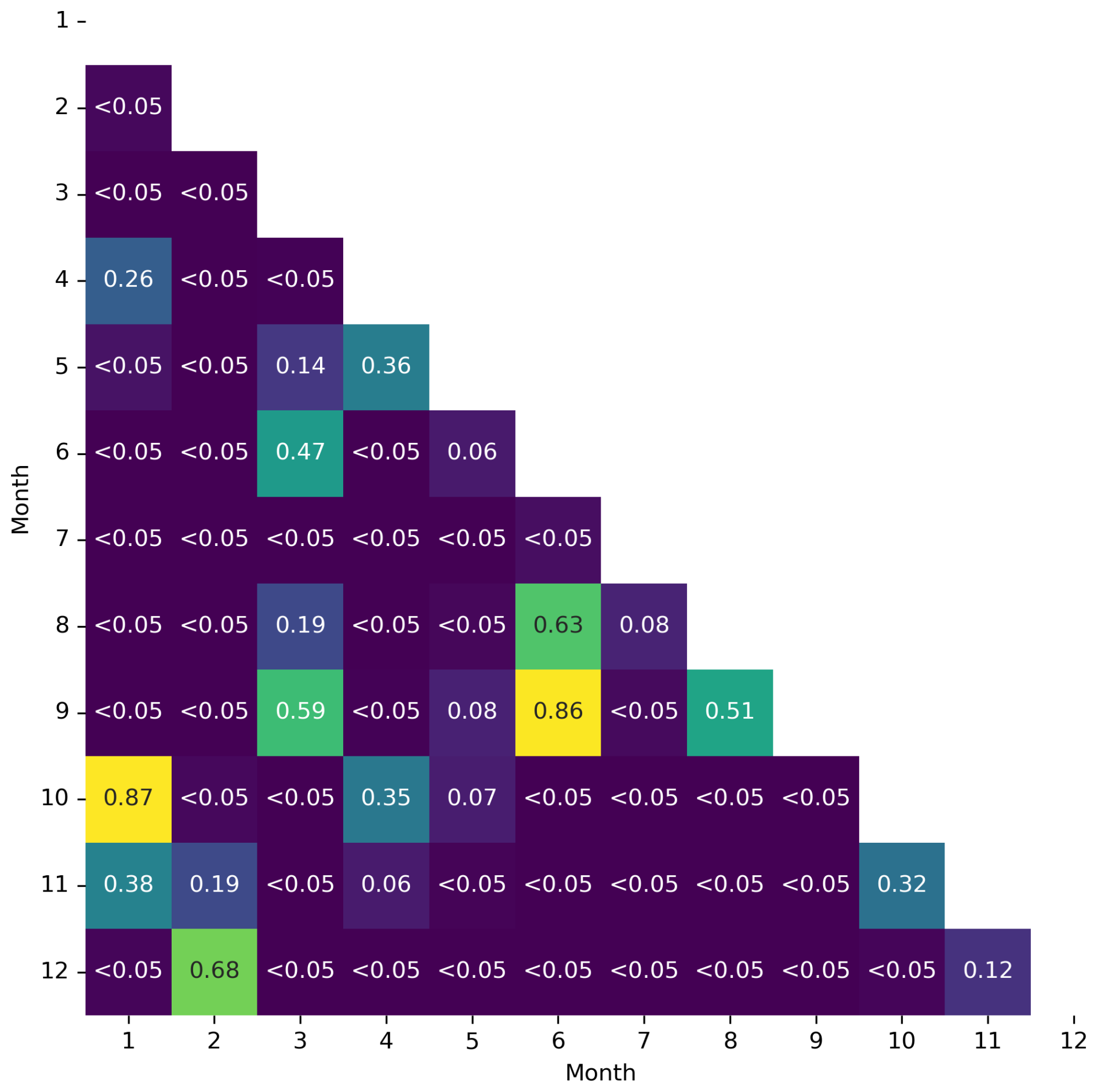
Figure F3 Results of p values for month-to-month comparison of responses to 10 cm rewetting in WTDe using Welch's t test.

F2 Seasonal difference in fluxes after change in WTDe

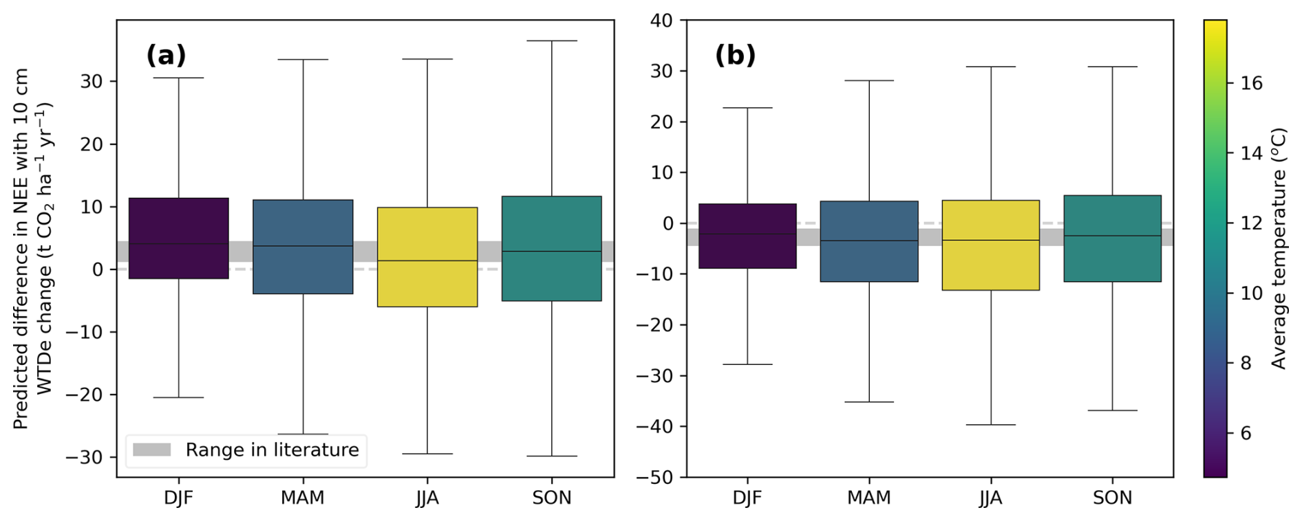
Figure F4 Responses of lowering of WTDe by 10 cm for all sites combined, binned per season. Panel (a) shows the results for 10 cm drier and panel (b) shows 10 cm wetter. Note the different y axes.

F3 Welch's t test on seasonal values

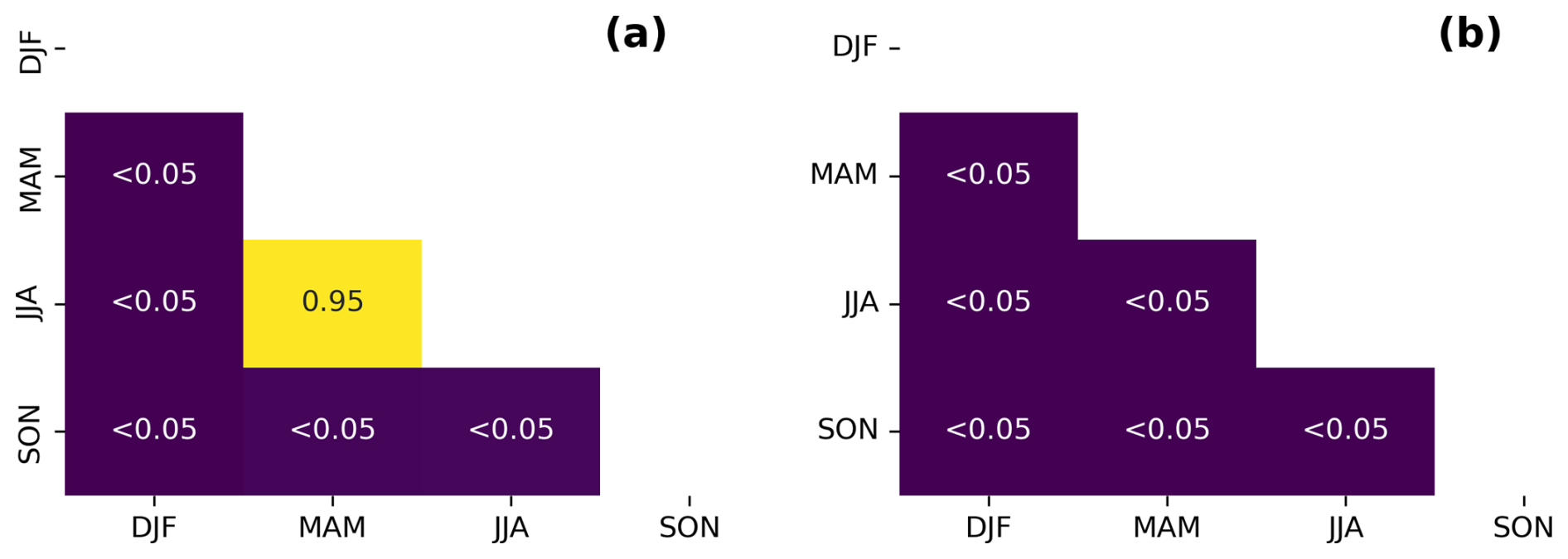
Figure F5 Results of p values for season-to-season comparison of responses to 10 cm change in WTDe using Welch's t test. Panel (a) shows the results for 10 cm drier and panel (b) shows 10 cm wetter.

F4 Sensitivity per site

Figure F6 Responses of sites to lowering of WTDe by 10 cm, binned per season.

Figure F7 Responses of sites to raising of WTDe by 10 cm, binned per season.

Appendix G: Relationships found in the literature

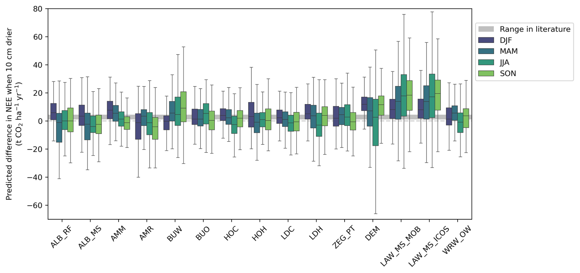
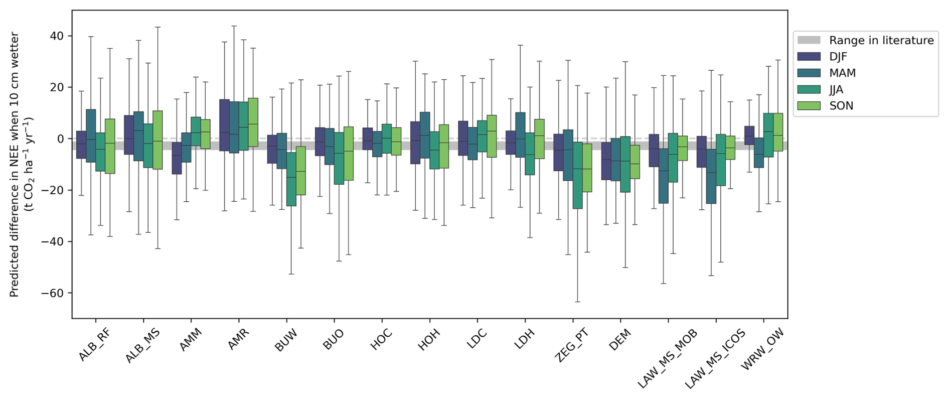
Table G1 Literature studies and corresponding found relationships between emissions in tons of CO₂ ha⁻¹ yr⁻¹ and water table depth below the surface level in meters.

Appendix H: Model predictions and mowing events

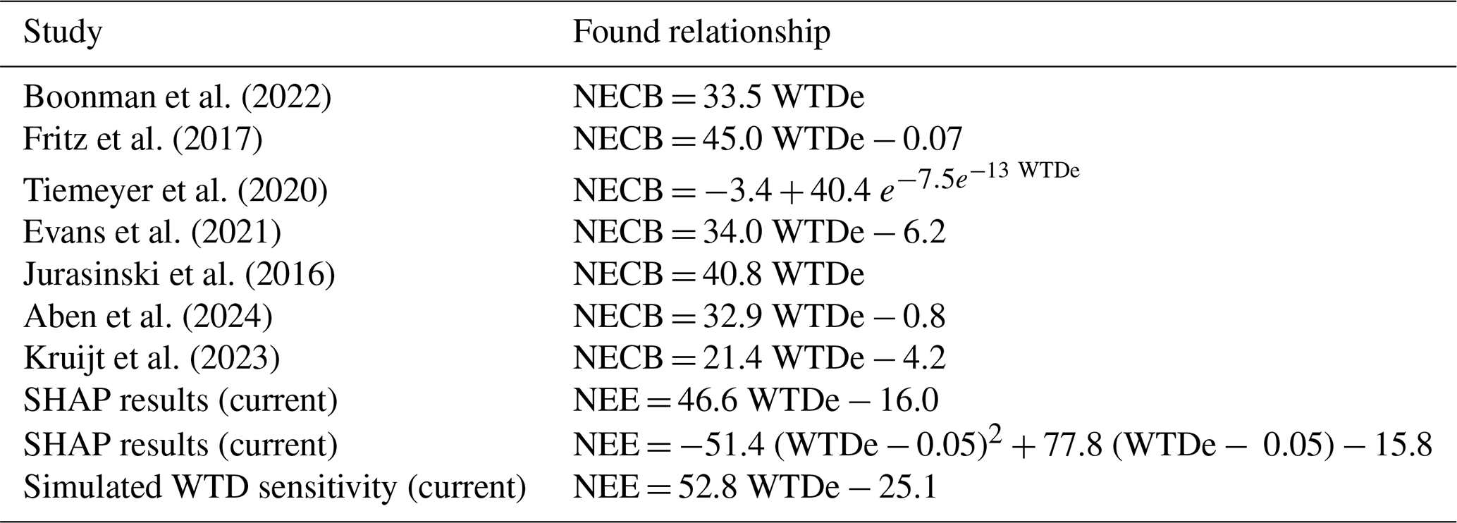
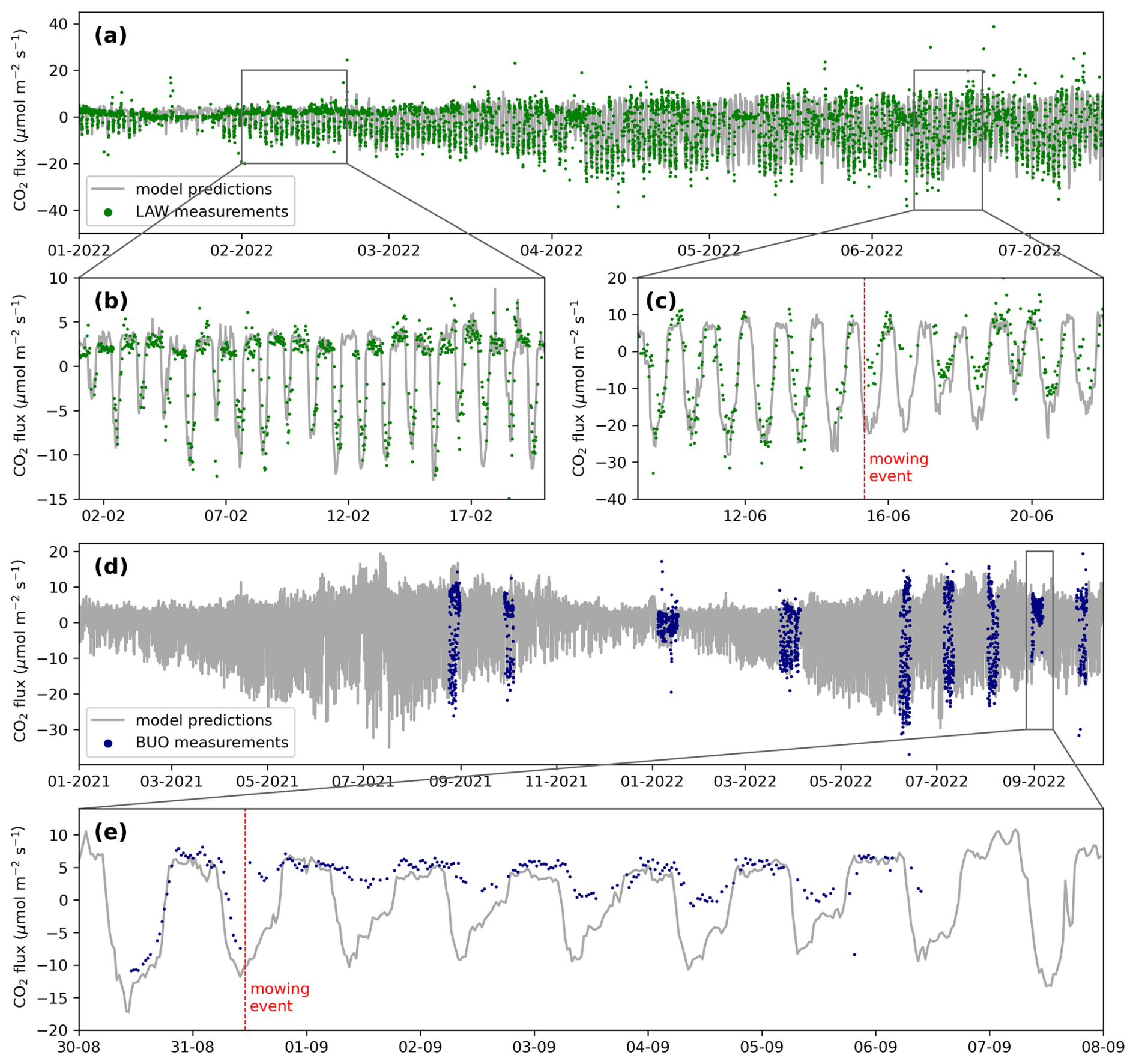
Figure H1 Predictions and measurements of CO₂ flux at LAW (a–c) and BUO (d, e). In (c) and (e), mowing events are highlighted with a red line. In (e), uptake immediately stops after mowing, whereas in (c), there is still uptake after mowing, which decreases the day after. We hypothesize this is due to the mowing of different parcels at LAW on different days, possibly by the neighboring farmer.

Appendix I: Shannon entropy

Table I1 Results of Shannon entropy in our datasets for all regions combined.

$$\begin{array}{}\text{(I1)}& A_H=\mathrm{1}-{\displaystyle \frac{H\left({\mathrm{CO}}_{\mathrm{2}\mathrm{mod}}\right)}{H\left({\mathrm{CO}}_{\mathrm{2}\mathrm{obs}}\right)}},\end{array}$$

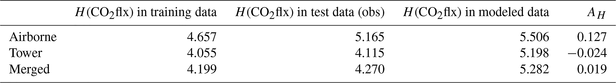
where H is Shannon entropy, and CO₂ mod and obs are modeled and observed CO₂ fluxes. The best model perfectly reflects the entropy in the observed data such that A_H = 0.