the Creative Commons Attribution 4.0 License.
the Creative Commons Attribution 4.0 License.
 | 26 Aug 2025
Inferring methane emissions from African livestock by fusing drone, tower, and satellite data
Alouette van Hove
Kristoffer Aalstad
Vibeke Lind
Claudia Arndt
Vincent Odongo
Rodolfo Ceriani
Francesco Fava
John Hulth
Norbert Pirk
Considerable uncertainties and unknowns remain in the regional mapping of methane sources, especially in the extensive agricultural areas of Africa. To address this issue, we developed an observing system that estimates methane emission rates by assimilating drone and flux tower observations into an atmospheric dispersion model. We used our novel Bayesian inference approach to estimate emissions from various ruminant livestock species in Kenya, including diverse herds of cattle, goats, and sheep, as well as camels, for which methane emission estimates are particularly sparse. Our Bayesian estimates aligned with Tier 2 emission values of the Intergovernmental Panel on Climate Change. In addition, we observed the hypothesized increase in methane emissions after feeding. Our findings suggest that the Bayesian inference method is more robust under non-stationary wind conditions compared to a conventional mass balance approach using drone observations. Furthermore, the Bayesian inference method performed better in quantifying emissions from weaker sources, estimating methane emission rates as low as 100 g h−1. We found a ± 50 % uncertainty in emission rate estimates for these weaker sources, such as sheep and goat herds, which reduced to ± 12 % for stronger sources, like cattle herds emitting 1000–1500 g h−1. Finally, we showed that radiance anomalies identified in hyperspectral satellite data can inform the planning of flight paths for targeted drone missions in areas where source locations are unknown, as these anomalies may serve as indicators of potential methane sources. These promising results demonstrate the efficacy of the Bayesian inference method for source term estimation. Future applications of drone-based Bayesian inference could extend to estimating methane emissions in Africa and other regions from various sources with complex spatiotemporal emission patterns, such as wetlands, landfills, and wastewater disposal sites. The Bayesian observing system could thereby contribute to the improvement of emission inventories and verification of other emission estimation methods.
- Article
(5329 KB) - Full-text XML
-
Supplement
(23681 KB) - BibTeX
- EndNote


Global mean atmospheric methane (CH4) mixing ratios reached 1.93 ppm in 2024, marking a 16 % increase since 1985 (Lan et al., 2024). Livestock production is a major contributor to global anthropogenic CH4 emissions, accounting for approximately one-third of the total emissions (Saunois et al., 2020). Within this sector, enteric fermentation in ruminants – such as cattle, sheep, goats, and camels – is the predominant source, generating approximately 80 % of these emissions, while the remainder originates from manure (Amon et al., 2001). During the digestive process, CH4 is produced by rumen fermentation, with about 90 %–95 % released through burping and 5 %–10 % as intestinal gas (Broucek, 2014). Due to its high global warming potential and relatively short atmospheric lifetime, reducing CH4 emissions can have quick benefits in mitigating climate change (Szopa et al., 2021). Therefore, accurate measurements and understanding of CH4 emissions from ruminants are important for developing effective mitigation strategies and evaluating their efficacy.
The Intergovernmental Panel on Climate Change (IPCC) provides standardized methodologies for estimating CH4 emissions from ruminants (Gavrilova et al., 2019). Tier 1 methods use generalized default values for emission factors that are often region-specific, while Tier 2 values incorporate more detailed herd-specific data, accounting for local variations in livestock management and environmental conditions. Recent studies from sub-Saharan Africa demonstrate substantial differences between estimates from these two tiers (Goopy et al., 2018; Ndung'u et al., 2019; Gurmu et al., 2024), highlighting the need for precise and locally relevant data. However, there is a scarcity of studies focusing on CH4 emission rates from ruminants in this region, with many relying on metabolic energy balance estimates based on factors such as animal weight, feed, and activity level, and only a few studies using direct CH4 measurements (e.g., Korir et al., 2022a; Goopy et al., 2020; Mwangi et al., 2023; Wolz et al., 2022). Specifically, research on CH4 emissions from camels is sparse. Although a few studies have estimated emissions using direct CH4 measurements from smaller camelids such as alpacas and llamas (e.g., Pinares-Patiño et al., 2003; Nielsen et al., 2014), research on larger camelids, like dromedaries and Bactrian camels, remains limited. This lack of data is likely due to size limitations of respiration chambers for measuring gas exchange. Nonetheless, Dittmann et al. (2014) conducted respiration chamber measurements with Bactrian camels.
Gas exchange methods such as respiration chambers and headboxes are typically used to quantify CH4 emissions from individual animals. For estimating emissions from ruminant herds or entire farm facilities, several indirect techniques have been applied. Tracer-ratio experiments (Vechi et al., 2022; Daube et al., 2019; Arndt et al., 2018) involve releasing a tracer gas and comparing its dispersion to that of CH4. The mass balance approach (Vinković et al., 2022; Arndt et al., 2018; Wratt et al., 2001) calculates emissions based on the difference between incoming and outgoing CH4 flux estimates within a defined volume. Some studies (Wolz et al., 2022; Bai et al., 2021; Arndt et al., 2018) use open-path Fourier transform infrared or laser spectrometry to obtain horizontal path-integrated CH4 concentrations upwind and downwind from the source, which are combined with a Lagrangian particle dispersion model to estimate emission rates. Inverse modeling techniques (Andersen et al., 2021) infer emission rates by fitting an atmospheric dispersion model to measured atmospheric data. On larger spatial scales, typically spanning multiple kilometers, satellite observations are used to detect and quantify CH4 emissions from super-emitters, such as oil and gas leaks and landfills (e.g., Pandey et al., 2019; Dogniaux et al., 2024). However, the smaller emission rates of livestock herds are more challenging to detect using satellite data, necessitating measurement platforms with a higher spatial resolution. Drone technology provides a solution, enabling high-resolution spatiotemporal observations of atmospheric gases and thermodynamic variables (Villa et al., 2016; Burgués and Marco, 2020). Our study uses drones to sample CH4 emission plumes from nine different ruminant herds in Kenya, leveraging these data for emission estimation.
Our study employs an innovative Bayesian inference approach, using a sequential Monte Carlo method to invert an atmospheric dispersion model. This method combines observed data with prior information to enhance emission estimation. A key advantage of Bayesian inference is its ability to integrate noisy observations from multiple platforms, including drones and flux towers. The framework's probabilistic approach systematically accounts for observation uncertainties, potentially improving the precision and reliability of our emission estimates. We assess the efficacy and robustness of this novel method by comparing our results with those obtained from a conventional mass balance method and IPCC emission values. To complement this analysis, we assess the capability of hyperspectral satellite data to pinpoint the location of CH4 sources, specifically ruminant herds, by identifying spectral anomalies at the landscape level. Our objectives are as follows: (1) to evaluate the efficacy of the Bayesian inference method utilizing drone-based observations for estimating CH4 emission rates; (2) to determine emission rates for free-grazing cattle, sheep, goats, and camels in a sub-Saharan African country using drone-based observations; (3) to compare the results obtained from the novel Bayesian inference method with estimates from a more traditional mass balance method and IPCC emission values, evaluating different methods for estimating CH4 emissions from ruminants and contributing to improving national greenhouse gas inventories; and (4) to investigate whether spectral indices related to CH4 emissions from hyperspectral satellite data can assist in detecting locations of CH4 sources, specifically ruminant herds.
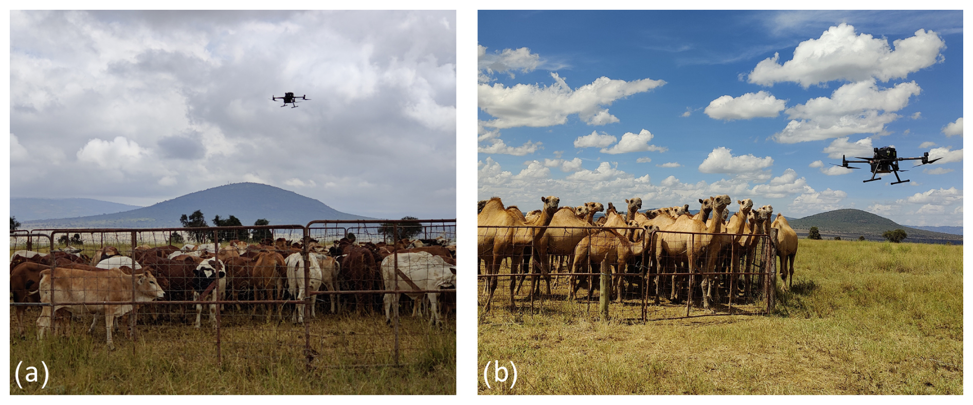
Figure 1(a) A drone flight capturing methane concentration observations of a heifer herd coinciding with the satellite overpass on 6 March 2024. (b) Camels inside a boma during a drone flight on 4 March 2024. Of all the animals, the camels were the most curious about the drone.
This study was conducted at the Kapiti Research Station in Kenya, approximately 60 km southeast of Nairobi. The station is managed by the International Livestock Research Institute (ILRI). Covering over 13 000 ha, the station houses various ruminants, including cattle, sheep, goats, and camels, with a primary focus on studying livestock productivity and a secondary focus on the conservation of migratory wildlife species. Kapiti is located in Kenya's semi-arid savanna, characterized by a diversity of savanna grasses, shrubs, and scattered Acacia trees. Livestock management at Kapiti follows typical pastoral systems, where herders allow the animals to graze freely during the day and keep them in enclosures, known in Kenya as bomas, during the night. Apart from livestock, there were no other known CH4 sources of considerable magnitude close to the study site. The net savanna soil background flux was estimated to be nearly zero. Measurements recorded by the eddy-covariance tower at the study site indicated values of 0.4 ± 2.6 during the drone flights and 0.7 ± 3.7 throughout the period of the measurement campaign. This finding is further supported by chamber measurements conducted at the study site over the entire year of 2017, which reported a net flux of 0.1 ± 0.7 (Leitner et al., 2024). Consequently, we considered the savanna soil background flux to be negligible.
This section outlines four methods that were used to detect and estimate CH4 sources: (1) source term estimation through drone observations using an innovative particle-based Bayesian inference method, (2) source term estimation through drone observations using a traditional mass balance approach, (3) calculation of IPCC Tier 2 emission values, and (4) detection of potential CH4 source locations through hyperspectral satellite observations at the landscape level. Although the latter is not a direct source term estimation method, we evaluated whether radiance anomalies in satellite data could effectively detect potential CH4 sources to guide targeted drone missions for further investigation and quantification.
2.1 Drone-based source term estimation
This section provides details of the drone field campaign, conducted between 29 February and 7 March 2024 at Kapiti. It outlines both the Bayesian inference method and the mass balance approach used to estimate CH4 emission rates from drone observations.
We used a drone equipped with a gas sensor to obtain CH4 concentration observations of the emission plumes of nine different ruminant herds: cattle (cows, heifers, steers, and slick herd), sheep (lactating ewes), goats (dry does, pregnant does, and weaner kids), and camels. The cows, heifers, and steers were Boran cattle, while the slick herd consisted of a crossbreed between Holstein–Friesian and Boran heifers. The sheep flock included Red Masaai and Dorper, and the goat herds comprised Small East African and Galla varieties. The camels were dromedaries. The lactating ewes had lambs, and the pregnant does had kids with them. However, because the rumen fermentation systems of milk-fed lambs and kids are not yet fully developed (Baldwin et al., 2004), we assumed their CH4 emissions to be negligible and treated these herds as if the lambs and kids were not present. The herd sizes are included in Table B1. During the drone flights, the respective herds were confined within a boma at coordinates −1.6136° N, 37.13234° E. The animals exhibited no signs of distress and appeared at ease throughout the drone operations. Figure 1 shows the heifers inside the boma, as well as a herd of camels observing a passing drone.
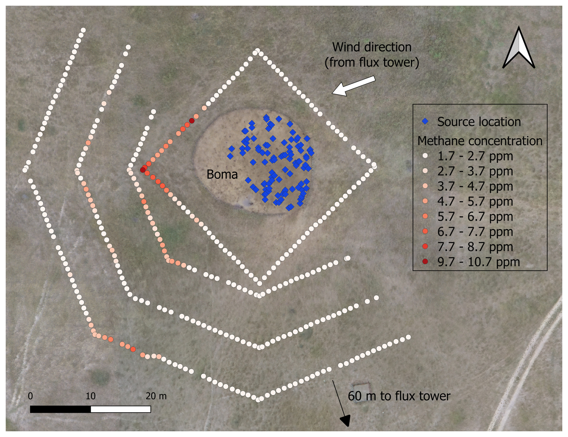
Figure 2Top-down view of the drone flight paths capturing methane observations in the afternoon of 6 March 2024. Shown are methane mixing ratio measurements obtained at a height of 2.7 m during the mass balance flight around the boma and at heights of 3.5, 3.0, and 2.5 m during the half-octagon flight for the Bayesian inference method. The blue markers indicate the source location in the atmospheric dispersion model, representing the heifer herd. The wind direction arrow shows the mean wind direction observed at the flux tower.
Typically, four flights were conducted for each ruminant herd. In the morning, before grazing, two flights were performed: one flight for each emission estimation method. The Bayesian inference flight focused on monitoring the downwind emission plume at various distances and altitudes from the source. In contrast, the mass balance flight, following Gålfalk et al. (2021), involved flying a virtual box around the source, capturing the differences in CH4 concentrations upwind and downwind from the source. The same set of flights was repeated in the afternoon after the animals had grazed. Feed intake is known to increase enteric CH4 emissions in ruminants, with peak emissions occurring shortly after feeding (Amon et al., 2001; Hegarty, 2013). Because the animals had no access to feed during the night, lower emissions are expected in the morning compared to the afternoon, following grazing. We investigated whether there was a noticeable increase in CH4 emissions between the morning and afternoon flights, using consistent observations of such increases as indicators of the method's reliability and accuracy. During control drone flights, conducted without animals present in the boma or the immediate surroundings, no increase in CH4 levels was observed throughout the field campaign. Consequently, we assumed that CH4 production from manure was negligible, attributing the elevated CH4 concentration observations solely to enteric fermentation. This is supported by Leitner et al. (2024), which found that boma manure contributes only 2.2 % to total CH4 emissions at Kapiti.
2.1.1 Observing system
Our observing system consisted of a drone (DJI Matrice 300 RTK, DJI, China) equipped with a CH4 gas sensor (MIRA Strato LDS, Aeries Technologies, USA), as well as a stationary flux tower with an eddy-covariance system (Burba, 2013). The tower was located at coordinates −1.61419° N, 37.13313° E, approximately 100 m south-southeast from the center of the boma, as shown in Fig. 2. The drone's position was recorded using real-time kinematic (RTK) positioning. A digital elevation model (DEM) of the area was obtained using lidar (Zenmuse L1, DJI, China), processed in DJI Terra. The altitude data from the RTK system were corrected using the DEM at the drone's home location. Additionally, the DEM was used to determine the drone's flight height above the ground surface.
The gas analyzer detects CH4 using mid-infrared laser spectroscopy, which measures the absorption of infrared radiation by CH4 molecules. The reported mixing ratio X [ppm; parts per million per volume] at the point of measurement is the fraction of CH4 molecules per million molecules of air. The sensor has a sensitivity of 0.001 ppm and a sampling rate of 1 Hz. The sensor was factory calibrated and has an expected drift of 0.01 to 0.05 ppm since calibration (from communication with the manufacturer). The mixing ratio X was converted to mass concentration c [g m−3] using the ideal gas law, with the ambient air temperature and pressure obtained from the flux tower.
Wind data were collected using two sensor platforms: a fixed flux tower and the drone. Wind data were captured by a 3D sonic anemometer (WindMaster, Gill Instruments, UK) mounted on the tower at a height of 5 m above the ground. The wind speed and wind direction data were resampled from 10 to 1 Hz to match the timestamps of the CH4 sensor. The data from the eddy-covariance system were processed at half-hour intervals using EddyPro software (Li-Cor, USA) to determine the Obukhov length L [m] and friction velocity u∗ [m s−1]. Using Monin–Obukhov similarity theory (MOST; see Stull, 1989), we estimated the vertical profile of the mean wind speed V(z) [m s−1] and mean eddy diffusivity K(z) [m2 s−1], where z is the distance above the ground. Appendix A includes details on the application of MOST.
The drone quantifies wind speed using its onboard sensors to measure resistance during stable hover or flight. These data, combined with the drone's GPS and inertial measurement unit (IMU), allow for estimations of wind speed and direction by analyzing the accelerations and attitude adjustments needed to counteract the wind's force (Abichandani et al., 2020). Wind data from the drone were obtained from the flight logs using the Flight Reader software.
Given concerns that the additional bulk and weight of the CH4 sensor might affect readings, we performed a correction for wind speed. During the field campaign, the drone hovered for a total of 90 min a couple of meters downwind from the sonic anemometer under various wind speeds and orientations relative to the wind direction. Wind speed data from the drone were corrected through linear regression against the sonic anemometer data (Fig. S1 in the Supplement). The wind direction is reported by the drone in eight compass directions. The wind direction data did not qualitatively match well with the sonic anemometer data and were therefore not used in our study (Fig. S2).
2.1.2 Bayesian inference method
The first drone-based method for quantifying CH4 emission rates utilizes an inverse modeling approach. Model inversion involves estimating unknown input parameters of a theoretical model by utilizing observed data related to the output variables. We assimilated atmospheric measurements into an atmospheric transport model to infer emission rates. Two principal approaches are commonly employed in model inversion: (1) several studies (Andersen et al., 2021; Shah et al., 2019, 2020) minimize a cost function to find the best fit between a Gaussian plume model (Sutton, 1947) and observed CH4 concentrations using a frequentist framework. (2) In the field of robotics, various studies employ Bayesian inference for model inversion to estimate source emission rates and source locations, among other unknown variables, at local scales (Hutchinson et al., 2017; Francis et al., 2022). The Bayesian approach is particularly well suited to solving ill-posed inverse problems involving the assimilation of noisy observations that are ubiquitous in geophysics (Sanz-Alonso, 2023). Beyond robotics, Bayesian frameworks are also utilized in estimating carbon emissions on regional or global scales from satellite observations (Cusworth et al., 2021; Western et al., 2021) and international ground-based atmospheric observation networks (Evangeliou et al., 2018; Thompson et al., 2022).
We adopted a Bayesian approach, providing a probabilistic interpretation of the model parameters, including uncertainty quantification. Previous research has demonstrated the efficacy of Bayesian inference with synthetic drone observations for source localization and estimation (Loisy and Eloy, 2022; van Hove et al., 2023, 2024b). However, its applications in real-world environments at a local scale remain relatively limited. Hutchinson et al. (2019) and Park et al. (2021) successfully deployed Bayesian inference methods in outdoor experiments with flat, homogeneous terrain and time-invariant controlled-release sources, while Hutchinson et al. (2020) explored emissions from a car crash and oil rig at a test site. In real-world conditions, Pirk et al. (2022) assimilated drone observations within a Bayesian framework to infer turbulent fluxes of sensible and latent heat of a wetland and a palsa mire in Norway.
We used the advection–diffusion model formulated by Vergassola et al. (2007) to simulate CH4 transport under turbulent atmospheric conditions. This model has been shown by Hutchinson et al. (2019) to more accurately represent small-scale plume behavior compared to the Gaussian plume model. With a single point source, the mean stationary concentration c [g m−3] at measurement location is given by
where represents the source location, Qs [g h−1] denotes the CH4 point source emission rate, α = 3600 s h−1 is the time conversion factor from hours to seconds, V [m s−1] represents the mean wind speed, ϕ [°] is the mean wind direction, D [m2 s−1] denotes the effective diffusivity, λ [m] is a characteristic length scale, and c0 [g m−3] is the mean stationary background concentration. We make a distinction between the total emission rate of the entire herd, denoted by Q [g h−1], and the emission rate per individual animal, denoted by q [g per head per hour].
Each of the meteorological parameters in Eq. (1) influences different aspects of the emission plume. Specifically, the wind direction determines the plume's orientation, while wind speed and diffusivity influence the plume's shape, and the emission rate determines how elevated the plume's concentration level is above the background. The instantaneous wind fluctuates in amplitude and direction due to turbulent forces, which are influenced by the effective diffusivity D. The effective diffusivity is the sum of the turbulent diffusivity and the typically much smaller molecular diffusivity. Unlike the Gaussian plume model, which uses dispersion parameters σy and σz, typically determined by the stability classification schemes of Pasquill (1961), effective diffusivity D is directly incorporated in the model. Consequently, by making the assumption D≈K, observational estimates of D can be obtained via MOST, as detailed in Appendix A.
The length scale λ in Eq. (1) is defined as
where D denotes the effective diffusivity, V is the mean wind speed, and τ is the finite lifetime of CH4 in the atmosphere, approximately 9.1 years (Prather et al., 2012).
To conserve CH4 mass in Eq. (1), the ground was modeled as a perfect reflector of the plume, as is typically done in Gaussian plume modeling (Hanna et al., 1982). This was achieved by including a mirror image source below the ground surface: . Consequently, the total concentration field is expressed as the sum of the original and mirrored sources: .
In our study, emission rate Qs, mean wind speed V, mean wind direction ϕ, and effective diffusivity D in Eq. (1) are treated as unknown parameters to be inferred through model inversion. The parameters that are assumed to be known include the source location xs, drone locations x, and background concentration c0, which have been determined as follows. On the small spatial scale of our study, approximating the herd of animals as a single point source would be an oversimplification. Instead, we modeled the herd as a set of m point sources, resulting in a total concentration field that is the sum of the individual concentration anomalies from these sources: . This source superposition is commonly used in Gaussian plume modeling (e.g., Calder, 1977). Using aerial photographs taken during the drone flights, we randomly selected m=100 source locations within the outline of the herd, which together are responsible for a total emission rate Q=mQs. For example, the 100 blue markers within the boma shown in Fig. 2 represent the source location of a heifer herd. After inferring the total emission rate Q, we normalized it by the actual number of animals na in the herd to obtain the emission rate per individual animal . The source height zs was estimated by averaging the mouth height of 10 animals from each herd, based on direct measurements. The majority of the CH4 mixing ratio measurements for each drone flight were below 1.8 ppm. The mean background concentration c0 was determined as the median of the converted CH4 observations that fell below this threshold. Although this value is lower than the global average mixing ratio of 1.93 ppm, measurements in Norway before and after the field campaign were close to the global average, and data inspection by the manufacturer revealed no sensor abnormalities, suggesting that this low value was natural. Addressing any remaining concerns, we note that both drone methods rely on concentration elevations above the background level, ensuring that any potential systematic bias does not affect the final estimates.
The drone flew nine legs in a half-octagon pattern downwind of the herd at three different distances: approximately 40, 30, and 20 m from the center of the boma. The corresponding heights for the outer legs were approximately 3.5, 5.5, and 9.0 m; for the middle legs, 3.0, 4.5, and 7.0 m; and for the inner legs, 2.5, 3.5, and 5.0 m above ground level. To minimize the effects of rotor downwash (visualized with colored smoke in Crazzolara et al., 2019) and downwind disturbances to the plume (visualized with colored smoke in Hutchinson et al., 2019), the flights were performed from the outer to the inner legs, starting at the lowermost altitude and ascending to higher altitudes. Figure 2 offers a top-down view of the boma and illustrates the measured CH4 mixing ratios along the lowest three legs of the half-octagon flight plan during the drone flight with a herd of heifers.
We explore the use of three different observing systems for model inversion, i.e.,
- a.
CH4 concentration data: we assimilated only instantaneous drone-based CH4 mixing ratio data X, which were converted to CH4 concentration c, for use as observations.
- b.
CH4 concentration data with drone-derived wind speed: we assimilated the same concentration data (observation case (a)) along with mean wind speed observations Vobs derived from drone data. The average wind speed was calculated over the estimated plume depth of 8 m. Specifically, wind speed data from the drone flight were averaged over 1 m vertical intervals up to 8 m, and the overall average was obtained over these interval-specific averages.
- c.
CH4 concentration data with flux tower data: we assimilated CH4 concentration data (observation case (a)) in combination with observations for mean wind speed Vobs, mean wind direction ϕobs, and effective diffusivity Dobs derived from the flux tower data. In this case, we approximated that D≈K and assumed that the vertical and horizontal diffusivity are equal, as is done in Eq. (1). We obtained mean wind speed and diffusivity values by averaging their respective profiles – Eqs. (A1) and (A3) – over the estimated vertical plume extent of 8 m.
We employ a probabilistic approach to model inversion, applying Bayesian inference recursively to mini-batches of observational data to make the problem more computationally tractable (Chopin, 2002). At each new iteration step n+1, the dynamic prior probability distributions of the unknown parameters are updated to the posterior probability distributions given a new mini-batch of observations dn+1 via Bayes' rule:
where the conditional model evidence (or marginal likelihood) acts as a normalizing constant:
At each new iteration n+1, the dynamic prior distributions are simply the corresponding dynamic posteriors from the previous iteration n. The use of such sequential Bayesian updating makes the inference problem more computationally tractable and is a key property of the sequential Monte Carlo methods that we employ in practice (Chopin and Papaspiliopoulos, 2020). Note the slight abuse of notation where d0 is implicitly empty, and thus p(θ|d0) – rather than the usual p(θ) – denotes the initial prior at n=0 for notational convenience.
The likelihood term in Eq. (3) links the observations to the forward model, effectively serving as a measure of discrepancy between the observed data and the model predictions. The observational model relating observations d to the forward model prediction is given by
where ϵ represents the discrepancy (or residual) term, explicitly capturing the various sources of error in the measured data (and implicitly also errors in the model). For the CH4 concentration observations cobs, the forward model ℱ is based on Eq. (1) for m sources. In the case of the wind and diffusivity observations, ℱ is a more direct noisy mapping; for example, the observed mean wind speed Vobs is modeled as .
As Rao (2005) identifies, discrepancies in atmospheric dispersion modeling can arise due to: (a) noise in the sensor measurements, (b) errors in the model input data, (c) the fact that atmospheric dispersion models are imperfect, and (d) inherent randomness in unresolved turbulent dispersion processes. Given the limited knowledge of these errors, the Gaussian distribution is the most conservative choice for the likelihood function according to the maximum entropy principle (Jaynes, 2003). Thus, we define the likelihood function as a Gaussian of the form , where the mean vector ℱ(θ) contains the model predictions and R is a diagonal observation error covariance matrix with observation error variances σ2 along the diagonal. These observation error variances correspond to the respective observation error standard deviations empirically estimated as σc = 0.54 mg m−3 (corresponding to 1 ppm), σV = 0.30 m s−1, σϕ = 10°, and σD = 0.15 m2 s−1 for concentration c, mean wind speed V, wind direction ϕ, and effective diffusivity D, respectively.
We recognize a discrepancy between the timescales of our concentration observations and the statistical assumptions of our dispersion model presented by Eq. (1): while the observations are instantaneous samples of a turbulent boundary layer, our model represents a time-averaged plume. This discrepancy or representation error (van Leeuwen, 2015) is expected to be the largest source of uncertainty in our Bayesian inference approach. Additional sources of uncertainty include the assumption of a fixed vertical plume extent, ignoring uncertainties inherent in the (assumed) known variables such as the background concentration, among other factors. To account for these approximations and minimize the impact of potential errors, we incorporate a high level of uncertainty into the likelihood term by inflating the observation error covariance R to match the aforementioned observation error standard deviations.
The initial prior distributions p(θ|d0) are chosen to be flat non-informative priors in the form of uniform distributions across defined ranges to match reasonable prior expectations (Banner et al., 2020): g per head per hour, m s−1, °, corresponding to the wind compass half of the prevailing wind direction, and m2 s−1. We implement the Bayesian inference framework in Python (available from van Hove et al., 2024a) by a sequential Monte Carlo (SMC) framework (Chopin and Papaspiliopoulos, 2020; Särkkä and Svensson, 2023) that generalizes the classic bootstrap particle filter (Gordon et al., 1993). This method approximates the probability distributions with a set of weighted ensemble members, referred to as particles. In each iteration, the weights of these particles are updated based explicitly on their likelihood, representing their fit to the observed data, and implicitly on the dynamic prior. To address the particle degeneracy problem, where only a few particles retain significant weights, we apply the resample-move algorithm (Gilks and Berzuini, 2001; Doucet and Johansen, 2009). This algorithm enhances the particle diversity and exploration of the parameter space by combining resampling with subsequent Markov chain Monte Carlo (MCMC) moves. Additionally, reflective boundaries are used to respect the predefined ranges of the prior uniform distributions. In our algorithm, we use 25 000 particles and a mini-batch size of 200 observations, and we perform five MCMC steps per iteration step.
Due to the inherently stochastic nature of the SMC algorithm, different realizations can yield varying results. This variability arises from randomness in the prior sampling, the generation of proposals in each MCMC step, the selection of the mini-batches of observations, and the determination of the m source locations representing the herd. As a result, it is common practice to run the SMC algorithm multiple times to (a) assess the variability of its output and (b) obtain more reliable statistical estimates of the inferred parameters (Chopin and Papaspiliopoulos, 2020; Vergé et al., 2015). Thereby, we perform 22 independent realizations of the SMC algorithm in an outer loop to derive more robust estimates of the CH4 emission rates.
The methodological challenges encountered during the implementation of the Bayesian inference method are discussed in Sect. 3.4.
2.1.3 Mass balance method
The second drone-based method for quantifying CH4 emission rates uses a mass balance approach. Based on the divergence theorem, this technique determines the emission rate from a CH4 source by assessing the net horizontal inflow and outflow of CH4 within an imaginary box enclosing the source. The mass balance approach, or box model, has been widely utilized with drone observations in various studies. For example, Allen et al. (2019) and Gålfalk et al. (2021) estimated emissions from landfills, while Andersen et al. (2021) determined emissions from coal mining ventilation shafts, and Vinković et al. (2022) investigated emissions from a dairy farm. Additionally, Golston et al. (2018) and Yang et al. (2018) applied the mass balance method with a laser-based CH4 sensor capturing a column-integrated concentration along a vertical path between the drone and the ground to investigate natural gas leaks. On larger scales, the method has been applied using aircraft observations. For example, Cambaliza et al. (2014) assessed emissions of an urban region including multiple sources such as power plants, landfills, and wastewater treatments, while Arndt et al. (2018) quantified emissions of dairy farms encompassing animal housing and liquid manure storage. On regional or global scales, mass balance analysis is used to estimate emission rates from satellite observations (e.g., Pandey et al., 2019; Borchardt et al., 2021). However, Varon et al. (2018) notes that this method is susceptible to large errors. This is due to the inability to accurately parameterize turbulence on the small scale of instantaneous plumes, as well as poor characterization of the vertical wind speed profile between the ground surface and satellite.
The drone collects CH4 point measurements along the vertical planes of an imaginary box encapsulating the source. Data are then interpolated onto a regular grid to calculate the net emission rate Q [g h−1] by integrating the product of CH4 concentration c [g m−3] and outward perpendicular wind speed across the vertical sampling planes:
where v⟂ [m s−1] denotes the instantaneous wind speed outward perpendicular to the plane, a [m2] is the area of a grid cell, α = 3600 s h−1 is the time conversion factor from hours to seconds, ki is the number of horizontal grid cells of a plane, and kj is the number of vertical grid cells of a plane.
The vertical sampling planes must be sufficiently high to capture the full extent of the emissions so that there are only negligible fluxes through the top horizontal plane of the imaginary box. Our imaginary box around the boma measures approximately 26 m by 26 m with a height of 10 m. To mitigate downwash effects from the rotors, the drone's flight plan was designed from the ground up. The drone first performed a manual flight at around 1.0 m above the ground for the lowest leg, followed by a pre-planned flight mission with ascending legs at approximately 2.0, 2.7, 3.7, 5.2, 7.2, and 9.2 m. The drone flew at 1 m s−1, collecting observations approximately every meter. Figure 2 displays the measured CH4 mixing ratios at a height of 2.7 m during a flight with the heifer herd.
To evaluate Eq. (6), we used the horizontal instantaneous corrected wind speed data from the drone and wind direction observations from the sonic anemometer on the flux tower, which we considered more reliable than the drone's wind direction estimates. Artificial wind speed data points of 0 m s−1 were added at ground level to account for the no-slip lower boundary condition. The CH4 concentration and perpendicular wind speeds were interpolated onto northeast (NE)-, southeast (SE)-, southwest (SW)-, and northwest (NW)-facing vertical planes. Following the general approach of Gålfalk et al. (2021), we resampled the observations using the following sequence of steps: (a) linear interpolation of the data points onto a regular grid of circa 20 cm2, (b) averaging onto a coarser grid of circa 1 m2, and (c) filling any remaining empty grid cells, if any, using nearest-neighbor values.
The current sampling time of approximately 20 min is insufficient to capture the mean state of the plume morphology, introducing uncertainty into the emission rate estimate. This primarily stems from temporal variability induced by unresolved atmospheric turbulence affecting wind speed and wind direction (σv,temp and σϕ,temp). This is further complicated by potential wake effects from the herd that disturb the mean flow field, influencing wind speed observations in the downwind sampling plane. Additionally, measurement uncertainties in wind speed and wind direction (σv,meas and σϕ,meas) further contribute to the overall uncertainty in the mass balance approach. Moreover, the wind direction's assessment at the flux tower, rather than at the vertical planes, introduces additional uncertainty. The measurement uncertainty of the CH4 observations is minimal and considered negligible compared to wind-related uncertainties. Similarly, the relative uncertainty of the interpolation process is considered minor and is excluded from the overall uncertainty estimate. Our approach to uncertainty estimation for the mass balance method aligns with the practices outlined in Andersen et al. (2021).
We estimated uncertainties due to temporal variation in wind speed and direction (σv,temp and σϕ,temp) based on their standard deviation from the mean at the altitude of each leg of the drone flight, following the methodology presented in Cambaliza et al. (2014). Measurement uncertainties for wind speed and wind direction were estimated at σv,meas = 1.7 m s−1 and σϕ,meas = 20°, respectively. The wind speed uncertainty estimate was derived from the root mean square error between the corrected wind speed readings from the drone and wind speed records from the sonic anemometer during hovering flights; see Sect. 2.1. The temporal variation and measurement uncertainty were summed in quadrature: and . Finally, the total uncertainty estimate for the emission rate was determined through error propagation (Gålfalk et al., 2021; Andersen et al., 2021; Vinković et al., 2022). A Monte Carlo approach with 500 runs was used for error propagation (Anderson, 1976) to incorporate the various uncertainty sources.
2.2 IPCC Tier 2 emission values
In addition to drone-based methods, we estimated CH4 emissions from enteric fermentation of ruminant herds using the IPCC Tier 1 and Tier 2 approaches (Paustian et al., 2006). The Tier 1 method uses generalized default values for the emission factor EF [kg per head per day], often specific to regions or continents. In contrast, the Tier 2 method incorporates more detailed, herd-specific or animal-specific data, making Tier 2 values generally more reliable than Tier 1 estimates. This method is based on the typical daily metabolic energy balance of the animals, where the CH4 emission factor EF is calculated by
where Ym denotes the fractional methane conversion factor, G [MJ per head per day] is the gross energy intake, and E = 55.65 MJ kg−1 is the energy content of CH4. The daily gross energy intake per animal G is determined from information on feed quality and feed intake, live weight of the animals, weight changes, and productivity parameters (as specified in Eq. 10.16 in Paustian et al., 2006). These data can be obtained at the herd level, the individual animal level, or a combination of both. Methane conversion factor Ym represents the fraction of gross energy intake converted to CH4. The IPCC provides Ym values for different animal categories based on a review and synthesis of available scientific literature and data (cattle values in Table 10.12 and sheep and goat values in Table 10.13 of Paustian et al., 2006). Because specific values are currently unavailable for camels and we do not have the live weight of the camel herd from our drone flights, we use the IPCC Tier 1 value for camels in our study.
At Kapiti, all livestock herds graze freely during the day, and we assume that their feed intake is entirely from pasture. The feed quality of the pasture was determined by averaging the nutrient content of 19 samples collected from different locations across Kapiti on 1 March 2024. These samples were analyzed for dry matter content, nitrogen (converted to crude protein), carbon, ash, and fiber-fractions (NDF: neutral detergent fiber; ADF: acid detergent fiber; ADL: acid detergent lignin). These data were used to compute feed digestibility, representing the portion of gross energy intake in the feed not excreted in feces. Data on average feed intake are difficult to obtain from grazing animals and were therefore estimated.
The live weight [kg] and time-average daily live weight change [kg d−1] of individual animals were determined from direct measurements taken during the first half of March 2024 and then again at the end of April or May 2024. The average weight and daily weight change across all animals in a herd were used to compute the EF for the respective animal category. Additional data used to estimate gross energy intake for each animal herd include the following: proportion of pregnant females (84 % of pregnant does herd, 30 % of cow herd, and 30 % of slick herd); proportion of lactating females (87 % of lactating ewes flock) with average milk production (1.5 ); number of offspring; and an estimate for the animal's activity, specifically the daily walking distance on the pasture [km d−1]. We convert the resulting emission factor EF [kg per head per day] into emission rate q [g per head per hour] for each animal category to enable method comparison in our study. With the exception of weight and weight changes, all parameters were estimated at the herd level without accounting for associated uncertainties. As we did not perform an explicit uncertainty assessment for the IPCC values, we apply a ± 20 % uncertainty range for Tier 2 values and a ± 30 % to ± 50 % uncertainty range for the Tier 1 values, as reported by the IPCC (Paustian et al., 2006).
2.3 Satellite observations for source detection
In an exploratory effort, we investigated the potential for detecting livestock herds as CH4 sources using satellite hyperspectral imagery. On 6 March 2024, the PRecursore IperSpettrale della Missione Applicativa (PRISMA) satellite (Loizzo et al., 2018) was commissioned to capture a hyperspectral image of Kapiti specifically for this research while three cattle herds were present at different locations. The PRISMA satellite has two hyperspectral sensors that measure solar radiation reflected by the Earth over 240 spectral bands, ranging from 400 to 2500 nm. Its spatial coverage is 30 km × 30 km, with a resolution of 30 m. Methane exhibits strong absorption features in the shortwave infrared (SWIR) region between 2150 and 2500 nm, with particularly strong absorption around 2300 nm (Moorhead, 1932; Brown et al., 2003; Roger et al., 2024a). Consequently, the simple ratio (SR) index of the wavelengths at 2300 and 2100 nm (SR2300/2100) is commonly used to detect spatial variations in CH4 absorption (Xiao et al., 2020; Scafutto et al., 2021; Roger et al., 2024b; Pei et al., 2023). A lower SR indicates lower relative radiance at 2300 nm and thus greater absorption, suggesting higher atmospheric CH4 concentrations. However, it is important to note that spatial variations in other factors, such as vegetation water content, leaf structure, and soil moisture, can also influence the SR index. Consequently, while the SR index may capture landscape features associated with grazing or animal presence, it does not necessarily correlate directly with CH4 emissions.
We processed the hyperspectral data of the PRISMA satellite in the infrared region to detect spatial variations in the CH4 absorption feature. Starting from Level-1 top-of-atmosphere radiance narrowbands (Giardino et al., 2020), we integrated the infrared information into single data cubes – composite images representing the same pixel across adjacent spectral bands – using the prismaread package in the R environment (Busetto, 2020). This produced hyperspectral data cubes consisting of 173 spectral bands, spanning infrared wavelengths from 920 to 2505 nm. Finally, we calculated the SR index for each data cube using the SWIR wavelengths at 2300 and 2100 nm.
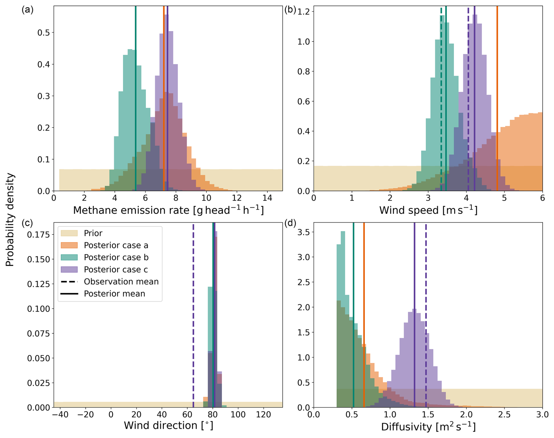
Figure 3Bayesian inference results in the form of posterior distributions obtained using sequential Monte Carlo for the drone flight in the afternoon of 6 March 2024 with 208 heifers. Estimates of (a) methane emission rate, (b) wind speed, (c) wind direction, and (d) diffusivity for three different observation case. Observation case (a) using concentration observations is shown in orange; observation case (b) using concentration observations and mean wind speed data from the drone is shown in green; and observation case (c) using concentration observations and mean wind speed, mean wind direction, and diffusivity data derived from MOST is shown in purple.
In this section, we compare the estimated emission rates derived from the novel Bayesian inference method with those obtained using a conventional mass balance method and IPCC Tier 2 values. A comprehensive overview of the estimated emission rates by the different methods is given in Table B1. Additionally, we evaluate the detection of potential CH4 source locations through hyperspectral satellite observations.
3.1 Source term estimation through drone observations
3.1.1 Bayesian inference method
Figure 3 presents the Bayesian inference results for the drone flight conducted with the heifer herd on the afternoon of 6 March 2024. Results for all drone flights are included in Figs. S25 to S45 and are reported in Table B1. In this section, we analyze the inference results across three observation cases: (a) using only concentration data, (b) combining concentration data with drone-derived wind speed, and (c) incorporating concentration data with mean wind direction, mean wind speed, and diffusivity obtained from MOST. We frequently observe distinct trends when using drone-based methods to estimate CH4 emission rates of sheep and goat herds at Kapiti compared to cattle herds. Except for the camel herd, which consisted of 42 animals, the other herds comprised approximately 100 to 200 animals each (see Table B1). Due to the markedly lower emission rate per individual animal q for sheep and goats, these herds have a lower overall emission rate Q. Consequently, we refer to the sheep and goat herds as “weak(er) sources” to denote their relatively lower emission rates in our study. These observed distinct trends will be discussed in greater detail in this section.
In most of the drone flights, the inferred mean wind direction aligns with the fixed source location and areas of elevated concentration. Overall, the inferred wind direction is both precise and consistent across all three observation cases for cattle drone flights, occasionally overriding the observed wind direction. In Fig. 3, the mean wind direction estimates across the three observation cases coincide, and the inferred direction of 81° corresponds to the angle between the source location and the observation locations with an elevated CH4 mixing ratio shown in Fig. 2. Specifically, the update in wind direction in observation case (a) indicates that our framework can often infer the wind direction solely from the shape of the emission plume and the known source location. The posterior mean wind direction becomes more uncertain when dealing with highly variable wind directions without direct observation (observation case a), such as during the morning flight with camels (Fig. S14) and the morning flight with pregnant does (Fig. S21).
For weak sources, the Bayesian inference algorithm can misinterpret concentration observations as being upwind of a strong emission source rather than downwind from a weak one if no direct wind direction observation is provided. To address this equifinality issue, we used an informed prior bounded by the half wind-rose: °. During the first 2 days of field work, we used a narrower V-shaped flight path instead of the usual half-octagon. Consequently, for the drone flights on these days, marked with a bullet (•) in Table B1, we adjusted the prior to 𝒰(30,135)°. When dealing with weak sources, an informed prior for wind direction was needed in our study to refine the emission rate distribution for observation cases without direct wind direction observations. Even with an informed prior, the posterior distribution of the wind direction can remain relatively uninformed for weak sources, such as weaner kids (Figs. S23 and S24). We note that concentration observations obtained in all locations around the source, such as those from the mass balance flight, can help mitigate this ambiguity.
Wind speed and diffusivity influence the shape of the emission plume. Higher wind speeds elongate the plume, while increased diffusivity broadens it. In observation cases (b) and (c), where direct wind speed observations are available, the posteriors generally align with these observed values. Typically, the wind speed derived from MOST (observation case c) is higher than the wind speed recorded by the drone (observation case b), as demonstrated in Fig. 3. Without direct wind speed observations (observation case a), the Bayesian inference algorithm tends to skew the posterior distribution toward higher wind speeds for most drone flights, as illustrated in Fig. 3. For all drone flights with weak sources, the wind speed posteriors for observation case (a) remain largely uninformed but are slightly skewed toward higher values.
For diffusivity, the posterior distribution in observation case (c) aligns with the direct observation, as shown in Fig. 3. In the absence of observations (observation cases a and b), the diffusivity posterior remains largely uninformed but slightly skewed toward higher values in drone flights with weaker sources as well as for the camel herd. For stronger sources, namely, the cattle herds, the posterior distribution of diffusivity does often shift toward low values, as shown in Fig. 3.
A relationship was observed between the combination of high posterior wind speeds and high posterior diffusivity, resulting in higher estimated emission rates. Higher wind speed and diffusivity indicate a larger plume, both in length and width, suggesting a larger emission rate provided that the concentration observations are the same. The typically higher wind speeds derived from MOST, compared to drone wind speeds, combined with higher posterior diffusivity in observation case (c) compared to observation case (b), generally lead to higher emission rates in observation case (c) compared to observation case (b). This is demonstrated in Fig. 3. The observed relation highlights the importance of reliable wind measurements. We consider observation case (a) the least reliable, as the wind speed estimates often skew toward excessively high values. Observation cases (b) and (c) present an interesting topic for future study: is it more valuable to equip the drone with an anemometer to capture spatial wind variations, albeit potentially affected by the drone's downwash and motion, or to place a fixed anemometer near the source, which may provide more accurate observations and enable a more reliable application of MOST to derive diffusivity data? We hypothesize that a fixed anemometer may be the superior option within the current framework, which employs an advection–diffusion model based on mean wind conditions. In contrast, a mobile sensor may prove superior in frameworks that account for spatial variations in the wind field. Comparing different observing systems in controlled release experiments with a constant and known emission rate can provide further insights into the optimal experimental setup for Bayesian inference observing systems.
Across all drone flights, the emission rate estimates for observation case (c) have a smaller relative uncertainty range compared to observation cases (a) and (b). Specifically, the range is approximately ± 50 % for strong sources and ± 12 % for weak sources, in contrast to ± 65 % and ± 26 % for observation case (a) and ± 55 % and ± 19 % for observation case (b), respectively.
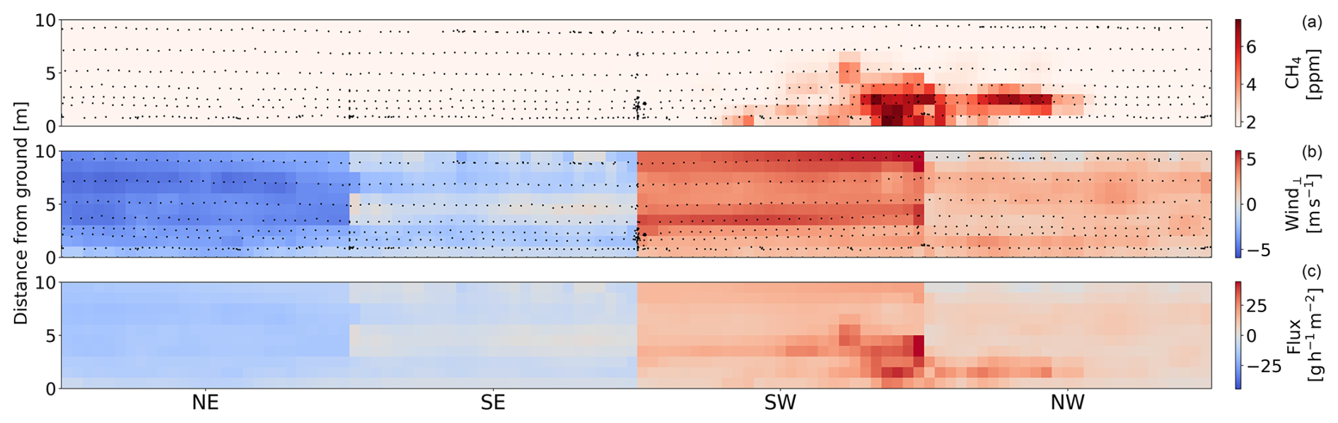
Figure 4Results of the mass balance approach for a drone flight in the afternoon of 6 March 2024 with a herd of 208 heifers. The panels show (a) the interpolated methane mixing ratio measurements, (b) the interpolated perpendicular wind speeds, and (c) the methane fluxes across the vertical sampling planes. Positive (negative) perpendicular wind speeds and fluxes correspond to flow out of (into) the box. The black scatter points indicate the original observation locations.
We compare our estimates to IPCC Tier 1 values to assess their plausibility. It is important to note that IPCC Tier 1 values are highly uncertain, and we do not use these values as a definitive benchmark but rather as a sanity check. Overall, the Bayesian inference emission rate estimates for both strong and weak sources are of the same order of magnitude as the IPCC Tier 1 values: 5.3 g per head per hour for dairy cattle in Africa, 5.3 g per head per hour for camels in developing countries, and 0.6 g per head per hour for sheep and goats in developing countries, with a reported uncertainty range of ± 30 % to ± 50 % (Paustian et al., 2006). Despite large variations in the posterior estimates for wind direction, wind speed, and diffusivity, the emission rate estimates across all observation cases remain plausible when compared to the IPCC Tier 1 values. For example, for the drone flight presented in Fig. 3, the emission rate estimates of 7.2 ± 1.4, 5.4 ± 0.8, and 7.4 ± 0.7 g per head per hour for observation cases (a) to (c), respectively, are considered feasible when compared to the Tier 1 value for dairy cattle in Africa. This underscores the importance of reliable concentration observations, as they alone (observation case a) can provide reasonable emission rate estimates.
Further improvement of the Bayesian inference method could involve extending the sampling duration to more accurately capture the time-averaged plume. Prolonging the sampling time at each observation location may require modifications to the likelihood function. For example, Hutchinson et al. (2019) used a sample duration of 5 s and applied different likelihoods for concentration observations below and above a plume detection threshold. It is important to consider the trade-off between overall sampling duration and the number of sample locations. Investigating this trade-off, along with the formulation of the likelihood function, would be a valuable area for future study to improve the Bayesian inference method for estimating CH4 emission rates. Such optimization could maximize the informational value derived from observations collected with a single battery set.
A promising approach to the information maximization strategy involves the use of autonomous drones that can make in-flight decisions about the optimal sampling path based on real-time observations and previously obtained knowledge. Several studies explore this possibility using reinforcement learning (Loisy and Eloy, 2022; van Hove et al., 2024b). However, these studies often rely on synthetic data, while research involving natural CH4 sources under real-world conditions remains limited. Instead of addressing the information maximization strategy solely on the data collection side, exploring the capabilities of Bayesian hierarchical modeling (Berliner, 2003) to enhance the utilization of information in future research is potentially valuable. The hierarchical Bayesian approach allows information to be shared across drone flights, enabling data to be pooled across, for example, the two heifer drone flights in this study or across all drone flights involving cattle.
3.1.2 Mass balance method
Figure 4 presents the mass balance results of the afternoon drone flight with a herd of heifers, on the same day as the satellite overpass. The panels show the interpolated CH4 mixing ratio measurements (top), perpendicular wind speed (middle), and resulting fluxes (bottom) at the four vertical sampling planes in the NE, SE, SW, and NW directions. The sum of the fluxes in the bottom panel equals the final estimated emission rate for the entire herd Q. The results of the other drone flights are included in Figs. S25 to S45 and Table B1.
Figures 2 and 4 demonstrate the intermittency of the observed instantaneous plume. The CH4 mixing ratios within the plume do not follow a smooth, continuous gradient but instead exhibit an irregular distribution characterized by disconnected patches of elevated mixing ratios. This intermittency complicates the mass balance approach, particularly for drone flights where the signal-to-noise ratio is relatively low. Such conditions include (a) highly variable wind direction or low wind speeds leading to very non-stationary wind conditions (the noise is particularly high) and (b) drone flights with weaker emission sources resulting in low concentration levels (the signal is particularly low), where the variability in the background concentrations and emission plume can considerably affect the accuracy of the emission rate estimate.
The mass balance approach relies on a nonzero horizontal wind to generate a horizontal outflow of CH4 from the imaginary box. Its accuracy improves when the plume morphology remains relatively stable over time. Yang et al. (2018) defines favorable wind conditions as a wind speed greater than 2.3 m s−1 and a steady wind direction with a standard deviation below 33.1°. Measurements collected under wind conditions that do not meet these criteria are marked with a diamond (⧫) in Table B1. These sub-optimal conditions lead to less reliable estimates, as, for example, observed by the negative emission rate of the morning drone flight with camels (Fig. S35). Consequently, these results should be considered unreliable due to unfavorable wind conditions.
Our observations indicate that the estimates for sheep and goats, marked by a triangle (▴) in Table B1, are very variable and inconsistent with the IPCC Tier 1 value of 0.6 g per head per hour (Paustian et al., 2006). Emissions from these smaller animals produce lower CH4 concentration levels, resulting in a lower signal-to-noise ratio when considering the size of the herd. Moreover, for sheep and goats, the emission source and consequently the plume are close to the ground in a region characterized by generally lower wind speeds and complex surface effects caused by, for example, variations in elevation and vegetation. This may increase plume variability, leading to less reliable estimates. Due to these factors, we consider the mass balance estimates for drone flights with sheep and goats unreliable. The mass balance estimates for cattle are more plausible, as they are of the same order of magnitude as the IPCC Tier 1 value of 5.3 g per head per hour for dairy cattle in Africa (Paustian et al., 2006). While these Tier 1 values can provide a rough reference point, they should not be interpreted as exact estimates of CH4 emissions. The negative emission rate for camels in the morning is unrealistic, but the estimate in the afternoon is within a similar range as the IPCC Tier 1 value of 5.3 g per head per hour (Paustian et al., 2006).
To mitigate the effect of plume variability over time, several studies have conducted repeated drone flights (Gålfalk et al., 2021; Andersen et al., 2021). This approach can yield a more robust approximation of the emission rate by averaging the estimates from multiple drone flights, thereby reducing – though not eliminating – uncertainty due to temporal variability. In a single drone flight, capturing the time-averaged plume can potentially be improved by increasing the number of plume observations relative to background observations. Several studies, particularly larger-scale experiments using airplanes, conduct flights along a single vertical sampling plane downwind from the prevailing wind direction (Allen et al., 2019; Cambaliza et al., 2014). The term ci,j in Eq. (6) is then replaced by , where c0 is the estimated background concentration. However, this sampling approach introduces uncertainty due to the estimation of the background concentration, the variability of which must be accounted for in the overall uncertainty estimate.
Although onboard wind measurements with a sonic anemometer are considered ideal (Allen et al., 2019), practical constraints have necessitated the use of nearby weather stations for wind data in several studies (Allen et al., 2019; Nathan et al., 2015). Morales et al. (2022) demonstrated, through controlled release experiments, that using wind data from an anemometer close to the source, which captures changing wind conditions during the flight, is more accurate than applying a wind profile through MOST (Eq. A1) that only accounts for wind speed variation with altitude. Given that we did not have an anemometer available on the drone, using corrected wind speeds from the flight controller was our best available option. An onboard anemometer could reduce measurement uncertainty of the instantaneous wind field, but it does not reduce uncertainty due to temporal uncertainty.
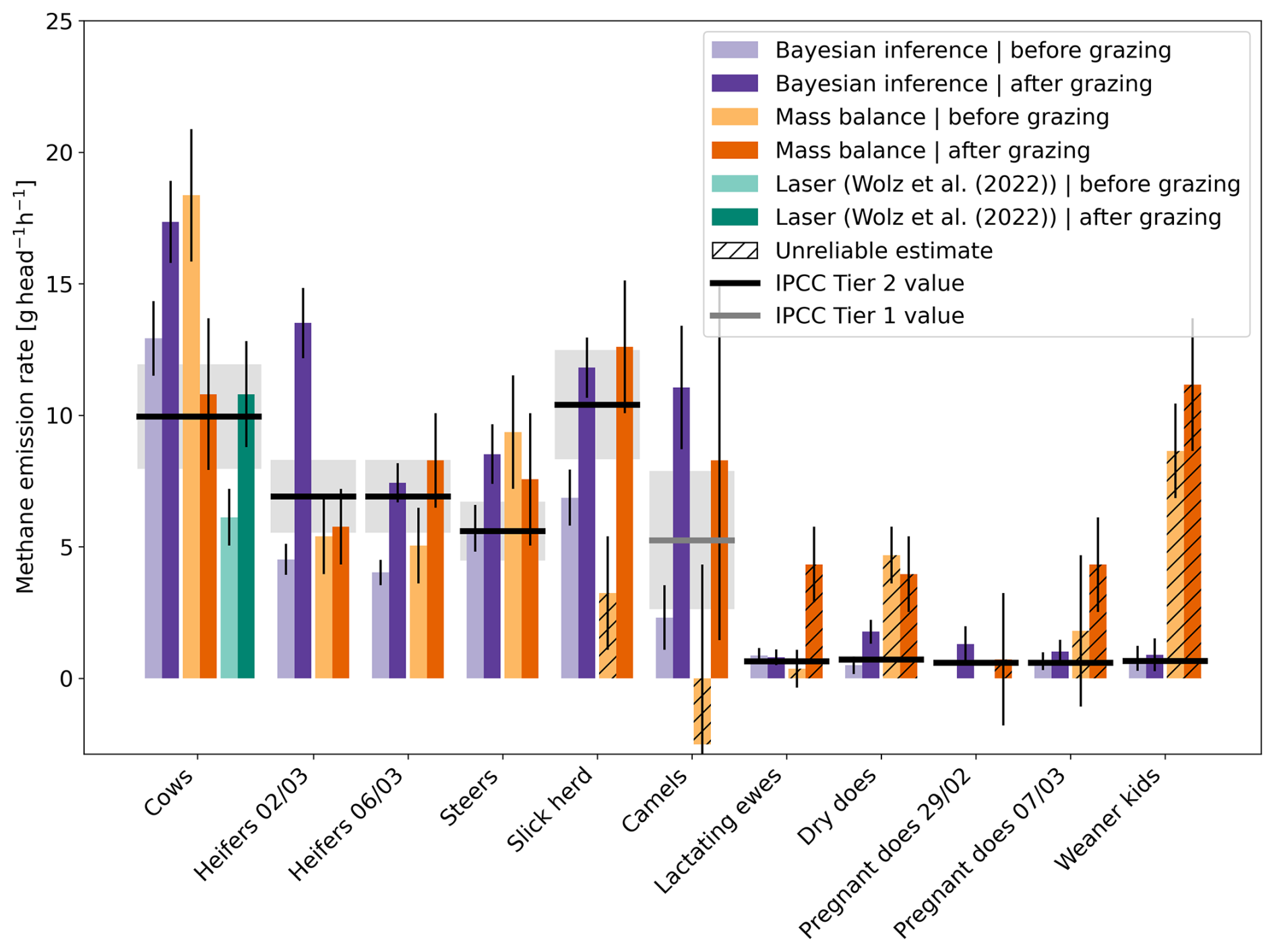
Figure 5Methane emission rate estimates from the Bayesian inference method using concentration observations and mean wind speed, mean wind direction, and diffusivity data derived from Monin–Obukhov similarity theory (observation case c), the mass balance approach, a laser spectrometry study by Wolz et al. (2022), and IPCC emission factors converted from daily to hourly emission rates. Error bars represent one standard deviation uncertainty. The uncertainty range of IPCC values, depicted by gray shading, is ± 20 % for Tier 2 values and ± 30 % to ± 50 % for Tier 1 values (Paustian et al., 2006); this figure uses ± 50 % for the IPCC Tier 1 value. Unreliable mass balance estimates due to a low signal-to-noise ratio are indicated by hatched lines.
3.2 Method comparison
In this section, we evaluate the CH4 emission rate results obtained through Bayesian inference by comparing them with results from other methods and literature values. Figure 5 presents the Bayesian inference results for observation case (c) alongside estimates from the mass balance approach, a laser spectrometry study previously conducted at Kapiti by Wolz et al. (2022), and IPCC emission values.
In Sect. 3.1.1 and 3.1.2, we found that the Bayesian inference results for all herds are of the same order of magnitude as the IPCC Tier 1 values. In contrast, our mass balance results for strong sources (cattle herds) fall within the same order of magnitude as the IPCC Tier 1 values, while those for weak sources (sheep and goat herds) are substantially higher than the IPCC Tier 1 values in several drone flights. This finding was further supported by comparison to the herd-specific IPCC Tier 2 values, which are generally regarded as more reliable, though they should not be considered definitive. We compared the average (pre- and post-grazing) emission rate estimates to the IPCC Tier 2 values. We found a mean relative difference of 16 % for the Bayesian inference results and a mean relative difference of 10 % for the mass balance results across flights with strong sources of Q≈ 700 g h−1 to Q≈ 1,500 g h−1 (Table B1). For the flights with weaker sources of Q≈ 70 g h−1 to Q≈ 140 g h−1 (Table B1), we observed a mean relative difference of 40 % for the Bayesian inference results and a mean relative difference of 683 % for the mass balance results. This disparity suggests that the source term estimation threshold of the Bayesian inference method is lower than that of the mass balance method applied in our study. Consequently, Bayesian inference may be more effective in estimating weaker sources, where the mass balance method may provide unreliable estimates.
We compare the Bayesian inference estimates to results from previous studies conducted at Kapiti. Our average (pre- and post-grazing) emission rate estimate for steers was 7.1 ± 0.7 g per head per hour, which aligns with a respiration chamber experiment showing emission rates ranging from 6.7 to 7.7 g per head per hour depending on diet (Korir et al., 2022b). Our average emission rate estimate for lactating ewes was 0.8 ± 0.2 g per head per hour, which overlaps with the emission rate for sheep ranging from 0.6 to 0.8 g per head per hour found in a respiration chamber experiment (Mwangi et al., 2023). Our estimate is on the higher end, which is expected as emissions from lactating animals are generally larger than those from non-lactating animals due to their increased feed intake to meet the energy demands of milk production (Broucek, 2014). In another respiration chamber experiment, the estimated emission rates from cows ranged from 7.6 to 11.3 g per head per hour depending on diet (Korir et al., 2022a). In contrast, our average estimate was notably higher at 15.2 ± 1.0 g per head per hour.
Wolz et al. (2022) utilized open-path laser spectroscopy with backward Lagrangian stochastic dispersion modeling to estimate nighttime CH4 emissions from a mixed cattle herd across 14 nights in September and October 2019. The resulting mean emission rates Q were normalized to the equivalent weight of a cow to obtain q for a hypothetical cow herd, rather than normalizing by the number of animals to obtain q for the observed mixed cattle herd. Figure 5 shows the results obtained at 09:00 East Africa Time (EAT), before grazing, and at 00:30 EAT, after grazing. Note that the latter nocturnal measurements were obtained later than our drone flights, which were conducted in the afternoon. We observe that our Bayesian inference results for cows are higher, both before and after grazing, compared to estimates from Wolz et al. (2022). This difference could be due to an overestimation by the Bayesian inference method, or the emission rate might have been this high at the times of the drone flights. Wolz et al. (2022) reported a mean emission rate over 14 repeated experiments, whereas the Bayesian inference result is an estimate based on a single drone flight. Additionally, differences in methodology, differences in the timing of the measurements, and the herd weight normalization used by Wolz et al. (2022) could contribute to the discrepancies. Both studies were conducted at the end of a dry season; however, our field campaign was conducted during a normal dry season, whereas the dry season studied by Wolz et al. (2022) was extreme. The severity of this dry season likely affected feed intake and feed quality, potentially reducing CH4 emission rates.
No camel studies have previously been conducted in Kapiti, so we compared our Bayesian inference results for camels to those of a respiration chamber experiment conducted in Australia by Dittmann et al. (2014). This study estimated a CH4 emission rate of 4.0 g per head per hour for Bactrian camels fed exclusively on alfalfa. Our average (pre- and post-grazing) estimate is higher at 6.7 ± 1.3 g per head per hour. Note that the studies involve different camel species and diets. We emphasize that the number of experiments conducted with camels and the extent of current knowledge are minimal and that further research is required to gain more insight into the emissions of CH4 from camels. Based on Bayesian inference, we observe a larger increase in estimated CH4 production after grazing in camels compared to cattle. Replication of this result through repeated experiments would be a promising avenue for further research.
Feeding is known to increase CH4 production in ruminants (Amon et al., 2001; Hegarty, 2013). Using a one-sided Student's t-test (Student, 1908) on the relative difference in emissions pre- and post-grazing across all animal groups, we found a statistically significant effect of grazing for the Bayesian inference results (p-value = 0.009) but not for the mass balance results (p-value = 0.194). We observe that 7 out of 10 Bayesian inference cases have markedly higher mean emission rates in the afternoon compared to the morning. For pregnant does and weaner kids, while the emission estimates increase after grazing, considerable overlap in the uncertainty ranges makes the effect ambiguous. In the case of lactating ewes, the difference in emissions before and after grazing is only slightly negative and also ambiguous. In contrast, the mass balance results do not consistently demonstrate an increase in CH4 emissions post-grazing, with substantial increases observed in only 2 out of 10 cases: the slick herd and lactating ewes. We consider this to be a promising indicator for the greater reliability and accuracy of our Bayesian inference results compared to our mass balance results.
One advantage of using the Bayesian inference method over the IPCC Tier 2 approach is the ability to estimate diurnal variations, which allows us to observe the effects of feeding. Additionally, the uncertainty in the Bayesian inference results can typically be reduced by assimilating a larger dataset, suggesting that repeated drone flights can yield more reliable results (Pirk et al., 2022). Deriving IPCC Tier 2 values is time-consuming due to the measurement of live weight and live weight changes of individual animals, and considerable unquantified uncertainty remains in our ability to estimate the feed intake of animals in pastoral systems like at Kapiti. Furthermore, the accuracy of the method relies partly on the accuracy of the methane conversion factor Ym, which is determined based on previous research and may not be representative of the specific animals being studied.
In comparison to the Bayesian inference method, the mass balance approach is more straightforward to use due to its smaller model complexity, which requires less coding and reduces the need for parameter tuning. However, based on this study, Bayesian inference results can be more reliable, as demonstrated by the consistent observation of increased emissions post-grazing, as shown in Fig. 5. In both the mass balance method and the Bayesian inference method, we use a sensor – a drone – to capture snapshots of a non-stationary emission plume. However, the physical models of both methods – Eq. (1) for our Bayesian inference approach and Eq. (6) for the mass balance method – are based on the assumption of a statistically stationary plume. A conceptual difference between the two methods lies in how they handle the discrepancy between the turbulent (instantaneous) observations acquired by the drone and the mean concentration and mean wind field represented in the model. The Bayesian inference method explicitly accounts for this discrepancy through observation error R, while the mass balance approach does not explicitly address this inconsistency. Instead, we account for this violation only implicitly by including a temporal variation term within the uncertainty range of the mass balance estimates. We observed that the mass balance approach estimates are sensitive to low signal-to-noise levels, making the resulting estimates of weaker sources and under highly variable wind conditions unreliable. In contrast, the Bayesian inference method proved to be more robust in estimating weaker sources and under variable wind conditions. This robustness may be attributed to explicitly accounting for discrepancies between instantaneous observations and the assumed stationarity of the concentration and wind fields in the physical model.
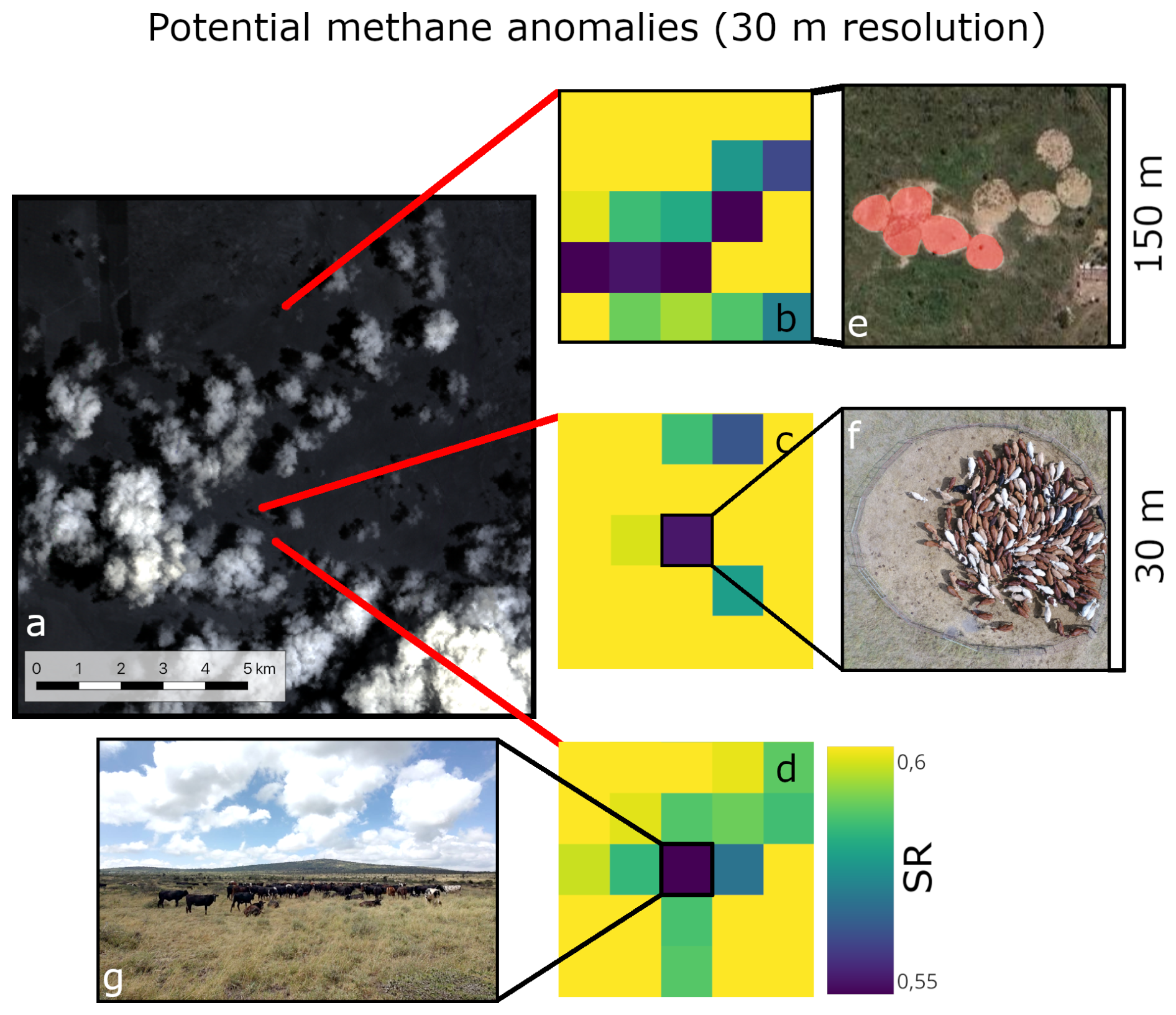
Figure 6(a) PRISMA true color image of Kapiti from 6 March 2024 08:00 Coordinated Universal Time (UTC) + 3 h, corresponding to East Africa Time. (b) to (d) The simple ratio (SR) radiance index of 2300/2100 nm with 30 m resolution for three distinct sites: (e) five adjacent bomas (shaded red) housing 583 cows at the time of the satellite overpass but empty in this picture, (f) a single boma at the drone field site with 206 heifers, and (g) a free-grazing herd of 148 heifers. (e) includes ©Google Satellite Imagery (2021). PRISMA product derived from L1 6 March 2024©Italian Space Agency (ASI) (2024). All rights reserved.
3.3 Source detection through satellite observations
Figure 6 shows a true color image of a part of Kapiti, captured by the PRISMA satellite on 6 March 2024. Despite the partly cloudy conditions, the irregular cloud cover did not occlude the satellite observations of all three cattle herds within our study area. The maps in Fig. 6b to Fig. 6d show the SR index for a region of 5 pixels by 5 pixels with a spatial resolution of 30 m across three different sites: five adjacent bomas housing 583 cows (Fig. 6e), the boma at the drone field site with 206 heifers (Fig. 6f), and a free-grazing herd of 148 heifers (Fig. 6g).
We observed a lower SR index at the herd locations compared to the surrounding background. Specifically, we detected anomalies with the two herds inside a boma against a bare soil background, as well as the free-grazing herd against a green vegetation background. These SR anomalies, which indicate relatively low radiance levels in the CH4 absorption feature, may suggest higher atmospheric CH4 concentrations, pointing to the presence of a CH4 source. However, because the estimated emission rates of the herds are well below the expected detection limits for point sources from PRISMA of approximately 500 kg h−1 (Guanter et al., 2021), caution should be taken in interpreting this result. Importantly, this lower SR level may also arise from features associated with grazing or the herd's presence, such as changes in vegetation cover or soil disturbance. Although our limited dataset prevents us from evaluating whether the observed anomalies are related to emissions or landscape features, these preliminary results call for more in-depth investigation of the proposed approach for detecting the location of potential CH4 sources using last-generation high-resolution hyperspectral satellite missions. Further dedicated studies are necessary to evaluate the generalizability of these findings.
The use of hyperspectral satellite data for detecting potential CH4 source locations marks an initial step toward mapping regional CH4 emissions. By identifying areas of interest, we can strategically target drone campaigns to investigate these potential source locations. In our study focused on ruminant herds, the source locations were already known. However, detecting potential source locations from satellite imagery can be particularly useful in regions such as thawing permafrost landscapes, where CH4 source locations are typically unknown.
3.4 Bayesian lessons learned
Here, we share our experiences in quantifying CH4 emissions using Bayesian inference with drone and flux tower observations, with the aim of advancing local source term estimation through Bayesian inference.
-
Rather than treating the herd as a single point source, we modeled it as a set of sources with equal strengths, which we found to be more accurate. Modeling the herd as a single point source led to higher inferred mean diffusivity in most drone flights due to the large horizontal spread of instantaneous observed elevated concentrations above the background level.
-
We assumed the set of source locations to be fixed known parameters. When treated as an unknown parameter, the posterior distribution for source location broadened along the prevailing wind direction and increased the uncertainty in the emission rate estimates. This can be attributed to equifinality: a stronger source further away can produce a similar concentration observation to that of a weaker source nearby. Incorporating concentration data collected around the source enhanced the accuracy of source location posteriors. We tested this by incorporating the observations of the mass balance flights.
-
We observed equifinality across multiple parameter combinations, implying that incorporating observations related to unknown parameters is beneficial and may even be necessary to adequately constrain their probability distributions. While wind direction can be effectively constrained using concentration observations alone, wind speed measurements – such as those from the drone or flux tower – considerably enhance the inference process. Further research is recommended to identify the most reliable observational platform for this purpose. Diffusivity proved difficult to constrain based on instantaneous concentration observations alone, but we observed that diffusivity observations derived from eddy-covariance data helped to constrain the diffusivity probability distribution.
-
We restricted the uniform prior for wind direction to a half wind-rose aligned with the prevailing wind direction. Using the entire wind-rose introduced ambiguity between upwind observations of strong sources and downwind observations of weak sources, specifically in drone flights with herds of sheep and goats. Incorporating concentration observations around the source can help mitigate this ambiguity.
-
Treating the background concentration as a known parameter was necessary in this study because the Bayesian inference algorithm struggled to infer reliable estimates in several drone flights when this parameter was considered unknown, leading to unreliable emission rate inferences. The algorithm struggled to distinguish between background and elevated concentrations without relying on this assumption. We anticipate that using concentration observations obtained over longer sampling times, with an adjusted likelihood function, could potentially address this issue.
-
The biggest challenge in setting up the Bayesian framework was the mismatch between instantaneous concentration observations and the time-averaged dispersion model, which complicated the design of the likelihood function. A broad Gaussian likelihood proved effective. Still, we recommend further investigation into the likelihood design, in combination with extended sampling times to better capture the time-averaged emission plume. However, longer sampling times reduce the number of locations that can be observed on a single drone battery charge. This limitation makes intelligent sampling path design a promising topic for further study.
In our study conducted in Kenya, we leveraged drone and flux tower observations alongside a Bayesian inference approach to estimate CH4 emissions from ruminants – an important, yet poorly understood, contributor to the global CH4 emission inventory. Furthermore, we showed that anomalies detected in the SWIR spectrum of hyperspectral satellite data may indicate the presence of CH4 sources.
4.1 Insights into CH4 emission detection and estimation from ruminants
Using drone observations, we estimated the CH4 emission rates of various ruminant herds – including cattle (cows, heifers, steers, and slick herd), sheep (lactating ewes), goats (dry does, pregnant does, and weaner kids), and camels – applying both Bayesian inference and mass balance methods. Due to low signal-to-noise levels, the mass balance method did not consistently provide reliable estimates for weaker sources, such as the sheep and goat herds. However, under favorable wind conditions, we estimated cattle herd emissions ranging between 700 and 1500 g h−1. In contrast, the Bayesian inference method performed better for weaker sources, estimating sheep and goat herd emissions in the range of 70–140 g h−1, while it was effective for the different cattle and camel herds as well. We observed the hypothesized increase in CH4 production following feeding in the majority of Bayesian inference drone flights, whereas this effect was much less discernible in the mass balance flights. Additionally, the Bayesian inference method results appeared less affected by variable wind conditions, further suggesting its superior performance over the mass balance method in this study.
Overall, the Bayesian inference results aligned with the IPCC Tier 2 emission values, indicating compatibility without implying mutual validation. The method's benefits lie in its ability to estimate temporal variations in CH4 production, as well as its capacity to assimilate observations from various measurement platforms while incorporating their uncertainties. The robust performance of the Bayesian inference approach in this case study, estimating diverse CH4 source strengths under various atmospheric conditions, underscores its potential as a valuable tool for estimating CH4 emissions in agricultural systems and other landscapes.
In an exploratory analysis, we detected anomalies in the SWIR spectrum from hyperspectral satellite data associated with two cattle herds on bare soil and one herd on grassland, which were emitting approximately 1000 g h−1. While this detection is promising for mapping CH4 emissions, we must be cautious in interpreting the results, as the expected detection limit is 500 kg h−1 Guanter et al. (2021). Further research is needed to ascertain whether these anomalies correlate directly with increased CH4 concentrations or if they stem from other features related to the herd's presence or grazing activities. Ultimately, the ability to identify potential emission plumes from hyperspectral data anomalies – especially from relatively low-emission sources like those in our study – represents a promising initial step toward mapping regional CH4 emissions in landscapes where the precise source locations are unknown.
4.2 Future applications
Future applications of the Bayesian framework for source term estimation could extend to diverse natural and anthropogenic sources, including CH4 emissions from wetlands, thawing permafrost, landfills, and wastewater disposal sites. Our ultimate aim is to leverage Bayesian inference to comprehensively map these areas, thereby improving our understanding of spatial variations in emissions across diverse landscapes. While the framework is readily applicable to point-like sources, such as thermokarst hotspots, future research should focus on adapting this framework to infer emissions from landscapes characterized by multiple sparse sources that may vary in size and produce overlapping emission plumes. This adaptation may require not only precise estimation of emission rates but also accurate localization of these sources.
In regions where observational data are sparse, the Bayesian inference method can be employed using a gas sensor and an anemometer mounted on the drone or positioned near the source. This approach could eliminate the need for a nearby flux tower, making the observing framework suitable for remote sites. Conversely, in observation-rich environments, the Bayesian inference method can integrate data from multiple observation platforms. For example, data obtained from laser spectrometry or observations from multiple drones can be assimilated to improve the accuracy of emission estimates.
Overall, the insights gained from our study demonstrate the potential of Bayesian inference methods, combined with drone and flux tower observations, for enhancing our understanding of CH4 emissions at local scales, thereby contributing to the improvement of CH4 inventories and mitigation studies.
Obukhov length L [m] is positive in stable atmospheric conditions and negative in unstable atmospheric conditions. During all drone flights, the atmosphere was unstable. We use Monin–Obukhov similarity theory (MOST; see Stull, 1989; Hanna et al., 1982) to estimate the vertical profile of the mean wind speed V(z) [m s−1] and mean eddy diffusivity K(z) [m2 s−1], where z is the distance above the ground.
Under unstable atmospheric conditions, the mean wind speed profile is estimated by
where u∗ is the friction velocity, κ=0.4 is the von Kármán constant, and z0 [m] is the aerodynamic roughness length. We use z0 = 0.05 m, which corresponds to terrain with long grass and few trees (Stull, 1989), and a displacement height of d = 0.10 m. The dimensionless wind shear ΦM is approximated by
The resulting mean wind speed at the height of the sonic anemometer on the flux tower qualitatively matches the mean wind speeds measured by the same sonic anemometer (Fig. S3).
The eddy diffusivity for effectively passive tracers such as CH4 is generally assumed to be equal to the eddy diffusivity for heat. The mean eddy diffusivity profile is given by
where ΦH is the dimensionless potential temperature gradient. For unstable atmospheric conditions, it is assumed to be given by
Table B1Overview of methane emission rate estimates obtained by the mass balance method, the Bayesian inference method, and the IPCC Tier 2 workflow with a ± 20 % uncertainty range (Paustian et al., 2006). The cases are defined as follows: (a) using concentration observations; (b) using concentration observations and mean wind speed data from the drone; and (c) using concentration observations and mean wind speed, mean wind direction, and diffusivity data derived from Monin–Obukhov similarity theory. Emission rate estimates are given in q [], where hd is short for head, except for the last column, which presents estimates in Q [g h−1], i.e., for the entire herd. One standard deviation uncertainty is reported. AM and PM indicate drone flights conducted in the morning before feeding and in the afternoon after feeding, respectively. Wind speed (VEC [m s−1]) and wind direction (ϕEC [°]) data are from the flux tower during the mass balance flight. Further notation: (⧫) unreliable drone flight results due to unfavorable wind conditions (following Yang et al., 2018); (▴) unreliable estimates due to a low signal-to-noise ratio caused by a weak emission source; (•) estimates using a narrower prior for wind direction, i.e., 𝒰(30,135); and (★) IPCC Tier 1 value with a ± 50 % uncertainty range (Paustian et al., 2006).
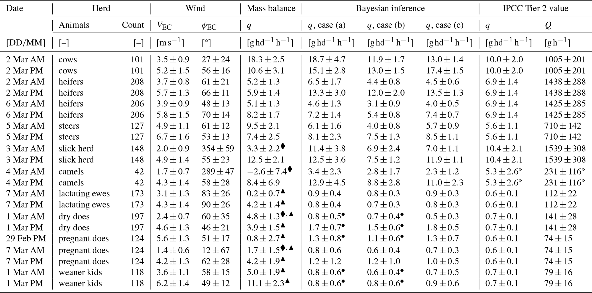
The drone and flux tower dataset, along with the digital elevation model of Kapiti, can be accessed from https://doi.org/10.5281/zenodo.14214699 (van Hove et al., 2024a). The data processing scripts are available at https://github.com/AlouetteUiO/MIK (van Hove, 2024c). The prismaread package for processing PRISMA satellite data is available at https://doi.org/10.5281/zenodo.4019081 (Busetto, 2020).
The supplement related to this article is available online at https://doi.org/10.5194/bg-22-4163-2025-supplement.
Conceptualization: AvH, NP, KA. Methodology: AvH, KA, NP. Software: AvH. Formal analysis: AvH (drone-based methods), VL (IPCC Tier 2 values), RC (satellite data). Investigation: AvH and JH (drone flights), VO (eddy-covariance data), RC and FF (satellite data). Resources: CA (host at Kapiti and coordination field campaign). Writing – Original Draft: AvH. Writing – Review and Editing: KA, NP, VL, CA, RC, VO, FF, AvH. Visualization: AvH, RC (Fig. 6). Funding acquisition: VL, NP, CA, FF.
The contact author has declared that none of the authors has any competing interests.
The content of this article is the sole responsibility of the authors and does not necessarily reflect the views of the European Union.
Publisher's note: Copernicus Publications remains neutral with regard to jurisdictional claims made in the text, published maps, institutional affiliations, or any other geographical representation in this paper. While Copernicus Publications makes every effort to include appropriate place names, the final responsibility lies with the authors.
We would like to thank Ilona Gluecks from ILRI for providing information about the different ruminant herds at Kapiti and Endale Balcha Gurmu from ILRI for assisting with the IPCC Tier 2 workflow. Furthermore, we would like to thank Nehemiah Kimengich, Nelson Kipchirchir, and Elly Kibira at Kapiti for their assistance in the field. We would also like to thank Lutz Merbold for his contribution to the flux tower data. Moreover, we would like to thank Luc Girod from UiO for his help with drone imagery processing. This study contains modified data of the PRISMA satellite of ESA – Agenzia Spaziale Italiana (ASI) (Year 2024). We would like to thank Monica Pepe from CNR and Patrizia Sacco from ASI for the data procurement.
This research has been supported by the Norges Forskningsråd (grant nos. 333232 and 301552) and the European Research Council, HORIZON EUROPE European Research Council (grant no. 101116083). This work was supported by the Research Council of Norway (projects #333232 (CircAgric-GHG) and #301552 (Spot-On)) and the European Research Council (project #101116083 (ACTIVATE)). This work is a contribution to the strategic research initiative LATICE (#UiO/GEO103920), the Center for Biogeochemistry in the Anthropocene, as well as the Center for Computational and Data Science at the University of Oslo. This study was supported by the CGIAR Initiatives Livestock and Climate and Mitigate+: Low-Emission Food Systems, which are supported by contributors to the CGIAR Trust Fund. This work was supported by the European Union through the EU-DeSIRA ESSA project (Earth observation and environmental sensing for climate-smart sustainable agropastoralism ecosystem transformation in East Africa).
This paper was edited by Ji-Hyung Park and reviewed by Ji-Hyung Park and one anonymous referee.
Abichandani, P., Lobo, D., Ford, G., Bucci, D., and Kam, M.: Wind Measurement and Simulation Techniques in Multi-Rotor Small Unmanned Aerial Vehicles, IEEE Access, 8, 54910–54927, https://doi.org/10.1109/ACCESS.2020.2977693, 2020. a
Allen, G., Hollingsworth, P., Kabbabe, K., Pitt, J. R., Mead, M. I., Illingworth, S., Roberts, G., Bourn, M., Shallcross, D. E., and Percival, C. J.: The development and trial of an unmanned aerial system for the measurement of methane flux from landfill and greenhouse gas emission hotspots, Waste Manage., 87, 883–892, https://doi.org/10.1016/j.wasman.2017.12.024, 2019. a, b, c, d
Amon, B., Amon, T., Boxberger, J., and Alt, C.: Emissions of NH3, N2O and CH4 from dairy cows housed in a farmyard manure tying stall (housing, manure storage, manure spreading), Nutr. Cycl. Agroecosys., 60, 103–113, https://doi.org/10.1023/A:1012649028772, 2001. a, b, c
Andersen, T., Vinkovic, K., De Vries, M., Kers, B., Necki, J., Swolkien, J., Roiger, A., Peters, W., and Chen, H.: Quantifying methane emissions from coal mining ventilation shafts using an unmanned aerial vehicle (UAV)-based active AirCore system, Atmospheric Environment: X, 12, 100135, https://doi.org/10.1016/j.aeaoa.2021.100135, 2021. a, b, c, d, e, f
Anderson, G.: Error propagation by the Monte Carlo method in geochemical calculations, Geochim. Cosmoch. Acta, 40, 1533–1538, https://doi.org/10.1016/0016-7037(76)90092-2, 1976. a
Arndt, C., Leytem, A., Hristov, A., Zavala-Araiza, D., Cativiela, J., Conley, S., Daube, C., Faloona, I., and Herndon, S.: Short-term methane emissions from 2 dairy farms in California estimated by different measurement techniques and US Environmental Protection Agency inventory methodology: A case study, J. Dairy Sci., 101, 11461–11479, https://doi.org/10.3168/jds.2017-13881, 2018. a, b, c, d
Bai, M., Velazco, J. I., Coates, T. W., Phillips, F. A., Flesch, T. K., Hill, J., Mayer, D. G., Tomkins, N. W., Hegarty, R. S., and Chen, D.: Beef cattle methane emissions measured with tracer-ratio and inverse dispersion modelling techniques, Atmos. Meas. Tech., 14, 3469–3479, https://doi.org/10.5194/amt-14-3469-2021, 2021. a
Baldwin, R., McLeod, K., Klotz, J., and Heitmann, R.: Rumen Development, Intestinal Growth and Hepatic Metabolism In The Pre- and Postweaning Ruminant, J. Dairy Sci., 87, E55–E65, 2004. a
Banner, K. M., Irvine, K. M., and Rodhouse, T. J.: The use of Bayesian priors in Ecology: The good, the bad and the not great, Methods Ecol. Evol., 11, 882–889, https://doi.org/10.1111/2041-210X.13407, 2020. a
Berliner, L. M.: Physical-statistical modeling in geophysics, J. Geophys. Res., 108, 8776, https://doi.org/10.1029/2002JD002865, 2003. a
Borchardt, J., Gerilowski, K., Krautwurst, S., Bovensmann, H., Thorpe, A. K., Thompson, D. R., Frankenberg, C., Miller, C. E., Duren, R. M., and Burrows, J. P.: Detection and quantification of CH4 plumes using the WFM-DOAS retrieval on AVIRIS-NG hyperspectral data, Atmos. Meas. Tech., 14, 1267–1291, https://doi.org/10.5194/amt-14-1267-2021, 2021. a
Broucek, J.: Production of Methane Emissions from Ruminant Husbandry: A Review, J. Environ. Prot., 05, 1482–1493, https://doi.org/10.4236/jep.2014.515141, 2014. a, b
Brown, L. R., Benner, D. C., Champion, J. P., Devi, V. M., Fejard, L., Gamache, R. R., Gabard, T., Hilico, J. C., Lavorel, B., Loete, M., Mellau, G. C., Nikitin, A., Pine, A. S., Predoi-Cross, A., Rinsland, C. P., Robert, O., Sams, R. L., Smith, M. A., Tashkun, S. A., and Tyuterev, V. G.: Methane line parameters in HITRAN, J. Quant. Spectrosc. Ra., 82, 219–238, https://doi.org/10.1016/S0022-4073(03)00155-9, 2003. a
Burba, G.: Eddy Covariance Method for Scientific, Industrial, Agricultural and Regulatory Applications: A Field Book on Measuring Ecosystem Gas Exchange and Areal Emission Rates, LI-COR Beosciences, https://doi.org/10.13140/RG.2.1.4247.8561, 2013. a
Burgués, J. and Marco, S.: Environmental chemical sensing using small drones: A review, Sci. Total Environ., 748, 141172, https://doi.org/10.1016/j.scitotenv.2020.141172, 2020. a
Busetto, L.: lbusett/prismaread: v1.0.0, Zenodo [code], https://doi.org/10.5281/zenodo.4019081, 2020. a, b
Calder, K. L.: Multiple-source plume models of urban air pollution—their general structure, Atmos. Environ., 11, 403–414, 1977. a
Cambaliza, M. O. L., Shepson, P. B., Caulton, D. R., Stirm, B., Samarov, D., Gurney, K. R., Turnbull, J., Davis, K. J., Possolo, A., Karion, A., Sweeney, C., Moser, B., Hendricks, A., Lauvaux, T., Mays, K., Whetstone, J., Huang, J., Razlivanov, I., Miles, N. L., and Richardson, S. J.: Assessment of uncertainties of an aircraft-based mass balance approach for quantifying urban greenhouse gas emissions, Atmos. Chem. Phys., 14, 9029–9050, https://doi.org/10.5194/acp-14-9029-2014, 2014. a, b, c
Chopin, N.: A sequential particle filter method for static models, Biometrika, 89, 539–552, https://doi.org/10.1093/biomet/89.3.539, 2002. a
Chopin, N. and Papaspiliopoulos, O.: An Introduction to Sequential Monte Carlo, 1st edition 2020 edn., Springer Series in Statistics, Springer Nature, Cham, https://doi.org/10.1007/978-3-030-47845-2, 2020. a, b, c
Crazzolara, C., Ebner, M., Platis, A., Miranda, T., Bange, J., and Junginger, A.: A new multicopter-based unmanned aerial system for pollen and spores collection in the atmospheric boundary layer, Atmos. Meas. Tech., 12, 1581–1598, https://doi.org/10.5194/amt-12-1581-2019, 2019. a
Cusworth, D. H., Bloom, A. A., Ma, S., Miller, C. E., Bowman, K., Yin, Y., Maasakkers, J. D., Zhang, Y., Scarpelli, T. R., Qu, Z., Jacob, D. J., and Worden, J. R.: A Bayesian framework for deriving sector-based methane emissions from top-down fluxes, Communications Earth & Environment, 2, 242, https://doi.org/10.1038/s43247-021-00312-6, 2021. a
Daube, C., Conley, S., Faloona, I. C., Arndt, C., Yacovitch, T. I., Roscioli, J. R., and Herndon, S. C.: Using the tracer flux ratio method with flight measurements to estimate dairy farm CH4 emissions in central California, Atmos. Meas. Tech., 12, 2085–2095, https://doi.org/10.5194/amt-12-2085-2019, 2019. a
Dittmann, M. T., Runge, U., Lang, R. A., Moser, D., Galeffi, C., Kreuzer, M., and Clauss, M.: Methane Emission by Camelids, PLOS ONE, 9, e94363, https://doi.org/10.1371/journal.pone.0094363, 2014. a, b
Dogniaux, M., Maasakkers, J. D., Varon, D. J., and Aben, I.: Report on Landsat 8 and Sentinel-2B observations of the Nord Stream 2 pipeline methane leak, Atmos. Meas. Tech., 17, 2777–2787, https://doi.org/10.5194/amt-17-2777-2024, 2024. a
Doucet, A. and Johansen, A. M.: A tutorial on particle filtering and smoothing: fiteen years later, in: The Oxford handbook of nonlinear filtering, Oxford handbooks in mathematics, edited by: Crisan, D. and Rozovskii, B. Oxford, N.Y, Oxford University Press, 656–705 pp., ISBN 9780199532902, 2009. a
Evangeliou, N., Thompson, R. L., Eckhardt, S., and Stohl, A.: Top-down estimates of black carbon emissions at high latitudes using an atmospheric transport model and a Bayesian inversion framework, Atmos. Chem. Phys., 18, 15307–15327, https://doi.org/10.5194/acp-18-15307-2018, 2018. a
Francis, A., Li, S., Griffiths, C., and Sienz, J.: Gas source localization and mapping with mobile robots: A review, J. Field Robot., 39, 1341–1373, https://doi.org/10.1002/rob.22109, 2022. a
Gålfalk, M., Nilsson Påledal, S., and Bastviken, D.: Sensitive Drone Mapping of Methane Emissions without the Need for Supplementary Ground-Based Measurements, ACS Earth Space Chem., 5, 2668–2676, https://doi.org/10.1021/acsearthspacechem.1c00106, 2021. a, b, c, d, e
Gavrilova, O., Leip, A., Dong, H., Macdonald, J., Gomez, C., Amon, B., Barahona Rosales, R., Agustin, Del Prado, A., Lima, M., Oyhantcabal, W., Weerden, T., Widiawati, Y., Bannink, A., Beauchemin, K., Clark, H., Leytem, A., Kebreab, E., Ngwabie, N., and Vellinga, T.: Emissions from livestock and manure management, in: 2019 Refinement to the 2006 IPCC Guidelines for National Greenhouse Gas Inventories, IPCC, 2019. a
Giardino, C., Bresciani, M., Braga, F., Fabbretto, A., Ghirardi, N., Pepe, M., Gianinetto, M., Colombo, R., Cogliati, S., Ghebrehiwot, S., Laanen, M., Peters, S., Schroeder, T., Concha, J. A., and Brando, V. E.: First evaluation of prisma level 1 data for water applications, Sensors (Switzerland), 20, 1–16, https://doi.org/10.3390/s20164553, 2020. a
Gilks, W. R. and Berzuini, C.: Following a Moving Target—Monte Carlo Inference for Dynamic Bayesian Models, J. R. Stat. Soc. B, 63, 127–146, https://doi.org/10.1111/1467-9868.00280, 2001. a
Golston, L. M., Aubut, N. F., Frish, M. B., Yang, S., Talbot, R. W., Gretencord, C., McSpiritt, J., and Zondlo, M. A.: Natural Gas Fugitive Leak Detection Using an Unmanned Aerial Vehicle: Localization and Quantification of Emission Rate, Atmosphere, 9, 333, https://doi.org/10.3390/atmos9090333, 2018. a
Goopy, J., Onyango, A., Dickhoefer, U., and Butterbach-Bahl, K.: A new approach for improving emission factors for enteric methane emissions of cattle in smallholder systems of East Africa – Results for Nyando, Western Kenya, Agricultural Systems, 161, 72–80, https://doi.org/10.1016/j.agsy.2017.12.004, 2018. a
Goopy, J. P., Korir, D., Pelster, D., Ali, A. I. M., Wassie, S. E., Schlecht, E., Dickhoefer, U., Merbold, L., and Butterbach-Bahl, K.: Severe below-maintenance feed intake increases methane yield from enteric fermentation in cattle, Brit. J. Nutr., 123, 1239–1246, https://doi.org/10.1017/S0007114519003350, 2020. a
Gordon, N., Salmond, D., and Smith, A.: Novel approach to nonlinear/non-Gaussian Bayesian state estimation, IEE Proc.-F, 140, 107–113, https://doi.org/10.1049/ip-f-2.1993.0015, 1993. a
Guanter, L., Irakulis-Loitxate, I., Gorroño, J., Sánchez-García, E., Cusworth, D. H., Varon, D. J., Cogliati, S., and Colombo, R.: Mapping methane point emissions with the PRISMA spaceborne imaging spectrometer, Remote Sens. Environ., 265, 112671, https://doi.org/10.1016/j.rse.2021.112671, 2021. a, b
Gurmu, E., Ndung'u, P., Wilkes, A., Getahun, D., Graham, M., Leitner, S., Marquardt, S., Mulat, D., Merbold, L., Worku, T., Kagai, J., and Arndt, C.: Comparison of Tier 1 and 2 methodologies for estimating intake and enteric methane emission factors from smallholder cattle systems in Africa: a case study from Ethiopia, Animal - Open Space, 3, 100064, https://doi.org/10.1016/j.anopes.2024.100064, 2024. a
Hanna, S., Briggs, G. A., Hosker, R. P., and Smith, J. S.: Handbook on atmospheric diffusion, Department of Energy, Technical Information Center U.S. Department of Energy, https://api.semanticscholar.org/CorpusID:128993711 (last access: 11 August 2025), 1982. a, b
Hegarty, R.: Applicability of short-term emission measurements for on-farm quantification of enteric methane, Animal, 7, 401–408, https://doi.org/10.1017/S1751731113000839, 2013. a, b
Hutchinson, M., Oh, H., and Chen, W.-H.: A review of source term estimation methods for atmospheric dispersion events using static or mobile sensors, Inform. Fusion, 36, 130–148, https://doi.org/10.1016/j.inffus.2016.11.010, 2017. a
Hutchinson, M., Liu, C., and Chen, W.: Source term estimation of a hazardous airborne release using an unmanned aerial vehicle, J. Field Robot., 36, 797–817, https://doi.org/10.1002/rob.21844, 2019. a, b, c, d
Hutchinson, M., Liu, C., Thomas, P., and Chen, W.-H.: Unmanned Aerial Vehicle-Based Hazardous Materials Response: Information-Theoretic Hazardous Source Search and Reconstruction, IEEE Robot. Autom. Mag., 27, 108–119, https://doi.org/10.1109/MRA.2019.2943006, 2020. a
Jaynes, E.: Probability theory: the logic of science, Cambridge University Press, Cambridge, https://doi.org/10.1017/CBO9780511790423, 2003. a
Korir, D., Eckard, R., Goopy, J., Arndt, C., Merbold, L., and Marquardt, S.: Effects of replacing Brachiaria hay with either Desmodium intortum or dairy concentrate on animal performance and enteric methane emissions of low-yielding dairy cows, Frontiers in Animal Science, 3, 963323, https://doi.org/10.3389/fanim.2022.963323, 2022a. a, b
Korir, D., Marquardt, S., Eckard, R., Sanchez, A., Dickhoefer, U., Merbold, L., Butterbach-Bahl, K., Jones, C., Robertson-Dean, M., and Goopy, J.: Weight gain and enteric methane production of cattle fed on tropical grasses, Anim. Prod. Sci., 63, 120–132, https://doi.org/10.1071/AN21327, 2022b. a
Lan, X., Thoning, K., and Dlugokencky, E.: Trends in globally-averaged CH4, N2O, and SF6 determined from NOAA Global Monitoring Laboratory measurements, Global Monitoring Laboratory (NOAA), https://doi.org/10.15138/P8XG-AA10, 2024. a
Leitner, S. M., Carbonell, V., Mhindu, R. L., Zhu, Y., Mutuo, P., Butterbach-Bahl, K., and Merbold, L.: Greenhouse gas emissions from cattle enclosures in semi-arid sub-Saharan Africa: The case of a rangeland in South-Central Kenya, Agr. Ecosyst. Environ., 367, 108980, https://doi.org/10.1016/j.agee.2024.108980, 2024. a, b
Loisy, A. and Eloy, C.: Searching for a source without gradients: how good is infotaxis and how to beat it, P. Roy. Soc. A-Math. Phy., 478, 20220118, https://doi.org/10.1098/rspa.2022.0118, 2022. a, b
Loizzo, R., Guarini, R., Longo, F., Scopa, T., Formaro, R., Facchinetti, C., and Varacalli, G.: PRISMA: The Italian hyperspectral mission, in: IGARSS 2018–2018 IEEE international geoscience and remote sensing symposium, Valencia, Spain, 22–27 July 2008, pp. 175–178, 2018. a
Moorhead, J. G.: The Near Infrared Absorption Spectrum of Methane, American Physical Society, Phys. Rev., 39, 83–88, https://doi.org/10.1103/PhysRev.39.83, 1932. a
Morales, R., Ravelid, J., Vinkovic, K., Korbeń, P., Tuzson, B., Emmenegger, L., Chen, H., Schmidt, M., Humbel, S., and Brunner, D.: Controlled-release experiment to investigate uncertainties in UAV-based emission quantification for methane point sources, Atmos. Meas. Tech., 15, 2177–2198, https://doi.org/10.5194/amt-15-2177-2022, 2022. a
Mwangi, P. M., Eckard, R., Gluecks, I., Merbold, L., Mulat, D. G., Gakige, J., Pinares-Patino, C. S., and Marquardt, S.: Impact of Haemonchus contortus infection on feed intake, digestion, liveweight gain, and enteric methane emission from Red Maasai and Dorper sheep, Frontiers in Animal Science, 4, 1212194, https://doi.org/10.3389/fanim.2023.1212194, 2023. a, b
Nathan, B. J., Golston, L. M., O'Brien, A. S., Ross, K., Harrison, W. A., Tao, L., Lary, D. J., Johnson, D. R., Covington, A. N., Clark, N. N., and Zondlo, M. A.: Near-Field Characterization of Methane Emission Variability from a Compressor Station Using a Model Aircraft, Environ. Sci. Technol., 49, 7896–7903, https://doi.org/10.1021/acs.est.5b00705, 2015. a
Ndung'u, P. W., Bebe, B. O., Ondiek, J. O., Butterbach-Bahl, K., Merbold, L., and Goopy, J. P.: Improved region-specific emission factors for enteric methane emissions from cattle in smallholder mixed crop: livestock systems of Nandi County, Kenya, Anim. Prod. Sci., 59, 1136, https://doi.org/10.1071/AN17809, 2019. a
Nielsen, M. O., Kiani, A., Tejada, E., Chwalibog, A., and Alstrup, L.: Energy metabolism and methane production in llamas, sheep and goats fed high- and low-quality grass-based diets, Arch. Anim. Nutr., 68, 171–185, https://doi.org/10.1080/1745039X.2014.912039, 2014. a
Pandey, S., Gautam, R., Houweling, S., Van Der Gon, H. D., Sadavarte, P., Borsdorff, T., Hasekamp, O., Landgraf, J., Tol, P., Van Kempen, T., Hoogeveen, R., Van Hees, R., Hamburg, S. P., Maasakkers, J. D., and Aben, I.: Satellite observations reveal extreme methane leakage from a natural gas well blowout, P. Natl. Acad. Sci. USA, 116, 26376–26381, https://doi.org/10.1073/pnas.1908712116, 2019. a, b
Park, M., An, S., Seo, J., and Oh, H.: Autonomous Source Search for UAVs Using Gaussian Mixture Model-Based Infotaxis: Algorithm and Flight Experiments, IEEE T. Aero. Elec. Sys., 57, 4238–4254, https://doi.org/10.1109/TAES.2021.3098132, 2021. a
Pasquill, F.: The Estimation of the Dispersion of Windborne Material, Meteorol. Mag., 90, 33–40, 1961. a
Paustian, K., Ravindranath, N., and van Amstel, A.: 2006 IPCC Guidelines for National Greenhouse Gas Inventories, no. Part 2 in Volume 4: Agriculture, Forestry and Other Land Use, [s.n.], Intergovernmental Panel on Climate Change (IPCC), 2006. a, b, c, d, e, f, g, h, i, j, k
Pei, Z., Han, G., Mao, H., Chen, C., Shi, T., Yang, K., Ma, X., and Gong, W.: Improving quantification of methane point source emissions from imaging spectroscopy, Remote Sens. Environ., 295, 113652, https://doi.org/10.1016/j.rse.2023.113652, 2023. a
Pinares-Patiño, C. S., Ulyatt, M. J., Waghorn, G. C., Lassey, K. R., Barry, T. N., Holmes, C. W., and Johnson, D. E.: Methane emission by alpaca and sheep fed on lucerne hay or grazed on pastures of perennial ryegrass/white clover or birdsfoot trefoil, J. Agr. Sci., 140, 215–226, https://doi.org/10.1017/S002185960300306X, 2003. a
Pirk, N., Aalstad, K., Westermann, S., Vatne, A., van Hove, A., Tallaksen, L. M., Cassiani, M., and Katul, G.: Inferring surface energy fluxes using drone data assimilation in large eddy simulations, Atmos. Meas. Tech., 15, 7293–7314, https://doi.org/10.5194/amt-15-7293-2022, 2022. a, b
Prather, M. J., Holmes, C. D., and Hsu, J.: Reactive greenhouse gas scenarios: Systematic exploration of uncertainties and the role of atmospheric chemistry, Geophys. Res. Lett., 39, L09803, https://doi.org/10.1029/2012gl051440, 2012. a
Rao, K. S.: Uncertainty Analysis in Atmospheric Dispersion Modeling, Pure Appl. Geophys., 162, 1893–1917, https://doi.org/10.1007/s00024-005-2697-4, 2005. a
Roger, J., Guanter, L., Gorroño, J., and Irakulis-Loitxate, I.: Exploiting the entire near-infrared spectral range to improve the detection of methane plumes with high-resolution imaging spectrometers, Atmos. Meas. Tech., 17, 1333–1346, https://doi.org/10.5194/amt-17-1333-2024, 2024a. a
Roger, J., Irakulis-Loitxate, I., Valverde, A., Gorroño, J., Chabrillat, S., Brell, M., and Guanter, L.: High-Resolution Methane Mapping With the EnMAP Satellite Imaging Spectroscopy Mission, IEEE T. Geosci. Remote, 62, 1–12, https://doi.org/10.1109/TGRS.2024.3352403, 2024b. a
Sanz-Alonso, D.: Inverse problems and data assimilation, 1st ed. edn., vol. 107 of London Mathematical Society student texts; Cambridge University Press, Cambridge, ISBN 9781009414326, 2023. a
Särkkä, S. and Svensson, L.: Bayesian Filtering and Smoothing, 2 edn., Cambridge University Press, https://doi.org/10.1017/9781108917407, 2023. a
Saunois, M., Stavert, A. R., Poulter, B., Bousquet, P., Canadell, J. G., Jackson, R. B., Raymond, P. A., Dlugokencky, E. J., Houweling, S., Patra, P. K., Ciais, P., Arora, V. K., Bastviken, D., Bergamaschi, P., Blake, D. R., Brailsford, G., Bruhwiler, L., Carlson, K. M., Carrol, M., Castaldi, S., Chandra, N., Crevoisier, C., Crill, P. M., Covey, K., Curry, C. L., Etiope, G., Frankenberg, C., Gedney, N., Hegglin, M. I., Höglund-Isaksson, L., Hugelius, G., Ishizawa, M., Ito, A., Janssens-Maenhout, G., Jensen, K. M., Joos, F., Kleinen, T., Krummel, P. B., Langenfelds, R. L., Laruelle, G. G., Liu, L., Machida, T., Maksyutov, S., McDonald, K. C., McNorton, J., Miller, P. A., Melton, J. R., Morino, I., Müller, J., Murguia-Flores, F., Naik, V., Niwa, Y., Noce, S., O'Doherty, S., Parker, R. J., Peng, C., Peng, S., Peters, G. P., Prigent, C., Prinn, R., Ramonet, M., Regnier, P., Riley, W. J., Rosentreter, J. A., Segers, A., Simpson, I. J., Shi, H., Smith, S. J., Steele, L. P., Thornton, B. F., Tian, H., Tohjima, Y., Tubiello, F. N., Tsuruta, A., Viovy, N., Voulgarakis, A., Weber, T. S., van Weele, M., van der Werf, G. R., Weiss, R. F., Worthy, D., Wunch, D., Yin, Y., Yoshida, Y., Zhang, W., Zhang, Z., Zhao, Y., Zheng, B., Zhu, Q., Zhu, Q., and Zhuang, Q.: The Global Methane Budget 2000–2017, Earth Syst. Sci. Data, 12, 1561–1623, https://doi.org/10.5194/essd-12-1561-2020, 2020. a
Scafutto, R. D. P. M., van der Werff, H., Bakker, W. H., van der Meer, F., and de Souza Filho, C. R.: An evaluation of airborne SWIR imaging spectrometers for CH4 mapping: Implications of band positioning, spectral sampling and noise, Int. J. Appl. Earth Obs., 94, 102233, https://doi.org/10.1016/j.jag.2020.102233, 2021. a
Shah, A., Allen, G., Pitt, J. R., Ricketts, H., Williams, P. I., Helmore, J., Finlayson, A., Robinson, R., Kabbabe, K., Hollingsworth, P., Rees-White, T. C., Beaven, R., Scheutz, C., and Bourn, M.: A Near-Field Gaussian Plume Inversion Flux Quantification Method, Applied to Unmanned Aerial Vehicle Sampling, Atmosphere, 10, 396, https://doi.org/10.3390/atmos10070396, 2019. a
Shah, A., Pitt, J. R., Ricketts, H., Leen, J. B., Williams, P. I., Kabbabe, K., Gallagher, M. W., and Allen, G.: Testing the near-field Gaussian plume inversion flux quantification technique using unmanned aerial vehicle sampling, Atmos. Meas. Tech., 13, 1467–1484, https://doi.org/10.5194/amt-13-1467-2020, 2020. a
Student: The probable error of a mean, Biometrika, 6, 1–25, 1908. a
Stull, R. B.: An introduction to boundary layer meteorology, Atmospheric sciences library, 2nd reprint. edn., Kluwer Academic Publishers, Dordrecht, 1989. a, b, c
Sutton, O.: The theoretical distribution of airborne pollution from factory chimneys, Q. J. Roy. Meteor. Soc., 73, 426–436, https://doi.org/10.1002/qj.49707331715, 1947. a
Szopa, S., Naik, V., Adhikary, B., Artaxo, P., Berntsen, T., Collins, W., Fuzzi, S., Gallardo, L., Kiendler-Scharr, A., Klimont, Z., Liao, H., Unger, N., , and Zanis, P.: Short-Lived Climate Forcers, in: Climate Change 2021: The Physical Science Basis. Contribution of Working Group I to the Sixth Assessment Report of the Intergovernmental Panel on Climate Change, edited by: Masson-Delmotte, V., Zhai, P., Pirani, A., Connors, S., Péan, C., Berger, S., Caud, N., Chen, Y., Goldfarb, L., Gomis, M., Huang, M., Leitzell, K., Lonnoy, E., Matthews, J., Maycock, T., Waterfield, T., Yelekçi, O., Yu, R., and Zhou, B., Cambridge University Press, Cambridge, United Kingdom and New York, NY, USA, https://doi.org/10.1017/9781009157896.008, 817–922, 2021. a
Thompson, R. L., Groot Zwaaftink, C. D., Brunner, D., Tsuruta, A., Aalto, T., Raivonen, M., Crippa, M., Solazzo, E., Guizzardi, D., Regnier, P., and Maisonnier, M.: Effects of extreme meteorological conditions in 2018 on European methane emissions estimated using atmospheric inversions, Philos. T. R. Soc. A, 380, 20200443, https://doi.org/10.1098/rsta.2020.0443, 2022. a
van Hove, A., Aalstad, K., and Pirk, N.: Using reinforcement learning to improve drone-based inference of greenhouse gas fluxes, Nordic Machine Intelligence, 3, 1–6, https://doi.org/10.5617/nmi.9897, 2023. a
van Hove, A., Aalstad, K., and Pirk, N.: Inferring methane emissions from African livestock by fusing drone, tower, and satellite data, Zenodo [data set], https://doi.org/10.5281/zenodo.14214699, 2024a. a, b
van Hove, A., Aalstad, K., and Pirk, N.: Guiding drones by information gain, in: Proceedings of the 5th Northern Lights Deep Learning Conference (NLDL), edited by: Lutchyn, T., Ramírez Rivera, A., and Ricaud, B., vol. 233 of Proceedings of Machine Learning Research, PMLR, https://proceedings.mlr.press/v233/hove24a.html (last access: 11 August 2025), pp. 89–96, 2024b. a, b
van Hove, A.: Methane emission rate Inference of ruminants in Kenya (MIK), GitHub [code], https://github.com/AlouetteUiO/MIK (last access: 11 August 2025), 2024c. a
van Leeuwen, P. J.: Representation errors and retrievals in linear and nonlinear data assimilation, Q. J. Roy. Meteor. Soc., 141, 1612–1623, https://doi.org/10.1002/qj.2464, 2015. a
Varon, D. J., Jacob, D. J., McKeever, J., Jervis, D., Durak, B. O. A., Xia, Y., and Huang, Y.: Quantifying methane point sources from fine-scale satellite observations of atmospheric methane plumes, Atmos. Meas. Tech., 11, 5673–5686, https://doi.org/10.5194/amt-11-5673-2018, 2018. a
Vechi, N. T., Mellqvist, J., and Scheutz, C.: Quantification of methane emissions from cattle farms, using the tracer gas dispersion method, Agr. Ecosyst. Environ., 330, 107885, https://doi.org/10.1016/j.agee.2022.107885, 2022. a
Vergassola, M., Villermaux, E., and Shraiman, B. I.: `Infotaxis' as a strategy for searching without gradients, Nature, 445, 406–409, https://doi.org/10.1038/nature05464, 2007. a
Vergé, C., Dubarry, C., Del Moral, P., and Moulines, E.: On parallel implementation of sequential Monte Carlo methods: the island particle model, Stat. Comput., 25, 243–260, https://doi.org/10.1007/s11222-013-9429-x, 2015. a
Villa, T., Gonzalez, F., Miljievic, B., Ristovski, Z., and Morawska, L.: An Overview of Small Unmanned Aerial Vehicles for Air Quality Measurements: Present Applications and Future Prospectives, Sensors-Basel, 16, 1072, https://doi.org/10.3390/s16071072, 2016. a
Vinković, K., Andersen, T., De Vries, M., Kers, B., Van Heuven, S., Peters, W., Hensen, A., Van Den Bulk, P., and Chen, H.: Evaluating the use of an Unmanned Aerial Vehicle (UAV)-based active AirCore system to quantify methane emissions from dairy cows, Sci. Total Environ., 831, 154898, https://doi.org/10.1016/j.scitotenv.2022.154898, 2022. a, b, c
Western, L. M., Ramsden, A. E., Ganesan, A. L., Boesch, H., Parker, R. J., Scarpelli, T. R., Tunnicliffe, R. L., and Rigby, M.: Estimates of North African Methane Emissions from 2010 to 2017 Using GOSAT Observations, Environ. Sci. Tech. Let., 8, 626–632, https://doi.org/10.1021/acs.estlett.1c00327, 2021. a
Wolz, K., Leitner, S., Merbold, L., Wolf, B., and Mauder, M.: Enteric methane emission estimates for Kenyan cattle in a nighttime enclosure using a backward Lagrangian Stochastic dispersion technique, Theor. Appl. Climatol., 147, 1091–1103, https://doi.org/10.1007/s00704-021-03868-7, 2022. a, b, c, d, e, f, g, h, i
Wratt, D. S., Gimson, N. R., Brailsford, G. W., Lassey, K. R., Bromley, A. M., and Bell, M. J.: Estimating regional methane emissions from agriculture using aircraft measurements of concentration profiles, Atmos. Environ., 35, 497–508, https://doi.org/10.1016/S1352-2310(00)00336-8, 2001. a
Xiao, C., Fu, B., Shui, H., Guo, Z., and Zhu, J.: Detecting the sources of methane emission from oil shale mining and processing using airborne hyperspectral data, Remote Sens.-Basel, 12, 537, https://doi.org/10.3390/rs12030537, 2020. a
Yang, S., Talbot, R. W., Frish, M. B., Golston, L. M., Aubut, N. F., Zondlo, M. A., Gretencord, C., and McSpiritt, J.: Natural Gas Fugitive Leak Detection Using an Unmanned Aerial Vehicle: Measurement System Description and Mass Balance Approach, Atmosphere, 9, 383, https://doi.org/10.3390/atmos9100383, 2018. a, b, c