Southern Hemisphere tree rings as proxies to reconstruct Southern Ocean upwelling

The Southern Ocean plays a key role in regulating global climate and acting as a carbon sink. This region, defined as south of 35° S, is accountable for 40 % of all oceanic anthropogenic CO₂ uptake and 75 % of ocean heat uptake between 1861 and 2005. However, the strength of the Southern Ocean sink (air–sea CO₂ flux) is variable – weakening in the 1990s and strengthening again in the 2000s. Typical methods of constraining the flux must grapple with two opposing forces: outgassing of natural CO₂ and uptake of anthropogenic CO₂. Reconstructions of atmospheric radiocarbon (Δ¹⁴CO₂) from Southern Hemisphere tree rings may be a viable method of observing the one-way outgassing flux of natural CO₂, driven by Southern Ocean upwelling. Here we present 280 tree-ring Δ¹⁴C measurements from 13 sites in Chile and Aotearoa / New Zealand from 1980 to 2017. These measurements dramatically expand the dataset of Southern Hemisphere atmospheric Δ¹⁴CO₂ records. We use these records to analyze latitudinal gradients in reconstructed atmospheric Δ¹⁴CO₂ across the Southern Ocean. Tree rings from Aotearoa / New Zealand's Motu Ihupuku / Campbell Island (52.5° S, 169.1° E) show Δ¹⁴CO₂ was on average 3.1 ± 3.3 ‰ lower than atmospheric background, driving a latitudinal gradient among Aotearoa / New Zealand sites between 41.1 and 52.5° S, whereas samples from similar latitudes in Chile do not exhibit such a strong gradient. We demonstrate that the gradient is driven by the combination of CO₂ outgassing from the Antarctic Southern Zone (ASZ) and atmospheric transport to the sampling sites.

1 Introduction

The Southern Ocean (here defined as the ocean region south of 35° S) plays a critical role in Earth's climate and the balance of carbon between the ocean and the atmosphere (Anderson et al., 2009; Gruber et al., 2009; Hauck et al., 2023). The region accounts for 40 % of all oceanic anthropogenic CO₂ uptake and 75 % of ocean heat uptake from 1861 to 2005 (Frölicher et al., 2015; Gruber et al., 2019; Mikaloff Fletcher et al., 2006).

The Pacific Ocean, Atlantic Ocean, and Indian Ocean all transport carbon-rich deep waters southward, which upwell in the Southern Ocean, reach the surface south of the Antarctic convergence (Talley, 2013), and serve as important controls on pre-industrial atmospheric CO₂ (Marinov et al., 2006). As atmospheric CO₂ mole fractions have increased through the industrial era, these waters are now a net sink for CO₂ (Gruber et al., 2019).

The Southern Ocean carbon exchange is a balance between two opposing forces: the release of natural carbon to the atmosphere and the uptake of anthropogenic CO₂ into the ocean (Gruber et al., 2019). The balance between these processes determines the net Southern Ocean carbon flux (Gruber et al., 2009). Observational methods have used atmospheric CO₂ mole fraction or oceanic CO₂ partial pressures (pCO₂) to infer the net flux rate, typically in combination with atmospheric and/or ocean modeling. These observational methods of measuring Southern Ocean air–sea CO₂ flux must grapple with estimating a small difference between these two opposing forces. Additional challenges are posed by temporal and spatial variability in the air–sea CO₂ flux (DeVries et al., 2017; Fay et al., 2014; Gruber et al., 2019, 2023; Landschutzer et al., 2015; Takahashi et al., 2012) and seasonal bias toward sampling in spring and summer (Gray et al., 2018; Gruber et al., 2019; Sallée et al., 2010). These factors have led to a wide range of Southern Ocean sink strength estimates from various methods including ground-based atmospheric measurement, ship-based hydrography, biogeochemical floats, aircraft-based flux measurements, biogeochemical modeling, and inverse modeling (DeVries, 2014; Fong and Dickson, 2019; Gray et al., 2018; Gruber et al., 2019; Le Quéré et al., 2007; Long et al., 2021; Mikaloff Fletcher et al., 2006; Nevison et al., 2016; Sarmiento et al., 2023).

Radiocarbon analysis is a powerful tool for informing the controls on atmospheric CO₂ and may provide a new lens through which to observe Southern Ocean flux (Levin et al., 2010; Graven et al., 2012). From the 1950s until the 1980s, the radiocarbon “bomb spike” caused isofluxes from the biosphere, ocean, and atmosphere to be in severe disequilibrium (Randerson et al., 2002; Turnbull et al., 2017; Levin et al., 2010). However, after decades of equilibration since the 1980s, the bomb spike is no longer the dominant driver of atmospheric radiocarbon-in-CO₂ (Δ¹⁴CO₂) variability, and the Northern Hemisphere Δ¹⁴CO₂ spatial patterns are primarily driven by fossil fuel emissions, while the Southern Hemisphere signature is driven by ocean exchange (Levin et al., 2010; Naegler and Levin, 2009; Randerson et al., 2002; Turnbull et al., 2009).

The ocean exchange that drives atmospheric Δ¹⁴CO₂ is the same that determines net Southern Ocean sink strength: outgassing of natural CO₂ versus anthropogenic CO₂ uptake. The waters transported to the Southern Ocean surface via the global thermohaline circulation have distinct properties – they are oxygen poor, macronutrient and carbon rich, and old (Gray et al., 2018; Le Quéré et al., 2007; Lovenduski et al., 2008; McNichol et al., 2022; Talley, 2013). Outgassing of CO₂ from these old waters imparts a distinctly low radiocarbon signature (Δ¹⁴C) on the atmosphere, in particular in the Indo–Pacific Sector (Prend et al., 2022). As the atmosphere has been saturated with elevated levels of bomb ¹⁴C, outgassing is measurable as a one-way flux via depletion of atmospheric ¹⁴C. Long-term high-precision Δ¹⁴CO₂ records have detected such upwelling signals (Graven et al., 2012; Levin et al., 2010). However, observation sites are limited, and many records are short or include gaps (Graven et al., 2007; Hua et al., 2021).

Here we propose that Southern Hemisphere tree-ring reconstructions of atmospheric Δ¹⁴CO₂ may be used to fill in these gaps and expand the available dataset. Tree rings are considered the “gold-standard” for recording changes in atmospheric ¹⁴C over long timescales (Southon et al., 2016). Tree rings are used for calibration to calendar dates via the “cross dating” of rings (Leavitt and Bannister, 2009; Reimer et al., 2009, 2013; Southon et al., 2016; Stuiver and Quay, 1981) and can be used for recent carbon cycle studies via the use of the bomb spike (Ancapichun et al., 2021; Hua et al., 2013, 2021; Turnbull et al., 2017). Users must be aware of some pitfalls of this powerful method (Leavitt and Bannister, 2009; Southon et al., 2016) including potential interlaboratory offsets, missing or false rings (Hua et al., 2021; Turnbull et al., 2017), growing-season uncertainty, or incorporation of carbon from previous or following growth years. We address these concerns in our methodology.

In this paper, we present a time series of 280 tree-ring Δ¹⁴C measurements from 13 sites in Chile and Aotearoa / New Zealand from 1980–2017. We compare these new tree-ring Δ¹⁴C measurements and two tree-ring records from Turnbull et al. (2017) to a smoothed long-term record of Southern Hemisphere atmospheric Δ¹⁴C from Ōrua Pouanui / Baring Head and Kennaook / Cape Grim (Levin et al., 2010; Turnbull et al., 2017), calculating ΔΔ¹⁴CO₂. We find that tree-ring ΔΔ¹⁴CO₂ measurements from Aotearoa / New Zealand sites have a strong relationship with latitude (lower ΔΔ¹⁴CO₂ found further south). Atmospheric back-trajectory modeling is used to estimate origins of air masses arriving at each tree-ring site. We link air-mass origins with GLODAP surface ocean DIC Δ¹⁴C measurements and polar frontal zone spatial extents. We find that low ΔΔ¹⁴CO₂ at our southernmost Aotearoa / New Zealand site (Motu Ihupuku / Campbell Island) is driven by air originating in the Indian Sector of the Antarctic Southern Zone, which exhibits near-year-round outgassing (Gray et al., 2018), with lower surface ocean DIC Δ¹⁴C than the Pacific Sector. This work focuses on establishing the method of using Southern Hemisphere tree-ring Δ¹⁴CO₂ measurements as a proxy for Southern Ocean upwelling and does not focus on temporal trends, which will be addressed in a following work.

2 Methods

2.1 Tree-ring sampling, measurement, and ring count validation

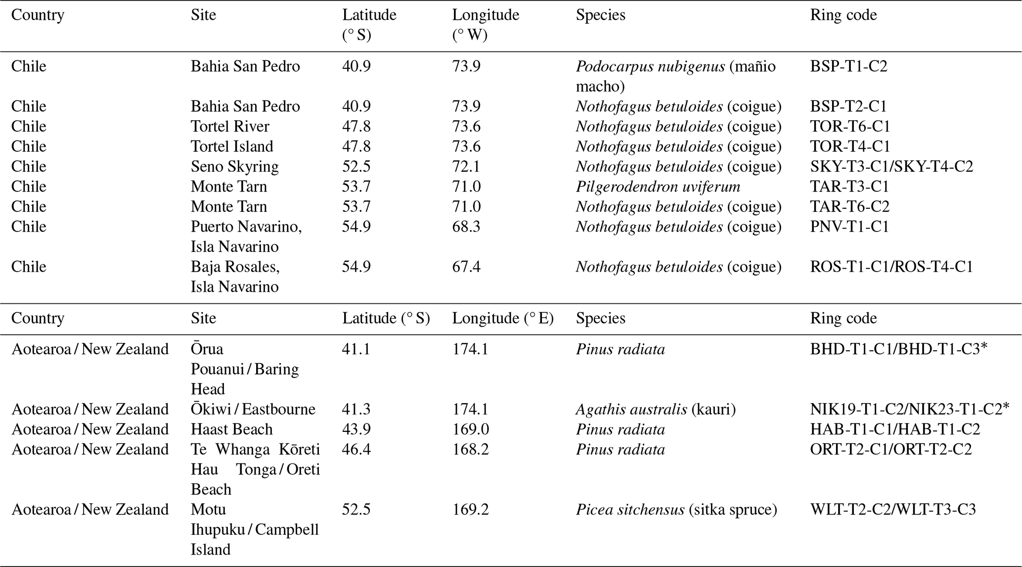
Tree-ring sampling in Aotearoa / New Zealand and Chile was conducted during field campaigns in 2016 and 2017. The west coasts of Chile, Aotearoa / New Zealand, and Aotearoa / New Zealand's subantarctic islands were selected because of the predominant westerly airflow which has oceanic influence and minimal terrestrial biospheric or anthropogenic influence (Fig. 2a and b, Table 1).

Table 1 Tabulation of site names, latitude and longitudes, species, and ring codes of trees that were selected and of cores that were used in the final work. The asterisk indicates that tree cores from Ōrua Pouanui / Baring Head and Ōkiwi / Eastbourne sites were previously published in Turnbull et al. (2017).

Traditional dendrochronology requires multiple trees within a stand of forest for reliable chronologies from annual growth rings. In this work, trees within stands were deliberately avoided in exchange for isolated specimens, often a few meters from the coast or on cliff tops directly sampling ocean air, to avoid the potential for reassimilation of respired CO₂ within the canopy. Trees were selected based on location close to the coast with minimal local land influences, feasibility of sampling (clear access to trunks and stable ground), clear and consistent rings, and consistency of species across multiple sites.

In short, cores were taken using a 4.3 mm increment corer (Haglöf Sweden), removed from the corer, and stored in straws to avoid damage during moving or storage. Tree cores were brought back to the Rafter Radiocarbon Laboratory (RRL) for sample workup and measurement. Cores were mounted onto aluminum-foil-coated cardboard with rubber bands, avoiding the glue traditionally used in dendrochronology. Only cores with clearly defined rings and unambiguous ring counts were considered for further analysis. These cores were sliced into single rings. All cores were sliced by a single person to ensure that any human bias in determining ring boundaries is consistent across all cores sampled in this study.

Sampled rings were then sliced longitudinally into thin “matchsticks” using a scalpel blade. They were then solvent-washed prior to cellulose extraction using hot acidified NaClO₂, followed by sodium hydroxide washes under a nitrogen atmosphere and a final acid wash (Norris, 2015; Corran, 2021). It has been demonstrated that this technique is sufficient to remove non-cellulosic material, whereas less rigorous techniques are not (Hua et al., 1999; Norris, 2015). Samples were combusted by elemental analyzer or sealed tube combustion (Baisden and Canessa, 2013), IRMS δ¹³C measurements were made on a subsampled aliquot of the resultant CO₂ gas, and the remaining CO₂ was graphitized (Turnbull et al., 2015) prior to ¹⁴C measurements made on our XCAMS system (Zondervan et al., 2015). Standardization is via Ox-I (Stuiver and Polach, 1977).

Results are reported as Δ¹⁴C (Stuiver and Polach 1977), corrected for decay according to the estimated middle date of each ring growth period. In the Southern Hemisphere, where the growth period spans 2 calendar years, dendrochronologists assign the ring year as the year that growth started, but the average age of the ring is estimated as 1 January of the following year for the purposes of radiocarbon decay correction. Uncertainties are determined from XCAMS counting statistics and the repeatability of replicate measurements of the tree-ring samples. The typical uncertainty is 2 ‰.

Ring counts must be validated to ensure proper chronologies and accurate interpretation of results; this is particularly important since the expected latitudinal gradients are of similar magnitude to the annual Δ¹⁴CO₂ trend. We primarily validated ring counts by Δ¹⁴C bomb spike matching: the rapid changes in Δ¹⁴C during the bomb spike are so much larger than the spatial variability, making a ring count error of a single year immediately apparent (Andreu-Hayles et al., 2015). Miscounted rings were easily identified by comparing measured Δ¹⁴C to the Ōrua Pouanui / Baring Head record (examples found in the Supplement). When a ring miscount was identified by this method, we discarded that core from further analysis. When we were unable to obtain tree cores from a given site that were long enough to include the bomb spike, ring counts were validated through duplicate sampling and cross-referencing of Δ¹⁴C measurements. Further information regarding ring count validation can be found in the Supplement. Cores from two sites (Ōrua Pouanui / Baring Head and Ōkiwi / Eastbourne) used in this work have been previously published (Turnbull et al., 2017).

2.2 Development of background reference

To put the tree-ring measurements into context, they are analyzed relative to Southern Hemisphere atmospheric background Δ¹⁴CO₂ from long-term measurements at Ōrua Pouanui / Baring Head, Aotearoa / New Zealand (GNS/NIWA) (Turnbull et al., 2017), and Kennaook / Cape Grim, Lutruwita / Tasmania (University of Heidelberg) (Levin et al., 2010), each described below. While modeling studies show lower Δ¹⁴C values over the Southern Ocean attributed to the upwelling of old, ¹⁴C-depleted waters (Graven et al., 2012; Levin et al., 2010), the Ōrua Pouanui / Baring Head and Kennaook / Cape Grim records from 41° S are not significantly influenced by the Southern Ocean signal (Levin et al., 2010), making them an appropriate anchor point. They are also the most complete and detailed in the Southern Hemisphere, making them a reliable reference.

The Ōrua Pouanui / Baring Head/Te Whanganui-a-Tara / Wellington record is the longest-running Δ¹⁴CO₂ dataset in the world and the only direct Southern Hemisphere atmospheric record to capture the ¹⁴C “bomb spike”. Beginning in 1954, this record has seen changes in methods and sampling sites over the years, discussed in detail in Turnbull et al. (2017). There is additional noise in the record starting from 1995, when RRL switched methods of Δ¹⁴C measurement from gas counting to AMS. In 2005, online ¹³C measurement allowed for appropriate fractionation correction and reduction in this noise (Turnbull et al., 2017; Zondervan et al., 2015). Data in the period between 2009 and 2012 are also significantly offset from the time series, which is thought to be due to changes in NaOH absorption sampling techniques during this period. These two periods (1995–2005 and 2009–2012) are therefore removed from the Te Whanganui-a-Tara / Wellington Record (Fig. 1b).

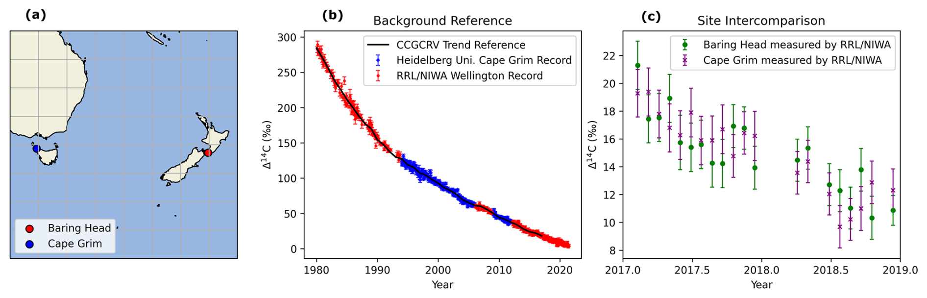
Figure 1 (a) Locations of Southern Hemisphere atmospheric background records – Kennaook / Cape Grim, Lutruwita / Tasmania, and Ōrua Pouanui / Baring Head, Te Whanganui-a-Tara / Wellington, Aotearoa / New Zealand. (b) Atmospheric Δ¹⁴CO₂ measured at Ōrua Pouanui / Baring Head and Kennaook / Cape Grim post-1980. Certain periods of data have been removed; see Methods. (c) Comparison of Δ¹⁴CO₂ measured at the two sites by the same laboratory to identify potential spatially driven offsets in atmospheric background. None were found.

The University of Heidelberg Institute of Environmental Physics operates a network of time series stations measuring Δ¹⁴CO₂ samples using the NaOH absorption method (Levin et al., 2010) and analyzed via decay counting (Kromer and Munnich, 1992). The Kennaook / Cape Grim, Lutruwita / Tasmania, station (CGO; 40.68° S, 144.68° E; Levin et al., 2010, 2022; Levin and Hammer, 2022) is at a similar latitude to Te Whanganui-a-Tara / Wellington and has data available between 1987 and 2018, overlapping the Ōrua Pouanui / Baring Head record from 1987–2016 (Fig. 1a and b).

The two time series from Ōrua Pouanui / Baring Head and Kennaook / Cape Grim are combined to fill gaps that exist in both records. Two issues that arise are (1) site–site offsets and (2) Δ¹⁴C measurement offsets. Justifications for the merging of two datasets from different sites are (1) Kennaook / Cape Grim and Te Whanganui-a-Tara / Wellington observe air masses of similar origin (Ziehn et al., 2014), and (2) a 2-year site–site intercomparison in which air samples collected from Ōrua Pouanui / Baring Head and Kennaook / Cape Grim were both processed and measured at NIWA/GNS found no measurable difference between the sites (Fig. 1c). Comparability between Δ¹⁴C measurements at RRL and those from the University of Heidelberg is within goals re-established by the WMO and GGMT in 2020 (0.5 ‰) (Crotwell et al., 2020). The merged dataset will subsequently be referred to as the “Southern Hemisphere Background” or the SHB.

2.3 Interfacing samples with reference datasets

The merged SHB contains discrete temporal values (sampling dates/times), representing the date a whole-air flask sample was collected or the median sampling date for passive NaOH absorption. The tree-ring Δ¹⁴CO₂ data have time values set to 1 January (summer) of the growth year. In order to estimate the difference between the tree-ring Δ¹⁴CO₂ and the SHB, the time axis of both datasets must be matched.

We use the NOAA Global Monitoring Laboratory's CCGCRV curve-fitting method (Thoning et al., 1989) to interpolate and smooth the SHB for comparison with the tree-ring Δ¹⁴CO₂, using a fast Fourier transform filter cutoff of 667 d. The goal is to reduce the noise associated with the relatively large uncertainties on individual Δ¹⁴C measurements, which can result in a single outlier Δ¹⁴C measurement in the SHB record aliasing into a deviation in ΔΔ¹⁴C in all the other records. Uncertainties on the smoothed, interpolated data are obtained using a Monte Carlo scheme run to 10 000 iterations as in Turnbull et al. (2017) and Hua et al. (2021). More information about this scheme can be found in the Supplement. The mean of the SHB smoothed data for October to March is used for comparison with the tree-ring Δ¹⁴CO₂. Taking the difference between tree-ring Δ¹⁴CO₂ and the “trended” SHB yields ΔΔ¹⁴CO₂ (Eq. 1).

$$\begin{array}{}\text{(1)}& \mathrm{\Delta }{\mathrm{\Delta }}^{\mathrm{14}}{\mathrm{CO}}_{\mathrm{2}}={\mathrm{\Delta }}^{\mathrm{14}}{\mathrm{CO}}_{\mathrm{2}\mathrm{\_}\mathrm{TreeRing}}-{\mathrm{\Delta }}^{\mathrm{14}}{\mathrm{CO}}_{\mathrm{2}\mathrm{\_}\mathrm{SHB}}\end{array}$$

2.4 Sampled time period

While the tree-ring records in some cases extend back to < 1950 and we measured some tree rings from the initial bomb spike to validate the ring counts, this study focuses on the “post-bomb period” from 1980 to 2017 (Turnbull et al., 2016). After the thermonuclear weapons testing created the radiocarbon “bomb spike”, isofluxes (differences between reservoir and atmosphere) from the terrestrial biosphere and the ocean to the atmosphere were strongly negative, as the systems were in severe disequilibrium (Levin et al., 2010; Naegler and Levin, 2009; Randerson et al., 2002; Turnbull et al., 2016). We select our samples post-1980 when equilibrium was closer to being established, the sign in biosphere isoflux had changed to positive, and the fossil fuel and ocean signals became the dominant drivers of Δ¹⁴C spatial variability (Levin et al., 2010; Naegler and Levin, 2009; Randerson et al., 2002; Turnbull et al., 2016). Biosphere respiration of bomb ¹⁴C now has higher Δ¹⁴C than the atmosphere, while the oceans still have a Δ¹⁴C lower than the atmosphere, with the possible exception of some tropical regions (Graven et al., 2012). Fossil fuels always have strongly negative isofluxes, essentially diluting atmospheric ¹⁴C (Suess 1955; Turnbull et al., 2016); however, in this Southern Hemisphere study, we aim to avoid local fossil fuel contribution.

2.5 Atmospheric back trajectories

We use the NOAA HYSPLIT air parcel trajectory model to estimate the source regions of air parcels arriving at each sampling site. We determined mean back trajectories by running HYSPLIT in the backwards mode with starting trajectories once every 2 d for the 3 months through the height of the growing season, running backwards in time for 6 d (December, January, February) for selected years during which meteorological data were available. The years 2005–2006, 2010–2011, 2015–2016, and 2020–2021 were selected. For each site, 185 trajectories were produced. This number of trajectories was selected to give a reasonable representation of the air-mass origins over the full time period, while balancing the computational effort required. Results are presented as a heat map showing the distribution of points over the trajectories. HYSPLIT was run via the Python PySPLIT package (Warner, 2018).

Air-mass back-trajectory results are analyzed in context to previously constrained Southern Ocean fronts and zones. We use the subtropical front (STF), subantarctic front (SAF), polar front (PF), and southern boundary (SB) from Orsi et al. (1995) as well as the climatological PF from Freeman and Lovenduski (2016). Climatological fronts from these works were chosen because of their data availability and overlap with the time span of our tree-ring measurements (1980–2017). Orsi et al. (1995) constrain the STF, SAF, PF, and SB using all available data up to 1990, while Freeman and Lovenduski (2016) PF climatology uses data from 2002 to 2014. Southern Ocean zones are defined as the region between the fronts, similar to Gray et al. (2018): the subtropical zone (STZ), subantarctic zone (SAZ), polar frontal zone (PFZ), Antarctic Southern Zone (ASZ), and Seasonal Ice Zone (SIZ) (see Fig. 4). Because our analysis overlaps with the time spans of Orsi et al. (1995) and Freeman and Lovenduski (2016) climatologies, we analyzed HYSPLIT back-trajectory results and GLODAP data (see Sect. 2.5) using both PF positions and reported the mean. Changes to the PF position, in our analysis, affect only the PFZ and ASZ results as the remaining fronts are held constant from Orsi et al. (1995).

2.6 GLODAP Ocean ¹⁴C data

The GLODAP Merged and Adjusted Data Product v2.2023 is used to add context to the discussion of our results (Key et al., 2004; Lauvset et al., 2023; Olsen et al., 2016). The data were filtered for existing radiocarbon measurements of ocean-dissolved inorganic carbon (“G2c14”) south of 5° S, shallower than 100 m, and post-1980 to match our tree-ring temporal span. Frontal zones from Orsi et al. (1995) were interpolated to distinct longitude values of samples in the dataset, to allow comparison of the sample latitude to front latitudes. Then, each measurement was “binned” in one of the Southern Ocean frontal zones (and ocean sectors), based on sample latitudes/longitudes. Further details on interpolation are included in the Supplement. The Pacific Sector is defined as between 120° E and 70° W, and the Indian Sector is between 21 and 120° E. The mean and standard deviations for nitrate and Δ¹⁴C, by ocean sector (and total ocean), for each polar frontal zone are shown in Fig. 6c and d and tabulated in the Supplement.

3 Results and discussion

The Δ¹⁴CO₂ measurements from each site are overlaid with the SHB (Fig. 2c and d) to show an overview of the data. All records reflect the general long-term pattern of decreasing Δ¹⁴CO₂ that is observed in the SHB record and globally. Small deviations from the SHB record become apparent when ΔΔ¹⁴CO₂ is calculated for each site (Fig. 2e and f). The inset histogram shows the distribution of all data from the Aotearoa / New Zealand or Chilean Sector. The most prominent feature of Fig. 2e and f is the year-to-year variability at all locations, likely driven by a combination of interannual variability in oceanic ¹⁴C fluxes, atmospheric transport, and tree growth periods. This paper intends to evaluate latitudinal gradients only. Temporal trends will be discussed further in a forthcoming paper. Raw Δ¹⁴CO₂ data (Fig. 2e and f) are not temporally de-trended before means are taken (data in Fig. 3).

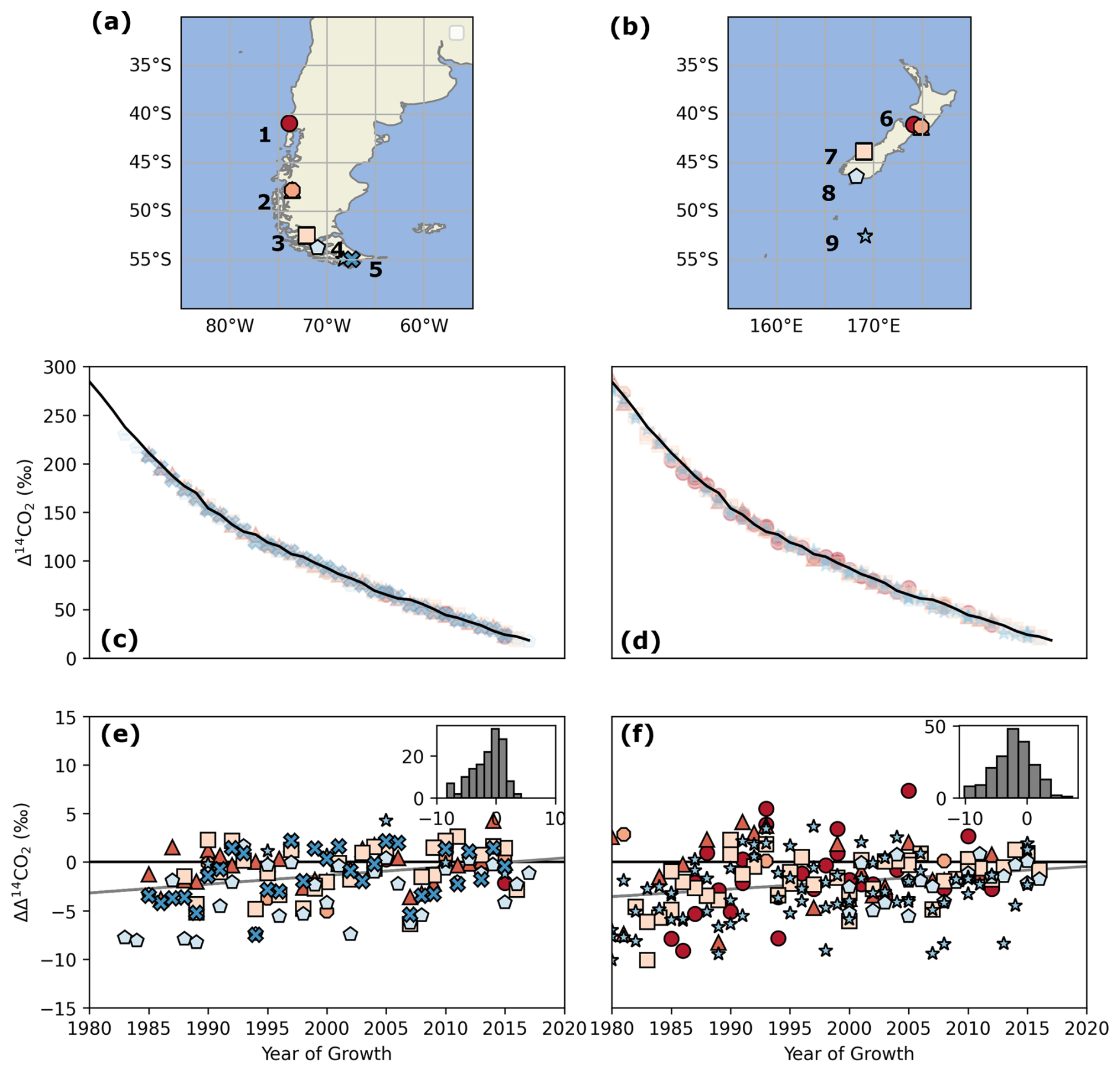
Figure 2 Panels (a) and (b) show the sampling sites in Chile and Aotearoa / New Zealand. The numbers refer to stations as follows: (1) Bahia San Pedro, (2) Tortel River and Tortel Island, (3) Seno Skyring, (4) Monte Tarn, Punta Arenas, (5) Puerto Navarino and Baja Rosales, Isla Navarino, (6) Ōrua Pouanui / Baring Head and Ōkiwi / Eastbourne, (7) Haast Beach, (8) Te Whanga Kōreti Hau Tonga / Oreti Beach, and (9) Motu Ihupuku / Campbell Island. Panels (c) and (d) show the measured Δ¹⁴CO₂ values overlaid onto the Southern Hemisphere background and smoothed with the CCGCRV algorithm. Panels (e) and (f) show the difference between the tree-ring Δ¹⁴CO₂ and the Southern Hemisphere Background (ΔΔ¹⁴CO₂). Inset histograms reflect all data from respective continents binned into 10 equal bins.

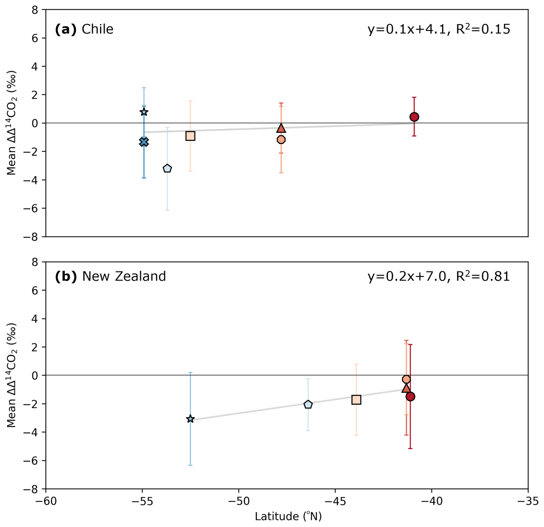
Figure 3 Mean ΔΔ¹⁴CO₂ values for each individual site in (a) Chile and (b) Aotearoa / New Zealand. Symbols and colors correspond to Fig. 2. Error bars represent the 1 standard deviation of the mean of each site's dataset of ΔΔ¹⁴CO₂ measurements, with each individual measurement error propagated throughout the analysis. A version of this figure with individual ΔΔ¹⁴CO₂ values and 95 % confidence intervals overlaid can be found in the Supplement.

3.1 Comparison with other Southern Hemisphere atmospheric Δ¹⁴C records

The measurements presented here expand the Southern Hemisphere records of atmospheric Δ¹⁴C previously described in Levin et al. (2010) and Hua et al. (2021). We briefly compare these new data to existing Southern Hemisphere Δ¹⁴C datasets at Kennaook / Cape Grim (Australia) (Levin et al., 2010), Motu Ihupuku / Campbell Island (Manning et al., 1990; Turney et al., 2018), Macquarie Island (Levin et al., 2010), and Neumayer Station (Levin et al., 2010).

In Turnbull et al. (2017), the authors publish Ōrua Pouanui / Baring Head and Ōkiwi / Eastbourne tree-ring Δ¹⁴C measurements and provide a rigorous comparison to show that the Te Whanganui-a-Tara / Wellington Δ¹⁴CO₂ record agrees well with atmospheric measurements from Kennaook / Cape Grim, Australia (Levin et al., 2010, 2022). An additional 2-year site–site intercomparison provides confidence that Kennaook / Cape Grim and Ōrua Pouanui / Baring Head are not different (Fig. 1c).

Manning et al. (1990) and Turney et al. (2018) report atmospheric and tree-ring measurements from Motu Ihupuku / Campbell Island, respectively. The atmospheric record from Manning et al. (1990) extends from 1970–1977 and does not overlap with our tree-ring measurements, ruling out a direct comparison with our Motu Ihupuku / Campbell Island tree rings. Turney et al. (2018) include tree-ring measurements from the same Sitka spruce tree, but the record only extends to 1967, disallowing a direct comparison. The Dracophyllum records extend from 1952 to 2011, overlapping well with our record. When the Turney et al. (2018) Dracophyllum records are analyzed according to our workflow, we find there is a robust difference (p < 0.05) between them and the Motu Ihupuku / Campbell Island record presented in this work (see Supplement), with Turney et al. (2018) offset higher. Fossil fuel CO₂ would drive Δ¹⁴CO₂ lower, but this is highly unlikely due to the absence of fossil influence in the region (Levin et al., 2010) and the uninhabited nature of the island. Biospheric contamination leading to a relative increase in the Turney et al. (2018) data is similarly unlikely due to sustained high westerly winds. We think the most likely explanation is an interlaboratory offset. However, an important consideration is that the records and results we show were all sampled, processed, and measured identically, meaning results from Motu Ihupuku / Campbell Island are best viewed relative to other sites from this work. Additionally, low values at Motu Ihupuku / Campbell Island can be validated by matching the Macquarie Island record (see below), where interlaboratory offsets between the two institutions have been investigated and none found (see Ōrua Pouanui / Baring Head versus Kennaook / Cape Grim, above, and Hammer et al., 2017).

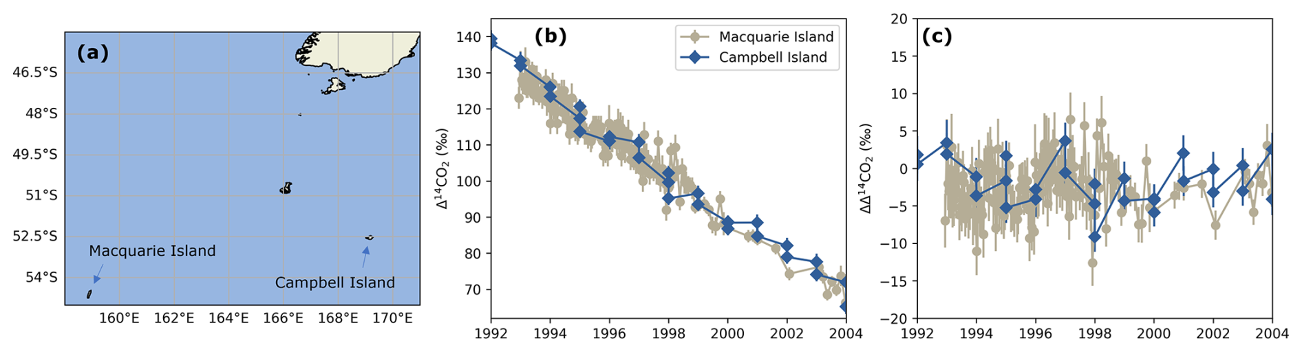
Figure 4 (a) Proximity of Macquarie Island (Levin et al., 2010) and Motu Ihupuku / Campbell Island. (b) The Δ¹⁴CO₂ values and (c) the ΔΔ¹⁴CO₂ values from Motu Ihupuku / Campbell Island and Macquarie Island.

It is instructive to compare Motu Ihupuku / Campbell Island (52.5° S, 169.2° E) to the nearby Macquarie Island atmospheric record (54.6° S, 158.9° E) from 1992 to 2004 (Levin et al., 2010). Figure 4 shows direct comparisons of the sites' Δ¹⁴CO₂ and ΔΔ¹⁴CO₂. The latter shows when the Macquarie Island record is analyzed in our workflow. The Macquarie Island atmospheric record is −2.6 ± 3.2 ‰ lower than the background, similar to Motu Ihupuku / Campbell Island ΔΔ¹⁴C. The independent t test also shows the datasets are not different (p = 0.3). This specific comparison provides confidence that the result we find at Motu Ihupuku / Campbell Island is robust. Macquarie Island is previously the only record at this latitudinal band to capture low Δ¹⁴C over the Southern Ocean. The new Motu Ihupuku / Campbell Island record not only supports the original Macquarie Island record but also extends back to 1980 and forward to 2017.

Levin et al. (2010) found that Macquarie Island and Neumayer Station atmospheric records (70.4° S, 8.2° E) are both influenced by Southern Ocean outgassing. Comparing Neumayer Station and Motu Ihupuku / Campbell Island shows there is no robust difference between the sites (p = 0.5).

3.2 Aotearoa / New Zealand tree-ring Δ¹⁴C

The mean and 1 standard deviation of ΔΔ¹⁴CO₂ for each site over the record are shown in Fig. 3. The colors and symbols correspond to Fig. 2. The three sites at or near Ōrua Pouanui / Baring Head (the origin of the background record) (Fig. 3b) are close, but not identical, to the SHB. Tree rings incorporate air over a months-long growing season regardless of wind direction, while individual measurements used for the SHB are either a temporal snapshot (air flask sample) or a 2-week integration (NaOH absorption). This difference is a likely driver of such variability.

All Aotearoa / New Zealand sites' ΔΔ¹⁴CO₂ means are within 1σ of 0 ‰ besides Te Whanga Kōreti Hau Tonga / Oreti Beach (46° S). Nonetheless, there is a linear trend (R² = 0.81; p = ≪ 0.05) and steeper slope compared to that of Chilean sites. This slope is driven by our southernmost Aotearoa / New Zealand site, Motu Ihupuku / Campbell Island, with the lowest mean ΔΔ¹⁴CO₂ (−3.1 ± 3.3 ‰). Because our results are not temporally de-trended before the mean is taken, if Motu Ihupuku / Campbell Island tree rings indeed capture decadal variability in atmospheric Δ¹⁴C forced by changes in Southern Ocean outgassing, then this will increase the variability in the record. This will be further explored in future work.

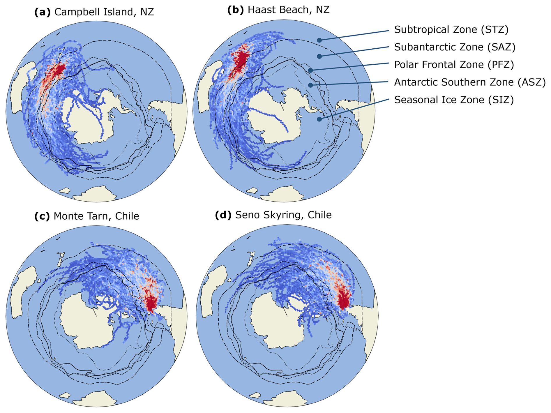
Figure 5 HYSPLIT back trajectories shown for select sites. Trajectories for all other sites are found in the Supplement. Southern Ocean fronts presented in bold are from Orsi et al. (1995) climatology and polar fronts presented as semitransparent regions are from Freeman and Lovenduski et al. (2016) climatology.

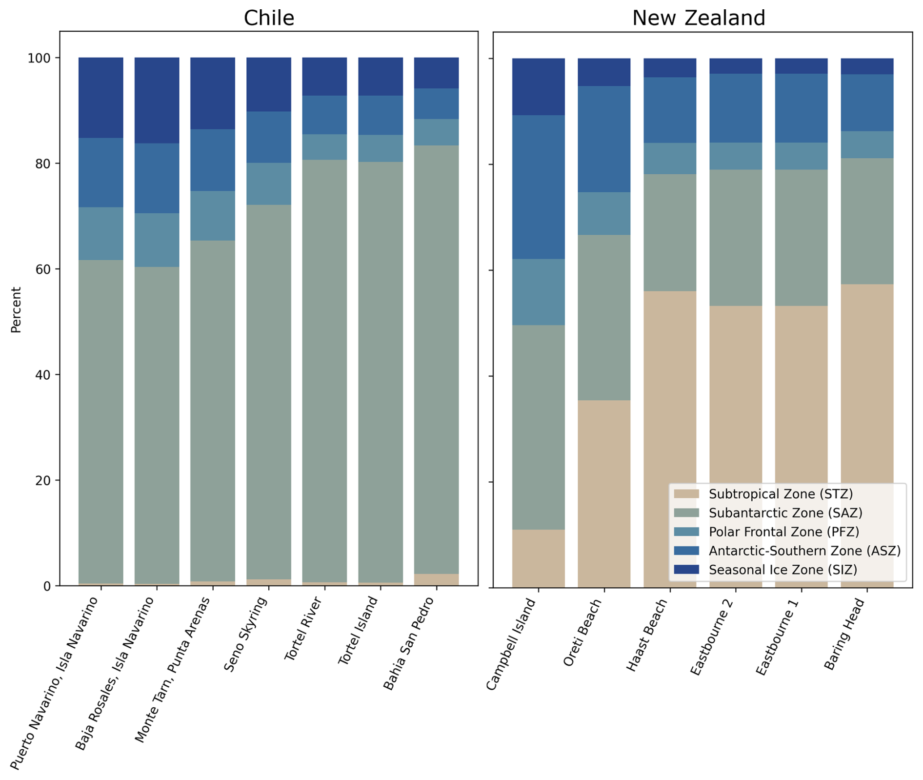
Figure 6 Visual representation of the amount of time HYSPLIT back trajectories from each site spend in each Southern Ocean frontal zone. PFZ and ASZ represent the mean of values calculated using PF climatology from Orsi et al. (1995) and Freeman and Lovenduski (2016).

Results from HYSPLIT back trajectories are displayed as heat maps for selected sites in Fig. 5, with remaining sites shown in the Supplement. Heat map data are also displayed as a bar chart in Fig. 6, with a table in the Supplement. Motu Ihupuku / Campbell Island is the only Aotearoa / New Zealand site where the HYSPLIT back-trajectory plume core sits in the SAZ. HYSPLIT modeling indicates that air moving toward Motu Ihupuku / Campbell Island spent the most amount of time in both the PFZ and ASZ (15.3 % and 24.4 %; Fig. 5). Most Southern Ocean outgassing occurs in these two zones, with the latter showing near-year-round outgassing (Gray et al., 2018).

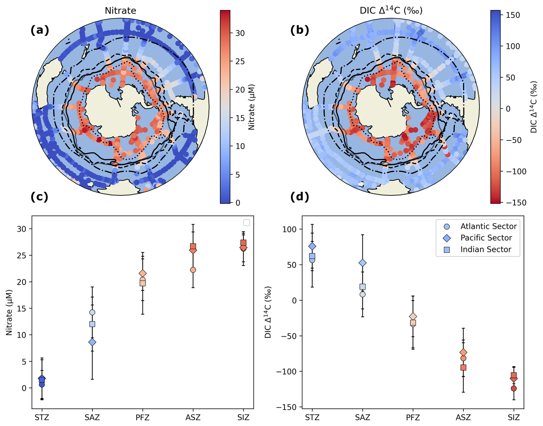
Figure 7 (a, b) Nitrate and DIC Δ¹⁴C data from the GLODAP Merged and Adjusted Data Product v2.2023 (Key et al., 2004; Lauvset et al., 2023; Olsen et al., 2016). Data were filtered for measurements south of 5° S and depths 0–100 m after 1980. (c, d) The mean and 1σ standard deviation of nitrate DIC Δ¹⁴C for each zone. Southern Ocean fronts presented in bold are from Orsi et al. (1995) and polar fronts presented as semitransparent regions are from Freeman and Lovenduski et al. (2016) climatology. In panels (c) and (d), PFZ and ASZ represent the mean of values calculated using PF climatology from Orsi et al. (1995) and Freeman and Lovenduski (2016).

Figure 7 shows nitrate and DIC Δ¹⁴C from GLODAP (see Methods). Nitrate increases and DIC Δ¹⁴C values decrease toward higher latitudes into the PFZ, ASZ, and SIZ. DIC Δ¹⁴C decreases by ∼ 150 ‰ between the STZ and ASZ. These are distinct markers not only of Southern Ocean upwelling but also of low Δ¹⁴C values imparted from old surface water masses to overlying air masses carried on to our tree-ring sites. We hypothesize that the Aotearoa / New Zealand ΔΔ¹⁴CO₂ latitudinal gradient is driven by Southern Ocean outgassing in the PFZ and ASZ which feed air to Motu Ihupuku / Campbell Island in greater abundance relative to more northern sites. Motu Ihupuku / Campbell Island tree rings may therefore be useful for detecting changes in outgassing in the Indian Ocean Sector of the Southern Ocean PFZ and ASZ.

3.3 Chilean tree-ring Δ¹⁴C

A weak latitudinal gradient exists in the Chile dataset; however, this is driven by one site (Monte Tarn; 53.7° S). Excluding this site, all means are indistinguishable from the SHB, and the linear regression slope falls from 0.1 to 0.03 and R² from 0.15 to 0.05 (p = 0.4). Including all data, the Chilean trend has a p value of 0.395 and is not statistically significant.

Monte Tarn has the lowest mean ΔΔ¹⁴CO₂, is the only site outside 1σ of the SHB (mean = −3.2 ± 2.9 ‰), and, notably, is not the most southerly Chilean site. It is also shrouded by the mountainous barrier island, Isla Clarence, and is near a shipping lane leading to Punta Arenas. Sites in this study were specifically chosen on western coastlines to maximize the amount of clean ocean air originating from predominant westerlies around the ACC. This makes the likelihood of fossil fuel CO₂ incorporation into the tree rings low. Fossil CO₂ incorporation would lower ΔΔ¹⁴C in Monte Tarn tree rings; however, it is difficult to compose an estimate of the magnitude due to the privacy of shipping data.

Our southernmost Chilean records are two sites on Isla Navarino at the same latitude of 54.9° S. Of the two, Puerto Navarino lies further west and is in proximity to the Argentinian city of Ushuaia, while Baja Rosales is 0.9° to the east. These two sites were selected with the expectation that any significant land biosphere signal or fossil fuel emissions from urban influence would lead to measurable differences between the two sites. However, no statistically significant offset is found between them (see the Supplement). Mean ΔΔ¹⁴CO₂ values of both sites are within 1σ of zero (Puerto Navarino: 0.8 ± 1.7 ‰; Baja Rosales: −1.3 ± 2.5 ‰).

3.4 Ocean sector influence on atmospheric Δ¹⁴CO₂

We hypothesize that steeper latitudinal gradients are found in Aotearoa / New Zealand versus Chilean sites due to variability in the spatial extent of Southern Ocean zones in the Indian Ocean and the Pacific Ocean and to differences in Δ¹⁴C values of DIC upwelling in the ASZ in the Indian Sector versus Pacific Sector.

Southern Ocean carbon flux is complex and variable, with different sectors acting as sources and sinks for anthropogenic and natural CO₂, respectively (Gruber et al., 2019). The Southern Ocean as a whole acts as a sink for anthropogenic CO₂, with uptake concentrated in the PFZ (Mikaloff Fletcher et al. 2006, DeVries 2014; Gruber et al., 2019). In the case of natural CO₂, higher latitudes, specifically those of the ASZ and PFZ, dominate outgassing, while lower latitudes such as in the STZ dominate uptake (Gruber et al., 2019). Some zones outgas seasonally, while the ASZ outgasses nearly year-round (Gray et al., 2018). Uptake and outgassing are also zonally asymmetric. The Indian Sector and Pacific Sector jointly dominate Southern Ocean outgassing. These complexities play key roles in facilitating a signal of one-way flux of low Δ¹⁴C from the surface ocean toward distant trees.

Hypothetically, if the amounts of CO₂ originating from the same proportion of high-latitude Southern Ocean zones (SIZ, ASZ, and PFZ) reaching Chile and Aotearoa / New Zealand were equal, it would be reasonable to assume that our method should find the same gradient in ΔΔ¹⁴CO₂ with latitude for Chilean and Aotearoa / New Zealand tree rings. The Pacific has higher DIC and lower O₂ concentrations in Indian–Pacific Deep Waters, which upwell around the ACC band (Chen et al., 2022), suggesting it is more carbon rich and old. The Pacific also dominates outgassing in the PFZ (Prend et al., 2022). With these conditions, one would expect lower ΔΔ¹⁴CO₂ values in Chilean tree rings than Aotearoa / New Zealand tree rings.

Despite this, we find a stronger outgassing influence in Aotearoa / New Zealand, which lies east of the Indian Ocean. This discrepancy is especially prominent if the Chilean site Monte Tarn is excluded due to its proximity to a shipping lane, leaving Motu Ihupuku / Campbell Island with the lowest ΔΔ¹⁴CO₂ value.

We hypothesize that the driving factor is the fact that a larger proportion of Aotearoa / New Zealand back trajectories lie in the crucial year-round outgassing ASZ because the zone is expanded in the Indian Ocean Sector relative to the Pacific Ocean Sector. The ASZ surface also has lower Δ¹⁴C than more northerly zones (Fig. 6d), amplifying the effect of atmospheric dilution of ¹⁴C relative to outgassing in general. Due to Motu Ihupuku / Campbell Island trees' ability to capture dilution in atmospheric Δ¹⁴C from Southern Ocean outgassing, tree rings from this site may be a viable candidate to reconstruct changes in Southern Ocean outgassing from the past few decades.

4 Conclusion

While other methods of estimating Southern Ocean air–sea CO₂ flux face the challenge of distinguishing between two large opposing forces (outgassing of natural CO₂ and uptake of natural CO₂), radiocarbon measurements through long-term atmospheric records (Levin et al., 2010) or tree rings allow us to constrain a one-way flux by measuring dilution of atmospheric radiocarbon from outgassing of CO₂ from aged water masses. They also provide the opportunity to reconstruct changes in the past when hydrographic and float-based data were sparse. We report a novel database of 280 unique tree-ring Δ¹⁴C measurements from Chile and Aotearoa / New Zealand from 1980–2017. This work substantially expands the Δ¹⁴C records from the southern mid-high latitudes and is consistent with previous studies that demonstrate the imprint of Southern Ocean upwelling on atmospheric Δ¹⁴C in the Southern Hemisphere (Levin et al., 2010; Graven et al., 2012). The upwelling signal is most apparent at Motu Ihupuku / Campbell Island, the southernmost Aotearoa / New Zealand site that has HYSPLIT back-trajectory footprints in the ASZ, which is the only ocean zone to exhibit year-round outgassing (Gray et al., 2018). The link between low ΔΔ¹⁴CO₂ in Motu Ihupuku / Campbell Island tree rings and air-mass origination in the Indian Sector of the ASZ should be further explored for viability as a proxy for detecting changes in upwelling.

Data at more northerly sites and those that are influenced by air masses from lower-latitude ocean zones appear fairly homogenous. This suggests that the influence of non-local fossil fuel and biospheric signals is small in the Southern Hemisphere. Further investigation is required to understand the mechanism behind low values at the Chilean site Monte Tarn and if fossil fuel contamination from a nearby shipping lane may play a role.

Tree-ring Δ¹⁴C measurements are key tools to reconstruct atmospheric Δ¹⁴C and may provide new opportunities when trying to understand changes in Southern Ocean upwelling and air–sea CO₂ flux. This work also highlights the potential for ship-based atmospheric Δ¹⁴C measurements to detect changes in ocean upwelling. Ship-based atmospheric Δ¹⁴C samples can be collected with higher temporal frequency, without the need for oceanographic research vessels. More investigation is required to understand temporal changes in ΔΔ¹⁴CO₂. In a companion work to follow, we will address trends over time and analyze how our trends compare with Le Quéré et al. (2007) and ocean model output.