Northern North Atlantic climate variability controls on ocean carbon sinks in EC-Earth3-CC

The northern North Atlantic (NA) is an important net sink of atmospheric CO₂, though atmosphere–ocean CO₂ fluxes exhibit substantial variability across different timescales. The underlying drivers of this variability remain poorly understood across both temporal and regional scales. Here, we investigate interannual to decadal CO₂ flux variability in the northern NA using historical simulations from the EC-Earth3-CC model. We assess the role of key dynamical and physical processes in shaping CO₂ flux variability across five regions: the Nordic Seas (NS), eastern NS, the eastern and western subpolar NA, and the full NA. Our analysis reveals that physical parameters – including sea ice concentration (SIC), sea surface temperature (SST), sea surface salinity (SSS), and wind stress – along with dynamical processes related to ocean mixing and circulation, play a central role in regulating CO₂ flux variability. Using regression analysis, we demonstrate that these drivers exert regionally and temporally varying influences, with our models achieving high R² values indicating a strong degree of explanation for CO₂ flux variability. The regression models capture interannual variability more effectively than decadal variability, highlighting the dominant role of short-term fluctuations in shaping CO₂ flux dynamics. Overall, our results demonstrate that the predictors of CO₂ flux variability are both spatially and temporally dependent. We find that CO₂ flux variability cannot be fully explained by simple linear correlations with individual predictors but instead arises from complex interactions among multiple physical and dynamical processes. Notably, CO₂ flux variability is particularly sensitive to changes in certain predictors, such as wind stress, consistent with expectations based on the gas transfer equation used to compute atmosphere–ocean CO₂ fluxes.

1 Introduction

The northern North Atlantic (NA) is a net sink of atmospheric carbon dioxide (CO₂; Fig. 1a; Gruber et al., 2002; Takahashi et al., 2009; Yu et al., 2019). This sink is primarily driven by the combined effects of the solubility pump and the biological carbon pump. The solubility pump enhances CO₂ uptake through two key mechanisms: (1) the cooling of northward-flowing warm waters, which increases CO₂ solubility at the surface, and (2) the formation of dense, cold deep water at high latitudes, which transports CO₂-enriched surface waters into the ocean interior as part of the Atlantic thermohaline circulation (Volk and Hoffert, 1985). The biological carbon pump further contributes by fixating carbon through photosynthesis and primary production (PP), exporting organic carbon to the deep ocean, and maintaining a net sink of atmospheric CO₂ in the region (Sigman and Boyle, 2000; Boyd and Trull, 2007; Sanders et al., 2014). Currently, the NA absorbs a significant fraction of anthropogenic CO₂ emissions, accounting for approximately one-quarter to one-third of global anthropogenic carbon uptake (Khatiwala et al., 2009; Sabine et al., 2004; Breeden and McKinley, 2016; Le Quéré et al., 2018; Gruber et al., 2019). In contrast, the global ocean uptake is approximately 25 % of annual emissions due to outgassing in some ocean regions (Fig. 1; Landschützer et al., 2016; Mikaloff Fletcher et al., 2006; Khatiwala et al., 2013; Le Quéré et al., 2015; Friedlingstein et al., 2025; Gruber et al., 2023; Terhaar et al., 2022).

Beyond these large-scale mechanisms, the strength of the NA CO₂ sink varies seasonally and interannually, influenced by ocean–atmosphere interactions. Biological productivity peaks in spring and summer, enhancing CO₂ drawdown, while wintertime cooling promotes solubility-driven uptake (Ardyna and Arrigo, 2020). These processes are modulated by climate variability, particularly the NA Oscillation (NAO) and the Atlantic Multidecadal Oscillation (AMO; Leseurre et al., 2020). In addition, physical processes such as warming and cooling cycles, deep convection, and changes in ocean circulation and water masses in the subpolar gyre (SPG) play a crucial role in regulating air–sea CO₂ fluxes. These physical drivers are closely linked to NAO and AMO variability, further influencing regional CO₂ uptake dynamics (Chafik and Rossby, 2019; Desbruyères et al., 2019). Breeden and McKinley (2016) show that a NA basin-average sea surface temperature (SST) is associated with the leading mode of surface ocean pCO₂ variability based on an analysis of a regional model. The SST signal is affected by an upward trend due to greenhouse gas emissions and a signal of internal variability due to the AMO (Kerr, 2000). Furthermore, they establish that physical (in contrast to chemical) variability is the dominant driver of variability in the NA surface ocean carbon cycle. During a positive phase of the AMO an increase in sea (surface) temperature increases pCO₂ due to the reduction in solubility (an increase in the fugacity of CO₂, fCO₂) resulting in a reduced flux of CO₂ into the ocean (also seen in Breeden and McKinley, 2016). Studies show that on a decadal scale the AMO and fCO₂ variability in the SPG correlates (Breeden and McKinley, 2016; Landschützer et al., 2016; Leseurre et al., 2020): as the AMO enters a positive (warm) phase, reduced mixing (a shallowing of the mixed layer depth (MLD)) results in a reduced supply of dissolved inorganic carbon (DIC) from the subsurface layers, a process that dominates the effect of warming on the solubility and fCO₂. The surface ocean's ability to absorb anthropogenic carbon is primarily regulated by carbonate chemistry, particularly alkalinity (Broecker et al., 1979; Terhaar et al., 2022). While increasing anthropogenic carbon generally enhances ocean carbon uptake, this relationship is moderated by rising global temperatures, which reduce solubility, and is further influenced by decadal variability and long-term trends. However, the underlying drivers of these trends remain poorly understood (Terhaar, 2024).

The subpolar NA has experienced significant interannual to decadal variability in ventilation depth during the industrial period (Polyakov et al., 2005; Holliday et al., 2020; Zou et al., 2023; Thomas and Zhang, 2022). Recent studies highlight pronounced ocean variability in the SPG region, including the formation of cold and fresh anomalies. Holliday et al. (2020) documented a substantial freshening event in the eastern subpolar NA, the most significant in 120 years, attributed to wind-driven circulation changes that redistributed freshwater within the region. Similarly, Zou et al. (2023) identified two sources of deep ocean variability in the central Labrador Sea, furthering our understanding of long-term property anomalies in the western subpolar NA. These findings underscore the SPG's dynamic nature and its sensitivity to both atmospheric and oceanic forcing. The SPG, a anticlockwise gyre system, plays a crucial role in modulating ocean circulation by introducing saline Atlantic water into the northern NA. The NA Current follows the southern and eastern boundaries of the SPG, transporting warm, saline water from the Gulf Stream into the northern NA and eventually the Arctic (Holliday et al., 2020; Daniault et al., 2016; Hátún et al., 2017). At the same time, freshwater from the Arctic is supplied to the SPG, contributing to temporal variability in ocean properties. These processes are key regulators of the Atlantic Meridional Ocean Circulation (AMOC) (Holliday et al., 2020; Hátún et al., 2005, 2017). The strength of the SPG circulation strongly influences both physical and biological processes in the northern NA. A weak (strong) SPG leads to a shallowing (deepening) of sea surface height (SSH) and, consequently, a shallowing (deepening) of the MLD. In addition, a weak SPG contracts westward, allowing nutrient-poor subtropical waters to penetrate northward, warming the gyre and reducing PP. In contrast, a strong SPG expands eastward, accumulates Arctic fresh and nutrient-rich water within the gyre system, increasing PP and solubility, and limits the intrusion of warm, saline Atlantic water into the region (Häkkinen et al., 2013; Hátún et al., 2005, 2017; Foukal and Lozier, 2017). Importantly, variations in sea surface salinity (SSS) serve as an indicator of these gyre dynamics and ocean mixing processes, making it a valuable indirect predictor of CO₂ flux variability. Changes in salinity reflect shifts in water mass distribution, stratification, and ventilation, all of which influence air–sea gas exchange. Therefore, monitoring SSS variability can provide critical insights into the mechanisms driving CO₂ flux variability in the North Atlantic (Thomas and Zhang, 2022).

Understanding the vulnerability of the ocean carbon sink to future climatic changes is the motivator for our analysis. Expected future decline in the strength of the AMOC (Fox-Kemper et al., 2021) will probably result in a declining ocean CO₂ uptake due to less transport of CO₂ enriched surface waters into the deep ocean. Projections indicate a reduced CO₂ uptake/sink in the global oceans correlating with a gradual reduction of the strength of the AMOC (McKinley et al., 2023; Liu et al., 2023). A slowing AMOC impacts ocean biology and solubility carbon pumps: CMIP5 analysis projects a weakening of the biological pump from surface waters with the largest decreases in effective CO₂ uptake under the strongest warming scenarios (Bopp et al., 2013; Fu et al., 2016; Laufkötter et al., 2016; Liu et al., 2023). This is in part explained by ocean warming, which results in a decline in PP, also contributing to a decrease in ocean CO₂ uptake in some regions (Kwiatkowski et al., 2020); however, ocean warming and climate change also leads to sea ice decline, which results in increased PP regionally (Vancoppenolle et al., 2013). The projected climate-driven impacts on the AMOC are yet not seen in the strength of regional components of the AMOC in the northern NA (Østerhus et al., 2019; Lozier et al., 2019; Orvik, 2022). Also, over the last two decades the estimated AMOC strength at 26° N is dominated by interannual to decadal variability with a marginal significant negative trend (Volkov et al., 2024). These findings underscore how variability in the NA ocean and climate conditions, including fluctuations in AMOC strength, can modulate both the magnitude and regional distribution of oceanic CO₂ sinks.

We aim to understand the sensitivity and drivers of the atmosphere–ocean CO₂ flux in an Earth system model on interannual and decadal timescales. Through our analysis we establish which predictors can explain the CO₂ flux variability in the five regions of the northern NA. We define regression models based on physical and dynamic predictors, to explore how well we can predict and understand future CO₂ flux variability.

1.1 Approach

The aim of this work is to understand how simulated interannual to decadal variability can help build confidence in future changes and a better understanding of uncertainties related to ocean processes and variability. We analyse ensemble data from 10 historical simulations with the EC-Earth3-CC global climate model with interactive ocean biogeochemical cycling. To assess the drivers of the interannual and decadal CO₂ flux variability in the northern NA we initially establish an overview of the relationship between the CO₂ flux variability and parameters that could potentially drive this variability across the northern NA and in defined subregions (Fig. 1b).

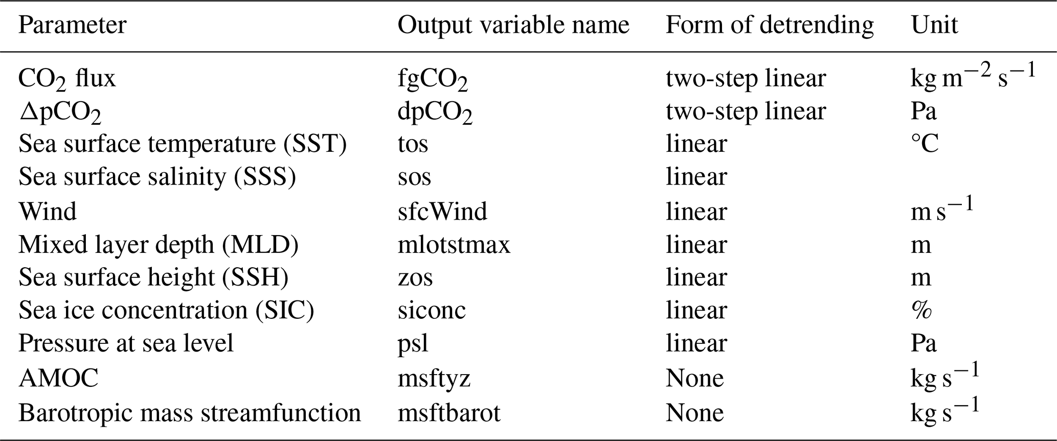
First, we use the gas transfer equations to check if we can reproduce the simulated CO₂ flux variability in the different regions from archived model data for the individual ocean region. Based on the gas transfer equation (Eqs. 1–3) we expect SST, SSS, ΔpCO_2, wind, and sea ice concentration (SIC) to be the controlling physical parameters driving the simulated CO₂ flux variability. We additionally explore the relation of the integral between CO₂ flux variability and parameters representing ocean dynamics or processes by including parameters such as MLD and sea surface height (SSH), which are not direct drivers of atmosphere–ocean gas exchange. For each region, we integrate the CO₂ flux and define high and low CO₂ flux years for short and long timescales. We construct ensemble mean composite two-dimensional maps of the CO₂ flux by subtracting the low flux years from the high flux years and by combining all ensemble members. We use the high and low flux years defined for the CO₂ flux to also construct composite maps of other key physical parameters.

Second, informed by the composite maps and identified controls of the CO₂ flux variability, we define 10 indexes that can be correlated with the CO₂ flux time series. The indexes are based on the parameters contributing to the gas exchange equations (Eqs. 1–3) SST (AMO), SSS, wind, and SIC, climatic modes of variability such as NAO, the ocean circulation strength (SSH index representing gyre circulation strength), MLD, and AMOC. The specific definition of the different indexes and why we have chosen them is described in Sect. 3. We have chosen to exclude ΔpCO₂ and other biogeochemical parameters, to focus our analysis on the physical processes and dynamical parameters affecting CO₂ flux variability.

Finally, in order to understand how much of the CO₂ flux variability that can be explained and described by physical variables and indexes alone, we set up simple linear multivariable regression models for each region and discuss differences in explained variability across interannual and decadal timescales.

1.2 EC-Earth3-CC

EC-Earth3-CC is the carbon cycle (CC) version of the EC-Earth3. EC-Earth3 is an Earth system model, developed by the EC-Earth consortium (https://ec-earth.org, last access: 10 March 2025), and contributes to the Coupled Model Intercomparison Project (CMIP). EC-Earth3 comprises several model components describing atmosphere, ocean, sea ice, land surface, dynamic vegetation, atmospheric chemical composition, ocean biogeochemistry, and the Greenland Ice Sheet. EC-Earth3 (Döscher et al., 2022) consists of the atmosphere model IFS, land surface module HTESSEL, and the ocean model NEMO3.6 (Madec and the NEMO team, 2015).

EC-Earth3-CC describes the CC and is used for the Coupled Climate-Carbon Cycle Model Intercomparison Project (C4MIP; Jones et al., 2016). The configuration allows for concentration-driven simulations and with emissions forcings. The CO₂ flux is calculated from and proportional to the difference in partial pressure of CO₂ (ΔpCO₂) between the atmosphere and the surface of the ocean (Döscher et al., 2022).

EC-Earth3-CC runs with NEMO3.6 coupled to PISCES-v2 (Pelagic Interactions Scheme for Carbon and Ecosystem Studies volume 2; Aumont et al., 2015), a biogeochemical model simulating marine biological productivity and the biogeochemical cycling of carbon and the main nutrients. Primary productivity is computed based on the availability of the main nutrients (P, N, Si, Fe), with a constant Redfield ratio ($\mathrm{P}:\mathrm{N}:\mathrm{C}=\mathrm{1}:\mathrm{16}:\mathrm{122}$) (Redfield ratio from Takahashi et al., 1985; Aumont et al., 2015). Air–sea gas exchange for carbon dioxide is parameterized from Wanninkhof (1992), updated in Wanninkhof (2014) to Eq. (1):

$$\begin{array}{}\text{(1)}& F=k{K}_{\mathrm{0}}({\mathrm{pCO}}_{\mathrm{2}\mathrm{w}}-{\mathrm{pCO}}_{\mathrm{2}\mathrm{a}}),\end{array}$$

where F is the flux (mass area⁻¹ time⁻¹), k is the gas transfer velocity (length time⁻¹), and K₀ is the solubility (mass volume⁻¹ pressure⁻¹), which is dependent on water temperature and salinity; pCO_2w and pCO_2a (pressure) are the partial pressures of CO₂ in equilibrium with surface water and the above lying air, respectively. The gas transfer velocity is dependent on wind speed according to Eq. (2):

$$\begin{array}{}\text{(2)}& k=\mathrm{0.251}{U}^{\mathrm{2}}{\left({\displaystyle \frac{\mathit{Sc}}{\mathrm{660}}}\right)}^{-\mathrm{0.5}},\end{array}$$

where U is the wind speed (10 m height) and Sc is the Schmidt number. The Schmidt number is dependent on water temperature. Furthermore, the CO₂ flux is dependent on SIC in the region, as no exchange is allowed between the atmosphere and sea water across sea ice Eq. (3):

$$\begin{array}{}\text{(3)}& {\mathrm{kgCO}}_{\mathrm{2}}=k{}^{\prime }{\mathrm{gCO}}_{\mathrm{2}}\times \left(\mathrm{1}{\mathit{\%}}_{\mathrm{ice}}\right),\end{array}$$

where kgCO₂ is the atmosphere–ocean CO₂ flux after correcting for SIC, k^′gCO₂ is the atmosphere–ocean CO₂ flux before correcting for SIC, %_ice is the concentration of sea ice, which varies between 0 and 1 (Döscher et al., 2022; Aumont et al., 2015).

The present-day (1982–2014) averaged air–sea CO₂ flux shows a general flux into the ocean in the NA and Nordic Seas (NS) (positive CO₂ flux, Fig. 1a–c). Observations show a similar pattern of a positive flux (CO₂ uptake in the ocean) in the NA and Arctic region, and a negative flux (outgassing to the atmosphere) off the western coast of Africa across the Atlantic and off the coast of South America (Fig. 1b). However, observations generally show a smaller air–sea CO₂ flux than simulated in EC-Earth3-CC (Fig. 1c). Döscher et al. (2022) shows that the EC-Earth3-CC air–sea CO₂ flux is in general overestimated in the high northern latitudes (>50° N) in the Northern Hemisphere, and underestimated in the high latitudes in the Southern Hemisphere. However, the general distribution of the air–sea CO₂ flux is well represented in EC-Earth3-CC (Fig. 1a–c).

The sea ice extent of EC-Earth3 (and therefore also EC-Earth3-CC) is in general overestimated in the NS and NA compared to observations (Döscher et al., 2022; Tian et al., 2021). As no exchange between the atmosphere and seawater is allowed across sea ice in EC-Earth3, an overestimation of the sea ice extent will inevitably affect the CO₂ flux. The global pattern of the CO₂ flux and the overestimation of the sea ice extent emphasizes the importance of sea ice and high latitude processes in the global climate system (Fig. 1).

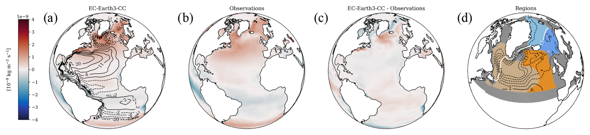
Figure 1 Atmosphere–ocean CO₂ flux averaged over the period 1982–2014 for (a) EC-Earth3-CC and (b) observation-based reconstruction CO₂ flux data from Gregor and Fay (2021), as well as (c) their difference. Black lines show the mean barotropic streamfunction of the SPG circulation of 10 ensemble members in Sv. Full lines indicate positive values, and dashed lines indicate negative values. Fully closed dashed lines indicate the shape and mean extent of the SPG in contrast to the open mean barotropic streamfunction contours. (d) Study regions: NA covering all regions (dark grey), SPW (beige), SPE (orange), NSE (blue), NS covering NSE as well (light blue), and global average 15 % SIC line (white contour) indicating the boundary between sea-ice-covered regions and sea-ice-free areas.

2 Data and methods

The analysis is based on EC-Earth3-CC historical runs 1850–2014 from all available ensemble members on ESGF (https://esgf-node.ipsl.upmc.fr/search/cmip6-ipsl/, last access: 15 September 2025) (10 ensemble members: r1i1p1f1, r4i1p1f1, r6i1p1f1, r7i1p1f1, r8i1p1f1, r9i1p1f1, r10i1p1f1, r11i1p1f1, r12i1p1f1, r13i1p1f1). We make use of monthly mean fields of the parameters listed in Table 1. The data are preprocessed pointwise for analysis on two separate timescales: decadal and interannual. For the decadal timescale a 10-year low-pass filter (using CDO, filtering the data in the frequency domain; Schulzweida et al., 2012) has been applied to the data. Following the low-pass filtering the data have been linearly detrended to remove the anthropogenic forced changes due to increases in atmospheric greenhouse gases and to be able to focus on the internal climate and ocean variability of the NA. The atmosphere–ocean CO₂ flux (and ΔpCO₂) shows a modest linear increase from 1850 to 1950 and then a transition to a steeper increase until 2015 (see also Sect. 2.2, Fig. 2). Therefore, in this case a two-step piecewise linear fit has been used to detrend the dataset. The model dataset has been detrended along the time axis for every grid cell, allowing for analysing the detrended data on a regional scale. Other parameters have been detrended using a linear fit. We choose not to apply any detrending to the streamfunction data at grid point level. A second preprocessed dataset of interannual variability is prepared by subtracting the low-pass filtered time series from the original model data. Also here, the interannual CO₂ flux and ΔpCO₂ dataset has similarly been detrended using a two-step linear fit, and other parameters using a linear fit.

Table 1 Parameters from EC-Earth3-CC.

2.1 Regions

This study looks into the CO₂ flux variability in multiple regions in the NA (Fig. 1b) to investigate the regional differences in the relationship between the CO₂ flux and the physical and dynamical processes. The geographic regions are defined considering the model representation of oceanographic domains. The NA region covers all of the ocean in the region 40–90° N, −78–45° W, with average ocean CO₂ uptake. The NS is defined approximately where warmer subpolar NA waters in the model meet waters of the NS at the latitude of the Greenland Scotland Ridge and defined as the region 60–90° N, 28–18° W. The NS East (NSE) is defined as the NS, but only where model climatology has less than 15 % sea ice and as such, representing the sea-ice-free part of the NS, allowing for unbiased investigation of the dynamics not related to the overestimated sea ice extent. The subpolar region of the NA is divided into two oceanic domains: the subpolar West (SPW) and the subpolar East (SPE). The SPW is defined as where the annual mean SSS is < 34.2 within the region 45–60° N, 52–10° W, the part of the subpolar gyre recirculating water masses modified by low salinity polar outflow and melting sea ice. The SPE is defined as SSS >34.2 within the region 45–64° N, 52–10° W in the path of the NA current. The SPE, like the NSE, represents a region with no sea ice cover (climatological SIC <15 %).

Table 2 Variability (standard deviation (SD)) of ensemble mean CO₂ fluxes for F (model output), F_calc (calculated flux) in interannual (int) and decadal (dec) timescales.

2.2 CO₂ flux variability

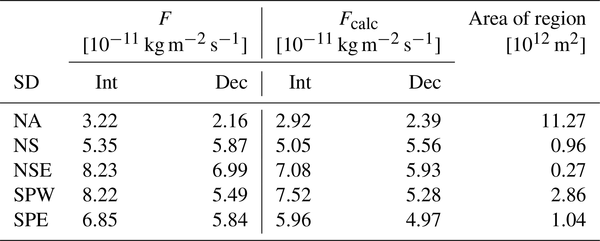
Archived climate model data available from CMIP6 on the ESGF nodes typically consist of monthly mean fields of physical, biological, and chemical parameters. These includes surface air–sea CO₂ fluxes from EC-Earth3-carbon cycle as well as ocean properties. The reproducibility of simulated integrated fluxes (F) derived from other parameters (Eqs. 1–3), particularly their variability across different timescales, provide a useful benchmark. It sets an upper limit on how much of the model variability we can expect to explain using physical quantities from archived monthly averages data. Figure 2 also shows the time evolution of F_calc (CO₂ flux calculated according to Eqs. 1–3) of a selected ensemble member (r4i1p1f1) and for the NS, NSE, and SPE region only. To accurately reproduce the simulated flux, F_calc is computed using a scaled wind speed. Since F_calc is derived from monthly mean values of all parameters, some of the short-term variability in dynamic factors – particularly wind speed – is smoothed out, leading to a lower mean wind speed compared to the daily mean used in EC-Earth3-CC. Hughes et al. (2012) discusses an averaging-related bias linked to ocean surface flux calculations and show that the use of monthly mean fields can introduce a bias into the mean flux estimates (also discussed by Esbensen and Reynolds, 1981; Simmonds and Dix, 1989; Gulev, 1994, 1997; Josey et al., 1995; Zhang, 1995; Esbensen and McPhaden, 1996; Simmonds and Keay, 2002). Given that Eq. (2) shows a nonlinear dependence of CO₂ flux on wind speed (U²), even small-scale wind variability can have a significant impact on flux calculations. To account for the reduced wind variability in the monthly mean fields and ensure consistency with the original flux calculation, a scaling factor of 1.2 is applied to the wind speed when computing F_calc. The scaled wind is only used for this calculation and not in any of the other analyses. It is also expected that the CO₂ flux variability is dependent on SST and SSS variability; however, the effect of SST and SSS on the solubility constant (K₀) is too small to be considered important in these calculations, and the SST and SSS components of Eqs. (1)–(3) is therefore not scaled. The absolute level of the F_calc compared to the model flux is well captured including the trend. For this ensemble, the correlation between the estimated flux and the model output in SPE exceeds 0.9 (R²) with a regression factor close to unity (1.1). We find comparable/significant skill in reproducing fluxes for the shorter timescale (not shown).

Figure 2 shows the average (weighted mean) CO₂ flux time series F for each region with interannual variability removed. The anthropogenic trend is evident in all regions including the accelerated trend after 1950. Differences between regions are evident with NSE showing the largest CO₂ uptake per unit area. Strong decade-scale variations do modulate regionally the accelerated trend after 1950 emphasizing the importance of ocean variability. Removing the anthropogenic trend and isolating interannual and decadal variability reveals (i) relatively comparable levels of variability across regions and (ii) a stronger variability on short timescales (Table 2). Ensemble mean results indicate that NSE, which is also the smallest area, is subject to strongest variability on both timescales, followed by the SPW (Table 2).

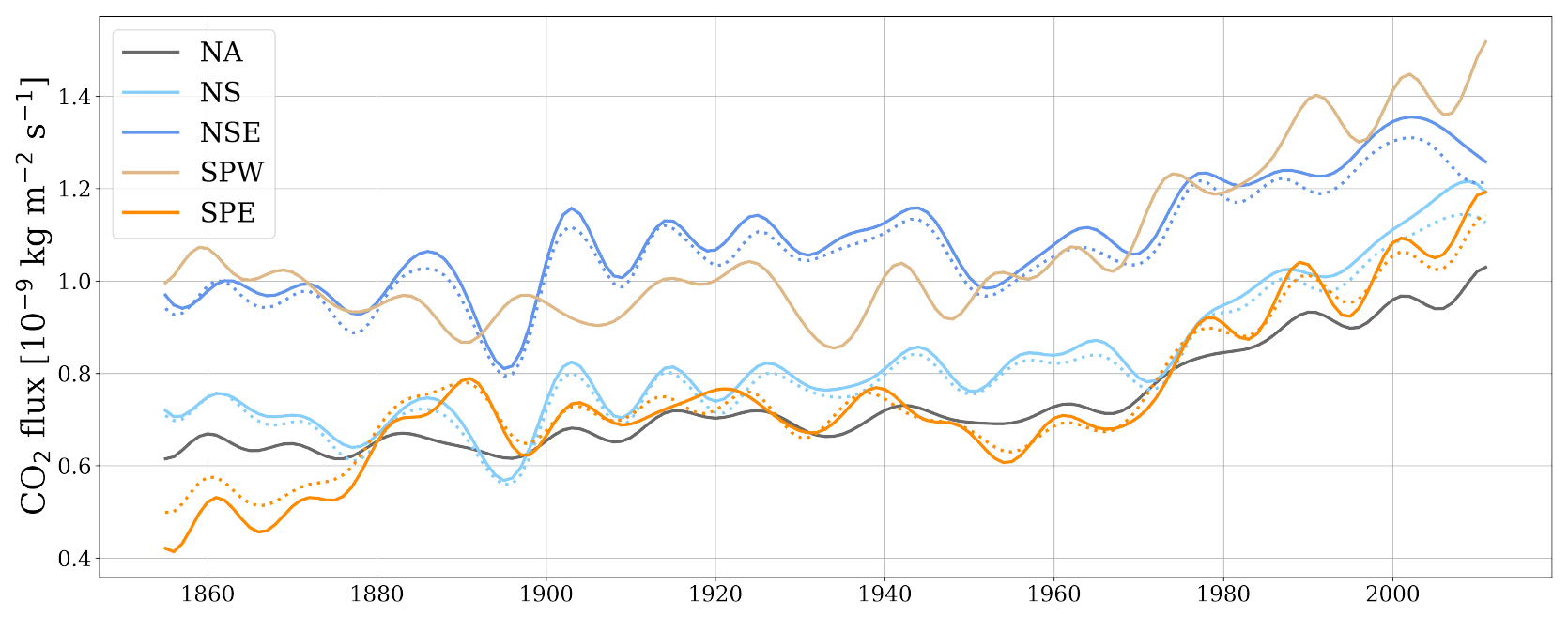
Figure 2 Decadal variability in the simulated CO₂ flux (F, solid line) and calculated flux (F_calc, dotted line) for ensemble member r4i1p1f1. Here the weighted mean is shown to compare the fluxes and variability across regions. F_calc only showed for NS, NSE, SPE.

3 Results

3.1 Regional CO₂ flux variability

To visualize the patterns of CO₂ flux variability across timescales and regions, we create composite maps of the CO₂ flux and the parameters we expect to be important drivers of the variability. These parameters include parameters already presented above (SST, SSS, SIC, ΔpCO₂, and wind); however, for the next part of the analysis we add MLD and sea surface height (SSH). These parameters represent larger-scale dynamics such as ocean circulation (SSH, gyre strength) and vertical mixing (MLD), which are candidates to be indirect processes controlling the CO₂ flux variability in EC-Earth3-CC. After detrending the data as described above, we define high and low CO₂ flux years in the different study regions based on the mean standard deviation (SD) for all the 10 members (±) one SD from the regional mean. The years are defined and selected for each member for all the parameters, where after the difference of the ensemble mean high minus low flux years is shown in composite maps (Figs. 3–7).

The NA region covers all the other regions. The CO₂ composite maps show a widespread homogeneous pattern of CO₂ uptake, intensified across the subpolar region (Fig. 3) and with regional differences. This includes the Irminger and Iceland Basins, where fluxes are moderated and locally reversed. On decadal timescales, positive values (increased CO₂ uptake) are confined to areas near the sea ice edge indicating that this exerts significant control over NA average CO₂ flux variability at longer timescales (Fig. 3b). On an interannual timescale, the widespread CO₂ uptake mirrors a widespread pattern of stronger winds and colder SST, indicating that these parameters are potential drivers of the CO₂ flux variability on shorter timescales. This is not the case for decadal variability where only positive wind speed project on regions of enhanced CO₂ flux, temperature generally warm and act to reduce solubility. A positive ΔpCO₂ pattern compares spatially with the positive CO₂ flux anomaly and negative SST anomaly (Fig. 3a). On the decadal timescale, a negative SSH anomaly, indicating a strengthening of the SPG, compares spatially with the positive CO₂ flux anomaly in the SPG region, which suggest that the strength of the SPG also could be a potential dynamical driver of the CO₂ flux variability, modifying key parameters like SST and SIC. The CO₂ flux variability pattern in the NA appears relatively homogenous, while its comparisons with other parameters are less distinct, except for SST on short timescales and SIC on long timescales. This suggests that multiple dynamics may be influencing CO₂ flux variability. To better understand these influences, we analyse smaller, well-defined regions to identify the key drivers of CO₂ flux variability.

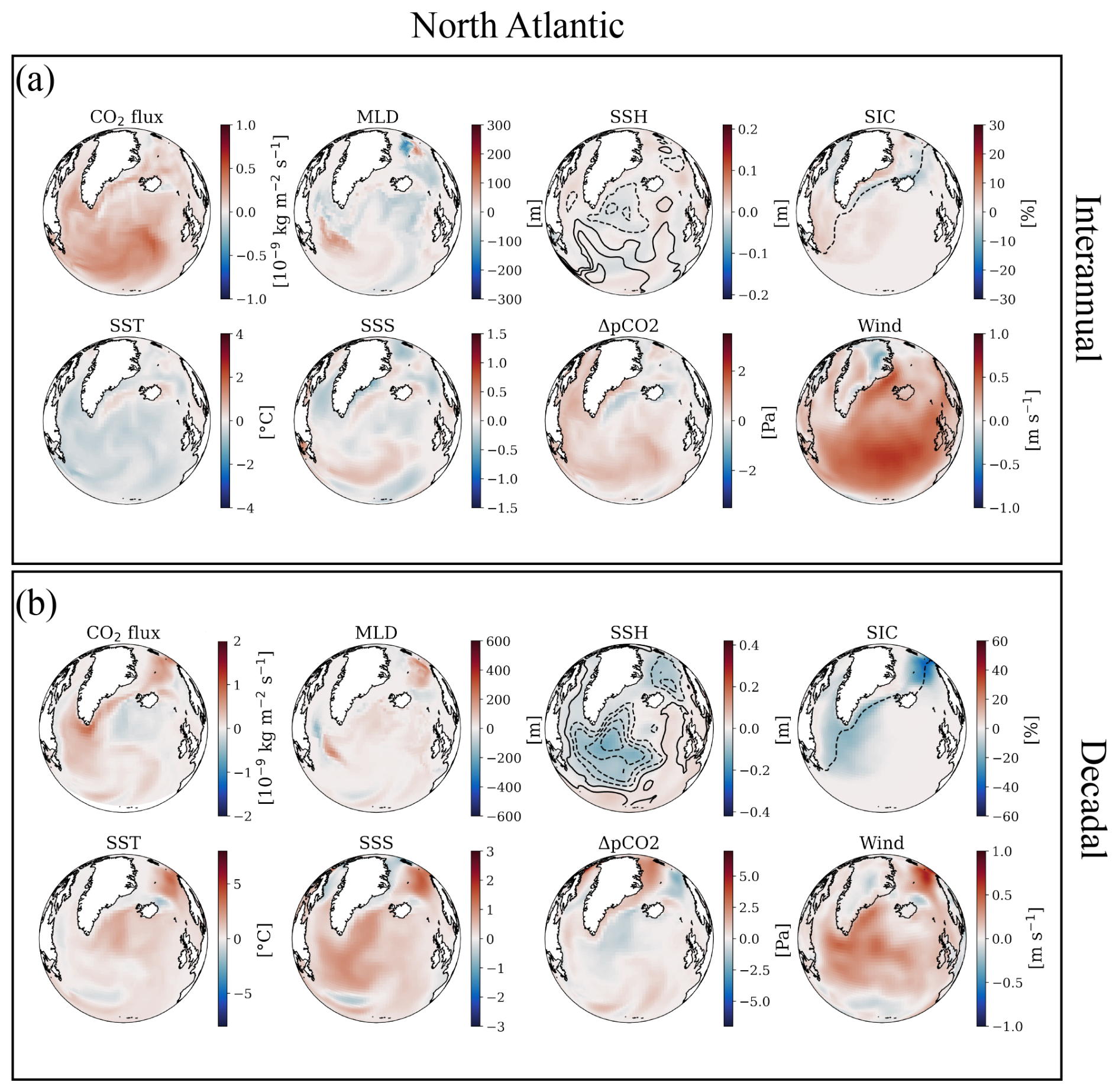
Figure 3 Anomalies of the high–low years of the dynamic parameters compared to the CO₂ flux anomaly in the NA. (a) showing interannual timescale and (b) showing decadal timescale. Full and dashed lines on top of the SSH anomaly shows the barotropic mass streamfunction anomaly and dashed line on top of SIC anomaly shows the 15 % SIC climatology (mean of 10 ensemble members on both timescales).

Focusing on the NS region, we see a widespread and homogeneous pattern of CO₂ uptake on an interannual timescale (Fig. 4), on short timescales confined to the NS, emphasizing the role of regional dynamical systems and need for a regional analysis. The NS shows the strongest flux anomalies across all the regions, in particular on long timescales. On decadal timescales, the CO₂ uptake is confined to an area of varying SIC in the NS with dynamical consistent patterns also in the SPG region, indicating that SIC is the main driver of the CO₂ flux variability in this region on longer timescale (Fig. 4a). Positive SST anomalies reaching 5 °C on a decadal scale would counteract the effects of sea ice variability. On the shorter timescale, the CO₂ uptake is enhanced across most of the NS region; however, on a decadal scale a small part of the region shows CO₂ outgassing (Fig. 4b), which is probably linked to the strong warming of the composite and reduced ΔpCO₂. Again, the positive CO₂ flux anomaly is perfectly confined to areas within an area of decrease in SIC, indicating that SIC is the main driver of CO₂ flux variability on the shorter timescale as well. The decrease in SIC is greater in the NS composite maps compared to the NA maps. On both timescales stronger winds compare spatially with the increased CO₂ uptake, similar to the NA region. However, the wind anomaly is stronger on the longer timescales compared to the shorter timescales. Following a decrease in SIC we see a deepening of the MLD due to increased convection, increasing the mixing and allowing for an increase in air–sea CO₂ flux. However, the small scale and spatial pattern associated with enhanced mixing is not obviously reflected in the patterns of CO₂ uptake. Also, from the spatial comparison of patterns, it is clear that ΔpCO₂ changes alone cannot explain the CO₂ flux variability.

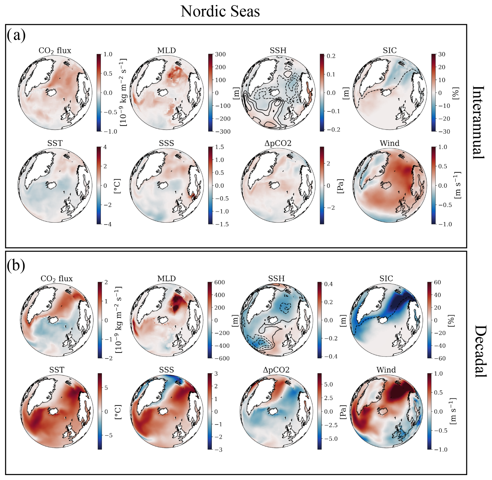
Figure 4 Anomalies of the high–low years of the dynamic parameters compared to the CO₂ flux anomaly in the NS. (a) showing interannual timescale and (b) showing decadal timescale. Full and dashed lines on top of the SSH anomaly shows the barotropic mass streamfunction anomaly and dashed line on top of SIC anomaly shows the 15 % SIC climatology (mean of 10 ensemble members on both timescales).

The NSE region represents the sea-ice-free part of the NS (less than 15 % SIC) and is in the path of the NA current crossing the Greenland Scotland Ridge. The composite maps of high minus low CO₂ flux years show an increased CO₂ uptake (Fig. 5) confined to the NSE region highlighting that our regionalization is relevant and allows us to isolate a dynamical regime. The region is confined by the 15 % SIC line, and shows a widespread positive CO₂ flux anomaly. Figure 5a illustrates that the interannual variability shows an increase in wind which compares spatially with a deepening of the MLD and an increase in the air–sea CO₂ flux. These patterns are more pronounced for the NSE than for the NS region. A decrease in SSH indicates a strengthening of the NS gyre circulation, the eastern part, mirroring an increase in MLD and CO₂ flux indicating a dynamic driver of the CO₂ flux variability. Figure 5b shows a confined pattern of CO₂ uptake, which compares spatially with a confined pattern of stronger wind, increased MLD as a result of a strengthening of the NS gyre (NSG; shallowing of the SSH), and increased SSS. Compared to the NA region, the NSE gives a clearer indication of the driving forces behind the CO₂ flux variability.

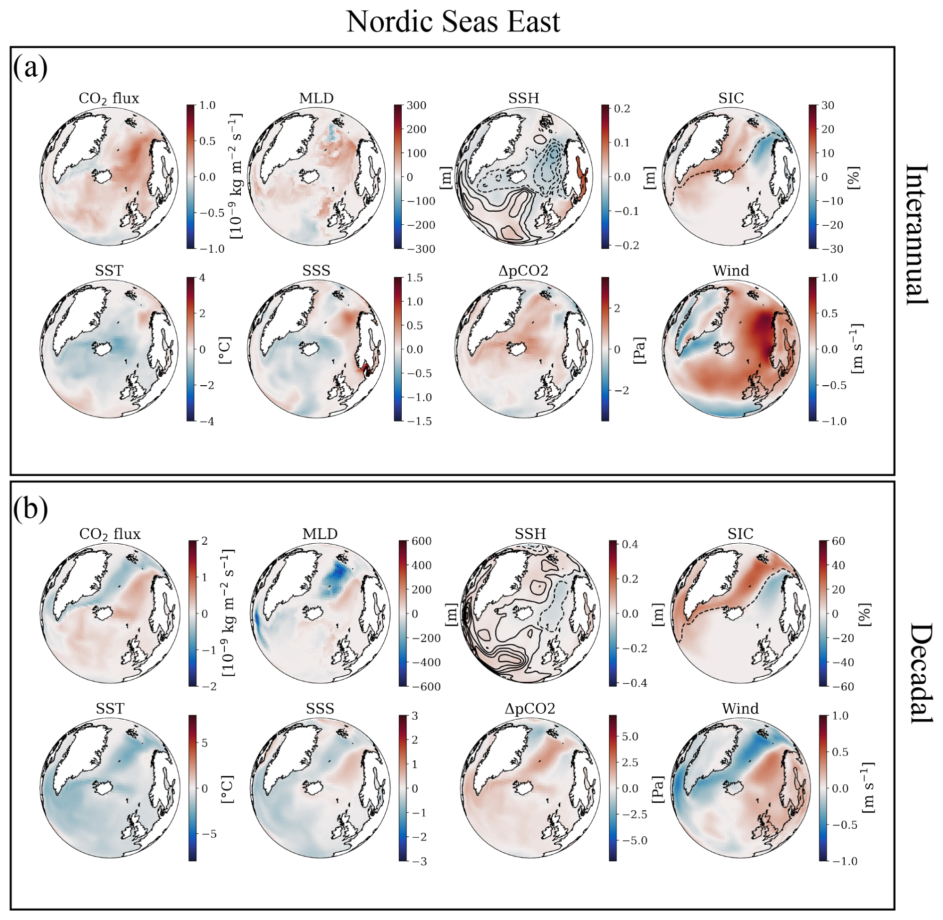
Figure 5 Anomalies of the high–low years of the dynamic parameters compared to the CO₂ flux anomaly in the NSE. (a) showing interannual timescale and (b) showing decadal timescale. Full and dashed lines on top of the SSH anomaly shows the barotropic mass streamfunction anomaly and dashed line on top of SIC anomaly shows the 15 % SIC climatology (mean of 10 ensemble members on both timescales).

In the western part of the subpolar region, the CO₂ flux spatial pattern is strikingly similar to the pattern we can construct for the entire NA on both timescales (Figs. 3 and 6). This can in part be expected from the vast area of the region hereby dominating the area-averaged fluxes and composites. Key differences with the NA region include the Irminger Sea where also SSH patterns indicate a dynamical separation on interannual scales. On the interannual timescale the region shows CO₂ uptake within the full region (Fig. 6a), whereas the decadal CO₂ flux shows both positive and negative anomalies within the region (Fig. 6b). In general all the parameters show similar patterns to the NA on both timescales. However, on the interannual timescale we see a more clear and confined signal from SST and SSS compared to the NA. A negative SST anomaly compares spatially with increased CO₂ uptake in the full region, whereas a positive SSS anomaly in most of the region shows a relationship with the CO₂ flux variability, emphasizing how the SSS can work as an indirect driver or indicator. On the decadal timescale we see a clear and confined signal in the indicated drivers of the CO₂ flux compared to the NA region. Here, we see that the CO₂ uptake is confined within the region of decreasing SIC, indicating that SIC forces a main control on the CO₂ flux variability in the region. Furthermore, we see a greater strengthening of the SPG as indicated by the decrease in SSH on both timescales; however, the strongest signal is seen on the longer timescale, where we also see a shift towards the east as expected in a strong SPG phase. The strengthening of the SPG results in a deepening of the MLD and introduces more saline Atlantic water into the system from further south, which explains why we see a positive SSS anomaly and increased CO₂ uptake. As in the NA region, we see opposite anomalies for the SST on the two timescales. A negative SST anomaly mirrors a positive CO₂ flux anomaly on the short timescale, whereas on the longer timescale, we see a positive SST anomaly and a positive CO₂ flux anomaly.

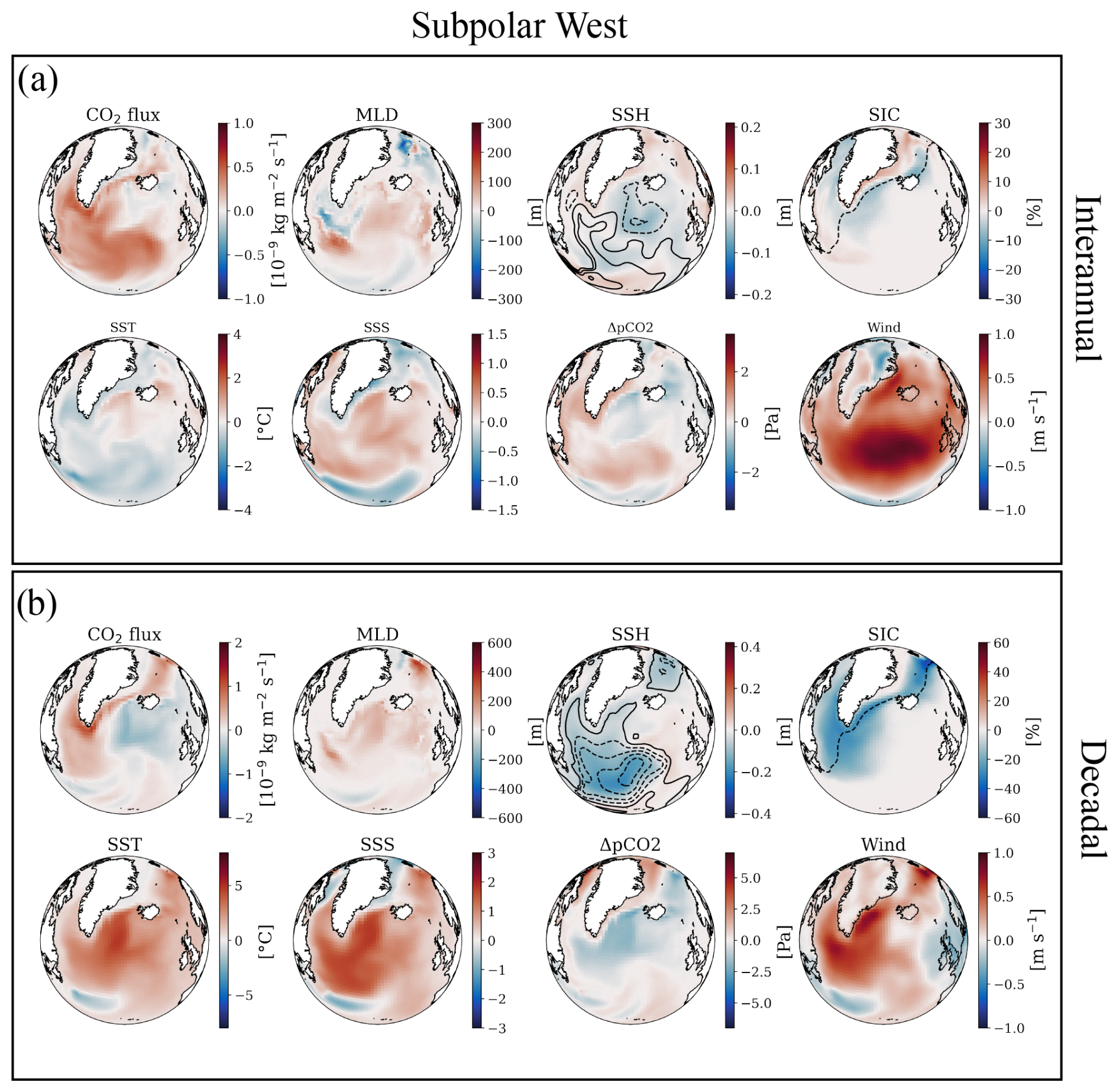
Figure 6 Anomalies of the high–low years of the dynamic parameters compared to the CO₂ flux anomaly in the SPW. (a) showing interannual timescale and (b) showing decadal timescale. Full and dashed lines on top of the SSH anomaly shows the barotropic mass streamfunction anomaly and dashed line on top of SIC anomaly shows the 15 % SIC climatology (mean of 10 ensemble members on both timescales).

Finally, we look at the eastern part of the subpolar region (Fig. 7). The composite maps show patterns of increased CO₂ uptake, which is regionally well confined to the eastern SPG and not apparently analogous to the composite patterns derived for SPW. This also includes the NA region. On the interannual timescale SSH reflects what may best be characterized as a relative blocking of the path of the NA current (a closed gyre system building up sea surface height). On the decadal timescale this blocking cell is located farther south, outside the SPE region, but in both cases results in cooling of the wider subpolar region as well as freshening. Despite these basin-wide linkages, the CO₂ flux changes are regionally exaggerated in the SPE. Not surprisingly, the dynamical changes – a blocking of the path of the NA current – are also characteristic of the composite maps for the NSE region (Fig. 5). Despite this apparent similarity, the CO₂ flux patterns in both cases do not extend across the Greenland Scotland Ridge. This may be explained by phase differences in the effects.

The spatial pattern of positive CO₂ flux anomaly reflects a shallowing of the MLD on the interannual timescale. This cannot directly be linked to increased uptake, as described in Sects. 1 and 3.1, as a shallowing of the MLD is related to a less ventilated water column, and thereby a decrease in the CO₂ uptake. This link is discussed further in the next section. Also on the interannual timescale, a positive wind anomaly, and a negative SST and SSS anomaly also align spatially with positive CO₂ flux anomalies. On the decadal timescale, the signals from the MLD and wind are less clear; however, a negative SST and SSS anomaly compares spatially with the increased CO₂ uptake in the region.

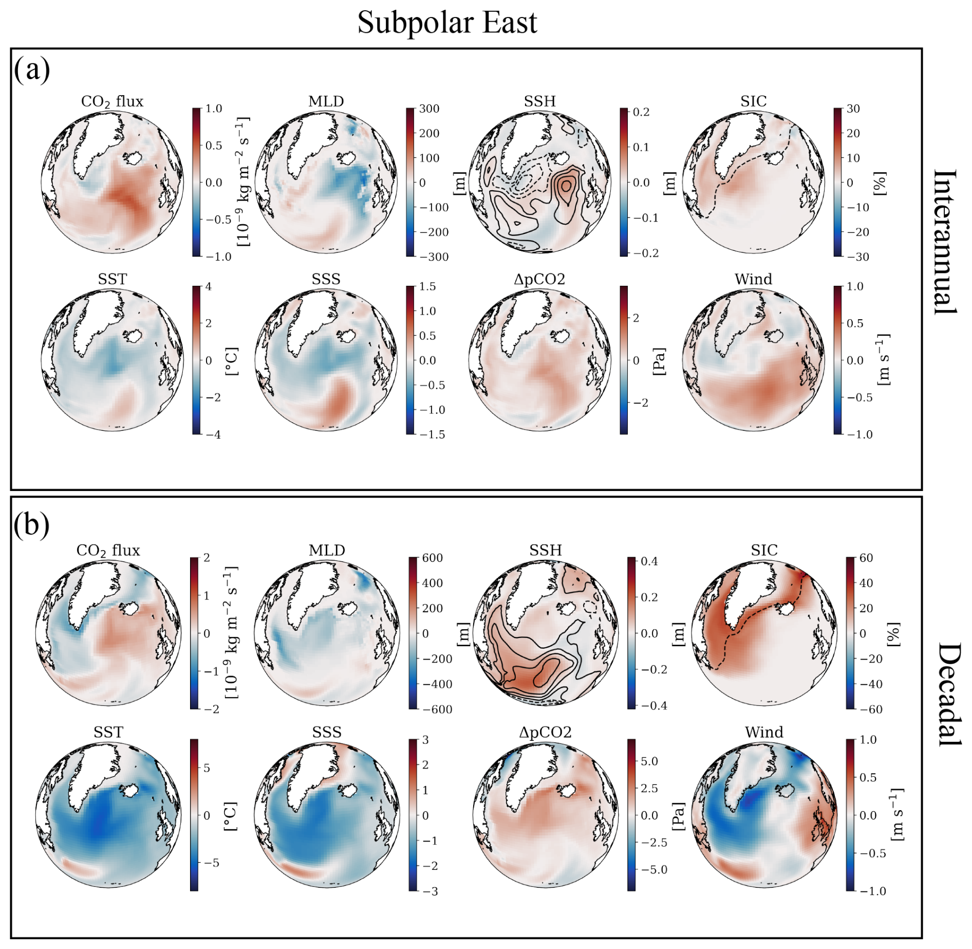
Figure 7 Anomalies of the high–low years of the dynamic parameters compared to the CO₂ flux anomaly in the SPE. (a) showing interannual timescale and (b) showing decadal timescale. Full and dashed lines on top of the SSH anomaly shows the barotropic mass streamfunction anomaly and dashed line on top of SIC anomaly shows the 15 % SIC climatology (mean of 10 ensemble members on both timescales).

3.2 Ocean indexes

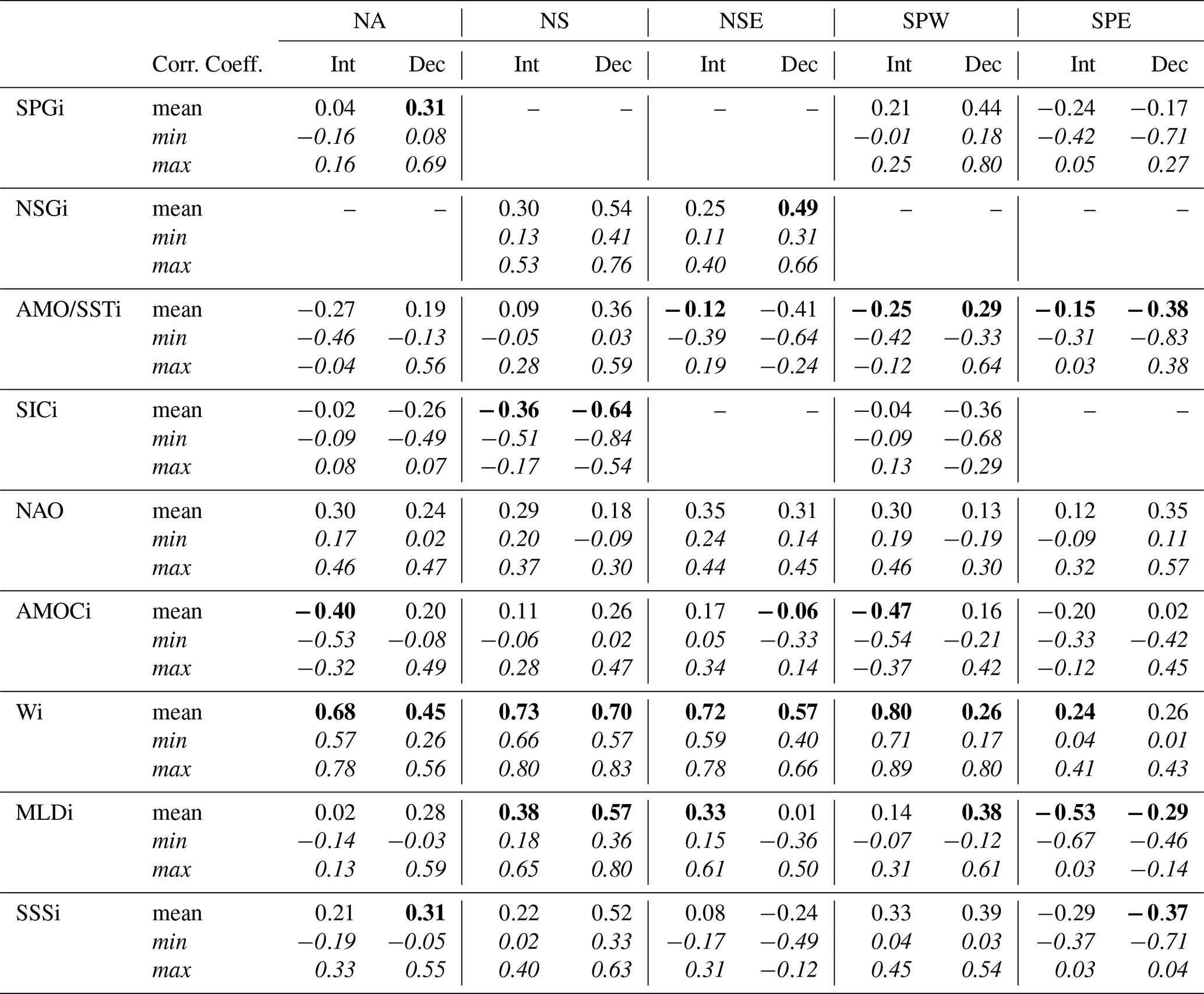
Following the qualitative discussion of the relationship between the CO₂ flux variability and the dynamical parameters on different timescales, we define integrated quantities and make use of ocean indicators such as the SPG index to understand the statistical significance of the identified relationships between the CO₂ flux and ocean variability (Table 3).

The SPG index (SPGi) is here defined simply as the minimum SSH of the NA region. This differs from other definitions (Hátún et al., 2005; Berx and Payne, 2017) but captures the main variability of the Earth system model analysed. The index is inverted, meaning that a positive (negative) anomaly indicates a strong cyclonic (weak) SPG. The SPG index describes not only the state of the subpolar region but observations also shown to characterize variability in water mass properties at the gateways to the NS (Hátún et al., 2005, 2017). As such, the SPGi may be linked to CO₂ flux variability directly by describing the extent of the characteristic colder and fresher subpolar upper ocean water masses and indirectly through correlations with other drivers such as variability in sea-ice margins, wind stress, and ocean mixing locally and remotely (NS). From correlation coefficients (zero lag) between the SPGi with the CO₂ flux anomaly for the different regions (NA, NS, NSE, SPW, SPE), listed in Table 3, it is clear that the SPGi does not explain the CO₂ flux variability on the interannual timescale very well, though reassuringly the highest correlations are found for the SPW region. The SPGi correlates better on the decadal timescale, with an ensemble mean of 0.31 and 0.44 in the NA and SPW, respectively. Several ensemble members show a correlation coefficient of 0.4 or higher in both regions, but a few ensemble members show very low correlation, resulting in reduced ensemble mean values. The SPE shows a large spread in individual ensemble correlations with both positive and negative correlations, resulting in an ensemble mean of −0.24 and −0.17 (interannual and decadal, respectively). The low degree of correlation on both timescales is expected in part due to the findings from the composite map analysis of a more regional SSH (and streamfunction) “blocking pattern” of the NA Current.

The NS gyre index (NSGi) is defined as the minimum SSH in the NS region, similar to the SPGi. The index is inverted, meaning that a positive value indicates a strong cyclonic gyre circulation, whilst a negative value indicates a weakening of the gyre circulation. The NSGi is modulated by changes in wind stress curl and also is not independent of other possible indices defined on the basis of MLD and SIC. We have no a priori expectation of a strong relation between the NSGi and CO₂ flux in other regions. The NSGi correlates well with the CO₂ flux variability in the NS on the decadal timescale (0.54, Table 3), but also on the interannual timescale (0.30, Table 3). A strong (weakened) NSGi results in an increased (decrease in) CO₂ uptake in the ocean. Hátún et al. (2021) show that a strong NSG circulation results in an uplifted thermocline, which results in more ventilation of deeper water. The ventilation of deeper water could lead to an increased air–sea CO₂ flux, and work as a driver for the increased CO₂ uptake in the NS. The composite maps show a strengthening of the NSG (deepening of the SSH) on both timescales; however, a greater strengthening on the decadal timescale indicates that a strengthening of the NSG could result in an increased atmosphere–ocean CO₂ flux.

The AMO index is defined as the anomaly of the mean SST in the NA region. For the regions within the NA, the index is defined as an SST index, which is the anomaly of the mean SST within the region. We have chosen to use the SSTi for the smaller regions, to investigate the direct relationship of SST and CO₂ flux variability within the regions. A positive AMO/SSTi phase describes a warming of the NA. As higher SST's increase the pCO₂ in the ocean due to lower solubility, the AMO should be negatively correlated to the CO₂ flux. However, Breeden and McKinley (2016) show how a positive AMO phase results in a decrease in DIC in the SPG, which decreases the solubility and increases the fCO₂ (and the pCO₂). On the decadal timescale we see that the CO₂ flux variability in the NS and SPW region correlates positively (0.36 and 0.29, Table 3) with the SSTi, which can be related to the dynamics explained by Breeden and McKinley (2016). Also, an increase in temperature in the NS would result in a decrease in SIC, allowing for an increase in CO₂ flux. Breeden and McKinley (2016) state that SST and the solubility of CO₂ in the ocean still affects the pCO₂ in the ocean (and thereby the air–sea CO₂ flux), but that the biogeochemical dynamics, such as DIC is of a stronger amplitude. The NSE and SPE regions shows an inverted correlation between the CO₂ flux variability and the SSTi on both timescales (NSE: −0.12 and −0.41 SPE: −0.15 and −0.38, interannual and decadal), indicating that the temperature effect on the CO₂ solubility in the surface ocean dominates the CO₂ flux variability in these regions (Table 3). In the NA the degree of correlation varies a lot between the ensemble members from a negative/weak correlation to a stronger correlation, which makes it difficult to say anything in general about the full NA region.

The sea ice index (SIi) is defined as the SIC anomaly in the specified regions. An increase in SIC results in a decrease in CO₂ flux into the ocean in case no other factors are changing. In the NS the SICi in general has a strong negative correlation with the decadal CO₂ flux anomaly, all of the members showing a correlation coefficient above 0.50, resulting in an ensemble mean of −0.64 (Table 3). The interannual variability in the NS shows a lower correlation, with an ensemble mean of −0.36 (Table 3). On both timescales, the SPW region shows a weaker negative correlation compared to the NS (−0.04 and −0.36, interannual and decadal), as expected due to a smaller degree of sea ice extent in the SPW. However, it is clear that the SIC is still dominating the CO₂ flux variability in this region. The NA region shows the weakest correlation between the SICi and the CO₂ flux variability, which might be explained by the fact that the sea-ice-covered region of the NA is small (−0.02 and −0.26 interannual and decadal). The SICi has not been applied to the NSE and SPE regions, as they are more or less sea ice-free.

The NAO index is defined as the atmospheric surface pressure level anomaly between Iceland (65° N, 20° E) and the Azores (40° N, 25° E) in the winter months (djfm; Hurrell, 1995). The correlation between the NAO and CO₂ flux is in general strongest on the interannual timescale, showing a correlation coefficient of approximately 0.3 for most regions, except SPE that shows 0.12 and 0.35 interannual and decadal, respectively. On the decadal timescale the ensemble mean correlations are weaker; however, in particular in the ice-free SPE and NSE and in the NA some ensemble members show a correlation of 0.4–0.5 (Table 3). The NAO and associated wind stress and wind stress curl affect the ocean dynamics of the region including sea ice distribution which may explain the positive correlations, whereas the direct effects of changes in wind stress on gas transfer would be expected to result in negative correlations for some regions.

The AMOC index (AMOCi) is defined as the anomaly of the maximum of the model Atlantic Meridional Overturning Circulation (streamfunction) at 45° N in the top 1000 m of the water column. We choose 45° N to align with the boundary of the subpolar and subtropical gyres and reduce potential time lag, that would follow from using an index defined at lower latitudes. On the interannual timescale, the AMOCi shows a strong negative correlation in the NA and SPW regions (−0.40 and −0.47, Table 3), indicating that a weakened AMOC resulting in less heat transport to the northern NA will result in increased ocean CO₂ uptake. In the other regions, the ensemble members show a low correlation on the short timescale. On the decadal timescale, somewhat surprisingly, the AMOCi is not as closely and directly related to surface CO₂ exchange with both negative and positive correlation coefficients in all the regions, resulting in a weak average correlation (Table 3).

The wind index (Wi) is defined as the anomaly of the average near surface (10 m) wind speed in the different regions. As expected based on Eq. (2), the Wi correlates positively with the CO₂ flux variability for all regions independent on timescale. On both interannual and decadal timescale, the Wi shows a high correlation with the CO₂ flux in the NA (0.68 and 0.45), NS (0.73 and 0.70) and NSE (0.72 and 0.57, Table 3). However, SPW only shows a high correlation on an interannual timescale (0.80 and 0.26 decadal), whereas SPE shows a weaker correlation on both timescales (0.24, 0.26). In the composite maps all the regions show a strong positive wind anomaly, whereas the SPE region shows a weak positive anomaly on the interannual timescale and a mix of negative and positive anomalies on the decadal timescales, which might explain the weak correlation seen in the region.

To understand the dynamic process of upper ocean mixing and its effect on the atmosphere–ocean CO₂ flux variability a MLD index (MLDi) is defined based on the anomaly of the MLD max value of the different regions. The MLDi shows a strong negative correlation in the SPE (0.53 interannual; 0.29 decadal, Table 3) on both timescales, and a strong positive anomaly in the NS (0.38 interannual, 0.57 decadal) indicating a complex, indirect, and regionally different linkage. Spatial patterns of MLD show some resemblance to ΔpCO₂ in the SPE with an inverse relation (Fig. 7), which can be explained by shoaling of the mixed layer leading to less ventilation of DIC rich deeper layers and thus increased ΔpCO₂.

Salinity directly, but weakly influence the gas transfer (Eq. 1), but we choose to also define the SSS index (SSSi) as preliminary analysis showed a clear correlation between PP and SSS in the EC-Earth3-CC output data which can be exploited to be able to use the analysis from this study on different Earth system models that might not include a biogeochemical component in possible future studies. Furthermore, the SSS dynamics also translates to the strength of the SPG, the melting of sea ice, and transports of different water masses in the NA. We have defined the SSSi as the SSS anomaly in the different regions. The SSSi shows the strongest interannual correlation in the SPW (0.33), and the strongest decadal correlation in the NS (0.52) and SPW (0.39). In the composite map of the NS region, we see a strong positive SSS anomaly correlating with a positive CO₂ flux anomaly (Fig. 4). The SSSi shows a strong negative correlation with the CO₂ flux in the SPE, which is also evident in the composite maps (Fig. 7).

Table 3 Index analysis. Correlation coefficients are the mean of 10 ensemble members in interannual (int) and decadal (dec) timescales. In cursive min and max values for individual members are shown to indicate spread (uncertainty) of the index analysis. In bold parameters used for regression models in Sect. 3.3.

3.3 Regression analysis

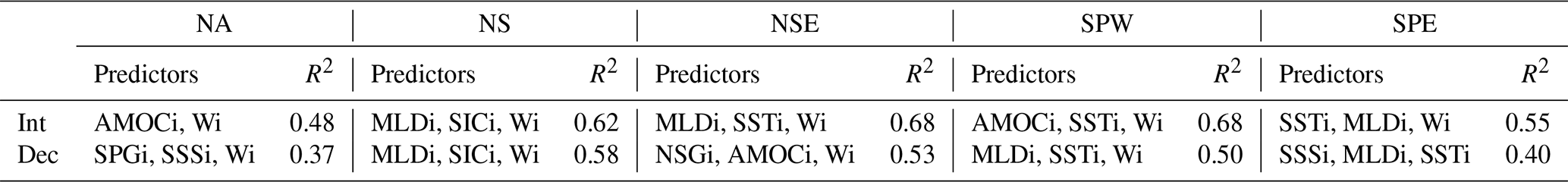
A regression model has been set up for each of the regions and both timescales, based on the findings from the composite maps and the index correlation analysis. The predictors chosen for the regression models have been chosen to provide the best possible regression model, not only focusing on the linear relationship between the predictors and the CO₂ flux as shown in the index analysis (Table 3). Some predictors might show a weak correlation coefficient, but contribute to a higher degree of explanation in combination with other predictors. For instance the NAO index is not considered for the regression models, as it to some degree represents the same dynamics as the Wi, and therefore does not contribute to a higher degree of explanation for the regression models. In the following, the descriptions of the regression models are based on the mean R² value of the 10 ensemble members for each region (Table 4). The regression models for the interannual variability shows slightly higher correlation/explanation for the CO₂ flux variability in the different regions compared to the decadal variability. In general, the NA region shows the lowest degree of correlation on both timescales, emphasizing the need to divide the region into smaller regions.

The interannual CO₂ flux variability in the NA region can be explained by variability in AMOC and wind speed, with an R² value of 0.48 (Table 4). The spatial patterns show a strong, homogeneous positive wind anomaly that correlates well with a positive CO₂ flux anomaly in the NA (Fig. 3). Furthermore, the index analysis shows that both the AMOCi and Wi correlate well with the CO₂ flux variability (0.40 and 0.68, respectively, Table 3). The wind speed is expected to be driving the CO₂ flux variability, but the AMOCi represents a more dynamic control on the variability. The decadal timescale regression model includes predictors such as SPGi, SSSi, and Wi. Here, the R² value is 0.37 (Table 4). The composite map does not show a strong spatial pattern between the predictors and the CO₂ flux variability, which might explain the lower R² value. The predictors chosen for the decadal regression model align with the indexes with the greatest correlation as seen in Table 3.

The NS region shows a good degree of correlation (0.62 and 0.58 for the interannual and decadal timescales respectively, Table 4) based on MLDi, SICi, and Wi. The sea ice concentration works as a main driver for the CO₂ flux variability in the NS as discussed earlier and seen in Fig. 4. Furthermore, a strong positive signal in the MLD anomaly correlates with the CO₂ flux anomaly, indicating that dynamical processes, such as strengthening of the NSG (a deepening of the SSH) and increased convection related to disappearing sea ice also controls the CO₂ flux variability in the NS. The index correlation analysis also indicates the wind stress as a controlling parameter in this region in both timescales (Table 4). The fact that the regression model is based on the same parameters for both timescales indicates that the processes driving the CO₂ flux variability are stable across timescales for this region.

The NSE region shows a high degree of correlation as well (0.68 and 0.53 interannual and decadal respectively, Table 4). The interannual predictors being MLDi, SSTi, and Wi and the decadal NSGi, AMOCi, and Wi. The interannual and decadal variability is well explained by the spatial patterns in the region (Fig. 5). However, the index analysis show a weak linear correlation between the predictors SSTi and AMOCi and the CO₂ flux on the interannual and decadal timescale, respectively (Table 3). The low correlation coefficient in the index analysis does not, however, rule out, that the SST and AMOC contribute to the variability combined with other predictors, as shown in the regression models for the region. The NSE regression models show that dynamical processes such as ocean mixing and circulation drive the CO₂ flux variability within the region in addition to physical parameters such as SST and wind, which is expected from the gas transfer equations (Eqs. 1–3).

The western part of the subpolar region shows the next best degree of correlation on the interannual timescale (0.68 interannual and 0.50 decadal, Table 4). The regression model set-up is based on the interannual variability entails AMOCi, SSTi, and Wi and shows an R² value of 0.68. Based on MLDi, SSTi, and Wi the regression model for the variability on the decadal timescale shows an R² value of 0.50. We expected dynamic ocean processes such as SPG strength to control the CO₂ flux in the region; however, the regression model shows that the AMOCi and MLDi are predictors representing the dynamic ocean processes. The SST anomaly shows a negative anomaly on the interannual timescale and a positive anomaly on the decadal timescale, both correlating with a positive CO₂ flux anomaly (Fig. 6), which is also evident in the negative and positive correlation of the SSTi in the index analysis on interannual and decadal timescales, respectively (Table 3). This shows that the relationship between the predictors might not be linear, and that they, in combination, contribute to the CO₂ flux variability even though they individually do not contribute.

Finally, the CO₂ flux variability in the SPE region is controlled by SST and MLD on both timescales; however, the interannual regression model also includes Wi, and the decadal regression model includes SSSi, as indicated in Fig. 7. The R² values of the regression models show that the correlation is better on the interannual timescale (0.55) than the decadal timescale (0.40) (Table 4). Here, the regression model analysis shows that in addition to expected drivers such as SST and SSS (as discussed earlier and based on Eqs. 1–3), dynamical processes such as ocean mixing also drive the CO₂ flux variability. The MLD variability points to the SPE being a dynamical region, possibly affected by the SPG circulation in the western part of the subpolar region. Furthermore, SPE is an ice-free region, allowing us to understand the dynamics of the CO₂ flux variability without the strong SIC driver. The decadal regression model for the SPE is the only one not including Wi. The wind speed anomaly is both negative and positive within the region, which indicates that the wind speed might not be a controlling factor in the SPE (Fig. 7).

Table 4 Applied regressions for all regions across timescales. R² values based on mean R² for all 10 ensemble members in interannual (int) and decadal (dec) timescales.

4 Discussion

4.1 Biases in Earth system models

We calculated the CO₂ flux using the dependent parameters from the model as seen in Eqs. (1)–(3) to test to what degree the model CO₂ flux could be reproduced. Using monthly mean fields of SST, SSS, ΔpCO₂, and wind speed we are able to reproduce the CO₂ flux variability; however, to reproduce the total flux we need to use a scaled wind field (wind ×1.2). PISCES calculates the air–sea CO₂ flux daily (Döscher et al., 2022; Aumont et al., 2015), and by using monthly mean fields (using available data) we risk a smoothing of the actual daily variability that can explain the need for a scaled wind field. Turner et al. (1996) discusses how using monthly mean fields for wind and temperature can affect the calculation of atmosphere–ocean fluxes (in their study dimethyl sulfide fluxes in the NS; however, using Wanninkhof (1992) gas transfer equations as in this study, Eqs. 1–3). Reproducing the CO₂ flux helps us understand the sensitivity and dependencies on the physical parameters used to calculate the flux. The wind speed field shows a big sensitivity, which is also emphasized in the regression models, all but one entailing the Wi.

Earth system models inevitably simplify the complex climate system, which will introduce biases to the modelled processes. One example being the monthly mean wind field that introduces a bias in the calculated CO₂ flux. Another bias addressed in this paper is the SIC bias in EC-Earth3-CC. As stated by Döscher et al. (2022), Tian et al. (2021) and shown in Fig. 1b EC-Earth3 (and thereby EC-Earth3-CC) shows an overestimation of the SIC in the NS and the NA. The index and regression model analysis of the NS shows that SIC is a driver of the CO₂ flux variability, as expected based on Eq. (3). Therefore, the overestimation of sea ice extent and concentration in EC-Earth3 will undoubtedly affect and possibly control the CO₂ flux variability in the ocean in the EC-Earth3-CC runs. However, even in regions of sea-ice such as the SPW and the NA, SIC does not exclude significant effects of other processes, as SIC is not regarded as a predictor for the CO₂ flux variability in these regions (Tables 3, 4).

4.2 Predictors

Our analysis demonstrated that the CO₂ flux variability and its drivers cannot be assessed meaningfully considering the larger northern NA region; but instead needs to be stratified at a regional and sub-basin level. Our analysis shows a high degree of explained variability of the CO₂ flux within the regions defined including dynamically separated ocean regions (Table 4). Based on the regression models we have established, it is clear that a linear correlation between the CO₂ flux and other predictors will not allow us to explain and understand the full CO₂ flux variability. It is clear that internal dynamics between the different predictors also affects the CO₂ flux variability as shown in Sect. 3.3. Furthermore, we also establish that not only the physical parameters SST, SSS, and wind speed work as drivers of the CO₂ flux in the regions. It is evident that wind speed poses a great control on the CO₂ flux variability as discussed earlier, but we also see dynamic predictors such as ocean mixing (MLDi), gyre circulation (NSGi/SPGi), and larger-scale ocean circulation and transport (AMOC) as drivers. Holliday et al. (2020) and Hátún et al. (2005, 2017) discuss how the larger-scale dynamics such as the gyre circulation (SPG and NSG) and AMOC variability affect the SST, SSS, and PP in the northern NA, aligning with our findings. Despite being the smallest region in terms of area among these studies (Table 2), the NSE region exhibits the highest variability and mean flux. This remains the case until 1960 (Fig. 2), when the SPW and NSE flux time series converge. Our regression analysis yields the highest R² values in the NSE and SPW regions (Table 4), underscoring the robustness of our approach. Notably, the fact that our regression models provide the strongest explanatory power in the regions with the greatest variability and mean CO₂ flux suggests a stable and reliable representation of the system dynamics.

Throughout our analysis we have established that a deepening of the MLD often coincides with a positive CO₂ flux anomaly, which in some cases can be explained by a deepening of the MLD resulting in an increase in DIC in the surface layer, decreasing pCO₂ in the surface layer and thus increasing the atmosphere–ocean CO₂ flux (Figs. 3–6). However, we also see the deepening of the MLD as a response to a decrease in SIC, resulting in convection and an increase in the atmosphere–ocean CO₂ flux, which is especially evident in the NS region (Fig. 4). The index analysis also shows a positive correlation between MLD and CO₂ flux in all the regions except for the SPE (Table 3). However, counter-intuitively to what is earlier established in our composite map analysis, we see a (strong) negative correlation between MLD and the CO₂ flux, both spatially and in the index analysis in the SPE region as mentioned (Fig. 7, Table 3). The MLDi is one of the predictors defining the regression models for both timescales in the SPE, which means that the MLD variability explains a big part of the CO₂ flux variability, despite their counter-intuitive negative correlation. The spatial patterns of the SPE shows a negative mirroring between the CO₂ flux and both SSS and SST most evident on the longer timescale, but also to some degree on the short timescale (Fig. 7). Furthermore, the spatial patterns also show a possible blocking of the NA current, indicated by a closed gyre system building up SSH. The blocking of the NA current might allow for fresh, cold, and nutrient-rich Arctic water to enter the system, resulting in a positive CO₂ flux anomaly due to a decrease in temperature and nutrient supply increasing the PP and thus the CO₂ uptake. Increased freshwater supply from the Arctic would also result in increased stratification of the water column, indicated by the shallowing of the MLD and thereby the negative correlation between the CO₂ flux and MLD. We have also found that in EC-Earth3-CC, PP, and SSS are more or less replaceable, including spatial patterns and their correlation. The NA is strongly influenced by the AMOC and SPG circulation, both regulating the salinity distribution and nutrient transport. The change in SSS reflects changes in the balance of freshwater input (i.e. freshwater from the Arctic). Both SSS and PP are sensitive to these large-scale circulation dynamics, and they might co-vary, making them somewhat interchangeable in Earth system models. These observations indicate that CO₂ flux variability in the northern NA cannot be adequately explained by individual predictors in a linear framework. Instead, a comprehensive understanding of the underlying processes and the interactions among predictors is essential to accurately capture atmosphere–ocean CO₂ flux variability.

4.3 Future projections

Based on the results of our regression model analysis we expect that the regression models are also robust for assessing the CO₂ flux variability and tendencies in the NA from scenario simulations without a CC (EC-Earth3). This would be beneficial for estimating uncertainties related to future CO₂ uptake and in general to understand the CC effects of regional climate change patterns. We have purposely defined the regression models by using non-biogeochemical predictors only. Studies have looked into the predictability of interannual-to-decadal variability: Li et al. (2016) show a predictive skill of CO₂ uptake in the western SPG of up to 4–7 years based on an Earth system model prediction system. They conclude, that the predictive skill is attributed to the combination of improved ocean physical states and circulation variability, primarily in winter which corroborates our approach. Ilyina et al. (2021) shows a predictive skill for the global ocean carbon sink of up to 6 years for some Earth system models. Further motivation for focussing on dynamical indices comes from Fransner et al. (2020). They show that the predictability of ocean carbon uptake correlates well with the predictability of the MLD, suggesting that the predictable signal comes from exchange of DIC with deep waters.

Looking into the near future, studies consistently establish that the warming of the global climate system is also manifested in warming of the ocean (Fox-Kemper et al., 2021; Bopp et al., 2013; Fu et al., 2016; Laufkötter et al., 2016; Liu et al., 2023; Kwiatkowski et al., 2020). Ocean temperature increase would from first principles result in a decreased atmosphere–ocean CO₂ flux through the effects on solubility; however, as demonstrated in this study the CO₂ flux variability is more complex than simple linear relationships with temperature. For example, an increased ocean temperature will lead to a melting of the sea ice in the northern NA, resulting in more open ocean surface that can take up CO₂. However, a warming ocean will also affect the ocean circulation, both the large-scale circulation and the small-scale ocean mixing. AMOC is predicted to slow down with global warming (McKinley et al., 2023; Liu et al., 2023). Stagnating ocean circulation in the NA will, as seen in our analysis, affect the CO₂ flux variability, in particular the SPW region of the NA, but also further north in the NSE region. Furthermore, a warming ocean combined with melting ice and stagnated ocean circulation could result in increased upper ocean stratification, reduced MLD, and less exchange with high DIC water masses in the deeper ocean. The predicted global warming will possibly result in stronger winds in the NA region (Lee et al., 2021; Ruosteenoja et al., 2019) which, based on the gas exchange equation and our results, will contribute to increasing the atmosphere–ocean CO₂ flux. Our results identify SIC and wind speed as main drivers of the CO₂ flux variability in a number of subregions of the northern NA, which would indicate an increase in ocean CO₂ uptake in the near future but counteracted by the direct temperature effect.

To expand the regression analysis to investigate their robustness in scenario runs using other Earth system models it is pivotal to have an in-depth understanding of the model set-up and of the characteristics of indices in the specific model including biases and variability. Examples that might complicate the applicability of the regression models from this study could be how the gas transfer is handled across sea ice, how realistic the separate indices are compared to observations, and how the indices relate to each other. Our analysis provides a framework for identifying the key predictors and processes driving atmosphere–ocean CO₂ flux variability in the northern NA, but further work is necessary before applying the framework across other Earth system models. We demonstrate that physical ocean and atmospheric parameters alone account for a significant portion of this variability, offering a valuable approach for assessing and understanding future CO₂ flux changes using readily available climate model and ocean reanalysis data.

5 Conclusion

Our analysis highlights the critical role of physical and dynamical processes in shaping CO₂ flux variability across the northern NA. Using historical simulations from the EC-Earth3-CC model, we show that key drivers, including SIC, SST, SSS, wind stress, and ocean dynamics such as mixing and circulation, exert regionally and temporally varying influences on the atmosphere–ocean CO₂ fluxes. While our regression models achieve high explanatory power, they capture interannual variability more effectively than decadal trends, underscoring the dominant role of short-term fluctuations. Furthermore, our findings reveal that CO₂ flux variability cannot be attributed to simple linear relationships with individual predictors but instead emerges from complex interactions among multiple processes. Notably, wind stress exerts a particularly strong influence, aligning with expectations from gas transfer formulations. These results emphasize the spatially and temporally dependent nature of ocean carbon uptake and highlight the need for a multifaceted approach when assessing future CO₂ flux variability in a changing climate. In addition, we conclude that the regression models we have defined in our analysis can serve as a framework for predicting and understanding future atmosphere–ocean CO₂ fluxes in the Earth system model realm. The main conclusion is that the CO₂ flux variability cannot be attributed to simple linear relationships with individual predictors, but instead emerges from complex interactions among multiple processes.