Optimization of the World Ocean Model of Biogeochemistry and Trophic dynamics (WOMBAT) using surrogate machine learning methods

The introduction of new processes in biogeochemical models brings new model parameters that must be set. Optimization of the model parameters is crucial to ensure that model performance is based on process representation (i.e., functional forms) rather than poor choices of input parameter values. However, for most biogeochemical models, standard optimization techniques are not viable due to computational cost. Typically, (tens of) thousands of simulations are required to accurately estimate optimal parameter values of complex non-linear models. To overcome this persistent challenge, we apply surrogate machine learning methods to optimize the model parameters of a new version of the World Ocean Model of Biogeochemistry and Trophic dynamics (WOMBAT), which we call WOMBAT-lite. WOMBAT-lite has undergone numerous updates described herein with many new model parameters to prescribe. A computationally inexpensive surrogate machine learning model based on Gaussian process regression was trained on a set of 512 simulations with WOMBAT-lite and was used to produce synthetic results emulating tens of thousands of simulations. These simulations explored model fidelity to 8 observation-based target datasets by varying 26 uncertain parameters across their a priori ranges. The surrogate model, trained on these 512 simulations, facilitated a global sensitivity analysis to identify the most important parameters and facilitated Bayesian parameter optimization. Our approach returned constrained posterior distributions of 13 important parameters that, when sampled and input to WOMBAT-lite, ensured excellent fidelity to the target datasets. This process improved the representation of chlorophyll a concentrations, air–sea carbon dioxide fluxes and patterns of phytoplankton nutrient limitation. We present an optimal parameter set for use by the modeling community. Overall, we show that surrogate-based calibration can deliver optimal parameter values for the biogeochemical components of Earth system models and can improve the simulation of key processes in the global carbon cycle.

1 Introduction

Ocean biogeochemical models are crucial tools for unraveling the complex interactions between the physical transport of properties, the chemical reactions of compounds, and the biological conversions between inorganic and organic matter (e.g., Fennel et al., 2022). They are key for understanding and quantifying the impact of climate change on ocean ecosystems and biogeochemical cycles. This includes both the natural pulses of climate variation, such as the El Niño–Southern Oscillation, and the pervasive long-term climate change, such as that induced by accumulating greenhouse gas emissions. For instance, ocean biogeochemical models are used to estimate the ocean's uptake of carbon dioxide (CO₂) (Doney et al., 2003; Friedlingstein et al., 2023; Joos et al., 2013; Orr et al., 2001; Terhaar et al., 2024), to understand the controls on interior oxygen concentrations (Buchanan and Tagliabue, 2021; Oschlies et al., 2018), to quantify changing volumes of oxygen minimum zones (Busecke et al., 2022), for projecting change in ocean primary productivity (Kwiatkowski et al., 2020; Tagliabue et al., 2021), to evaluate shifts in marine ecosystem community composition (Cael et al., 2021a; Follows et al., 2007) and fishery production (Lotze et al., 2019; Stock et al., 2017), and most recently to evaluate the efficacy of marine CO₂ removal strategies (Fennel et al., 2023; Kwiatkowski et al., 2023; Siegel et al., 2021).

At their core, ocean biogeochemical models include an ecosystem component. This component, in its simplest form, represents the growth of phytoplankton via uptake of nutrients and photosynthesis, their mortality via zooplankton grazing and respiration, and the routing of dead biomass from both phytoplankton and zooplankton to detritus. The detritus sinks through the water column and is acted on by heterotrophic remineralization to return the organic matter to the inorganic nutrients from which phytoplankton biomass was initially constructed. This ecosystem component, at its simplest, is known as a nutrient–phytoplankton–zooplankton–detritus (NPZD) model (e.g., Fennel et al., 2022). Other components may accompany it, such as those that encode the chemical reactions of the carbon system (Orr et al., 2017), exchanges with external reservoirs (i.e., rivers, sediments, and atmosphere), trace metals (Tagliabue et al., 2023), isotopes (Buchanan et al., 2021) or biogenic aerosols (Gantt et al., 2012). Some models consider different types of nutrients, phytoplankton, zooplankton and detritus, with some including dozens of types defined by distinct traits and/or sizes (Follett et al., 2022; Follows and Dutkiewicz, 2011; Serra-Pompei et al., 2022). Whether simple or complex, a defining feature of ocean biogeochemical models is their ecosystem component, which controls how elements cycle between inorganic and organic phases.

Despite their critical applications, the construction of biogeochemical models suffers from numerous sources of uncertainty. Model simulations of air–sea fluxes of CO₂, for instance, suffer from considerable seasonal biases, particularly in the Southern Ocean (Hauck et al., 2020) due, in part, to biases in the phasing and magnitude of biological activity (Mongwe et al., 2018). These biases stem from poor mechanistic understanding of the processes being modeled, the complex interplay of those processes and a lack of observational constraint (Denman, 2003; Fennel et al., 2022; Matear, 1995; Rohr et al., 2023; Ward et al., 2010). However, even with greater understanding and observations, there exist many tuneable and potentially interdependent parameters that control many target outcomes (air–sea CO₂ fluxes, nutrient fields, chlorophyll concentrations, etc.) that must be reproduced simultaneously. One optimization approach has been to reduce the number of processes being represented, both physical and biogeochemical, such that a smaller number of parameters requires optimization (DeVries and Weber, 2017; Holzer and Primeau, 2013). While this approach has skill for reproducing the ocean's large-scale fields in an equilibrium state, it arguably has less skill in emulating the many interdependent upper-ocean processes that operate on higher frequencies. More complex models with more processes have more potential to represent reality, but realizing this potential occurs only by making good parameter choices. Optimizing a model with more processes would ideally involve (1) a global sensitivity analysis that identified the most important parameters, followed by (2) a Bayesian optimization procedure to constrain the optimal values of the most important parameters from within their uniform a priori ranges. Being Bayesian, the optimal parameter values would be taken from posterior distributions, recognizing that many “optimal” parameter combinations are possible. Even so, the sheer number of parameters, their non-linear interactions and an objective function composed of many targets (i.e., trying to reproduce many features at once) make this approach impossible without large and typically unfeasible computational costs.

Machine learning techniques now offer a means to overcome this key challenge (Reddy et al., 2024b, a). Synthetic output may be generated by a surrogate machine learning model trained on a smaller set of real model output. The surrogate machine learning model is computationally cheap and can generate tens to hundreds of thousands of samples required for a detailed exploration of the parameter space. Such a high number of samples is critical to identify both the first-order and interactive effects of different parameters (Reddy et al., 2024b; Saltelli et al., 2019), as well as a means to undergo Bayesian optimization (Reddy et al., 2024a). The surrogate-based calibration has been successful with physical and terrestrial biosphere components of climate system models (Li et al., 2018; Reddy et al., 2024a; Williamson et al., 2017; Xu et al., 2022, 2018), but its application to marine biogeochemical components is in its infancy.

In this study, we optimize a relatively simple ocean-biogeochemical model designed to represent open-ocean biomes using surrogate machine learning techniques: version “lite” of the World Ocean Model of Biogeochemistry and Trophic dynamics (WOMBAT-lite) (Fig. 1). This surrogate approach is crucial. Although WOMBAT-lite has few tracers and is computationally efficient, making it viable for high-resolution configurations (Kiss et al., 2020; Matear et al., 2015; Menviel and Spence, 2024; Oke et al., 2013) and large ensembles (Mackallah et al., 2022; Rashid, 2022; Ziehn et al., 2020), it is nonetheless a global, three-dimensional, biogeochemical model with complex non-linear process interactions. This makes it computationally demanding enough to prevent parameter calibration via traditional techniques. Second, surrogate-based optimization has been successfully applied to physical and terrestrial components of climate models (Li et al., 2018; Reddy et al., 2024a; Xu et al., 2022, 2018) and so offers real potential for, but has not been widely applied to, biogeochemical models. Finally, biogeochemical models are constantly undergoing major updates and new process development. The need for efficient and accurate optimization is therefore constant. As an example, we made major updates during this study (detailed in Appendix A) and focused on improving air–sea CO₂ fluxes in the Southern Ocean, which, shows persistent biases in ocean biogeochemical models (Hauck et al., 2020, 2023a; Mongwe et al., 2018). This optimized version of WOMBAT-lite is intended for use within the Australian Community Climate and Earth System Simulator (ACCESS) umbrella of ocean-only model configurations (e.g., Kiss et al., 2020), while slight changes would be needed for the full Earth system configurations to accommodate the differences in the physical state of the ocean (e.g., Law et al., 2017).

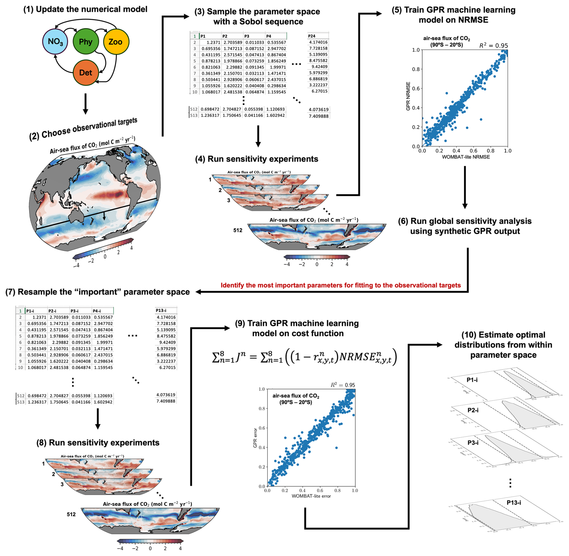
Figure 1 Flow chart representation of the methodology. (1) Any updates to the numerical model, in this case a biogeochemical model, are finalized. Because the model has been altered, it requires optimization. (2) The target observations are chosen against which the model performance will be assessed and, eventually, optimized. (3) Sobol sequencing of the full parameter space selects 512 unique parameter sets from a priori ranges of the uncertain parameters. In this case, we chose 24 uncertain parameters. (4) The 512 unique parameter sets are used to run the numerical model forward to obtain 512 “simulated” solutions for each of the target observations. (5) Using a metric of model performance, in this case the normalized root mean square error (NRMSE), we train a surrogate machine learning model based on Gaussian process regression (GPR) to synthetically reproduce the model performance (NRMSE) given a parameter set as input. (6) With the GPR model we create thousands of synthetic model simulations to conduct a global Sobol sensitivity analysis. This tells us what the most important parameters are for model performance against our observational targets. (7) We resample the parameter space using only the most important parameters and (8) run a new set of simulations with these unique parameter sets. (9) The GPR model is then trained to reproduce the global cost function (denoted “error” above), which accounts for the performance of the model across all observational targets, given a unique parameter set as input. (10) Thousands of synthetic cost function results, estimated by the GPR model, are used to perform Bayesian optimization that solves for the optimal posterior distributions of the important parameters from within the a priori ranges.

2 Methods

2.1 Optimization summary

We have updated an ocean-biogeochemical model called WOMBAT-lite (Fig. 2). These updates (detailed below) necessitated a thorough sensitivity analysis and optimization to a chosen set of observations. We performed Sobol sensitivity analysis (Sobol', 2001), which gave an understanding of which parameters were most important to the model outcomes, followed by Bayesian optimization to fine-tune parameter values and improve model accuracy. However, both Sobol sensitivity analysis and Bayesian optimization require many thousands of samples to be reliable. To overcome this challenge, we employed a machine learning model based on Gaussian process regression to act as a surrogate of WOMBAT-lite. This computationally inexpensive surrogate was trained on hundreds of real simulations with WOMBAT-lite, predicted global univariate statistics of model error, and was able to produce large samples of synthetic results that enabled sensitivity analysis and optimization (Fig. 1).

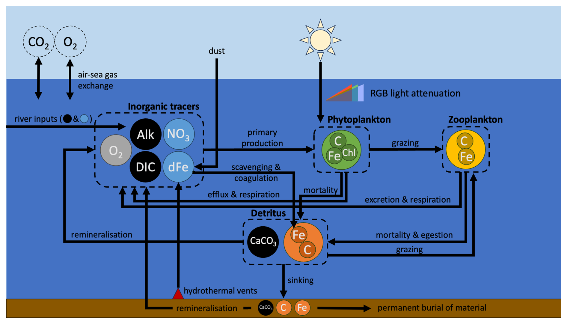
Figure 2 Schematic representation of WOMBAT-lite. Tracers and biomass pools are represented by circles of different colors. Black tracers represent the carbon system; blue are inorganic nutrients. Inner circles of C, Chl and Fe within each biomass pool represent the units of carbon, chlorophyll and iron that are explicitly tracked. Major components are grouped within the dashed outlines. Although dissolved inorganic carbon (DIC), alkalinity (Alk) and oxygen (O₂) are connected to primary production, they are only affected by it and do not limit primary production of phytoplankton. In contrast, both nitrate (NO₃) and dissolved iron (dFe) are biogeochemical tracers whose availability both controls and is affected by phytoplankton growth. Dust and hydrothermal iron input dFe, while rivers input DIC, Alk, NO₃ and dFe. Atmospheric concentrations of carbon dioxide (CO₂) and O₂ are not explicitly tracked by the ocean model (dashed circles).

2.2 Model development summary

Although “lite”, the version of WOMBAT developed for this study is more complex than the previous WOMBAT. Updates include an implicit representation of the packaging effect of cell size, which explicitly controls light attenuation through the water column; explicit photoacclimation of phytoplankton; a dynamic co-limitation of iron and light, whereby phytoplankton require increases in their iron quotas as they photoacclimate (i.e., increase their chlorophyll quotas) under low-light conditions; spatial variations in nutrient affinities of phytoplankton for nitrogen and iron; expanded iron cycling, with additional sinks due to scavenging onto detrital particles, colloidal coagulation and nanoparticle precipitation; riverine sources offset by permanent burial in sediments; a spatially varying sinking rate of detritus that increases with an implicit estimate of mean community cell size and also with depth; simplistic sedimentary denitrification and nitrogen fixation routines; and dampened temperature dependence of zooplankton grazing. WOMBAT-lite (Fig. 2) considers 13 tracers: two nutrients, being nitrate (NO₃) and dissolved iron (dFe); the carbon system (dissolved inorganic carbon (DIC), alkalinity (Alk), calcium carbonate (CaCO₃)); oxygen (O₂); the biomass pools of one phytoplankton (B_p), one zooplankton (B_z) and one sinking detrital (B_d) functional type, prognostic chlorophyll ($B_{\mathrm{p}}^{\mathrm{Chl}}$); and biogenic iron in phytoplankton ($B_{\mathrm{p}}^{\mathrm{Fe}}$), zooplankton ($B_{\mathrm{z}}^{\mathrm{Fe}}$) and sinking detritus ($B_{\mathrm{d}}^{\mathrm{Fe}}$). In WOMBAT-lite, photosynthetically active radiation (PAR) is split into three wavelength bands associated with blue, green and red light, and each of these bands attenuates differently through the water column. The explicit chlorophyll content of phytoplankton allows for photoacclimation and the formation of deep chlorophyll maxima. The attenuation of blue, green and red light is affected by chlorophyll concentrations, and we implicitly account for the “packaging effect” by assuming a positive relationship between chlorophyll concentration and community mean cell size, where larger cells have less effect on light absorption. Phytoplankton limitation by nutrients is affected by an implicit positive relationship between cell size and cell density, where larger cells have less affinity for nutrients. Limitation by iron is modeled via variable quotas, allowing for luxury uptake under dFe-rich conditions and the export of Fe-rich detritus. Phytoplankton increase their iron requirements as their intracellular quota of chlorophyll increases, generating a co-limitation of light and iron on growth. Cycling of dFe now explicitly considers free, ligand-bound and colloidal iron and is lost via nanoparticle formation, scavenging and colloidal coagulation. Zooplankton grazing is via a type III disk formulation that substantially dampens the temperature effect on grazing activity, aligning with rapid consumption rates in polar and tropical waters alike. The sinking of detritus is spatiotemporally variable and is dependent on phytoplankton biomass, emulating community shifts in mean cell size and bloom conditions, and depth, emulating a power law rather than an exponential decay associated with acceleration due to packaging with increasing pressure. A fraction of the detritus (and CaCO₃) reaching the sediment is now permanently buried. In addition, WOMBAT-lite considers inputs of NO₃, DIC and Alk from rivers, simplistic sedimentary denitrification and nitrogen fixation routines, as well as the flux of dFe from hydrothermal vents. All biogeochemical cycles in WOMBAT-lite are therefore open, and their inventories can change. The basic unit of biomass is carbon with a fixed $\mathrm{C}:\mathrm{N}:{\mathrm{O}}_{\mathrm{2}}$ of $\mathrm{122}:\mathrm{16}:-\mathrm{172}$. A full description of WOMBAT-lite is in Appendix A.

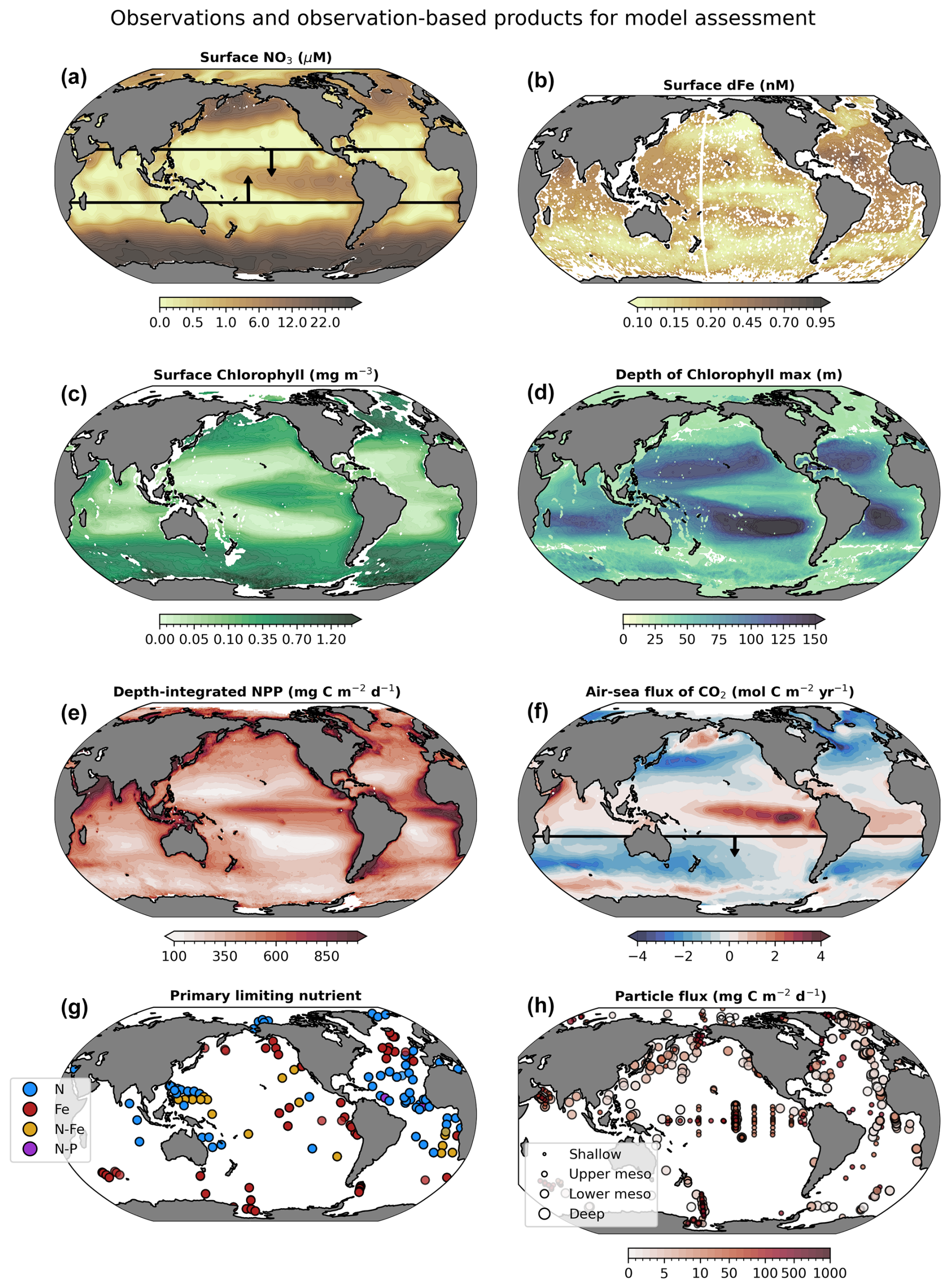
Figure 3 Observation-based target fields used for assessment (sensitivity analysis and optimization) of WOMBAT-lite. Annual means are shown here for illustration purposes, but monthly resolution was used for all products except the Primary Limiting Nutrient dataset (Browning and Moore, 2023). Boxes in maps of surface nitrate (NO₃) and the air–sea flux of carbon dioxide (CO₂) encapsulate the specific regions of focus when assessing model performance and optimization, being between 20° S and 20° N for surface NO₃ and south of 20° S for air–sea CO₂ fluxes. CO₂ fluxes out of the ocean are positive.

2.3 Model experiments and evaluation

2.3.1 Observational target fields for assessment

We use eight observational products/databases to assess the performance of WOMBAT-lite (Fig. 3) including the gridded, global products of surface NO₃ (Garcia et al., 2024a) and dFe (Huang et al., 2022). While nutrient distributions are useful, they have limited power by themselves for assessing biogeochemical models, since similar distributions of nutrients can be achieved for different rates of phytoplankton growth and recycling (Fennel et al., 2022). Remotely sensed chlorophyll is an important constraint that can be considered a proxy for the total stock of phytoplankton biomass and features heavily in biogeochemical model evaluation (Fennel et al., 2022). We use the Copernicus three-dimensional chlorophyll a product that combines remotely sensed, hydrographic and BGC-Argo measurements of fluorescence to generate a depth-resolved climatology of chlorophyll (Sauzède et al., 2015). The extension of chlorophyll to depth allows for an assessment of patterns in the vertical, including spatiotemporal variations in the position of the deep chlorophyll maximum, which we assess in addition to surface chlorophyll concentrations. Other important observations include a gridded and global product of air–sea CO₂ fluxes for the year 1985 (Chau et al., 2022), the earliest year available, and vertically integrated net primary production (Westberry et al., 2008). We opt for CO₂ fluxes rather than pCO₂ to also account for any error in the wind-speed-dependent gas exchange formulation, which we do not update or optimize at this stage. Because the carbon-based productivity model (CbPM; Westberry et al., 2008) is based on backscatter and explicitly accounts for growth rates separate from biomass, its patterns are more orthogonal to chlorophyll than the Vertically Generalized Production Model (VGPM; Behrenfeld and Falkowski, 1997) and so offers greater potential as an independent constraint on model performance (Westberry et al., 2023). Net primary production (NPP) built from the CbPM products should therefore provide more independent constraints on model assessment than an NPP product built from chlorophyll concentrations. In addition to these gridded products, we also use a database of the primary limiting nutrient for phytoplankton growth (Browning and Moore, 2023) and sediment trap records of the sinking flux of detrital particles through the ocean interior (Mouw et al., 2016). For the primary limiting nutrient dataset, we only consider nitrogen and iron as limiting (excluding phosphorus) and ascribe nitrogen limitation, iron-nitrogen co-limitation and iron limitation as equal to 1.0, 1.5 and 2.0, respectively. This is compared directly to the degree of limitation by the model, which varies continuously from strong nitrogen limitation to strong iron limitation (1.0 to 2.0). Although the model does not include co-limitation as a process, simulated values between 1.0 and 2.0 can represent seasonal variations between nitrogen and iron limitation over an annual timescale.

While we recognize that these datasets are themselves subject to uncertainty, their combination allows for a powerful model assessment. Furthermore, our assessment focuses on the reproduction of large-scale, seasonal patterns. It is also worth noting that having too many target fields compounds the difficulty associated with parameter optimization, while having too few risks poor performance in unconsidered targets. Target fields must therefore be chosen carefully. All gridded datasets as well as the particle flux database are resolved on a global 1° by 1° grid and on a monthly temporal resolution, while the primary limiting nutrient for phytoplankton, due to data paucity, is represented annually (unchanging in time).

2.3.2 Sensitivity experiments for evaluation and surrogate model training

Our first goal was to understand which parameters in WOMBAT-lite were most important for model performance. We undertook 512 simulations that each sampled randomly from predefined ranges of 24 key parameters related to the ecosystem component of the model (Table 1, Fig. 1) using a quasi-Monte Carlo Sobol sequence (see Sect. 2.4). A total of 512 experiments were selected because this was enough for training the surrogate machine learning model to an acceptable standard (Fig. S1 in the Supplement). Each experiment carried a unique biogeochemical parameter set that altered the biogeochemical behavior, but all experiments had identical physical conditions and initial conditions. Physical fields were initialized from a previous spin-up with the same ocean model (Kiss et al., 2020) forced by JRA55-do (Tsujino et al., 2018). We used a repeat “normal” year forcing of the JRA55-do to avoid inter-annual variability and extremes in climate modes (Stewart et al., 2020). Atmospheric CO₂ was maintained at 315.2 ppm (i.e., levels at calendar year 1958). NO₃, dFe, O₂, DIC and Alk fields were initialized from globally gridded datasets for the month of December (Garcia et al., 2024a, b; Huang et al., 2022; Lauvset et al., 2016). Concentrations of phytoplankton, zooplankton, detritus and CaCO₃ were initialized at globally homogenous values of 0.1 mmol C m⁻³. Fe:C ratios of phytoplankton, zooplankton and detritus were initialized at 7 µmol mol⁻¹. Chlorophyll was initialized at 0.004 mg mg⁻¹ of phytoplankton carbon biomass.

Table 1 Key ecosystem parameters for WOMBAT-lite and their predefined ranges for ocean-only experiments. Parameter values for other configurations, including for the Earth system model (ACCESS-ESM1.6), are available at https://github.com/ACCESS-NRI (last access: 1 September 2025).

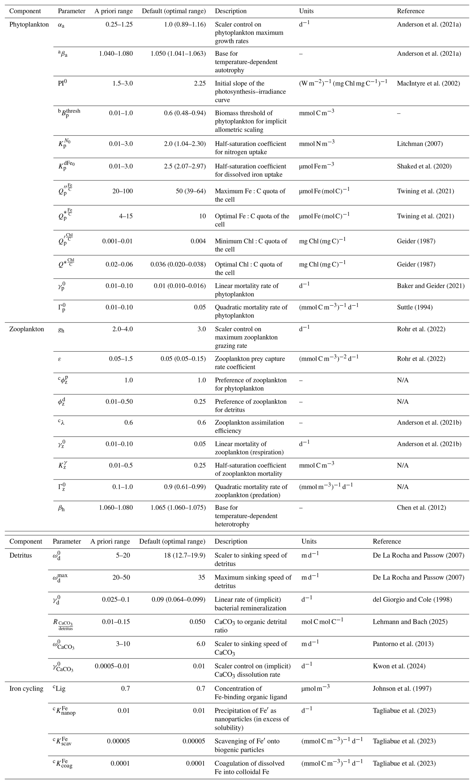
^a Parameter variations not included in initial sensitivity experiments for sensitivity analysis (steps 3–6 in Fig. 1). Only in optimization (steps 7–10 in Fig. 1).
^b Parameter range was set equal to 0.01 to 0.1 in the initial sensitivity experiments for sensitivity analysis (steps 3–6 in Fig. 1).
^c Parameter space not explored.

We chose to run the experiments for only 10 years, making a total of 5120 model years, and at a nominal horizontal resolution of 1°. This short timescale was sufficient to assess the skill of the biogeochemical model, at least regarding its ecosystem component. Marine phytoplankton contribute half of all primary production in the Earth system (Field, 1998) but represent less than 1 % of photosynthetic biomass (Friedlingstein et al., 2023; Le Quéré et al., 2005), meaning that they turn over quickly. Changes to key parameters within the ecosystem component therefore result in a rapid realization of different patterns in biological states (e.g., chlorophyll and net primary production, among others). Our analyses and optimization thus focus on the ecosystem component and the upper ocean using 10-year model runs. We do acknowledge that longer-term, low-frequency modes of variation exist in biogeochemical models, and to partially address this we completed 100-year simulations with 20 optimal parameter sets. We note that longer integrations risk the compounding of physical and biogeochemical model errors as the physical state drifts further from the observations, even when applying a repeat climatological atmospheric forcing. Our optimization therefore does not counteract the potential for long-term drift but does provide some guardrails against rapid deviations from the initial state with respect to dissolved nutrient and carbon fields. Optimization of the biogeochemistry under these conditions can cause over-tuning of the biogeochemical parameter set that compensates for physical errors (e.g., Singh et al., 2025). However, by assessing the cost function after 100 years and selecting the best performing of the optimal experiments we likely select for a parameter set with minimal long-term drift.

2.3.3 Measures of performance

Output from the final year of the experiments (year 10) was compared directly to the target datasets (Fig. 3). Univariate measures of performance were calculated, including the correlation coefficient (Pearson's), root mean square error, global mean bias and the normalized standard deviation (Stow et al., 2009). These were calculated across all grid cells and time points. For surface NO₃ concentrations, we only calculated these statistics between 20° S and 20° N to focus on achieving a realistic transition of higher concentrations to lower concentrations from the equatorial to subtropical biome. We stress that fidelity in extra-tropical regions was captured independently via the limiting nutrient dataset. Also, surface NO₃ in the equatorial region is highly responsive to changes in the ecosystem component due to warmer temperatures that accelerate metabolism. After only 10 years our simulations diverged most in this region. Additionally, surface NO₃ concentrations were log₁₀ transformed prior to calculating the measures of performance due to a skewed distribution towards very low values. This substantially improved the ability of our optimization approach to select parameters that reproduced the high-NO₃ tongue in the equatorial region (see below). For air–sea fluxes of CO₂, we assessed model performance exclusively in the Southern Ocean south of 20° S. This region was also highly sensitive to the parameterizations of the model, showing positive or negative fluxes depending on our parameter set and aligning with findings that biological activity in this region is of high importance for model skill (Mongwe et al., 2018).

2.4 Details of the sensitivity analysis and model optimization

2.4.1 Global sensitivity analysis

Sensitivity analysis (SA) methods are broadly categorized into local and global approaches. Local SA examines how small perturbations in parameters around certain reference points affect outputs, making it computationally feasible and widely used (Rakovec et al., 2014). However, for models where parameters interact or have non-linear impacts on the outputs, local SA can introduce substantial bias, underestimating parameter importance (Saltelli et al., 2019). The model parameters in this study are anticipated to exhibit complex, non-linear interactions influencing the outputs (Denman, 2003; Fennel et al., 2022; Matear, 1995; Ward et al., 2010), thus justifying the use of global SA to capture these dynamics accurately. One of the most effective global SA methods, Sobol sensitivity analysis, is widely adopted due to its precision in addressing interaction effects, discontinuities and non-linear influences of parameters on model outputs (Baki et al., 2022; Reddy et al., 2024b). Based on the Hoeffding–Sobol decomposition, Sobol SA leverages analysis of variance (ANOVA) to decompose output variance into contributions from individual parameters, interactions between parameter pairs and so on across increasing levels of dimensionality (Saltelli et al., 2010; Sobol', 2001). Sobol sensitivity indices, representing the importance of parameter interactions in the context of total output variance, are then computed by evaluating ratios of these variances. Performing Sobol SA on the WOMBAT-lite outputs requires extensive parameter sampling, a computationally expensive task. To efficiently manage this, we use a surrogate Gaussian process regression (GPR) model (Williams and Rasmussen, 1995, 2006), which is trained on a limited number of runs (sensitivity experiments; Sect. 2.3.2; visualized in Fig. 1). The GPR model, designed for accuracy, provides predictions over a large sample space, allowing SA to be performed without extensive and computationally unfeasible simulations.

The analysis focuses on the target fields detailed in Fig. 3 and Sect. 2.3.1. To generate the 512 sensitivity experiments required to train the surrogate machine learning model, a quasi-Monte Carlo Sobol sequence is applied to generate 512 parameter samples using the Uncertainty Quantification Python Laboratory package (UQ-PyL; Wang et al., 2020). Simulations are then run with these parameter samples, and the relative root mean square error (rRMSE) values are calculated by comparing the model outputs with observational data in space and time. The rRMSE is then normalized (NRMSE) via min–max scaling. A sample size of 512 is selected based on the sample size sensitivity experiments (Fig. S1). Next, GPR models are trained for each observational target using these parameter samples as inputs and the NRMSE as the output. NRMSE was chosen as a metric of performance because of our diversity of target fields, each with different units, which required normalization to ensure that each contributed equally to an assessment of global performance. K-fold cross-validation is used to evaluate the GPR model's accuracy, and we chose 8 folds (K=8) to cleanly divide the 512 experiments and provide a balance between sufficient training (448) and testing data (64) (Reddy et al., 2024a). The data are split into K folds, and the model is trained on K−1 folds, with the left-out fold serving as the test set. This is repeated across all folds, and predictions are aggregated. The GPR model accuracy is assessed through the goodness-of-fit (R²) metric by comparing GPR predictions of NRMSE with WOMBAT-lite NRMSE data, which indicates high accuracy (Fig. S2). Using this validated GPR model, NRMSEs for 53 248 new parameter samples (generated via Sobol sequence) are predicted for each target field (all eight), consistent with methods from previous studies (Baki et al., 2022; Reddy et al., 2024b). Finally, Sobol sensitivity indices are calculated based on these predictions for all eight target fields, offering insight into the relative influence of each parameter on the ability of WOMBAT-lite to reproduce the targets.

2.4.2 Parameter optimization

Following sensitivity analysis, which identified the most important parameters for model performance (NRMSE) of the eight target fields, we performed parameter optimization (Fig. 1). This study uses Gaussian process regression-based Bayesian optimization (G-BO) (Reddy et al., 2024a) to identify the optimal parameter distributions so that WOMBAT-lite can best reproduce the eight target fields simultaneously. The process begins by generating another 512 parameter samples via the same quasi-Monte Carlo (QMC) Sobol sequence design implemented through the UQ-PyL package (Wang et al., 2020). This set of 512 sensitivity experiments is different from those generated during the sensitivity analysis because we now use a reduced set of only the most important parameters, which also provides a denser sampling of the parameter space essential for the G-BO process (Reddy et al., 2024a). These 512 sample parameter sets are used as input to WOMBAT-lite, and the model is run forward for 10 years (see above). A sample size of 512 is selected based on the sample size sensitivity experiments (Fig. S3). Then, the GPR surrogate model, trained on these 512 samples, predicts a normalized cost function for each target field,

$$\begin{array}{}\text{(1)}& J=\left(\mathrm{1}-r_{x,y,t}\right)\cdot {\text{NRSME}}_{x,y,t},\end{array}$$

where J is the cost function for a given target field, ${\text{NRSME}}_{x,y,t}$ is the normalized root mean square error (scaled by the max–min, such that the worst experiment has an NRMSE of one, and the best is zero), and $r_{x,y,t}$ is Pearson's correlation coefficient evaluated across all longitude (subscript x), latitude (subscript y) and time (subscript t) points (time in this case being monthly in resolution). Unlike the sensitivity analysis that measured model performance purely via the NRMSE, this cost function also penalizes poor correlations. Rather than optimize for the parameters that best reproduce each target field in isolation, we chose to optimize to a global cost function

$$\begin{array}{}\text{(2)}& \sum _{\left(n\right)=\mathrm{1}}^{\mathrm{8}}{J}^{\left(n\right)}=\sum _{\left(n\right)=\mathrm{1}}^{\mathrm{8}}\left(\left(\mathrm{1}-r_{x,y,t}^{\left(n\right)}\right){\mathrm{NRMSE}}_{x,y,t}^{\left(n\right)}\right),\end{array}$$

where superscript n is the nth target field. Therefore, we select parameter sets that optimize overall model performance by summing the prediction errors from all eight surrogate GPR models. Using a composite kernel – constant, Matérn and white noise kernels with hyperparameters guided by previous work (Reddy et al., 2024a) – the GPR model accurately predicts the normalized cost function values, confirmed by R² scores >0.8 from K-fold cross-validation (K=8) (Fig. S4). The trained GPR model is then used to estimate the normalized cost function value for optimization purposes. Although expected, we note that the predicted cost functions using the GPR models are not completely orthogonal, with some being well correlated (Fig. S5), indicating that the optimization of parameters towards one target field will affect other target fields.

Bayesian optimization enables iterative learning of optimal model parameters using observational data. Here, we apply uniform priors under the assumption that there is equal probability of the optimal values falling anywhere between what are known lower and upper bounds (Table 1). The priors are normalized from 0 to 1 via max–min scaling, and the normalized cost function value predicted by the GPR model serves as the likelihood function (Reddy et al., 2024a). Since computing marginal likelihood directly is often complex, Markov chain Monte Carlo (MCMC) sampling is employed, which estimates the posterior distribution without explicit calculation of this constant (Issan et al., 2023). Normalization of priors between 0 and 1 ensures more efficient exploration of the high-dimensional parameter space (i.e., better “mixing”) and therefore more reliable convergence, while normalization of the cost functions ensures equal weighting of each target field to the solution. Among MCMC methods, affine invariant ensemble sampling, implemented using the “emcee” Python package (Foreman-Mackey et al., 2013), is selected for its efficient convergence properties. This method uses an ensemble of chains to simplify sampling from anisotropic distributions. Fifty walkers and a stretch move of two are applied, with the first 10 000 steps used as a burn-in phase to ensure convergence, followed by 90 000 additional steps to achieve stable posterior distribution estimates (Foreman-Mackey et al., 2013; Goodman and Weare, 2010). This substantial burn-in phase converts our uniform priors into distributions that look more like the posterior (Foreman-Mackey et al., 2013). In total, 90 000 steps for each of the 50 walkers means a total of 4 500 000 random walks, and with a mean autocorrelation time of 690 steps, we achieve 6500 independent samples of the posterior. This number of samples, made possible by the efficiency of the surrogate GPR model, is more than sufficient for convergence. Convergence was also evident by a mean acceptance fraction of 0.22 (Foreman-Mackey et al., 2013), a Gelman–Rubin statistic of between 1.005 and 1.009 for each parameter, and visual assessment of the chains (Fig. S6).

3 Results

3.1 Performance

The 512 sensitivity experiments, each with a unique parameter set (Table 1), produced 512 unique realizations of biogeochemical and ecosystem dynamics. We compared year 10 of the experiments at all grid cells and at monthly temporal resolution with the target datasets (i.e., the observations). The skill of these simulations ranged widely (Fig. 4, Table 2). Global surface chlorophyll showed the greatest variation, ranging in correlations from −0.45 to 0.8, followed by the primary limiting nutrient of phytoplankton growth (−0.29 to 0.82) and the depth of the chlorophyll maximum (−0.25 to 0.69). Most experiments underestimated the variability in surface chlorophyll, and many produced surface chlorophyll concentrations that were low compared with the observation-based product. Unlike surface chlorophyll, there was too much variation in the depth of the chlorophyll maximum, and many experiments had chlorophyll maxima that were positioned too deep (i.e., positive bias).

For the air–sea flux of CO₂ in the Southern Ocean (20–90° S) and the depth-integrated rate of net primary production, our simulations showed a narrow range of correlations between 0 and 0.5. The narrower range potentially reflects the identical physical state across our experiments, which strongly influences air–sea gas exchange and nutrient delivery to the surface. For net primary production, the weaker correlations might reflect significant errors in the observation-based products themselves (Westberry et al., 2023) that limit the potential for agreement. Like chlorophyll, net primary production showed a negative bias in many experiments and a chronic inability to capture the observed magnitude of variations. The same general underestimation of values and variability was the case for the sinking flux of detritus. No experiment was able to reproduce the observed spatiotemporal variations in sinking detrital flux, although this is perhaps expected given that this dataset captures higher-frequency variations in particle flux that are lost in a coarse-resolution model.

For surface dFe, the experiments produced correlations ranging from −0.13 to 0.52, and thus the best-performing experiments compared well with other biogeochemical models (Huang et al., 2022). Finally, the primary limiting nutrient of phytoplankton growth (i.e., nitrogen or iron) showed biases and correlations ranging from negative to positive, indicating that some were too nitrogen-limited, some were too iron-limited, and some performed well.

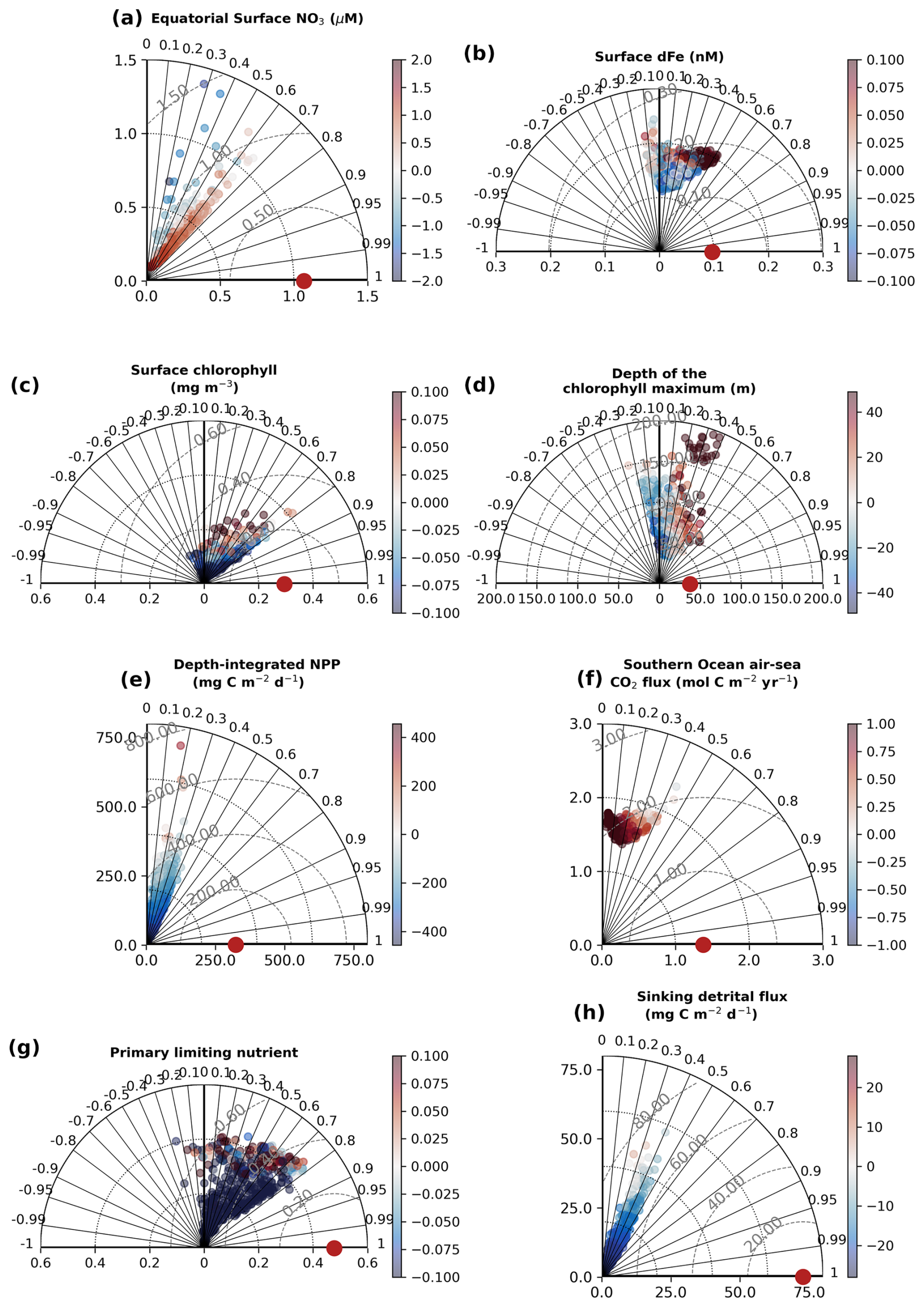
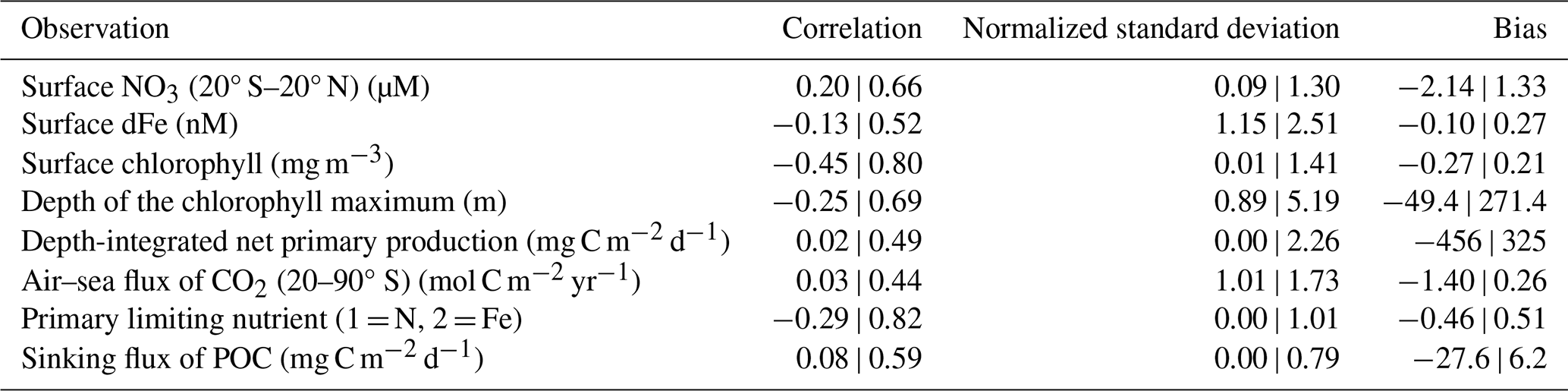
Figure 4 Performance of the 512 sensitivity experiments with WOMBAT-lite against the 8 key observational targets. Taylor diagrams (Taylor, 2001) represent the agreement between a dataset and the target (red dot) by visualizing the dataset in terms of its correlation (radii), normalized standard deviation (x and y axes) and the centered root mean square error (dashed gray contours). We also color each experiment by its global mean bias. Positive bias in the Southern Ocean air–sea flux of CO₂ signifies too much outgassing or not enough ingassing. These statistics were computed on the global 1° by 1° grid at monthly resolution, except the Primary Limiting Nutrient dataset, which was computed as an annual mean.

Table 2 Performance ranges of experiments for key observations. Minimum and maximum values of correlations, normalized standard deviations and bias across all 512 sensitivity experiments. Surface NO₃ was log₁₀ transformed. NO₃: nitrate; dFe: dissolved iron; CO₂: carbon dioxide; POC: particulate organic carbon.

3.2 Global sensitivity analysis

Global sensitivity analysis with our first set of 512 experiments and supplemented by the surrogate machine learning model revealed that the overall performance of WOMBAT-lite was sensitive to 11 of the 24 parameters tested, based on an arbitrary threshold of a 5 % contribution to variation (Fig. 5). These were the scaler on the maximum growth (α_a) and linear mortality rates of phytoplankton (${\mathit{\gamma }}_{\mathrm{p}}^{\mathrm{0}}$), the half-saturation coefficients for phytoplankton uptake of dFe ($K_{\mathrm{p}}^{\mathrm{dFe}}$) and NO₃ ($K_{\mathrm{p}}^{\mathrm{N}}$), the maximum quota of iron ($Q_{\mathrm{p}}^{\prime \prime \frac{\mathrm{Fe}}{\mathrm{C}}}$) and optimal quota of chlorophyll ($Q_{\mathrm{p}}^{\ast \frac{\mathrm{Chl}}{\mathrm{C}}}$), the prey capture rate coefficient of zooplankton (ε) and their quadratic mortality rate (${\mathrm{\Gamma }}_{\mathrm{z}}^{\mathrm{0}}$), the sinking (${\mathit{\omega }}_{\mathrm{d}}^{\mathrm{0}}$) and remineralization (${\mathit{\gamma }}_{\mathrm{d}}^{\mathrm{0}}$) rate of detritus, and the temperature sensitivity of heterotrophy (β_h). The initial slope of the photosynthesis–irradiance curve (PI⁰) was not included because it fell just below the 5 % threshold (shown rounded up in Fig. 5b) in its higher-order effects. For each of the eight target fields, typically only a few of these key parameters were influential. We step through these parameters here.

All target fields were highly sensitive to the phytoplankton maximum growth rates (α_a) and their linear mortality (${\mathit{\gamma }}_{\mathrm{p}}^{\mathrm{0}}$) (Fig. 5). Of these, only the depth of the chlorophyll maximum and surface dFe concentrations were sensitive to α_a and ${\mathit{\gamma }}_{\mathrm{p}}^{\mathrm{0}}$ via interactive effects with each other or other variables (i.e., higher-order interactive effects). All other target fields were directly affected by these parameters, making α_a and ${\mathit{\gamma }}_{\mathrm{p}}^{\mathrm{0}}$ master parameters with largely predictable effects for controlling the performance and output of WOMBAT-lite. For example, while the air–sea flux of CO₂ in the Southern Ocean (south of 20° S) was sensitive to several parameters, the model's ability to reproduce the observations was primarily controlled by the ability of phytoplankton to accumulate biomass rapidly in the spring and summer. If ${\mathit{\gamma }}_{\mathrm{p}}^{\mathrm{0}}$ was too high, then too much biomass was lost over the winter, causing a lag in the spring bloom. If α_a was too low, then the bloom would be too weak. The link between CO₂ ingassing in the summer and the phytoplankton bloom also meant that the prey capture rate coefficient of zooplankton (ε), the half-saturation coefficient for dFe uptake by phytoplankton ($K_{\mathrm{p}}^{\mathrm{dFe}}$) and the sinking rate of detritus (${\mathit{\omega }}_{\mathrm{d}}^{\mathrm{0}}$) were also important controls on CO₂ fluxes in the Southern Ocean.

Surface NO₃ concentrations in the tropics (20° S–20° N), depth-integrated net primary production and the sinking flux of detritus were all affected by similar parameters. After α_a and ${\mathit{\gamma }}_{\mathrm{p}}^{\mathrm{0}}$, the parameters of influence were the sinking and remineralization rates of detritus (${\mathit{\omega }}_{\mathrm{d}}^{\mathrm{0}}$ and ${\mathit{\gamma }}_{\mathrm{d}}^{\mathrm{0}}$). Elevated sinking rates and decelerated remineralization both deepen the nitracline by stripping more NO₃ out of the upper ocean and shrinking the large tongue of high-NO₃ water that spreads west across the equatorial Pacific. Surface NO₃ in the equatorial band was also marginally affected by the temperature sensitivity of heterotrophy (β_h), which amplifies remineralization rates (set also by ${\mathit{\gamma }}_{\mathrm{d}}^{\mathrm{0}}$) in warmer waters and so can increase substantially how much detritus is returned to inorganic nutrients.

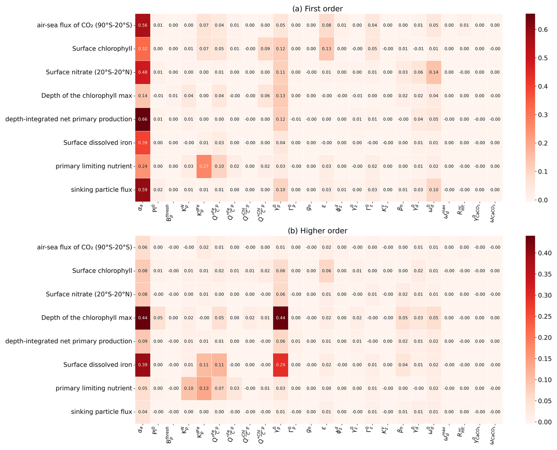
Figure 5 Sensitivity of WOMBAT-lite performance to variations in the parameters listed in Table 1. Performance is measured by the root mean square error (RMSE), which is normalized here by the full range (max–min scaling). First-order indices are a direct individual effect of a parameter on the target field, while higher-order indices indicate that interaction effects with other parameters are important. First-order indices sum to at most one for a given target field, while first-order + higher-order indices sum to at least one. If there are no interaction effects, then higher-order effects are nil. Darker colors indicate a greater sensitivity of a target field to the parameter in question. In (a) we show first-order sensitivities and in (b) the higher-order sensitivities, otherwise referred to as an interaction effect, where the effect on the target is dependent on the variations in other parameters. Note that the parameter β_a was not included at this stage but only later during the optimization process (steps 7–10 in Fig. 1).

Two key parameters controlling the model's ability to reproduce surface dFe (after α_a and ${\mathit{\gamma }}_{\mathrm{p}}^{\mathrm{0}}$) and the primary limiting nutrient dataset were the half-saturation coefficient for dFe uptake ($K_{\mathrm{p}}^{\mathrm{dFe}}$) and the maximum Fe:C quota of phytoplankton ($Q_{\mathrm{p}}^{\prime \prime \frac{\mathrm{Fe}}{\mathrm{C}}}$). Variations in these parameters had strong interactive effects. Elevating iron quotas increased the ability of phytoplankton to take excess dFe into their biomass, reduced surface dFe concentrations and strengthened iron limitation as more Fe-rich biomass was exported as sinking detritus. However, if we also increased the half-saturation coefficient of dFe uptake, this slowed phytoplankton luxury uptake of dFe and made them less likely to achieve high intra-cellular Fe:C quotas. As such, setting higher Fe:C quotas had little effect on surface dFe concentrations when $K_{\mathrm{p}}^{\mathrm{dFe}}$ was high. On the other hand, setting high Fe:C quotas can have a substantial effect on dFe concentrations when $K_{\mathrm{p}}^{\mathrm{dFe}}$ is low. For the primary limiting nutrient dataset, however, we found that increasing both Fe:C quotas and $K_{\mathrm{p}}^{\mathrm{dFe}}$ elevated dFe limitation regardless of what happened to the dFe concentrations.

Performance in surface chlorophyll was the most interdependent metric, meaning that many parameters were influential. In addition to the master parameters of α_a and ${\mathit{\gamma }}_{\mathrm{p}}^{\mathrm{0}}$, surface chlorophyll was affected by the maximum Fe:C quota ($Q_{\mathrm{p}}^{\prime \prime \frac{\mathrm{Fe}}{\mathrm{C}}}$), the half-saturation of dFe uptake ($K_{\mathrm{p}}^{\mathrm{dFe}}$), the maximum quota of chlorophyll to carbon in phytoplankton ($Q_{\mathrm{p}}^{\prime \prime \frac{\mathrm{Chl}}{\mathrm{C}}}$), the prey capture rate coefficient of zooplankton (ε) and marginally the quadratic mortality coefficient of zooplankton (${\mathrm{\Gamma }}_{\mathrm{z}}^{\mathrm{0}}$). Thus, 7 of the 11 important parameters were influential. The fact that many parameters were crucial for determining the performance of surface chlorophyll reflects that a delicate balance between phytoplankton growth and mortality must be struck to reproduce overall biomass.

Finally, the depth of the chlorophyll maximum was overwhelmingly influenced by α_a and ${\mathit{\gamma }}_{\mathrm{p}}^{\mathrm{0}}$, with weaker influences from the half-saturation coefficient for nitrogen uptake ($K_{\mathrm{p}}^{\mathrm{N}}$), cell quotas of iron and chlorophyll ($Q_{\mathrm{p}}^{\prime \prime \frac{\mathrm{Fe}}{\mathrm{C}}}$ and $Q_{\mathrm{p}}^{\prime \prime \frac{\mathrm{Chl}}{\mathrm{C}}}$), and parameters related to the sinking and remineralization of detritus (β_h, ${\mathit{\omega }}_{\mathrm{d}}^{\mathrm{0}}$ and ${\mathit{\gamma }}_{\mathrm{d}}^{\mathrm{0}}$). All these parameters affected the depth of the nitracline in direct and indirect ways, to which the depth of the chlorophyll maximum was strongly linked. Increasing α_a while simultaneously decreasing ${\mathit{\gamma }}_{\mathrm{p}}^{\mathrm{0}}$, for example, would cause an accelerated deepening of the nitracline since phytoplankton consume more nutrients but can also survive for longer under light limitation at depth.

3.3 Parameter optimization

Our optimization procedure involved another 512 experiments that varied 13 parameters: the 11 parameters identified in the sensitivity analysis plus 2 additional parameters that were missed by our sensitivity analysis. The additional two parameters included wider variations in the biomass threshold of phytoplankton for allometric scaling ($B_{\mathrm{p}}^{\mathrm{thresh}}$) from 0.01 to 1.0 (previously this had been varied from 0.01 to 0.1), as well as variations in the base scaler of temperature-dependent autotrophy (β_a), which was previously held constant during the sensitivity experiments at a value of 1.066 (Q₁₀=1.89), following Eppley (1972) but has nonetheless been shown to vary between phytoplankton types (Anderson et al., 2021a). We took the opportunity during the optimization to vary these parameters. In our optimization step, we explored a range of 1.040 to 1.080 (Q₁₀ from 1.48 to 2.16) in β_a motivated by the results of Anderson et al. (2021a). All remaining, insensitive parameters were held at their default values (Table 1). Thus, we explored variations in 13 parameters (11 parameters from the sensitivity analysis and 2 additional parameters) and sought their optimal values for best reproducing the 8 target fields (Fig. 3) by minimizing the global cost function (Eq. 2). The 512 experiments were used to train the surrogate GPR model to reproduce the global cost function, and this training was then used to synthetically estimate the optimal parameter values.

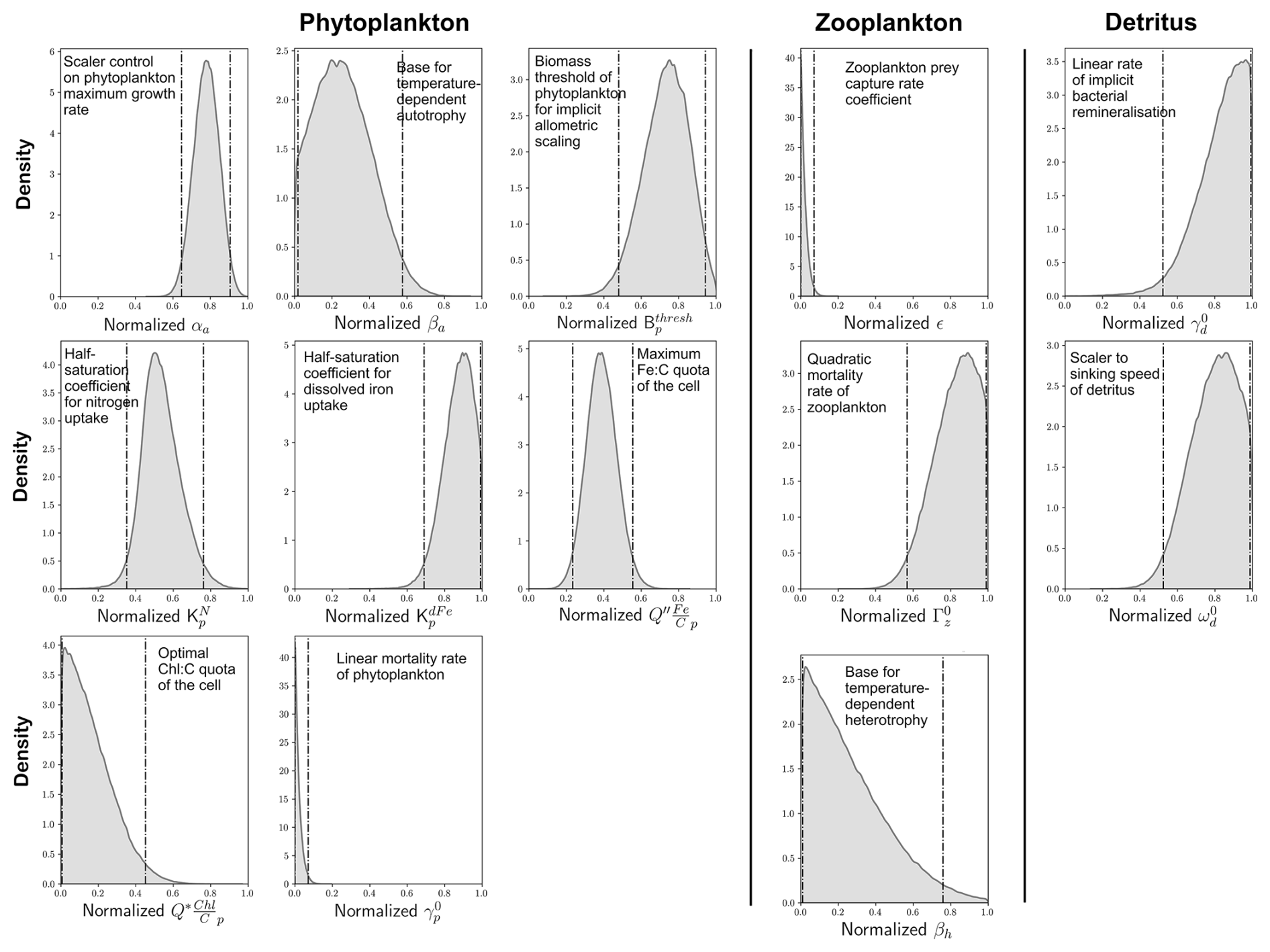
Figure 6 Optimal probability density functions of 13 important parameters. Optimization involved minimizing the global (summed) cost function (Eq. 2) of model performance across the eight target variables shown in Fig. 3. We show normalized distributions of each parameter here and refer the reader to the ranges (a priori and optimal) shown in Table 1 for their actual values. Vertical dashed lines denote 95 % confidence intervals. Parameters are organized according to whether they control phytoplankton, zooplankton or detritus.

We identified posterior distributions of each of the 13 parameters from which optimal values could be chosen (Fig. 6). Optimal values for each of these parameters and their 95 % confidence interval range are detailed in Table 1. For most of the parameters, the probability distributions showed peaks away from the edges of the predefined ranges, suggesting that our a priori ranges were sufficiently wide to capture the optimal values. For the scaler on maximum growth rates of phytoplankton (α_a), for instance, the model predicted optimal values with 95 % confidence between 0.89 and 1.16 d⁻¹, a range that sits within our a priori range of 0.25 to 1.25 d⁻¹ (Table 1) and suggests that the rapid accumulation of biomass during the growth season is crucial for model performance. We also note that the model predicted optimal values that often aligned well with ecological theory. Higher values of $K_{\mathrm{p}}^{\mathrm{dFe}}$ over $K_{\mathrm{p}}^{\mathrm{N}}$ (half-saturation coefficients for uptake) reflect the lesser bioavailability of dFe relative to that of inorganic nitrogen due to its complexation with organics (Shaked et al., 2020; Tagliabue et al., 2017). Fidelity to observations was also better when the temperature sensitivity of autotrophy (β_a) was much lower than the temperature sensitivity of heterotrophy (β_h), consistent with ecological theory on metabolism (Brown et al., 2004) and experimental data (Chen et al., 2012).

Optimal values for two parameters were predicted at the lower edge of their range (Fig. 6). These were the linear mortality rate of phytoplankton at 0 °C (${\mathit{\gamma }}_{\mathrm{p}}^{\mathrm{0}}$) and the prey capture rate coefficient of zooplankton (ε), for which the optimal values were predicted at 0.01 d⁻¹ and 0.05 (mmol C m⁻³)⁻² d⁻¹, respectively (Table 1). Given that ${\mathit{\gamma }}_{\mathrm{p}}^{\mathrm{0}}$ was strongly influential to the ability of WOMBAT-lite to reproduce all eight of our target fields, it is likely that lower values of this parameter than explored herein would produce a better fit to the observations. Rates of mortality considerably lower (<0.001 d⁻¹) than the lowest value in our a priori range (0.01 d⁻¹) were observed in phytoplankton cultures grown within their thermal niche (Baker and Geider, 2021). However, mortalities also increase severely at higher temperatures (Baker and Geider, 2021), and our choice of higher values in our a priori range was motivated by an attempt to account for the small proportion of phytoplankton taxa placed above their thermal niche or affected by other sources of environmental stress at any given time. The fact that our optimization always chose the lowest values (near 0.01 d⁻¹) perhaps suggests that, at least with our simple model, the proportion of the community that is stressed is lower than initially assumed. Similarly, optimal values of ε, the zooplankton prey capture rate coefficient, tended towards the lowest of our predefined range. This parameter was a strong control on the model's ability to reproduce the observed surface chlorophyll and the summer uptake of CO₂ in the Southern Ocean (Fig. 5). Values less than 0.05 (mmol C m³)⁻² d⁻¹ suggest grazing pressure more in line with a zooplankton community with a large representation of mesozooplankton (Rohr et al., 2022). This type of community is typical for eutrophic and high-latitude regions but may not be representative of zooplankton grazers in the oligotrophic gyres (Rohr et al., 2024). Importantly, the lower grazing pressure associated with this type of zooplankton community would allow phytoplankton growth during the spring to outpace zooplankton grazing for longer, which we note again was important for achieving summer CO₂ uptake in the Southern Ocean. While we cannot say whether an expanded range would have selected for even lower values, we note that a value near 0.05 (mmol C m³)⁻² d⁻¹ sits at the global median of empirical estimates across a large range of zooplankton taxa (Rohr et al., 2022).

3.4 Outcomes

3.4.1 Finding the optimal parameter set

After our optimization, we chose 20 randomly sampled parameter sets from the optimal posterior distributions shown in Fig. 6 and ran WOMBAT-lite forward for 10 years from initial conditions. These optimal versions of WOMBAT-lite show good fidelity to the target fields, with all registering good performances in terms of the global cost function that were as good as or better than the best of the 512 sensitivity experiments for the majority of the target fields (compare yellow and gray bars in Figs. 7, S6). Continuing to run the model forward for 100 years post-initialization showed some degradation in the performance (red bars in Fig. 7). This is expected, since our optimization procedure was trained on model output only 10 years post-initialization due to computational constraints. Model outcomes drift further away from the target fields with longer integrations. Lower-frequency variability and trends are thus missed by the optimization but are nonetheless present in the biogeochemical model, and these play out as the model is integrated forward for longer. After 100 years, we chose our best performing parameter set, detailed in Table 1 (red star in Fig. 7). This experiment showed good performance across all observational metrics in its 100th year, and we hereafter show output from this experiment.

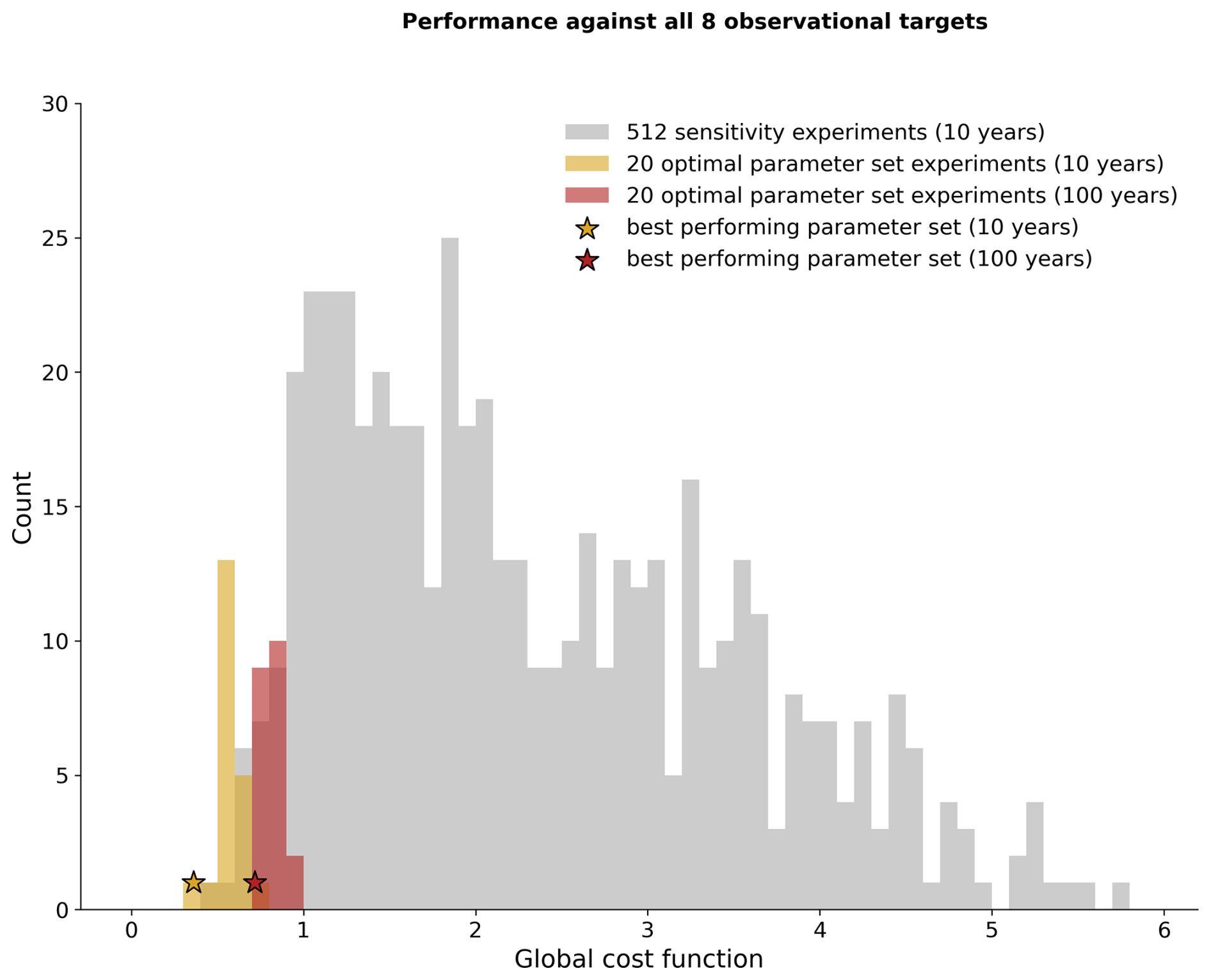
Figure 7 Overall performance of WOMBAT-lite in terms of the global cost function (summed across all target variables; Eq. 2). We show all 512 sensitivity experiments (gray bars), the 20 optimal experiments that selected parameter values randomly from the optimal probability density functions (Fig. 6) after 10 years (gold bars) and 100 years (red bars), and the performance of the optimal parameter set after 10 years (gold star) and 100 years (red star).

3.4.2 Performance improvements

A key challenge in model development is that the addition of new processes can degrade performance if the new processes are implemented poorly and/or if these processes have complex interactive effects once introduced. Our sensitivity analysis and optimization procedure provided a means to constrain both the effects and values of the WOMBAT-lite parameter set so that any advances in functionality are accompanied by an improvement in performance. We take the opportunity to compare the optimized WOMBAT-lite with a prior version that did not undergo this same optimization process but was nonetheless tuned manually (Appendix A1) and run under the same conditions and without the functional improvements described in Appendix A2. The optimized WOMBAT-lite shows a better tropical distribution of surface NO₃ (Fig. 8a–c); lower concentrations of dFe at the surface (Fig. 8d–f); and, consequently, the appearance of iron-limited regimes for phytoplankton growth in the Southern Ocean, subarctic North Pacific and Atlantic, and eastern equatorial Pacific as well as the upwelling centers of the Benguela, Arabian and Canary current systems (Fig. 8s–u). Note that the surface dFe distribution shown in Fig. 8 is of the annual average, which includes higher concentrations caused by winter mixing (Tagliabue et al., 2014b), whereas much of the observations will have been taken during the polar summer, when dFe concentrations are drawn down by biology. WOMBAT-lite also shows a 50 % increase in globally integrated net primary production (from 18.5 to 27.9 Pg C yr⁻¹) compared to the previous unoptimized version and less diffuse peaks of primary production in the highly productive upwelling zones, consistent with observations (Fig. 8m–o). The increase in primary production combined with the spatially variable sinking scheme, which includes a linear increase in sinking speeds with depth, likely contributed to elevating the flux of detritus into the deep ocean (Fig. 8v–x). We note, however, that any improvements to sinking of detritus are marginal, and deep-ocean organic particle fluxes are still underestimated, likely because WOMBAT-lite still underestimates globally integrated net primary production (Buitenhuis et al., 2013) and stocks of sinking detritus (Fox et al., 2024). In the annual averages presented in Fig. 8, there is little obvious change in air–sea CO₂ fluxes, but this hides compensating improvements in the seasonality, which we detail in Sect. 3.4.4. Finally, WOMBAT-lite shows good agreement with surface chlorophyll and the broad patterns in the depth of the chlorophyll maximum (Fig. 8g–l), although the chlorophyll maxima are situated too deep in the subtropical gyres and are too shallow in the Southern Ocean. We note that in places where the chlorophyll maxima appear very shallow in the subtropical gyres is where chlorophyll concentrations are so low as to not form any appreciable maximum at depth, essentially where the nitracline is so deep as to be placed in darkness.

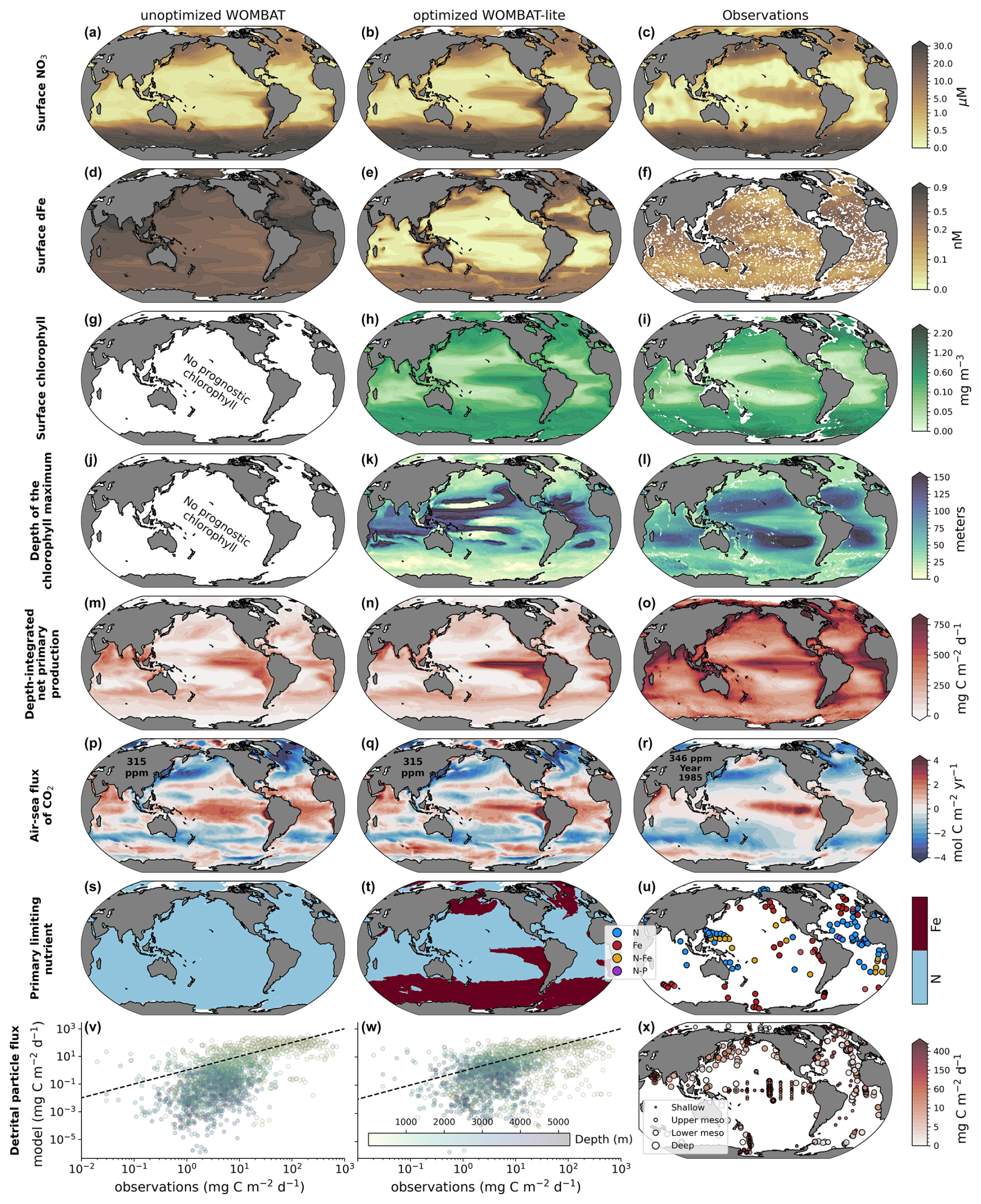
Figure 8 Comparison of the previous unoptimized WOMBAT (left) and WOMBAT-lite (middle) with the eight target observations (right). (a–c) Surface NO₃ concentration (µM). (d–f) Surface dFe concentration (nM). (g–i) Surface chlorophyll concentration (mg m⁻³). (j–l) Depth of the chlorophyll maximum (m). (m–o) Depth-integrated net primary production (mg C m⁻² d⁻¹). (p–r) Downward flux of CO₂ (mol C m⁻¹ yr⁻¹) (µM). (s–u) Primary limiting nutrient to phytoplankton growth at the surface. (v–x) Downward flux of particulate organic carbon (mg C m⁻¹ d⁻¹). We show annual means here even though statistical measures of performance shown in Fig. 6 are computed including temporal variations at a monthly resolution. Output after 100 years of forward simulation from initialization with repeat atmospheric forcing for calendar year 1990–1991 conditions using the JRA-55do (Tsujino et al., 2018). Atmospheric CO₂ set at 315 ppm in the experiments. Note that the ocean-only hindcast runs performed here with the previous, unoptimized WOMBAT used a parameter set detailed in Law et al. (2017) that is intended for the ACCESS-1.5 Earth system model.

3.4.3 Phytoplankton bloom phenology

A major update to WOMBAT-lite has been the inclusion of prognostic chlorophyll-to-carbon ratios within its phytoplankton functional type. This allows for direct comparison with remotely sensed chlorophyll products, including those that investigate the phenology of phytoplankton blooms (Nicholson et al., 2025). WOMBAT-lite was not optimized for its representation of phytoplankton phenology but nonetheless performs well with respect to the timing of its annual blooms (Fig. 9a, b). The model captures the sharp change in bloom initiation (using the cumulative sum method) between the subtropical and subpolar regimes in both hemispheres, with autumn–winter subtropical blooms and spring–summer polar blooms. WOMBAT-lite also shows a general increase in the duration of its blooms in the tropics compared to the polar regions (Fig. 9c, d), as well as increases in the mean and integrated chlorophyll concentrations in the polar and upwelling regions compared to the subtropical gyres (Fig. 9e–h).

That said, WOMBAT-lite shows some clear biases compared with the Nicholson et al. (2025) dataset, which was built from the Ocean Color – Climate Change Initiative remotely sensed chlorophyll product (Sathyendranath et al., 2019). Blooms at the poles start too early, and their duration is too long. Overly long blooms in the Southern Ocean contributed to an overestimate of mean and integrated concentrations of chlorophyll than that calculated by Nicholson et al. (2025) (Fig. 9i). This bias may be associated with an excess of dFe due to a ferricline that is placed too shallow (Fig. 8e, f), a common model bias (Tagliabue et al., 2016) that is also present in our simulations and which amplifies iron supply and chlorophyll accumulation. Meanwhile, in the subtropics and northern high latitudes, the phytoplankton blooms in WOMBAT-lite appear to be too low in mean and integrated chlorophyll (Fig. 9i). This is possibly caused by bloom durations that are too short in the subtropics (they are >300 d in the remote-sensing product), although this is not the case in the northern polar region. Equally, though, these biases in bloom chlorophyll metrics may be due to our optimization against a different chlorophyll product (Sauzède et al., 2016), with which the model shows good agreement. Alternatively, it is possible that representing the global marine phytoplankton community with only one functional type limits the model's potential to realize the full variation. Capturing the bloom phenology of phytoplankton is important because there is evidence of multi-decadal trends in their start, end and duration in both the Southern and Arctic oceans (Ardyna and Arrigo, 2020; Thomalla et al., 2023), and according to the results herein, the timing and duration of the bloom are influential to air–sea CO₂ fluxes.

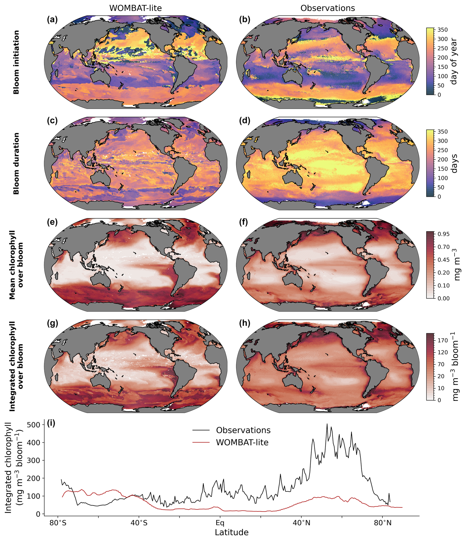
Figure 9 Comparison of WOMBAT-lite (left) with phenological indicators of the annual phytoplankton bloom observed via chlorophyll a (right). (a–b) Bloom initiation day. (c–d) Bloom duration (days). (e–f) Mean bloom chlorophyll a across duration (mg m⁻³). (g–h) Integrated bloom chlorophyll (mg m⁻³ bloom⁻¹). (i) Zonal mean integrated bloom chlorophyll for the observations (black) and WOMBAT-lite (red). Observations are provided by Nicholson et al. (2025). Phenological metrics are calculated via the cumulative sum method. For WOMBAT-lite these results come from the optimized model after 100 years of forward simulation from initialization with repeat atmospheric forcing for calendar year 1990–1991 conditions using the JRA-55do (Tsujino et al., 2018).

3.4.4 Carbon fluxes

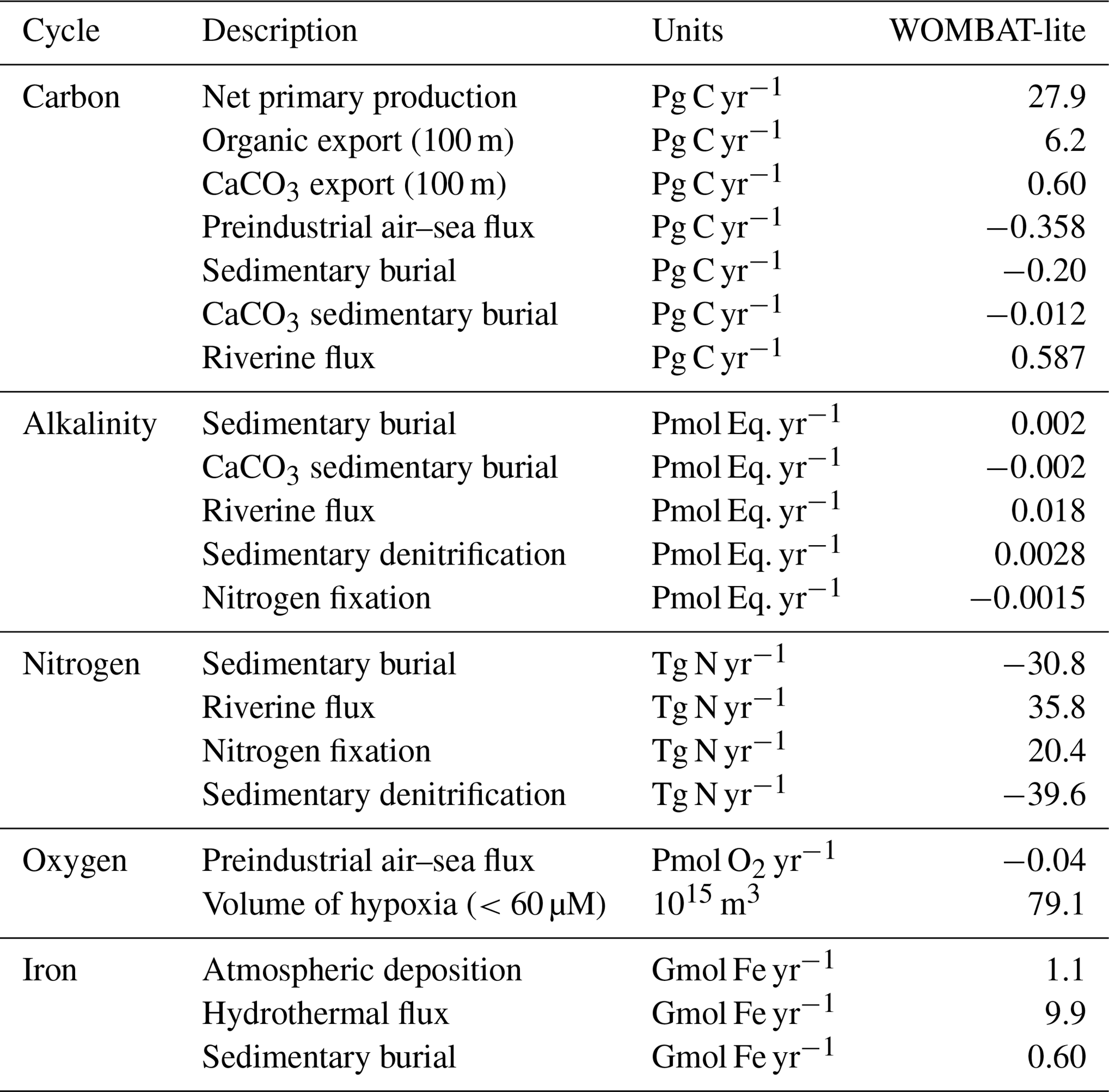
Previous assessments of ocean biogeochemical models show that the Southern Ocean air–sea CO₂ fluxes are strongly biased (Hauck et al., 2020, 2023a). We therefore sought to improve this aspect within WOMBAT-lite. To properly assess the performance of WOMBAT-lite for reproducing global CO₂ fluxes, we performed a hindcast simulation with the optimal version of WOMBAT-lite from 1958 to 2019 forced by the inter-annually changing JRA55-do atmospheric fields and with the historical increase in atmospheric CO₂. This hindcast simulation was initialized with biogeochemical fields at the end of a 200-year spin-up simulation with the same repeat “normal” year forcing of the JRA55-do (Stewart et al., 2020), with atmospheric CO₂ set at 315.2 ppm (equivalent calendar year 1957) and where Alk and preindustrial DIC budgets were at quasi-equilibrium. Budgets of major tracers at year 200 are presented in Table 3. This hindcast simulation did not strictly adhere to the recommendations of the OMIP2 protocol (Orr et al., 2017) but was sufficient to assess the seasonality of air–sea CO₂ fluxes in WOMBAT-lite.

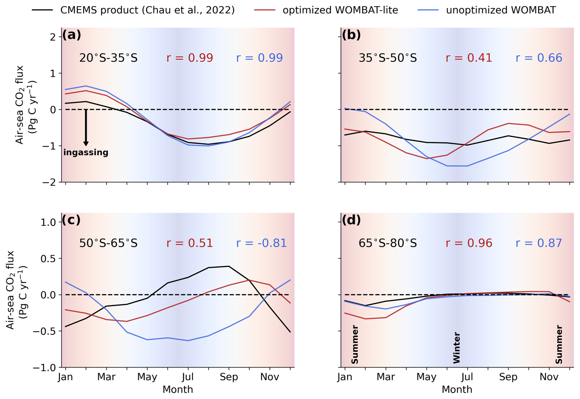
Figure 10 Climatological evolution of the integrated air–sea CO₂ flux over the latitudinal bands in the Southern Ocean averaged over the years 1990 to 2010. (a) Observational products from the Copernicus Marine Environmental Monitoring Service (black) are compared with fluxes from WOMBAT-lite (red) and an unoptimized, previous version of WOMBAT (blue) integrated between 20–35° S (subtropics). Pearson's correlations are shown for both models. Negative values are net ingassing of CO₂ into the ocean. Background shading denotes the seasonal transition from summer to winter to summer. Panels (b), (c) and (d) are the same as in (a) but integrated within 35–50° S for the subtropical–subantarctic transition, 50–65° S for the Antarctic Circumpolar Current and 65–80° S for Antarctic zone, respectively.

Table 3 Key rates in WOMBAT-lite after 200-year spin-up under repeat normal year forcing with optimized parameters.

We directly compared the monthly CO₂ fluxes between an observation product (Chau et al., 2022) and WOMBAT-lite as well as the unoptimized model from January 1985 to December 2018. With optimal parameters, WOMBAT-lite shows improvement in its seasonality and regional agreement of CO₂ fluxes compared with an unoptimized version of the model (Figs. 10, 11). While CO₂ fluxes are strongly controlled by thermal processes in the subtropics and are thus well approximated by optimized and unoptimized versions alike (Figs. 10a, 11), CO₂ fluxes at higher latitudes are, however, more affected by biological drawdown and release (Mongwe et al., 2018; Takahashi et al., 2002). In the transition from subtropical to subantarctic zones (35–50° S) the observations show overall oceanic uptake of CO₂, but importantly a greater uptake in the summer (Fig. 10b). Optimized WOMBAT-lite manages to show some improvement over the unoptimized model, with lower uptake in the winter and a trend towards uptake in the spring/summer. Nonetheless, this improvement is marginal in this zone and suggests that further improvement can be made in the future. The best match between WOMBAT-lite and the data is achieved in the Antarctic Circumpolar Current zone (50–65° S), where WOMBAT-lite shows good climatological correlations with the observations, while the unoptimized model shows negative correlations (Figs. 10c, 11). The flip from poor to good performance is caused by the net outgassing in the late winter and a trend towards oceanic uptake in the spring/summer (Fig. 10c). Better seasonal correlations (0.87→0.96) are also achieved in the Antarctic zone (65–80° S), although with WOMBAT-lite potentially overestimating the summer flux of CO₂ into these waters (Fig. 10d).

Improvement in air–sea CO₂ fluxes is noteworthy from a zonally integrated perspective that incorporates the Northern Hemisphere (Fig. 12). North of 40° N, the oceanic uptake of CO₂ in the unoptimized version of the model exceeded the observations, and this is somewhat reduced in WOMBAT-lite due to a substantial reduction in winter ingassing (Fig. 12b), while summer uptake is increased (Fig. 12c), resulting in a better match to observed CO₂ fluxes in the Northern Hemisphere (Fig. 12a) that is also visible in the temporal correlations (Fig. 11). Meanwhile, there is little difference between the optimized and unoptimized versions of the model in the low latitudes, emphasizing how thermal changes dominate air–sea CO₂ fluxes in this region (Takahashi et al., 2002). Once again, in the Southern Ocean, we see clear improvements from a zonally integrated perspective. Winter outgassing is now achieved in WOMBAT-lite, although the zone of peak outgassing occurs too far north (Fig. 12c). Similarly, summer oceanic uptake is now achieved and is a closer match to the observations, although again the zones of maximum uptake are shifted too far north by roughly ∼5° (Fig. 12b). Overall, the changes in the biogeochemical functionality of WOMBAT-lite show some improvements in reproducing observed air–sea CO₂ fluxes, although we note some degree of caution is required given the uncertainty in the observationally based product itself (Gloege et al., 2021; Hauck et al., 2023b).

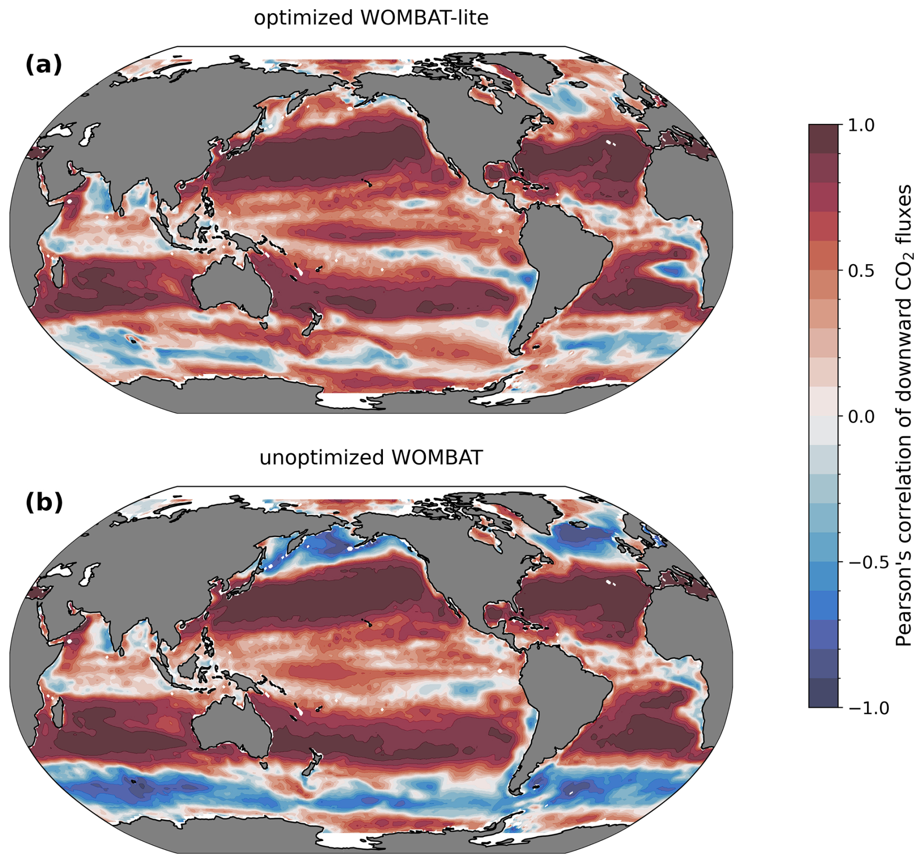
Figure 11 Temporal correlations in monthly CO₂ fluxes with an observation product (Chau et al., 2022). (a) Optimized WOMBAT-lite and (b) unoptimized, previous WOMBAT over the years 1985 to 2019.

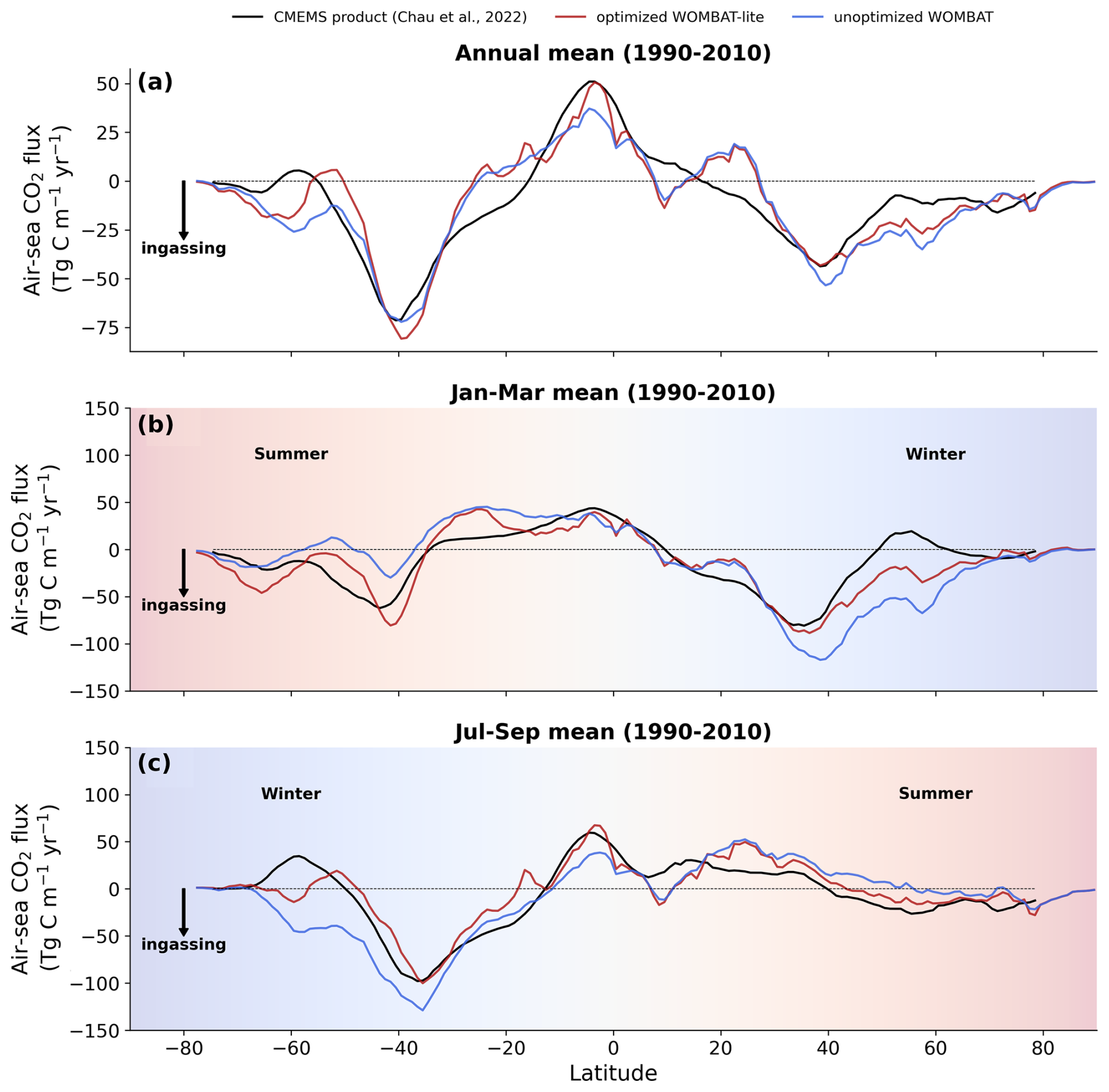
Figure 12 Zonally integrated air–sea CO₂ fluxes. (a) Annual mean observations (black) averaged over the years 1990–2010 are compared with fluxes from WOMBAT-lite (red) and a previous, unoptimized version of WOMBAT (blue). Panels (b) and (c) are the same as in (a) but are averages over the months of January–March and July–September, respectively. Positive fluxes are out of the ocean.

4 Summary

We have updated the World Ocean Model of Biogeochemistry and Trophic dynamics (WOMBAT) in a new version called WOMBAT-lite (see Sect. 2). These updates necessitated optimization of the many new and existing model parameters. To do so, we used a surrogate machine learning model trained on a limited sample of real model output that provided many synthetic estimates of model performance (i.e., global NRMSE and the global cost function) at low computation cost. It is critical for accurate global sensitivity analysis (Saltelli et al., 2019) and Bayesian parameter optimization techniques (Reddy et al., 2024a) to have many samples. These surrogate-based sensitivity analyses and parameter optimization techniques are therefore gaining traction in climate and environmental sciences where computational overhead severely restricts the number of direct model simulations that can be done (Li et al., 2018; Reddy et al., 2024a, b; Williamson et al., 2017; Xu et al., 2022, 2018). Ocean biogeochemical models are no different. Here we applied the surrogate-based method to WOMBAT-lite, optimized the model parameters and delivered improved performance in reproducing eight target datasets.

Other approaches do exist for optimization of biogeochemical models, such as iterative ensemble methods (Singh et al., 2025), which do not rely on surrogate methods but instead use ensembles to iteratively adjust either the initial state or the parameters towards their optimal values through regular data assimilation (Dowd et al., 2014). Similarly, the emergence of machine learning emulators (Eyring et al., 2024) that resolve the full spatiotemporal field of the target datasets could be used to assess performance and optimize parameters. While these approaches can provide optimal parameter values that evolve in time and/or space, the surrogate approach employed herein represents a simple yet valid approach that provides globally optimized parameter values that are fixed in time and space, but importantly without large computation overhead. Once the surrogate is trained, it can be deployed cheaply to explore the parameter space in different ways, offering flexibility to select a new set of parameters with perhaps an emphasis on one target field (e.g., air–sea CO₂ flux) over another, if required. One disadvantage, however, is that the optimization can only be as good as the skill of the surrogate, meaning that careful training is critical.

The improvements showcased herein included surface distributions of dFe and NO₃; surface chlorophyll concentrations; the representation of deep chlorophyll maximums; phytoplankton phenology; and particularly the seasonality of air–sea CO₂ fluxes in the high latitudes, where in some regions the seasonality flipped from a negative correlation in the unoptimized model to a positive correlation with our new, optimized model. Surface chlorophyll was also well reproduced, as was the distribution of iron-limited regions of primary productivity. Additionally, global net primary production was increased by 50 %, partially rectifying a low bias in the previous unoptimized model, although our simulated rate of 28 Pg C yr⁻¹ remains low compared with data-based estimates of ∼ 50 Pg C yr⁻¹ (Buitenhuis et al., 2013).

Despite these improvements, biases do remain. Chief among them is a difficulty in reproducing the seasonality of air–sea CO₂ exchange in the Southern Ocean, despite the improvements achieved here. WOMBAT-lite does manage to represent the austral winter outgassing of CO₂ from the polar frontal region but fails to absorb enough CO₂ in the summer, particularly in the subantarctic zone. Other models struggle with representing the seasonality of CO₂ exchange in the Southern Ocean, with some absorbing too much (e.g., Yool et al., 2021) and others, like WOMBAT-lite, too little (see Hauck et al., 2020, 2023a). Physical biases in the model are no doubt important here, such as those that have insufficient winter mixing, as has been proposed (Hauck et al., 2023a). Our sensitivity analysis and optimization procedure, however, would also suggest that how we choose to represent the biology contributes substantially to model skill in air–sea CO₂ fluxes (also see Mongwe et al., 2018). Two parameters of importance for Southern Ocean CO₂ fluxes were optimized at the lower edge of their a priori ranges: the linear mortality coefficient for phytoplankton (${\mathit{\gamma }}_{\mathrm{p}}^{\mathrm{0}}$) and the prey capture rate coefficient of zooplankton (ε). This suggests that further improvement in Southern Ocean CO₂ fluxes can be gained by exploring lower values for these parameters than those explored here. Alternatively, spatial variations in ε that capture transitions from nano- to meso-zooplankton from oligotrophic to eutrophic regimes (Rohr et al., 2024) may serve to accelerate the phytoplankton bloom at the beginning of the growth season. Furthermore, the succession of different types of phytoplankton is important for the biological carbon pump (Tréguer et al., 2018). Therefore, representing these shifts in community with additional functional types of plankton beyond that explored herein might be important for the phenology of the annual spring bloom and by extension Southern Ocean CO₂ fluxes. According to a recent analysis, this phenology is changing (Thomalla et al., 2023), which may imply a changing strength and/or seasonality of air–sea CO₂ fluxes in the region.

As a final word, we note that a surrogate-based optimization of a complex numerical model can only be as good as the initial sample set on which the surrogate is trained. A clear example of this limitation is evident in Fig. 7. Even with its optimal parameters, WOMBAT-lite suffered a loss in performance when run over 100 years compared to when run over only 10 years. Future iterations of surrogate-based optimization would therefore benefit from extending the length of simulations done by the initial set of sensitivity experiments. That said, significant savings in computation efficiency would be needed before this is possible with computationally demanding models, such as ocean biogeochemical models, in particular those involving more plankton functional groups and thus many more uncertain parameters, but could be feasible by running the biogeochemical model offline from the ocean physics (e.g., Séférian et al., 2013). This approach would also eliminate any confounding errors caused by an evolution of the ocean's physical state since the physical state would not be allowed to evolve. Future versions of WOMBAT, including WOMBAT-lite, WOMBAT-mid and WOMBAT-full, and their deployment into different configurations (e.g., higher-resolution versions) would benefit from this approach.

Appendix A

A1 Key equations of the previous WOMBAT

The previous version of WOMBAT is a simple nutrient–phytoplankton–zooplankton–detritus model (Law et al., 2017; Oke et al., 2013) simulating the biomass pools of one phytoplankton, one zooplankton and one detrital functional type; two nutrients of phosphate *16, which is often referred to conveniently as nitrate, (NO₃, mmol m⁻³) and dissolved iron (dFe; µmol m⁻³); the carbonate system (DIC, Alk and CaCO₃; mmol C m⁻³); and dissolved oxygen (mmol O₂ m⁻³). The basic currency of the ecosystem component is 16 times phosphorus (i.e., nitrogen but without external sources and sinks). Biological stoichiometry is fixed at a $\mathrm{C}:\mathrm{N}:{\mathrm{O}}_{\mathrm{2}}$ ratio of $\mathrm{106}:\mathrm{16}:-\mathrm{172}$, and the Fe:N of phytoplankton is 20:1 µmol : mol. The minimum of nutrient availability or availability of photosynthetically active radiation (PAR; W m⁻²) controls phytoplankton growth rates. Growth of phytoplankton is calculated by first solving for a maximum growth rate (μ^max; d⁻¹), dependent on temperature (T; °C), and then applying the minimum of nutrient (L^nutrient) and light (L^PAR) limitation terms to scale down from the maximum to a realized growth rate (μ; d⁻¹).

The budgets for the previous WOMBAT are as follows:

$$\begin{array}{}\text{(A1)}& {\displaystyle \frac{\partial {\mathrm{NO}}_{\mathrm{3}}}{\partial t}}={\mathit{\gamma }}_{\mathrm{d}}+{\mathit{\gamma }}_{\mathrm{z}}+{\mathit{\gamma }}_{\mathrm{p}}-\mathit{\mu }{B}_{\mathrm{p}},\text{(A2)}& {\displaystyle \frac{\partial \mathrm{dFe}}{\partial t}}=\left({\mathit{\gamma }}_{\mathrm{d}}+{\mathit{\gamma }}_{\mathrm{z}}+{\mathit{\gamma }}_{\mathrm{p}}-\mathit{\mu }{B}_{\mathrm{p}}\right)\left({\displaystyle \frac{\mathrm{Fe}}{\mathrm{N}}}\right)-\mathrm{scavenging},\text{(A3)}& {\displaystyle \frac{\partial {\mathrm{O}}_{\mathrm{2}}}{\partial t}}=\left(\mathit{\mu }{B}_{\mathrm{p}}-{\mathit{\gamma }}_{\mathrm{d}}-{\mathit{\gamma }}_{\mathrm{z}}-{\mathit{\gamma }}_{\mathrm{p}}\right)\left({\displaystyle \frac{{\mathrm{O}}_{\mathrm{2}}}{\mathrm{N}}}\right),\text{(A4)}& {\displaystyle \frac{\partial B_{\mathrm{p}}}{\partial t}}=\mathit{\mu }{B}_{\mathrm{p}}-{\mathit{\gamma }}_{\mathrm{p}}-{\mathrm{\Gamma }}_{\mathrm{p}}-g{B}_{\mathrm{z}},\text{(A5)}& {\displaystyle \frac{\partial B_{\mathrm{z}}}{\partial t}}=g{B}_{\mathrm{z}}\mathit{\lambda }-{\mathit{\gamma }}_{\mathrm{z}}-{\mathrm{\Gamma }}_{\mathrm{z}},\text{(A6)}& {\displaystyle \frac{\partial B_{\mathrm{d}}}{\partial t}}={\mathrm{\Gamma }}_{\mathrm{p}}+{\mathrm{\Gamma }}_{\mathrm{z}}+g{B}_{\mathrm{z}}\left(\mathrm{1}-\mathit{\lambda }\right)-{\mathit{\gamma }}_{\mathrm{d}},\text{(A7)}& {\displaystyle }\begin{array}{rl}{\displaystyle \frac{\partial B_{{\mathrm{CaCO}}_{\mathrm{3}}}}{\partial t}}& =\left({\mathrm{\Gamma }}_{\mathrm{p}}+{\mathrm{\Gamma }}_{\mathrm{z}}+g{B}_{\mathrm{z}}\left(\mathrm{1}-\mathit{\lambda }\right)\right)\\ & \cdot \left({\displaystyle \frac{\mathrm{C}}{\mathrm{N}}}\right)f_{\mathrm{inorg}}-{\mathit{\gamma }}_{{\mathrm{CaCO}}_{\mathrm{3}}},\end{array}\text{(A8)}& {\displaystyle }\begin{array}{rl}{\displaystyle \frac{\partial \mathrm{DIC}}{\partial t}}& =\left({\mathit{\gamma }}_{\mathrm{d}}+{\mathit{\gamma }}_{\mathrm{z}}+{\mathit{\gamma }}_{\mathrm{p}}-\mathit{\mu }{B}_{\mathrm{p}}\right)\left({\displaystyle \frac{\mathrm{C}}{\mathrm{N}}}\right)\\ & -(\left({\mathrm{\Gamma }}_{\mathrm{p}}+{\mathrm{\Gamma }}_{\mathrm{z}}+g{B}_{\mathrm{z}}\left(\mathrm{1}-\mathit{\lambda }\right)\right)\\ & \cdot \left({\displaystyle \frac{\mathrm{C}}{\mathrm{N}}}\right)f_{\mathrm{inorg}}-{\mathit{\gamma }}_{{\mathrm{CaCO}}_{\mathrm{3}}}),\end{array}\text{(A9)}& {\displaystyle }\begin{array}{rl}{\displaystyle \frac{\partial \mathrm{Alk}}{\partial t}}& =-\left({\mathit{\gamma }}_{\mathrm{d}}+{\mathit{\gamma }}_{\mathrm{z}}+{\mathit{\gamma }}_{\mathrm{p}}-\mathit{\mu }{B}_{\mathrm{p}}\right)\\ & -\mathrm{2}(\left({\mathrm{\Gamma }}_{\mathrm{p}}+{\mathrm{\Gamma }}_{\mathrm{z}}+g{B}_{\mathrm{z}}\left(\mathrm{1}-\mathit{\lambda }\right)\right)\\ & \cdot \left({\displaystyle \frac{\mathrm{C}}{\mathrm{N}}}\right)f_{\mathrm{inorg}}-{\mathit{\gamma }}_{{\mathrm{CaCO}}_{\mathrm{3}}}).\end{array}\end{array}$$

Regarding phytoplankton growth rates (μ; d⁻¹) the individual terms are

$$\begin{array}{}\text{(A10)}& {\displaystyle }{\mathit{\mu }}^{\max }=\mathit{\alpha }{\mathit{\beta }}^{\left(T\right)},\text{(A11)}& {\displaystyle }{L}^{\mathrm{PAR}}=(\mathrm{1}-e^{-\frac{\mathrm{PI}\cdot \mathrm{PAR}}{{\mathit{\mu }}^{\max }}}),\text{(A12)}& {\displaystyle }{L}^{\mathrm{nutrient}}=min\left({\displaystyle \frac{{\mathrm{NO}}_{\mathrm{3}}}{{\mathrm{NO}}_{\mathrm{3}}+K^{\mathrm{N}}}},{\displaystyle \frac{\mathrm{dFe}}{\mathrm{dFe}+K^{\mathrm{Fe}}}}\right),\text{(A13)}& {\displaystyle }\mathit{\mu }=min({\mathit{\mu }}^{\max }{L}^{\mathrm{PAR}},{\mathit{\mu }}^{\max }{L}^{\mathrm{nutrient}}),\end{array}$$

where α and β control the non-linear temperature-dependency of phytoplankton metabolism (Eppley, 1972), PI is the slope of the photosynthesis–irradiance curve (mg N (mg Chl)⁻¹ (W m⁻²)⁻¹ d⁻¹), and K^N and K^Fe are the half-saturation coefficients for nutrient limitation by NO₃ and dFe (mmol m⁻³ and µmol m⁻³, respectively). The realized growth of phytoplankton (μ; d⁻¹) is multiplied by their biomass (B_p; mmol N m⁻³) to retrieve growth of phytoplankton (mmol N m⁻³ d⁻¹). PAR is solved for as 43 % of incoming shortwave radiation and then attenuated at a constant rate through the water column.

Phytoplankton mortality occurs via zooplankton grazing, as well as linear (γ) and quadratic (Γ) mortality terms. The specific grazing rate for zooplankton (g; d⁻¹) is described by a type III disk equation (Gentleman and Neuheimer, 2008)

$$\begin{array}{}\text{(A14)}& g={\displaystyle \frac{g^{\max }\mathit{\epsilon }{B}_{\mathrm{p}}^{\mathrm{2}}}{g^{\max }+\mathit{\epsilon }{B}_{\mathrm{p}}^{\mathrm{2}}}},\end{array}$$

where g^max is the constant, temperature-independent, maximum (prey replete) specific grazing rate in units of d⁻¹, and ε describes how fast the prey capture rates increase with the ambient phytoplankton (or prey) concentration in units of (mmol N m⁻³)⁻² d⁻¹ (Rohr et al., 2022). Phytoplankton losses to grazing then occur according to the product of g and zooplankton biomass (B_z; mmol N m⁻³). A fraction of the grazed phytoplankton biomass is routed to zooplankton according to gB_zλ, where λ is the assimilation efficiency (akin to gross growth efficiency). The fraction that is not assimilated into zooplankton (1−λ) is routed to detritus (B_d; mmol N m⁻³). Linear mortality is temperature-dependent, such that

$$\begin{array}{}\text{(A15)}& {\mathit{\gamma }}_{\mathrm{p}}={\mathit{\gamma }}_{\mathrm{p}}^{\mathrm{0}}{B}_{\mathrm{p}}{\mathit{\beta }}^T,\end{array}$$

whereas quadratic mortality is density-dependent, but temperature-independent, such that

$$\begin{array}{}\text{(A16)}& {\mathrm{\Gamma }}_{\mathrm{p}}={\mathrm{\Gamma }}_{\mathrm{p}}^{\mathrm{0}}{B}_{\mathrm{p}}^{\mathrm{2}}.\end{array}$$

Both ${\mathit{\gamma }}_{\mathrm{p}}^{\mathrm{0}}$ and ${\mathrm{\Gamma }}_{\mathrm{p}}^{\mathrm{0}}$ are constant parameters in units of d⁻¹ and m³ mmol⁻¹ d⁻¹, respectively. Zooplankton are also affected by linear (γ_z) and quadratic (Γ_z) mortality terms of the same form according to predefined values of ${\mathit{\gamma }}_{\mathrm{z}}^{\mathrm{0}}$ and ${\mathrm{\Gamma }}_{\mathrm{z}}^{\mathrm{0}}$. All quadratic mortality of phytoplankton and zooplankton biomass is routed to detritus, while linear mortality losses are routed to dissolved nutrients and inorganic carbon. Remineralization of detritus follows the same form as linear mortality (Eq. A15), with its own rate controlled by the ${\mathit{\gamma }}_{\mathrm{d}}^{\mathrm{0}}$ coefficient, which is halved at depths below 180 m.

Both detritus and CaCO₃ sink at constant rates. CaCO₃ is produced at the same time as detritus (i.e., via unassimilated phytoplankton and quadratic mortality losses of phytoplankton and zooplankton), but at a constant rate controlled by f_inorg, which is equal to 6.2 % of the organic detritus being produced. In contrast to the detrital pool, the CaCO₃ pool ($B_{{\mathrm{CaCO}}_{\mathrm{3}}}$; mmol C m⁻³) is remineralized (dissolved) at a constant rate (${\mathit{\gamma }}_{{\mathrm{CaCO}}_{\mathrm{3}}}$) that is not temperature-dependent.

In addition to its biological cycling, dFe is affected by abiotic scavenging. This is represented implicitly via a relaxation term ($K_{\mathrm{scav}}^{\mathrm{dFe}}$; d⁻¹) to a background dFe concentration set by an assumed concentration of ligand-bound iron (Fe_Lig; µmol m⁻³), where

$$\begin{array}{}\text{(A17)}& \mathrm{Scavenging}=K_{\mathrm{scav}}^{\mathrm{dFe}}\cdot max(\mathrm{0},\text{dFe}-{\mathrm{Fe}}_{\mathrm{Lig}}).\end{array}$$

dFe is also reduced to a maximum of 1 µmol m⁻³ at the continental shelves, where the sediments are less than 200 m deep.

A2 Key equations of WOMBAT-lite

The budgets for the full set of ecosystem equations of WOMBAT-lite are as follows:

$$\begin{array}{}\text{(A18)}& {\displaystyle \frac{\partial {\mathrm{NO}}_{\mathrm{3}}}{\partial t}}=\left({\mathit{\gamma }}_{\mathrm{d}}+{\mathit{\gamma }}_{\mathrm{z}}+{\mathit{\gamma }}_{\mathrm{p}}-\mathit{\mu }{B}_{\mathrm{p}}\right)\left({\displaystyle \frac{\mathrm{N}}{\mathrm{C}}}\right),\text{(A19)}& {\displaystyle }\begin{array}{rl}{\displaystyle \frac{\partial \mathrm{dFe}}{\partial t}}& =\left({\mathit{\gamma }}_{\mathrm{d}}{Q}_{\mathrm{d}}^{\frac{\mathrm{Fe}}{\mathrm{C}}}+{\mathit{\gamma }}_{\mathrm{z}}{Q}_{\mathrm{z}}^{\frac{\mathrm{Fe}}{\mathrm{C}}}+{\mathit{\gamma }}_{\mathrm{p}}{Q}_{\mathrm{p}}^{\frac{\mathrm{Fe}}{\mathrm{C}}}-{\mathit{\mu }}_{\mathrm{Fe}}\right)\\ & \cdot \mathrm{1000}-{\mathrm{Fe}}_{\mathrm{precip}}^{\mathrm{dFe}\to }-{\mathrm{Fe}}_{\mathrm{scav}}^{\mathrm{dFe}\to }-{\mathrm{Fe}}_{\mathrm{coag}}^{\mathrm{dFe}\to B_{\mathrm{d}}^{\mathrm{Fe}}},\end{array}\text{(A20)}& {\displaystyle \frac{\partial {\mathrm{O}}_{\mathrm{2}}}{\partial t}}=\left(\mathit{\mu }{B}_{\mathrm{p}}-{\mathit{\gamma }}_{\mathrm{d}}-{\mathit{\gamma }}_{\mathrm{z}}-{\mathit{\gamma }}_{\mathrm{p}}\right)\left({\displaystyle \frac{{\mathrm{O}}_{\mathrm{2}}}{\mathrm{C}}}\right),\text{(A21)}& {\displaystyle \frac{\partial B_{\mathrm{p}}}{\partial t}}=\mathit{\mu }{B}_{\mathrm{p}}-{\mathit{\gamma }}_{\mathrm{p}}-{\mathrm{\Gamma }}_{\mathrm{p}}-g{B}_{\mathrm{z}}\left({\displaystyle \frac{B_{\mathrm{p}}}{B_{\mathrm{prey}}}}\right),\text{(A22)}& {\displaystyle \frac{\partial B_{\mathrm{p}}^{\mathrm{Fe}}}{\partial t}}={\mathit{\mu }}_{\mathrm{Fe}}-\left({\mathit{\gamma }}_{\mathrm{p}}+{\mathrm{\Gamma }}_{\mathrm{p}}+g{B}_{\mathrm{z}}\left({\displaystyle \frac{B_{\mathrm{p}}}{B_{\mathrm{prey}}}}\right)\right)Q_{\mathrm{p}}^{\frac{\mathrm{Fe}}{\mathrm{C}}},\text{(A23)}& {\displaystyle \frac{\partial B_{\mathrm{p}}^{\mathrm{Chl}}}{\partial t}}={\mathit{\mu }}_{\mathrm{Chl}}-\mathrm{12}\left({\mathit{\gamma }}_{\mathrm{p}}+{\mathrm{\Gamma }}_{\mathrm{p}}+g{B}_{\mathrm{z}}\left({\displaystyle \frac{B_{\mathrm{p}}}{B_{\mathrm{prey}}}}\right)\right)Q_{\mathrm{p}}^{\frac{\mathrm{Chl}}{\mathrm{C}}},\text{(A24)}& {\displaystyle \frac{\partial B_{\mathrm{z}}}{\partial t}}=g{B}_{\mathrm{z}}\mathit{\lambda }-{\mathit{\gamma }}_{\mathrm{z}}-{\mathrm{\Gamma }}_{\mathrm{z}},\text{(A25)}& {\displaystyle }\begin{array}{rl}{\displaystyle \frac{\partial B_{\mathrm{z}}^{\mathrm{Fe}}}{\partial t}}& =g{B}_{\mathrm{z}}\mathit{\lambda }\left({\displaystyle \frac{B_{\mathrm{p}}}{B_{\mathrm{prey}}}}\right)Q_{\mathrm{p}}^{\frac{\mathrm{Fe}}{\mathrm{C}}}+g{B}_{\mathrm{z}}\mathit{\lambda }\left({\displaystyle \frac{{\mathit{\phi }}_{\mathrm{z}}^{\mathrm{d}}{B}_{\mathrm{d}}}{B_{\mathrm{prey}}}}\right)Q_{\mathrm{d}}^{\frac{\mathrm{Fe}}{\mathrm{C}}}\\ & -\left({\mathit{\gamma }}_{\mathrm{z}}+{\mathrm{\Gamma }}_{\mathrm{z}}\right)Q_{\mathrm{z}}^{\frac{\mathrm{Fe}}{\mathrm{C}}},\end{array}\text{(A26)}& {\displaystyle \frac{\partial B_{\mathrm{d}}}{\partial t}}={\mathrm{\Gamma }}_{\mathrm{p}}+{\mathrm{\Gamma }}_{\mathrm{z}}+g{B}_{\mathrm{z}}\left(\mathrm{1}-\mathit{\lambda }\right)-{\mathit{\gamma }}_{\mathrm{d}}-g{B}_{\mathrm{z}}\left({\displaystyle \frac{{\mathit{\phi }}_{\mathrm{z}}^{\mathrm{d}}{B}_{\mathrm{d}}}{B_{\mathrm{prey}}}}\right),\text{(A27)}& {\displaystyle }\begin{array}{rl}{\displaystyle \frac{\partial B_{\mathrm{d}}^{\mathrm{Fe}}}{\partial t}}& ={\mathrm{\Gamma }}_{\mathrm{p}}{Q}_{\mathrm{p}}^{\frac{\mathrm{Fe}}{\mathrm{C}}}+{\mathrm{\Gamma }}_{\mathrm{z}}{Q}_{\mathrm{z}}^{\frac{\mathrm{Fe}}{\mathrm{C}}}+g{B}_{\mathrm{z}}\left(\mathrm{1}-\mathit{\lambda }\right)\left({\displaystyle \frac{B_{\mathrm{p}}}{B_{\mathrm{prey}}}}\right)Q_{\mathrm{p}}^{\frac{\mathrm{Fe}}{\mathrm{C}}}\\ & +g{B}_{\mathrm{z}}\left(\mathrm{1}-\mathit{\lambda }\right)\left({\displaystyle \frac{{\mathit{\phi }}_{\mathrm{z}}^{\mathrm{d}}{B}_{\mathrm{d}}}{B_{\mathrm{prey}}}}\right)Q_{\mathrm{d}}^{\frac{\mathrm{Fe}}{\mathrm{C}}}\\ & -\left({\mathit{\gamma }}_{\mathrm{d}}+g{B}_{\mathrm{z}}\left({\displaystyle \frac{{\mathit{\phi }}_{\mathrm{z}}^{\mathrm{d}}{B}_{\mathrm{d}}}{B_{\mathrm{prey}}}}\right)\right)Q_{\mathrm{d}}^{\frac{\mathrm{Fe}}{\mathrm{C}}},\end{array}\text{(A28)}& {\displaystyle }\begin{array}{rl}{\displaystyle \frac{\partial B_{{\mathrm{CaCO}}_{\mathrm{3}}}}{\partial t}}& =\left({\mathrm{\Gamma }}_{\mathrm{p}}+{\mathrm{\Gamma }}_{\mathrm{z}}+g{B}_{\mathrm{z}}\left(\mathrm{1}-\mathit{\lambda }\right)\left({\displaystyle \frac{B_{\mathrm{p}}}{B_{\mathrm{prey}}}}\right)\right)\\ & \cdot f_{\mathrm{inorg}}-{\mathit{\gamma }}_{{\mathrm{CaCO}}_{\mathrm{3}}},\end{array}\text{(A29)}& {\displaystyle }\begin{array}{rl}{\displaystyle \frac{\partial \mathrm{DIC}}{\partial t}}& =\left({\mathit{\gamma }}_{\mathrm{d}}+{\mathit{\gamma }}_{\mathrm{z}}+{\mathit{\gamma }}_{\mathrm{p}}-\mathit{\mu }{B}_{\mathrm{p}}\right)\\ & -(\left({\mathrm{\Gamma }}_{\mathrm{p}}+{\mathrm{\Gamma }}_{\mathrm{z}}+g{B}_{\mathrm{z}}\left(\mathrm{1}-\mathit{\lambda }\right)\left({\displaystyle \frac{B_{\mathrm{p}}}{B_{\mathrm{prey}}}}\right)\right)\\ & \cdot f_{\mathrm{inorg}}-{\mathit{\gamma }}_{{\mathrm{CaCO}}_{\mathrm{3}}}),\end{array}\text{(A30)}& {\displaystyle }\begin{array}{rl}{\displaystyle \frac{\partial \mathrm{Alk}}{\partial t}}& =-\left({\mathit{\gamma }}_{\mathrm{d}}+{\mathit{\gamma }}_{\mathrm{z}}+{\mathit{\gamma }}_{\mathrm{p}}-\mathit{\mu }{B}_{\mathrm{p}}\right)\\ & -\mathrm{2}(\left({\mathrm{\Gamma }}_{\mathrm{p}}+{\mathrm{\Gamma }}_{\mathrm{z}}+g{B}_{\mathrm{z}}\left(\mathrm{1}-\mathit{\lambda }\right)\left({\displaystyle \frac{B_{\mathrm{p}}}{B_{\mathrm{prey}}}}\right)\right)\\ & \cdot f_{\mathrm{inorg}}-{\mathit{\gamma }}_{{\mathrm{CaCO}}_{\mathrm{3}}}).\end{array}\end{array}$$

A2.1 Phytoplankton growth

Growth of phytoplankton (B_p) is controlled by a combination of temperature, light and nutrient supply. Temperature, T (°C), sets the maximum potential growth rate of phytoplankton, μ^max (d⁻¹), following the Eppley curve (Eppley, 1972),

$$\begin{array}{}\text{(A31)}& {\mathit{\mu }}^{\max }={\mathit{\alpha }}_{\mathrm{a}}{\mathit{\beta }}_{\mathrm{a}}^{\left(T\right)},\end{array}$$

where both α_a and β_a (subscript a for autotrophy) are predefined (Table 1).

A2.2 Phytoplankton growth: light limitation

Incoming shortwave radiation at the surface (W m⁻²) is multiplied by 0.43 to return the photosynthetically active radiation (PAR), which is further split into three major wavelength bands associated with blue, green and red light. Each band has unique attenuation through the water column according to the power law coefficients (χ and e) provided by Morel and Maritorena (2001) in their Table 2, which change depending on the chlorophyll concentration and implicitly account for the packaging effect of larger cells, assuming that more chlorophyll brings with it an increase in the mean community cell size. Attenuation of blue, green and red light is increased as chlorophyll concentrations increase, but as cells grow larger they absorb less light per unit chlorophyll. We calculate the depth of the euphotic zone to be the depth at which PAR is 1 % of its incident intensity, resulting in typical depths between 50 and 150 m.

The maximum potential growth rate is multiplied by a light limitation term, L^PAR, to return light-limited primary production, μ^PAR. L^PAR depends on the availability of PAR, the ratio of the euphotic depth to mixed layer depth ($\frac{z_{\mathrm{eup}}}{z_{\mathrm{MLD}}}$), the linear mortality rate (γ; d⁻¹) and the chlorophyll quota of the cell ($Q^{\frac{\mathrm{Chl}}{\mathrm{C}}}$; mg mg⁻¹). First, we solve for the initial slope of the photosynthesis–irradiance curve, PI, which is altered by $Q^{\frac{\mathrm{Chl}}{\mathrm{C}}}$ such that

$$\begin{array}{}\text{(A32)}& \mathrm{PI}={\mathrm{PI}}^{\mathrm{0}}{Q}^{\frac{\mathrm{Chl}}{\mathrm{C}}},\end{array}$$

where PI⁰ can be altered to increase or decrease the response of phytoplankton to light. Following PI, we calculate L^PAR via

$$\begin{array}{}\text{(A33)}& {\displaystyle }{L}^{\mathrm{PAR}}=\left(\mathrm{1}-e^{-\frac{\mathrm{PI}\cdot \mathrm{PAR}}{\mathrm{1}+{\mathit{\gamma }}_{\mathrm{p}}}}\right)L^{\mathrm{eup}},\text{(A34)}& {\displaystyle }{L}^{\mathrm{eup}}=min\left(\mathrm{1},{\displaystyle \frac{z_{\mathrm{eup}}}{z_{\mathrm{MLD}}}}\right),\end{array}$$

where L^eup is scaled down when the mixed layer is deeper than the euphotic zone, representing the disadvantageous mixing of cells into darkness due to deep mixed layers. Light-limited phytoplankton growth, μ^PAR (mmol C m⁻³ d⁻¹), is then

$$\begin{array}{}\text{(A35)}& {\mathit{\mu }}^{\mathrm{PAR}}={\mathit{\mu }}^{\max }{L}^{\mathrm{PAR}}.\end{array}$$

A2.3 Phytoplankton growth: nutrient limitation

The minimum of multiple nutrient limitation terms (L^nutrient) is then multiplied against μ^PAR to return the realized growth rate, μ (d⁻¹):

$$\begin{array}{}\text{(A36)}& \mathit{\mu }={\mathit{\mu }}^{\mathrm{PAR}}{L}^{\mathrm{nutrient}}={\mathit{\mu }}^{\max }{L}^{\mathrm{PAR}}{L}^{\mathrm{nutrient}}.\end{array}$$

The limitation terms include growth limitation by nitrogen (L^N) and dFe (L^Fe), such that

$$\begin{array}{}\text{(A37)}& L^{\mathrm{nutrient}}=min\left(L^{\mathrm{N}}{L}^{\mathrm{Fe}}\right).\end{array}$$

The nutrient limitation terms are dependent on the availability of the resource, R, and the half-saturation coefficient for uptake of that resource by the phytoplankton ($K_{\mathrm{p}}^R$), which itself is dependent on the biomass of phytoplankton in terms of carbon (B_p). Initial $K_{\mathrm{p}}^R$ values are predefined ($K_{\mathrm{p}}^{R_{\mathrm{0}}}$; Table 1) but are made to vary with phytoplankton biomass. We relate the biomass concentration of phytoplankton to the mean community cell size, which then affects the half-saturation coefficients for resource uptake. Using compilations of marine phytoplankton and zooplankton communities, Wickman et al. (2024) show that the nutrient affinity, aff, of a phytoplankton cell is related to its volume, V, via

$$\begin{array}{}\text{(A38)}& \mathrm{aff}=V^{-\mathrm{0.57}}.\end{array}$$

Additionally, the authors demonstrate that the volume of the average phytoplankton cell is related to the density (i.e., concentration, here B_p) of phytoplankton via

$$\begin{array}{}\text{(A39)}& {\displaystyle }V=B_{\mathrm{p}}^{\mathrm{0.65}}\text{ (combining panels c and f of their Fig. 1), making}\text{(A40)}& {\displaystyle }\mathrm{aff}=B_{\mathrm{p}}^{-\mathrm{0.37}}.\end{array}$$

Finally, the affinity of phytoplankton for a given nutrient is proportional to the inverse of the half-saturation coefficient, $K_{\mathrm{p}}^R$, such that we can relate $K_{\mathrm{p}}^R$ to the biomass concentration of phytoplankton via

$$\begin{array}{}\text{(A41)}& K_{\mathrm{p}}^R=K_{\mathrm{p}}^{R_{\mathrm{0}}}{B}_{\mathrm{p}}^{\mathrm{0.37}}.\end{array}$$

For nitrogen limitation we follow the simple Monod formulation of

$$\begin{array}{}\text{(A42)}& L^{\mathrm{N}}={\displaystyle \frac{\mathrm{N}}{\mathrm{N}+K_{\mathrm{p}}^{\mathrm{N}}}}.\end{array}$$

For iron we follow Aumont et al. (2015), who use the Droop formulation to assign growth limitation according to the quota model (Droop, 1983; Flynn, 2003). First, a minimum cellular iron requirement in terms of an Fe:C ratio is solved for, $Q^{\prime \frac{\mathrm{Fe}}{\mathrm{C}}}$, dependent on chlorophyll content ($Q^{\frac{\mathrm{Chl}}{\mathrm{C}}}$), the prescribed N:C ratio of 122:16 and nitrogen limitation terms (Flynn and Hipkin, 1999).

$$\begin{array}{}\text{(A43)}& \begin{array}{rl}{Q}^{\prime \frac{\mathrm{Fe}}{\mathrm{C}}}& =\left({\displaystyle \frac{\mathrm{0.0016}}{\mathrm{55.85}}}\mathrm{12}{Q}^{\frac{\mathrm{Chl}}{\mathrm{C}}}\right)+\left(\mathrm{1.21}\times {\mathrm{10}}^{-\mathrm{5}}{\displaystyle \frac{\mathrm{14}}{\mathrm{55.85}}}{\displaystyle \frac{\mathrm{N}}{\mathrm{C}}}\cdot \mathrm{0.5}\cdot \mathrm{1.5}{L}^{\mathrm{N}}\right)\\ & +\left(\mathrm{1.15}\times {\mathrm{10}}^{-\mathrm{4}}{\displaystyle \frac{\mathrm{14}}{\mathrm{55.85}}}{\displaystyle \frac{\mathrm{N}}{\mathrm{C}}}\cdot \mathrm{0.5}{L}^{\mathrm{N}}\right).\end{array}\end{array}$$

Limitation of growth by iron (L^Fe) is then calculated as the difference between the current quota ($Q^{\frac{\mathrm{Fe}}{\mathrm{C}}}$) and the minimum requirements of the cell ($Q^{\prime \frac{\mathrm{Fe}}{\mathrm{C}}}$) divided by a predefined optimal iron quota ($Q^{\ast \frac{\mathrm{Fe}}{\mathrm{C}}}$) assigned according to estimates from the literature (Hopkinson et al., 2013; Strzepek et al., 2012; Sunda et al., 1991; Twining et al., 2021), such that

$$\begin{array}{}\text{(A44)}& L^{\mathrm{Fe}}=min\left(\mathrm{1},max\left(\mathrm{0},{\displaystyle \frac{\left(Q^{\frac{\mathrm{Fe}}{\mathrm{C}}}-Q^{\prime \frac{\mathrm{Fe}}{\mathrm{C}}}\right)}{Q^{\ast \frac{\mathrm{Fe}}{\mathrm{C}}}}}\right)\right).\end{array}$$

A2.4 Phytoplankton growth: chlorophyll

Chlorophyll concentration in phytoplankton ($B_{\mathrm{p}}^{\mathrm{Chl}}$; mg m⁻³) is explicitly considered as a tracer in WOMBAT-lite (Eq. A23). It has a direct influence on phytoplankton growth. The concentration of chlorophyll in the water column increases light attenuation, affecting light availability, and the chlorophyll quota of phytoplankton ($Q^{\frac{\mathrm{Chl}}{\mathrm{C}}}=\frac{B_{\mathrm{p}}^{\mathrm{Chl}}}{B_{\mathrm{p}}}$; mg Chl (mg C)⁻¹) influences the slope of the photosynthesis–irradiance curve, PI (Eq. A32). Also, an elevated chlorophyll quota increases the iron demand of phytoplankton (Eq. A43). Phytoplankton attempting to reduce light limitation through photoacclimation therefore have a higher iron demand.

Growth of chlorophyll occurs similarly to growth of biomass carbon but with its own light limitation term, $L_{\mathrm{Chl}}^{\mathrm{PAR}}$, where

$$\begin{array}{}\text{(A45)}& L_{\mathrm{Chl}}^{\mathrm{PAR}}=\left(\mathrm{1}-e^{-\left(\frac{\mathrm{PI}\cdot {\mathrm{PAR}}_{\mathrm{MLD}}}{{\mathit{\mu }}^{\max }\left(\mathrm{1}-L^{\mathrm{nutrient}}\right)}\right)}\right)L^{\mathrm{eup}}.\end{array}$$

Note the adjustments to $L_{\mathrm{Chl}}^{\mathrm{PAR}}$ (Eq. A45) relative to L^PAR (Eq. A33). These adjustments are responsible for photoacclimation. They increase chlorophyll accumulation in phytoplankton at depth, where there is less light, waters are cooler, and there are more nutrients, but cause chlorophyll depletion near the surface in warm oligotrophic waters.

We step through why this is the case. PAR_MLD is the average availability of light within the mixed layer. PAR_MLD is therefore less than PAR near the surface, but greater than PAR towards the bottom of the mixed layer. Beneath the mixed layer PAR_MLD=PAR. That chlorophyll sees PAR_MLD makes light limitation of chlorophyll stronger than phytoplankton near the surface, where PAR_MLD< PAR, but weaker than phytoplankton limitation at depth, where PAR_MLD> PAR. Additionally, the placement of μ^max(1−L^nutrient) in the denominator decreases ${\mathrm{L}}_{\mathrm{Chl}}^{\mathrm{PAR}}$ more so than respiration (1+γ_p in Eq. A33) decreases L^PAR for phytoplankton in warm waters (where μ^max is high) and in nutrient-deplete waters (where (1−L^nutrient) is high).

Growth of chlorophyll is then calculated similarly to growth of phytoplankton, where a maximum growth rate is scaled down by limitations associated with light and nutrient availability. However, chlorophyll production is affected by the minimum ($Q^{\prime \frac{\mathrm{Chl}}{\mathrm{C}}}$) and optimal ($Q^{\ast \frac{\mathrm{Chl}}{\mathrm{C}}}$) quotas (mg Chl (mg C)⁻¹). Minimum and optimal chlorophyll production rates, ${\mathit{\mu }}_{\mathrm{Chl}}^{\min }$ and ${\mathit{\mu }}_{\mathrm{Chl}}^{\mathrm{opt}}$ (mg Chl m⁻³ d⁻¹), ensure that phytoplankton chlorophyll growth always stays within specified bounds, where

$$\begin{array}{}\text{(A46)}& {\mathit{\mu }}_{\mathrm{Chl}}^{\min }=\mathit{\mu }{B}_{\mathrm{p}}\mathrm{12}{Q}^{\prime \frac{\mathrm{Chl}}{\mathrm{C}}},\end{array}$$

and

$$\begin{array}{}\text{(A47)}& {\mathit{\mu }}_{\mathrm{Chl}}^{\mathrm{opt}}=\mathit{\mu }{B}_{\mathrm{p}}\mathrm{12}{Q}^{\ast \frac{\mathrm{Chl}}{\mathrm{C}}}.\end{array}$$

Chlorophyll growth rate is then calculated as

$$\begin{array}{}\text{(A48)}& {\mathit{\mu }}_{\mathrm{Chl}}={\mathit{\mu }}_{\mathrm{Chl}}^{\min }+{\displaystyle \frac{\left({\mathit{\mu }}_{\mathrm{Chl}}^{\mathrm{opt}}-{\mathit{\mu }}_{\mathrm{Chl}}^{\min }\right)L_{\mathrm{Chl}}^{\mathrm{PAR}}{L}^{\mathrm{nutrient}}}{\mathrm{PI}\cdot {\mathrm{PAR}}_{\mathrm{MLD}}}},\end{array}$$

where we include the light response in the denominator to further accelerate chlorophyll growth in low-light environments and depress it in high-light environments. This effectively increases or decreases the maximum quota that is attainable by a phytoplankton cell around its optimal quota that is predefined ($Q^{\ast \frac{\mathrm{Chl}}{\mathrm{C}}}$; Table 1). Losses of chlorophyll occur in the same way as losses of phytoplankton but are multiplied by the chlorophyll quota (Eq. A23).

A2.5 Phytoplankton growth: iron uptake

Like chlorophyll, the iron content of phytoplankton ($B_{\mathrm{p}}^{\mathrm{Fe}}$; mmol m⁻³) is explicitly tracked as a tracer in WOMBAT-lite (Eq. A22). First, an uptake rate is found dependent on the maximum quota of Fe within the phytoplankton type ($Q^{\prime \prime \frac{\mathrm{Fe}}{\mathrm{C}}}$) and the maximum phytoplankton growth rate via

$$\begin{array}{}\text{(A49)}& {\mathit{\mu }}_{\mathrm{Fe}}^{\max }={\mathit{\mu }}^{\max }{B}_{\mathrm{p}}{Q}^{\prime \prime \frac{\mathrm{Fe}}{\mathrm{C}}}.\end{array}$$

Following Aumont et al. (2015), this rate is scaled by three terms relating to (i) Michaelis–Menten type affinity for dFe, (ii) up-regulation of dFe uptake representing investment in transporters when cell quotas are limiting to growth and (iii) down-regulation of dFe uptake associated with enriched cellular quotas:

$$\begin{array}{}\text{(A50)}& {\displaystyle \frac{\mathrm{dFe}}{\mathrm{dFe}+K_{\mathrm{p}}^{\mathrm{dFe}}}},\text{(A51)}& {\displaystyle }\mathrm{4}-{\displaystyle \frac{\mathrm{4.5}{L}^{\mathrm{Fe}}}{\mathrm{0.5}+L^{\mathrm{Fe}}}},\text{(A52)}& {\displaystyle }max\left(\mathrm{0},\mathrm{1}-{\displaystyle \frac{\frac{Q^{\frac{\mathrm{Fe}}{\mathrm{C}}}}{Q^{\prime \prime \frac{\mathrm{Fe}}{\mathrm{C}}}}}{\mathrm{abs}\left(\mathrm{1.05}-\frac{Q^{\frac{\mathrm{Fe}}{\mathrm{C}}}}{Q^{\prime \prime \frac{\mathrm{Fe}}{\mathrm{C}}}}\right)}}\right),\end{array}$$

such that dFe uptake by phytoplankton is simulated as

$$\begin{array}{}\text{(A53)}& \begin{array}{rl}{\mathit{\mu }}_{\mathrm{Fe}}& ={\mathit{\mu }}_{\mathrm{Fe}}^{\max }\cdot \left({\displaystyle \frac{\mathrm{dFe}}{\mathrm{dFe}+K_{\mathrm{p}}^{\mathrm{dFe}}}}\right)\cdot \left(\mathrm{4}-{\displaystyle \frac{\mathrm{4.5}{L}^{\mathrm{Fe}}}{\mathrm{0.5}+L^{\mathrm{Fe}}}}\right)\\ & \cdot max\left(\mathrm{0},\mathrm{1}-{\displaystyle \frac{\frac{Q^{\frac{\mathrm{Fe}}{\mathrm{C}}}}{Q^{\prime \prime \frac{\mathrm{Fe}}{\mathrm{C}}}}}{\mathrm{abs}\left(\mathrm{1.05}-\frac{Q^{\frac{\mathrm{Fe}}{\mathrm{C}}}}{Q^{\prime \prime \frac{\mathrm{Fe}}{\mathrm{C}}}}\right)}}\right).\end{array}\end{array}$$

The iron-to-carbon ratios of phytoplankton are passed to zooplankton and detritus and are also tracked in these pools.

A2.6 Zooplankton grazing

Grazing is represented as a Holling type III function of prey biomass (Holling, 1959). This choice assumes that at very low prey concentrations grazing is impaired by increased searching (i.e., slower clearance rate; Gentleman and Neuheimer, 2008); at moderate prey concentrations zooplankton grazing accelerates exponentially to account for their learning to feed on a growing prey source; at high prey density zooplankton handling time becomes the limiting factor (Gentleman and Neuheimer, 2008; Rohr et al., 2022). This formulation allows for greater stability in the ecosystem and elongates the phytoplankton spring bloom. The Holling type III formulation requires two basic parameters to estimate grazing, g, in units of d⁻¹. These are the maximum grazing rate, g^max (d⁻¹), and a prey capture rate coefficient, ε ((mmol C m⁻³)⁻² d⁻¹). The grazing formula is

$$\begin{array}{}\text{(A54)}& g={\displaystyle \frac{g^{\max }\mathit{\epsilon }{B}_{\mathrm{prey}}^{\mathrm{2}}}{g^{\max }+\mathit{\epsilon }{B}_{\mathrm{prey}}^{\mathrm{2}}}}.\end{array}$$

Both WOMBAT-lite and legacy WOMBAT therefore use the same grazing formulation. However, an important distinction is that the maximum grazing rate, g^max, is now made dependent on temperature (T; °C) according to

$$\begin{array}{}\text{(A55)}& g^{\max }=g_{\mathrm{h}}{\mathit{\beta }}_{\mathrm{h}}^{\left(T\right)},\end{array}$$

where both g_h and β_h (subscript h for heterotrophy) must be predefined (Table 1). The application of g^max in both the numerator and denominator makes this grazing formula unique (Rohr et al., 2023) and equivalent to a disk formulation, rather than a Michaelis–Menten formulation (Rohr et al., 2022). Practically, this amplifies grazing in warmer climes, but to a lesser extent than other formulations that apply the temperature amplification (i.e., ${\mathit{\beta }}_{\mathrm{h}}^{\left(T\right)}$) only in the numerator of Eq. (A54) (Rohr et al., 2023). This dampens the effect that variations in temperature have on grazing activity, amplifying the effect of ε and aligning with observations that the ratio of grazing to phytoplankton growth varies little between tropical and polar climes (Calbet and Landry, 2004). Theoretically, this assumes some evolutionary adaptation to account for the physiological effects of temperature across environmental niches, such that the efficiency of prey capture and handling becomes more important to grazers than metabolic constraints due to temperature.

Both phytoplankton (B_p) and detritus (B_d) contribute to the available prey biomass (B_prey), scaled by the preference of zooplankton for these prey types (${\mathit{\phi }}_{\mathrm{z}}^{\mathrm{p}}$, ${\mathit{\phi }}_{\mathrm{z}}^{\mathrm{d}}$; Table 1), such that

$$\begin{array}{}\text{(A56)}& B_{\mathrm{prey}}={\mathit{\phi }}_{\mathrm{z}}^{\mathrm{p}}{B}_{\mathrm{p}}+{\mathit{\phi }}_{\mathrm{z}}^{\mathrm{d}}{B}_{\mathrm{d}}.\end{array}$$

Finally, an assimilation efficiency, λ, controls how efficiently prey biomass is ingested by the grazer, with 25 % of the remainder being lost to the environment as detritus (i.e., sloppy feeding) and 75 % as inorganic nutrients (i.e., excretion). For our experiments, λ is set to 0.6 to align with measurements of gross growth efficiency from the literature (Anderson et al., 2021b), such that sloppy feeding is 10 %, and excretion is 30 % of what is grazed. Variations in gross growth efficiency and excretion associated with food quality and quantity (Anderson et al., 2021b) will be considered in a future version of WOMBAT-lite.

A2.7 Non-grazing losses of biomass

Phytoplankton, zooplankton and organic detrital functional types are affected by both linear (γ_p and γ_z) and quadratic (Γ_p and Γ_z) mortality coefficients. These terms are of the form

$$\begin{array}{}\text{(A57)}& \mathit{\gamma }={\mathit{\gamma }}^{\mathrm{0}}{\mathit{\beta }}_{\mathrm{h}}^{\left(T\right)}B,\end{array}$$

and

$$\begin{array}{}\text{(A58)}& \mathrm{\Gamma }={\mathrm{\Gamma }}^{\mathrm{0}}{B}^{\mathrm{2}},\end{array}$$

where γ⁰ and Γ⁰ are predefined (Table 1) and are different for different biomass pools (i.e., ${\mathit{\gamma }}_{\mathrm{p}}^{\mathrm{0}}\ne {\mathit{\gamma }}_{\mathrm{z}}^{\mathrm{0}}\ne {\mathit{\gamma }}_{\mathrm{d}}^{\mathrm{0}}$), and ${\mathit{\beta }}_{\mathrm{h}}^{\left(T\right)}$ is a temperature-dependent amplifier for heterotrophic processes (Table 1). The linear mortality term for phytoplankton emulates thermally dependent losses of biomass that escalate as a greater proportion of the phytoplankton community is pushed above their thermal niche (Baker and Geider, 2021). These losses are also associated with increased respiration and efflux, for instance of exopolymers (Bar-Zeev et al., 2013; Thornton, 2014), that route biomass to the inorganic nutrient pool. The quadratic mortality term emulates density-dependent losses of phytoplankton biomass that are not accounted for by grazing, for instance due to viral lysis (Brussaard et al., 2008; Suttle, 1994), and is not thermally dependent but density-dependent. These quadratic losses are routed to sinking detritus.

Linear mortality for zooplankton represents rates of respiration (i.e., losses to inorganic nutrients) that are thermally dependent due to metabolism scaling positively with temperature (Ikeda, 1985; Ikeda et al., 2001), while the quadratic mortality closure term represents density-dependent predation by higher trophic levels not included in the model. As for phytoplankton, linear and quadratic loss terms are routed to inorganic nutrients and sinking detritus, respectively. For zooplankton, the linear losses associated with respiration are reduced by a Michaelis–Menten function of zooplankton biomass,

$$\begin{array}{}\text{(A59)}& {\mathit{\gamma }}_{\mathrm{z}}={\mathit{\gamma }}_{\mathrm{z}}^{\mathrm{0}}{B}_{\mathrm{z}}\left({\displaystyle \frac{B_{\mathrm{z}}}{B_{\mathrm{z}}+K_{\mathrm{z}}^{\mathit{\gamma }}}}\right),\end{array}$$

such that in environments with little zooplankton their losses are reduced. This additional term ensures more stable population dynamics of zooplankton and, ecologically, mimics the greater prevalence of gelatinous zooplankton (tunicates, ctenophores, cnidarians, etc.) in oligotrophic regions with lower metabolic demands.

Detritus undergoes remineralization at a rate that is linearly dependent on the concentration of detritus (Eq. A57). There are no quadratic losses (Eq. A58; i.e., no explicit variations in bacterial biomass are considered), but remineralization rates are halved beneath 200 m depth to account implicitly for more intense heterotrophic bacterial activity in the upper ocean.

A2.8 Sinking detritus

One sinking detrital pool B_d is considered. One-quarter of the prey that is not assimilated into zooplankton biomass (i.e. sloppy feeding) and the product of quadratic mortality of both phytoplankton (${\mathrm{\Gamma }}_{\mathrm{p}}{B}_{\mathrm{p}}^{\mathrm{2}}$) and zooplankton (${\mathrm{\Gamma }}_{\mathrm{z}}{B}_{\mathrm{z}}^{\mathrm{2}}$) is routed to this detrital pool. Since we only account for one detrital pool, we consider that base sinking rates of this detritus (ω⁰; m d⁻¹) are varied as a function of phytoplankton concentration (in a similar fashion to half-saturation coefficients described earlier). This approach is taken to emulate observations of varying sinking speeds (Riley et al., 2012) and because such variations may be strongly dependent on phytoplankton community composition (Bach et al., 2016).

In accordance with a more general Navier–Stokes drag equation and using a compilation of particle sinking speeds, Cael et al. (2021b) identified that the sinking velocity of particles (ω; m d⁻¹) is proportional to their diameter raised to the power of roughly 0.63, such that

$$\begin{array}{}\text{(A60)}& \mathit{\omega }\propto d^{\mathrm{0.63}}.\end{array}$$

Knowing that $d={\left(\frac{\mathrm{6}V}{\mathit{\pi }}\right)}^{\frac{\mathrm{1}}{\mathrm{3}}}$ and given that the average volume of phytoplankton cells can be approximated by $V=B_{\mathrm{p}}^{\mathrm{0.65}}$ (Wickman et al., 2024), we can relate ω to the biomass concentration of phytoplankton multiplied by the scaler ω⁰:

$$\begin{array}{}\text{(A61)}& \mathit{\omega }={\mathit{\omega }}^{\mathrm{0}}{\left(B_{\mathrm{p}}\right)}^{\mathrm{0.21}}.\end{array}$$

This formula is identical to that presented by Cael et al. (2021b) in their Eq. (3), with the exception that we have related sinking rates to the biomass concentration of phytoplankton (B_p) by assuming that $V=B_{\mathrm{p}}^{\mathrm{0.65}}$ (Eq. A26) based on marine phytoplankton data (Wickman et al., 2024).

However, phytoplankton concentrations are negligible beneath the euphotic zone. Using in situ B_p would therefore result in negligible sinking speeds throughout most of the dark ocean. To address this, we use B_p in the uppermost grid cell (k=1) within Eq. (A61) ($B_{\mathrm{p}}^{k=\mathrm{1}}$). This assumes that the sinking velocities of marine aggregates can be related to phytoplankton community composition (Bach et al., 2016; Iversen and Lampitt, 2020), which varies more horizontally across the ocean than vertically. Moreover, because we do not include dissolved/suspended organic matter as a tracer in WOMBAT-lite, we must also account for the large fraction of organics that are suspended and thus neutrally buoyant in the gyres. As such, we vary Eq. (A61) to include a phytoplankton biomass threshold ($B_{\mathrm{p}}^{\mathrm{thresh}}$; mmol C m⁻³) above which sinking accelerates and beneath which any produced detritus emulates dissolved (neutrally buoyant) organic matter:

$$\begin{array}{}\text{(A62)}& \mathit{\omega }={\mathit{\omega }}^{\mathrm{0}}\cdot max{\left(\mathrm{0.0},B_{\mathrm{p}}^{k=\mathrm{1}}-B_{\mathrm{p}}^{\mathrm{thresh}}\right)}^{\mathrm{0.21}}.\end{array}$$

Finally, we apply a linear increase to sinking speeds with depth to ensure that the trend in the concentration of detritus with depth exhibits a power law behavior, which is widely observed (Berelson, 2001; Martin et al., 1987), thought to be associated with a greater attenuation of more slowly sinking particles, and shows better performance than a constant sinking rate in models (Tjiputra et al., 2020). This is applied after Eq. (A62) as

$$\begin{array}{}\text{(A63)}& \mathit{\omega }=\mathit{\omega }+max\left(\mathrm{0.0},{\displaystyle \frac{\mathrm{depth}}{\mathrm{5000}}}\cdot \left({\mathit{\omega }}^{\max }-\mathit{\omega }\right)\right).\end{array}$$

A2.9 Sinking CaCO₃

No changes have been made to CaCO₃ dynamics in WOMBAT-lite except for permanent burial in the sediments (see Sect. A2.11) and changes to the parameter values (Table 1). CaCO₃ is produced alongside organic detritus but scaled according to the CaCO₃-to-organic detritus ratio, $R_{\frac{{\mathrm{CaCO}}_{\mathrm{3}}}{\mathrm{detritus}}}$. It sinks at a predefined rate of 6 m d⁻¹ (${\mathit{\omega }}_{{\mathrm{CaCO}}_{\mathrm{3}}}^{\mathrm{0}}$) and dissolves at a temperature-independent rate of 0.01 d⁻¹ (${\mathit{\gamma }}_{{\mathrm{CaCO}}_{\mathrm{3}}}^{\mathrm{0}})$.

A2.10 Iron cycling outside the ecosystem component

Treatment of dFe (µmol m⁻³) follows Aumont et al. (2015). Equilibrium concentrations of ligand-bound dFe (Fe_Lig; µmol m⁻³) and free iron (Fe^′; µmol m⁻³) are estimated using the concentration of ligand (Lig; µmol m⁻³) and an equilibrium constant ($K_{\mathrm{eq}}^{\mathrm{Fe}}$; µmol m⁻³) dependent on temperature in degrees Kelvin ($T_{\mathrm{K}}=T+\mathrm{273.15}$),

$$\begin{array}{}\text{(A64)}& {\displaystyle }{K}_{\mathrm{eq}}^{\mathrm{Fe}}={\mathrm{10}}^{\mathrm{17.27}-\frac{\mathrm{1565.7}}{T_{\mathrm{K}}}}\cdot \mathrm{1}\times {\mathrm{10}}^{-\mathrm{9}},\text{(A65)}& {\displaystyle }{\mathrm{Fe}}_x=\mathrm{1}+K_{\mathrm{eq}}^{\mathrm{Fe}}\mathrm{Lig}-K_{\mathrm{eq}}^{\mathrm{Fe}}\mathrm{dFe},\text{(A66)}& {\displaystyle }{\mathrm{Fe}}^{\prime }={\displaystyle \frac{-{\mathrm{Fe}}_x+\sqrt{{\left({\mathrm{Fe}}_x\right)}^{\mathrm{2}}+\mathrm{4}{K}_{\mathrm{eq}}^{\mathrm{Fe}}\mathrm{dFe}}}{\mathrm{2}{K}_{\mathrm{eq}}^{\mathrm{Fe}}}}.\end{array}$$

Ligand-bound dFe is then the difference between total dFe in seawater and free iron,

$$\begin{array}{}\text{(A67)}& {\mathrm{Fe}}_{\mathrm{Lig}}=\mathrm{dFe}-{\text{Fe}}^{\prime }.\end{array}$$

Following the equilibrium partitioning of dFe into Fe^′ and Fe_Lig, we estimate losses of dFe due to precipitation, scavenging and coagulation. These processes work to increase the quota of iron within the detritus as it sinks deeper, emulating observations of increased iron content of particulates with increasing depth (Bressac et al., 2019).

Precipitation of Fe^′ onto nanoparticles (${\mathrm{Fe}}_{\mathrm{precip}}^{\mathrm{dFe}\to })$, which represents a permanent loss of dFe from the model domain (hence the superscript dFe→), occurs when the concentration of Fe^′ is in excess of the solubility of Fe(III) in solution, Fe(III)_sol. This solubility is calculated using experimentally derived coefficients ($c_{\mathrm{1}-\mathrm{5}}^{\mathrm{Fe}\left(\mathrm{III}\right)}$) dependent on temperature (T_K; °K), salinity (sal; psu) and pH:

$$\begin{array}{}\text{(A68)}& {\displaystyle }{\mathrm{sal}}_x={\displaystyle \frac{\mathrm{19.924}\mathrm{sal}}{\mathrm{1000}-\mathrm{1.005}\text{sal}}},\text{(A69)}& {\displaystyle }{c}_{\mathrm{1}}^{\mathrm{Fe}\left(\mathrm{III}\right)}={\mathrm{10}}^{-\mathrm{13.486}-\mathrm{0.1856}{\sqrt{\mathrm{sal}}}_x+\mathrm{0.3073}{\text{sal}}_x+\frac{\mathrm{5254}}{T_{\mathrm{K}}}},\text{(A70)}& {\displaystyle }{c}_{\mathrm{2}}^{\mathrm{Fe}\left(\mathrm{III}\right)}={\mathrm{10}}^{\mathrm{2.517}-\mathrm{0.8885}{\sqrt{\mathrm{sal}}}_x+\mathrm{0.2139}{\mathrm{sal}}_x+\frac{\mathrm{1320}}{T_{\mathrm{K}}}},\text{(A71)}& {\displaystyle }{c}_{\mathrm{3}}^{\mathrm{Fe}\left(\mathrm{III}\right)}={\mathrm{10}}^{\mathrm{0.4511}-\mathrm{0.3305}{\sqrt{\mathrm{sal}}}_x-\frac{\mathrm{1996}}{T_{\mathrm{K}}}},\text{(A72)}& {\displaystyle }{c}_{\mathrm{4}}^{\mathrm{Fe}\left(\mathrm{III}\right)}={\mathrm{10}}^{-\mathrm{0.2965}-\mathrm{0.7881}}{\sqrt{\mathrm{sal}}}_x-{\displaystyle \frac{\mathrm{4086}}{T_{\mathrm{K}}}},\text{(A73)}& {\displaystyle }{c}_{\mathrm{5}}^{\mathrm{Fe}\left(\mathrm{III}\right)}={\mathrm{10}}^{\mathrm{4.4466}-\mathrm{0.8505}}\sqrt{{\mathrm{sal}}_x-{\displaystyle \frac{\mathrm{7980}}{T_{\mathrm{K}}}}},\text{(A74)}& {\displaystyle }\begin{array}{rl}\mathrm{Fe}{\left(\mathrm{III}\right)}_{\mathrm{sol}}& =c_{\mathrm{1}}^{\mathrm{Fe}\left(\mathrm{III}\right)}(p{\mathrm{H}}^{\mathrm{3}}+c_{\mathrm{2}}^{\mathrm{Fe}\left(\mathrm{III}\right)}p{\mathrm{H}}^{\mathrm{2}}+c_{\mathrm{3}}^{\mathrm{Fe}\left(\mathrm{III}\right)}\mathrm{pH}\\ & +c_{\mathrm{4}}^{\mathrm{Fe}\left(\mathrm{III}\right)}+{\displaystyle \frac{c_{\mathrm{5}}^{\mathrm{Fe}\left(\mathrm{III}\right)}}{\mathrm{pH}}}).\end{array}\end{array}$$

Precipitation of nanoparticles is then estimated as that in excess of solubility, multiplied by a parameterized rate, $K_{\mathrm{nanop}}^{\mathrm{Fe}}$ (d⁻¹), via

$$\begin{array}{}\text{(A75)}& {\mathrm{Fe}}_{\mathrm{precip}}^{\mathrm{dFe}\to }=max\left(\mathrm{0},{\mathrm{Fe}}^{\prime }-\mathrm{Fe}{\left(\mathrm{III}\right)}_{\mathrm{sol}}\right)K_{\mathrm{nanop}}^{\mathrm{Fe}}.\end{array}$$

Scavenging of Fe^′ onto particles (${\mathrm{Fe}}_{\mathrm{scav}}^{\mathrm{dFe}\to })$ is linearly dependent on the concentration of particles in solution, which we estimate roughly as the sum of detrital carbon and CaCO₃:

$$\begin{array}{}\text{(A76)}& \mathrm{particles}=B_{\mathrm{d}}+B_{{\mathrm{CaCO}}_{\mathrm{3}}}.\end{array}$$

Scavenging then occurs at a parameterized rate controlled by $K_{\mathrm{scav}}^{\mathrm{Fe}}$ ((mmol C m⁻³)⁻¹ d⁻¹) via

$$\begin{array}{}\text{(A77)}& {\mathrm{Fe}}_{\mathrm{scav}}^{\mathrm{dFe}\to }={\mathrm{Fe}}^{\prime }\left(\mathrm{3}\times {\mathrm{10}}^{-\mathrm{5}}+K_{\mathrm{scav}}^{\mathrm{dFe}}\mathrm{particles}\right).\end{array}$$

${\mathrm{Fe}}_{\mathrm{scav}}^{\mathrm{dFe}\to }$ represents the total scavenging rate of Fe^′, which is subtracted from the dFe pool. However, the proportion of scavenging due to detrital particles (${\mathrm{Fe}}_{\mathrm{scav}}^{\mathrm{dFe}\to B_{\mathrm{d}}^{\mathrm{Fe}}}$) is apportioned to detrital iron ($B_{\mathrm{d}}^{\mathrm{Fe}}$) according to the proportion of B_d in the total mass of particles.

Coagulation of colloidal iron, which represents a transfer of dFe to detrital iron, is estimated as linearly dependent on the concentration of detrital organic carbon. First, we assume that half of all Fe_Lig is colloidal, where

$$\begin{array}{}\text{(A78)}& {\mathrm{Fe}}_{\mathrm{coll}}={\displaystyle \frac{{\mathrm{Fe}}_{\mathrm{Lig}}}{\mathrm{2}}}.\end{array}$$

The concentration of colloidal iron is multiplied by the coagulation rate, $K_{\mathrm{coag}}^{\mathrm{Fe}}$ ((mmol C m⁻³)⁻¹ d⁻¹), and the concentration of detrital carbon to control the transfer of Fe_coll to the detrital iron pool ($B_{\mathrm{d}}^{\mathrm{Fe}}$):

$$\begin{array}{}\text{(A79)}& {\mathrm{Fe}}_{\mathrm{coag}}^{\mathrm{dFe}\to B_{\mathrm{d}}^{\mathrm{Fe}}}={\mathrm{Fe}}_{\mathrm{coll}}\left(\mathrm{0.001}+B_{\mathrm{d}}{\mathrm{K}}_{\mathrm{coag}}^{\mathrm{Fe}}\right).\end{array}$$

Colloidal aggregation rates are scaled down by a factor of 100 beneath the mixed layer to reflect a reduction in encounter rates associated with reduced mixing.

Finally, we elevate scavenging in waters close to the coasts, specifically in waters shallower than 200 m, by setting dFe to a maximum of 1.0 µmol m⁻³ in these environments. Precipitation, scavenging and colloidal coagulation rate constants are described in Table 1.

A2.11 Boundary fluxes

WOMBAT-lite has been updated to include boundary fluxes from rivers, hydrothermal vents and burial in the sediments. Riverine fluxes are annually repeating climatologies of DIC, Alk and NO₃. For NO₃, the flux is based on GLOBAL-NEWS2 (Mayorga et al., 2010) and combines their estimates of inorganic and organic nitrogen loads at a total of 35.8 Tg N yr⁻¹. For DIC the fluxes are based on Ludwig et al. (1996) and amount to a total of 0.587 Pg yr⁻¹. Alk is added at 0.216 Pg C equivalent yr⁻¹ to correct for a long-term positive trend in global Alk. Hydrothermal fluxes include constant release of dFe to the ocean at a rate of 9.9 Gmol Fe yr⁻¹ (Tagliabue et al., 2014a). The iron cycle in legacy WOMBAT already includes a monthly climatology of atmospheric flux of dFe from Mahowald et al. (2005) at a rate of 1.1 Gmol Fe yr⁻¹, and this has not been updated in this version.

We consider burial of detrital organic carbon, nitrogen, iron and CaCO₃. The fraction of incoming organic matter (C, N and Fe) and inorganic matter (CaCO₃) that is permanently buried in the sediments (f_bury) and therefore removed from the model domain is computed according to the metamodel of Dunne et al. (2007), where

$$\begin{array}{}\text{(A80)}& f_{\mathrm{bury}}=\mathrm{0.013}+\mathrm{0.53}\cdot {\displaystyle \frac{{\left(F_{\mathrm{org}}\right)}^{\mathrm{2}}}{{\left(\mathrm{7}+F_{\mathrm{org}}\right)}^{\mathrm{2}}}}.\end{array}$$

Here, F_org is the flux of detrital organic carbon to the sediments in units of $\mathrm{mmol}\mathrm{C}{\mathrm{m}}^{-\mathrm{2}}{\mathrm{d}}^{-\mathrm{1}}$. The fraction of organic and inorganic matter that is not buried is routed to a labile sedimentary pool, which is acted upon by remineralization/dissolution at each time step. Sedimentary pools of iron and CaCO₃ are tracked explicitly, such that the remineralization/dissolution of this material to the overlying water occurs at ratios with detrital organic carbon and nitrogen that differ spatially and temporally. The remineralization of sedimentary detrital organic carbon, nitrogen, iron and CaCO₃ is computed according to temperature via Eq. (A51), with the exception that the α_h terms scaling the rate of remineralization are equal to 0.02 and 0.0035 d⁻¹ for organics (C, N and Fe) and inorganics (CaCO₃), respectively.

A fraction of the sedimentary organic matter is remineralized anaerobically, specifically via denitrification. We compute this fraction (f_denit) using the metamodel of Middelburg et al. (1996), where

$$\begin{array}{}\text{(A81)}& {\displaystyle }\begin{array}{rl}{f}_{\mathrm{denit}}^{\log }& =-\mathrm{2.2567}-\mathrm{1.185}{\log }_{\mathrm{10}}\left(F_{\mathrm{org}}\right)\\ & -\mathrm{0.221}{\left({\log }_{\mathrm{10}}\left(F_{\mathrm{org}}\right)\right)}^{\mathrm{2}}-\mathrm{0.3995}{\log }_{\mathrm{10}}\left({\mathrm{NO}}_{\mathrm{3}}^{-}\right)\\ & \cdot {\log }_{\mathrm{10}}\left({\mathrm{O}}_{\mathrm{2}}\right)+\mathrm{2}{\log }_{\mathrm{10}}\left({\mathrm{NO}}_{\mathrm{3}}^{-}\right)+\mathrm{0.04721}{\log }_{\mathrm{10}}\left({\mathrm{O}}_{\mathrm{2}}\right)\\ & -\mathrm{0.0996}{\log }_{\mathrm{10}}\left(z\right)+\mathrm{0.4256}{\log }_{\mathrm{10}}\left(F_{\mathrm{org}}\right){\log }_{\mathrm{10}}\left({\mathrm{O}}_{\mathrm{2}}\right),\end{array}\text{(A82)}& {\displaystyle }{f}_{\mathrm{denit}}={\mathrm{10}}^{f_{\mathrm{denit}}^{\log }}\cdot {\displaystyle \frac{{\mathrm{NO}}_{\mathrm{3}}^{-}}{{\mathrm{NO}}_{\mathrm{3}}^{-}+\mathrm{1}}},\text{(A83)}& {\displaystyle }\mathrm{denitrification}=f_{\mathrm{denit}}\left({\displaystyle \frac{\mathrm{94.4}}{\mathrm{122}}}\right).\end{array}$$

Here, ${\mathrm{NO}}_{\mathrm{3}}^{-}$ is the concentration of nitrate in mmol m⁻³, O₂ is the concentration of oxygen in mmol m⁻³, and z is the depth in meters. Equation (A82) differs slightly from that of Middelburg et al. (1996) in that we accelerate sedimentary denitrification when NO₃ concentrations are high by scaling by 2 instead of 1.25 in the fifth term. Equation (A84) includes the theoretical stoichiometry of the denitrification NO₃ demand of $\mathrm{94.4}/\mathrm{122}$ (Paulmier et al., 2009). To ensure balance in the nitrogen cycle, we track the total rate of denitrification at each time step and add this evenly to surface waters. This proxy for nitrogen fixation will be updated in future versions to account for environmental conditions favorable for diazotrophs, ensuring a more realistic distribution. When NO₃ is consumed or added to the ocean model via denitrification and nitrogen fixation, respectively, we add and remove Alk in equal measure.

Appendix B

Interior tracer distributions

One hundred years of simulation is sufficient to understand the impacts of WOMBAT-lite on the distributions of key tracers at mesopelagic depths. Distributions of NO₃, dFe, O₂, DIC and Alk at 500 m depth are shown in Fig. S5. NO₃, DIC and Alk all show accumulation in the eastern Pacific that is well in excess of the observations and coincident severe O₂ depletion in this region. Despite this and other biases, WOMBAT-lite shows some slight improvements in the distribution of these tracers within the mesopelagic. O₂ is slightly more depleted in the subarctic North Pacific in WOMBAT-lite, consistent with the observations. Alk distributions in WOMBAT-lite show less bias compared with legacy WOMBAT, although the North Atlantic and Indian oceans still have too much Alk compared with the observations. The biggest change has been to the iron cycle, which now shows less uniform interior distributions. Concentrations of dFe are highest in the tropics and subarctic North Pacific, and this is consistent with the broad patterns observed (Huang et al., 2022). However, there is too much dFe in the mesopelagic of WOMBAT-lite, meaning that the ferricline is placed too shallow. This bias is most important in the Southern Ocean, where concentrations of dFe should be low even at 500 m but instead are too high in WOMBAT-lite. Despite overestimating dFe in the mesopelagic Southern Ocean, primary production in the Southern Ocean is still dominantly limited by iron during the spring and summer (Fig. 8t). This suggests that future versions of WOMBAT-lite may benefit from elevating the iron scavenging term on particles to help strip out the excess dFe in the interior.