Impulse response functions as a framework for quantifying ocean-based carbon dioxide removal

Limiting global warming to 2 °C by the end of the century requires dramatically reducing CO₂ emissions, and also implementing carbon dioxide removal (CDR) technologies. Ocean-based CDR through ocean alkalinity enhancement (OAE) offers a particularly scalable and promising pathway. However, quantifying carbon removal achieved by OAE deployments is challenging because it requires determining air-to-sea CO₂ transfer over large spatiotemporal scales – and there is the possibility that ocean circulation will remove alkalinity from the surface ocean before complete equilibration. This challenge makes it difficult to establish robust accounting frameworks suitable for an effective carbon market. Here, we propose using impulse response functions (IRFs) to address such challenges. We perform model simulations of a short-duration alkalinity release (the “impulse”), compute the resultant air-sea CO₂ flux as a function of time, and generate a characteristic carbon uptake curve for the given location (the IRF). Applying the IRF method requires a linear and time-invariant system. We attempt to meet these conditions by using small alkalinity forcing values and creating an IRF ensemble accounting for seasonal variability. The IRF ensemble is used to predict carbon uptake for an arbitrary-duration alkalinity release. We test whether the IRF approach provides a reasonable approximation by performing OAE simulations in a global ocean model at locations that span a variety of dynamical and biogeochemical regimes. We find that the IRF prediction can typically reconstruct the carbon uptake in continuous-release simulations in our model within several percent error. Our simulations elucidate the influences of oceanic variability and deployment duration on carbon uptake efficiency. We discuss the strengths and possible shortcomings of the IRF approach as a basis for quantification and uncertainty assessment of ocean-based CDR, facilitating its potential for adoption as a component of the carbon removal market’s standard approach to Monitoring, Reporting, and Verification (MRV).

1 Introduction

Limiting global warming to 1.5 or 2 °C as outlined in the Paris Agreement necessitates the rapid reduction in CO₂ emissions in conjunction with the deployment of carbon dioxide removal (CDR) technologies (Rogelj et al., 2018). The scenarios considered in the Intergovernmental Panel on Climate Change report aligned with such climate goals require a total amount of CDR on the order of 100-1000 Gt of CO₂ through the end of this century (IPCC, 2023). An increasing amount of research aims to develop a portfolio of terrestrial and marine CDR (mCDR) methods and explore their viability, scalability, and complex influences on the Earth system (Nemet et al., 2018; Shepherd, 2009). Earth's atmosphere, hydrosphere, biosphere, and lithosphere are all open systems that store and exchange carbon with one another. Evaluating mCDR effects thus necessitates a broad process-level understanding of all constituents of the carbon cycle. However, there remain critical gaps in both (1) the current state of knowledge regarding mCDR influences within the global carbon cycle and (2) the theoretical, observational, and modeling tools underpinning a tractable mCDR assessment framework.

Ocean-based CDR is hypothesized to have climatically relevant scalable potential and ocean alkalinity enhancement (OAE) offers an advantageous mCDR approach as it attempts to accelerate a natural process on Earth (Gernon et al., 2021). A “thermostat” operating on 1–10 million year timescales is created by the weathering of carbonate and silicate minerals on land and the subsequent deposition of carbonate minerals in the ocean. When atmospheric CO₂ is high, surface temperature increases and the hydrological cycle strengthens, leading to increased chemical weathering. This weathering increases the alkalinity of the surface ocean and draws CO₂ out of the atmosphere, eventually lowering surface temperatures and leading to a phase reversal in the feedback (Walker et al., 1981; Berner et al., 1983). Natural weathering sequesters on the order of 1 Gt of CO₂ yr⁻¹ (Gaillardet et al., 1999). By artificially supplying alkalinity via OAE, a deficit in the partial pressure of CO₂ (pCO₂) is generated in the surface ocean. Gas exchange then leads to a flux of CO₂ from the atmosphere into the ocean, thus speeding up the natural uptake of atmospheric CO₂. However, ocean circulation and turbulent mixing lead to lateral and vertical transport of alkalinity. If alkalinity is subducted away from the surface, the pCO₂ deficit will not lead to additional CO₂ uptake by the ocean. Ocean dynamics are thus crucial to modulating the efficiency of mCDR interventions and pose a significant quantification challenge for OAE.

Developing simplified models of the factors governing OAE and employing statistical techniques to reduce the problem's complexity is a major objective in facilitating successful Monitoring, Reporting, and Verification (MRV) of CDR interventions. MRV refers to the development of standards and practices evaluating CDR influences in a systematic, unbiased way across sectors (Reinhard et al., 2023; Fuss et al., 2014). MRV of interventions such as afforestation, macroalgae cultivation, artificial ocean upwelling, ocean iron fertilization, OAE, and solar radiation management has been attempted by studies such as Keller et al. (2014), but it remains clear that CDR quantification is plagued by uncertainty. Furthermore, although land-based CDR has relatively established MRV practices (Brack and King, 2021), marine-based approaches are still in their infancy (Oschlies et al., 2023; Ho et al., 2023). Developing MRV for mCDR is particularly urgent as mCDR commences its rapid emergence into the carbon market (Bach et al., 2023). MRV for mCDR is challenging due to the multiscale nature of ocean dynamics spanning molecular to global and nanosecond to millennial scales (Renforth and Henderson, 2017). For example, an OAE deployment may occur on the scale of meters but will be transported by the flow, experience gas exchange and potential feedbacks mediated by biota as it disperses, and will spread to basin and global scales over years/decades. A single MRV technique is thus insufficient to capture all of the complex spatiotemporal influences of an mCDR intervention. From an observational perspective, mCDR is characterized by unfavorable signal-to-noise ratios extending over vast spatial scales. Furthermore, baselines, or counterfactual experiments are needed to assess the influence of mCDR interventions. The infeasibility of complete observation-based MRV necessitates numerical modeling, which is also problematic due to the inherent difficulties in representing the ocean component of the climate and its interactions with the atmosphere, land, and biosphere using finite computational resources (Ho et al., 2023).

Here, we develop the idea of using impulse response functions (IRFs) as a statistical MRV tool for mCDR. We use OAE as a testbed for the IRF approach, but note this methodology should be suitable for other mCDR intervention strategies, such as direct ocean removal. A useful metric for quantifying OAE efficiency as a function of time, η(t) is:

$$\begin{array}{}\text{(1)}& \mathit{\eta }\left(t\right)={\displaystyle \frac{\mathrm{\Delta }\mathrm{DIC}\left(t\right)}{\mathrm{\Delta }\mathrm{Alk}\left(t\right)}},\end{array}$$

where ΔAlk(t) is the net amount of excess alkalinity put into the system through the OAE intervention at a given time, and ΔDIC(t) is the increase of ocean dissolved inorganic carbon (DIC) due to the intervention as a function of time. There is a theoretical maximum η_max that varies between about 0.7 and 0.9 over the global ocean, which depends on temperature, salinity, and carbonate chemistry (Sarmiento and Gruber, 2006). Ocean dynamics, such as convection or vertical mixing, can alter the actual efficiency value from this theoretical value. Note that some studies use “efficiency” to mean the fraction of the thermodynamic η_max that was realized; we choose to use efficiency as defined above to be consistent with Zhou et al. (2025).

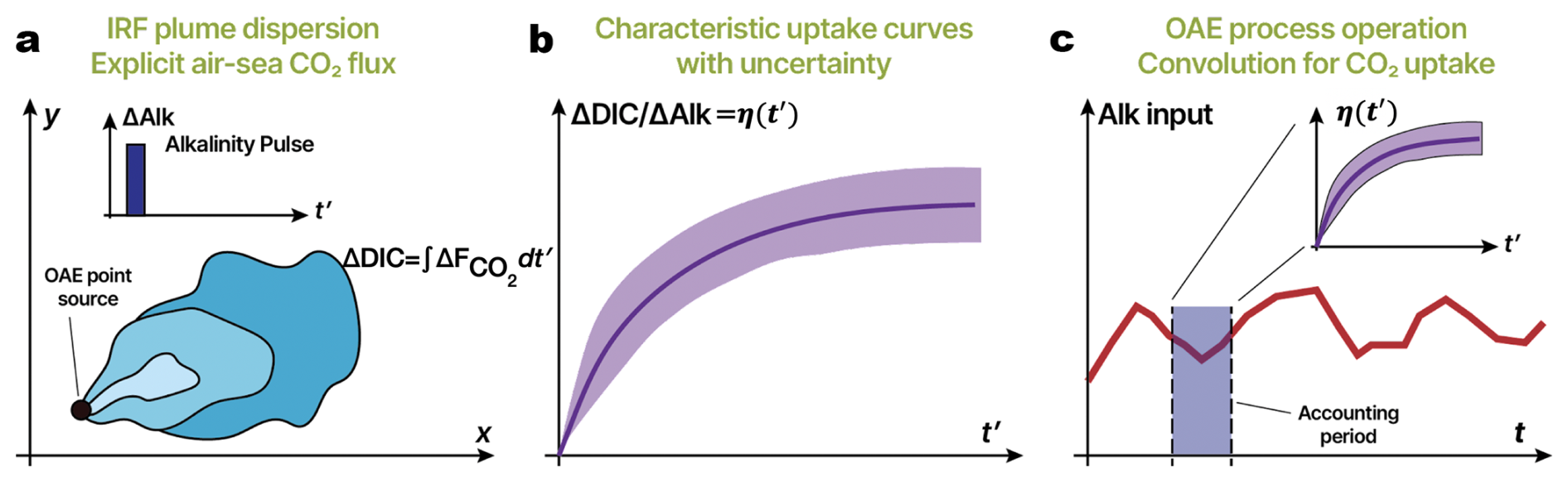
Figure 1 Overview of the IRF approach. (a) An alkalinity perturbation is applied as a pulse to the surface ocean from a point source; an alkalinity plume spreads (blue contours). There is an increase in DIC given by the integrated flux of carbon dioxide into the ocean from the OAE intervention ($\mathrm{\Delta }{F}_{{\mathrm{CO}}_{\mathrm{2}}}$). (b) The carbon uptake yields a characteristic uptake curve η. (c) If we now consider an arbitrary continuous release of alkalinity as a time series, a convolution of this forcing time series and characteristic uptake curve (IRF) may be performed to estimate the carbon uptake for accounting purposes. Note: t^′ is analogous to t and serves as a dummy integration variable.

Figure 1 provides an overview of the proposed IRF approach. An “impulse” of alkalinity forcing is applied as a pulse of a given ΔAlk at the surface from a point source. The alkalinity plume spreads over time. The OAE release has an associated characteristic uptake curve – η(t), which we call the “impulse response function” – with an envelope of uncertainty due to variability of the system that might be characterized by repeating the IRF experiment multiple times to sample differing winds, seasonal variability, mixing dynamics, biological activity, etc. If the system is sufficiently linear and time-invariant (detailed in the next section), we may perform a convolution of this uptake curve with any arbitrary alkalinity forcing to obtain the resultant uptake curve for that forcing. Figure 1c illustrates a continuous OAE deployment as a function of time. Computing carbon uptake owing to alkalinity released during the accounting period highlighted in purple would involve performing a convolution with alkalinity forcing over that time period and the characteristic curve shown in Fig. 1b.

2 Background on Impulse Response Functions

The application of IRFs to CDR quantification hinges upon two mathematical requirements: linearity and time invariance. Consider a system governed by a particular equation or set of equations, such as the ocean; an input, x, is supplied to the system, resulting in an output y. For mathematical purposes, x and y are arbitrary, but we can imagine x in our problem to be an alkalinity forcing x(t)=ΔAlk(t) and y to be the resultant carbon uptake efficiency curve y(t)=η(t). If we obtain an output y₁ for input x₁, and y₂ for input x₂, then the linearity condition states that for an input x₁+x₂ we will obtain an output y₁+y₂. A linear system should also obey homogeneity, such that for input ax₁+bx₂ we should obtain output ay₁+by₂. The second condition is time invariance. If we perturb our system with an impulse-like input (in practice, applied over a discrete but small time interval) at different points in time and obtain the corresponding impulse response functions, or outputs, h₁(t), h₂(t), h₃(t)…, these IRFs should be identical: $h_{\mathrm{1}}\left(t\right)=h_{\mathrm{2}}\left(t\right)=h_{\mathrm{3}}\left(t\right)\mathrm{\dots }$. In other words, the IRF is stationary in time. A system satisfying both of these conditions is known as linear and time invariant (LTI).

We make use of the Dirac delta function δ(t), which is a distribution that is zero everywhere except at the origin (t=0), with its integral over the entire real line being equal to 1:

$$\mathit{\delta }\left(t\right)=\left\{\begin{array}{ll}\mathrm{\infty },& t=\mathrm{0}\\ \mathrm{0},& t\ne \mathrm{0}\end{array}\right.$$

such that ${\int }_{-\mathrm{\infty }}^{\mathrm{\infty }}\mathit{\delta }\left(t\right)\mathrm{d}t=\mathrm{1}$. The idea of a convolution is to take an arbitrary signal x(t) and express it as a sum of simpler signals, i.e., a weighted sum of impulses. At t=0, we express x(t) as x(0) multiplied by the Dirac delta function, and likewise for all subsequent values of t (with appropriately shifted delta functions) so that:

$$\begin{array}{}\text{(2)}& x\left(t\right)=\underset{-\mathrm{\infty }}{\overset{\mathrm{\infty }}{\int }}x\left(t^{\prime }\right)\mathit{\delta }(t-t^{\prime })\mathrm{d}{t}^{\prime },\end{array}$$

where t^′ is a dummy variable for integration. Now, let us consider the output y(t) to an input x(t) of an LTI system. The IRF, denoted as h(t), is a known function describing how our system responds to an impulse. Extending the convolution idea, we rewrite our output y(t) as a weighted sum of impulse responses, so that:

$$\begin{array}{}\text{(3)}& y\left(t\right)=\underset{-\mathrm{\infty }}{\overset{\mathrm{\infty }}{\int }}x\left(t^{\prime }\right)h(t-t^{\prime })\mathrm{d}{t}^{\prime }=(x\ast h)\left(t\right).\end{array}$$

We have rewritten a complex function y(t) in terms of weights x(t) and impulse responses h(t). Note that linearity allows us to integrate over all the individual inputs, and time invariance allows us to conclude that if the response to δ(t) is h(t), then the response to δ(t−1) is h(t−1). For the OAE problem, we consider x to be an arbitrary alkalinity forcing, y to be the resulting carbon uptake efficiency, and h to be the uptake efficiency for an impulse-like alkalinity forcing, so that Eq. (3) becomes:

$$\begin{array}{}\text{(4)}& \mathit{\eta }\left(t\right)=\underset{-\mathrm{\infty }}{\overset{\mathrm{\infty }}{\int }}\mathrm{\Delta }\mathrm{Alk}\left(t^{\prime }\right)h(t-t^{\prime })\mathrm{d}{t}^{\prime }=(\mathrm{\Delta }\mathrm{Alk}\ast h)\left(t\right).\end{array}$$

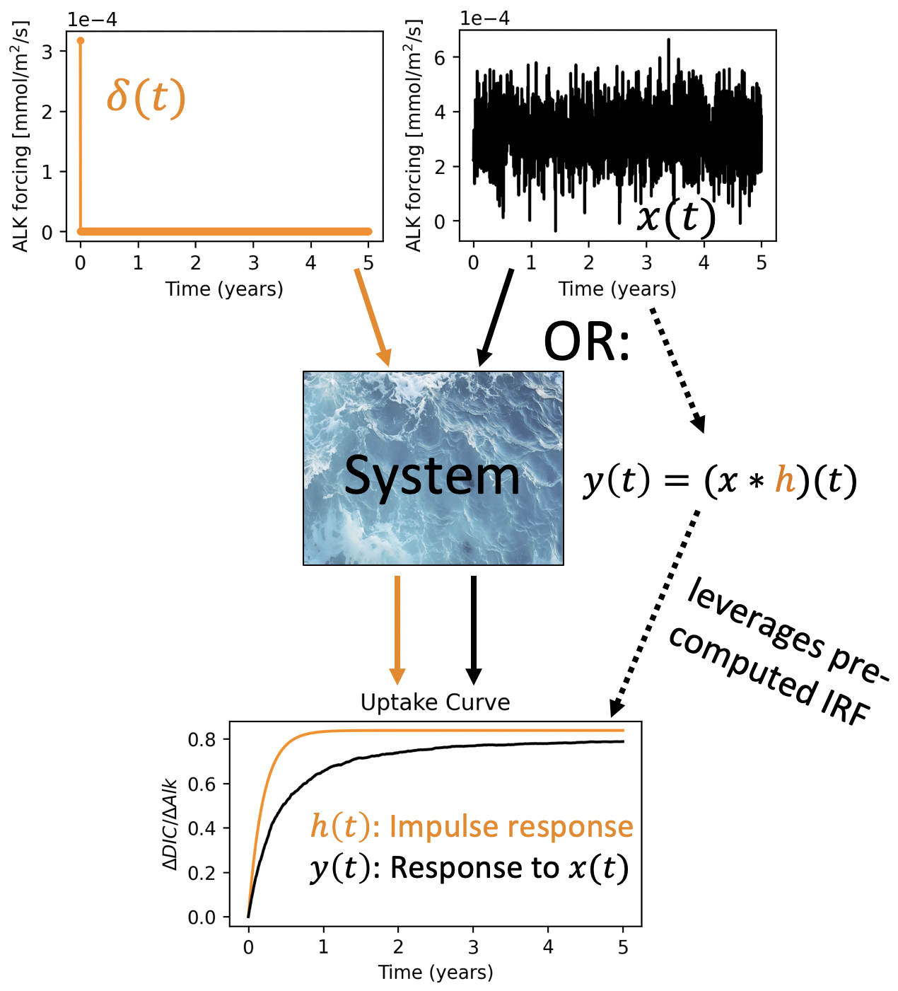
Figure 2 An illustration of why IRFs provide a powerful statistical and data reduction tool for the OAE problem. We consider our system to be the combination of chemical, biological, and physical processes influencing carbon uptake and distribution in the ocean. We probe the system by performing a model integration with a pulse δ(t) of alkalinity forcing and computing the resultant impulse response function h(t) defined as η(t) (OAE efficiency). Next, we want to obtain the OAE efficiency curve y(t) for a continuous five-year alkalinity deployment x(t). One option is to perform the full model integration for this OAE deployment and compute the resultant OAE efficiency. However, provided we have a sufficiently LTI system, we can compute the convolution of the IRF and the forcing, thus avoiding the need for an additional model integration.

One may ask: What is the advantage of rewriting y(t) or η(t) in the form of Eqs. (3)–(4)? As shown in Fig. 2, the IRF approach allows us to obtain the system's response y(t) for any arbitrary input x(t), provided that we know the IRF h and that the ocean is acceptably well-approximated as an LTI system. In other words, if we obtain the characteristic uptake curve(s) for an impulse of alkalinity forcing, we can then predict the uptake curve η(t) for any time series of alkalinity forcing ΔAlk(t). This is powerful because it implies that we no longer have to explicitly simulate the fate of every mole of alkalinity that we put into the ocean. We integrate the model to compute the IRF and then perform convolutions to predict the uptake for any alkalinity input. Of course, this simplification relies on staying within the bounds of LTI. Although we know that the ocean is not LTI, a major question that we address in this work is whether the statistics of the system are sufficiently stationary to allow us to apply the IRF approach via either a single IRF or library of IRFs encapsulating seasonal variability.

Several studies in the climate science field have successfully applied the IRF methodology to gain insight into various systems. Kuang (2010) used linear response functions to study deep cumulus cloud convection, which involves many nonlinear processes. Nonetheless, an ensemble can be used to create a reference state, and then linear response functions to small perturbations around this mean state were used to probe the dynamics of the cumulus ensemble and develop a parameterization. Joos et al. (2013) used IRFs to characterize the responses of metrics such as Global Warming Potential and Global Temperature Change Potential to emission pulses of CO₂ into the atmosphere. Hassanzadeh and Kuang (2016) used Green's functions (note that IRFs are a special kind of Green's functions with zero initial conditions) to determine the mean response of the climate system to weak forcing. They applied the response function alongside an eddy flux matrix to study eddy-mean flow interactions and gain insights into complex eddy feedbacks. All of these studies identify clear bounds under which the LTI assumption holds and the IRF approach is valid – doing so for the OAE problem is the subject of the next section.

3 Applying IRFs to the OAE Problem

Here we consider the chemical, physical, and biological controls on OAE uptake efficiency and implications for the LTI requirement. We begin by viewing the OAE problem as a purely chemical process neglecting oceanic dynamics, i.e., any processes that may advect, disperse, or subduct added alkalinity and thus modify the associated OAE efficiency curve. We then discuss the role of flow physics in modulating efficiency, the challenge of temporal variability, and the nonlinear dynamics arising from biological feedbacks.

3.1 Chemistry

From a chemical perspective, OAE operates by inducing a pCO₂ deficit at the surface ocean that is subsequently relaxed at a rate proportional to the gas exchange kinetics. The OAE efficiency η(t) may be expressed as a simple exponential (Zeebe and Wolf-Gladrow, 2001) as:

$$\begin{array}{}\text{(5)}& \mathit{\eta }\left(t\right)={\mathit{\eta }}_{max}(\mathrm{1}-e^{-t/\mathit{\tau }}).\end{array}$$

There are two parameters controlling the uptake efficiency. η_max is typically 0.7–0.9 depending on the background carbonate system. τ is the timescale of equilibration determined by gas exchange (Sarmiento and Gruber, 2006; He and Tyka, 2023) defined as:

$$\begin{array}{}\text{(6)}& \mathit{\tau }={\displaystyle \frac{\partial \mathrm{DIC}}{\partial \mathit{\text{p}}{\mathrm{CO}}_{\mathrm{2}}}}\cdot \left({\displaystyle \frac{z_{\mathrm{ML}}}{K_{\mathrm{0}}{k}_{\mathrm{w}}}}\right),\end{array}$$

where K₀ is the CO₂ solubility coefficient (Weiss, 1974), z_ML is mixed layer depth, k_w is the gas transfer velocity (Ho et al., 2006; Wanninkhof, 2014), and pCO₂ is the partial pressure of CO₂ (Sarmiento and Gruber, 2006). Typical values for τ range from 0.5 to 24 months, with a mean global value of 4.4 months (Jones et al., 2014). The linearity assumption states that the uptake curve η(t) should obey superposition – if two alkalinity pulses are applied independently, then η(t) should be the same as the case where the alkalinity pulses are applied together. This also means that both η_max and τ cannot be functions of ΔAlk. Otherwise, η(t) in Eq. (5) would nonlinearly depend on ΔAlk. We know this is not the case, but we aim to quantify the expected error and assess whether it is sufficiently small. We employ observed carbonate variables synthesized by the Global Ocean Data Analysis Project (GLODAPv2) (Lauvset et al., 2016; Olsen et al., 2016), to sample the full range of carbonate system conditions across the global surface ocean. We take the mean Alk and DIC state at every grid point and then apply perturbations to alkalinity (i.e., ΔAlk) ranging from 1 to 100 with intervals of 10 mmol m⁻³. For reference, the forcing employed in this study is $\mathrm{3.17}\cdot {\mathrm{10}}^{-\mathrm{4}}$ mmol m⁻² day⁻¹ (or 10 mol m⁻² yr⁻¹). We then analytically compute the corresponding η_max and τ as functions of temperature, salinity, phosphate, silicate, Alk, and DIC based on the governing equations of the carbonate system (Sarmiento and Gruber, 2006). The calculation involves solving for the re-equilibrated DIC following a ΔAlk addition and assumes a constant atmospheric pCO₂ of 425 ppm. The difference in re-equilibriated and initial DIC divided by ΔAlk yields η_max. We ask whether η_max and τ change substantially as the alkalinity perturbation increases.

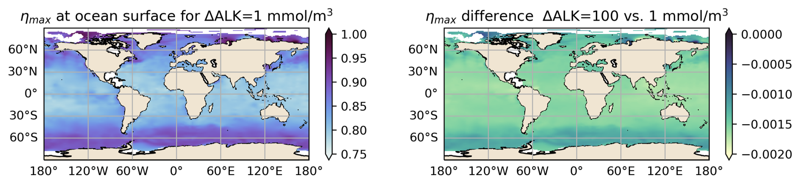
Figure 3 Left: values of the maximum theoretical OAE efficiency η_max for the global ocean based on climatological GLODAPv2 observations (Lauvset et al., 2016; Olsen et al., 2016) for a ΔAlk perturbation of 1 mmol m⁻³. Right: the difference in η_max for ΔAlk of 100 and 1 mmol m⁻³. Note: these calculations assume an idealized, non-interactive atmosphere.

We first test the linearity condition for η_max in Fig. 3. We note that the maximum theoretical OAE efficiency varies from 0.75 at low latitudes to 0.9 at high latitudes. Looking at the difference between the ΔAlk=100 and 1 mmol m⁻³ cases, there appears to be only a slight decrease in η_max as the forcing increases. To compare more quantitatively, we create a parameter space of DIC and Alk based on surface climatology and compute the η_max for each value of the ΔAlk perturbation. We compute the slope of the resulting curve to obtain the change in η_max per mmol m⁻³ of added Alk. The result is plotted in the left panel of Fig. 4. The percent change in η_max for 100 mmol m⁻³ of added Alk is less than 0.1 %, nearly negligible for the entire parameter space considered here. Given the expected magnitudes of Alk perturbations induced by CDR deployments, it is unlikely that we will introduce alkalinity perturbations in excess of 100 mmol m⁻³ at the CO₂ equilibration scales following dilution and spread of the alkalinity plume (though possible in the vicinity of the OAE deployment). η_max is essentially unaffected for such a perturbation. Thus, we conclude that η_max does not present significant nonlinearity. We then consider a similar test for the gas exchange timescale, τ. We assume that K₀, z_ML, and k_w are not functions of alkalinity, and thus the nonlinearity may be encapsulated by a parameter κ:

$$\begin{array}{}\text{(7)}& \mathit{\kappa }={\displaystyle \frac{\partial \mathrm{DIC}}{\partial \mathit{\text{p}}{\mathrm{CO}}_{\mathrm{2}}}}.\end{array}$$

In the right panel of Fig. 4 we compute the rate of change in κ per mmol m⁻³ of added Alk between ΔAlk=1 and 100 mmol m⁻³. We note that κ, and thus τ, is more sensitive to the magnitude of the alkalinity perturbation than η_max was, increasing up to 65 % for a 100 mmol m⁻³ Alk perturbation. Still, for the forcing values considered here we expect τ to increase by at most only a few percent, not significantly hindering the IRF linearity requirement (though this will be assessed in the results).

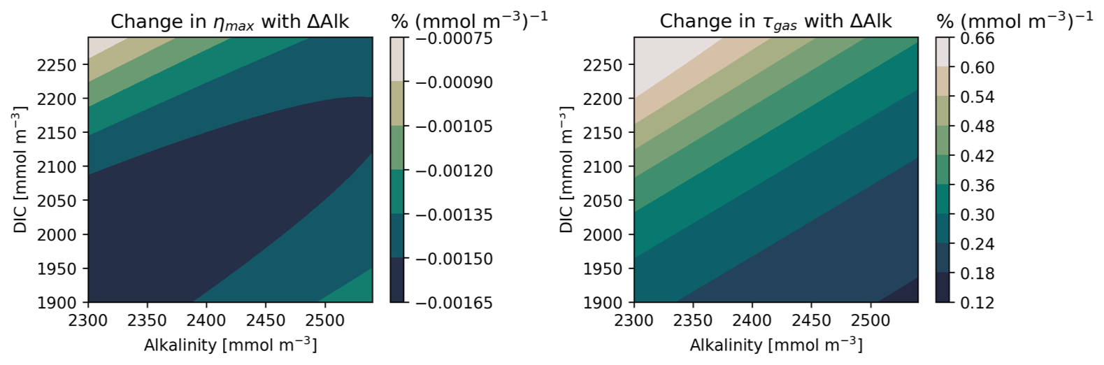
Figure 4 We assess how the efficiency η_max and carbon uptake timescale τ change with the magnitude of the alkalinity perturbation ΔAlk. We compute η_max and κ (Eq. 7) for in situ oceanic DIC and Alk values taken from the GLODAPv2 dataset and perturbations ΔAlk=1 to 100 mmol m⁻³ with intervals of 10 mmol m⁻³. We find the linearized rate of change of η_max and κ relative to ΔAlk. We may thus obtain the percent change in η_max (left) and τ (right) per mmol m⁻³ of alkalinity added.

We acknowledge other potential sources of chemical nonlinearity may arise when considering the “additionality problem” (Bach, 2024). The climatic benefit of OAE may be defined by its additionality, or how much the OAE intervention increases CO₂ removal relative to a baseline state without OAE. However, OAE may also modify the natural alkalinity cycle and associated baseline calcium carbonate saturation state, leading to changes in biogenic calcification. The study by Bach (2024) presents experiments showing that OAE can reduce the generation of natural alkalinity, thereby reducing additionality in many of the marine systems where OAE is being considered. The additionality problem is enhanced in natural alkalinity cycling hotspots, such as marine sediments. Regarding time invariance, the carbonate chemistry equations are invariant by formulation. The only place where time invariance may be violated in the above equations is in k_w. Since k_w is determined by wind speed, and thus the dynamical ocean/atmosphere component, we return to it in the next section on physics. Thus, from a purely chemical perspective, we have shown that the LTI requirement is a reasonable approximation.

3.2 Physics and Time Invariance

The physical equations governing the ocean and atmosphere system are not, to first order, functions of alkalinity, and we assume that the ΔAlk perturbation magnitude will have a negligible influence on resulting dynamics for at least the decadal timescale following the OAE intervention. A caveat is that in our numerical simulations we assume a non-responsive atmosphere; i.e., the change in the atmospheric CO₂ reservoir is negligible. Although OAE will decrease the atmospheric CO₂ and thus impact CO₂ uptake, for small OAE deployments we can accurately capture the first-order carbon uptake curve by assuming a non-interactive atmosphere, making modeling more affordable (Tyka, 2024). We assume that the linearity condition is sufficiently satisfied from a physical perspective. However, the time invariance condition poses ambiguity as to whether and how we may successfully apply IRFs for MRV. Particularly for an OAE deployment occurring over a small spatiotemporal scale, the uptake curve may be significantly affected by local tidal flows, turbulence and mixing patterns, and the seasonal and interannual flow variability characterizing the particular time and place of interest. Weather patterns and resulting wind dynamics also strongly influence air-sea gas exchange, as k_w in Eq. (6) depends on the average square of 10 m height neutral winds (Ho et al., 2006; Wanninkhof, 2014). Similarly to physical subduction, wind speed variability may lead to drastically different carbon uptake curves and violate time invariance. We employ two strategies to deal with these challenges posed by ocean and atmosphere variability. First, for our IRF experiments we use alkalinity pulses that extend for a one-month duration and span several hundred square kilometers, sufficient to integrate over dominant periodicities in local flows (e.g. tides or eddy features). Additionally, we generate libraries of IRFs capturing seasonality and perform ensembles to estimate the uncertainty associated with interannual variability. Nonetheless, due to the complexity and nonlinearity of the ocean-atmosphere system, it is challenging to say a priori how this will project onto our ability to utilize IRFs for CDR quantification successfully.

3.3 Biology

The biological system of the ocean poses a challenge to the LTI requirement due to its inherent complexity and potential for feedbacks. Bach et al. (2019) provides a survey of knowledge gaps and hypotheses regarding how different chemical forms of OAE may impact the biological system. For example, in OAE interventions employing quicklime (CaO), calcifying organisms are expected to benefit. On the contrary, when using olivine, silicifiers and cyanobacteria are expected to increase primary productivity significantly. Either scenario may lead to changes in the biological carbon pump. Suessle et al. (2025) discuss how the vertical fluxes of carbon, nitrogen, phosphorus, and silicon may be affected by perturbation magnitudes of alkalinity. An encouraging result of their work is that carbon export by oligotrophic plankton communities is insensitive to OAE perturbations (though they suggest additional investigation in less idealized models). In the last year, numerous studies have probed the influences of various marine-based CDR approaches on biological and carbon cycle feedbacks. For example, Berger et al. (2023) found that when macronutrient limitations and biological feedbacks are parameterized in their model, the efficiency of macroalgae-based CDR drops. Other studies have considered OAE effects on coastal fish larvae (Goldenberg et al., 2024), diatom silicification (Ferderer et al., 2024) and phytoplankton responses (Xin et al., 2024; Hutchins et al., 2023). We conclude that assessing a priori the magnitude of nonlinearity and time invariance of the biological system to perturbations in ΔAlk is beyond the scope of this work. We acknowledge the potential for biological feedbacks and the importance of considering and quantifying such phenomena. In the near term, however, we expect OAE signals to be small except in the local area immediately adjacent to perturbations (the near-field). We envision an approach employing observations and high-resolution models to quantify the near-field dynamics, including various feedback elements, and subsequently hand off these results to an IRF-based approach at larger scales where signals are more diffuse.

4 Numerical Experiments

Having presented the IRF framework and the physical, chemical, and biological system constraints to applying IRFs in the real ocean, we move towards applying IRFs for quantifying OAE-based CDR in a global climate model. The objective is to first obtain an IRF (or a “library” of IRFs accounting for seasonal variability) and then use it to predict the uptake curve of a continuous alkalinity deployment. We will assess the accuracy with which the IRF prediction can reproduce the actual continuous release model simulation, and consider several distinct dynamical and biogeochemical regimes in the ocean.

Our study followed the experimental design outlined in Zhou et al. (2025), hereafter referred to as Z25. Z25 employed the Community Earth System Model version 2, CESM2 (Danabasoglu et al., 2020), in the forced ocean-ice configuration, FOSI (Yeager et al., 2022). The ocean component of the model is the Parallel Ocean Program version 2 (POP2), integrated at a 1° horizontal resolution and forced by the Japanese 55-year atmospheric reanalysis dataset, JRA55 (Kobayashi et al., 2015). The forcing includes the historical transient in atmospheric CO₂, and the model was integrated using repeating JRA55 forcing cycles from 1850 to near-present, thus accounting for the accumulation of anthropogenic CO₂ in the ocean. POP2 is coupled to the Marine Biogeochemistry Library, MARBL (Long et al., 2021). MARBL simulates two carbonate systems in parallel online; thus, the baseline and the case with the OAE intervention are computed simultaneously within a single model integration. The Z25 study divided the Global Ocean into 690 polygons and performed separate global model integrations for OAE deployments within each polygon. Alkalinity was released at the polygon's surface at a constant rate of 10 mol m⁻² yr⁻¹ for one month (sufficiently short to resolve seasonal and interannual variability), and the model was integrated for 15 years post-release. As discussed in Z25 and He and Tyka (2023), such a flux magnitude generally ensures that: (1) the pH increase is less than 0.1, which is the amount that pH has already decreased in the surface ocean since preindustrial times (Doney et al., 2009), and (2) the aragonite saturation state change is less than 0.5, preventing the secondary precipitation of calcium carbonate which would decrease OAE efficiency (Moras et al., 2022). To investigate the seasonal variations of OAE efficiency, four separate simulations were performed for each polygon with alkalinity releases in January, April, July, and October 1999. Thus, Z25 provides the first geographically-refined global map of OAE efficiency with an assessment of seasonal variability. For additional details on the experimental design, model details, and discussion of global variations in OAE efficiency, please refer to Z25 (Zhou et al., 2025).

In our work, we treated the simulations of Z25 as the “impulse” experiments, and the seasonal Z25 uptake curves as our “IRF library”. We chose 9 polygons in the North Atlantic, and 8 polygons in the North Pacific, with various efficiencies and seasonal variability. We then performed continuous OAE release experiments beginning in 1999 and lasting five years, with the same magnitude of forcing as in Z25. For select polygons, we also performed a one-year continuous release experiment. We computed a convolution of our prescribed forcing with the Z25 seasonal IRF library to get an IRF-based prediction of the carbon uptake efficiency as a function of time for the continuous release simulations. We then compared the explicitly-simulated and predicted efficiency curves to assess the validity of the IRF approach. To quantify the uncertainty associated with interannual variability, we additionally performed ensemble simulations for a selection of the polygons we considered. The ensembles consist of separate one-month alkalinity deployments (identical to Z25) in January of 16 years, ranging from 1999 to 2014. Examining the spread in uptake efficiency curves across these 16 January OAE deployments provides insight into the expected uncertainty of the IRF prediction (which is based on just one year) for a given polygon.

5 Results

Here, we go through the procedure for applying the IRF-based CDR quantification to the OAE problem. We will begin by discussing the spatiotemporal scales of the OAE problem, discuss seasonal and interannual variability and its influences on the IRF approach and resultant uncertainty, and end by showing a synthesis evaluating the performance of the IRF prediction across different ocean basins and dynamical regimes.

5.1 Spatiotemporal Scales

As stated above, the first step is to obtain the IRF library for a given polygon from Z25; Fig. 5 presents one example for the coast of southern California. The excess alkalinity at the surface is seen to spread through the entire zonal extent of the Pacific by about 10 years. By 15 years, most of the surface of the Pacific within 40° of the equator has excess alkalinity associated with the intervention.

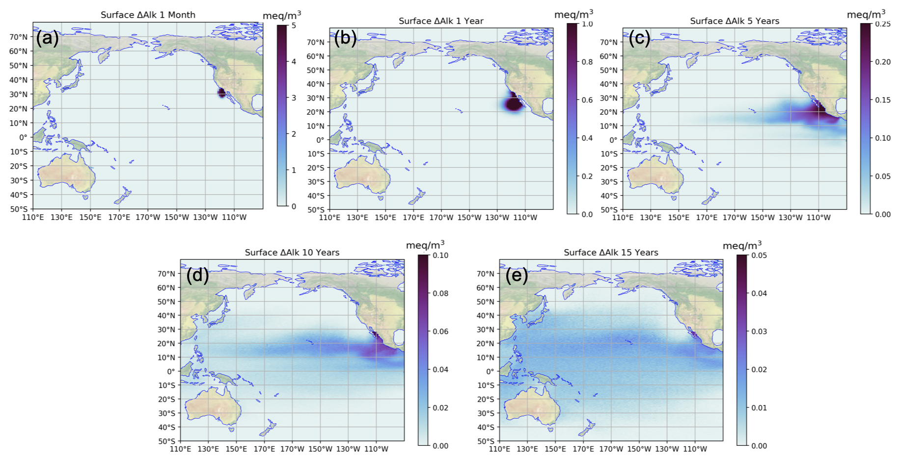
Figure 5 Evolution of excess alkalinity at the surface following the month-long January alkalinity release off the coast of California, see Polygon 214 in Fig. 12. Times post-release are 1 month, 1 year, 5 years, 10 years, and 15 years (a–e, respectively).

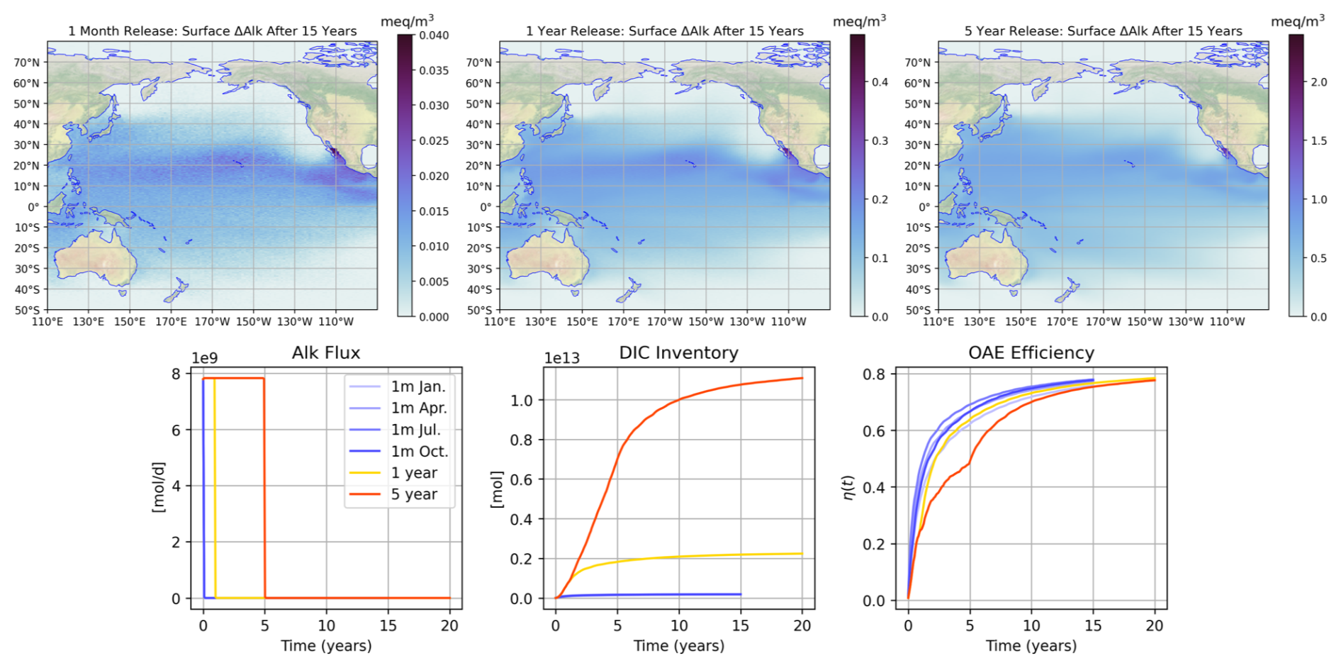
Figure 6 Overview of the simulations used to test the IRF approach at the southern California location (Polygon 214 in Fig. 12). The top row shows the excess alkalinity at the surface for the month-long January OAE simulation 15 years post-release, the 1-year continuous release 15 years post-release (16 years since the beginning of the model integration), and the 5-year continuous release also 15 years post-release. The colorbars are adjusted for the latter two based on the total amount of alkalinity released so that they are directly comparable to the first plot in terms of color. One can thus observe that the surface alkalinity distributions between these cases are nearly identical. The bottom row shows the alkalinity forcing time series for the four separate month-long and two continuous release cases, the excess DIC inventory as a function of time, and the OAE efficiency (η) as a function of time for each case.

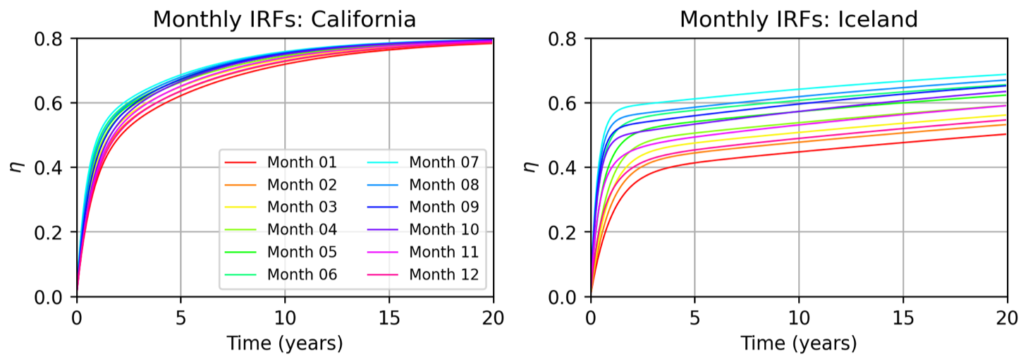
Figure 7 Using the month-long alkalinity release simulations conducted in January, April, July, and October by Zhou et al. (2025), we construct a library of IRFs for each location corresponding to each month by linearly interpolating between months 1, 4, 7, and 10. The left panel shows the resulting monthly IRFs for California (Polygon 214, Fig. 12), and the right panel is Iceland (Polygon 36).

In Fig. 6 we show the distribution of excess alkalinity at the surface for the January “impulse” simulation as well as our two continuous release cases, 15 years post-release. One can see that the surface alkalinity distribution, when normalized by the total amount of alkalinity added (accomplished by scaling the colorbar), appears to have the same distribution for all cases. The lower left panel of Fig. 6 shows the time series of alkalinity forcing – note that alkalinity flux is the same 10 mol m⁻² yr⁻² for the month-long and continuous releases. The middle panel shows the net change in DIC inventory for each case, and the last panel shows the curves of OAE efficiency η for each case. Note that the blue curves are our “IRFs” since they represent the response of the system to an alkalinity forcing impulse. The continuous-release simulations have different uptake curves; the kinks in the curve represent the cessation of alkalinity addition. Net ΔAlk (denominator of η) increases as alkalinity is added, causing a flatter curve. The kink is most obvious in the 5-year release.

5.2 Seasonality

As discussed, our IRF metric is efficiency η(t). Z25 provides us with seasonal IRFs, but a few details should be noted regarding their implementation. Since the IRFs end at 15 years, we fit an exponential curve to them so that we have an analytical form for the IRF that we may extend longer in time. The exponential has the form:

$$\begin{array}{}\text{(8)}& \begin{array}{rl}h\left(t\right)& =\mathit{\eta }\left(t\right)={\mathit{\eta }}_{max}\left[\mathrm{1}-\mathit{\alpha }{e}^{-t\left(\frac{\mathrm{1}}{{\mathit{\tau }}_{\mathrm{1}}}+\frac{\mathrm{1}}{{\mathit{\tau }}_{\mathrm{2}}}\right)}-(\mathrm{1}-\mathit{\alpha })e^{-\frac{t}{{\mathit{\tau }}_{\mathrm{3}}}}\right],\\ & \mathrm{with}\mathit{\alpha }={\displaystyle \frac{{\mathit{\tau }}_{\mathrm{2}}}{{\mathit{\tau }}_{\mathrm{1}}+{\mathit{\tau }}_{\mathrm{3}}}}.\end{array}\end{array}$$

In Eq. (8), τ₁, τ₂, and τ₃ are adjustment timescales over which the CO₂ equilibration occurs; τ₁ is the fast adjustment driven by gas exchange, τ₂ is the longer-term adjustment, and τ₃ represents the transition from τ₁ to τ₂. The three timescales and η_max are the free parameters which are solved for using a curve fitting algorithm for each of the seasonal IRF experiments. η_max is initialized with an average climatological value but adjusted as the curve fitting iterations progress. We found this analytical form to reconstruct the IRF data successfully; for more details on curve fitting methods see supplementary information of Zhou et al. (2025). We could just as readily use the η(t) curves themselves without performing the fitting, but to decrease the data volume and allow for longer time series in our convolutions, we opted for the curve-fitting route. The next detail is how to apply the IRFs to perform the convolution with forcing and obtain an IRF-based carbon uptake prediction. Since our two continuous release simulations both begin in January, our first approach is simply to take the January IRF and proceed. However, Z25 identified many regions as having strong seasonality, thus violating the time invariance condition. In Fig. 7, we perform a linear interpolation of the January, April, July, and October 1999 IRFs to get a monthly IRF library. We show the resulting IRFs for the California location considered in Figs. 5–6. Note that at this location, all IRFs are relatively close together, i.e., seasonality is weak, and time invariance is not violated significantly. However, considering the same plot for the Iceland OAE location, we notice up to a 50 % increase in efficiency between the winter and summer months (Fig. 7).

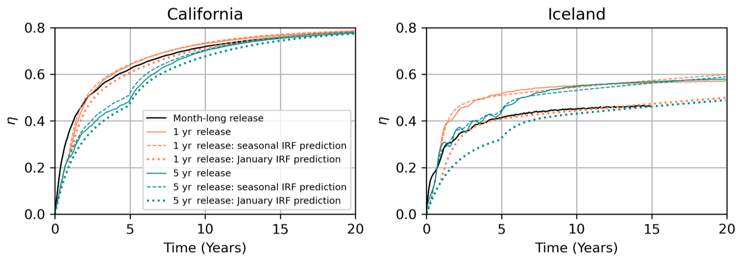
Figure 8 Comparison of the IRF prediction and model integration result for the continuous release simulations in California (left) and Iceland (right), Polygons 214 and 36 in Fig. 12. The black line shows the OAE efficiency (η) curve for the month-long January release. The solid orange and dark cyan lines are the OAE curves obtained from the model integration of a 1 and 5-year continuous alkalinity release experiment, respectively. The dashed line shows the corresponding prediction using IRFs constructed for each month as shown in Fig. 7. The dotted line is the prediction using only the January IRF, without constructing an individual IRF for each month to account for seasonal variability.

Our first approach is to simply take the January IRF and perform the convolution with a time series of 1 and 5-year continuous alkalinity forcing to obtain the resulting IRF predictions, $\mathit{\eta }(t{)}_{\mathrm{1}\mathrm{yr},\mathrm{5}\mathrm{yr}}=(\mathrm{\Delta }\mathrm{Alk}\ast {\mathit{\eta }}_{\mathrm{Jan}}\left)\right(t)$. We compare the actual and predicted η(t) for the continuous release simulations in Fig. 8. For the California location, the January IRF prediction performs well and aligns with the η(t) curves for both continuous-release simulations. The greatest deviation occurs in years 2–5 and is attributable to interannual variability, but after a few years, the predicted and actual curves converge. However, this is not the case for Iceland. We see a significant underestimation of about 20 % by the IRF compared to the model result. This is because we have violated time invariance and are using the January IRF, which does not encapsulate the summer behavior at this location. So, instead, we perform the convolution month-by-month using the monthly IRFs from Fig. 7. Note that at the Iceland location, using the monthly IRFs substantially improves the IRF prediction, so it is nearly aligned with the actual model result. Interestingly, at the California location, the seasonal and January IRFs have roughly the same deviation from the actual curve. This indicates that the interannual and seasonal variability have similar magnitudes, whereas in Iceland, the seasonal variability substantially dominates in magnitude.

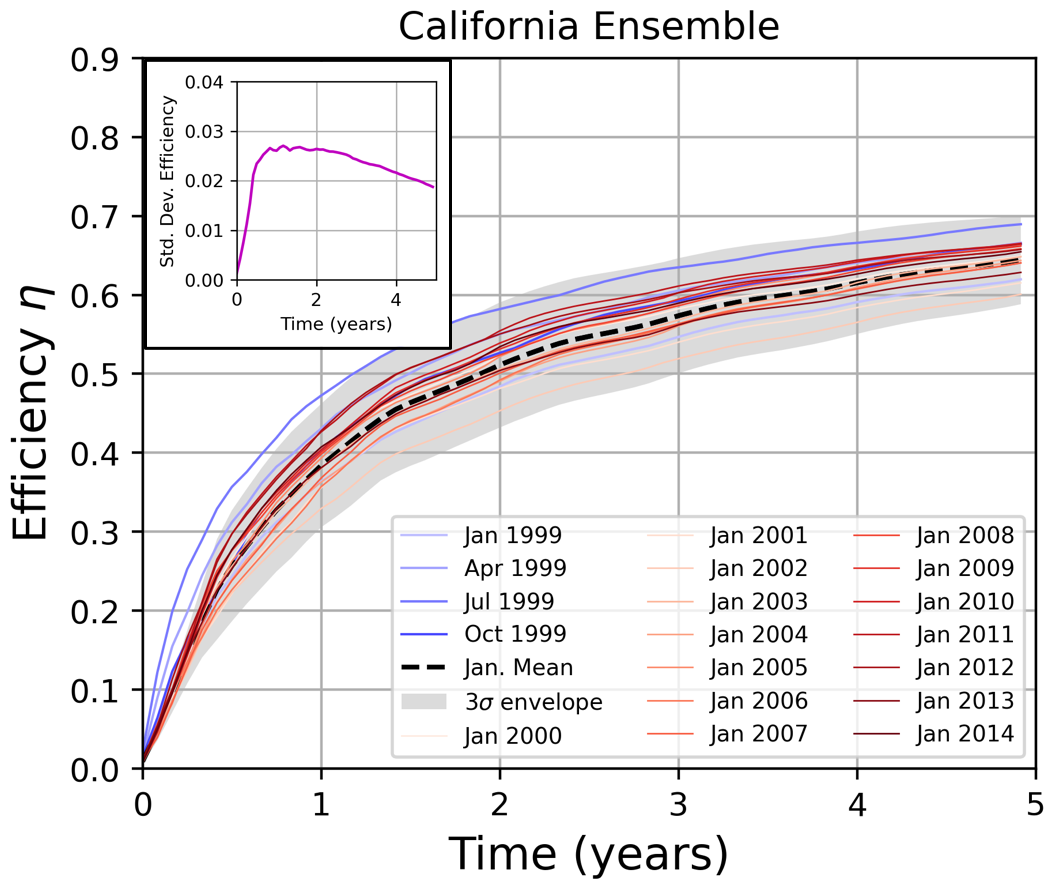
Figure 9 Ensemble results of efficiency η for the California location (Polygon 214, Fig. 12). We conduct a series of 16 model integrations beginning in each year from 1999 to 2014, with a month-long release of alkalinity in January of each starting year. These results are shown as red lines, and their mean is shown as a dashed black line. In gray is the envelope encompassing three standard deviations from the mean; in blue are the four seasonal simulations of month-long OAE deployments in January, April, July, and October of 1999. This figure allows one to compare the seasonal variability in η to the interannual variability. The insert shows the standard deviation in η of the January releases at this location as a function of time. Analogous plots for other locations are shown in Fig. 11.

5.3 Interannual variability

To gain deeper insight into the variability – particularly to test our statement above that seasonal and interannual variability are comparable at the California location – we performed ensemble simulations detailed in Sect. 4. This is illustrated in Fig. 9 for the California location. One can immediately observe that there is variation in January uptake curves depending on the year. Interestingly, the standard deviation of the ensemble members peaks between 1–2 years and then decreases. This explains why in Fig. 8, the 1999-based IRF prediction deviates slightly from the explicit simulation in the several years following the OAE deployment and then converges to the model result. We have shown that the IRF-based CDR quantification is valid once the time variance of the IRF is accounted for at two sample locations – California and Iceland. We now test the approach of applying the monthly IRFs capturing seasonal variability at four other locations with differing dynamical regimes and uptake curves. These regions are: the Labrador Sea, North Sea, Western Equatorial Pacific, and North Pacific (see Polygons 0, 16, 334, and 305, respectively in Fig. 12). As in the prior section, we first compute a monthly IRF for each location by fitting an exponential curve to the four seasonal IRFs from Z25 and linearly interpolating between the months. We compute the convolution of IRF and alkalinity forcing month-by-month for our 1 and 5-year continuous alkalinity forcing cases. We perform model integrations for the continuous OAE releases and compare the resulting uptake with our IRF prediction. Finally, we perform ensembles consisting of 16 members. Each member simulates a month-long January alkalinity release in a year ranging from 1999–2014, and is integrated for five years post-release.

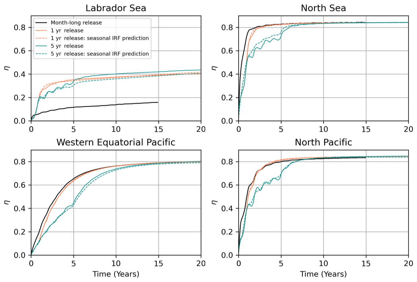
Figure 10 Comparison of the IRF prediction and model integration results for the continuous release simulations in the Labrador Sea (Polygon 0, Fig. 12), North Sea (Polygon 16), the western equatorial Pacific (Polygon 334), and north Pacific (Polygon 305). The black line shows the OAE efficiency (η) curve for the month-long January release. The solid orange and dark cyan lines are the OAE curves obtained from the model integration of a 1 and 5-year continuous alkalinity release experiment, respectively. The dashed line shows the corresponding prediction using IRFs constructed for each month.

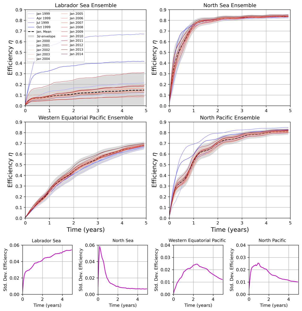
Figure 11 Ensemble results of efficiency η for the same locations as Fig. 10. Month-long January releases from 1999 to 2014 are shown as red lines and the mean is shown as a dashed black line. We also show the envelope encompassing three standard deviations from the mean, as well as the four seasonal simulations of month-long OAE deployments in 1999 (blue lines). The lowest row shows the standard deviation in η of the January releases as a function of time.

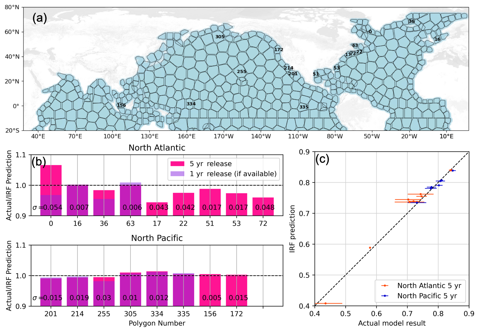
Figure 12 (a) Polygons defined by Zhou et al. (2025), with the ones considered in this study for testing the IRF approach labeled in black. (b) Bar charts show the ratio of the modeled continuous release compared to the IRF prediction 15 years after the end of the alkalinity release. Dark pink is the 5-year continuous release case, and violet (semi-transparent) is the 1-year continuous release case. The numbers on the bars indicate the standard deviation after 5 years of ensembles performed for a given polygon. Note that not all polygons have an ensemble result, and not all polygons have a 1-year result (due to computing constraints). (c) Similar to (b), here we present the IRF prediction vs. the actual model result for the 5-year release cases, with the one-to-one line shown as a black dashed line. Error bars show the standard deviation from the ensemble results.

The results for these four locations are shown in Fig. 10. We first note that the IRF prediction matches nearly perfectly with the 1-year release simulation at all four locations. This agreement stems from the fact that the monthly IRFs used in this prediction were taken from the year the alkalinity was released, so we mostly account for the effects of seasonal variability – and interannual variability is not a factor. However, for the 5-year case, we are still using the 1999 IRF, even though alkalinity continued to be released from 1999–2004. As a result, the IRF does not capture the effects of interannual variability. Nonetheless, we see remarkable agreement between the IRF and model results in all regions except the Labrador Sea (where there is roughly a 10 % error). In the North Sea, interannual variability becomes important 2–6 years into the simulation, and the IRF diverges from the model result. However, over time, the ensemble spread decreases (variability averages out), and the IRF curve converges with the explicit simulation results after 7 years. Similar, though slightly smaller trends, are also apparent in the Pacific cases. The interannual variability is shown in Fig. 11. For the Labrador Sea, the model simulates a large interannual variability that explains the error in the IRF prediction. At this location, strong wintertime convection removes the alkalinity from the surface and leads to very low values of η. The magnitude of this convection is highly variable year-to-year. We note that the year 1999, for which our IRFs were constructed, had particularly strong convection and a lower-than-average efficiency – this is why the IRF prediction in Fig. 10 underestimated the actual curve. Furthermore, the standard deviation of the ensemble members increases as a function of time, so the IRF and model results do not converge with time, implying that convection removes alkalinity from the surface for longer timescales than the 10–20 years we consider. Interestingly, at the three other locations, the ensemble standard deviation peaks and then decreases. Again, this explains why the IRF predictions that initially deviated from the model result eventually converged. Interestingly, despite the interannual variability often being similar in magnitude to seasonal variability, and our IRFs not taking into account the interannual variance, we still obtain an excellent matchup with the model results.

5.4 Comparison across regions

In Fig. 12 we synthesize all of the results for the polygons considered in this study. Note that the 1-year continuous release case is less “challenging” for the IRF approach as our IRFs were also constructed from 1999 impulse experiments. The 5-year case faces the time invariance problem, since we add alkalinity to years other than 1999 but still use the 1999 IRFs. Remarkably, in all cases, the error of the IRF approach is less than 7 %, even in the highly variable Labrador Sea. In the Pacific, the errors are even smaller, within 1 % of the model result. One can see that the higher errors stem from the higher interannual variability (violating the LTI requirement). The 1:1 line in panel (c) shows where the IRF prediction matches the model result, and nearly all points with the associated error bars fall onto this line. We conclude that once an appropriate seasonally-varying IRF is constructed, the IRF approach may be applied to successfully predict the carbon uptake associated with an OAE deployment without the need to perform a model integration explicitly. We are able to stay within sufficient bounds of linearity and time invariance required for the IRF approach to work.

We note the potential of creating IRF libraries over the historical period to account for interannual variability (for instance, ENSO). An interesting question to consider is when should a given IRF be recomputed, or how accurate is an IRF years later? Here we can only speculate, given that our simulations ran for a maximum of 20 years. In certain regions interannual variations are substantial and the IRF approach leads to high errors even with a 5-year old IRF. Other regions exhibit smaller interannual variability over years-decades. The frequency with which IRFs need to be recomputed will vary depending on the variability of the region under consideration and the model used to compute the IRFs. We hypothesize that the relatively laminar 1° CESM exhibits less turbulence and flow variability than a higher-resolution model. Promisingly, the standard deviation in ensemble members decreases over time in most regions. Based on our results, using a seasonal IRF library from one year and then performing an alkalinity release for 5–10 years afterwards will lead to a reasonable prediction in most regions.

6 Discussion and Conclusions

We have presented compelling results indicating that impulse response functions (IRFs) may be a powerful tool in aiding the Monitoring, Reporting, and Verification (MRV) of ocean alkalinity enhancement (OAE) interventions. The premise is that we can probe the complex ocean, terrestrial, biological, and atmospheric system by forcing it with an “impulse” – a short pulse of alkalinity applied to the surface ocean. By constructing an OAE efficiency curve for the resultant carbon uptake from our intervention, we can predict the carbon uptake for any arbitrary time series of alkalinity forcing, provided we have a linear and time invariant (LTI) system. We first discussed and quantified the sources of nonlinearity and time invariance in the system. We then tested the IRF approach in the CESM 1° resolution global climate model. For our impulse simulations, we used the OAE Efficiency Atlas created by Zhou et al. (2025) (Z25). We performed continuous alkalinity release simulations, and found remarkable agreement between the IRF prediction and model results. In most regions, the IRF prediction is typically within 1 % of the actual model result. We determined the accuracy of the IRF to hinge predominantly on the magnitude of the interannual variability at the given location; we quantified this by performing 16-member ensembles.

Though this study has shown great potential for future use of IRFs for MRV of ocean alkalinity enhancement interventions, many additional questions have come up. The biggest challenge in assessing OAE influences is its multiscale nature, which is highly sensitive to the various modes of variability comprising the Earth system. The global model used here has a horizontal resolution of 1° (≈ 100 km). This resolution cannot resolve oceanic mesoscale features, such as eddies, certain coastal processes, or submesoscale dynamics such as fronts, filaments, mixed layer eddies, and inertial-symmetric instabilities. These smaller scale dynamics may lead to or inhibit vertical transport of alkalinity that could be highly relevant to setting the OAE efficiency. There is also the question of how realistic our initial condition and forcing scenario are. Our polygons were all on the order of several hundred kilometers in length and width and experienced constant alkalinity forcing over that area with a relatively small flux of 10 mol m⁻² yr⁻¹. In practice, alkalinity will be released from point sources, and tracing its progression from the order of a few meters to the size of the polygons represents a large technical challenge. Due to the multiscale nature, there is no numerical framework capable of resolving all of the relevant spatiotemporal scales and multi-scale coupling is prohibitively computationally expensive.

Constraining the small-scale turbulence and mixing influencing the near-field and short-term evolution of an alkalinity plume and coupling this to the larger-scale dynamics remains an important avenue for future work. We envision using the IRF for tracing the evolution of the OAE intervention at the larger, gas-exchange scales. Linking the high-resolution near-field modeling/observations to the coarser-resolution regional/global scale modeling remains a critical component to successful MRV of OAE. Additionally, exploring what length of “impulse” is appropriate (here we only considered one month) may be an interesting question to pursue when considering various modes of oceanic variability. In our coarse global model, the month-long pulses were sufficiently short compared to the characteristic seasonal variability. As a result, we constructed a library of IRFs sampling over this variability. If we consider high-resolution simulations of a tidally-driven estuary, for example, an hour-long pulse would preference a particular tidal phase, and we would similarly need to construct a library of IRFs sampling the tidal cycle. Or, we could envision a longer deployment of 12–24 h to sample over the full tidal cycle.

Another assumption in our work is that of non-interactive atmosphere and terrestrial components. Although generally considered second-order effects for the purpose of carbon accounting (Tyka, 2024), interactive atmosphere and terrestrial carbon pools may be important future considerations. An interactive atmosphere decreases the sensitivity of the biological pump to changes in carbon uptake, and including the terrestrial component increases the fertilization-induced marine carbon uptake Oschlies (2009). Exploring a more realistic interaction of the ocean, atmosphere, and land systems is an important future step in understanding OAE influences in projecting onto the global carbon budget (Friedlingstein et al., 2023). We acknowledge the limitations arising from using one modeling framework with its particular set of assumptions and biases – nonetheless, our results are an encouraging proof-of-concept that may now be extended to other modeling efforts and inter-comparison projects.

The next steps in this work involve closing the gap between the laminar dynamics of the order 100 km grid model used in this study and the meter-to-kilometer scale dynamics potentially relevant for MRV of OAE interventions. We are applying the results of this work to guide further regional modeling efforts aimed at resolving mesoscale turbulence, and potentially some submesoscale dynamics. We anticipate future work applying the Regional Ocean Modeling System (ROMS) (Shchepetkin and McWilliams, 2005) to perform high-resolution regional simulations analogous to the CESM simulations presented here. Regional simulations will allow us to study the role of smaller-scale ocean dynamics in modulating carbon uptake and OAE efficiency. A prior study by Wang et al. (2023) performed an OAE simulation in the Bering Sea using a 10 km resolution ROMS configuration. They emphasize the need for modeling at various scales and their study helps set the stage for our future research. We hope to address fundamental questions of whether/how OAE dynamics change as a function of model grid resolution. We will also assess the performance of the IRF prediction as increasing flow variability becomes resolved. Overall, based on these promising results, we believe the IRF approach provides a foundation for quantification and uncertainty assessment of OAE.