Biogeochemical dynamics of the sea-surface microlayer in a multidisciplinary mesocosm study

The sea-surface microlayer (SML) represents the thin uppermost layer of the ocean, typically less than 1000 µm in thickness. As an interface between the ocean and the atmosphere, the SML plays a key role in marine biogeochemical cycles. Its physical and chemical properties are intrinsically linked to the dynamics of the surface ocean's biological communities, especially those of phytoplankton and phytoneuston. These properties, in turn, influence air–sea interactions, such as heat and gas exchange, which are modulated by the interaction between organic matter composition and surfactants in the SML and the underlying water (ULW). However, the dynamic coupling of biogeochemical processes between the SML and the ULW remains poorly understood. To contribute to filling this knowledge gap, we conducted a multidisciplinary mesocosm study at the Center for Marine Sensor Technology (ZfMarS), Institute of Chemistry and Biology of the Marine Environment (ICBM), Wilhelmshaven, Germany. In this study, we induced a phytoplankton bloom and observed the subsequent community shift to investigate the effects on the SML biogeochemistry. Samples were collected daily to analyse inorganic nutrients, phytopigments, surfactants, dissolved and particulate organic carbon (DOC, POC), total dissolved and particulate nitrogen (TDN, PN), phytoplankton and bacterial abundances, and bacterial utilisation of organic matter. A clear temporal segregation of nutrient samples in the SML and ULW was observed through a self-organising map (SOM) analysis. Phytoplankton bloom progression throughout the mesocosm experiment was classified into three phases: pre-bloom, bloom, and post-bloom based on Chlorophyll a (Chl a) concentration. Chl a concentration varied from 1.0 to 11.4 µg L⁻¹. POC and PN followed the Chl a trend. Haptophytes, specifically Emiliania huxleyi, dominated the phytoplankton community, followed by diatoms, primarily Cylindrotheca closterium. An enrichment of surfactants and DOC was observed after the bloom. During the bloom, a distinct surface slick with complete surfactant coverage of the air–sea interface created a biofilm-like habitat in the SML, leading to increased bacterial cell abundance. The bacterial community utilised amino acids as the preferred carbon source, followed by carbohydrates in both water layers. Our findings highlight that the SML is a biogeochemical reactor, playing a crucial role in the production, transformation, and microbial activity of autochthonous organic matter, thus exhibiting the potential to strongly affect air–sea exchange. Incorporating SML dynamics into Earth system models will enhance climate predictions and improve ocean-atmosphere interaction studies on both regional and global scales.

1 Introduction

The sea surface microlayer (SML) represents the thin (< 1000 µm) boundary layer between the ocean and the atmosphere (Wurl et al., 2017). Due to its unique position, the SML has distinct biological, chemical, and physical properties compared to the underlying water (ULW) (Cunliffe et al., 2011) because it is directly exposed to extreme levels of ultraviolet (UV), and other solar radiation, sudden fluctuations in temperature and salinity, precipitation, and nutrient deposition (Hardy, 1982). The biogeochemical characteristics of the SML make it a heterotrophic microcosm (Sieburth et al., 1976) due to its enrichment with organic matter (OM) (Reinthaler et al., 2008; Wurl et al., 2011), and nutrients (Guo et al., 2020). The SML supports the establishment of distinct biological communities (Reinthaler et al., 2008; Cunliffe et al., 2013). Through their metabolic activities, biological communities contribute to the production and transformation of OM in the SML (Reinthaler et al., 2008; Wurl et al., 2016). On a global scale, Ellison et al. (1999) estimated that 200 Tg C accumulates in the SML per year. Phytoplankton blooms, including variations in biomass, community composition, and cellular release mechanisms, contribute to the production of OM and surfactants (Ẑutić et al., 1981). However, multiple potential sources and sinks, as well as a complex organic matter pool, define surfactant dynamics in the end (Barthelmeß and Engel, 2022).

The accumulation of surfactants in the SML alters gas exchange processes. Reductions of gas exchange rates from 2 % to 80 % have been reported in artificially controlled experiments, including wind-wave tunnels with synthetic surfactant films (Broecker et al., 1978), in natural seawater (Ribas-Ribas et al., 2018), in artificial films in marine environments (Brockmann et al., 1982; Salter et al., 2011), and by a combined field study from the Atlantic Ocean and ex situ gas exchange experiments (Pereira et al., 2018). Mustaffa et al. (2020a) determined CO₂ gas transfer velocities across various oceanic regions and found that surfactant concentrations in the SML reduce global CO₂ fluxes by 19 %. The photochemical processing of dissolved organic matter (DOM) in the SML generates reactive oxygen species, including superoxide, singlet oxygen, and tropospheric ozone (Clark and Zika, 2000), which shapes trace gas emissions further. Ciuraru et al. (2015) demonstrated that the SML is a significant photochemical source of isoprene, with fluxes ranging from 0.01 to 23 × 10 molec. cm⁻² s⁻¹. In addition to photochemical conversion, heterogeneous oxidation, such as reactions with atmospheric ozone, may serve as a potentially important source of volatile organic compounds (VOCs). Based on measured tropospheric oxygen deposition velocities and laboratory-derived VOC yields, Novak and Bertram (2020) estimated an oceanic emission between 17.5 and 87.3 Tg C per year from the SML.

Slick formation represents the extreme state of the SML. Slicks are a visible phenomenon at the sea surface, resulting from the wave-damping effect (Gade et al., 2013). It is caused by biogenic surfactant molecules and excessive accumulation of OM at the surface, where the SML is enriched with particles and microbes embedded in a gel-like matrix, creating biofilm-like features (Wurl et al., 2016). Romano (1996) reported fractional slick coverage of 30 % in coastal waters and 10 % in the open ocean. Slick formation is commonly observed in regions of high biological productivity, where phytoplankton exudates contribute to the production of gel-like particles and OM accumulation (Passow, 2002; Wurl and Holmes, 2008). The resulting enrichment of OM in the SML acts as a hotspot for microbial habitats and activities (Cunliffe and Murrell, 2009; Stolle et al., 2011; Wurl et al., 2016), with distinct microbial communities (phytoplankton, bacteria, phagotrophic protists, and viral particles), from those in the ULW (Stolle et al., 2011; Zäncker et al., 2017; Rahlff et al., 2023). These OM-rich biofilms have been shown to reduce global CO₂ air–sea fluxes by 15 % to 20 % (Wurl et al., 2016).

The enrichment of OM changes the physical and chemical properties of the SML by reducing surface tension (Jenkinson et al., 2018) and influencing gas and heat exchange between the ocean and atmosphere (Cunliffe et al., 2013; Wurl et al., 2016; Ribas-Ribas et al., 2018). OM enrichment and increased heterotrophic activity in the SML play a crucial role in biogeochemical processes, including marine organic carbon cycling (Reinthaler et al., 2008), particle aggregation (Wurl and Holmes, 2008), nutrient fluxes, phytoplankton communities dynamics (Wang et al., 2014), and marine aerosol particle production (Van Pinxteren et al., 2017). Thus, the SML is a potential biogeochemical reactor for OM production and turnover. Studying the dynamics and relevance of biogeochemical processes in the SML is challenging due to the atmospheric and oceanic forces that shape the SML within minutes and on small spatial scales (Mustaffa et al., 2018). Atmospheric forcing includes wind, solar irradiance, dry and wet depositions, as well as evaporation. Oceanic forcings include biological productivity, diffusion of gases, turbulent mixing of surface and ULW, upwelling, and other mesoscale processes (Barthelmeß et al., 2021). These fluctuating environmental conditions, including atmospheric and oceanic forces, cause high variability in the SML properties at small spatial (< 1 m) and temporal scales (< 1 min) (Ribas-Ribas et al., 2017; Mustaffa et al., 2018), which have been difficult to disentangle in previous field studies.

The Biogeochemical processes and Air–sea exchange in the Sea-Surface microlayer (BASS) research consortium aims to provide a comprehensive understanding of biogeochemical processes in the SML. This includes examining biological activity, OM production, degradation and remineralisation, surfactant accumulation, and air–sea exchange processes. The primary goal of BASS is to deepen our understanding of biogeochemical processes relevant for air–sea exchange by demonstrating that the SML hosts distinct biological and photochemical processes. To that end, BASS investigates the process of OM enrichment in the SML and its microbial and photochemical transformations. BASS further aims to explore how biogeochemical dynamics, such as the enrichment of OM and surfactants in the SML, microbial and photochemical transformations of OM, and small-scale convection, regulate the emission of trace gases and aerosols at the air–sea interface.

Within the scope of the BASS, we conducted a multidisciplinary mesocosm study to measure the variability in biogeochemical parameters. The primary objective of the mesocosm study was to gain a comprehensive understanding of the synergistic or antagonistic relationships between multifaceted biogeochemical processes in the SML and the ULW during the development and decline of an induced phytoplankton bloom. Key biogeochemical parameters were monitored to assess phytoplankton bloom variability as a source of OM and their role in slick formation. We hypothesised that phytoplankton bloom would facilitate the formation of a distinct, OM-rich SML compared to the ULW and that the OM-rich biofilm would function as a biogeochemical reactor, with high bacterial activity and a measurable influence on air–sea gas exchange.

2 Materials and Methods

2.1 Design of mesocosm facility

The outdoor mesocosm, Sea-sURface Facility (SURF, Fig. 1a) at the Center for Marine Sensor Technology (ZfMarS), Institute of Chemistry and Biology of the Marine Environment (ICBM), Wilhelmshaven, Germany (53.514° N, 8.146° E) was used as the experimental unit. The SURF facility consists of an 8.5 m long, 2 m wide, and 1 m deep concrete basin with a total volume of 17 m³ (17 000 L). The facility is exposed to ambient light and has a retractable roof of transparent 4 mm polycarbonate plates. Polycarbonate is highly transmissive to sunlight in the visible spectrum (> 80 %). The roof can be opened or closed based on the design of the experiments and prevailing weather conditions. For instance, it can be closed to exclude wind forcing on the water surface, prevent rainfall from affecting thermohaline characteristics, or avoid contamination from atmospheric particles.

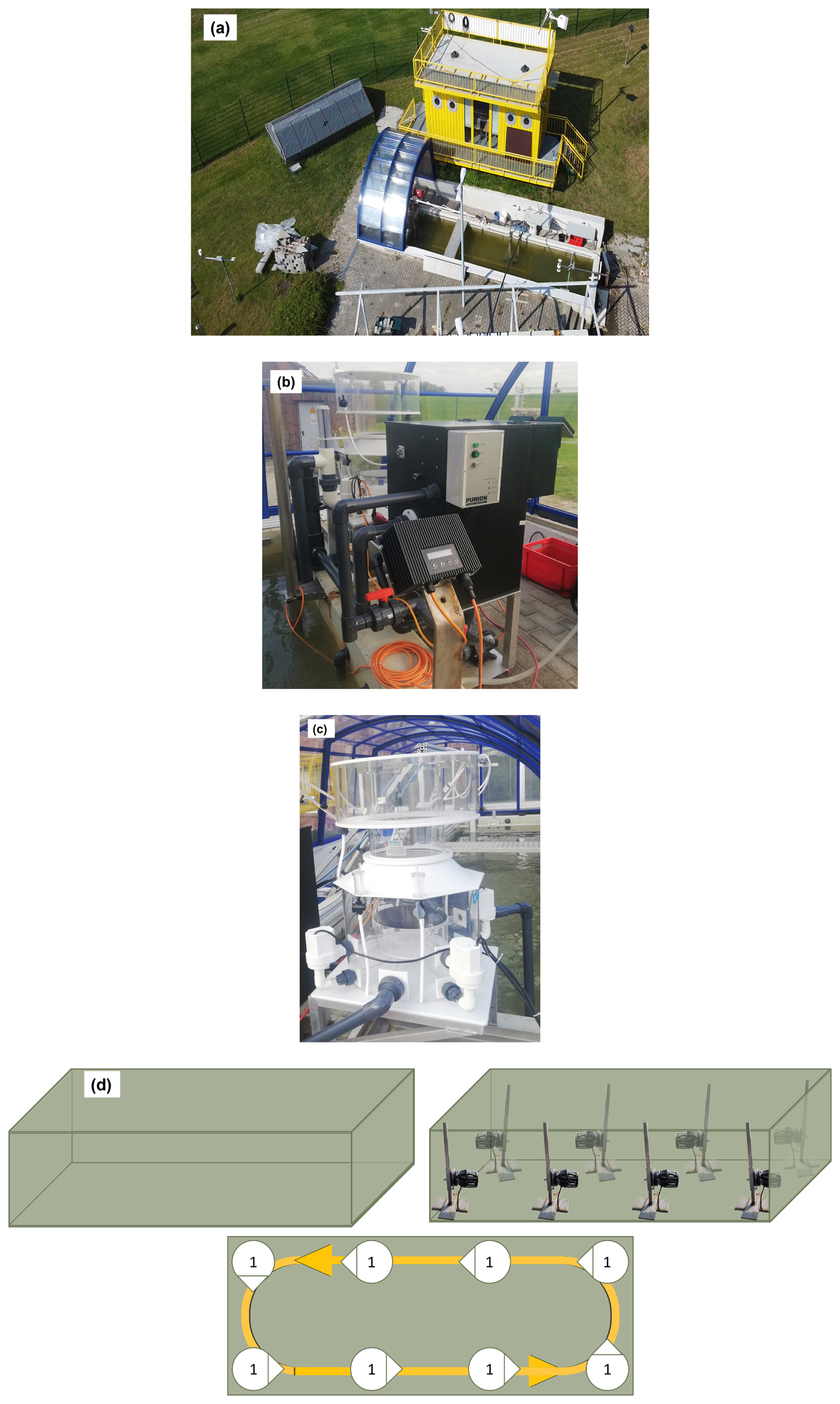
Figure 1 (a) Sea-sURface Facility (SURF) used for the mesocosm experiment. (b) Filtration unit with a fleece filter in the front black box. (c) The Protein skimmer. (d) The top-left panel shows the SURF basin without the pump installed. The top-right panel illustrates the schematic arrangement of eight flow pumps, and the bottom panel shows the direction of the water flow pattern induced by the pumps, ensuring uniform mixing across the basin.

SURF includes a seawater pump that fills the basin with natural seawater from the adjacent Jade Bay (53.467° N, 8.233° E). It further includes several units for seawater pretreatment, such as a large fleece drum filter (Model 300, Ratz Aqua and Polymer Technik, Germany) for removing larger particles and organisms, a protein skimmer (TC12000ix, Deltec GmbH, Germany; Fig. 1b) to eliminate organic material and oxygenate the water (Fig. 1c), and a flow-through UV lamp (Model 2001, Purion GmbH, Germany) to reduce microbial activity. In addition, the basin is equipped with a flow pump (AFC400, Abyzz, Germany) to facilitate water mixing and circulation, a rain simulator (Gassen et al., 2024), and movable platforms for deploying sensors at various depths to record data. The water temperature can be controlled using a heating-cooling system (Titan 6000 Pro, AB Aqua Medic GmbH, Germany), typically within 5 °C of the ambient temperature with an accuracy of ±1 °C. SURF includes a wind machine (TTW 20000, Trotec, Germany) to generate wind speeds of up to 6 m s⁻¹ along the basin. The airflow is centred by a conical outlet attached to the wind machine. Thus, SURF provides a versatile platform for conducting scientific experiments on ocean surface biogeochemistry under diverse and controllable physical conditions.

2.2 Experimental setup

The mesocosm experiment was carried out for 35 d between 15 May (day 1) and 16 June (day 35) 2023. This period in late spring was chosen to have a low initial abundance of phytoplankton in the natural seawater from the adjacent Jade Bay. Complete mixing was achieved by setting the flow pump at 220 m³ h⁻¹. The seawater was filtered through the fleece drum filter (polyester premium filter with 40 g m⁻²) after being pretreated with the protein skimmer and UV lamp. The pre-treatment process resulted in natural seawater with particle concentrations and lower biological activities, as expected for the open sea (e.g. turbidity below 20 Nephelometric Turbidity Units (NTU)).

The experiment was carried out without vigorous mixing in the bulk water, allowing for a water mass with a gentle surface current. This was an important prerequisite for observing processes at a mechanistic level, even though these conditions are rather untypical for the open sea. As the existing flow pump caused excessive turbulent mixing even at the lowest setting, eight smaller pumps (ATK-4 Wavemaker, Aqualight GmbH, Germany, 24 V – 18 m³ h⁻¹, Fig. S1 in the Supplement) were used to ensure the homogeneity of the water column and to reduce particle settling and biofilm formation on walls and bottom of SURF, and stratification during the experiment. The pumps were systematically placed at the bottom of the basin (Fig. 1d). The setup and flow pattern were tested during a pilot phase of the experiment (26 April to 5 May 2023). Each pump had the same power setting and flow angles to simulate slow, natural mixing in the bulk water and its surface without inducing turbulent mixing. To assess homogeneity, turbidity and Chlorophyll a (Chl a) were continuously monitored as baseline parameters using a FerryBox (PocketBox, 4H-Jena, Germany) (Fig. S2; Table S1). The data was used to determine which flow rate and arrangement were most effective in achieving a homogeneous bulk volume in the basin. After the pilot phase, all the instruments and SURF were thoroughly cleaned and prepared for the main phase of the mesocosm experiment.

Five days before the main experiment (11 May), natural seawater from Jade Bay was pumped into a 30 m³ tank. The tank was filled during high tide to minimise the particle load, and an additional two days were allowed for the suspended load to settle. After two days (13 May), the water was pumped from the storage tank into the basin of the SURF. Water was mixed vigorously using the large flow pump for 10 min. Subsequently, fleece filtration and protein skimming were initiated under slow water circulation using eight small flow pumps for three consecutive days. On 15 May, the surface layer of the water column was skimmed with glass plates (Harvey and Burzell, 1972) for nine hours to remove any visible organic film residues and debris from the water surface. SML and ULW water samples were collected on 15 May as time zero (T0). Initial measurements revealed high Chl a fluorescence, which may have been caused by the preparation process, such as filling the SURF with untreated seawater, mixing, and surface skimming. To address this, the water in the SURF was allowed to settle for two days (16–17 May). The time series measurements began on 18 May, as T1, as described in Sect. 2.3. Slow mixing with the smaller flow pumps continued for the whole mesocosm experiment. Natural seawater from Jade Bay was replenished after each sampling to maintain a constant volume in the basin, with 4.5 L per day to replace the volume removed for the SML and UW sampling. The time series included several in situ measurements to monitor the biological, chemical, physical, and optical features of the water at various depths (Table 1).

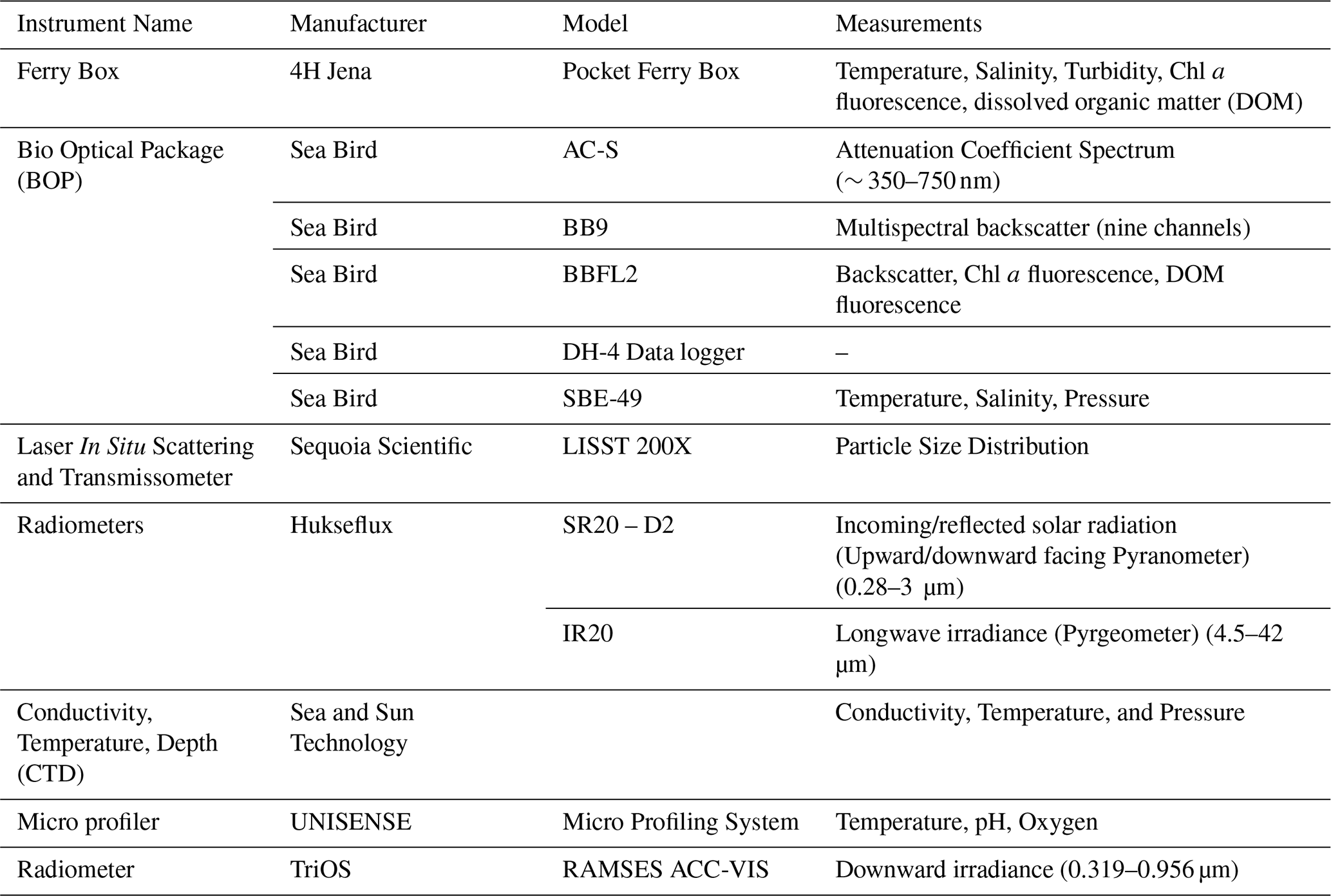
Table 1 Scientific instruments deployed in SURF during the mesocosm for continuous measurements.

2.3 Sample collection

Sampling was conducted on consecutive days, alternating between morning (1 h after sunrise) on the first day and afternoon (10 h after sunrise) on the following day. This sampling strategy was chosen to collect samples exposed to sunlight and darkness. This paper presents only the general time series data, while detailed day and night sampling data and descriptions are provided in other research articles within this special issue. We refrained from more frequent sampling to ensure the continuous integrity of the SML. For the same reason, the volume of the SML collected was limited to 550 mL d⁻¹. This corresponds to approximately 32 % of the total volume of the SML in the basin, assuming the sampled SML is 1000 µm thick.

SML samples were collected using the glass plate technique (Harvey and Burzell, 1972). The glass plate (30 × 25 cm) was immersed vertically into the basin, moving away from the perturbed area and gently withdrawn at a speed of 5–6 cm s⁻¹ (Carlson, 1982). For each sampling, the glass plate was immersed at different spatial locations along the basin for a representative sampling. Adhered SML was collected in acid-washed high-density polyethylene (HDPE) bottles by wiping the glass plate with a squeegee. The water collected from individual dips was pooled to represent an integrated sample. The complete sampling took 20–30 min to collect the target daily SML volume.

ULW samples were collected from a depth of 40 cm using a 60 mL syringe attached to polypropylene tubing. Similar to the SML sampling procedure, the syringe was filled at different locations and then pooled to obtain representative ULW samples of approximately 4 L. Subsamples were taken from the pooled SML and ULW samples for both in situ and laboratory analyses. Sample bottles were gently mixed before subsampling to ensure homogeneous sample distribution. The daily collected SML sample volume was insufficient for analyses of all targeted biogeochemical parameters, so volume-demanding parameters, that is, particulate organic carbon (POC), particulate nitrogen (PN), and photosynthetic pigments, were only determined for the ULW. All the sampling equipment was prewashed with 10 % hydrochloric acid (HCl) and rinsed with ultra-pure water before use to prevent contamination. Samples were collected and handled using polyethylene gloves.

2.4 Inorganic nutrients addition

Inorganic nutrient addition was performed to stimulate a phytoplankton bloom during the mesocosm experiment. Nitrogen, phosphorus, and silicate were added on 26 and 30 May and 1 June 2023. The added nutrient concentrations corresponded to final concentrations of 0, 10, and 5 µmol L⁻¹ for nitrogen and 1.2, 0.6, and 0.3 µmol L⁻¹ for phosphorus, respectively. The additions corresponded to N:P ratios of 0, 16.7, and 16.7, respectively. For silicate, the added concentrations corresponded to final concentrations of 19.8, 10, and 0 µmol L⁻¹, respectively. Nutrients were added by drawing a tube from the bottom to the top of the water column at different locations in the basin to ensure even distribution.

2.5 Analysis of inorganic nutrients and surfactants

Subsamples from the SML and ULW (40 cm depth) were collected in HDPE bottles and filtered with surfactant-free cellulose acetate (SFCA) membrane filter (0.45 µm) to measure nitrite (NO${}_{\mathrm{2}}^{-}$), nitrate (NO${}_{\mathrm{3}}^{-}$), phosphate (PO${}_{\mathrm{4}}^{\mathrm{3}-}$), and silicate (Si(OH)₄) concentrations. All samples were poisoned with mercury chloride and stored at 4 °C for further analysis in the laboratory (Kattner, 1999). Nutrient concentrations were determined using a sequential automatic analyser (SAA, SYSTEA EASYCHEM) and with the microtiter plate technique according to methods described by Fanning and Pilson (1973); Miranda et al. (2001); Doane and Horwáth (2003); Laskov et al. (2007) and Schnetger and Lehners (2014). The detection limits were 0.4 µM for nitrate and nitrite, 0.04 µM for phosphate, and 0.1 µM for silicate. The analytical error for nutrient quantifications was less than 10 %.

Subsamples from the SML and ULW for surfactant analysis were collected in 50 mL non-transparent HDPE bottles and stored at 4 °C. To retain the particulate fraction of surface activity (Ćosović, 1987; Wurl et al., 2011), unfiltered samples (10 mL) were analysed in triplicate using a standard addition technique (Ćosović, 1987). The concentrations of surfactants were measured by a voltammetry technique (797 VA Computrace, including 863 Compact Autosampler, Metrohm, Switzerland) with a hanging drop mercury electrode (Ćosović, 1987). Calibration via standard addition was performed by adding a Triton X-100 stock solution. The concentrations of surfactants are expressed as µg Triton X-100 equivalent L⁻¹ (µg Teq L⁻¹). A sodium chloride solution (NaCl) with a concentration of 32 g L⁻¹ was used as a blank. The analytical error of the measurements for surfactants was less than 10 %.

In addition to voltammetry, surface-sensitive non-linear vibrational sum-frequency generation (VSFG) spectroscopy was employed to characterise the presence of a molecular film of surfactants directly at the air-water interface on a nanometer scale. SML samples were collected in 50 mL PP bottles and subsequently frozen at −20 °C for further analysis in the laser laboratory. Details of the analysis procedure can be found in the Supplement (including Fig. S3), and the use of VSFG for SML surfactant film analysis has been outlined elsewhere (Laß and Friedrichs, 2011; Laß et al., 2013; Engel et al., 2018). For each sampling day, an average of 3–5 spectra was recorded using 10 mL aliquots of the daily sample. Surfactant film abundance is reported in terms of an operationally defined surface coverage index sc.It is calculated from the ratio of integrated spectral intensities over the CH-stretch vibrational range, referenced to the spectrum of a well-defined dense surfactant monolayer of dipalmitoylphosphatidylcholine (DPPC) with a surface concentration of 0.22 nmol cm⁻². In simplified terms, surface coverage index values of sc = 0 % or sc = 100 % can be interpreted as a surfactant-free or a fully covered molecular film of surfactant-like material directly at the air-water interface, respectively. Within the scope of validity of the model approach, the analytical precision can be estimated as Δsc = 10 % (2σ), based on error propagation of the relative 1σ repeatability of the individual spectra of 6 %.

2.6 Analysis of carbon and nitrogen (total, dissolved, and particulate)

For dissolved organic carbon (DOC), two sets of samples were prepared and analysed at ICBM (Oldenburg) and GEOMAR (Kiel), and the results were integrated. Details of the DOC interlaboratory comparison are provided in the Supplement (including Figs. S4–S6). Total dissolved nitrogen (TDN) was quantified at GEOMAR. SML and ULW samples were primarily filtered through glass microfibre ?lters (Whatman). The first sample set was stored in acid-rinsed HDPE bottles at −18 °C. The second set was acidified, sealed in pre-combusted glass ampules, and stored at +4 °C until analysis. All samples were acidified to pH 2 prior to the measurement of DOC and TDN. DOC concentrations were measured using a Shimadzu TOC Analyser (TOC-L or TOC-VCPH) following the high-temperature catalytic oxidation method (Sugimura and Suzuki, 1988). Acidification of samples oxidises inorganic carbon to CO₂, which was purged with synthetic air to remove the CO2. Subsequently, the remaining organic carbon was converted to CO₂ through a platinum-catalyzed oxidation at 720 °C. The resulting CO₂ was measured using a non-dispersive IR gas analyser. Each sample was injected four times and the values were averaged. Calibration was performed using a potassium hydrogen phthalate and a potassium nitrate standard, for DOC and TDN, respectively. Accuracy was verified using certified deep-sea reference material (David A. Hansell, University of Miami, FL, USA).

ULW sample aliquots for POC and PN analysis were filtered at a low, constant vacuum (< 0.2 bar) onto GF/F filters (Whatman, 25 mm, pre-combusted for 8 h at 500 °C) in triplicate, with volumes ranging from 20 to 270 mL per filter. After filtration, the filters were stored in 2 mL Eppendorf tubes at −20 °C until further analysis. Duplicate filters were exposed to 37 % fuming HCl in a fuming box for at least six hours to remove inorganic carbon. Acidified filters were dried at 60 °C for 12 h. Both acidified and non-acidified filters were wrapped in tin cups and measured using a Euro EA elemental analyser (EVR 3000, HEKAtech, Germany) calibrated with an acetanilide standard according to Sharp (1974).

2.7 Photosynthetic pigments and phytoplankton community composition

Phytoplankton pigment concentrations were analysed using high-performance liquid chromatography (HPLC) according to Zapata et al. (2000). Subsamples of approximately 1 L volume from the ULW were filtered through pre-combusted GFF filters (Whatman, 47 mm). The filters were immediately shock-frozen in liquid nitrogen and stored at −80 °C until HPLC analysis. Shortly before analysis, the pigments were extracted in 2–4 mL of 100 % acetone for 24 h in the dark at −20 °C using 20 mL glass scintillation vials. The extracts were cleared of particles by filtration using 5 mL syringes and 0.2 µm syringe filters (Spartan 13A). They were then filled into 2 mL autosampler vials and analysed using a Shimadzu HPLC system. Several diagnostic pigments were selected as biomarkers for different phytoplankton taxa observed during the experiment. These included Chlorophyll b (Chl b), Chlorophyll c (Chl c), fucoxanthin, 4-keto-19^′-hexanoyloxyfucoxanthin, cis-fucoxanthin, diadinoxanthin, diatoxanthin, β-carotene, and echinenone.

An imaging particle analyser (FlowCam 8400, Yokogawa Fluid Imaging Technologies, USA) was used to analyse the SML and the ULW samples for particle number and type, including the identification and quantification of phytoplankton cells. Particles of 1 mL of the sample were imaged at 100× magnification using a flow cell with an orifice of 100 µm. The samples were prefiltered through a 100 µm nylon mesh to prevent clogging of the flow cells. As mainly larger cells were expected to dominate the bloom, an automated digital size filter was applied during image acquisition to exclude particles < 10 µm, to prevent the sample files from becoming too large, and to facilitate efficient data analysis. Sample analysis was performed without replicates; however, to estimate the accuracy of the obtained particle counts, three replicates from selected samples were conducted three times during the experiment. From this, a counting error of approximately 16 % was calculated (data not shown). This is consistent with previous, similar experiments. After a manual quality check of the images, they were classified using the built-in software Visual Spreadsheet 5. The libraries used for classification contained 40–60 images selected from different samples of the experiment, and, if necessary, multiple libraries were used for a given type of particle.

A LISST-200X (Sequoia Scientific, USA) was mounted on a frame submerged in the SURF basin. The instrument estimates particle size distribution based on forward light scattering. Measurements were conducted 4 to 10 times per day, averaging 10 min, to ensure that the sampling time was also covered.

2.8 Bacterial cell counts and metabolic profiles

The bacterial abundance in the SML and the ULW was evaluated using flow-cytometric cell counts. Subsamples for flow-cytometric enumeration of cells were pre-filtered through 5 µm polycarbonate membrane filters (Whatman, Cytiva Life Sciences, USA, 47 mm diameter) to remove debris and transferred into clean 250 mL polycarbonate bottles. 1730 µL of the prefiltered subsamples were fixed by adding 70 µL of electron microscopy grade glutaraldehyde (GDA, 1 % final concentration, Sigma-Aldrich, Germany) and incubated at 4 °C for 30 min. The fixed samples were then frozen at −80 °C until further analysis. Frozen samples were thawed in ice-cold water and diluted 1:10 with sterile, filtered TE buffer (10 mM Tris, 1 mM EDTA, pH 8). The samples were stained with SYBR^™ Green I nucleic acid stain (Invitrogen, Thermo Fischer Scientific) at a final concentration of 1:10 000 and incubated in the dark at room temperature for 10 minutes. Total bacterial cells were counted with a BD FACSAria III flow cytometer (BD Biosciences, USA), equipped with a 488 nm blue laser and a 530/30 band-pass filter for SYBR^™ Green fluorescence detection. Before each analytical run, the instrument was calibrated using the Cytometer Setup and Tracking (CST) routine with fluorescent bead standards (Fluoresbrite^® YG Microspheres, Polysciences, Inc., USA) to verify optical alignment and detector sensitivity.

Forward- and side-scatter properties were used to differentiate bacterial populations. Instrument settings were optimised as described in Brussaard et al. (2010), including appropriate voltages for scatter (470 and 500 V for forward and side scatter, respectively) and fluorescence detection (500 V) to maximise the resolution of bacterial populations. To ensure accurate quantification, the flow rate was calibrated using gravimetric measurements of Milli-Q water (triplicate weight–time determinations). Data were analysed using BDFACSDiva v.6.1.3 software (BD Biosciences, USA), and bacterial cell counts were normalised to cells × 10⁹ L⁻¹, accounting for the flow speed during measurement and the dilution factor.

The bacterial gate was first defined in the SYBR^™ Green fluorescence versus SSC-H plot, capturing the central cluster of events with intermediate fluorescence and side scatter. The lower boundary was adjusted to exclude weakly fluorescent debris, while the upper boundary excluded larger, more fluorescent particles such as picoeukaryotes or organic flocs. Gate placement was validated by cross-checking the same population in FSC-H vs SSC-H and SYBR Green vs FSC-H plots, ensuring that only the prokaryotic-sized fraction was included (Figs. S7–S8 for representative gating and blank controls). The same gate boundaries were applied to all samples to maintain comparability. A fluorescence threshold of 200 arbitrary units was applied to the SYBR Green channel to suppress noise and exclude non-fluorescent particles. Blank and bead controls confirmed that no significant signal overlapped with the prokaryotic gate.

Biolog EcoPlate^™ (Cat #1506; Biolog, Hayward, CA, United States) was used to evaluate the metabolic profiles of the microbial communities by assessing the carbon utilisation in the SML and the ULW samples. The EcoPlate^™ consists of 31 substrates, including polymers, amino acids, amines, carboxylic acids, carbohydrates, and one blank. Unfiltered SML and ULW subsamples were added to the wells (150 µL per well) and incubated at room temperature in the dark for 1 week. Each sample was analysed in triplicate. Substrate utilisation was indicated by a colour change due to the reduction of a tetrazolium dye that produces a measurable colour signal as bacteria respire and quantified by measuring the optical density at a wavelength of 590 nm using a microplate-reader spectrophotometer (Multiskan GO, Thermo Fisher Scientific, Finland), equipped with an automatic plate reader. Measurements were taken every 24 h over a 7 d incubation period. The average well colour development (AWCD) was calculated as a proxy for the overall metabolic activity of the bacterial community. The average substrate colour development (ASCD), was used to assess substrate-specific utilisation (Garland, 1996). Additionally, the N-index, which represents the percentage of the utilised substrate containing nitrogen, was systematically determined by summing the AWCD of all nitrogen-containing substrates at a wavelength of 590 nm. No control incubations were performed.

2.9 Statistical analysis

All biogeochemical variables were tested for normality using the Shapiro–Wilk test. A p-value greater than 0.05 was considered indicative of a normal distribution. However, the p-values for all biogeochemical variables were less than 0.05, indicating that the data deviates from a normal distribution. So, a non-parametric Kruskal–Wallis test was performed to check the difference between SML and ULW for the parameters, which have data from both layers, including NO${}_{\mathrm{2}}^{-}$, NO${}_{\mathrm{3}}^{-}$, Si(OH)₄, PO${}_{\mathrm{4}}^{\mathrm{3}-}$, N:P ratio, surfactants, DOC, and TDN. Spearman's rank correlation was used to determine the relationship between biogeochemical variables. Enrichment factors (EFs) were calculated as EF = $C_{\mathrm{SML}}/C_{\mathrm{ULW}}$, where C_SML and C_ULW are the concentrations of the variable in the SML and ULW, respectively. Enrichment of a variable in the SML was indicated when the EF was greater than 1, while depletion was indicated when the EF was less than 1.

A self-organising map (SOM) was used to characterise the distribution patterns and temporal variability in nutrient data. SOM is an unsupervised artificial neural network that projects high-dimensional multivariate data (nutrients in the SML and the ULW in this study) onto a two-dimensional gridded space to cluster and visualise the properties of the input data (Kohonen, 2001; Kohonen, 2013). The SOM algorithm network consists of the input and output layers. In the training process, the SOM algorithm utilises an input layer (nutrient data in this study) comprising 60 nodes, one for each sampling date, connected to the sampling datasets of the two water layers, i.e., the SML and ULW. During the subsequent learning and training phases, the data are assigned to output neurons in the output layer. The training process determines the “best-matching unit” based on the Euclidean distance measure, and samples of similar characteristics are classified either in the same neuron or adjacent neurons according to the degree of similarity.

The output layer, comprising 36 neurons, was organised and visualised in a 6 × 6 hexagonal grid. The SOM grid or number of output neurons was chosen based on $M\approx \mathrm{5}\sqrt{N}$, where N is the number of samples according to Vesanto and Alhoniemi (2000). The final size of the SOM was decided based on the minimum best values of the quantisation error (QE) and topographic error (TE) by running the entire procedure several times (Park et al., 2003). QE and TE are key metrics for assessing the quality of the SOM. QE quantifies the proximity of input data points to their best-matching unit (BMU) on the SOM, evaluating how well the map represents the input data. Essentially, QE reflects variance and is an accuracy measure (Kohonen, 2001). TE assesses topology preservation and indicates how well the trained SOM model preserves the relationships or structure of the input dataset. Lower QE and TE values signify higher-quality SOM (Bauer et al., 1999).

A SOM map with QE and TE values of 0.11 and 0.00, respectively, was selected. Ward's linkage method, using the Euclidean distance measure, was then applied to define the cluster boundaries between different SOM units and subdivide them into groups based on similarity among the neurons (Legendre and Legendre, 2012). The R package kohonen was used to train the SOM model. Hierarchical cluster analysis, using the cutree and hclust functions of dendextend package (Galili, 2015), was performed to define clusters (based on SOM output) that were characterised by different colors. NbClust package was used to determine the optimal number of clusters (Charrad et al., 2014). Before SOM training, two extreme values in PO${}_{\mathrm{4}}^{\mathrm{3}-}$ and one in Si(OH)₄ were removed, and nutrient data were normalised on a scale of 0–1 to ensure that all the nutrients have equal importance in generating the SOM map. All the statistical analyses, including the SOM and the clustering, were performed using R software, version 4.1.2 (R Core Team, 2020).

3 Results

The observed shift in phytoplankton biomass (using Chl a concentration as a proxy) and community composition in response to nutrient variability followed a characteristic bloom succession during the mesocosm experiment. The synergistic relationship between Chl a, particulate organic carbon (POC), and particulate nitrogen (PN) suggests that phytoplankton dynamics played a vital role in organic matter (OM) production and distribution during the study period. A mismatch between Chl a and surfactant concentrations suggests that phytoplankton's physiological response to nutrient stress, particularly during the post-bloom phase, was a strong predictor of surfactant accumulation in the sea surface microlayer (SML), driven by phytoplankton exudates and the microbial degradation of organic matter. The presence of a distinct SML, enriched in surfactants and OM (slick formation), acted as a microbial habitat, leading to increased bacterial abundance in the SML.

3.1 Hydrographic conditions

The diurnal temperature, salinity, and turbidity data are presented in Fig. S9a–c. The daily average temperature ranged from a minimum of 16.8 °C in May to a maximum of 23.6 °C in June, with an average temperature of 19.8 °C. The diurnal fluctuation in temperature was typically 8.7 °C. Overall, the temperature increased from the first week of June onwards and remained consistently high in the last few days of the experiment (Fig. 2a). Temperature profiles across the upper 5 mm, including the SML, were recorded using microsensors and are reported in Rauch et al. (2025). We have included only the ULW data in Fig. 2. Salinity showed an increasing trend as well, from 29.2 to 32.3 g kg⁻¹ (Fig. 2a). Higher temperatures enhanced evaporation, resulting in a higher concentration of salt in the SURF basin. In comparison to the temperature, salinity increased steadily until the end of the experiment. Salinity in the SML could not be quantified accurately in discrete water samples (with a precision of > 0.005 g kg⁻¹) due to evaporative water losses during handling.

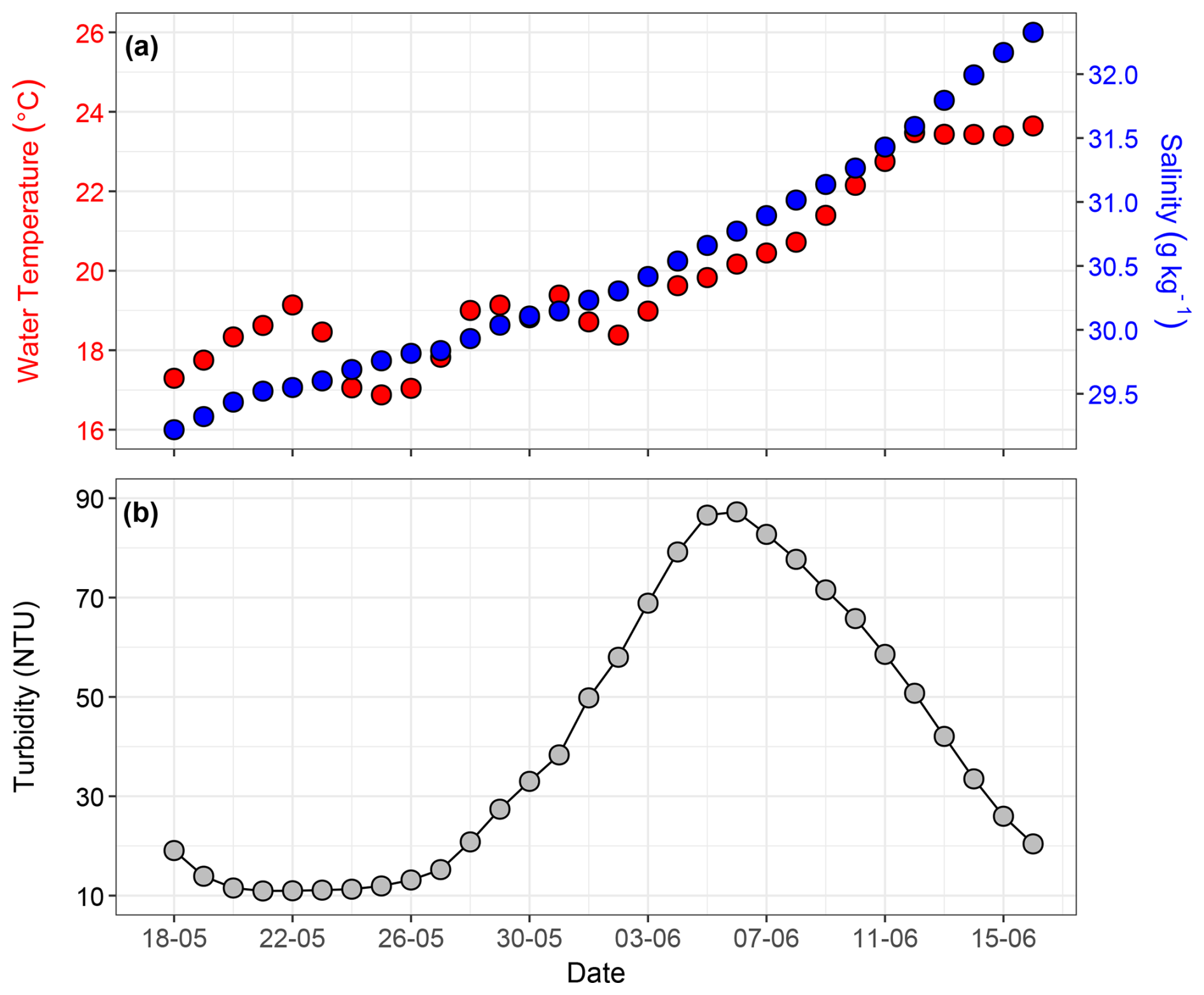
Figure 2 Time series of daily average values for (a) water temperature (°C) and salinity (g kg⁻¹), and (b) turbidity (NTU). The hydrographic parameters were monitored only in the ULW.

The daily average turbidity in the SURF basin varied from 10.9 to 87.2 NTU. It remained relatively low and stable from 18 to 26 June, consistent with early spring conditions and lower biological activity during the pre-bloom phase of the mesocosm. Turbidity steadily increased from 27 May onward, peaking between 4–6 June (Fig. 2b), primarily due to the release of coccoliths into the water column. This caused the water to appear milky and more turbid. The turbidity peak occurred after the Emiliania huxleyi bloom and shortly after the diatom bloom, as also evident in the LISST and HPLC data described later in the results.

3.2 Solar irradiance and meteorological data

Continuous time series measurements of incoming and reflected solar irradiance (W m⁻²) and albedo (%) over the study period are shown in Fig. S10a–c. To derive daytime albedo values and obtain comparable light intensity measurements under consistent daylight conditions, daily averages were calculated during the period of maximum sunshine hours (09:00 to 16:00 local time). The daily average incoming solar irradiance varied from 74 W m⁻² on May 22 to 753 W m⁻² on 7 June, with an average of 576 W m⁻² throughout the experiment. Incoming solar irradiance fluctuated (Fig. 3a) and was low on specific days in late May (22, 24, and 31 May) and early June (1 June) due to precipitation and cloud cover. These low values coincided with lower air temperatures. Daily average reflected solar irradiance varied from 3 to 70 W m⁻². During the pre-bloom and bloom phase, reflected solar irradiance varied between 3 and 51 W m⁻² . During the post-bloom phase, a steady increase in reflected solar irradiance was observed, peaking at 70 W m⁻² (Fig. 3b). Daily average albedo varied from 3.8 % to 9.4 % and remained relatively stable (∼ 4 %–5 %) until 30 May, followed by a sharp increase from 31 May to 6 June (Fig. 3c). This peak coincided with a high assemblage of coccoliths (particles of 3–4 µm), indicating that the calcium carbonate plates shed by Emiliania huxleyi during the bloom phase contributed to enhanced reflection and increased albedo.

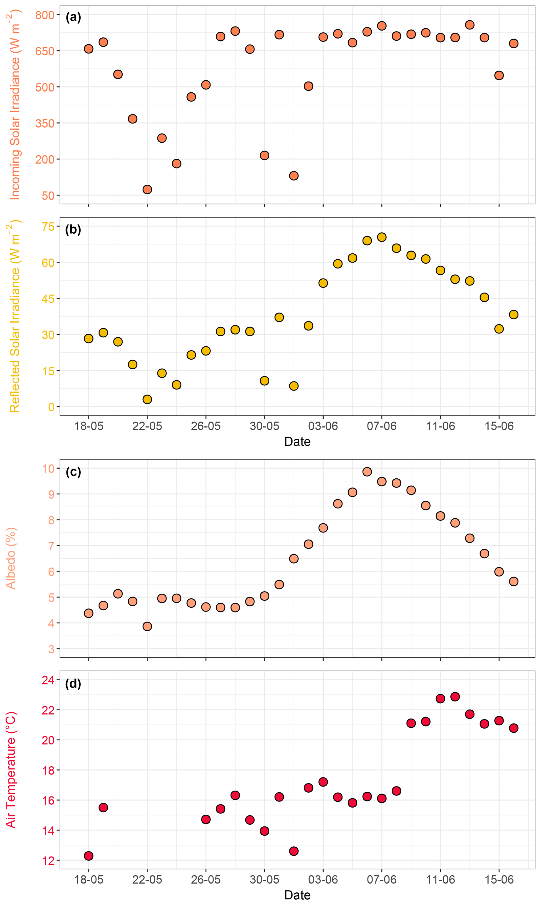
Figure 3 Time series showing averages over the period of maximum sunshine hours (09:00–16:00 local time) for (a) incoming solar irradiance (W m⁻²), (b) reflected solar irradiance (W m⁻²), and (c) albedo (%). Panel (d) shows daily average air temperature (°C), with gaps indicating days when air temperature records from the weather station were unavailable.

Air temperature exhibited clear seasonal trends from May to June and short-term temporal fluctuations, with the highest daily average reaching 22.8 °C on 12 June, reflecting sunny summer conditions in the region (Figs. 3d, S10d). The lowest daily average, 12.2 °C, was recorded on 18 May, highlighting cooler late-spring conditions. Throughout June, air temperature showed sharp fluctuations, indicating transient weather patterns, such as changes in cloud cover and precipitation.

3.3 Inorganic nutrient concentrations

All nutrients exhibited temporal variations throughout the mesocosm experiment. Nutrient concentrations in the SML were generally more variable than those in the ULW (Fig. 4a–d). NO${}_{\mathrm{3}}^{-}$ was the dominant nitrogen species, with concentrations ranging from < 0.1 to 12.1 µmol L⁻¹ in the SML and < 0.1 to 12.2 µmol L⁻¹ in the ULW during the pre-bloom phase. A distinct drawdown of NO${}_{\mathrm{3}}^{-}$ was observed as the bloom phase progressed. This sharp decline corresponded with an increase in phytoplankton biomass, as indicated by a rise in Chl a. The SML and the ULW samples showed statistically significant differences (p<0.05) in NO${}_{\mathrm{3}}^{-}$ concentrations. The addition of inorganic nitrogen on 30 May (10 µmol L⁻¹) and 1 June (5 µmol L⁻¹) led to an increase in NO${}_{\mathrm{3}}^{-}$ concentration by 2 June. However, it remained low in both water layers throughout the mesocosm experiment, indicating continuous biological uptake, particularly during the bloom phase (Fig. 4a).

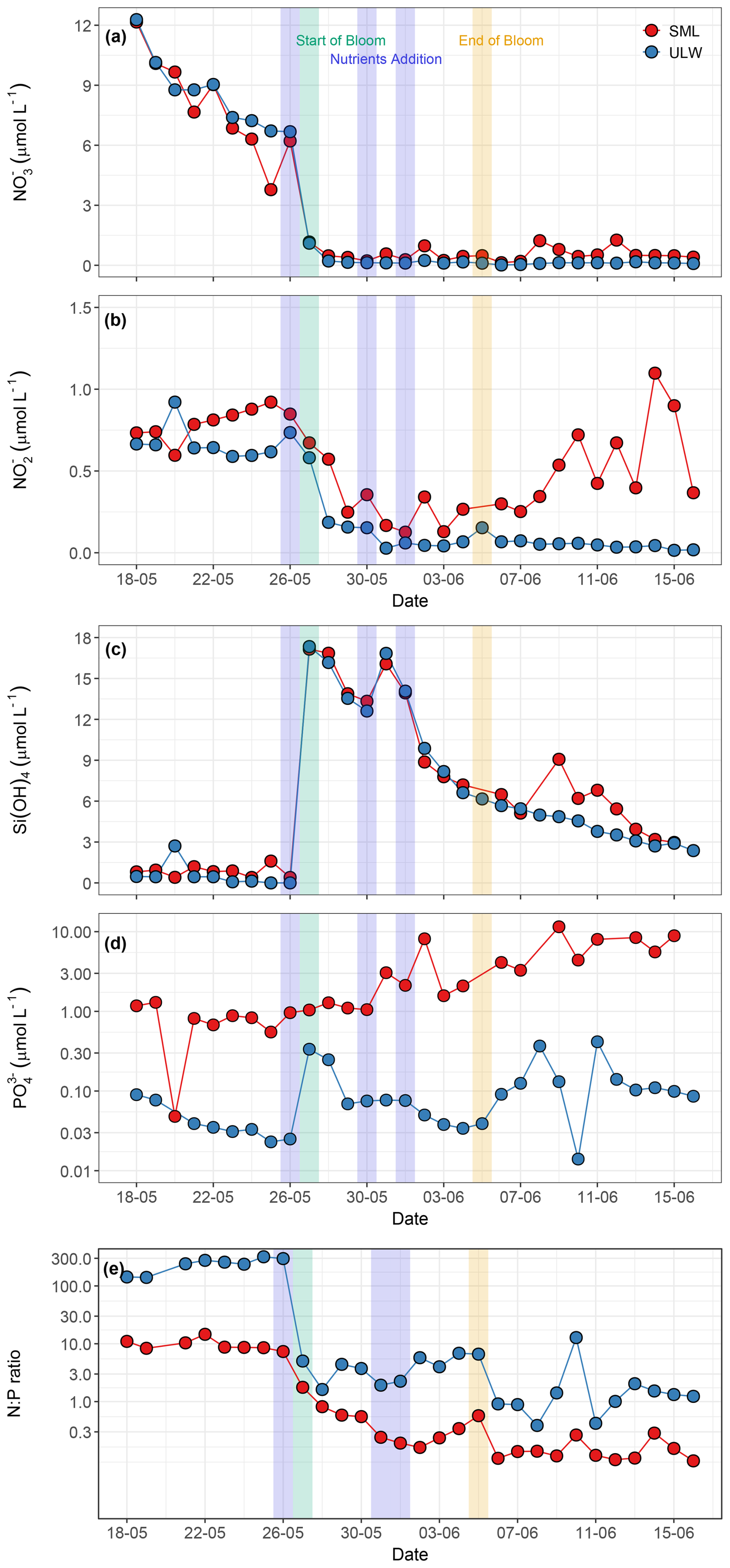
Figure 4 Temporal distribution patterns of (a) nitrate (NO${}_{\mathrm{3}}^{-}$, µmol L⁻¹), (b) nitrite (NO${}_{\mathrm{2}}^{-}$, µmol L⁻¹), (c) silicate (Si(OH)₄, µmol L⁻¹), (d) phosphate (PO${}_{\mathrm{4}}^{\mathrm{3}-}$, µmol L⁻¹), and (e) N:P ratios in the SML and the ULW. Panels (d) and (e) use a logarithmic y axis. In all the panels, red circles represent SML, whereas blue circles represent ULW. The blue shaded parts in all the panels mark the dates of nutrient addition (26 and 30 May, and 1 June), the green shaded part marks the start date of the bloom phase (27 May), and the yellow shaded part marks the termination date of the bloom phase (5 June).

NO${}_{\mathrm{2}}^{-}$ concentrations ranged from 0.1 to 1.1 µmol L⁻¹ in the SML and < 0.1 to 0.9 µmol L⁻¹ in the ULW (Fig. 4b), exhibiting a statistically significant difference between the SML and the ULW samples (Kruskal–Wallis test, p<0.05). The NO${}_{\mathrm{2}}^{-}$ concentration remained relatively constant during the pre-bloom phase and decreased significantly in the SML and the ULW during the bloom phase before inorganic nitrogen was added on 30 May. A sharp increase in the NO${}_{\mathrm{2}}^{-}$ concentration was observed in the SML during the bloom phase, which progressed into the post-bloom phase. However, the NO${}_{\mathrm{2}}^{-}$ concentration remained low in the ULW during the bloom and post-bloom phases.

Si(OH)₄ concentrations ranged from 0.4 to 1.6 µmol L⁻¹ in the SML and from < 0.1 to 2.7 µmol L⁻¹ in the ULW during the pre-bloom phase and remained relatively stable in both layers until the first addition of nutrients (19.8 µmol L⁻¹ of Si(OH)₄) on 26 May. After nutrient addition, a sharp increase in Si(OH)₄ concentrations was observed in both the SML (17.1 µmol L⁻¹) and the ULW (17.3 µmol L⁻¹) on 27 May (Fig. 4c). A decrease in phytoplankton biomass (Chl a concentration) as well as in Si(OH)₄ concentration (∼ 4 µmol L⁻¹) was observed on 29 May. For this reason, a second addition of 10 µmol L⁻¹ Si(OH)₄ was carried out the following day, leading to an increase in Si(OH)₄ of 16.1 and 16.8 µmol L⁻¹ in the SML and the ULW, respectively. No statistically significant difference was detected between the SML and the ULW regarding Si(OH)₄ concentrations (Kruskal–Wallis test, p= 0.19).

The concentrations of PO${}_{\mathrm{4}}^{\mathrm{3}-}$ ranged from < 0.1 to 11.52 µmol L⁻¹ in the SML. In the ULW, concentrations remained near the detection limit before the addition of inorganic phosphorus. Even after the addition, PO${}_{\mathrm{4}}^{\mathrm{3}-}$ concentrations in the ULW remained low throughout the mesocosm experiment (Fig. 4d). Concentrations of PO${}_{\mathrm{4}}^{\mathrm{3}-}$ between the SML and the ULW were statistically different (Kruskal–Wallis test, p = 0.04). For example, PO${}_{\mathrm{4}}^{\mathrm{3}-}$ levels in the SML increased almost threefold during the bloom phase after inorganic phosphorus was added on 30 May. This increase indicates microbial release and OM recycling in the SML during the bloom and post-bloom phases.

The N:P ratios ((NO${}_{\mathrm{3}}^{-}+$ NO${}_{\mathrm{2}}^{-}$) : PO${}_{\mathrm{4}}^{\mathrm{3}-}$) varied from 0.0 to 318.8 and were significantly high in the ULW (Kruskal–Wallis test, p<0.05) compared to the SML during the pre-bloom phase and remained consistently elevated in the ULW throughout the mesocosm experiment. Although the N:P ratio was substantially higher in the ULW, it remained at ∼ 10 in the SML during the pre-bloom phase (Fig. 4e). These temporal patterns of nutrient stoichiometry highlight the link between phytoplankton-driven biological activity, nutrient availability, and covariance with other favourable environmental conditions such as light, and temperature during the seasonal transition.

3.4 Phytoplankton biomass (Chl a) and community composition

Phytoplankton biomass and other phytoplankton pigments were measured exclusively in the ULW as proxies to track the growth dynamics and community structure of phytoplankton during the mesocosm experiment. Temporal trends showed that the Chl a concentration varied from 1.0 to 11.4 µg L⁻¹ and exhibited significant variations (Fig. 5a). The mesocosm experiment was hence divided into three distinct phases: pre-bloom, bloom, and post-bloom. The pre-bloom phase (18 to 26 May) occurred before nutrients were added, with an average Chl a concentration of 2.2 µg L⁻¹ . The bloom phase (27 May to 5 June), was marked by a rapid proliferation of phytoplankton biomass, as indicated by elevated Chl a concentrations, with an average of 7.3 µg L⁻¹ . In contrast, the post-bloom phase lasted from 5 June until the end of the mesocosm experiment. A low Chl a concentration, averaging 1.8 µg L⁻¹, was observed during this phase.

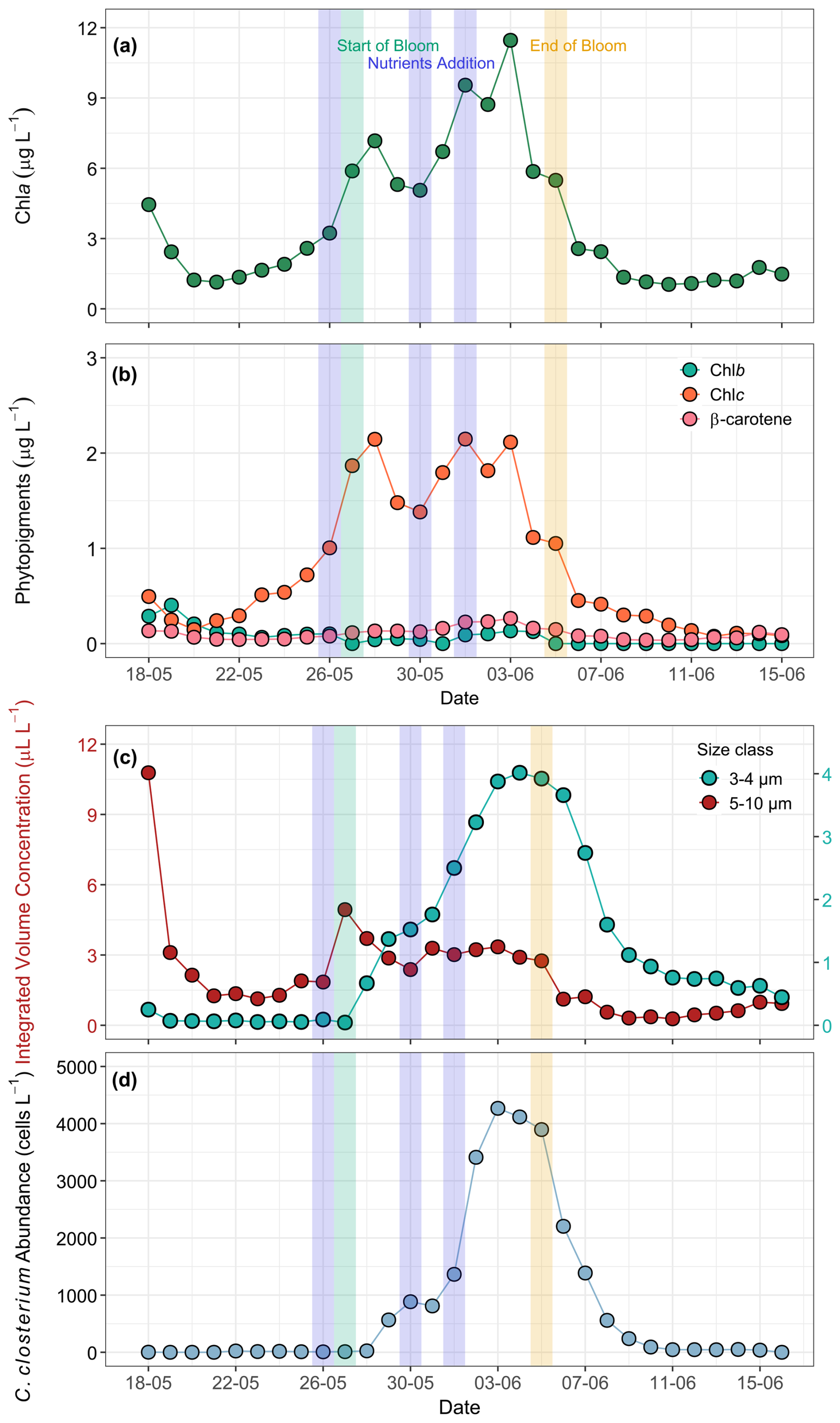
Figure 5 Temporal development of phytoplankton bloom dynamics during the mesocosm experiment. (a) Chl a (µg L⁻¹) as a proxy for phytoplankton biomass, (b) concentrations of Chl b, Chl c, and β-carotene (µg L⁻¹), (c) LISST-derived particle distribution showing integrated volume concentration (µL L⁻¹ ) for size classes: 5–10 µm (coccolithophores, presumably Emiliania huxleyi) and 3–4 µm (detached coccoliths). (d) FlowCam-derived counts of Cylindrotheca closterium abundance (cells L⁻¹). Phytopigments and optical measurements were performed only on ULW samples. The blue shaded parts in all the panels mark the dates of nutrient addition (26 and 30 May May, and 1 June), the green shaded part marks the start date of the bloom phase (27 May), and the yellow shaded part marks the termination date of the bloom phase (5 June).

HPLC-based phytopigments showed the highest concentration of Chl c, a marker pigment for haptophytes. Haptophytes are a phytoplankton group that also includes coccolithophores, such as Emiliania huxleyi. Chl b, a pigment associated with chlorophytes and β-carotene, which is widely linked to chlorophytes, dinoflagellates, and prasinophytes, contributed minimally to the total phytoplankton biomass (Fig. 5b). All pigment concentrations declined after the bloom peak, remaining at lower, constant levels. The temporal trends and synchronicity between Chl a and other phytopigment concentrations highlight a well-defined bloom cycle driven by nutrient gradient and the role of phytoplankton communities in shaping the overall biomass dynamics during the bloom phase.

Additional characterisation of phytoplankton response to nutrient addition and bloom progression was provided by data from the LISST-200X, conventional microscopy, and FlowCam, respectively. The two dominant bloom-forming species were the diatom Cylindrotheca closterium and the haptophyte Emiliania huxleyi. Identification of Cylindrotheca closterium was done by FlowCam imaging, while Emiliania huxleyi was identified by scanning electron microscopy (SEM) via the specific structure of their coccoliths (Fig. S11). Due to the applied image acquisition size filter of 10 µm, Emiliania huxleyi was not detected and counted until the last days of the experiment. In order to still provide an estimation on the development of this species during the experiment, we made two assumptions: (i) particles in the size range of 5–10 µm were mainly Emiliania huxleyi, as this range corresponds the cell size of the species, and significant numbers of small, round cells of this size were detected in the FlowCam data after the digital size filter was removed (data not shown); and (ii) particles in the size range 3–4 µm were primarily detached coccoliths of Emiliania huxleyi. Based on these assumptions, we used the integrated size bins from the LISST-derived particle size distribution that corresponds to the average size of Emiliania huxleyi cells (5–10 µm) as a proxy for the development of its population. Similarly, the size bins covering 3–4 µm were used as indicators for free coccoliths, whose presence was also observed microscopically and which likely contributed strongly to the increased turbidity of the water towards the end of the experiment (Figs. 5c and 2b). However, other contributors to the turbidity cannot be excluded. While the first nutrient addition triggered the bloom of Emiliania huxleyi, a high concentration of Si(OH)₄ from the second nutrient addition favoured the growth of diatoms (Cylindrotheca closterium) as shown by the FlowCam-derived counts (Fig. 5d). Thus, the first bloom peak (28 May) was dominated by Emiliania huxleyi, while the second, larger peak (3 June) coincided with a high abundance of Cylindrotheca closterium.

3.5 Surfactants and organic matter composition

Surfactant concentrations varied over a wide range from 89.6 to 1963.2 µg Teq L⁻¹ in the SML and a narrower range from 46.6 to 313.7 µg Teq L⁻¹ in the ULW. Surfactants were significantly enriched in the SML compared to the ULW (Kruskal–Wallis test, p= 0.01, Fig. 6a), with EFs ranging from 0.5 to 15.3 (3.2 ± 3.1) (Fig. S12). Maximum EFs were observed after the bloom phase (Fig. 6a), as bloom decay increased the fraction of surfactants and degraded OM, leading to their accumulation in the SML. A slight increase in surfactants in the SML was observed after the first addition of nutrients. However, we observed a pronounced time lag between the onset of the increases in phytoplankton biomass and surfactant concentrations (Fig. 5a), with surfactant concentrations peaking five days after the onset of the bloom phase. Although the surfactant concentrations decreased toward the end of the experiment, two peaks were observed on 12 and 14 June, each exceeding 1000 µg Teq L⁻¹, surpassing the general threshold concentration for slick formation (Wurl et al., 2011). Surfactant concentrations in the ULW remained consistently lower (< 313.7 µg Teq L⁻¹) with only minor variations throughout the mesocosm.

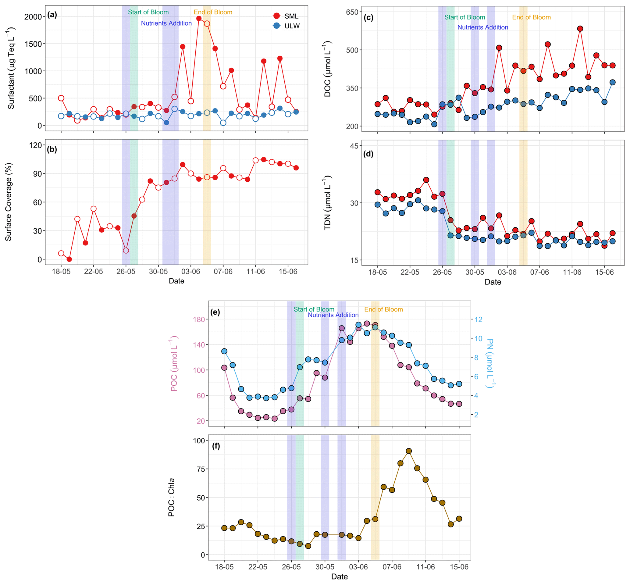
Figure 6 Temporal distribution patterns of (a) surfactant concentrations (µg Teq L⁻¹), (b) surface coverage (with open and filled circles representing morning and evening samples, respectively), (c) dissolved organic carbon (DOC, µmol L⁻¹), and (d) total dissolved nitrogen (TDN, µmol L⁻¹) in SML and ULW. The red circles in panels (a), (c), and (d) represent SML, and the blue circles represent ULW. (e) Particulate organic carbon (POC, µmol L⁻¹) and particulate nitrogen (PN, µmol L⁻¹ ), and (f) POC:Chl a ratios during the mesocosm experiment. Due to the SML volume constraints, POC and PN were analysed exclusively in the ULW. The blue shaded parts in all the panels mark the dates of nutrient addition (26 and 30 May and 1 June), the green shaded part marks the start date of the bloom phase (27 May), and the yellow shaded part marks the termination date of the bloom phase (5 June).

In contrast to the voltammetrically measured surfactant concentrations, which target the total surfactant activity in the ULW and the SML on a micrometre scale, the VSFG-derived surface coverage index characterises the extent of molecular film formation of surfactants directly at the air-water interface on a nanometer scale. As the surface has been extensively cleaned before the start of the experiment, the first surface coverage index (Fig. 6b) values are initially very low (sc < 10 %). Still, they quickly reach elevated surface coverages, averaging 31 % from 20 to 26 May. With the onset of the bloom, the surface coverage increases to values above 80 % within three days. For the remainder of the experiment, overall high surface coverages have been observed. A comparison of surface coverage with the surfactant concentration data (Fig. 6a) shows that surfactant concentrations of approximately 400–500 µg Teq L⁻¹ were already sufficient to achieve high surface coverages above 80 %, resulting in an air–sea water interface that is essentially fully covered with surfactant-like OM components. Note that the delayed further increase of surfactant concentration in the SML during the post-bloom phase is not seen in the surface coverage index, consistent with a saturated adsorption equilibrium between surfactant molecules in the SML and at the interface.

DOC concentrations ranged from 245 to 583 µmol L⁻¹ in the SML and from 207 to 373 µmol L⁻¹ in the ULW, whereas TDN varied from 18 to 36 µmol L⁻¹ in the SML and from 18 to 31 µmol L⁻¹ in the ULW (Fig. 6c–d). During the post-bloom phase, the surfactant EFs in the SML were notably higher (3.2 ± 3.1) than those for DOC (1.3 ± 0.1) and TDN (1.0 ± 0.0) throughout the experiment (Fig. S13). The DOC concentrations were relatively higher during the post-bloom phase compared to the pre-bloom phase, whereas TDN concentrations were higher during the pre-bloom phase in both water layers. Statistically significant differences were detected between the SML and the ULW for DOC (Kruskal–Wallis test, p= 0.01) and TDN (Kruskal–Wallis test, p= 0.01).

Due to constraints with the available volume of the SML samples, analyses for POC and PN were performed exclusively on the ULW samples. POC concentrations varied from 23 to 173 µmol L⁻¹  and PN concentrations from 4 to 11 µmol L⁻¹ throughout the mesocosm experiment (Fig. 6e). POC and PN showed a strongly coupled relationship (r = 0.95, Fig. S14). Both parameters followed the trend of Chl a concentrations, with relatively higher concentrations during the bloom and the initial post-bloom phase and lower concentrations towards the end of the mesocosm. POC and PN correlated positively with Chl a with r values of 0.62 and 0.60, respectively. POC:Chl a ratios remained low (< 100) throughout the mesocosm experiment, ranging from 8 to 91, with higher values observed during the post-bloom phase (Fig. 6f).

3.6 Bacterial abundance and substrate utilisation

Cell abundance of free bacteria or bacterial-like particles ranged from 481 × 106 to 1468 × 106 cells L⁻¹ in the SML and 245 × 106 to 1681 × 106 cells L⁻¹ in the ULW (Fig. 7a). Considering the whole experiment, there was no significant difference in bacterial cell numbers (free cells or bacterial-like particles) between the SML and the ULW (p= 0.798). However, during the bloom phase, the SML was enriched in bacterial cells with an average enrichment factor of 1.3 ± 0.7, whereas bacterial abundance in the ULW remained relatively low, reaching a minimum on 3 June, when phytoplankton biomass peaked. In contrast, a higher abundance of bacterial cells was observed during the post-bloom phase in both water layers, likely reflecting the microbial response to DOM released during phytoplankton senescence. During bloom collapse, phytoplankton-derived organic matter aggregated into sticky, gel-like particles or formed a biofilm-like structure. However, due to this aggregation, the bacterial cell abundance may have been underestimated in flow cytometry counts.

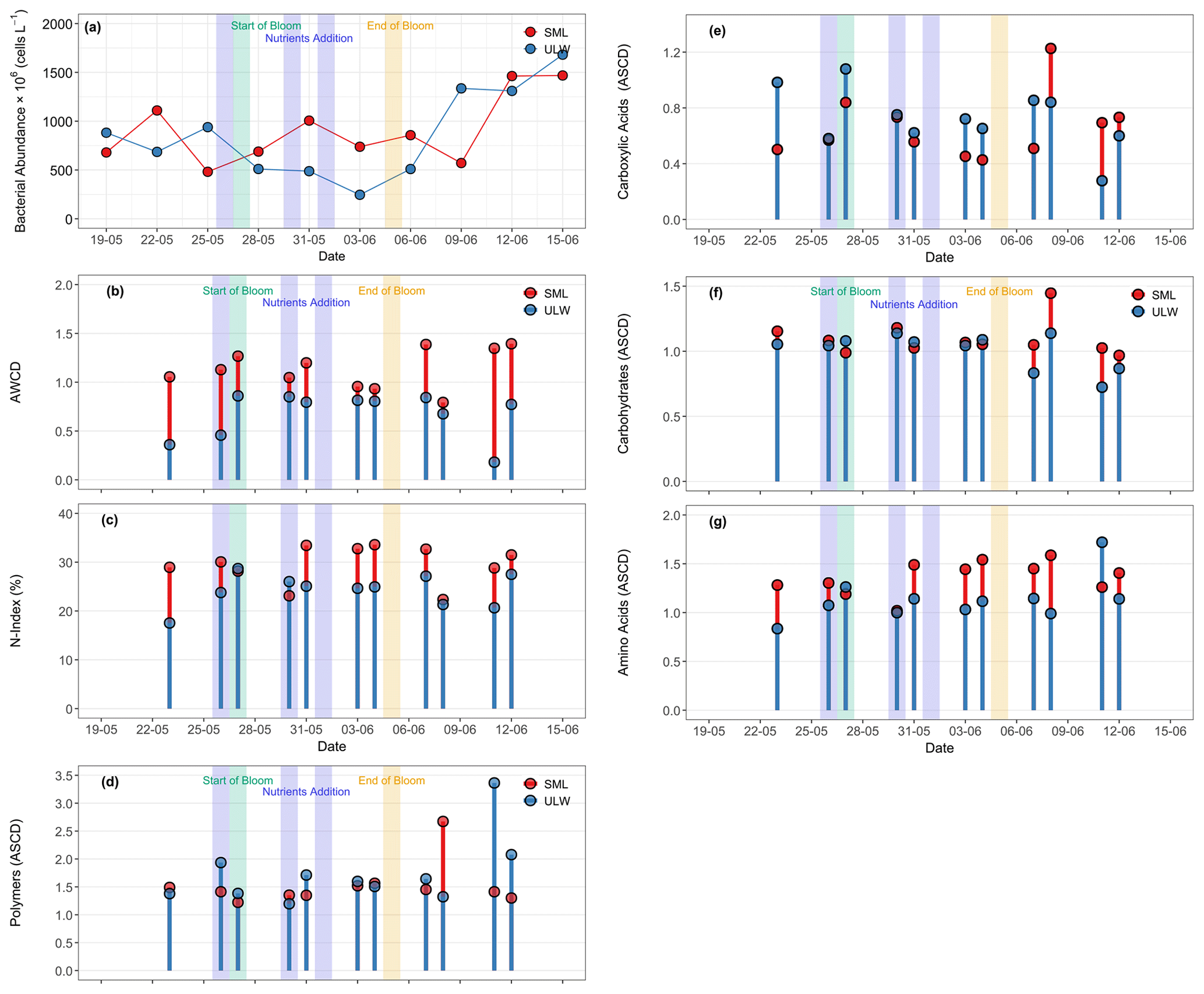
Figure 7 (a) Bacterial abundance (free cells) in the SML (red circles) and ULW (blue circles) during the mesocosm experiment. (b) The average well-color development (AWCD) is defined as the mean absorbance value of Ecoplate at 590 nm. (c) The N-index showing the nitrogen utilisation rate, and the average substrate color development (ASCD) for (d) polymers, (e) carboxylic acids, (f) carbohydrates, and (g) amino acids utilised by bacterial communities in the SML (red stems and circles) and the ULW (blue stems and circles). Please note that for some dates, substrate utilization data were not available (Fig. 7b–g), therefore, the corresponding gaps in the x axis represent days without data.

The carbon utilisation assay (Biolog, Ecoplate) provides insights into the bacterial activities regarding preferred carbon substrates for respiration. The average well-colour development (AWCD) was significantly higher in the SML than in the ULW, possibly due to the formation of slicks during the bloom phase. AWCD ranged from 0.7 to 1.3 (0.9 ± 0.3) in the SML and from 0.1 to 0.8 (0.8 ± 0.3) in the ULW (Fig. 7b). The N-index showed a preference for microbial communities to utilise nitrogen-containing substrates in the SML and the ULW samples. The N-index in the SML ranged from 22.3 % to 33.5 %, while it ranged from 17.5 % to 28.6 % in the ULW (Fig. 7c).

All substrates of the Biolog EcoPlate were grouped into four compound classes: polymers, amino acids, carbohydrates, and carboxylic acids. The average substrate colour development (ASCD) values for individual compounds are provided in Table S2. The average substrate colour development (ASCD) represents the mean color change across all substrates within each group. There were no significant differences in the ASCDs measured in the SML and the ULW samples, indicating equal utilisation of substrate groups in both water layers (Fig. 7d–g). Throughout the mesocosm experiment, the utilisation of substrates in the SML and the ULW remained at similar levels during the pre-bloom, bloom, and post-bloom phases (Fig. 7d–g). The most preferred substrates in both the SML and the ULW were amino acids, with relatively higher utilisation in the SML (ASCD = 3.3 ± 1.3) than in the ULW (ASCD = 2.6 ± 0.4), and the least preferred substrates were carboxylic acids (ASCD = 1.2 ± 0.2 in the SML and 1.0 ± 0.3 in the ULW). Carbohydrates (ASCD = 1.4 ± 0.3 in the SML, 1.1 ± 0.4 in the ULW) and polymers (ASCD = 1.5 ± 0.3 in the SML, 1.7 ± 0.3 in the ULW) were utilised equally in both environments.

3.7 Temporal trends and seasonal heterogeneity in SML and ULW

Based on 60 individual data points (30 dates, 18 May to 16 June, two water layers, the SML and the ULW) of inorganic nutrient samples, we trained the SOM based on a QE of 0.11 and TE of 0.00, and sample data were condensed on a 6 × 6 rectangular grid (Fig. 8a). Hierarchical cluster analysis showed that SOM units were divided into three clusters numbered 1 to 3. (Fig. 8b). Cluster 1 represented the SML and the ULW samples from late May and June. Depending on the similarity and variability in the SML and the ULW samples, cluster 1 was divided into subclusters 1a and 1b (Fig. 8b).

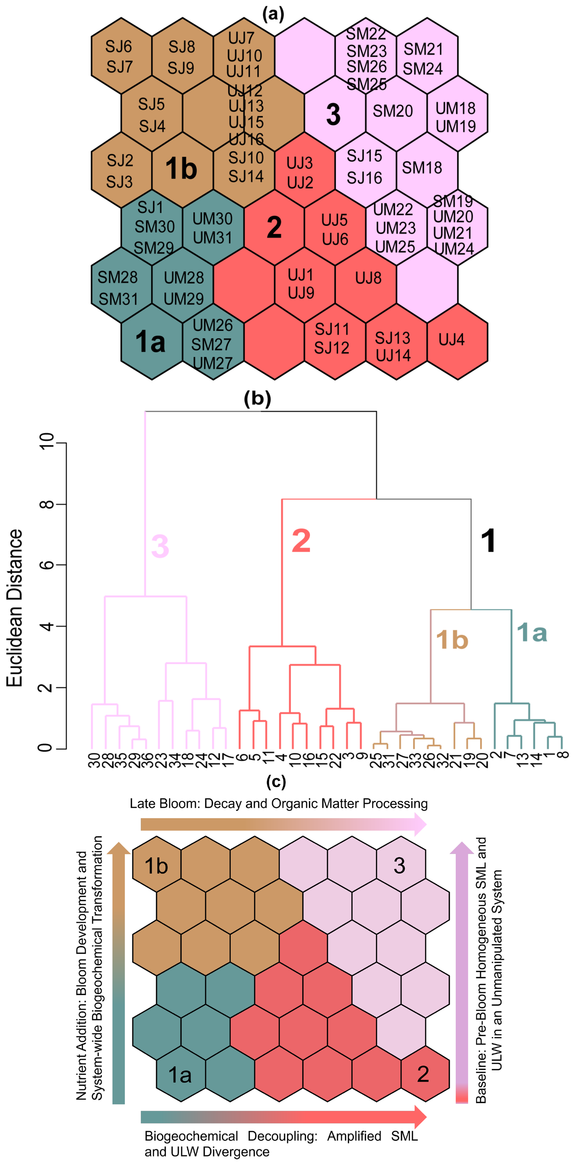
Figure 8 Distribution and visualisation of SML and ULW nutrient samples on the self-organising map (SOM). (a) Acronyms of individual samples are denoted by sampling month (M, May; J, June) and water layers (S, SML; U, ULW). Numbers correspond to the sampling day of the respective month. i.e., SM18 represents the SML sample on 18 May, and UM18 represents the ULW sample on the same date. (b) Hierarchical clustering of the trained SOM nodes, mapped to a dendrogram. Each node on the dendrogram represents the hexagonal cells in the SOM map, i.e., 1 corresponds to neuron 1 in cluster 1. Neuron clustering or counting proceeds from bottom to top and from left to right on the SOM map in panel (a). Different colors and corresponding numbers delineate clusters. (c) Clusters from panel (a) are shown again, illustrating temporal and seasonal variability in SML and ULW nutrient samples. This panel complements panel (a) by presenting the same SOM cluster classification with text labels for easier interpretation, highlighting the temporal progression of the mesocosm experiment and how clusters change across different bloom phases based on nutrient fluctuations and levels over the time of the mesocosm.

Cluster 1a (bluish-green) showed low concentrations of NO${}_{\mathrm{3}}^{-}$ and NO${}_{\mathrm{2}}^{-}$ and high concentrations of Si(OH)₄. Samples in this cluster reflect early bloom conditions and the potential uptake of nutrients by phytoplankton and were assembled at the bottom left side of the SOM map (Fig. 8a). Clusters 1b (brown) and 2 (red) were heterogeneous and representative of samples collected in the second half of the experiment, forming distinct sub-regions on the map (top left and bottom right) with clear segregation of the SML and the ULW samples indicating more divergent nutrient conditions in both water layers. The samples in these clusters had low nutrient concentrations in the SML, but the ULW was characterised by spikes of higher NO${}_{\mathrm{2}}^{-}$ and PO${}_{\mathrm{4}}^{\mathrm{3}-}$ concentrations, likely caused by the remineralisation of OM. Therefore, these samples represent times of late bloom to post-bloom phase and stable nutrient conditions. Cluster 3 (lilac-pink at the top right) was spatially distinct, occupying a consistent region on the SOM map and characterised by high nitrogen, low PO${}_{\mathrm{4}}^{\mathrm{3}-}$ and Si(OH)₄ concentrations, with moderate nutrient variability. This cluster corresponds to the late spring conditions and the transition period from spring to summer prior to nutrient manipulation, specifically during the pre-bloom stage. The overlap of SML and ULW samples suggests homogeneity among the samples, consistent with the fact that these samples were collected during the first phase of the mesocosm experiment when the SML was less distinct (Fig. 8a).

The SOM was applied to obtain a multivariate perspective on bloom development and decline, and it aligned well with bloom dynamics observed through changes in Chl a, POC, and phytoplankton community composition, effectively capturing the key biogeochemical changes over the time of the mesocosm experiment. The spatial configuration of the SOM map revealed distinct temporal segregation of the SML and the ULW nutrients dynamics, associated with phytoplankton bloom progression, collapse and related biogeochemical shifts, during the transition from cooler late-spring to warmer early-summer conditions (mid-May to mid-June) (Fig. 8c). Based on nutrient levels, the progression of biological activity in alignment with phytoplankton growth over time (details described below). Component planes highlight the importance of each input feature and reveal the contribution of individual parameters (nutrient samples in this study) to SOM clusters (Fig. S15).

4 Discussion

Given the complexity of biogeochemical processes in natural environments, studies that integrate in situ field and laboratory measurements at various scales can enhance our understanding of the spatial and temporal variations in the biogeochemical and physical properties of the SML and the ULW. To our knowledge, this is the first multidisciplinary mesocosm study to measure the biogeochemical interactions in the SML and the ULW over a complete phytoplankton bloom succession. Our study revealed distinct patterns of correlations between biogeochemical parameters. The SOM revealed distinct nutrient gradients between the pre-bloom, bloom, and post-bloom phases of the mesocosm. Phytoplankton biomass, estimated through Chl a measurements, and the phytoplankton community responded in accordance with nutrient dynamics. Chl a exhibited a positive correlation with POC and PN. Dissolved organic matter components, such as DOC, TDN, and surfactants, exhibited similar temporal patterns in the SML and the ULW, highlighting the linkage between biological and geochemical processes in both layers. Phytoplankton-driven biological activity, induced by a phytoplankton bloom, resulted in changes in the chemical and physical properties of the SML (Wurl et al., 2016). Variability of biogeochemical parameters was observed to be greater in the SML than in the ULW, indicating its dynamic features due to its direct contact with the atmosphere. However, the strength of the relationships among biogeochemical variables varied with bloom development and was possibly influenced by changes in phytoplankton physiology as suggested by shifts in the POC:Chl a ratio.

4.1 Mesocosms: connecting the field and laboratory studies

Mesocosms are experimental setups designed to replicate elements of the natural environment under controlled conditions. Mesocosm connects field campaigns and laboratory experiments by facilitating the manipulation of desired variables, such as temperature, nutrients, and pH, while ensuring ecological relevance due to their larger scale (Logue et al., 2011). Although mesocosms cannot fully represent the dynamics of oceanic systems, these approaches are suitable for understanding selected oceanic biogeochemical and air–sea exchange processes at a mechanistic level.

To date, most studies characterising the SML biogeochemical dynamics have focused on its biological communities (Cunliffe et al., 2009), the impacts of ocean acidification on the abundance and activity of microorganisms, and changes in the OM composition of the SML (Galgani et al., 2014). Comparatively few studies have also investigated the SML dynamics in the context of environmental changes and their effects on biological and chemical processes (Mustaffa et al., 2017, 2018, 2020b; Barthelmeß et al., 2021). However, these studies were conducted in the field and addressed only individual aspects of the SML rather than its broader interactions (e.g., SML-ULW coupling; biological, chemical, and physical linkages). To our knowledge, no previous studies, either in the field or in mesocosm settings, have examined the coupling of complex, multifaceted biogeochemical processes between the SML and the ULW over the full course of a phytoplankton bloom succession. Thus, this study addresses the gap by presenting the first comprehensive and integrated measurements of biological (phytoplankton biomass and community composition, bacterial abundance and their metabolic profiles), chemical (nutrients and surfactants), and physical (turbidity and solar irradiance) parameters from paired SML and ULW samples, along with their interconnected relationships in a controlled mesocosm setting.

The mesocosm setup enabled us to investigate phytoplankton dynamics throughout the complete phytoplankton bloom succession without external influences such as atmospheric deposition (although some dust deposition occurred, it was unavoidable), wind- and wave-driven mixing, and precipitation. The distinct SOM clustering of nutrient dynamics indicates that nutrient availability was closely linked to the progression of the phytoplankton bloom within the mesocosm. The observed strong positive correlation between POC and PN (r= 0.95), as well as between Chl a and both POC (r= 0.62) and PN (r= 0.60), suggests that phytoplankton remained the dominant source of particulate organic matter (POM) throughout the mesocosm experiment. This observation can have broader implications for other studies that focus on nutrients and carbon dynamics. Enrichment of surfactants in the SML and biofilm formation, as well as the shedding of calcite plates (coccoliths) by Emiliania huxleyi, can lead to high solar reflectivity and albedo, which may potentially affect local energy balance and optical processes relevant to climate interactions (Fig. S16). We highlight key mechanisms regulating OM cycling and biological activity in the SML and the subsequent implications for air–sea interaction in the accompanying special issue.

Our study also has implications for short-term laboratory incubation experiments studying the impact of nutrient enrichment on phytoplankton physiology. The controlled conditions of mesocosms lack the natural variability of the ocean system (e.g., hydrodynamics and grazing that control phytoplankton blooms and bacterial populations), potentially leading to the artificial selection of microbial communities. The short duration of the mesocosm experiment (30 d) may not capture long-term ecological trends, such as interannual variability and delayed microbial responses due to weather changes. The absence of higher trophic interactions could influence observed biogeochemical dynamics and air–sea exchange processes. Further research is needed to address the importance of seasonality and spatial heterogeneity for biological communities, as well as mechanisms governing OM production and transformation. Additionally, by suppressing wind-wave interaction and turbulence, the resulting fully developed surface slicks in the mesocosms can exaggerate the impact of the SML on air–sea exchange processes. All the points make field studies necessary to validate and assess real-world oceanic conditions and feedback mechanisms. Nevertheless, mesocosm studies provide valuable key elements for a mechanistic understanding of complex biogeochemical processes.

4.2 Linking biogeochemical processes in the SML: a mesocosm approach

The mesocosm experiment, conducted over a complete phytoplankton bloom cycle in a controlled setup, showed several consistent patterns and coupling of biogeochemical processes in the SML and the ULW. The results confirmed our study hypothesis that phytoplankton bloom variability influences OM dynamics and that the OM-rich biofilm functions as a biogeochemical reactor, demonstrating the stimulatory effects of nutrient addition on phytoplankton biomass. This contributed to synergistically enhanced OM production in the SML and its subsequent processing by the bacterial community. Our study showed a clear temporal succession of phytoplankton biomass (Chl a, POC, PN) and community shift driven by nutrient dynamics. A previous study (Mustaffa et al., 2020b) has demonstrated that seasonal and temporal variability in nutrient and light availability are crucial factors controlling phytoplankton biomass and species composition in the SML and the ULW. During our mesocosm study, marked differences in nutrient uptake were evident, with a decrease in NO${}_{\mathrm{3}}^{-}$concentration from an average of 7.2 to 0.2 µmol L⁻¹ in the SML. In contrast, NO${}_{\mathrm{3}}^{-}$ concentration in the ULW declined from 7.9 to 0.5 µmol L⁻¹ between the pre-bloom and bloom phases. These changes were reflected in phytoplankton biomass, with an average Chl a increase from 2.2 to 7.3 µg L⁻¹ and a concurrent shift in phytoplankton species composition in the ULW (Fig. 5a–d).

During the pre-bloom phase, nitrogen concentrations were adequate to sustain phytoplankton biomass. As the mesocosm progressed, NO${}_{\mathrm{3}}^{-}$ and NO${}_{\mathrm{2}}^{-}$ concentrations declined, particularly NO${}_{\mathrm{3}}^{-}$, indicating active nitrate uptake by phytoplankton. The low Si(OH)₄ concentrations and high N:P ratios in the ULW (exceeding 100), compared to the Redfield ratio of approximately 16 (Fig. 4e), initially indicated phosphate-limiting conditions during the pre-bloom phase (Ly et al., 2014). After the bloom phase, the N:P ratios dropped to less than 5 in both water layers, suggesting potential co-limitation (Fig. 4e; Moore et al., 2008; Moore et al., 2013), which was further corroborated by the observed decrease in Chl a during the post-bloom phase. The elevated N:P values (> 200) observed during the pre-bloom phase in the mesocosm align with field observations in the North Sea (Grizzetti et al., 2012; Burson et al., 2016). Phosphate limitation (N:P ratios > 16) might have promoted the growth of the coccolithophore Emiliania huxleyi during the pre-bloom phase compared to other phytoplankton groups (Fig. 5b–c), as Emiliania huxleyi is known to adapt to and proliferate efficiently during phosphate-limited conditions (Lessard et al., 2005).

By monitoring Chl a and nutrient concentrations, nutrient addition was conducted to stimulate the development of a phytoplankton bloom. We observed a shift in the phytoplankton community composition. Following the addition of nutrients, the N:P ratio decreased sharply (Fig. 4e). The nutrients addition rapidly elevated Chl a levels, signaling the onset of a significant bloom and an increase in associated biomass. Chl a concentrations, a proxy for phytoplankton biomass, reflected the interplay between nutrient availability and shifts in the phytoplankton community. Two phytoplankton groups dominated the second, larger bloom peak: coccolithophores (Emiliania huxleyi) and diatoms (Cylindrotheca closterium) (Fig. 5c–d). During the final stages of the Emiliania huxleyi bloom, the shedding of coccoliths (3–4 µm, Fig. 5c) increased particle concentrations in the water column, leading to a strong increase in turbidity (Fig. 2b). Thus, towards the end of the experiment, water in the SURF basin took on a milky turquoise appearance due to the accumulation of these calcite plates. These coccoliths, composed of calcium carbonate (calcite), influence the optical properties of seawater due to their high refractive index (Balch, 2018). A higher assemblage of coccoliths during the post-bloom phase may have contributed to increased backscattering of incoming solar irradiance, enhancing light reflectivity and potentially increasing the albedo of the water surface of the mesocosm, consistent with previous findings (Figs. 3b–c and S16) (Tyrrell et al., 1999; Gordon et al., 2009; Neukermans and Fournier, 2018).

Silicate is essential for the growth of diatoms (Krause et al., 2019; Ferderer et al., 2024). The addition and availability of Si(OH)₄ accelerated the growth of the diatom species Cylindrotheca closterium. The decline in overall phytoplankton biomass, as indicated by Chl a, phytoplankton abundance, POC, and PN, during the post-bloom phase coincided with decreasing nutrient levels, especially NO${}_{\mathrm{3}}^{-}$ and Si(OH)₄, emphasising the role of nutrients in sustaining phytoplankton growth and community composition in both the SML and ULW (Mustaffa et al., 2020b). Our mesocosm observations are consistent with previous findings and further highlight that sufficient nutrient availability and ambient light, as well as warm water temperature, promoted swift phytoplankton growth in the ULW (Goldman et al., 1979; Marzetz et al., 2020; Sharoni and Halevy, 2020), leading to phytoplankton biomass accumulation in terms of OM in the SML as supported by DOC and TDN enrichment in the SML (Figs. 6c–d, S13).

The phytoplankton bloom phenology and amplitude observed during our mesocosm study are consistent with established phytoplankton ecological and physiological dynamics, reflecting characteristic succession patterns shaped by nutrient gradients and environmental conditions (Smetacek and Cloern, 2008; Wiltshire et al., 2008; Hyun et al., 2023; Wentzky et al., 2020). The taxonomic shifts in phytoplankton community composition highlight the dominance of different phytoplankton groups over the bloom cycle in response to temporally varying nutrient availability rather than the acclimation of a single group through the mesocosm experiment (González-Gil et al., 2022). These observations highlight that mesocosm experiments can be valuable methods for exploring the complex mechanistic processes happening in natural marine ecosystems. Additionally, these results confirm that our mesocosm facility, SURF, is a suitable design for accurately simulating key biogeochemical processes under controlled conditions.

In addition, the change in Chl a concentration during the bloom phase was accompanied by a rapid increase in POC and PN concentrations in the ULW (Fig. 6e). A positive correlation between POC and PN with Chl a indicated that phytoplankton biomass production was congruent with POM production, consistent with bloom development stages observed during our mesocosm experiment. The POC:Chl a ratio is used to assess the quality and origin of POM (Cifuentes et al., 1988). This ratio is influenced by various factors, including phytoplankton taxonomic composition, species, cell size, and environmental conditions such as light availability, nutrient concentrations, and temperature (Finkel, 2001; Savoye et al., 2003; Putland and Iverson, 2007; Sathyendranath et al., 2009). A POC:Chl a ratio ranging between 40 and 200 is attributed to the dominance of living phytoplankton and freshly produced, highly labile autochthonous POM (Thompson et al., 1992; Cloern et al., 1995; Savoye et al., 2003; Bibi et al., 2020). In contrast, values exceeding 200 indicate an accumulation of detrital material. Throughout our mesocosm experiment, the POC:Chl a ratio remained consistently below 100, indicating a high contribution of living phytoplankton and newly produced POM in situ. This further supports the predominance of phytoplankton-derived POM (Fig. 6f) over the accumulation or introduction of detrital material into the SURF basin during the seawater filling operation on 11 May from the adjacent Jade Bay (Cifuentes et al., 1988; Savoye et al., 2003; Liénart et al., 2016).

Furthermore, the POC:Chl a ratio serves as a metabolic fingerprint of phytoplankton communities, providing valuable insights into their physiological status, growth phases, and responses to nutrient availability and environmental stressors (Geider et al., 1997; Geider et al., 1998). Under nutrient-rich conditions and high growth rates during the bloom phase, phytoplankton synthesised more Chl a, resulting in a lower POC:Chl a ratio (average 14.0) (Jakobsen and Markager, 2016; Behrenfeld et al., 2005). Conversely, during the post-bloom phase, the POC:Chl a ratio was relatively high (average 53.3) due to nutrient stress and increased solar irradiance, as phytoplankton entered senescence or underwent lysis. During this phase, cells allocated more carbon toward structural and storage compounds (e.g. lipids, carbohydrates) rather than Chl a synthesis (Geider, 1987; Wang et al., 2009). In summary, these findings indicate that phytoplankton biomass was the primary source of newly produced POM throughout the mesocosm experiment.

Previous studies have also highlighted phytoplankton blooms as drivers of DOM enrichment in the SML (Wurl et al., 2016; Mustaffa et al., 2017). The transition from peak bloom to decay or decline was marked by a rapid decrease in Chl a, accompanied by a pronounced increase in DOC concentrations. During the post-bloom phase, DOC concentration increased by approximately 1.5-fold, averaging 447 µmol L⁻¹ compared to 278 µmol L⁻¹ observed during the pre-bloom phase. DOC and TDN concentrations in the SML (> 500 µmol L⁻¹ DOC, > 30 µmol L⁻¹ TDN) of our mesocosm study were higher than those previously reported in the field, e.g., in the upwelling regions off the coast of Peru (Engel and Galgani, 2016) or in a controlled wind-wave tunnel experiment in which no distinct phytoplankton bloom occurred (Engel et al., 2018). The pronounced DOC enrichment observed during the mesocosm experiment reflects bloom-driven DOM production during bloom decline, possibly driven by phytoplankton senescence and associated microbial processing. This enrichment in the SML was coupled with increased surfactant concentrations, with EFs reaching up to 15 (Fig. S12). These EFs are substantially higher than those previously reported in field studies, ranging from 0.5 to 7.2 (Wurl et al., 2009, 2011; Sabbaghzadeh et al., 2017). These results also highlight that the composition of the DOM pool, particularly the enrichment of surfactants, plays a more critical role than bulk DOC or TDN concentrations in modulating the physicochemical properties of the air–sea interface.

Active phytoplankton growth during the bloom phase contributed to DOM release (Thornton, 2014), whereas the subsequent senescence and microbial decomposition of that OM amplified surfactant production (Ẑutić et al., 1981). The observed mismatch between Chl a and surfactants suggests physiological stress and senescence of phytoplankton, along with shifts in extracellular organic matter release and microbial processing (Kurata et al., 2016) under less favourable growth conditions, for example, nutrient limitations as the bloom declined (Fig. 4e). The delayed surfactant peak also aligned well with the lifecycle of phytoplankton (low Chl a concentration, high POC:Chl a ratio), suggesting that the here observed surfactant release was linked to phytoplankton bloom decay. Surfactants originate from phytoplankton exudates or cellular lysis, which could be triggered by nutrient or light stress (Ẑutić et al., 1981; Laß et al., 2013) or other environmental causes such as viral or pathogenic interactions.

Increased bacterial abundance (Fig. 7a), high observed surfactant concentrations (up to 1963 µg Teq L⁻¹), and sustained high surface coverage index values above 80 % (Fig. 6a–b) during bloom and post-bloom phases resulted in the distinct slick formation, indicating a biofilm-like habitat (Wurl et al., 2016). The accumulation of surfactants in the SML (slick layer) alters the chemical and physical properties of the SML (Laxague et al., 2024) by trapping more OM. This often results in a thicker SML or gel-like matrix altering the microstructure of SML, e.g., increasing the viscosity and reducing the surface tension (Jarvis et al., 1967) and impacting air–sea gas exchange (Wurl et al., 2016; Pereira et al., 2018; Ribas-Ribas et al., 2018; Mustaffa et al., 2020a).

There was a clear temporal increase in bacterial cell abundance in both the SML and the ULW during the post-bloom phase, consistent with microbial responses to phytoplankton-derived organic matter typically observed during bloom dynamics (Brussaard et al., 1996; Riemann et al., 2000; Buchan et al., 2014). Compared to the bloom phase, the slick or biofilm formed during this period was characterised by higher bacterial cell counts in both water layers (Fig. 7a), indicating a microbial response to elevated DOC concentrations (Fig. 6c). Phytoplankton-derived labile OM increased both the availability and utilisation of organic substrates, as further supported by the low POC:Chl a ratio. The transition from the bloom to post-bloom phase in our mesocosm experiment resulted in changes in both the bioavailability and concentration of released DOM, driven by shifts in phytoplankton species composition and physiological status (e.g., active growth vs. senescence) (Pinhassi et al., 2004; Teeling et al., 2012; Buchan et al., 2014). These changes in DOM composition, in turn, stimulated bacterial growth (Wear et al., 2015; Bunse et al., 2016). The flow-cytometric counts presented here should be regarded as conservative estimates of true bacterial abundance, particularly in the SML, where the high content of organic colloids and exopolymeric particles likely reduced the optical resolution of bacterial signals. This conservative bias, however, does not affect the temporal trends observed, as all samples were processed under identical gating and threshold conditions. The strong correspondence between abundance dynamics and OM indicators (DOC, surfactants, AWCD) therefore reflects genuine microbial responses rather than analytical artefacts.

As previously reported, the accumulation of DOM in the SML and biofilm formation are the hotspots for microbial metabolism and biogeochemical processes (Franklin et al., 2005; Cunliffe et al., 2011; Nakajima et al., 2013; Wurl et al., 2016). Additionally, the high bacterial metabolic activity observed during the post-bloom phase, as indicated by elevated AWCD values in the SML compared to the ULW, suggests that the bacterial community in the SML was utilising more bioavailable OM (Garland and Mills, 1991). This reflects enhanced microbial turnover in the SML, where sustained metabolic activity by the bacterial community actively transformed and retained OM at the air–sea interface (Obernosterer et al., 2008; Cunliffe and Murrell, 2010; Stolle et al., 2011). Consequently, the SML functioned as a biogeochemical reactor, accumulating surfactants and facilitating DOM transformation through the formation of an OM-rich biofilm (Cunliffe et al., 2013; Wurl et al., 2016, and references therein).

During the mesocosm experiment, OM production by phytoplankton was the primary source of carbon, as no organic substances were added. Bacterial metabolic profiles showed that the AWCD and N-Index were consistently higher in the SML than the ULW, coinciding with elevated bacterial abundance in the SML (Fig. 7b–c). A high N-Index percentage or increased nitrogen substrate utilisation may be correlated with phytoplankton-driven PN, as nitrogen-rich compounds, such as amino acids and proteins, are released into the water column (Thornton, 2014). These compounds contribute to the DOM pool, where bacterial communities actively metabolise and transform them. Although substrate utilisation did not show a clear pattern across different bloom stages, the higher amino acid utilisation observed in the SML suggests enhanced in situ production and microbial processing of DOM within this layer (Kuznetsova et al., 2004). The preferential utilisation of amino acids further highlights their role as readily available carbon and nitrogen sources for microbial metabolism (Pérez et al., 2003). These findings highlight the SML as a biologically distinct and dynamic layer, characterised by the enrichment of OM compounds due to surface accumulation and microbial exudation. These enrichments created a nutrient-rich microenvironment that promoted biological activity and microbial metabolism, effectively making the SML a biogeochemical microreactor. Consequently, the SML exhibited distinct biochemical and microbial properties compared to the ULW during the mesocosm experiment.

5 Conclusion

Our findings provide insights into the vital role of phytoplankton-derived OM, possibly originating from both active exudation and cellular lysis, in fueling microbial activity in the SML, highlighting its impact on biogeochemical cycling and air–sea interactions. The observed enrichment of surfactants and DOC in the SML during the post-bloom phase, driven by enhanced biological activity during the bloom, resulted in significant changes in the chemical and physical properties of the SML, including increased PO${}_{\mathrm{4}}^{\mathrm{3}-}$ concentrations, surface coverage, and elevated viscosity due to particle aggregation and the formation of a biofilm-like structure. The strong biological, chemical, and physical coupling, microbial transformation and retention of the OM in SML reinforce its role as a dynamic biogeochemical interface in marine ecosystems. This mesocosm study highlights how both phytoplankton and bacterial processes in the SML influence ocean surface properties. Increased turbidity and albedo during the post-bloom phase, coinciding with SEM-confirmed coccolith shedding, provide experimental evidence that coccolithophore blooms can locally alter ocean surface optics. In addition, biogenic surfactant accumulation can suppress air–sea gas exchange, consistent with previously observed regional and global patterns. Our findings contribute to a deeper understanding of the mechanisms regulating SML biogeochemical variability and highlight the role of phytoplankton and microbial communities in driving surface ocean carbon cycling. A comprehensive understanding of these interactions is crucial for refining climate models to interpret air–sea exchange estimates. Our study provides a groundwork for future investigations into how surface processes influence air–sea interactions and biogeochemical cycling. Since the interactions and links of biogeochemical processes are important and relevant on a global scale for ocean and climate studies, SML's biological, chemical, and physical properties should be integrated into Earth System Models. Developing a comprehensive SML reference model is crucial for understanding its role in the climate system. Future interdisciplinary research focusing on spatial and temporal variability in fields, as well as additional mesocosm studies, is certainly needed to investigate and verify the coupling of biogeochemical processes between the SML and the ULW at regional and global scales, thereby enhancing our understanding of SML dynamics in the ocean-climate system.