Including the invisible: deep depth-integrated chlorophyll estimates from remote sensing may assist in identifying biologically important areas in oligotrophic coastal margins

Surface chlorophyll from satellite remote sensing is a common predictor variable in marine animal habitat studies but fails to capture deep chlorophyll maxima (DCMs) that are unambiguous in persistently stratified water columns. DCMs are also present within the meso-oligotrophic marine environment of Western Australia and have been hypothesised to be an important feature for the growth and maintenance of regional krill populations on which locally endangered pygmy blue whales feed. This study used ∼8500 vertical ocean glider profiles collected between 2008 and 2021 to better understand the broad-scale temporal presence of DCMs and their characteristics in Western Australian waters. Our results show that DCMs are predominantly present from September to April, with a high proportion of biomass maxima within the euphotic zone in September and March. In summer, DCMs deepen and settle below the euphotic zone. The latter results in a balanced presence of biomass and photo-acclimation maxima, placing Western Australian waters in a unique biogeographical biome. In addition, since DCMs in summer contribute over 50 % to water-column-integrated chlorophyll below the euphotic zone, our results are in support of hypotheses regarding the importance of the DCM for local krill and highlight the need to develop methods to include water-column-integrated chlorophyll estimates in habitat models. Linear regression analyses show that this could be achieved through the extension of previously known relationships between surface and water-column-integrated chlorophyll over the euphotic zone to twice the euphotic zone depth (i.e. deep depth-integrated chlorophyll). While using water-column-integrated chlorophyll estimates from satellite remote sensing has its challenges, it is currently the only means to include DCMs in habitat models fitted to large temporal- or spatial-scale animal presence data.

1 Introduction

Phytoplankton are instrumental in providing energy to higher trophic levels of aquatic ecosystems. Their biomass is mostly quantified in terms of chlorophyll-a (hereafter called chlorophyll), from which primary productivity is derived, and areas with potentially high prey availability for higher trophic levels are identified (Huot et al., 2007; Hobday and Hartog, 2014). Indeed, several studies identified chlorophyll as a significant predictor variable of foraging habitat and hot spots for primary consumers (e.g. Schmidt et al., 2012; Hellessey et al., 2020) and higher trophic levels (e.g. Suryan et al., 2012; Palacios et al., 2019; Salgado Kent et al., 2020; Speakman et al., 2020).

While chlorophyll levels can be quantified using several techniques (i.e. visual assessment of ocean colour, spectrophotometry, fluorometry, and chromatography; Parsons and Strickland, 1963; Yentsch and Menzel, 1963; Jeffrey, 1974; Gieskes and Kraay, 1977; Jeffrey et al., 1999), phytoplankton biomass and productivity studies flourished with the launch of the first satellite remote sensing ocean colour mission in 1978 (Hovis et al., 1980; McClain, 2009). Not only has satellite remote sensing generated a near-continuous chlorophyll dataset with high spatial resolution (Groom et al., 2019), the data are also widely accessible, resulting in the inclusion of satellite-derived chlorophyll – almost as a default – in studies aiming to identify crucial marine animal foraging areas. Yet, satellite remote sensing is restricted to the upper water column (2–39 m; Organelli et al., 2017) and likely excludes deep chlorophyll maxima (DCMs; Gordon and McCluney, 1975; Smith, 1981), which may – at least in some areas – be an essential feature to support higher-order foraging efforts (Rennie et al., 2009a; Scott et al., 2010).

DCMs are observed throughout the global oceans, with a year-round and consistent presence in tropical and most subtropical regions (Mignot et al., 2014; Bock et al., 2022; Quartly et al., 2023). Seasonal patterns of occurrence become more evident from temperate to high-latitude regions (Cornec et al., 2021), during which DCMs are present in summer but tend to break down or occur less frequently in winter (e.g. Mignot et al., 2014; Baldry et al., 2020; Bock et al., 2022). In well-studied tropical and temperate regions, DCM formation has been linked to permanent or seasonally stable stratified water conditions (Cornec et al., 2021), with light and nutrient availability driving the formation of true phytoplankton biomass maxima (i.e. deep biomass maxima, DBMs) and deep photo-acclimation maxima (DAMs; Mignot et al., 2014; Cullen, 2015). While DAMs result from an increased chlorophyll-to-carbon ratio because of low-light adaption rather than an increase in transferrable carbon (Steele, 1962, 1964), both DBMs and DAMs may contribute to water column productivity adequately enough to be of relevance to higher trophic levels (e.g. Weston et al., 2005; Fernand et al., 2013; Mignot et al., 2014; Marañón et al., 2021).

The marine habitat of Western Australia is characterised by a cross-shelf gradient in surface chlorophyll values decreasing from winter maxima of $\sim \mathrm{1}\mathrm{mg}{\mathrm{m}}^{-\mathrm{3}}$ along the coast to $\sim \mathrm{0.4}\mathrm{mg}{\mathrm{m}}^{-\mathrm{3}}$ in offshore waters (i.e. >300 m deep; Lourey et al., 2006; Fearns et al., 2007; Hanson et al., 2007a; Koslow et al., 2008). However, surface chlorophyll values vary seasonally and, offshore, generally do not exceed 0.1 mg m⁻³ in summer (Hanson et al., 2005a, b; Lourey et al., 2006; Koslow et al., 2008). These intermittent oligotrophic conditions result from the poleward-flowing Leeuwin Current, which transports warm, low-salinity and low-nutrient water along the continental shelf break (Cresswell and Golding, 1980). Despite seasonal variation in current strength with minimum geostrophic flow in January–February (Feng et al., 2003), the Leeuwin Current generally suppresses nutrient upwelling by strong southwesterly winds that blow in spring and summer (i.e. September–February; Rennie et al., 2006, 2009b). Stratification weakens or may break down in late autumn and winter, which has been linked to an initial deepening of the mixed layer by an intensification of the Leeuwin Current strength (i.e. peak strength in June–July; Feng et al., 2003) and subsequent maintenance of turbulent conditions by northwesterly winter storms and enhanced eddy kinetic energy (Koslow et al., 2008; Rennie et al., 2006).

DCMs form in the vertically stratified water column of Western Australia in summer at a depth between 50 and 120 m offshore, shoaling to the surface or seabed on the continental shelf (Hanson et al., 2005a, 2007a; Twomey et al., 2007; Koslow et al., 2008; Rennie et al., 2009a; Chen et al., 2019). While DCMs tend to break down around the shelf edge in late autumn and winter (Chen et al., 2019), they may persist offshore at shallower depths (15–70 m; Hanson et al., 2005a; Koslow et al., 2008). Previous studies have confirmed that the DCM is often a biomass maximum (Hanson et al., 2005a, 2007a; Rennie et al., 2009a), responsible for 30 %–70 % of total water column productivity (Hanson et al., 2007a). More importantly, the DCM may be a vital feature for Euphausia recurva, the most abundant krill species along the southwest Australian coast, including the Perth Canyon (Sutton and Beckley, 2016). E. recurva, in turn, is the common prey for locally endangered pygmy blue whales (Balaenoptera musculus brevicauda), known to feed around the Perth Canyon head, northern rim, and plateau in waters 300–600 m deep (McCauley et al., 2004; Rennie et al., 2009a) and along the continental shelf break (200 m contour line; Owen et al., 2016) from February to June (peak presence February–March; McCauley et al., 2004; Erbe et al., 2015). Acoustic backscatter data from the Perth Canyon in late summer (February) suggest that krill gather at 300–500 m depth during the day, rising to the DCM at night to feast on phytoplankton prey (Rennie et al., 2009a). Rennie et al. (2009a) highlighted the fact that pygmy blue whales can only be expected to forage in areas where the metabolic gain from foraging supersedes the energy expenditure related to lunge feeding. Based on conductivity, temperature, and depth (CTD) analyses and numerical and phytoplankton studies, the authors hypothesised that the krill population of Western Australia is maintained throughout the year by increased productivity in both winter (related to surface blooms) and summer (related to subsurface blooms near the DCM). Sutton (2015) supported this observation with fatty acid and stable isotope analysis of krill caught in the Perth Canyon in April (i.e. prior to the annual increase in surface phytoplankton in May), which did not reflect a diet of surface phytoplankton. Its apparent significance highlights the need to gain a better understanding of the broad-scale seasonal patterns in DCM formation and potential underlying processes and to consider the inclusion of DCMs in phytoplankton biomass estimates and marine animal habitat models.

While it is known that DCMs form in Western Australian waters, our knowledge of their seasonal presence and characteristics (e.g. DCM depth, type and width, maximum chlorophyll concentration at depth, etc.) is limited to cross-continental shelf time series (e.g. Fearns et al., 2007; Koslow et al., 2008; Chen et al., 2019) and broad-scale temporally restricted analyses (e.g. Hanson et al., 2005a, 2007; Twomey et al., 2007; Thompson et al., 2011). This study used 14 years of ocean glider data to assess broad-scale temporal patterns in water column characteristics, DCM formation, and DCM characteristics in the meso-oligotrophic marine environment of Western Australia, focusing on the area between 27.5 and 33.8° S where the Perth Canyon lies. In addition, while several studies have shown that surface chlorophyll values measurable by satellite remote sensing can estimate water-column-integrated chlorophyll over the euphotic zone (the depth over which photosynthetically active radiation, PAR, decreases to 1 % of its surface value $Z_{\mathrm{1}\mathit{\%}}^{\text{PAR}}$, hereafter referred to as “depth-integrated chlorophyll”; Morel and Berthon, 1989; Uitz et al., 2006; Frolov et al., 2012), these studies were based on samples from open oceanic regions or a regional eutrophic continental margin. We, therefore, assessed whether relationships between surface and water-column-integrated chlorophyll values were similarly present in the waters of Western Australia for potential use in habitat models.

2 Methods

2.1 In situ ocean glider data retrieval

We downloaded in situ ocean glider data from the Australian Ocean Data Network (AODN) portal. Data were collected between 21 June 2008 and 12 July 2022 by the Integrated Marine Observing System Australian National Facility for Ocean Gliders (IMOS-ANFOG; IMOS, 2023) within an area extending from 27.5 to 33.8° S and 109.7 to 115.4° E (Fig. 1). Within this area, the Perth Canyon is located at ∼32° S. Ocean glider missions were conducted each year but with varying intensity between years and concentrated around the continental shelf, shelf break, and deeper waters surrounding the Perth Canyon (see Figs. S1 and S2 in the Supplement for illustrations of temporal and spatial coverage). Consequently, after the filtering process described below and in Sects. 2.2 and 2.3, data were spatially clustered between 31.6 to 32.1° S and 114.9 to 115.3° E, collected between 25 July 2008 and 13 December 2021, and obtained from waters with a mean water depth of 422 m (Fig. 1). All ocean gliders were equipped with a Sea-Bird CTD sensor (models CTD41CP, GPCTD, or SBE_CT) and a Wet Labs ECO Puck optical sensor pack (models BBFL2S, BBFL2VMT, FLBBCDSLK, or FLBBCDSLC), including a fluorometer and backscattering sensor (650–700 nm, 117° centroid angle). All downloaded data were pre-processed and quality-controlled by IMOS, which included the conversion of raw sensor counts into chlorophyll and particle backscatter coefficient (bbp) parameters with instrument-specific calibration coefficients and dark-count values (Mantovanelli and Thomson, 2016; Woo and Gourcuff, 2023). Chlorophyll dark-count values were corrected for any mission with >1 % of negative values (Woo and Gourcuff, 2023). Quality control processes included automatic sensor drift corrections; automatic flagging of impossible location, date, and range values; manual flagging of measurements affected by biofouling or sensor malfunction; and manual flagging of near-surface measurements (<0.5 m). Further data processing was done in MATLAB (Version 2022b; The MathWorks Inc., 2022), while statistical analyses were performed in R and the RStudio statistical software (V4.2.0 and V2023.03.0, respectively; R Core Team, 2022).

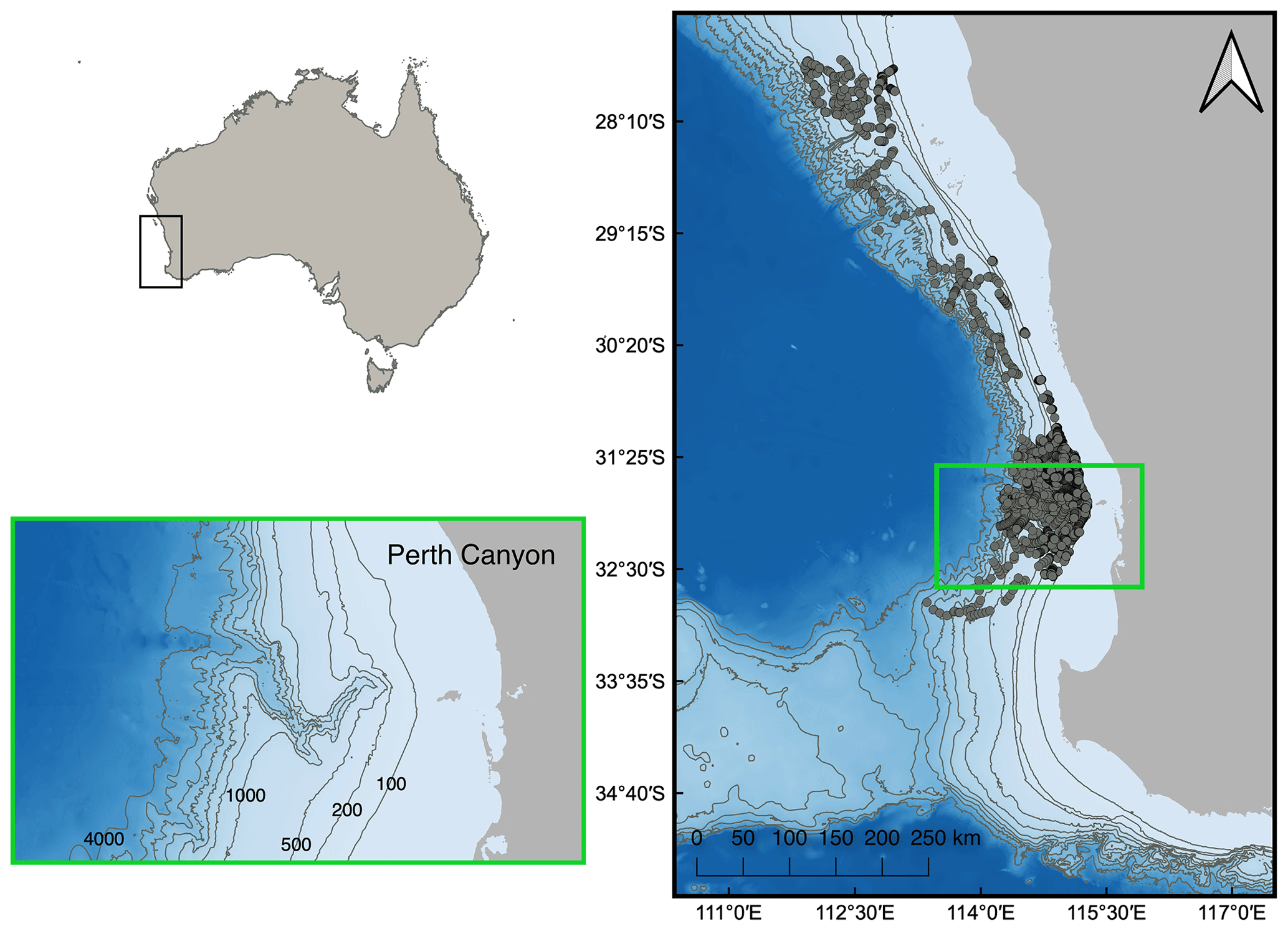
Figure 1 Ocean glider nighttime vertical profile samples (grey circles) collected between the 100 and 3000 m bathymetry contour lines off southwestern Australia, with the Perth Canyon situated at 32° S (within the green square). Bathymetry contour lines delineate isobaths at 100, 200, and 500–4000 m in 500 m increments.

2.2 Ocean glider depth profile extraction

Information extracted from ocean glider data samples included UTC date and time, latitude (decimal degrees, DD), longitude (DD), sampling depth (m), chlorophyll concentration (mg m⁻³), temperature (°C), practical salinity (‰), pressure (dbar), profile phase (i.e. descent, inflexion, or ascent) and, where available, particle backscattering coefficient data (m⁻¹). We filtered ocean glider data based on IMOS quality control flags to retain data points where each variable was flagged as good data, probably good data, value adjusted by the quality control centre, or interpolated value (i.e. flags 1, 2, 5, and 8, respectively; Woo and Gourcuff, 2023). Data were interpolated between each decent and subsequent ascent phase to extract one vertical profile to the deepest recorded depth. Only profiles with at least one observation within the first 10 m of the water column were retained (Uitz et al., 2006). We then calculated the Sun's angle relative to the horizon for each profile with the suncalc R package (Thieurmel and Elmarhraoui, 2022) and removed all profiles obtained with the sun above the horizon (i.e. daytime profiles) from further analyses to avoid underestimating surface chlorophyll concentrations because of non-photochemical quenching (Roesler and Barnard, 2013). Finally, bathymetry data extracted from the Australian bathymetry and topography grid (Whiteway, 2009) were used to omit all samples from waters <100 and >3000 m deep. This was done to ensure that data analyses were focused on a section of the continental margin over which pygmy blue whales have been observed (McCauley et al., 2004; Double et al., 2014; Thums et al., 2022). After this initial filtering process, 21 303 profiles were kept for further processing.

2.3 Temporal patterns in water column conditions

The prevalence of DCMs and the relationship between surface and depth-integrated chlorophyll concentrations differ between mixed and stratified water columns (Morel and Berthon, 1989; Uitz et al., 2006; Cullen, 2015). We, therefore, split profiles between mixed and stratified water conditions based on the euphotic zone depth (i.e. $Z_{\text{eu}}=Z_{\mathrm{1}\mathit{\%}}^{\text{PAR}}$; see Table 1 for a list of symbols) and mixed-layer depth (MLD) as positive values below the surface. Following Uitz et al. (2006), we classified waters as mixed when Z_eu<MLD and stratified when Z_eu>MLD. The euphotic zone depth for each profile was derived from the vertical chlorophyll distribution by progressive trapezoidal integration of chlorophyll over depth (Z; Morel and Berthon, 1989). For each sampling depth (Z_i), we converted depth-integrated chlorophyll concentrations to euphotic zone depth using formulae from Morel and Maritorena (2001) until Z_eu<Z_i (Morel and Berthon, 1989). The exact euphotic zone depth was then calculated by interpolating Z_eu between Z_i and Z_i−1 to find where Z equalled Z_eu (Morel and Berthon, 1989). Profiles that did not reach the euphotic zone depth were discarded, leaving 8486 profiles for statistical analyses.

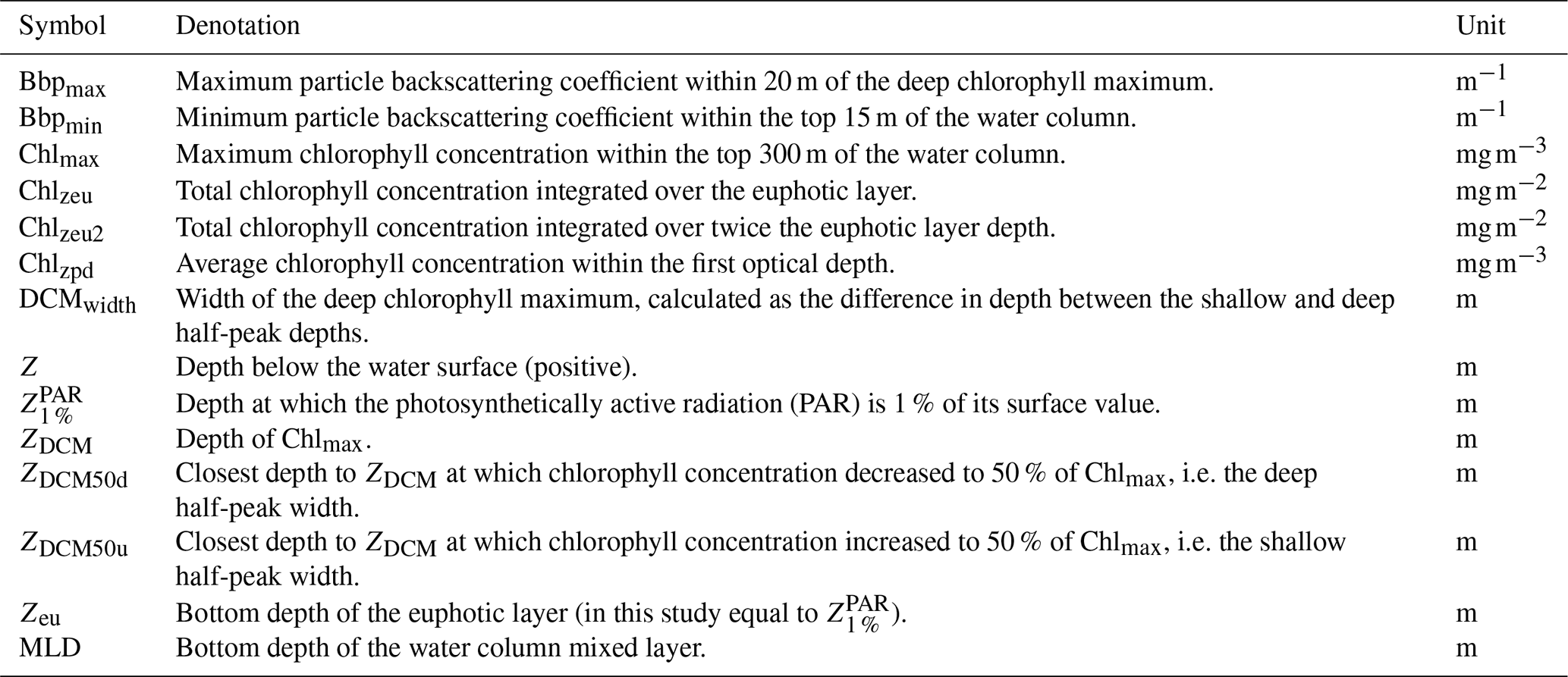
Table 1 List of symbols used in this study and their denotation.

Raw temperature, salinity, and pressure data were converted to potential temperature and density values with the Gibbs-SeaWater (GSW) Oceanographic Toolbox (IOC et al., 2010; McDougall and Barker, 2020) to calculate the mixed-layer depth. Here, we define the mixed-layer depth as the first depth at which either the potential temperature differed by 0.2 °C from the reference potential temperature or the potential density exceeded the reference potential density by 0.03 kg m⁻³, with samples taken at a 10 m depth as reference values (de Boyer Montégut et al., 2004; Boettger et al., 2018).

2.4 Temporal patterns in DCM presence, classification, and characteristics

Cornec et al. (2021) identified values and depths of maximum chlorophyll and particle backscatter coefficient data from smoothed vertical profiles before locating the nearest equivalent maximum chlorophyll (Chl_max) and particle backscatter coefficient (Bbp_max) on the unsmoothed profiles. Maxima values from the unsmoothed profiles were then compared to values within the top 15 m to identify whether a DCM was present (i.e. Chl_max exceeded twice the median chlorophyll concentration over the top 15 m) and whether a DCM was a DBM (i.e. Bbp_max exceeded 1.3 times the minimum particle backscattering coefficient in the top 15 m) or a DAM. Our methods followed those of Cornec et al. (2021), with a minor modification to the smoothing process. Chlorophyll profiles were smoothed with a 5-, 7-, or 11-point moving median corresponding to median profile depth resolutions of ≥3, <3 but >1, and ≤1 m, respectively (Schmechtig et al., 2023). Particle backscatter coefficient profiles were smoothed with an 11-point moving median, followed by an 11-point moving mean. The depth of Chl_max (Z_dcm; DCM peak depth), shallow half-peak depth (Z_dcm50u), and deep half-peak depth (Z_dcm50d) were also extracted. The DCM width (DCM_width) was calculated as the depth range between the shallow and deep half-peak depths (i.e. Z_dcm50d−Z_dcm50u). Trends in the position of the DCM peak and width relative to the euphotic zone were assessed by calculating their relative positions as ${\text{Chl}}_{\text{max}}/Z_{\text{eu}}$ and $Z_{\text{dcm50d}}/Z_{\text{eu}}$, respectively, where values <1 were indicative of a peak chlorophyll value or a full half-peak width within the euphotic zone.

2.5 Relationships between surface and water-column-integrated chlorophyll

Relationships between surface and water-column-integrated chlorophyll concentrations were assessed based on methods described in earlier publications (Morel and Berthon, 1989; Uitz et al., 2006; Frolov et al., 2012). We calculated surface chlorophyll values – assumed to be measurable by satellite – as the average chlorophyll concentration over the first optical depth (i.e. Chl_zpd; Uitz et al., 2006), where the first optical depth refers to $Z_{\text{eu}}/\mathrm{4.6}$ (Gordon and McCluney, 1975). Since $Z_{\mathrm{1}\mathit{\%}}^{\text{PAR}}$ may underestimate the biological compensation depth at which the rate of photosynthesis equals that of autotrophic respiration and, thus, the depth of the productive layer, we integrated chlorophyll concentrations via trapezoidal integration over the euphotic zone (i.e. depth-integrated chlorophyll; Chl_zeu) and where possible, twice the euphotic zone depth (hereafter referred to as “deep depth-integrated chlorophyll”; Chl_zeu2). The latter differs from that of Uitz et al. (2006), who integrated chlorophyll over a maximum of one-and-a-half times the euphotic zone depth because preliminary analysis indicated that 34.8 % of DCM half-peak widths extended beyond that limit (see Fig. S3 in the Supplement for a DCM full-width inclusion curve).

Relationships were quantified using linear regression analyses on log ₁₀ transformed data, conducted separately for mixed and stratified water conditions. Previous publications used two regression lines to quantify the relationship in stratified waters because of a change in slope at surface chlorophyll values of $\sim \mathrm{1}\mathrm{mg}{\mathrm{m}}^{-\mathrm{3}}$ (Morel and Berthon, 1989; Uitz et al., 2006; Frolov et al., 2012). While preliminary data analysis revealed a similar change in slope in this study, the change appeared to be seasonal and related to a change in the shape of vertical chlorophyll profiles from ones with low surface chlorophyll values and a pronounced DCM to ones with higher surface chlorophyll values without a DCM (Fig. 2). Thus, we carried out one regression analysis for stratified water conditions from September until April and one for stratified water conditions from May until August. For brevity, the two seasons will be referred to as summer–transition and midwinter, respectively. We evaluated all models with the mean absolute error (MAE) and bias metrics because of tailed distributions in model residual plots (Chai and Draxler, 2014; Seegers et al., 2018; Hodson, 2022). Both metrics were transformed from linear to multiplicative values for ease of interpretation (Seegers et al., 2018). The slope and intercept of the linear regression were converted into a power-law regression to describe the non-linear relationship between non-transformed surface and water-column-integrated chlorophyll values.

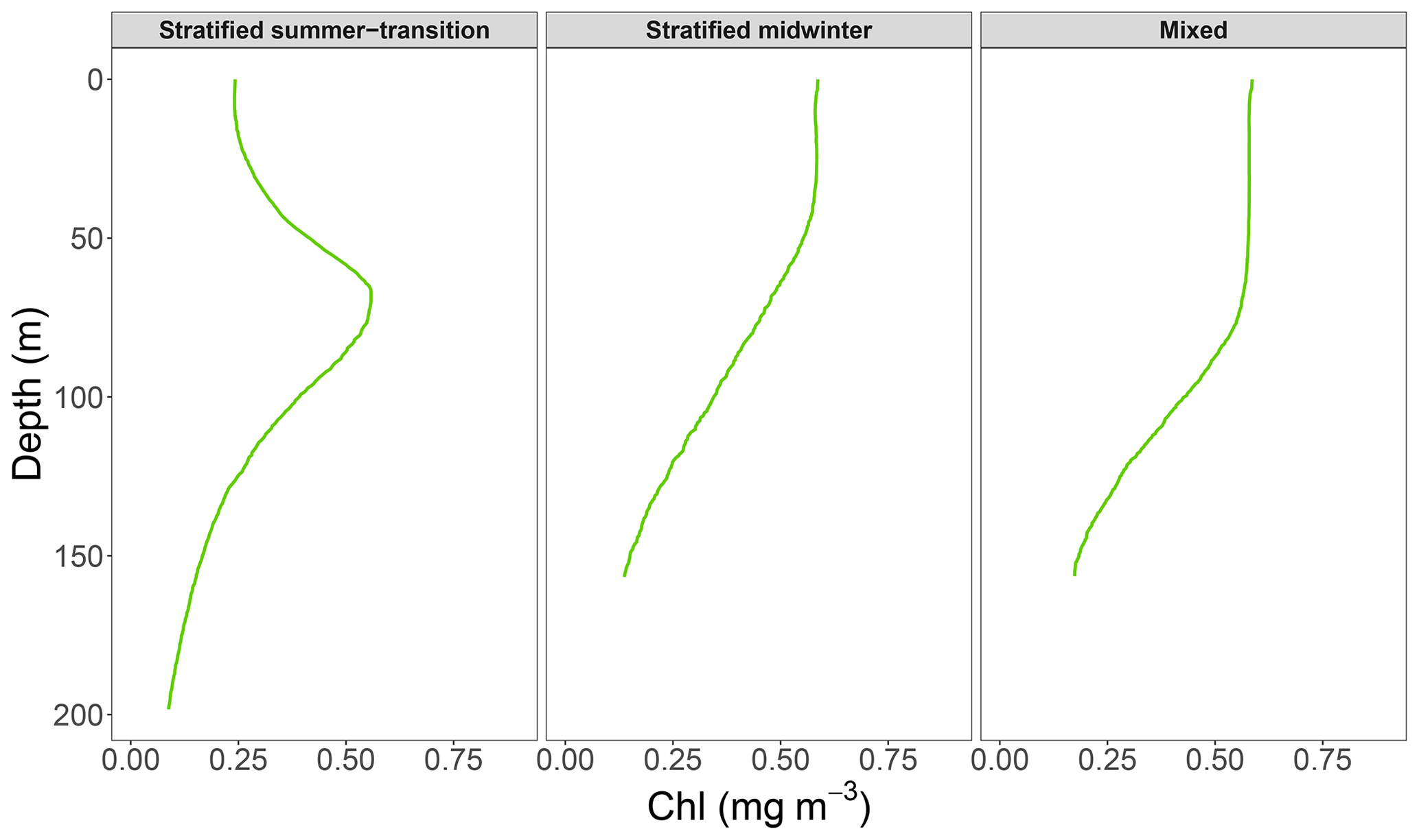
Figure 2 Median vertical chlorophyll profiles for the (a) stratified summer-transition (September–April), (b) stratified midwinter (May–August), and (c) mixed-water conditions.

3 Results

3.1 Temporal patterns in water column conditions

We extracted 5543 and 2943 profiles from stratified and mixed water conditions, respectively. Stratified water conditions dominated over the warm late-spring, summer, and early-autumn months (October–March; ≥85 % of profiles), declining to <39 % over May–July when mixed water conditions prevailed (Fig. 3b). Transition conditions were present in April, August, and September, with an approximate 50:50 occurrence of stratified and mixed water conditions. The change in the prevailing water condition was predominantly caused by a deepening of the median mixed-layer depth from 30.5 m (IQR 21.0 m) in February to 65.5 m (IQR 51.0 m) in July (Fig. 3c). In contrast, the euphotic zone depth moved closer to the surface from a median of 73.3 m (IQR 12.5 m) in December to 46.3 m (IQR 10.9 m) in May (Fig. 3c).

Figure 3 Number of profiles extracted for each month (black bars in a) overlain with the number of profiles for which the mixed-layer depth (MLD) was reached (grey bars in a). For each month, the proportion of vertical profiles extracted from mixed (solid pink line) and stratified (solid blue line) water conditions is provided in panel (b), along with the proportion of profiles characterised by a DCM (dashed red line in b) and the seasonal change in median (with the 25th and 75th quartiles as shaded areas) euphotic zone (Z_eu) and mixed-layer depth (c). Panel (d) shows the monthly median vertical chlorophyll profiles.

3.2 Temporal patterns in DCM presence, classification, and characteristics

DCMs were predominantly found in stratified water conditions (56.5 % of stratified profiles vs. 3.3 % of mixed profiles; 3133$/$5543 vs. 97$/$2943); thus, the seasonal presence of DCMs followed the seasonal pattern in water column stratification, with a peak presence from October until March (>64 %; Fig. 3b). However, despite stratification in at least 30 % of profiles in winter, DCMs practically disappeared in May–July (<3 % of profiles; Fig. 3b), changing the vertical chlorophyll distribution into a sigmoid shape (Fig. 3d). Overall, DCMs formed between the surface and 167.1 m deep, at a median depth of 75.3 m (IQR 29.3 m). However, median DCM depths varied seasonally, with shallowing events in January (68.6 m; IQR 19.8 m), April (38.6 m; IQR 19.7 m), and September (65.4 m; IQR 38.4 m). Seasonal maxima depths were reached in February (75.2 m; IQR 32.3 m), July (95.9 m; IQR 130.8 m), and December (83.0 m; IQR 31.1 m), although DCMs in July appeared to form either close to the surface or at great depths (Fig. 4a). From June until December, there was an overall deepening trend during which the chlorophyll maximum moved further away from the mixed layer while remaining at an approximate constant relative distance from the euphotic zone (∼1.1 times the euphotic zone depth; Fig. 4b). Median DCM half-peak widths concurrently narrowed (Fig. 4c), while the maximum chlorophyll concentration showed a modest increase (Fig. 4d). The exception to this trend was a brief shallowing to just above the bottom of the euphotic zone in September (0.99; IQR 0.45), characterised by a rapid increase in peak chlorophyll levels at the DCM. A contrasting shallowing trend can be discerned from December until April, positioning the chlorophyll maximum at a nearly constant relative distance from the bottom of the mixed layer (∼2.0 times the mixed-layer depth) but elevating the chlorophyll maximum to well within the euphotic zone in April (0.75; IQR 0.19). Despite this shallowing trend, DCMs remained of a similar width as in December, and modest intensification of the chlorophyll maximum continued until a sudden deepening, widening, and weakening of the DCM in May.

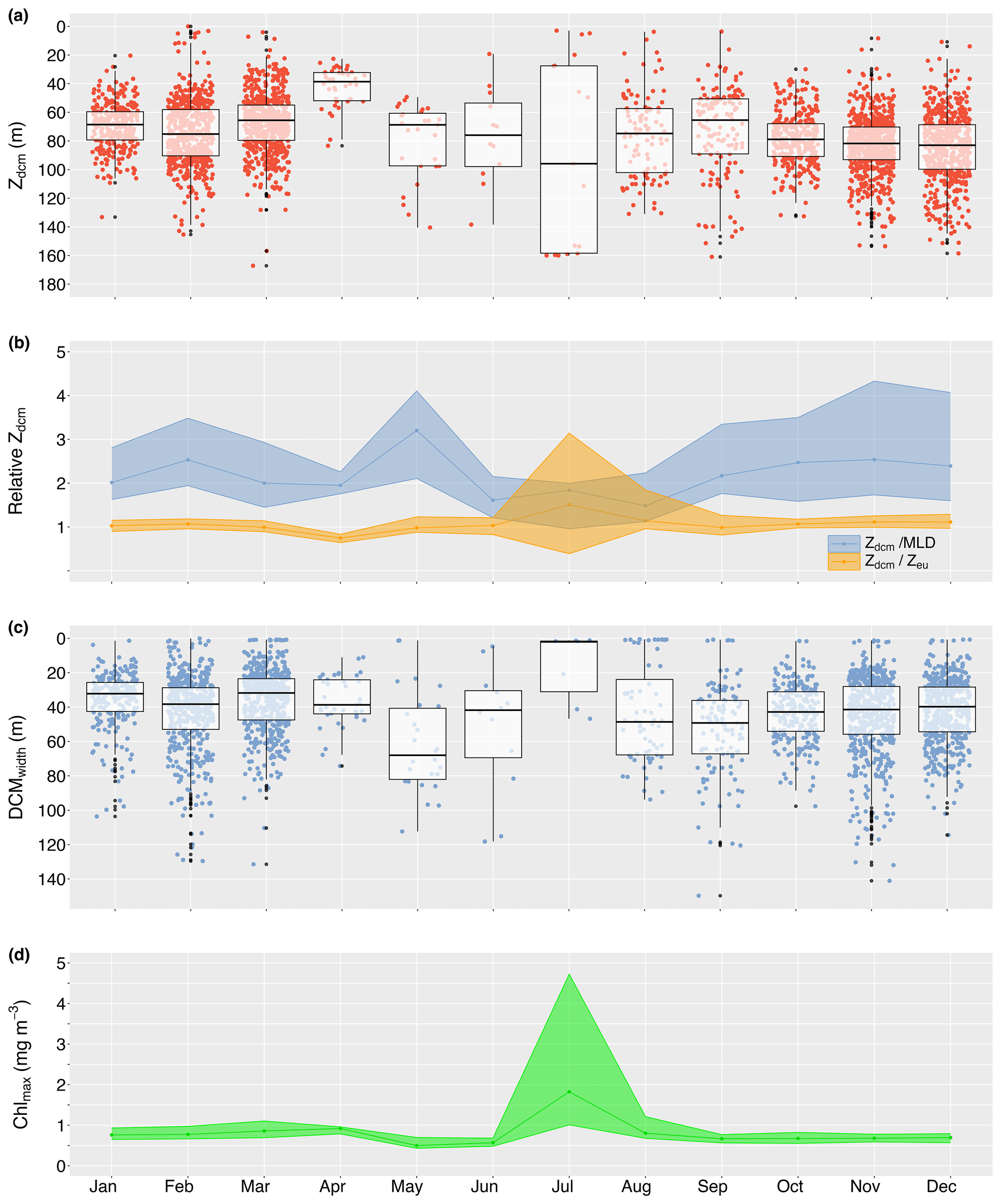
Figure 4 Median monthly true DCM depth (Z_dcm; a) and relative depth in relation to the bottom of the mixed-layer ($Z_{\text{dcm}}/\text{MLD}$; b) and euphotic zone ($Z_{\text{dcm}}/Z_{\text{eu}}$; b). Panels (c) and (d) reflect the seasonal change in DCM width and maximum chlorophyll concentration at the DCM. The shaded ribbons in panels (b) and (d) indicate the 25th and 75th quartiles.

Particle backscatter data were available for 1551 profiles, of which 95.8 % were collected in September–March (1487$/$1551). Over this time, the proportion of DBMs gradually declined from 69.7 % in September to 46.2 % in January, which is also shown by a disproportional change in maximum particle backscatter and chlorophyll amplitudes (see Fig. S4 in the Supplement for temporal patterns in DBM and DAM characteristics). As the DCM became shallower in late summer, DBMs became more prevalent again, with a peak presence in March (81 %). However, the sudden deepening, widening, and weakening of the DCM in May pivoted DCM-type classifications to a prevalence of DAMs (70 %), which generally dominated in winter (i.e. 66.1 %). Overall, DAMs were moderately weaker, wider, and positioned deeper in the water column than DBMs, yet the position of the maximum chlorophyll relative to the euphotic zone depth remained within 1.2 times the euphotic zone depth.

3.3 Relationships between surface and water-column-integrated chlorophyll

Surface chlorophyll concentrations (Chl_zpd) ranged between 0.04 and 1.58 mg m⁻³ (median 0.44 mg m⁻³, IQR 0.38 mg m⁻³), with marked seasonal changes (Fig. 5a). Monthly median surface chlorophyll values peaked in May (0.77 mg m⁻³, IQR 0.37 mg m⁻³; Fig. 5a), remained $>\mathrm{0.5}\mathrm{mg}{\mathrm{m}}^{-\mathrm{3}}$ in winter, but rapidly decreased over September to minimum median levels of $\sim \mathrm{0.20}\mathrm{mg}{\mathrm{m}}^{-\mathrm{3}}$ in November and December. A subsequent increase can be discerned for January (0.27 mg m⁻³, IQR 0.13 mg m⁻³), although values remained $<\mathrm{0.33}\mathrm{mg}{\mathrm{m}}^{-\mathrm{3}}$ throughout early autumn before rapidly transitioning to peak levels over April. A similar seasonal pattern was present in depth-integrated chlorophyll values, albeit less pronounced (Chl_zeu; Fig. 5b). Interestingly, monthly median deep depth-integrated chlorophyll similarly peaked in May (Chl_zeu2; 62.2 mg m⁻², IQR 17.3 mg m⁻²), but a secondary increase can be discerned in August (53.9 mg m⁻², IQR 14.1 mg m⁻²), after which levels declined less rapidly to the seasonal minimum in December (48.7 mg m⁻², IQR 9.2 mg m⁻²; Fig. 5b). In January, deep depth-integrated chlorophyll increased more evidently than depth-integrated values and subsequently remained relatively constant from February until April (i.e. $\sim \mathrm{52.0}\mathrm{mg}{\mathrm{m}}^{-\mathrm{2}}$). Overall, chlorophyll below the euphotic zone depth accounted for 50 %–60 % of deep depth-integrated values from October until March, declining to a minimum of 44 % in April, May, and July.

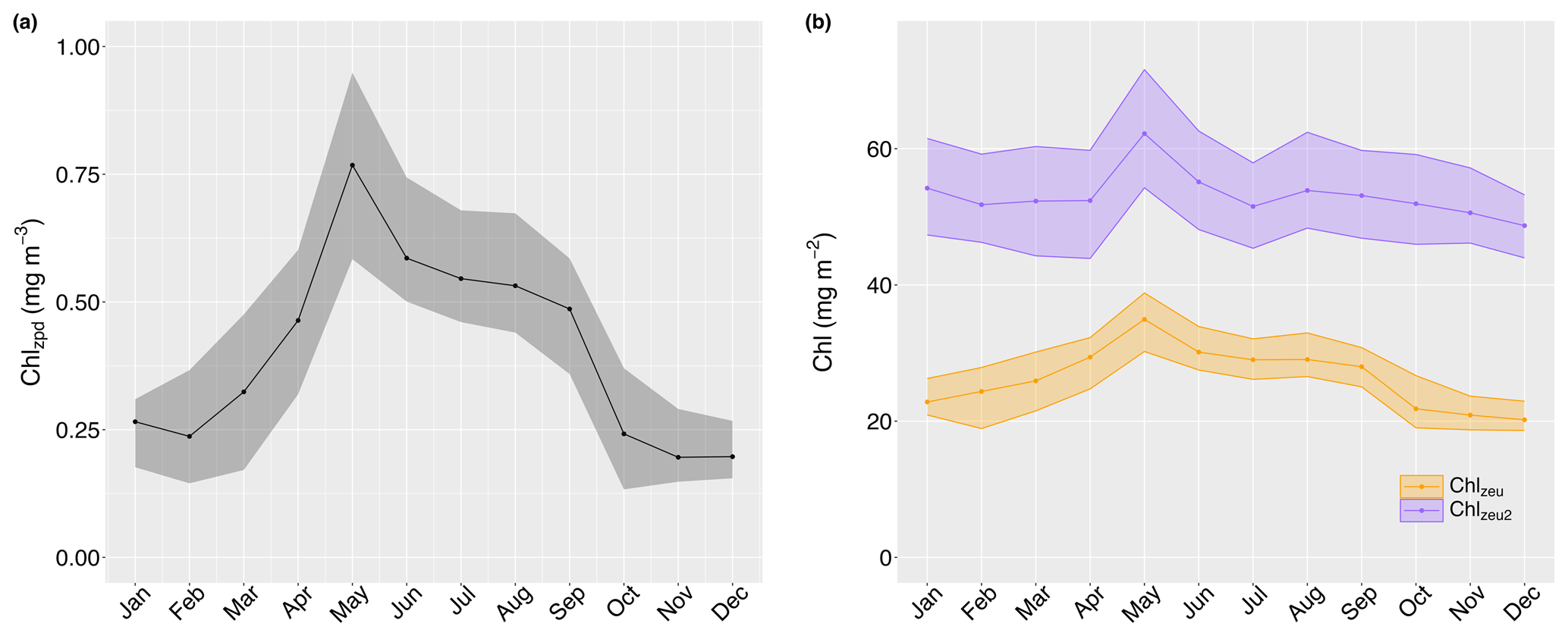
Figure 5 Monthly median surface (Chl_zpd; a), depth-integrated (Chl_zeu; solid orange line in b), and deep depth-integrated (Chl_zeu2; solid purple line in b) chlorophyll values with their 25th and 75th quartiles as shaded areas.

Profiles collected from stratified water conditions in summer-transition months showed a significant linear relationship between surface and depth-integrated chlorophyll concentrations (R²=0.72, $F_{(\mathrm{1},\mathrm{4002})}=\mathrm{10}\mathrm{420}$, p<0.001; Fig. 6a). A stronger relationship with a steeper slope and less scatter was seen for the stratified midwinter months (R²=0.87, $F_{(\mathrm{1},\mathrm{1533})}=\mathrm{10}\mathrm{080}$, p<0.001; Fig. 6b) and mixed water columns (R²=0.97, $F_{(\mathrm{1},\mathrm{2940})}=\mathrm{90}\mathrm{400}$, p<0.001; Fig. 6c). Scatter around the regression line resulted from the presence of DCMs, with no apparent difference between the contribution of DBMs and DAMs. Thus, the mean relative error was highest (8.9 %; MAE=1.089) for estimates of observed depth-integrated chlorophyll from surface chlorophyll values under stratified water conditions in summer-transition months, when DCMs were more common. Under stratified water conditions in winter and mixed water conditions, the mean relative error reduced to 5.6 % and 1.7 %, respectively (i.e. MAE = 1.056 and 1.017, respectively). Scatter in the data increased for deep depth-integrated values, resulting in a weak linear relationship in stratified summer-transition months (R²=0.15, $F_{(\mathrm{1},\mathrm{2729})}=\mathrm{498.5}$, p<0.001; Fig. 6d) and a moderate relationship in both stratified midwinter months (R²=0.48, $F_{(\mathrm{1},\mathrm{1351})}=\mathrm{1232}$, p<0.001; Fig. 6e) and mixed water columns (R²=0.63, $F_{(\mathrm{1},\mathrm{2512})}=\mathrm{4239}$, p<0.001; Fig. 6f). As a result, mean relative errors increased to 15.7 %, 15.2 %, and 8.6 %, respectively. All derived non-linear relationships are summarised in Table 2.

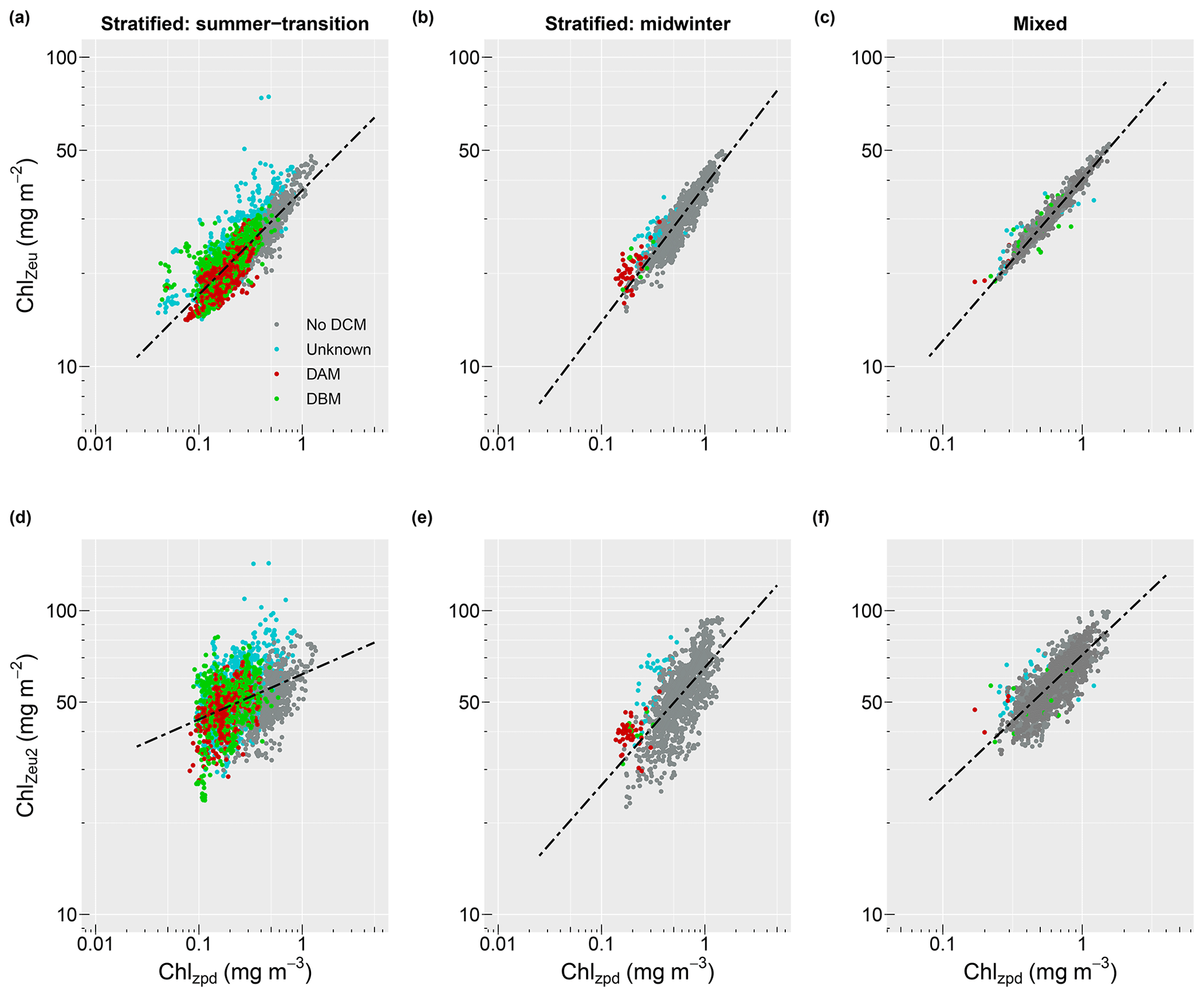
Figure 6 Relationship between surface (Chl_zpd) and depth-integrated (Chl_zeu) vs. deep depth-integrated (Chl_zeu2) chlorophyll values for stratified water conditions in summer-transition months (i.e. September–April; a, d), stratified water conditions in midwinter months (i.e. May–August; b, e), and mixed water conditions (c, f). Dots are coloured according to whether a DCM was absent (grey), present but of unknown type (turquoise), a DBM (green), or a DAM (dark red). Black dashed lines indicate the derived regression lines. Note the change in y axis range between panels (a–c) and (d–f) and the change in x axis range between stratified (Z_eu>MLD) and mixed water (Z_eu<MLD) conditions.

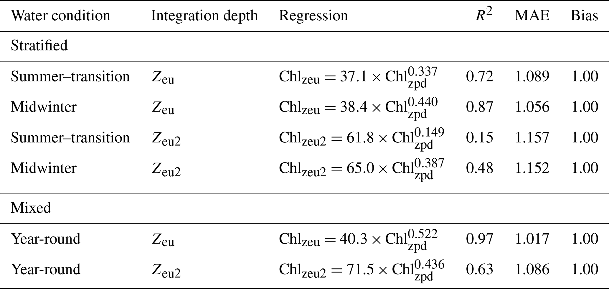
Table 2 Summary of non-linear relationships between surface (Chl_zpd) and depth-integrated (Chlq_zeu) vs. deep depth-integrated (Chl_zeu2) chlorophyll under stratified and mixed water conditions. Relationships in stratified waters are given for both summer–transition (September–April) and midwinter months (May–August).

4 Discussion

4.1 Seasonality in water column characteristics and DCM formation

The marine environment of Western Australia is governed by the warm, poleward-flowing Leeuwin Current of tropical origin, with signatures from the higher salinity subtropical Indian central waters (Waite et al., 2007; Woo and Pattiaratchi, 2008). Because of generally low surface chlorophyll values beyond the continental shelf and a broad winter increase in surface chlorophyll from May until September, Western Australian waters are often labelled as oligotrophic (e.g. Twomey et al., 2007; Feng et al., 2009; Rennie et al., 2009a; Chen et al., 2019), with a surface productivity regime comparable to subtropical gyres (Koslow et al., 2008). These subtropical areas are characterised by either permanently stratified water columns or brief (∼1 month) mixing periods, resulting in a (near-)permanent DCM presence (Mignot et al., 2014; Quartly et al., 2023). Our results show that stratification in winter (May–August) is intermittent and that DCM formation is the exception rather than the norm (i.e. <3 % of profiles). The disappearance of DCMs from vertical profiles corresponds to a period of intense Leeuwin Current strength, which is known to weaken stratification (i.e. May–July; Koslow et al., 2008; Feng et al., 2003, 2009). In addition, northwesterly downwelling-favourable storms ($\text{wind speeds}>\mathrm{15}\mathrm{m}{\mathrm{s}}^{-\mathrm{1}}$; most frequent in June–August) and concomitant surface cooling mix the water column down to 200 m depth, breaking down the stratified layer and the DCM (Rennie et al., 2006; Chen et al., 2020). While re-stratification has been shown to occur during subsequently calm post-storm southwesterly winds ($\text{wind speeds}<\mathrm{7}\mathrm{m}{\mathrm{s}}^{-\mathrm{1}}$; Rennie et al., 2006), our data reveal that these re-stratification periods often do not persist long enough for DCMs to reform. This is likely because of the additive effect of increased eddy kinetic energy, which peaks in July (Feng et al., 2005). Warm-core eddies, in particular, are frequent in late autumn and winter between 28 and 31° S, generating well-mixed layers extending beyond the euphotic zone depth (Thompson et al., 2007; Waite et al., 2007). Consequently, our area experiences a mixing period of approximately 3 months, which is more comparable to the duration of mixing periods in the Mediterranean (Mignot et al., 2014; Barbieux et al., 2019) and oligotrophic subtropical open oceans (Chiswell et al., 2022).

4.2 DCM characteristics

Leeuwin Current strength significantly drops (Feng et al., 2003), and winter storms settle in September (Pearce et al., 2015), which is when stratified water columns return. However, eddy kinetic energy remains persistent (Feng et al., 2009). Warm-core eddies have been hypothesised to facilitate phytoplankton blooms through the injection of nitrogen into surface waters (Lourey et al., 2013) and the formation of a shallow nutricline (∼60 m depth) under a relaxed Leeuwin Current after eddies detach from the shelf (Koslow et al., 2008). Our data support this hypothesis, with a reappearance of DCMs, which were predominantly biomass maxima, in September at a median depth of 65.4 m. The subsequently observed deepening of the DCM through spring and summer is common for oligotrophic regions (Mignot et al., 2014; Chiswell et al., 2022). In our study area, as the DCM deepened and intensified, backscatter vertical profiles changed disproportional to chlorophyll vertical profiles, reflecting the decreased occurrence of DBMs until biomass and photo-acclimation maxima occurred in approximately equal proportions from December until February. DCM formation is always at least in part caused by photo-acclimation of phytoplankton to low-light conditions (Cullen, 2015), but deep DCMs in summer may approach the nutricline, allowing for phytoplankton growth and, thus, DBM formation (Mignot et al., 2014). DCM settlement within a nearly constant distance from the euphotic zone depth (i.e. ∼1.1 times the euphotic zone depth), regardless of DCM type, suggests photo-acclimation processes in response to light limitation as the main driver of DCM formation from September until late summer. However, the balanced presence of photo-acclimation and biomass maxima in our study indicates that access to nutrients is indeed available throughout summer. These findings fit the equal occurrence of upwelling and downwelling days detected in temperature time series by Rennie et al. (2006) and the positioning of the summer DCM just above the nutricline in earlier studies (e.g. Hanson et al., 2007a, b; Koslow et al., 2008). In addition, Rennie et al. (2006) detected a concentration of upwelling events in late February–early March, which temporally matches an initial weakening of stratification as the Leeuwin Current starts to intensify (Feng et al., 2003; Koslow et al., 2008) and, in our study, matches the timing of DCM shallowing and intensification and a rapid increase in biomass maxima. Thus, while the DCM formation is first-order light-driven, nutrient limitation in the upper water column in autumn and at depth in summer likely drives the balance between biomass and photo-acclimation maxima until upwelling and increased water turbidity potentially synergistically increase nutrient levels within the bottom layer of the euphotic zone. Our results suggest that DCMs in Western Australian waters form via bio-optical mechanisms that match neither pattern observed in subtropical oceanic (Mignot et al., 2014; Chiswell et al., 2022; Quartly et al., 2023) and more productive temperate regions (Mignot et al., 2014; Barbieux et al., 2019) but instead are similar to the mid-Mediterranean Sea, which forms a transition between the meso-oligotrophic western and oligotrophic eastern basins (Barbieux et al., 2019). However, a broad-scale long-term study, including nutrient and irradiance parameters, is required to elucidate our hypothesis.

4.3 Water-column-integrated productivity

Seasonal surface chlorophyll fluctuations followed the commonly observed pattern of a winter surface chlorophyll increase, albeit with our observed peak in May preceding the June–July winter bloom previously described by Lourey et al. (2006) and Koslow et al. (2008). This shift could be related to changing trends in environmental and oceanographic drivers. Long-term data series from IMOS national reference stations around Australia have shown, for example, that mixed-layer and euphotic zone depth follow an overall deepening trend from 2008 to 2018 by 1.02 and 1.7 m yr⁻¹, respectively (van Ruth et al., 2020). The seasonal pattern in depth-integrated chlorophyll levels showed a flatter annual cycle but remained largely similar in shape. This flattening originates from the inclusion of DCMs in depth-integrated values in summer. Since DCMs predominantly formed below our defined euphotic zone depth, contributing >50 % to water-column-integrated values in summer, the seasonal cycle diminished even further when integrating over twice the euphotic zone depth (i.e. deep depth-integrated chlorophyll). Interestingly, deep depth-integrated values showed chlorophyll increases in May, August, and January, which correspond to previously identified temporal peaks in water-column integrated net primary productivity (Koslow et al., 2008), albeit again with an apparent 1-month advance. These findings support our hypothesis that deep depth-integrated values may be a better predictor variable to include in marine animal habitat models for ocean regions where DCMs are present. However, there are currently no means to include water-column-integrated chlorophyll levels in habitat models that aim to relate large spatiotemporal animal presence datasets with environmental variables such as chlorophyll. While ocean glider and biogeochemical Argo float datasets have greatly advanced our ability to study subsurface biogeochemical processes, the spatiotemporal extent of these data often does not align with animal presence data from land-based, boat-based, and underwater acoustic platforms. It is, therefore, pivotal to develop our knowledge of potential methods that facilitate depth-integrated chlorophyll estimates from openly available data sources, such as satellite remote sensing.

The lack of existing methods and presence of a DCM with potential importance to migrating locally endangered pygmy blue whales were the main driving factors for us to assess whether known relationships between surface and depth-integrated chlorophyll in open ocean and mesotrophic regions (Morel and Berthon, 1989; Uitz et al., 2006; Frolov et al., 2012) were also present in the unique marine environment of Western Australia. Our results confirm that similar relationships are present within the nutrient-deprived western boundary current system of Western Australia, albeit with a replacement of the traditional two-part regression line for stratified water columns with a seasonally dependent regression line. This seasonal change reflects the seasonal patterns in water stratification and DCM formation. Low surface chlorophyll levels and deeper DCMs characterised the stratified water column in summer-transition months, while alternating periods of increased winter mixing and weak re-stratifications from May until August predominantly break down the DCM. Graff and Behrenfeld (2018) found that deep-water entrainment followed by re-stratification in the North Atlantic rapidly increased surface chlorophyll (and phytoplankton biomass) over the 3 d after the entrainment event, while chlorophyll decreased at a much slower rate at depth. Hence, changes in surface chlorophyll contributed more strongly to changing depth-integrated values. The sigmoid vertical chlorophyll profiles in winter suggest that similar processes may be at play during calm winter periods in our study area, accounting for the steeper slope derived from stratified water profiles in midwinter (i.e. 0.440). The strong relationship with an even steeper slope (0.522; R²=0.97) and little error in mixed water conditions reflect the even more extensive homogenous vertical distribution of chlorophyll present under these conditions (Morel and Berthon, 1989; Uitz et al., 2006). Extending chlorophyll integrations to twice the euphotic zone depth showed similar functional relationships, albeit with a higher MAE, especially in summer-transition months. Scatter in the data at low surface chlorophyll values was predominantly attributable to the inclusion of full DCM widths in deep depth-integrated values, confirming earlier statements by Morel and Berthon (1989) and Uitz et al. (2006). However, despite the increased scatter, the MAEs for relationships over twice the euphotic zone depth remained low for all three conditions (i.e. 16.3 %, 15.7 %, and 8.6 %).

4.4 From water-column-integrated chlorophyll estimates to whales

Potential links between the physical oceanography, biogeochemical processes, and pygmy blue whale presence in the Perth Canyon have been studied previously (Rennie, 2005). Based on numerical models (Rennie et al., 2009b), moored temperature time series analyses (Rennie et al., 2006), and in situ data collection during oceanic cruises (Rennie et al., 2009a), Rennie and co-authors hypothesised that winter productivity supports the local krill population through spring, with sporadic summer upwelling events allowing krill to grow to an appropriate size for whale consumption from February onward (Rennie et al., 2009a). Indeed, food availability is a crucial driver of Euphausiid health (i.e. lipid content; Fisher et al., 2020; Hellessey et al., 2020; Steinke et al., 2021), timing of reproduction (Quetin and Ross, 2001; Schmidt et al., 2012), hatching success (Yoshida et al., 2011; Steinke et al., 2021), and growth rate (Bahlburg et al., 2023). Thus, a regular supply of phytoplankton prey seems crucial for population maintenance. In addition, baleen whales show a preference for krill>16 mm (Croll et al., 2005; Cade et al., 2022). Consequently, peak abundances of foraging baleen whales reportedly lag the onset or peak intensity of phytoplankton blooms by 1–4 months (Croll et al., 2005; Visser et al., 2011). In the absence of a defined subsurface chlorophyll bloom and instead with a consistent balanced presence of photo-acclimation and biomass maxima, we believe that our results are in support of continuous krill population maintenance through DCM formation in summer. However, rather than the winter surface bloom, we suggest that an increase in productivity at the DCM around September (i.e. early spring) sets the scene for krill maintenance through summer and for sufficient prey abundance for arriving foraging pygmy blue whales ∼4 months later. In addition, the sudden increased presence of biomass maxima in March may be a crucial feature in support of pygmy blue whale foraging efforts throughout autumn and early winter or, alternatively, support a new spawning event (e.g. Paul et al., 1990; Feinberg and Peterson, 2003; Plourde et al., 2011).

4.5 Future habitat models and potential pitfalls

Based on our results and in the absence of other means to include high spatiotemporal resolution subsurface chlorophyll data, we encourage the use of water-column-integrated chlorophyll (over twice the euphotic zone depth) estimates from satellite remote sensing in future marine animal habitat models. Of course, we acknowledge the challenges related to potential regression biases and the translation from fluorescence-derived relationships to satellite-derived estimates. Besides scatter in the regression line being caused by the presence of DCMs, there are other sources of potential bias that deserve further investigation. For instance, we may have introduced additional scatter in our regression lines with our definition of the euphotic zone depth as $Z_{\mathrm{1}\mathit{\%}}^{\text{PAR}}$ and simple extension to “twice the euphotic zone depth”. At low latitudes and mid-latitudes specifically, $Z_{\mathrm{1}\mathit{\%}}^{\text{PAR}}$ likely underestimates the compensation depth, and so $Z_{\mathrm{0.5}\mathit{\%}}^{\text{PAR}}$, $Z_{\mathrm{0.9}\mathit{\%}}^{\text{USR}}$ (i.e. depth at which 0.9 % of surface usable solar radiation, USR, is available; 400–560 nm), or $Z_{\mathrm{1.5}\mathit{\%}}^{\mathrm{490}}$ (i.e. depth at which 1.5 % of surface downwelling irradiance is available; 490 nm) have been suggested as more robust alternatives (Wu et al., 2021). Euphotic zone depth estimates based on these alternative definitions do not vary in lockstep with those based on $Z_{\mathrm{1}\mathit{\%}}^{\text{PAR}}$ (Wu et al., 2021), so using a more appropriate definition of the euphotic zone may decrease the scatter observed. In addition and as more of a general concern, Roesler et al. (2017) recently found that the factory-calibrated WET Labs ECO optical sensors used in our study overestimated measured chlorophyll concentrations on average by a factor of 2. While a study on the northwest Western Australian shelf, which has a similar phytoplankton community as that found in the Perth Canyon, showed good agreement between chlorophyll concentrations from optical sensors and high-performance-liquid-chromatography-derived chlorophyll from simultaneously collected water samples (R²=0.75, slope factor=1.2; Thomson et al., 2015), we highlight the need for a similar comparative study in any area of interest. These sources of uncertainty come on top of the well-known inconsistency in the chlorophyll to carbon ratio related to changing phytoplankton communities and environmental effects other than photo-acclimation (Cullen, 1982).

It is also worth noting that the dataset used in this study provided insufficiently consistent spatial and temporal coverage, with some years (e.g. 2008, 2019, and 2020) and some months (e.g. January, April, and October) sampled considerably less than others (see Fig. S1). This was especially true for particle backscatter coefficient data. Inconsistencies in spatial and temporal replication make seasonal analyses less robust and prohibit the elucidation of potential environmental effects on seasonal patterns. Inter-annual variation in productivity within the Western Australian marine environment is primarily related to fluctuations in the Leeuwin Current strength following the El Niño–Southern Oscillation (ENSO; Feng et al., 2009; Chen et al., 2019). Three strong ENSO events occurred during the study period (i.e. one El Niño and two La Niñas; Australian Bureau of Meteorology, 2023), and we recommend that their effects on the robustness of seasonal patterns in DCM formation and characteristics, as well as the linear relationships found, are further assessed. Such assessments will require dedicated data collection, preferably within areas of biological interest to marine animals.

5 Conclusion

To the best of our knowledge, this is the first study to classify the productivity biome of Western Australian marine waters as an intermediate version of subtropical and temperate (meso-)oligotrophic areas, highlighting the concealing nature of traditional biogeographical classifications (Bock et al., 2022). Our results provide evidence of phytoplankton biomass increases in early spring and autumn, which, together with the consistently balanced presence of photo-acclimation and biomass maxima in summer, likely support the local krill population sufficiently to be of relevance to foraging pygmy blue whales. Our results highlight the potential and need to monitor deep depth-integrated primary productivity patterns via satellite remote sensing in regions where DCMs occur, which can be achieved through water-column-integrated chlorophyll estimates from surface chlorophyll values. We suggest including satellite-derived deep depth-integrated chlorophyll estimates (i.e. integrations over twice the euphotic zone depth) in future efforts to identify productivity hotspots and anomalies off Western Australia in an attempt to help better understand the occurrence and behaviour of marine animal species, such as pygmy blue whales. Similar methods can be applied to other (intermittent) oligotrophic areas where DCMs may be an important feature for higher trophic levels. However, while our regression line slopes for the euphotic zone closely resemble those previously obtained from stratified (range of 0.310–0.425 for ${\text{Chl}}_{\text{zpd}}<\mathrm{1}\mathrm{mg}{\mathrm{m}}^{-\mathrm{3}}$; Morel and Berthon, 1989; Uitz et al., 2006; Frolov et al., 2012) and mixed water samples (0.551 and 0.538; Morel and Berthon, 1989; Uitz et al., 2006), it is clear that regression parameters need to be locally tuned and that sources of potential estimate biases need to be further explored.