Nitrous oxide (N₂O) in the sea surface microlayer and underlying water during a phytoplankton bloom: a mesocosm study

Nitrous oxide (N₂O) is an important climate-relevant atmospheric trace gas. The open and coastal oceans are a major source for atmospheric N₂O. However, its production and consumption pathways in the ocean are not well-known and its emission estimates are associated with a high degree of uncertainty. Potential N₂O production pathways in the oxic surface ocean include microbial nitrification, release from phytoplankton and photochemodenitrification. In order to decipher the effect of a phytoplankton bloom on dissolved N₂O concentrations, N₂O was measured – for the first time – in the sea surface microlayer (SML, i.e. the upper 1 mm of the water column) and in the corresponding underlying water (ULW) during a mesocosm study with Jade Bay (coastal water, southern North Sea, Germany) water from 16 May to 16 June 2023. N₂O concentrations were slightly enriched in the SML compared to the ULW although the difference of the mean N₂O concentrations between the ULW and SML was statistically not significant. N₂O was supersaturated (100 %–157 %) in the ULW and SML during the course of the study which indicated an in-situ production of N₂O. N₂O in-situ production under the experimental conditions is most consistent with photochemodenitrification in combination with the release from phytoplankton, whereas microbial production of N₂O via nitrification appeared to be of minor importance. N₂O concentrations in both the ULW and the SML were remarkably constant over time and were apparently not affected by irradiation and a phytoplankton bloom which was triggered by nutrient additions. We therefore conclude that the N₂O in-situ sources were balanced by the release of N₂O to the atmosphere resulting in a steady state of the system. Our results indicate a potential important role of the SML for N₂O cycling in the surface ocean and its emissions to the atmosphere, which has been overlooked so far. Moreover, our results are in line with results from field studies which showed that phytoplankton blooms in the ocean do not result in temporarily enhanced N₂O concentrations in the ocean surface layer.

1 Introduction

Nitrous oxide (N₂O) is a climate-relevant, long-lived trace gas in the Earth's atmosphere: In the troposphere it acts as a strong greenhouse gas and in the stratosphere it is one of the major ozone-depleting compounds (Masson-Delmotte et al., 2021). The open and coastal oceans contribute about 25 % to the natural and anthropogenic emissions of atmospheric N₂O (Tian et al., 2024). Natural N₂O production is part of the nitrogen cycle where it occurs as a by-product during nitrification (i.e. microbial oxidation of ammonia to nitrite and nitrate) and as an intermediate during denitrification (i.e. microbial reduction of nitrate via N₂O to dinitrogen) (see e.g. Bange et al., 2024). Only recently it was shown that in aquatic environments N₂O is also produced photochemically via phtotochemodenitrification from dissolved nitrite (Leon-Palmero et al., 2025). Moreover, N₂O is also released from cultures of marine phytoplankton (McLeod et al., 2021; Plouviez et al., 2019; Teuma et al., 2023). However, phytoplankton blooms in the ocean which were triggered by artificial or natural iron fertilization showed that phytoplankton blooms do not necessarily lead to enhanced N₂O production (Farías et al., 2015; Law and Ling, 2001; Walter et al., 2005). N₂O cycling in the ocean is, thus, usually described as being dominated by microbial production and consumption pathways such as nitrification and denitrification. The contributions by its photochemical production and release by phytoplankton are unknown or associated with large uncertainties, respectively.

The sea surface microlayer (SML) forms the interface between the ocean and the atmosphere. It is ubiquitous in the open and coastal oceans and thus covers about 71 % of the Earth's surface, with a thickness of up to 1 mm (Engel et al., 2017). The SML plays a key role for the exchange of momentum, heat, gases and aerosols between the ocean and the atmosphere. Despite its comparably small volume, it is a distinct water layer which differs from the underlying (i.e. subsurface) water (ULW) in its physical properties as well as its chemical and biological composition (Cunliffe et al., 2013; Engel et al., 2017; Wurl et al., 2017, 2021). Dissolved nutrients (e.g. nitrite) as well as surface-active organic compounds (surfactants) which originate from biological production can accumulate in the SML (Wurl et al., 2011; Zhou et al., 2018). There are direct and indirect hints that especially the accumulation of surfactants in the SML affects the exchange of N₂O across the water/atmosphere interface (Kock et al., 2012; Mesarchaki et al., 2015). Moreover, processes in the SML seem to result in different transfer velocities for the release of N₂O from the water side (evasion) and uptake of N₂O from the air side (invasion) (Conrad and Seiler, 1988; Upstill-Goddard et al., 2003).

However, the determination of trace gases in the SML is difficult because of the limited access to the SML in combination with the inherent problems of gas loss with the usually applied SML sampling methods (i.e. the glass plate and related methods) (see e.g. Carlson, 1982; Saint-Macary et al., 2023; Yang et al., 2001). To the best of our knowledge, N₂O concentrations have not been determined in the SML so far.

Here we present the first time-series measurement of N₂O concentrations in both the SML and the ULW during a mesocosm study in May/June 2023 (Bibi et al., 2025). The overarching objectives of our study were (1) to assess whether there is an accumulation of N₂O in the SML and (2) to decipher the effect of enhanced biological production on dissolved N₂O in the water column.

2 Methods

The mesocosm study was part of the BASS (Biogeochemical processes and Air–sea exchange in the Sea-Surface microlayer) project and took place in one of the mesocosms at the Sea Surface Facility (SURF) of the University of Oldenburg in Wilhelmshaven, Germany, between 16 May and 16 June 2023.

2.1 Mesocosm setup

A detailed description of the mesocosm facility and the BASS study is given in Bibi et al. (2025). The mesocosm basin ($\mathrm{8.5}\times \mathrm{2}\times \mathrm{1}$ m, water level 0.8 m) was filled with water from the adjacent Jade Bay (13 600 L) which is a shallow bay with water depths < 20 m on the southern North Sea coast. The mesocosm basin was filled with particle-reduced Jade Bay water on 13 May 2023. Subsequently, fleece filtration and protein skimming were initiated under slow water circulation for three consecutive days (Bibi et al., 2025). Small pumps (ATK-4 Wavemaker, Aqualight GmbH, Germany, 24 V – 18 m³ h⁻¹) were used during the course of the experiment (1) to ensure the homogeneity of the water column and reduce stratification and (2) to reduce particle settling on the walls and the bottom of the basin. For further details of the pre-treatment of the Jade Bay water and the setup of the pump array see Bibi et al. (2025). On 15 May 2023, the surface layer of the water column was skimmed with glass plates for nine hours to remove any visible organic film residues and debris from the water surface. Regular sampling for dissolved N₂O from the SML and the ULW started on 16 May. Jade Bay water was replenished with 4.5 L d⁻¹ (equivalent to 0.033 % of the total water volume) to replace the water removed by the sampling of the SML and the ULW in order to maintain a constant water volume in the basin (added water was pre-treated in the same way as the original mesocosm water).

Measurements during the study included various physical, biological and chemical parameters. Here we show the water temperature, salinity, nitrate $/$ nitrite and chlorophyll concentrations which correspond to our N₂O concentration measurements. For details of the applied methods and instruments see the overview in Bibi et al. (2025).

The mesocosm facility has a retractable roof of transparent polycarbonate plates. The roof was open during the day and the basin was exposed to daylight, whereas, the roof was closed during the night and rain events. The length of the days increased from 16 h on 16 May to 17 h on 16 June 2023 (see https://www.sunrise-and-sunset.com/de/sun/deutschland/wilhelmshaven/2023/mai, last access: 19 February 2026).

2.2 N₂O sampling

All samples for N₂O were collected in triplicates in 20 mL amber glass vials, bubble-free and crimped air-tight with butyl rubber stoppers and aluminium caps. SML samples for N₂O were taken every three days alternating either 30 min past sunrise or 10 h past sunrise. The SML samples were taken with a glass plate (Cunliffe and Wurl, 2014) (30 × 25 cm) which was immersed vertically into the basin, moving away from the perturbed area and gently withdrawn at a speed of 5–6 cm s⁻¹ (Carlson, 1982). The water from the glass plate was transferred to the glass vials using a wiper and a funnel. Samples from the ULW were collected twice a day (30 min past sunrise and 10 h past sunrise) on days with no SML sampling for N₂O and three times a day on days with SML sampling for N₂O including one night (dark) sample taken about two hours after sunset. Diurnal (24 h) cycles were sampled from the ULW on 24 May, 2 June, 4 June and 8 June 2023 with a time interval of two hours. Samples from the ULW were taken by using a Teflon^® hose which was placed into the mesocosm using a lab stand to maintain a sampling depth of 0.6 m.

To stop any microbial or other biological processes which might influence N₂O production or consumption in the sample, all samples were poisoned as quick as possible (usually within one hour) after sampling by adding 0.05 mL of oversaturated aqueous solution of mercury(II) chloride (HgCl₂). Samples were inverted after poisoning to ensure that the added HgCl₂ solution was distributed evenly throughout the sample. Samples were stored at room temperature and in the dark until measurement in our laboratory at GEOMAR in Kiel. All samples were measured within 21 months after the study. A comparably long storage time, however, should not affect the N₂O concentrations as Wilson et al. (2018) pointed out.

2.3 N₂O concentration measurements

N₂O concentrations were determined with the static headspace technique in combination with a gas chromatograph (Hewlett-Packard 5890A Series II) equipped with an electron capture detector for separation of N₂O from the gas mixture and detection, respectively. We replaced 10 mL of the seawater sample by injecting helium with a gas tight syringe. After agitation on a Vortex mixer, samples were left to equilibrate for two hours. Subsequently, a subsample of 9 mL was taken from the headspace with a gas tight syringe and injected manually into the gas chromatograph. Before flushing the 2 mL sample loop the sample was dried by passing through a moisture trap filled with phosphorous pentoxide (Sicapent^®, Merck Germany). A mixture of Argon (95 %) and Methane (5 %) was used as a carrier gas and gas chromatographic separation was executed at 190 °C on a packed molecular sieve column (6 feet (1.83 m) × 1/8^′′ (0.3175 cm) SS, 5Å, mesh $\mathrm{80}/\mathrm{100}$, Alltech GmbH, Germany). For calibration, two standard gas mixtures (working standards) of N₂O in synthetic air with dry mole fractions of 391.46±9.80 and 1055.99±7.91 ppb N₂O were used (Deuste Gas Solution GmbH, Schömberg, Germany). The working standards have been calibrated against a primary N₂O standard gas mixture provided by the National Oceanic and Atmospheric Administration (NOAA PMEL, Seattle, Wa, USA; for details see Wilson et al., 2018). The concentrations of dissolved N₂O ($C_{{\mathrm{N}}_{\mathrm{2}}\mathrm{O}}$) in the SML and ULW samples were computed with Eq. (1):

$$\begin{array}{}\text{(1)}& C_{{\mathrm{N}}_{\mathrm{2}}\mathrm{O}}=\mathit{\beta }{x}^{\prime }P+\left({\displaystyle \frac{x^{\prime }P}{RT}}\right)\left({\displaystyle \frac{V_{\mathrm{hs}}}{V_{\mathrm{wp}}}}\right)\end{array}$$

where β is the Bunsen solubility (in nmol L⁻¹ atm⁻¹) of N₂O calculated as a function of salinity and temperature at the time of equilibration (Weiss and Price, 1980). T is the temperature at the time of equilibration. P is the atmospheric pressure (set to 1 atm). V stands for the volume of the water phase (wp) and the headspace (hs) in mL. R is the gas constant (8.2057 × 10⁻⁵ m³ atm K⁻¹ mol⁻¹) and x^′ is the dry mole fraction of N₂O in ppb (= 10⁻⁹). The average relative measurement error of the average N₂O concentrations (= mean of the triplicates) was ±4.5 %.

2.4 N₂O enrichment factors and saturations

N₂O enrichment factors (EF${}_{{\mathrm{N}}_{\mathrm{2}}\mathrm{O}}$) are given as ($C_{{\mathrm{N}}_{\mathrm{2}}\mathrm{O}}{)}_{\mathrm{SML}}$ $/$ ($C_{{\mathrm{N}}_{\mathrm{2}}\mathrm{O}}$)_ULW and N₂O saturations (Sat${}_{{\mathrm{N}}_{\mathrm{2}}\mathrm{O}}$ in %) were computed according to Eq. (2):

$$\begin{array}{}\text{(2)}& {\mathrm{Sat}}_{{\mathrm{N}}_{\mathrm{2}}\mathrm{O}}=\mathrm{100}{\displaystyle \frac{C_{{\mathrm{N}}_{\mathrm{2}}\mathrm{O}}}{C_{\mathrm{eq}}}}\end{array}$$

where C_eq is the equilibrium concentration of N₂O calculated with the solubility equation of Weiss and Price (1980) by using the water temperature and salinity at the time of sampling and the average monthly atmospheric dry mole fraction of 337.6 ppb N₂O for May/June 2023 measured at the AGAGE (Advanced Global Atmospheric Gases Experiment) monitoring station in Mace Head at the west coast of Ireland (Prinn et al., 2018); dataset https://doi.org/10.3334/CDIAC/ATG.DB1001 (Prinn et al., 2018).

2.5 Photochemical N₂O production

N₂O production rates via photochemodenitrification (PR_pcd in nmol N₂O L⁻¹ h⁻¹) were estimated with Eq. (3) given in (Leon-Palmero et al., 2025) and using nitrite concentrations obtained from daytime samples (morning and afternoon). No night time nitrite measurements were available:

$$\begin{array}{}\text{(3)}& {\mathrm{PR}}_{\mathrm{pcd}}={\displaystyle \frac{\mathrm{0.5}}{\mathrm{24}}}\mathrm{0.32}{e}^{\left(\mathrm{0.23}{C}_{{\mathrm{NO}}_{\mathrm{2}}^{-}}\right)}\end{array}$$

where $C_{{\mathrm{NO}}_{\mathrm{2}}^{-}}$ is the concentration of dissolved NO${}_{\mathrm{2}}^{-}$ in µmol L⁻¹ in the ULW or in the SML and the factor $\mathrm{0.5}/\mathrm{24}$ is the conversion factor from nmol N L⁻¹ d⁻¹ to nmol N₂O L⁻¹ h⁻¹.

2.6 N₂O air-sea gas exchange

An approximate estimate of the average N₂O gas exchange (F_ase in nmol N₂O L⁻¹ h⁻¹) was computed according to the approach of (Liss and Merlivat, 1986) (Eq. 4). The approach of Liss and Merlivat (1986) was chosen because it was derived mainly from wind/water tunnel studies which do have wind/wave features comparable to the mesocosm study (e.g. in view of the wind fetch) and therefore seems to be more appropriate than the usually used approaches derived from open ocean studies which do have significantly different wind/wave features (see e.g. Wanninkhof, 2014).

$$\begin{array}{}\text{(4)}& F_{\mathrm{ase}}=\mathrm{0.17}\mathrm{0.01}{u}_{\mathrm{10}}\left(C_{{\mathrm{N}}_{\mathrm{2}}\mathrm{O}}-C_{\mathrm{eq}}\right){\left({\displaystyle \frac{Sc}{\mathrm{600}}}\right)}^{-\frac{\mathrm{2}}{\mathrm{3}}}{d}^{-\mathrm{1}}\end{array}$$

where u₁₀ is the average wind speed in 10 m height (= 0.9 ± 0.6 m s⁻¹), d is set to the average thickness of the SML during the study (0.001 m, see Rauch et al., 2026) or the overall water depth of the mesocosm basin (0.8 m), $C_{{\mathrm{N}}_{\mathrm{2}}\mathrm{O}}$ is the N₂O concentration in the SML or in the ULW, 0.01 is the conversion factor from cm to m and Sc is the Schmidt number which was computed using the empirical equations for the kinematic viscosity of seawater (Siedler and Peters, 1986) and the diffusion coefficient of N₂O in water (Rhee, 2000). The overall water depth of the basin was applied with the assumption that the water column in the basin was well-mixed during the study. F_ase was set to 0 when the roof of the mesocosm facility was closed.

2.7 Addition of inorganic nitrogen and nitrite measurements

To induce a phytoplankton bloom during the mesocosm experiment, inorganic nutrients were added at three time points (26 and 30 May and 1 June 2023) as described in detail by Bibi et al. (2025). However nitrogen was only added on 30 May and 1 June, resulting in final dissolved inorganic nitrogen concentrations of 0, 10, and 5 µmol L⁻¹. The added nutrient solutions were distributed throughout the entire water column using a vertical tubing system to ensure homogeneous mixing within the mesocosm. Details on the full nutrient regime, including phosphorus and silicate additions and resulting stoichiometric ratios, are provided in the overview paper by Bibi et al. (2025).

Nitrite concentrations used for the estimation of photochemodenitrification rates were obtained from parallel measurements conducted within the framework of the BASS mesocosm experiment and are again described in detail in Bibi et al. (2025). Briefly, subsamples from the sea surface microlayer (SML) and underlying water (ULW, 40 cm depth) were collected in HDPE bottles, filtered through 0.45 µm surfactant-free cellulose acetate filters, poisoned with HgCl₂, and stored at 4 °C until analysis. Nitrite concentrations were determined in the laboratory using a sequential automatic analyser (SYSTEA EASYCHEM) following established colorimetric methods. The analytical detection limit for nitrite was 0.4 µmol L⁻¹, with an analytical uncertainty below 10 %.

2.8 Statistical analysis

Overall temporal trends in N₂O concentrations (including all SML and ULW samples) were analysed using generalized additive mixed models (GAMMs) with Gaussian error distribution and identity link function. A smooth term for continuous time was used to assess long-term temporal trends, while a cyclic smooth term for time of day was included to account for potential diel variability. Sampling day was included as a random intercept to account for repeated measurements within days. Temporal autocorrelation was modelled using a first-order autoregressive correlation structure. Model assumptions were checked using residual diagnostics and basis dimension checks.

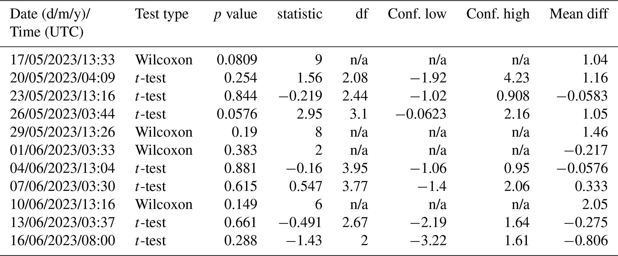
Differences in N₂O concentrations between the SML and the ULW were assessed separately for each sampling event. For each date and time, paired samples from SML and ULW collected simultaneously were compared. Prior to hypothesis testing, data distributions were evaluated for approximate normality. When the assumption of normality was met, paired t-tests were applied; otherwise, non-parametric Wilcoxon signed-rank tests were used. All tests were conducted as two-sided tests with a significance level of α= 0.05. Test statistics, p-values, and effect estimates were recorded for each sampling event (Table 1).

Table 1 Statistical test outcome for the comparison of SML and ULW sampling pairs. n/a: not applicable.

3 Results

3.1 Overview of general conditions and parameters in the mesocosm

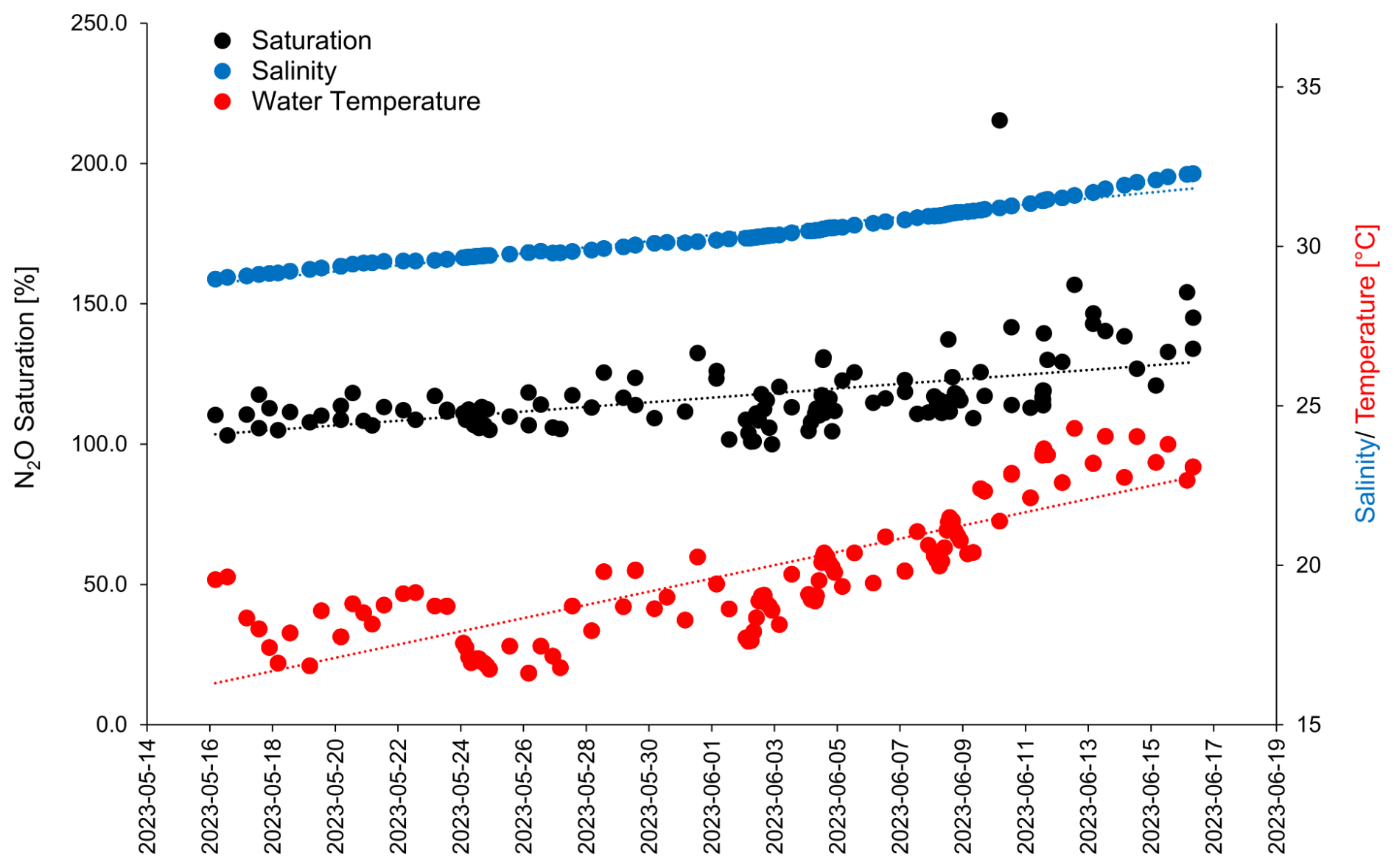
Chlorophyll a concentrations varied from 1.0 to 11.4 µg L⁻¹ and were affected by the nutrient additions which triggered a phytoplankton bloom (Bibi et al., 2025). Three phases of the bloom have been identified: (1) a pre-bloom phase from the start of the study until 26 May 2023, (2) a bloom phase from 27 May until 4 June 2023 and (3) the post-bloom phase from 5 June 2023 until the end of the study (Bibi et al., 2025). Haptophytes, specifically Emiliania huxleyi (Gephyrocapsa huxleyi), dominated the phytoplankton community, followed by diatoms, primarily Cylindrotheca closterium (Bibi et al., 2025). Enrichments of surfactants and dissolved organic carbon were observed after the bloom (data are shown in Bibi et al., 2025, Asmussen-Schäfer et al., 2026). Water temperatures were in the range of 16.6 and 20.3 °C until 2 June 2023 and then started to increase up to 24.3 °C on 12 June 2023. The salinity increased almost linearly during the study from 28.98 to 32.28 (Fig. 1).

Figure 1 Water temperature, salinity and N₂O saturation during the mesocosm study.

Nitrate (NO${}_{\mathrm{3}}^{-}$) and nitrite (NO${}_{\mathrm{2}}^{-}$) in the ULW and the SML, as well as nutrient additions to the mesocosm are shown in Fig. 2 (Bibi et al., 2025).

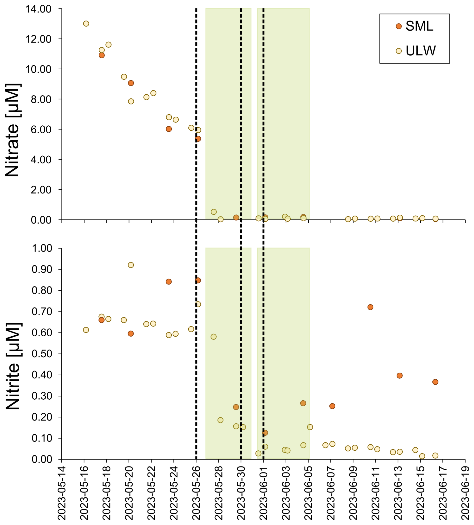
Figure 2 Dissolved nitrate (upper panel) and dissolved nitrite (lower panel) during the mesocosm study in the SML (filled red circles) and the ULW (filled yellowcircles). µM stands for 10⁻⁶ mol L⁻¹. The bloom is indicated by the green-shaded boxes. The timing of the nutrient additions is indicated by the three dashed lines.

NO${}_{\mathrm{3}}^{-}$ concentrations decreased steadily from the start of the study until the onset of the bloom on 27 May 2023. This was followed by a sharp drop of NO${}_{\mathrm{3}}^{-}$ concentrations which remained low (0.03–0.52 µmol L⁻¹) until the end of the study. Nitrite concentrations in both the ULW and SML dropped down as well when the bloom started on 27 May 2023. During the bloom and post-bloom phases the NO${}_{\mathrm{2}}^{-}$ concentrations remained low, whereas, the NO${}_{\mathrm{2}}^{-}$ concentrations in the SML increased again in the post-bloom phase to a maximum concentration of > 1 µmol L⁻¹ until 14 June 2023 (Bibi et al., 2025). With the exception of 20 May 2023, NO${}_{\mathrm{2}}^{-}$ was always enriched in the SML. Please note that from the 28. May onward the majority of the NO${}_{\mathrm{2}}^{-}$ concentrations in the SML and all of the NO${}_{\mathrm{2}}^{-}$ concentrations in the ULW were below the detection limit of 0.4 µmol L⁻¹.

3.2 N₂O concentrations, saturation and enrichment

N₂O concentrations in the SML and the ULW as well as chlorophyll a concentrations are shown in Fig. 3.

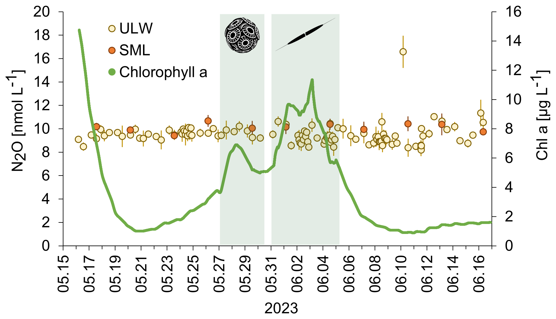
Figure 3 N₂O concentrations in the SML (filled red circles) and ULW (open circles) and chlorophyll a during the mesocosm study (green line). The green shaded boxes indicate the bloom. The inserted pictures show the haptophyte Emiliania huxleyi (Gephyrocapsa huxleyi) (left) and the diatom Cylindrotheca closterium (right). Early morning samples (30 min past sunrise): 20 and 26 May; 1, 7, and 13 June 2023. Afternoon samples (10 h past sunrise): 17, 23, and 29 May 2023; 4, 10, and 16 June 2023). There was no significant trend in N₂O concentrations over the time of the despite the two bloom periods and strong changes in the chlorophyll a concentration.

N₂O concentrations ranged from 9.4 to 10.7 nmol L⁻¹ and from 8.2 to 16.6 nmol L⁻¹ in the SML and the ULW, respectively. However, we excluded the single maximum concentration of 16.6 nmol L⁻¹, assuming it is an outlier. Mean N₂O concentrations in the mesocosm remained stable over the observation period (overall mean including SML and ULW ± SD: 9.62 ± 0.74 nmol L⁻¹). Despite of variations in other parameters, there were no significant temporal trends in N₂O concentration, this was supported by a generalized additive mixed model analysis (smooth term for time: edf = 1.0, F = 1.23, p = 0.27). This indicates the absence of both linear and non-linear long-term changes during the study period. A weak, non-significant diel pattern was observed (smooth term for time of day: edf = 1.31, p = 0.076), suggesting only minor diurnal variability. Overall, the model explained little of the observed variance (adjusted R²= 0.023), consistent with largely stable N₂O concentrations. The average N₂O concentration during the day was 9.4±0.7 nmol L⁻¹ and the average N₂O concentration during the night was 9.5±0.6 nmol L⁻¹. Diurnal cycles of N₂O concentrations in the ULW and light irradiance are shown in Fig. 4. Therefore, simple comparative statistics were deemed sufficient for further data analysis.

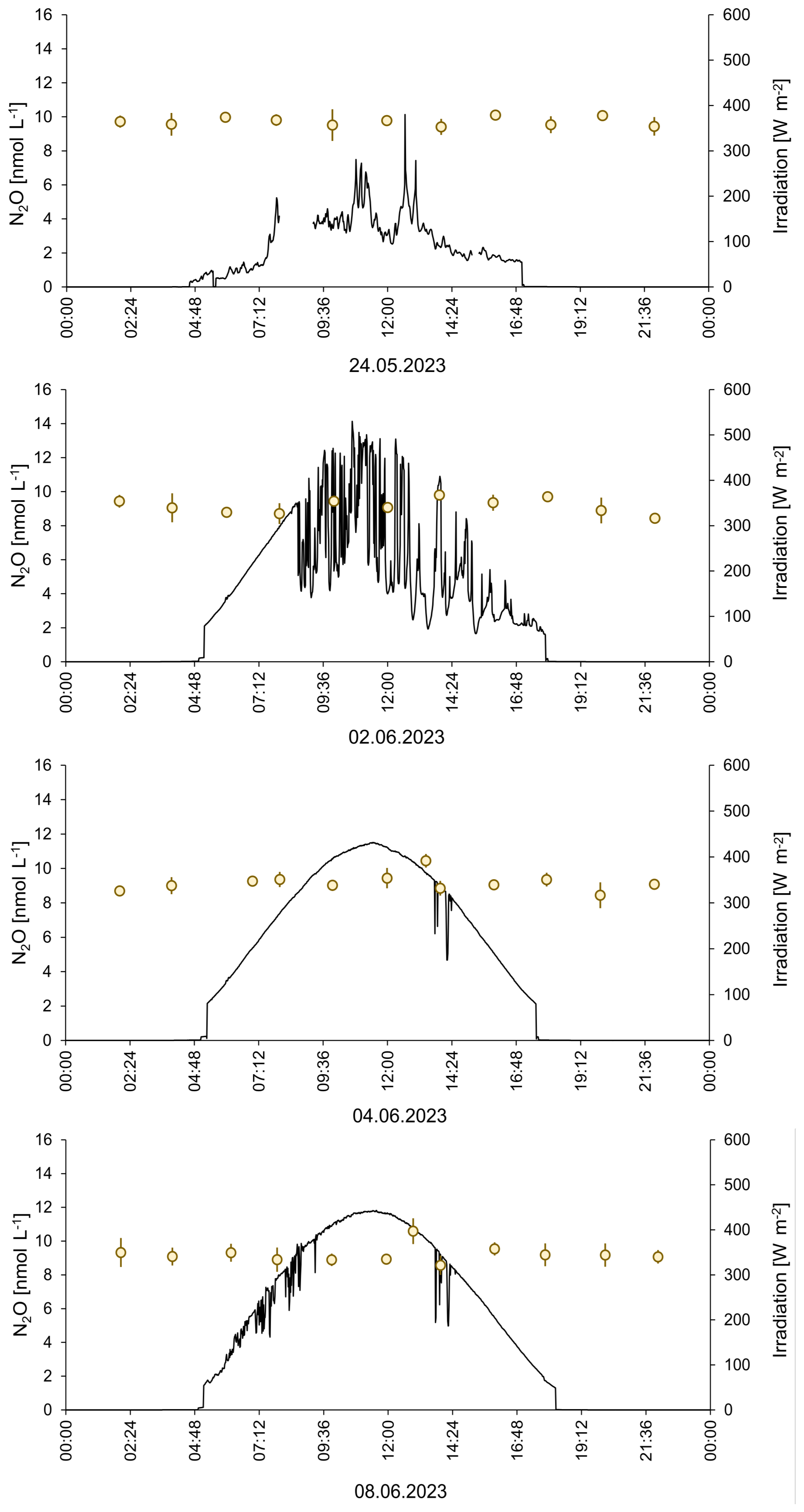
Figure 4 24 h measurements of N₂O concentrations on four days during the mesocosm study. The irradiance at a wavelength of 356 nm is shown.

Comparing the ULW and the SML N₂O concentrations, the overall averages (±standard deviation) for the samples taken in parallel for SML and UWL were 10.1±0.4 and 9.7±0.7 nmol L⁻¹, respectively. However, the difference between the average N₂O concentrations in the SML and the UWL was not significant according to the Student's t-test (two tailed, different variances, p>0.05). Between the N₂O concentrations of all single SML and ULW sampling pairs, no statistically significant differences were detected (all p > 0.05) (Table 1). While marginal differences were observed at individual time points (e.g. 26 and 17 May), these effects were not consistent in direction or magnitude across the study period (Table 1).

N₂O saturations in the SML and the ULW were in the range from 100 % to 157 % (215 % for the single maximum concentration from the ULW, Fig. 1). The enrichment factor of N₂O in the SML was in the range from 0.9 to 1.2 and the average enrichment factor (±standard deviation) was 1.1±0.1 indicating an overall enrichment. However, in a few cases EF${}_{{\mathrm{N}}_{\mathrm{2}}\mathrm{O}}$ < 1.0 was observed as well.

3.3 N₂O production and gas exchange

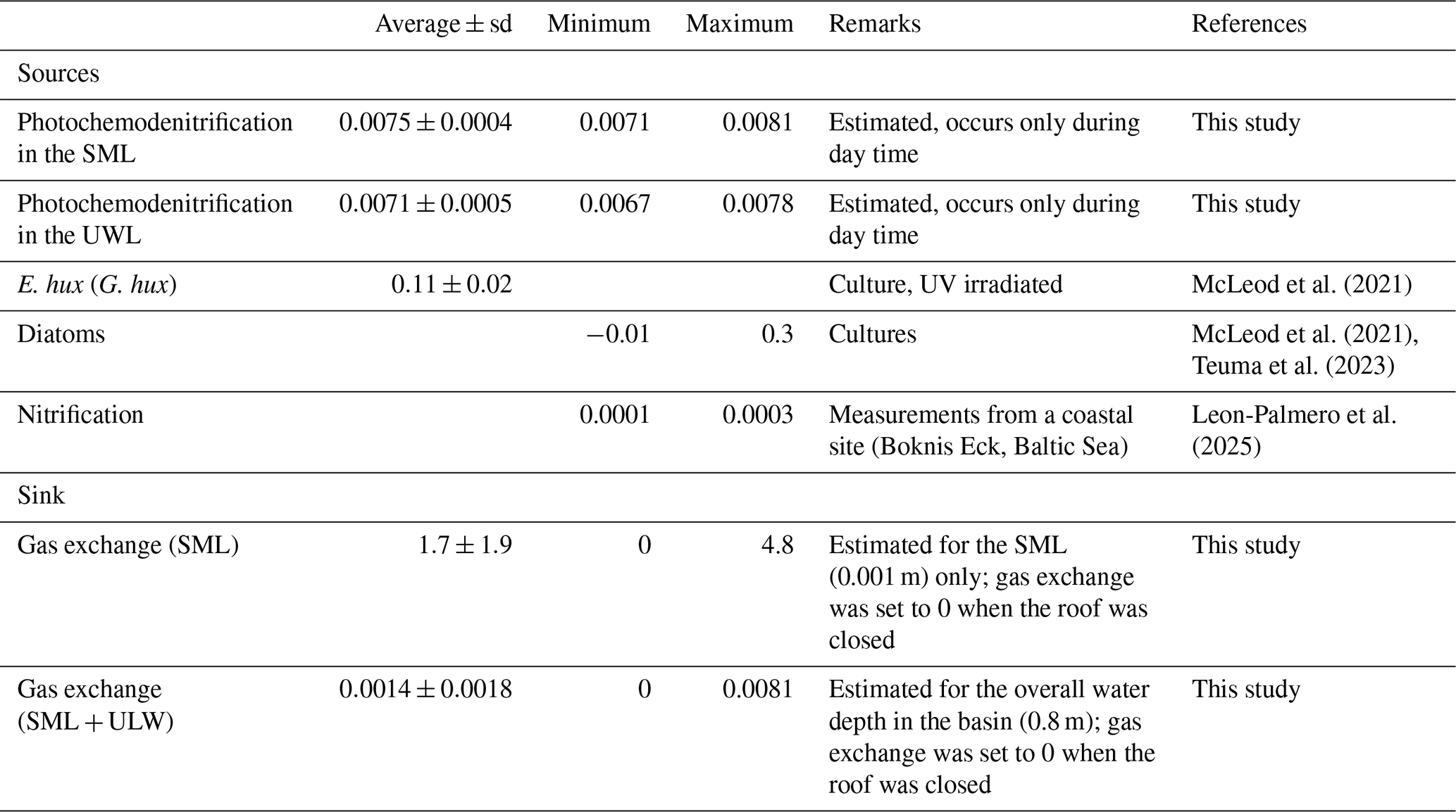
N₂O production rates via photochemodenitrification (PR_pcd) were calculated only for daylight samples and ranged from 0.0071 to 0.0081 nmol N₂O L⁻¹ h⁻¹ and from 0.0067 to 0.0078 nmol N₂O L⁻¹ h⁻¹ in the SML and ULW, respectively (Table 1). Although the mean PR_pcd in the SML (0.0075±0.0004 nmol L⁻¹ h⁻¹) was slightly higher compared to the PR_pcd in the ULW (0.0071±0.0005 nmol L⁻¹ h⁻¹), there was no statistically significant difference between the mean PR_pcd in the SLM and the ULW. The N₂O gas exchange (F_ase) was in the range from 0 to 4.8 nmol N₂O L⁻¹ h⁻¹ and 0 to 0.0081 nmol L⁻¹ h⁻¹ for the average thickness of the SML and the overall water depth (including N₂O concentrations from the SML and UWl, respectively (Table 1)).

Table 2 Potential N₂O sources and sinks (in nmol L⁻¹ h⁻¹). Sd stands for standard deviation.

4 Discussion

4.1 N₂O concentrations in the SML

Although lacking a statistic significance the overall average N₂O enrichment factor indicated a trend for a general enrichment of N₂O in the SML. This is further supported by the assumption that the measurements of N₂O in the SML are most probably underestimated because there is no proper SML sampling technique other than the glass plate (or the Gerrit screen) available to date, which prevents a loss of gases during the sampling procedure. A correction for those losses has been proven to be difficult because it depends on several, usually not quantified, factors and processes (see also Lange et al., 2025): (1) the dissolved gas saturation, because the exchange across the water/atmosphere interface on the glass plate is driven by the concentration difference between the atmosphere and the SML water. Thus, a high supersaturation will lead to an enhanced loss of gas compared to equilibrium saturations (and vice versa), (2) the amount of the surfactants in the SML. It is well-known that increasing amounts of surfactants can reduce the N₂O exchange across the water/atmosphere interface (Mesarchaki et al., 2015), (3) altered shear conditions compared to the ambient sea surface: When the glass plate is moved out of the water, the film of SML water on the glass plate is subjected to altered shear and airflow orientation relative to the ambient wind field. which can lead to an enhanced release of gas across the water/atmosphere interface, and (4) the physical properties of N₂O, especially solubility and diffusivity, that are driven by temperature and salinity. Overall, there seems to be no universal loss factor considering all in-situ variables (e.g. the amount of the prevailing surfactants) and any estimate of the loss factor, e.g. in laboratory experiments, is thus challenging because it depends mainly on in-situ field conditions which are difficult to mimic in laboratory experiments. Comparative studies for other dissolved gases (e.g. dimethyl sulfide) indicate that different sampling approaches can yield systematically different enrichment factors, highlighting the sensitivity of gas-phase measurements to sampling-induced artefacts (Saint-Macary et al., 2023; Yang et al., 2001). Since no estimates of the N₂O loss during glass plate sampling are available to our knowledge, the N₂O concentrations in the SML presented here were not corrected.

Based on the fact that we measured supersaturations of N₂O in the SML we conclude that there must have been a significant enrichment of N₂O in the SML during the course of the mesocosm study. This is in line with the suggestion of Leon-Palmero et al. (2025) of a UV light-driven photochemical production of N₂O (i.e. photochemodenitrification) which should be more enhanced in the SML because the SML is directly exposed to the sunlight. The fact that nitrite concentrations in the SML were higher than in the ULW does not counteract photochemodenitrification, because the overall nitrite concentrations are dominated by (micro)biological processes in the SML.

4.2 N₂O saturations

N₂O saturations in both the SML and the ULW were ≥ 100 % during the course of the study. The general supersaturation (= excess) of dissolved N₂O was obviously resulting from a net in-situ production of N₂O in the water. Therefore, the water in the mesocosm basin was a source for atmospheric N₂O during the course of the study. The apparent increasing trend of the N₂O saturations is resulting from the increasing temporal trends of the water temperature and the salinity (Fig. 1) which resulted in a reduced N₂O solubility and therefore a decreasing trend in the N₂O equilibrium concentrations while the measured N₂O concentrations in the SML and the ULW showed no temporal trend (Fig. 3). Additionally, a decrease in air sea gas exchange towards the end of the study may have also contributed to increasing N₂O saturations. However, due to technical issues and therefore missing wind speed data for this time period, we were not able to test this assumption.

4.3 Sources and sink of N₂O

The accumulation of N₂O concentrations in the SML and the ULW (as reflected by the persistent supersaturations in both layers, see section above) resulted from its in-situ production. Potential N₂O sources are photochemodenitrification, release from phytoplankton and microbial nitrification. The estimated photochemical production rates (PR_pcd) from both the SML and the ULW (see Table 2) are at the lower end of the so far observed N₂O production rates from photochemodenitrification in coastal and fresh water systems (Leon-Palmero et al., 2025). However, it has to be noted that the NO${}_{\mathrm{2}}^{-}$ concentrations were below the detection limit during the last half of the study for the majority of measurements. Therefore, PR_pcd estimates may not be fully reliable for this particular time hampering the ability to identify diel variations in photochemodenitrification rates. N₂O production by marine phytoplankton can range from −0.06 to 0.99 nmol L⁻¹ h⁻¹ (McLeod et al., 2021). The specific N₂O production rate of E. hux (G. hux) as determined in a culture study under UV irradiation was 0.11±0.02 nmol L⁻¹ h⁻¹ (McLeod et al., 2021). While there is no rate available for C. closterium a culture study with other diatom species (incl. Thalassiosira weissflogii, Thalassiosira pseudonana, Skeletonema marinoi and  Cyclotella cryptica) revealed N₂O production rates from −0.01 to 0.3 nmol N₂O L⁻¹ h⁻¹ (McLeod et al., 2021; Teuma et al., 2023) which are in the same range as the rates reported for E. hux (G. hux). N₂O production rates via nitrification in oxic waters, such as found in the mesocosm study with dissolved oxygen concentrations > 240 µmol L⁻¹ (Rauch et al., 2026) are usually low: For example, N₂O production rates from ammonia oxidation (i.e. the first step of microbial nitrification) measured at the Bokins Eck coastal time-series site located in Eckernförde Bay (SW Baltic Sea) were found to range from 0.0001 to 0.0003 nmol N₂O L⁻¹ h⁻¹ (Leon-Palmero et al., 2025). This is in line with the fact that prevailing high oxygen concentrations do not favour N₂O production by nitrification (see e.g. Fig. 6 in Santoro et al., 2021). On the other hand, studies suggest that microenvironments around particles, including dead diatom aggregations, may provide oxygen depleted reaction space in which denitrification and N₂O production may occur despite high dissolved oxygen concentrations within the surrounding water column (Ciccarese et al., 2023). However, the scale of N₂O production around these particles is yet unknown. Therefore, the in-situ production of N₂O during the mesocosm study was most likely resulting from photochemodenitrification and by the release from phytoplankton with only a minor contribution from nitrification.

The time-series of N₂O concentrations in both the SML and ULW showed no temporal trends which indicate that the N₂O concentrations were not affected by enhanced N₂O production during the bloom, especially from the two bloom-dominating species E. hux (G. hux) and C. closterium. On the one hand, this seems to contrast the findings from various culture experiments which showed that haptophytes and diatoms have the potential to produce and release N₂O (McLeod et al., 2021; Teuma et al., 2023). On the other hand, naturally as well as anthropogenically triggered phytoplankton blooms in the ocean did not result in enhanced N₂O concentrations during the blooms (Farías et al., 2015; Law and Ling, 2001; Walter et al., 2005). The obvious negligible effect of the phytoplankton bloom on N₂O concentrations during the mesocosm study (and other oceanic areas) does not exclude a N₂O release from phytoplankton per-se, but suggests that N₂O release was low and that the N₂O production rates resulting from culture studies may not be representative for natural ecosystems.

The high-resolution 24 h-sampling for N₂O in the ULW took place during the pre-bloom phase (24 May 2023), during the bloom (2 June and 4 June 2023) and during the post-bloom phase (8 June 2023). Neither the different phases of the bloom nor the solar irradiation affected the N₂O concentrations (Fig. 4). This finding, in combination with the missing trend over the entire period of the study, indicates that the N₂O concentrations in both the SML and UWL were in a steady state, where the in-situ sources were counterbalanced by the release of N₂O to the overlying atmosphere: Approximate estimates of the average N₂O gas exchange in this study range from 0 to 6.5 nmol N₂O L⁻¹ h⁻¹ (Table 2) and are, therefore, high enough to counteract the N₂O production. The comparatively high N₂O gas exchange rates estimated in this study reflect the specific physical conditions of the mesocosm setup rather than open-ocean air-sea exchange. The parameterization of Liss and Merlivat (1986), derived primarily from wind–water tunnel experiments, was therefore considered most appropriate, as it accounts for gas transfer under limited fetch and small-scale wind-wave conditions comparable to those in the mesocosms. In contrast, commonly used open-ocean parameterizations (e.g. Wanninkhof, 2014) are based on fully developed wave fields and substantially larger fetches, which are not representative of the experimental conditions. Consequently, applying such formulations would likely underestimate gas exchange in the present setup. Please note, however, that the approach of (Liss and Merlivat, 1986) does not account for the effect of surfactants. So, F_ase is most probably overestimated. However, given the high uncertainties associated with the estimates of the sources and sink of N₂O listed in Table 2, we can assume that the N₂O sources were balanced by the N₂O gas exchange flux. The photochemical production as well as the release by phytoplankton occurs during day time only because they are light-dependent. Because the roof of the mesocosm facility was closed during the night, the wind-driven N₂O gas exchange took place only during day time as well. This might explain the absence of the diurnal cycles since both the sources and the sink of N₂O were only active during the day but not during the night. This could have led to the establishment of a steady state during the day time which persisted during night time because sources and the sink were not active during the night.

5 Conclusions

N₂O was measured during a mesocosm study in the ULW and, for the first time, in the SML. N₂O concentrations were slightly enriched in the SML, although the difference of the mean N₂O concentrations between the SML and ULW was statistically not significant. However, the enrichment of N₂O in the SML was most probably underestimated due to the loss of N₂O during sampling with the glass plate method. Consequently, a significant enrichment of N₂O in the SML may result in an enhanced N₂O release to the atmosphere. Therefore, estimates of N₂O emissions which do not account for the N₂O enrichment in the SML most probably underestimate the N₂O flux to the atmosphere. N₂O was supersaturated in the SML and ULW during the course the mesocosm study which indicated an in-situ production of N₂O. N₂O in-situ production was most probably dominated by photochemodenitrification in combination with the release from phytoplankton. Microbial production of N₂O via nitrification was assumed to be of minor importance because of the prevailing high oxygen concentrations which do not favour N₂O production via nitrification. The N₂O in-situ sources were obviously balanced by the release of N₂O to the overlying atmosphere and thus the system was in a steady state. Therefore, N₂O concentrations in both the SML and the UWL were remarkably constant over time showing no diurnal cycles and no enhanced N₂O concentrations during the phytoplankton bloom. Our results are thus in line with the results from field studies which showed that phytoplankton blooms in the ocean do not result in temporarily enhanced N₂O concentrations in the ocean surface layer.

The results presented here indicate that the role of the SML for N₂O cycling in the surface ocean has been overlooked so far. It seems to be more important than previously thought. Future studies should, therefore, identify and quantify the N₂O sources and sinks in the SML. Moreover, our results highlight the need for continued methodological refinement to better constrain sampling-induced losses of dissolved trace gases in the SML, which remain a key uncertainty for reliable N₂O emission estimates.