Seasonal to long-term variability of natural and anthropogenic carbon concentrations and transports in the subpolar North Atlantic Ocean

The Atlantic Meridional Overturning Circulation (AMOC) is integral to the climate system, transporting heat and anthropogenic carbon across the North Atlantic (NA) from subtropical to subpolar latitudes. This physical mechanism promotes the uptake and sequestration of atmospheric CO₂ through surface cooling as warm water advances northward and consequently sinks through deep winter convection. Using ship-based observations, ocean reanalyses, neural networks, and a back-calculation approach, we present a 30-year monthly time series of contemporary carbon (natural, C_nat and anthropogenic, C_ant) concentrations and transports at the A25-OVIDE hydrographic section in the subpolar NA Ocean, and assess their variability from seasonal to long-term scales. We divided the section into essential layers, including the upper branch of the AMOC (uMOC) and the mixed layer (ML). Our findings indicate that the full-section-averaged C_nat concentration shows no significant trend over the 30-year period. In contrast, the full-section-averaged C_ant concentration increased by more than one third over the 30-year period, attributed to the anthropogenic increase in atmospheric CO₂. Seasonal and interannual variability is more pronounced in the uMOC and in the ML, where deep convection and biological activity impact their concentration, than in the deeper ocean. The seasonal deepening of the ML in winter contributes two thirds and one half of its ML concentration for C_nat and C_ant, respectively, the rest being attributed to biology and solubility. The C_ant and C_nat transports are predominantly determined by the variability of volume transport, except for the decadal trend in C_ant transport which is primarily influenced by changes in C_ant concentration. The variability in tracer transport is the largest in the uMOC, which exhibits a seasonal peak-to-peak amplitude of approximately 25 % of the annual mean tracer transport. These results offer new insights to refine model representations and improve our understanding of the subpolar NA carbon dynamics.

1 Introduction

The atmospheric CO₂ concentration has surged by 50 % since the onset of the industrial revolution in the 1750s, surpassing 420 ppm in 2023 (Keeling et al., 2005). In response to this rapid increase, the ocean acts as a vital carbon sink, absorbing 2.9 ± 0.4 PgC yr⁻¹ from the atmosphere and therefore compensating for approximately a quarter of total annual CO₂ emissions (Friedlingstein et al., 2025). This oceanic uptake is facilitated by the massive carbon storage capacity of the ocean –its dissolved inorganic carbon (DIC) reservoir is approximately 50 times larger than the atmospheric reservoir (Friedlingstein et al., 2025). The oceanic DIC pool can be divided into its natural (C_nat) and anthropogenic (C_ant) fractions, such that DIC = C_nat + C_ant. C_nat includes preformed DIC as well as DIC resulting from the biological and carbonate pumps.

The ocean's ability to absorb atmospheric CO₂ and redistribute DIC within the water column is governed by the interplay of physical and biological processes – namely physical and biological carbon pumps (PCP and BCP), respectively – operating within or close to the ocean mixed layer (ML). The oceanic mixed layer (ML) corresponds to the near-surface layer of the ocean where turbulent processes, primarily induced by wind forcing, buoyancy fluxes, and wave breaking, maintain quasi-homogeneous temperature (T), salinity (S) and dissolved oxygen (O₂) profiles. It represents the portion of the ocean directly interacting with the atmosphere, where weak vertical gradients may still persist. The depth of the ML is generally defined from a threshold criterion based on potential density or temperature relative to surface values. Within the ML, the PCP operates through CO₂ solubility – enhanced in colder waters – and vertical mixing. Meanwhile, the BCP encompasses the photosynthetic fixation of DIC by phytoplankton, followed by sinking and remineralization of organic matter at depth (Dall'Olmo et al., 2016; Diaz et al., 2021; Lacour et al., 2019). By modulating carbon uptake and redistribution, the ML thus plays a pivotal role in climate regulation (Sallée et al., 2021).

The ocean's capacity to absorb and store CO₂ is not spatially homogeneous. The North Atlantic (NA), characterized by the deepest ML in the world, complex physical dynamics, and strong biological activity, plays a significant role in the uptake and storage of global CO₂ uptake and storage (Dall'Olmo et al., 2016; Resplandy et al., 2018; Pérez et al., 2010, 2013, 2024). Despite covering only 15 % of the global surface ocean, the NA accounts for approximately 25 % of contemporary global CO₂ ocean uptake and a quarter of the global ocean C_ant inventory (DeVries, 2014; Friedlingstein et al., 2019; Gruber et al., 2019; Khatiwala et al., 2013), which is the highest per unit area of the global ocean (Gruber et al., 2023; Sabine et al., 2004). The latter is partly related to the Atlantic Meridional Overturning Circulation (AMOC). The upper limb of the AMOC drives the poleward transport of C_ant from the subtropics to the subpolar NA (Brown et al., 2021; Pérez et al., 2013; Zunino et al., 2015, 2014), a regional convergence zone where the deepest penetration of C_ant occurs (Sabine et al., 2004; Mikaloff Fletcher et al., 2006). Previous studies have highlighted the sensitivity of C_ant transport to the strength of the AMOC (Boers, 2021; Caesar et al., 2021, 2018; Jackson et al., 2022; Thornalley et al., 2018), with implications for carbon sequestration and air-sea fluxes (Pérez et al., 2013; Zunino et al., 2015; Brown et al., 2021) (Liu et al., 2023; Pérez et al., 2013).

Discrepancies persist between observational estimates and model simulations, particularly with regard to ocean C_ant and C_nat transports (Racapé et al., 2018; Tjiputra et al., 2010; Mikaloff Fletcher et al., 2006), and the sea surface partial pressure of CO₂ (pCO₂) driving air-sea fluxes (Rodgers et al., 2023). Although individual cruises provide indispensable reference estimates, they do not fully capture the temporal variability in the transport and concentration of C_ant and C_nat (Zunino et al., 2015, 2014; McCarthy et al., 2015; Mercier et al., 2024). The magnitude, variability and factors that govern the contribution of ocean circulation to regional storage of C_ant or C_nat, and consequently the resilience of the ocean carbon sink to global changes, thus remain largely unexplored (Hauck et al., 2020; Henson et al., 2022).

In particular for the SubPolar North Altantic (SPNA), most studies have focused mainly on decadal changes, with biennial cruises measuring C_nat and C_ant transports (Zunino et al., 2014, 2015; Fontela et al., 2019), or on high-temporal-resolution volume transports (McCarthy et al., 2015; Caesar et al., 2021; Fu et al., 2023; Tooth et al., 2023; Mercier et al., 2024), but there is still a dearth of high-temporal-resolution tracer transport data. This study addresses this research gap by presenting the first 30-year observation-based monthly time series of surface-to-bottom C_nat and C_ant transport across the A25-OVIDE Greenland to Portugal section in the northern North Atlantic (Fig. 1) between 1993 and 2022. By combining ship-based data, ocean reanalyses, neural networks (NN), and a back-calculation (BC) approach for ocean C_ant estimation, this research aims to improve our understanding of seasonal to long-term variability in C_nat and C_ant concentrations (hereinafter marked as [C_nat] and [C_ant]) and transports. It will contribute to improve the predictions of carbon uptake and storage in the NA by providing a novel and comprehensive assessment of the regional surface-to-bottom seasonal cycles and long-term trends. We decompose the net transport of C_nat and C_ant into vertical layers to differentiate various signals: we split the water column into the upper and lower limbs of the AMOC (uMOC and lMOC, respectively) and also distinguish between the ML and what lies beneath it (bML).

2 Data and methods

This study is based on the Greenland-to-Portugal OVIDE section, known as A25 by GO-SHIP (Sloyan et al., 2019). We used two types of data: (1) hydrographic data (T, S, [O₂], nutrients, total alkalinity [A_T], pH, velocities) from the 1997 FOUREX cruise and from the 2002–2018 A25 OVIDE biennial repeats (Sect. 2.1), referred to as reference dataset; and (2) ocean reanalysis data (velocities, T, S monthly gridded fields) at the A25-OVIDE section (Sect. 2.2). We applied NN algorithms to the reanalysis property data to generate monthly gridded fields of [O₂], nutrients, [A_T] and [DIC] (Sect. 2.4). Using hydro- and NN-based reanalysis property datasets, we used a back-calculation approach (Sect. 2.3) to calculate [C_ant], [C_nat] being the difference between [DIC] and [C_ant]. The so-derived [C_ant] and [C_nat] fields were then combined with the corresponding velocity fields to compute the time series of cross-A25 section C_ant and C_nat transports (Sect. 2.5). C_ant and C_nat transports were divided into different vertical regions (Sect. 2.6) to assess their seasonal to interannual and long-term variability (Sect. 2.7). Finally, we evaluated the performance of our ocean reanalysis-NN-BC method (hereinafter referred to as OR-NN-BC method) and its error in Sect. 2.8.

2.1 GO-SHIP A25 OVIDE hydrographic section

The Portugal-to-Greenland GO-SHIP A25 OVIDE hydrographic section (Fig. 1), referred to here as A25, has been repeated biannually in summer since 2002 (Mercier et al., 2024; Sloyan et al., 2019). This study uses data from nine A25 cruise repeats that span 2002–2018. To extend the reference dataset further back in time, data from the FOUREX 1997 cruise (Álvarez et al., 2003; Lherminier et al., 2007), which differs slightly from the A25 positions, have also been included. The T and S of the CTD sensors are collocated with nutrients (nitrate, phosphate, and silicate), [A_T], pH and [O₂] from bottle samples. BGC data consistency was ensured by applying the GLODAP recommended adjustments to the measured values of [O₂], nitrate, phosphate, silicate, pH and [A_T] (see “Recommended adjustment values” at https://glodapv2.geomar.de, last access: 17 October 2023) (Olsen et al., 2019). We used these data to compute C_nat and C_ant (Sect. 2.3), which are used here in conjunction with absolute velocities to compute property transports (Sect. 2.5) (Daniault et al., 2016; Zunino et al., 2017, 2015, 2014; Pérez et al., 2013; Fontela et al., 2019; Lherminier et al., 2007, 2010; Gourcuff et al., 2011; Mercier et al., 2024). Geostrophic velocities were derived by integrating geostrophic shears, calculated from T and S data obtained at hydrographic stations, using as reference simultaneous velocity measurements from a Ship-mounted Acoustic Doppler Current Profiler (S-ADCP). Ekman transport, estimated from NCEP data, was incorporated into the surface layer (0–30 m). An inverse model was applied to compute velocity corrections for each pair of hydrographic stations to ensure volume conservation (see Lherminier et al., 2007, 2010; Gourcuff et al., 2011; Mercier et al., 2024, 2015; Daniault et al., 2016; Zunino et al., 2014). The A25 velocities v used here are normal to the section and correspond to geostrophic velocities plus Ekman velocities (Lux et al., 2001; Lherminier et al., 2007).

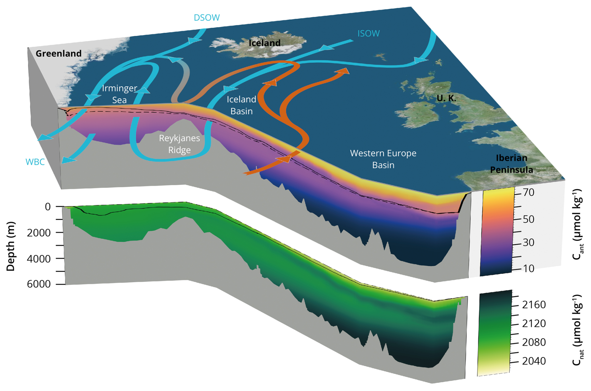
Figure 1 North Atlantic subpolar region and the GO-SHIP A25 OVIDE hydrographic section (called A25 here). The arrows represent the main currents at the A25 section: the NAC, the Western Boundary Current (WBC) including the East Greenland Current (EGC), the Iceland–Scotland Overflow Water (ISOW) and the Denmark Strait Overflow Water (DSOW). Natural carbon [C_nat] and anthropogenic carbon [C_ant] calculated from the T, S fields from the GLOSEA5 reanalysis (see Sect. 2.4) are displayed at A25 for the last year of the study (2022) in the bottom and top panels, respectively (see Sect. 2). Winter and summer mean mixed layer depths from GLOSEA5 are shown as solid and dashed lines respectively for [C_nat]. The isopycnal σ_MOC, separating the upper and lower limbs of the AMOC, from GLOSEA5 is shown on [C_ant] for April (32.24 kg m⁻³ for a density anomaly referenced at 1000 db) and October (32.13 kg m⁻³), which are the months with the strongest and weakest seasonal transports in the upper branch of the uMOC respectively. Bathymetry is from GEBCO.

2.2 Ocean products

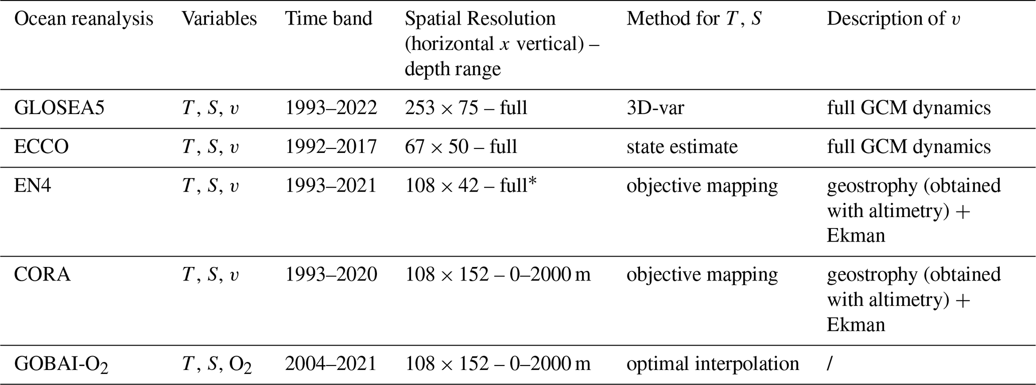
The ocean reanalysis datasets used (Table 1) are GLOSEA5 (Scaife et al., 2014; MacLachlan et al., 2015), ECCO (Fenty and Wang, 2020), EN4 (Good et al., 2013) and CORA (Szekely et al., 2019). Ocean reanalyses are data-driven products with varying levels of complexity, and each individual product has its own strengths and limitations. Using the mean concentration across products helps mitigate product-specific biases and errors, while the spread among them provides an estimate of the associated uncertainty. All reanalyses provide gridded T and S at monthly resolution. The velocity fields (v) of CORA and EN4 are geostrophic velocities derived from T, S, surface altimetry, while the Ekman velocities are derived from NCEP (Mercier et al., 2024) (Table 1). Velocities for GLOSEA5 and ECCO are full general circulation model (GCM) dynamics (Mercier et al., 2024). EN4 and CORA were interpolated to the positions of the A25 section. For ECCO and GLOSEA5 GCM, the nearest native grid points to the A25 section were used. The reader is referred to Mercier et al. (2024) for a detailed discussion of seasonal to long-term volume transport variability at A25 from GLOSEA5, ECCO, EN4, and CORA. To complement the ocean reanalysis datasets, we also considered the use of the GOBAI-O₂ gridded product (Sharp et al., 2023) (version 1.1). GOBAI-O₂ provides O₂ monthly fields computed by applying NN to gridded monthly T and S fields derived from Argo (Roemmich and Gilson, 2009). The original GOBAI-O₂ data (1° ×1° resolution on 58 depth levels) were interpolated to the positions of the A25 section (Table 1). The use of GOBAI-O₂ might introduce additional depth-dependent biases in O₂ associated to Argo-O₂ sensors (Bushinsky et al., 2025). Our error estimation method, based on the comparison to the A25 ground truth (see Sect. 2.8), ensures that any potential bias from the use of GOBAI-O₂ is reflected in the reported uncertainties.

Table 1 Ocean products, with their time band and their depth range at the A25 section. All ocean products include monthly average values of temperature (T) and salinity (S). Ocean reanalyses also include velocity data and GOBAI-O₂, dissolved oxygen (O₂). ^* Note that for EN4, the T and S fields are provided for the entire water column, but the velocity data are restricted to the depth range 0–2000 m (see Mercier et al., 2024) (Table 2). The reader is referred to Mercier et al. (2024) for more details on the ocean reanalysis data.

2.3 Anthropogenic and natural carbon estimates

To determine the C_ant fraction from [DIC], we used the carbon-based BC $\mathit{\phi }{C}_{\mathrm{T}}^{\mathrm{0}}$ approach (Pérez et al., 2008; Vázquez-Rodríguez et al., 2009). This BC approach has been broadly applied to study the inventory of C_ant, its storage rates, its variability (Pérez et al., 2008; Vázquez-Rodríguez et al., 2009; Pérez et al., 2013; Fröb et al., 2018; Asselot et al., 2024) and the influence of C_ant on ocean acidification (Pérez et al., 2018). The input variables for this approach include date, geographical location, T, S, O₂, macronutrients (NO${}_{\mathrm{3}}^{-}$, PO${}_{\mathrm{4}}^{\mathrm{3}-}$ and Si(OH)₄), [A_T] and [DIC]. To estimate the natural carbon concentration [C_nat], [C_ant] (Sect. 2.3) is subtracted from [DIC] ([C_nat] = [DIC] − [C_ant]). For reference data, T, S, [O₂], macronutrients, [A_T], and pH are measured at A25 bottles. [DIC] is derived from [A_T] and pH from the in situ bottle measurements using the PyCO2SYS toolbox (Humphreys et al., 2022) (version 1.8). This toolbox also provides the Revelle factor shown in this study. NNs are used to derive the necessary parameters for ocean reanalysis to obtain [C_ant] (Sect. 2.4).

2.4 Choice and application of neural networks

Two different NNs were sequentially applied to ocean reanalysis data to estimate [DIC] and the evaluation of the error is detailed in Sect. 2.8. Each NN has limitations, and the use of two different NNs was intended to build on the strengths of each NN. First, we applied ESPER NN (Carter et al., 2021, Eq. 8) to the T and S fields of the reanalysis (as well as date and position, i.e., longitude, latitude, and depth) as input to determine [O₂] and macronutrients. Second, we calculate [DIC] and [A_T] using CANYON-B NN – CONTENT (Bittig et al., 2018). CANYON-B uses the same input data as ESPER NN plus [O₂] (O₂ derived from ESPER_NN). The choice of ESPER NN and CANYON-B-CONTENT for the estimation of oxygen and macronutrients and carbon variables, respectively, is based on the performance of the corresponding NNs for each variable (i.e. lowest final error) (Asselot et al., 2024). Using ESPER alone to calculate [DIC], we found that [DIC] values diverged from cruise-based estimates after 2010, whereas between CANYON-B-CONTENT and observations there was a better agreement (Fig. S1 in the Supplement). Instead of a time-dependent prediction of [DIC] as in CANYON-B (Bittig et al., 2018), [DIC] is given for a reference year (2002) in ESPER. Within this NN, the anthropogenic component of DIC (C_ant) is calculated as an exponential increase (see Carter et al., 2021, their Eq. 1), assuming that C_ant is in a transient steady state (Tanhua et al., 2007) (that is, exponential increases in atmospheric anthropogenic CO₂ should result in the concentration of marine C_ant that increases at rates proportional to the concentration of atmospheric anthropogenic CO₂). The use of ESPER NN to estimate [O₂] and macronutrients and CANYON-B-CONTENT to estimate [DIC] and [A_T] is therefore a reliable compromise for applying NN to T and S fields in the subpolar gyre (Fig. S1). In the particular case of the GOBAI-O₂ dataset (Table 1), we applied ESPER NN only to retrieve macronutrients, then CANYON-B-CONTENT to retrieve [DIC] and [A_T] (Asselot et al., 2024). It is important to note that the A25 2002–2014 data used in this study to obtain the reference estimates are among the source data used for the training phase of both NNs: GLODAPv2.2019 (Olsen et al., 2019; Carter et al., 2021) and GLODAPv2 (Bittig et al., 2018; Olsen et al., 2016). However, the reference estimates from the A25 data for 2016 and 2018 can be considered entirely independent of those obtained using the OR-NN-BC method.

2.5 Transport calculation

2.5.1 Definition

Transport refers to the cross-section volume transport at A25. Net transport at a given time t (both for the A25 hydrographic data and ocean reanalyses), T(t) (Eq. 1) is expressed in Sverdrup (10⁶ m³ s⁻¹), with the integration performed over z from surface (z₁=0) to bottom ($z_{\mathrm{2}}=z_{max}\left(x\right)$) and over x from Portugal to Greenland along the A25 line.

$$\begin{array}{}\text{(1)}& T\left(t\right)={\displaystyle \frac{\mathrm{1}}{{\mathrm{10}}^{\mathrm{6}}}}\underset{x}{\int }\underset{z_{\mathrm{1}}}{\overset{z_{\mathrm{2}}}{\int }}v(x,z,t)\mathrm{d}x\mathrm{d}z\end{array}$$

The velocity field $v(x,z,t)$ (Table 1) refers to the absolute velocities normal to the section. The concentration $c(x,z,t)$ of [C_nat] or [C_ant] (expressed in  µmol kg⁻¹) and the velocities $v(x,z,t)$ obtained from the A25 cruise and ocean reanalysis are used to calculate the net transport of property T_p(t), in kmol s⁻¹ or PgC yr⁻¹. T_p(t) is calculated by integrating the section and multiplying the property by the flow velocity and density (Eq. 2). The transport of C_nat ($T_{C_{\mathrm{nat}}}$) and the transport of C_ant ($T_{C_{\mathrm{ant}}}$) are thus determined as:

$$\begin{array}{}\text{(2)}& T_{\mathrm{p}}\left(t\right)={\displaystyle \frac{\mathrm{1}}{{\mathrm{10}}^{\mathrm{9}}}}\underset{x}{\int }\underset{z_{\mathrm{1}}}{\overset{z_{\mathrm{2}}}{\int }}\mathit{\rho }(x,z,t)\cdot c(x,z,t)\cdot v(x,z,t)\mathrm{d}x\mathrm{d}z\end{array}$$

For the different transport estimations, volume and tracer transports (Eqs. 1, 2), positive (negative) transport means northward (southward) transport. The integration limits in z may vary according to the layer of the water depth column considered (see Sect. 2.6 for details on the vertical layer separations).

2.5.2 Diapycnal and isopycnal decomposition

Following previous studies on heat (Mercier et al., 2015), fresh water (McDonagh et al., 2015) or property transport (Álvarez et al., 2003; Zunino et al., 2014), we decomposed net property transport into a diapycnal and isopycnal term (Eq. 3). The diapycnal term refers to the transport of property associated with the overturning circulation, which accounts for the conversion of light to dense water masses north of the section (Grist et al., 2014). The isopycnal term refers to the gyre circulation and is the area integration of the covariance of the volume transport and property anomalies at each longitude and density level along the A25 section. This term is called horizontal circulation when decomposition is performed in pressure coordinates (Böning and Herrmann, 1994). The net' transport is the net transport of property through the section related to the net northward volume transport of approximately 1 Sv associated with the Arctic mass balance (Lherminier et al., 2007). We decompose the property and velocity as $c(x,\mathit{\sigma },t)=<c{>}_x(\mathit{\sigma },t)+c^{\prime \prime }(x,\mathit{\sigma },t)$ (for C_ant and C_nat), $v(x,\mathit{\sigma },t)=<v{>}_{x,\mathit{\sigma }}\left(t\right)+<v{>}_x(\mathit{\sigma },t)+v^{\prime \prime \prime }(x,\mathit{\sigma },t)$ , where given a quantity a and some spatial direction b we define $<a{>}_b=\frac{{\int }_{b}a\left(b\right)\mathrm{d}b}{{\int }_b\mathrm{d}b}$. As explained in Zunino et al. (2015), Eq. (2) can be rewritten as:

$$\begin{array}{}\text{(3)}& T_{\mathrm{p}}\left(t\right)=T_{\mathrm{p}}^{{\mathrm{net}}^{\prime }}\left(t\right)+T_{\mathrm{p}}^{\mathrm{diap}}\left(t\right)+T_{\mathrm{p}}^{\mathrm{isop}}\left(t\right)\end{array}$$

where $T_{\mathrm{p}}^{{\mathrm{net}}^{\prime }}\left(t\right)=<v{>}_{x,\mathit{\sigma }}\left(t\right)\cdot {\int }_x{\int }_{\mathit{\sigma }}<\mathit{\rho }\cdot c{>}_x(\mathit{\sigma },t)\mathrm{d}x\mathrm{d}\mathit{\sigma }$, $T_{\mathrm{p}}^{\mathrm{diap}}\left(t\right)={\int }_x{\int }_{\mathit{\sigma }}<v{>}_x(\mathit{\sigma },t)\cdot <\mathit{\rho }\cdot c{>}_x(\mathit{\sigma },t)\mathrm{d}x\mathrm{d}\mathit{\sigma }$ and $T_{\mathrm{p}}^{\mathrm{isop}}\left(t\right)={\int }_x{\int }_{\mathit{\sigma }}{v}^{\prime \prime \prime }(x,\mathit{\sigma },t)\cdot \mathit{\rho }\cdot c^{\prime \prime }(x,\mathit{\sigma },t)\mathrm{d}x\mathrm{d}\mathit{\sigma }$.

2.6 Region separation

2.6.1 uMOC and lMOC

In the SPNA, the upper and lower parts of the MOC, noted uMOC, lMOC respectively, are determined in σ levels (Table 2, see Lherminier et al., 2007, 2010; Mercier et al., 2015; Lozier et al., 2019). This relies on finding the density coordinate, σ_MOC, where the AMOC stream function (Ψ(σ,t)) is maximum. To do so, we compute the meridional overturning stream function by integrating the across-section transport in density referenced to 1000 dbar (σ₁) from the surface to σ₁ ($\mathrm{\Psi }({\mathit{\sigma }}_{\mathrm{1}},t)={\int }_{\mathrm{surface}}^{{\mathit{\sigma }}_{\mathrm{1}}}{\int }_{\mathrm{Portugal}}^{\mathrm{Greenland}}v(x,{\mathit{\sigma }}_{\mathrm{1}},t)\mathrm{d}x\mathrm{d}\mathit{\sigma }$). The density at which the overturning stream function is maximum, called σ_1,MOC, is bounding uMOC and lMOC (Eq. 4).

$$\begin{array}{}\text{(4)}& \begin{array}{rl}{\mathit{\sigma }}_{\mathrm{1}}(x,z,t)& \in \mathit{\left\{}\text{uMOC if }{\mathit{\sigma }}_{\mathrm{1}}\right(x,z,t)\le {\mathit{\sigma }}_{\mathrm{1},\mathrm{MOC}}(t),\\ & \text{lMOC if }{\mathit{\sigma }}_{\mathrm{1}}(x,z,t)>{\mathit{\sigma }}_{\mathrm{1},\mathrm{MOC}}\left(t\right)\mathit{\}}\end{array}\end{array}$$

Computing the MOC in density coordinates provides a better representation of the thermohaline circulation at the latitudes of the A25 section than separating in depth levels. This is because the northward flow of warm waters transported by the North Atlantic Current (NAC) and the southward flow of colder, denser waters carried by the EGC occur at overlapping depths so that they partially cancel each other when using depth coordinates to find the MOC, as explained by Lherminier et al. (2007); Mercier et al. (2015); Lozier et al. (2019); Mercier et al. (2024). The maximum value of the stream function may vary over time (Mercier et al., 2015), as well as the associated value of σ_1,MOC. For each monthly time step t of the ocean reanalysis (and year of the A25 section), the transport of the uMOC was estimated by setting z₁=0 (sea surface) and $z_{\mathrm{2}}={\mathit{\sigma }}_{\mathrm{1},\mathrm{MOC}}\left(t\right)$ in Eqs. (1), (2) while the transport of the lMOC corresponds to $z_{\mathrm{1}}={\mathit{\sigma }}_{\mathrm{1},\mathrm{MOC}}\left(t\right)$ and $z_{\mathrm{2}}=z_{max}\left(x\right)$ (bottom) in Eqs. (1), (2).

2.6.2 Mixed-layer depth

Several methodologies have been developed to determine the ML depth using T, S, or density profiles (Brainerd and Gregg, 1995; Thomson and Fine, 2003; de Boyer Montégut, 2004; Holte and Talley, 2009; Holte et al., 2017). The ML depth z_ML is defined here as the depth at which the potential density, referenced to the ocean surface and denoted as σ₀, exceeds the density of the water at a fixed depth of 10 m by a predefined threshold of 0.03 kg m⁻³ (Eq. 5).

$$\begin{array}{}\text{(5)}& {\mathit{\sigma }}_{\mathrm{0}}(x,z=z_{\mathrm{ML}},t)={\mathit{\sigma }}_{\mathrm{0}}(x,z=\mathrm{10},t)+\mathrm{0.03}\end{array}$$

The threshold of 0.03 kg m⁻³ has been shown to effectively identify the base of the ML in various oceanic regions around the world (de Boyer Montégut, 2004; Holte and Talley, 2009; Holte et al., 2017). The threshold criterion of 0.01 kg m⁻³, previously used for Argo-profiling floats in the region (Piron et al., 2016), often resulted in inappropriate ML detections when applied to reanalysis products, particularly during deep convection periods. The use of monthly means (described in Sect. 2.2) made it unlikely to capture a profile of perfectly constant density in the ML; thus a more flexible criterion was necessary. In addition, freshwater flows in the Irminger Sea (IS) create a density front on the sea surface. This led us to set the reference density σ₀ at 10 m instead of the usual 0 m. The water above z_ML is considered part of the ML. The region below z_ML that exceeds the criteria σ₀ in Eq. (5) is noted as bML. ML transport is calculated by setting z₁=0 (sea surface) and $z_{\mathrm{2}}=z_{\mathrm{ML}}(x,t)$ in Eqs. (1), (2) while bML transport is calculated by setting $z_{\mathrm{1}}=z_{\mathrm{ML}}(x,t)$ and $z_{\mathrm{2}}=z_{max}\left(x\right)$ (bottom) in the equations.

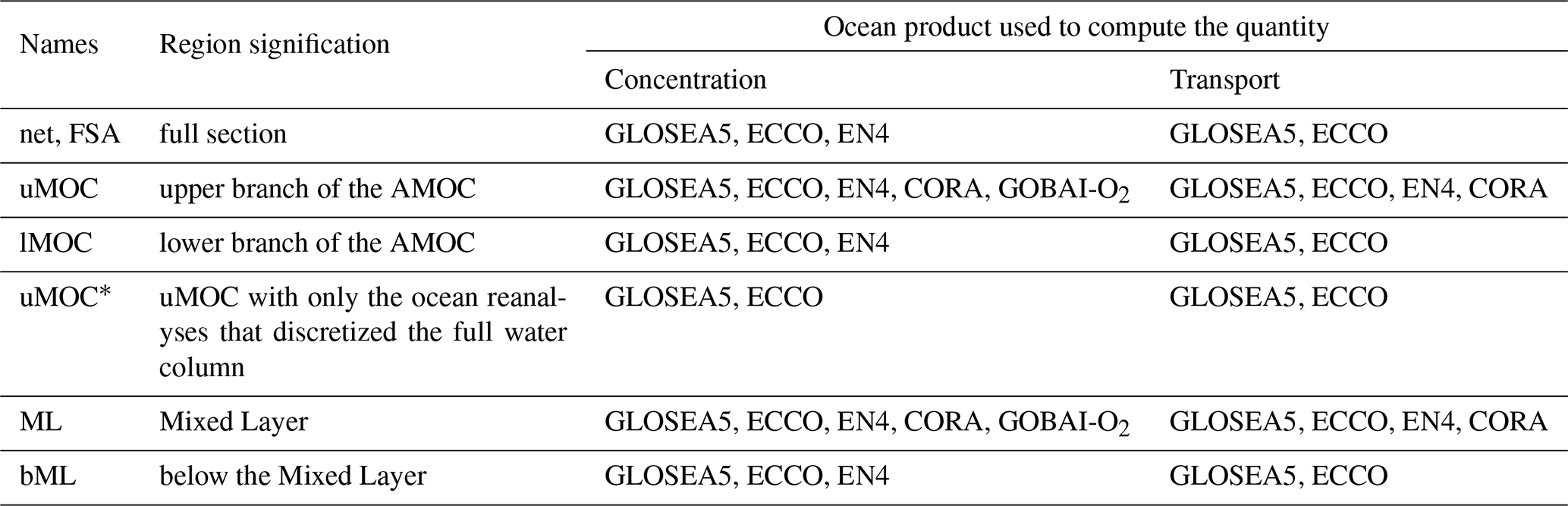
Table 2 Names of the vertical layers and ocean reanalyses used in this study. In the context of transport estimates, a layer denotes the transport across the layer (positive northward). Conversely, in terms of concentrations, it refers to the average concentration over the layer. CORA and GOBAI-O₂ cover the depth range 0–2000 m (Table 1) and their use is therefore limited to the uMOC and mixed-layer (ML) layers. Only GLOSEA5 and ECCO contribute to the calculation of net, lMOC and bML transports. uMOC^* is the average of the uMOC quantity (concentration or transport) over these two ocean reanalyses only.

2.7 Seasonal cycle, interannual filtering, trends and annual profile

From the monthly time series of concentration and transport, seasonal signal time series were obtained by applying a two-year high-pass filter over the time series. The new high-frequency time series were grouped by months and the mean for each month was calculated to derive the seasonal (also referred to as intraannual) signal.

Interannual time series were computed by subtracting the high-frequency time series (obtained using the high-pass filter) from the initial one. The Standard Deviation (SD) of this interannual time series will be used as a metric of interannual variability. In the following, the interannual signal will refer to this low-frequency signal. The standard error (SE) of the average over the reanalyses is defined as the SD between reanalyses divided by the square root of the number of reanalysis used to compute the mean.

Trends are calculated as the slope coefficient of a linear fit. The uncertainty in trends is estimated using the Moving Block Bootstrap method (Kunsch, 1989).

To better quantify the effects of seasonal changes in ML and uMOC thickness on the seasonality of [C_nat] and [C_ant], we calculated an idealized seasonal anomaly for ML and uMOC using the annual mean vertical profile of the property ([C_annual]), rather than monthly varying concentrations, and the full variability of ML depth and uMOC thickness. This approach isolates the impact on ML concentrations of physically-driven seasonal changes in layer thickness from biologically-driven seasonal variations in concentration.

2.8 Error estimation

The error in the estimation of [C_nat] and [C_ant] is the sum of the errors associated with the combined use of ocean reanalyses, NN, and the BC approach. The error associated with the use of NNs is evaluated at the hydrographic section A25, using estimates directly obtained from seawater samples as a reference, first at the sampling points (Sect. 2.8.1) and then for integrated variables such as averaged concentrations (Sect. 2.8.2) and transports (Sect. 2.8.3) in predefined layers. The overall errors resulting from both the use of NN and reanalyses have been estimated altogether for average regional concentrations and transports and comparing them with hydrographic data. The resulting Root Mean Square Deviation (RMSD) give the final errors for integrated concentrations (Sect. 2.8.2) and transports (Sect. 2.8.3), where all errors have been taken into account. The error of the BC approach is fixed according to previous studies to 5.2 µmol kg⁻¹ (Vázquez-Rodríguez et al., 2009; Pérez et al., 2013).

Using error propagation to calculate an error on an integral quantity (e.g., average concentration per layer or property transport by uMOC) would require postulating the error correlation between different variables. This correlation is unknown. Our method of direct comparison with observational results avoids this issue, enabling us to compare final integrated values to reference hydrographic data.

2.8.1 Neural networks evaluation on A25 hydrographic data

The error resulting from the use of NN was quantified by applying NNs to the T and S A25 bottle data to estimate [DIC], and comparing these values to the original [DIC] estimated directly derived from observations (T, S, O₂, nutrients, pH, and A_T bottle data) (Sect. 2.8). The RMSD between both estimates was 9.7 µmol kg⁻¹ (mean for all A25 cruises) for [DIC] (Table S1). The uncertainty of the reference [DIC] from the A25 data is equal to 5.8 µmol kg⁻¹ (see Sect. S1 in the Supplement) and comes from the uncertainties on the measurements of A_T and pH in seawater samples. The RMSD is nearly equal to the median uncertainty of [DIC] of 9.1 µmol kg⁻¹ for CANYON-B-CONTENT (Bittig et al., 2018, see their Table 2). The [O₂] generated by ESPER has a RMSD of 7.8 µmol kg⁻¹ with the A25 bottle (Table S1), which is within the mean uncertainty of 9.1 µmol kg⁻¹ provided in the North Atlantic region by ESPER NN (Carter et al., 2021). The mean uncertainty given by GOBAI-O₂ in [O₂] is 6.3 µmol kg⁻¹ in the SPNA (Sharp et al., 2023). ESPER also retrieves confident nutrient values. For example, nitrate shows an RMSD of 2.8 µmol kg⁻¹ with the A25 data. Applying $\mathit{\phi }{C}_{\mathrm{T}}^{\mathrm{0}}$ on our NN-generated fields (from the initial T, S of the A25 bottle data), we find a RMSD of 5.1 µmol kg⁻¹ for [C_ant] (Table  S1) and 11.3 µmol kg⁻¹ for [C_nat]. Considering that the BC $\mathit{\phi }{C}_{\mathrm{T}}^{\mathrm{0}}$ approach error of 5.2 µmol kg⁻¹ (Vázquez-Rodríguez et al., 2009; Pérez et al., 2013) is independent of that due to the use of NNs for [C_ant], the final error of our [C_ant] estimates is 7.3 µmol kg⁻¹. As highlighted in Asselot et al. (2024), uncertainties in [O₂] and [DIC] may cancel each other out, resulting in relatively low errors on the final [C_ant] values, given uncertainties in [O₂] and [DIC].

The use of [O₂] as an input variable for ESPER NN reduces the error of the predicted variables (Carter et al., 2021; see their Table 10, difference between Eq. (7), including [O₂], and Eq. (8), without [O₂]). The use of ESPER to estimate [O₂] was validated by comparing NN-derived estimates against A25 bottle measurements. [DIC] RMSD increases only marginally when using ESPER-estimated rather than measured [O₂] (9.7 vs. 9.5 µmol kg⁻¹, Table S1), as does [C_ant] RMSD (5.1 vs. 4.7 µmol kg⁻¹, Table S1), supporting the suitability of ESPER for [O₂] estimation in this framework. Hence, the NN predictions at A25 based on T, S are considered sufficiently robust and coherent with respect to the final values of [C_nat] and [C_ant].

Our concentration errors are consistent with those derived from error propagation by Asselot et al. (2024), using 3 Argo-O₂ floats data and a similar NN-based approach. They reported [DIC] and [C_ant] errors of 10.5 and 5.9 µmol kg⁻¹, respectively, compared to 9.7 and 5.1 µmol kg⁻¹ in the present study using reference hydrographic data.

2.8.2 Neural networks applied to ocean reanalyses

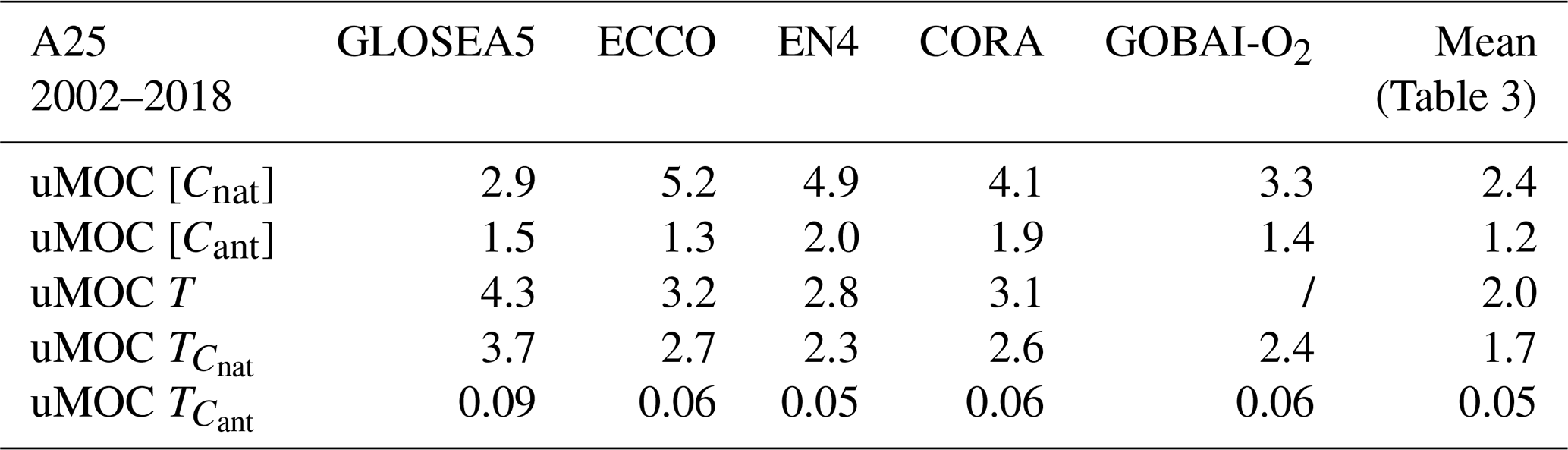
Using ocean reanalysis introduces additional errors stemming from errors in the T and S fields. These errors are included when comparing the section averaged [C_nat] and [C_ant] obtained from OR-NN-BC with the A25 bottle estimates. In this comparison, we compare the synoptic A25 hydrographic sections to the monthly average ocean reanalyses, including the set of errors. We find a RMSD for [C_nat] averaged over reanalyses of 1.4, 2.4, and 1.9 µmol kg⁻¹ for the net, uMOC and lMOC layers, respectively (Tables 3, S2). The RMSD for [C_ant] is of the same order (1.2, 1.2, 0.7 µmol kg⁻¹, for the net, uMOC and lMOC layers, respectively) (Tables 3, S2). Considering the spreading between ocean reanalysis (Tables 4, S3), we find a RMSD for uMOC in the range 2.9–5.2 µmol kg⁻¹ for [C_nat] and 1.4–2.0 µmol kg⁻¹ for [C_ant].

The averaging of the variables reduces the NN errors compared to those calculated for the same variable at the sample points (Tables S1, 3, 4, S2, S3), suggesting that the errors in the concentrations calculated by NNs are mainly random. Examining the differences between the results of the reanalyses and the A25 data, the uMOC biases for [C_nat] range from −3.1 to +4.3 µmol kg⁻¹ depending on the reanalysis with 2.5 to 3.9 µmol kg⁻¹ as SD. For [C_ant] the biases vary from −0.52 to +0.1 µmol kg⁻¹ with 1.3 to 2 µmol kg⁻¹ as SD. Opposite signs in bias reduce RMSD while averaging between reanalyses, especially for [C_nat]. The SDs are of the same order of magnitude as the biases for [C_nat] and greater than the biases for [C_ant].

Table 3 RMSD (for each layer) between [C_nat], [C_ant], $T_{C_{\mathrm{nat}}}$, $T_{C_{\mathrm{ant}}}$ computed with the OR-NN-BC method (mean of all ocean reanalyses) and the estimations derived from the bottle measurements at A25 (2002–2018). The units are µmol kg⁻¹ for concentration and PgC yr⁻¹ for transport of properties. The comparison is made in June for all years in which the A25 cruises were carried out. For the hydrographic section A25, the uncertainties of the transport of the property are calculated with the inverse formalism as in Zunino et al. (2015). The average uncertainty in $T_{C_{\mathrm{nat}}}$ is equal to 2.4, 1.1, 2.0 PgC yr⁻¹ for the net, uMOC and lMOC layers, respectively, while we find 0.04, 0.02 and 0.03 PgC yr⁻¹ for $T_{C_{\mathrm{ant}}}$.

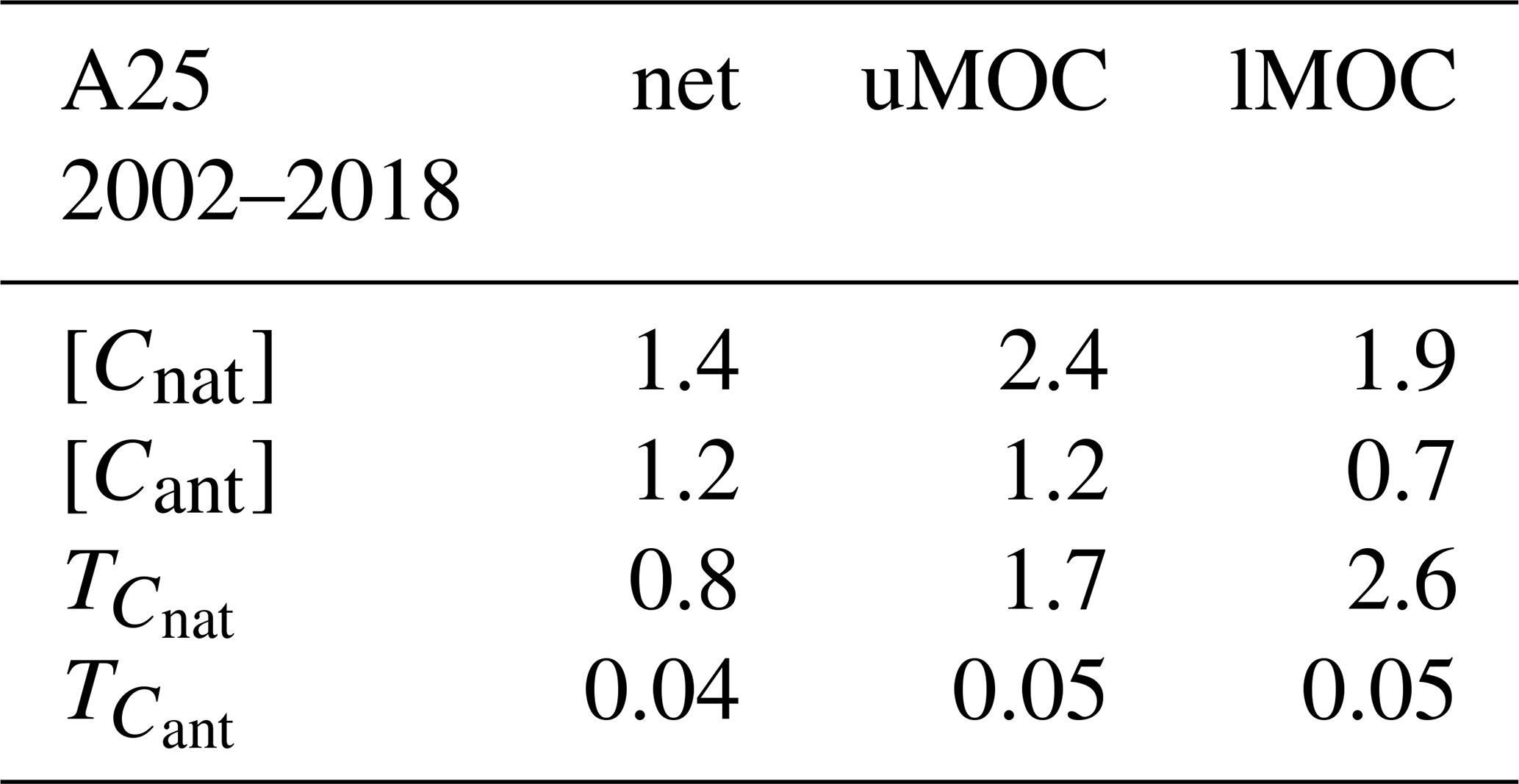
Table 4 RMSD between [C_nat], [C_ant], T, $T_{C_{\mathrm{nat}}}$, $T_{C_{\mathrm{ant}}}$ for the uMOC computed with the OR-NN-BC method (by ocean reanalysis) and the estimations derived from sea bottle measurements at the A25 cruise (2002–2018). The units are µmol kg⁻¹ for concentration, Sv for transport and PgC yr⁻¹ for transport of properties. The comparison is made in June same as above.

2.8.3 Tracer transport

To evaluate the impact of our method on tracer transport estimates, we calculated RMSD between $T_{C_{\mathrm{nat}}}$ and $T_{C_{\mathrm{ant}}}$ calculated with A25 bottle data (Sect. 2.8.1) and those derived from ocean reanalysis using OR-NN-BC (Tables 3, 4, S4). $T_{C_{\mathrm{nat}}}$ presents the RMSD for 2002–2018 of 1.7 PgC yr⁻¹ for the uMOC layer averaged over all reanalyses, while $T_{C_{\mathrm{ant}}}$ presents the RMSD for 2002–2018 of 0.05 PgC yr⁻¹ for the same layer (Tables 3, 4, S4). Both property concentration and volume transport errors are included in this final error estimate, which considers the A25 hydrographic sections as a reference. When calculating RMSD for each ocean reanalysis within the uMOC layer, a range of 2.3–3.7 PgC yr⁻¹ is found for $T_{C_{\mathrm{nat}}}$, and 0.05–0.09 PgC yr⁻¹ for $T_{C_{\mathrm{ant}}}$ (Tables 4, S5). Like for the property, taking the average transport between products also reduces the RMSD within the A25 observations. Using only GLOSEA5 and ECCO (see Table 2), $T_{C_{\mathrm{nat}}}$ presents the RMSD for 2002–2018 of 0.8 and 2.6 PgC yr⁻¹ for the net and lMOC layers, respectively, while $T_{C_{\mathrm{ant}}}$ presents the RMSD for 2002–2018 of 0.04 and 0.05 PgC yr⁻¹ for the same layers, respectively (Table 3).

3 Results

3.1 C_ant and C_nat concentrations

Along the A25 OVIDE section, the C_nat fraction represents, on average, 98 % of the DIC, while the C_ant fraction accounts for only the remaining 2 %. The [C_nat] distribution shows a vertical gradient of generally lower to higher concentrations from surface to depth (Fig. 1), which is largely shaped by the biological carbon pump (Passow and Carlson, 2012). In contrast, the [C_ant] distribution shows an opposite vertical gradient, with the highest concentrations in the upper layers due to direct contact with the atmosphere (Figs. 1, 2). [C_ant] decreases with depth and also from East to West, as the cold subpolar waters contain less [C_ant] than the warmer subtropical waters (Sabine et al., 2004). In particular, the highest [C_ant] signature is found in and east of the North Atlantic Current (NAC) (Fig. 1) which transports C_ant-loaded subtropical waters to higher latitudes. This current represents the primary source of C_ant to the subpolar gyre (Brown et al., 2021; Pérez et al., 2013).

The results discussed in this section are the averages over all reanalyses, unless otherwise indicated. We recall that typical errors of our method on integrated concentration range from 2.9 to 5.2 µmol kg⁻¹ for [C_nat] and from 1.4 to 2.0 µmol kg⁻¹ for [C_ant] (Sect. 2.8).

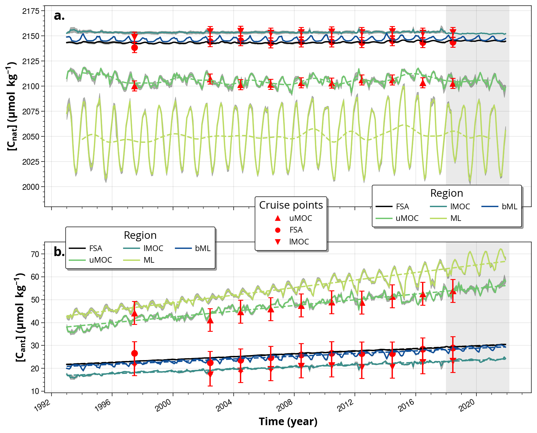
Figure 2 Area mean time series of (a) [C_nat] and (b) [C_ant] in all the layers of interest: the upper and lower branches of the Atlantic Meridional Overturning Circulation (uMOC in green, and lMOC in dark green, respectively), Mixed Layer (ML) in yellow green, and below the ML (bML) in dark blue. The full section averaged concentration (referred to as FSA) is shown in black. For the uMOC and ML layers, the concentration values were computed as the mean of the estimates from GLOSEA5, ECCO, CORA, EN4 and GOBAI-O₂ (Table 2). For the net, lMOC, and bML layers, the concentration values represent the average of the estimates derived from GLOSEA5, ECCO and EN4. The gray shading along the lines represents the standard deviation of all product estimates used in the monthly averaging, divided by the square root of the number of reanalysis. The dashed lines for C_nat (top) represent a low-pass filter time series (cutoff frequency of 24 months). For C_ant (bottom), dashed lines indicate the linear trend. The A25 cruise [C_nat] and [C_ant] estimates for uMOC, lMOC, and net are shown in red, with red vertical lines denoting the error bars. The grey shading at the end of the time series highlights the period for which only the GLOSEA5 reanalysis is available.

3.1.1 Seasonal

The amplitude of the [C_nat] seasonal cycle is the highest for ML (Figs. 2, 3b). We find a maximum positive anomaly of 32.1 ± 1.4 µmol kg⁻¹ in March and a maximum negative anomaly of −37.1 ± 1.9 µmol kg⁻¹ in August (Fig. 3b). The seasonal variability of [C_nat] in ML (ML [C_nat] hereafter) may be due to the seasonal variations of both [C_nat] and the ML depth (as it deepens, the ML incorporates higher values of [C_nat]). To better understand the effect of varying the ML depth, we calculated the effect that the seasonality in ML depth applied to an annual mean [C_nat] profile would have (Fig. 3b, see Sect. 2.7), the difference between the two being related to the seasonality of the biological activity. We observe that seasonal variations in the ML depth account for approximately two–thirds of the seasonal ML [C_nat] amplitude in March, and only up to one-third in August (Fig. 3b). All ocean reanalyses show a deepening of the ML in winter (Fig. S2) so that the deep layers with higher [C_nat] have a greater contribution to ML [C_nat]. The deepening is more pronounced in the Irminger Sea (IS) than in the NAC (Iceland Basin) or east of the NAC (Iberian Basin) (Fig. S3) which, combined with the downward increase in [C_nat], explains that the amplitude of the ML [C_nat] seasonal cycle is larger in the IS (70.6 µmol kg⁻¹) than in the NAC (60.2 µmol kg⁻¹).

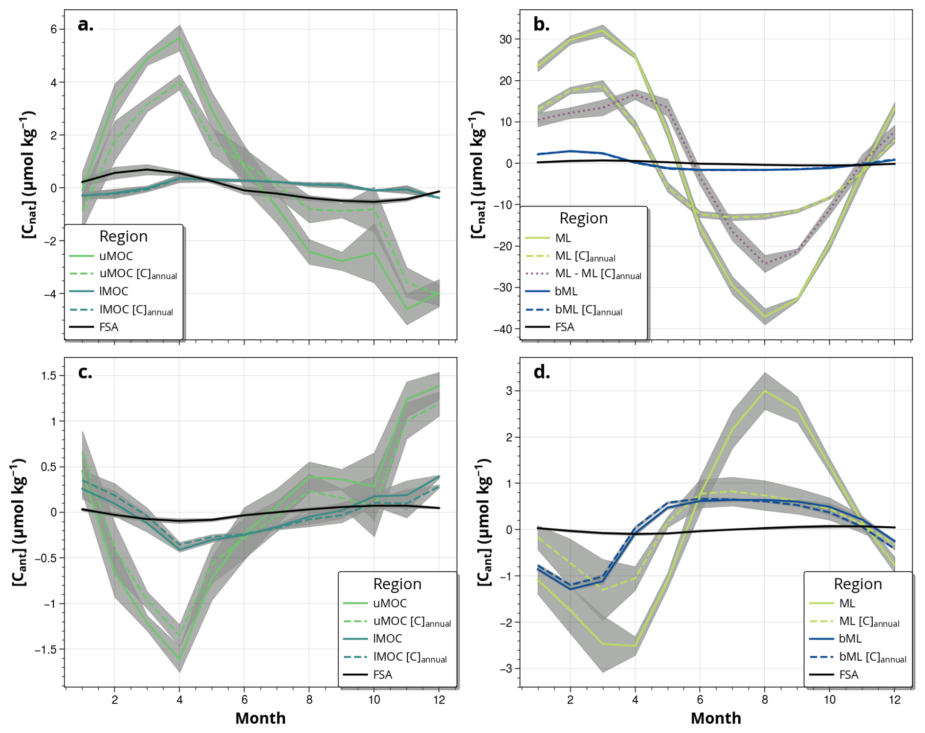
Figure 3 (a, b) Natural carbon [C_nat] and (c, d) anthropogenic carbon [C_ant] seasonal anomalies. Left (a, c) and right (b, d) panels show respectively uMOC/lMOC and ML/bML (Fig. 1, Table 2). Black lines represent the full section-average (referred to as FSA in the legend), light colors are used for the layers the closest to the sea surface (uMOC and ML), and dark colors account for the deeper layers (lMOC and bML). Each monthly value represents the mean value calculated from the ensemble of ocean reanalyses, and the shaded areas the standard errors. The dashed lines represent the idealized seasonal anomaly computed using annual mean property fields and only taking into account changes in area surfaces of layers (see Sect. 2.7 for details). The difference between the seasonal cycle of [C_nat] in the ML and its idealized anomaly, attributed to biological activity, is shown in purple (b).

The seasonal cycle of uMOC [C_nat] varies in phase with the seasonal cycle of ML, but is six times lower (Fig. 3a, b). A maximum positive anomaly of 5.7 ± 0.5 µmol kg⁻¹ is observed in April, and a maximum negative anomaly of −4.6 ± 0.6 µmol kg⁻¹ in November (Fig. 3a). As for the ML, the seasonal cycle of uMOC [C_nat] appears to be related to changes in the surface area of uMOC and changes in the biological pump. Consistent with the downward increase in [C_nat], the maximum (minimum) thickness of the uMOC in April (fall) (Fig. S2) corresponds to the maximum (minimum) [C_nat] (Figs. 1, 4c). Quantifying the proportion of seasonality related to biological activity, a maximum difference is observed in March–April (1.7 µmol kg⁻¹) and September (1.9 µmol kg⁻¹). Mercier et al. (2024) showed that the thickness of the uMOC varies seasonally in opposite directions in the IS compared to the rest of the section, decreasing (increasing) in winter (summer) in the IS, but increasing (decreasing) in the eastern part of the section. Figure 4c shows that the amplitude of the seasonal cycle for uMOC [C_nat] in the IS is markedly different from the rest of the section. Although the maximum anomaly observed in April is in phase with the rest of the section, there is a pronounced minimum in August that we relate to maximum biological activity (see, e.g., Lacour et al., 2015). This suggests that seasonal changes in the uMOC [C_nat] in the IS depend more than the rest of the section on biologically-driven changes.

Smaller seasonal variations are observed in the lMOC and bML layers (of 0.7 and 4.6 µmol kg⁻¹, respectively), which can be interpreted as these layers being less affected by seasonal forcing due to their greater distance from the surface (Fig. 3). Despite their small magnitudes, the signals remain significant due to the small associated SD. The amplitude of the full section-average seasonal [C_nat] anomaly of 1.2 µmol kg⁻¹ is largely determined by these low-amplitude signals of lMOC and bML, as these layers occupy a greater surface area.

As for [C_nat], the seasonality of [C_ant] is the highest in ML and the second highest in the uMOC (Fig. 3c, d). The [C_ant] values are minimal when [C_nat] is maximal and vice versa (Figs. 3, 4). A positive [C_ant] anomaly of 3.0 ± 0.4 µmol kg⁻¹ and a negative [C_ant] anomaly of −2.5 ± 0.2 µmol kg⁻¹ are observed in August and April, respectively, hence a 5.5 µmol kg⁻¹ seasonal amplitude (Fig. 3). Following the same approach as for [C_nat], we note that the seasonal variation in thickness of the ML applied to an annual mean [C_ant] profile explains at most a third of the ML [C_ant] seasonal signal (Fig. 3d). The latter can be explained by the Revelle factor that creates seasonality in the surface [C_ant]. The Revelle factor decreases (increases) with increasing (decreasing) temperature, and the surface [C_ant] follows the temperature seasonal cycle with a peak-to-peak amplitude of about 4 µmol kg⁻¹ (Fig. S4), in phase with that caused by the ML depth seasonal cycle. In all regions, the cooling and winter deepening of ML decrease ML [C_ant] due to the lower concentration at depth and larger Revelle factor (Fig. 4).

With a minimum in April (−1.6 ± 0.1 µmol kg⁻¹) and a maximum in December (+1.4 ± 0.1 µmol kg⁻¹), the peak-to-peak seasonal amplitude of uMOC [C_ant] is 3.0 µmol kg⁻¹ and approximately half that of ML [C_ant] (Fig. 3c). We note that the variation in thickness of the uMOC applied to an annual mean [C_ant] profile explains most of the seasonal [C_ant] uMOC signal (Fig. 3c). Regionally, the deepening of the uMOC in winter in the NAC (see Mercier et al. (2024)) decreases the uMOC [C_ant] (Fig. 4d). The reverse holds for summer, when the volume of uMOC decreases in the NAC. In the IS, a different mechanism prevails. The uMOC is confined to the surface layer and essentially belongs to the ML. The seasonal cycle of [C_ant] is therefore similar to that of ML [C_ant] and not the one we would expect, given that the thickness of the uMOC is less in winter than in summer (Mercier et al., 2024) (Fig. 4).

The bML and lMOC layers have reduced seasonal signals. The summer-to-winter difference is equal to 1.9, 0.8 µmol kg⁻¹ for the bML, lMOC, respectively. The seasonal amplitude of the full section averaged is negligible (+0.2 µmol kg⁻¹ between April and October).

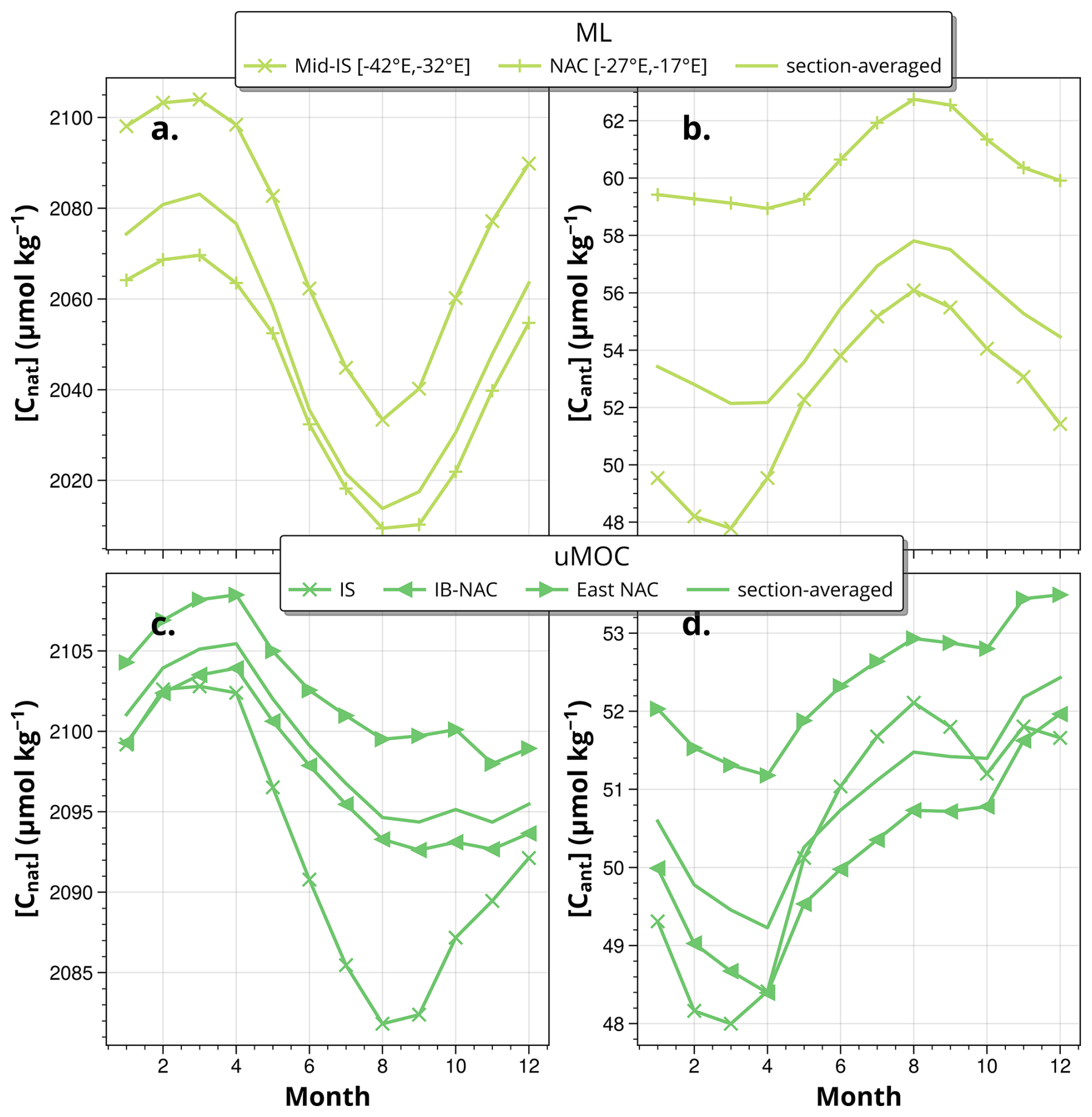
Figure 4 Seasonality of (a) ML [C_nat] and (b) ML [C_ant] for the full section (continuous color line), the center of Irminger Sea (between −42 and −32° E, line with x markers) and the NAC (between −27 and −17° E, line with + markers). Seasonality of (c) uMOC [C_nat] and (d) uMOC [C_ant] for the full section (continuous color line), the Irminger Sea (line with x markers), the Iceland Basin-NAC region (IB-NAC) (line with ◂ markers) and the East of the NAC (line with ▸ markers). The seasonal cycles are obtained by grouping the time series data by month and averaging over all ocean reanalyses. The time series are subsets of the complete series of Fig. 2, sampled from 2004 to 2017, so that each reanalysis has the same weight in the construction of the seasonality (Table 1).

3.1.2 Interannual to long-term

As evidenced by the time series in Fig. 5a, the interannual variability in [C_nat] is characterized by a 4–6 year periodic signal in the uMOC and, although a little less clear, in the ML (Fig. 5a). The peak-to-peak amplitude of the signal ranges from 8.5 to 11.2 µmol kg⁻¹ in the uMOC and from 7.5 to 14.6 µmol kg⁻¹ in the ML (Fig. 5a). Considering the SD of the mean ML and uMOC [C_nat] values (±SD) for the whole period 1993–2022 (3.6 and 2.9 µmol kg⁻¹, for a mean value of 2050.3 and 2105.9 µmol kg⁻¹, respectively), along with the method uncertainty (2.4 µmol kg⁻¹ for the uMOC) (see Table 3), we conclude that the signal is statistically significant.

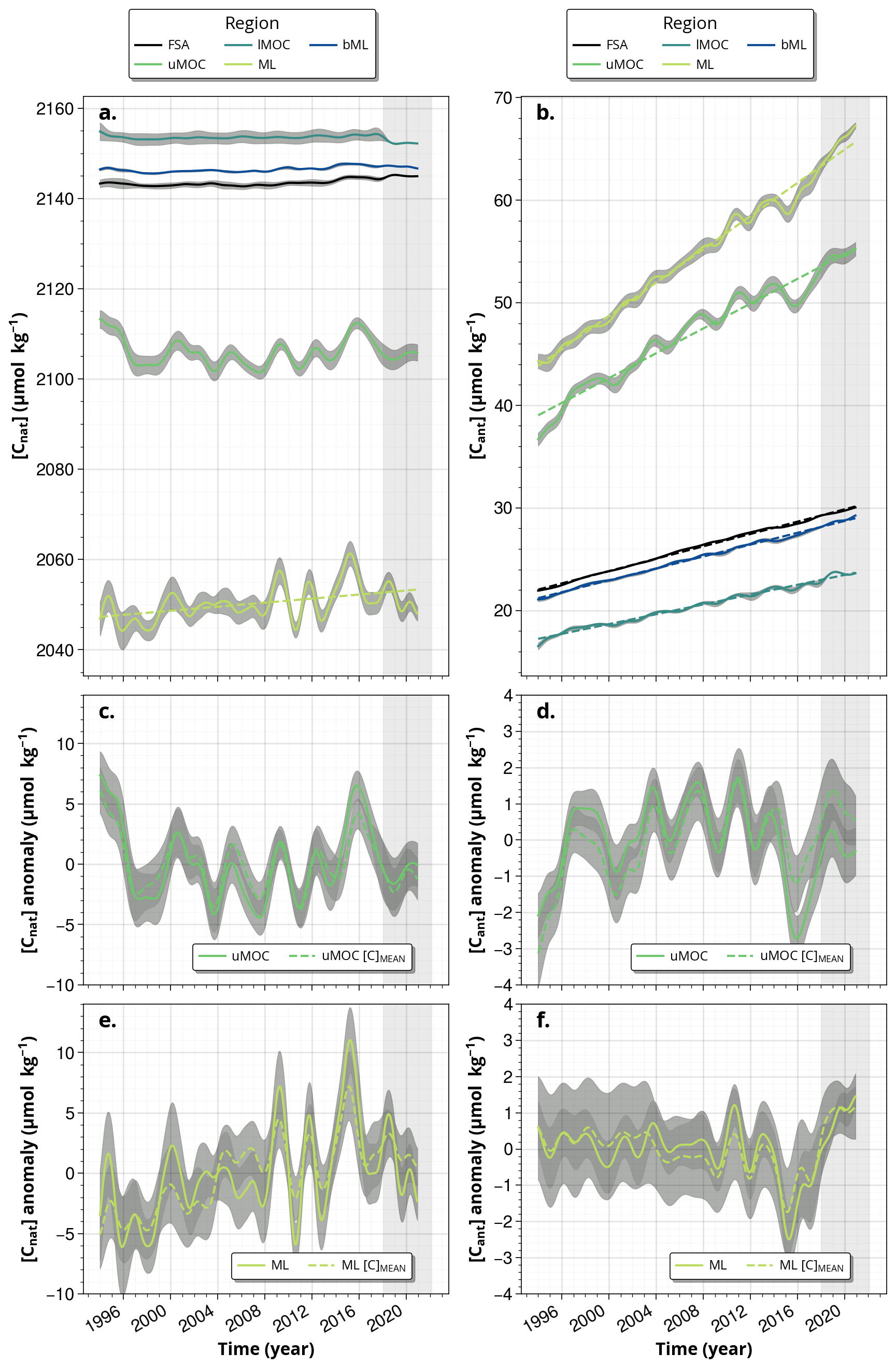
Figure 5 Low pass filtered signal (continuous lines) with their linear trends (dashed lines, plotted when significant at the 90 % significance level) of (a) [C_nat] and (b) [C_ant] in the layers of interest uMOC, lMOC, ML and bML based on time series reported in Fig. 2. Full section average (FSA) concentration is in black. For the uMOC (c, d) and (e, f) ML, the signal is plotted in an anomaly along with the corresponding signal for a mean concentration [C]_MEAN. For [C_ant], the linear trends have been removed in the anomaly plots. Grey shading indicates when only GLOSEA5 reanalysis is available. SEs (±) are shown in grey shading. Linear fit (± confidence interval at 90 %) on interannual [C_nat]: 0.22 ± 0.04 µmol kg⁻¹ yr⁻¹ (ML). Linear fit values on interannual [C_ant]: 0.8 ± 0.008 µmol kg⁻¹ yr⁻¹ (ML), 0.3 ± 0.002 µmol kg⁻¹ yr⁻¹ (bML), 0.6 ± 0.012 µmol kg⁻¹ yr⁻¹ (uMOC), 0.3 ± 0.002 µmol kg⁻¹ yr⁻¹ (lMOC) and 0.3 ± 0.001 µmol kg⁻¹ yr⁻¹ (FSA).

These quasiperiodic changes in [C_nat] are in phase with the changes in the average depth of the ML and the thickness of the uMOC (Fig. S2), and not strongly correlated to the North Atlantic Oscillation (pearson coefficient of 0.32 for interannual uMOC [C_nat] and 0.55 for interannual ML [C_nat]). We have plotted in Fig. 5c, e the interannual variability of [C_nat] due solely to variations in the depth of ML and the thickness of the uMOC, obtained using [C_nat] averaged over the total duration of the time series. Variability due to changes in uMOC thickness and ML depth explain most of the interannual variability in [C_nat]. This is further illustrated in Figs. S3 and S5 from GLOSEA5, which show that a maximum in the surface section area is associated with a maximum in [C_nat]. In the ML, the interannual signal in the section area is dominated by the varying maximum depth of the winter ML (Fig. S2), that is, the interannual variability in seasonal processes (such as the winter ML mixing) causes interannual concentrations to vary. The deep ML observed in the IS in winter 2015 and 2016 appears to have had the most significant impact on interannual variability of ML [C_nat] (Fig. S3). The interannual changes in the area of the uMOC layer are the greatest in the West European Basin (Fig. S5), where the interannual changes in σ_MOC density results in uMOC thickness variations (Mercier et al., 2024), impacting interannual uMOC [C_nat]. Regarding long-term changes, the uMOC [C_nat] does not show any significant tendency. In contrast, the ML shows a significant increase in its variability from 2008 onward. It is concomitant with the intermittent resumption of deep convection in the NASP and documented events in 2008, 2012 and 2015 (Piron et al., 2016, 2017) associated with maxima of [C_nat] creating an apparent [C_nat] (linear) increase of 0.22 ± 0.01 µmol kg⁻¹ yr⁻¹ over the period (Fig. 5a). lMOC and bML [C_nat] did not show interannual variability and no trends. These layers have the largest [C_nat] mean values (2153.4 ± 0.5 µmol kg⁻¹ and 2146.5 ± 0.6 µmol kg⁻¹ for lMOC and bML, respectively) and the largest surface section areas. They contribute the most to the section average mean [C_nat], mostly constant over 1993–2022, which shows no interannual variability and no trend, with a mean value (±SD) of 2143.5 ± 0.8 µmol kg⁻¹ (Fig. 5).

Unlike [C_nat], [C_ant] is dominated by the long-term signal across all layers considered (Fig. 5). The ML shows the highest mean [C_ant], and the highest rate of [C_ant] increase of 0.825 ± 0.016 µmol kg⁻¹ yr⁻¹ (Fig. 5b). It is followed by the uMOC, with a [C_ant] increase rate of 0.625 ± 0.027 µmol kg⁻¹ yr⁻¹ (increase in [C_ant] uMOC of 45.6 ± 2.0 % from 38.4 to 55.9 µmol kg⁻¹ between 1993 and 2021). However, lMOC, not highly concentrated in [C_ant], experiences the same relative increase in [C_ant] of 40.2 ± 0.7 % (which increased from 17.0 to 23.9 µmol kg⁻¹ between 1993 and 2021 at a linear rate of 0.245 ± 0.005 µmol kg⁻¹ yr⁻¹) as bML and section average. In terms of the section average [C_ant], the increase rate is 0.301 ± 0.004 µmol kg⁻¹ yr⁻¹, with a mean [C_ant] value varying from 21.7 µmol kg⁻¹ in 1994 to 30.4 µmol kg⁻¹ in 2021. For [C_ant], the interannual variability is mainly observed in ML and uMOC, similar to [C_nat], although in opposite phases due to inverse vertical concentration gradients. The amplitude of the interannual signal ranges from 0.7 to 3.4 µmol kg⁻¹ for the ML, and from 2.6 to 3.9 µmol kg⁻¹ for the uMOC. These values lie above the method's error (1.2 µmol kg⁻¹ for uMOC [C_ant], Table 3).

3.2 C_ant and C_nat transports

The time series of volume, C_nat and C_ant transports across A25 for each of the ocean reanalysis are presented in Fig. 6, with independent cruise-based estimates shown in red.

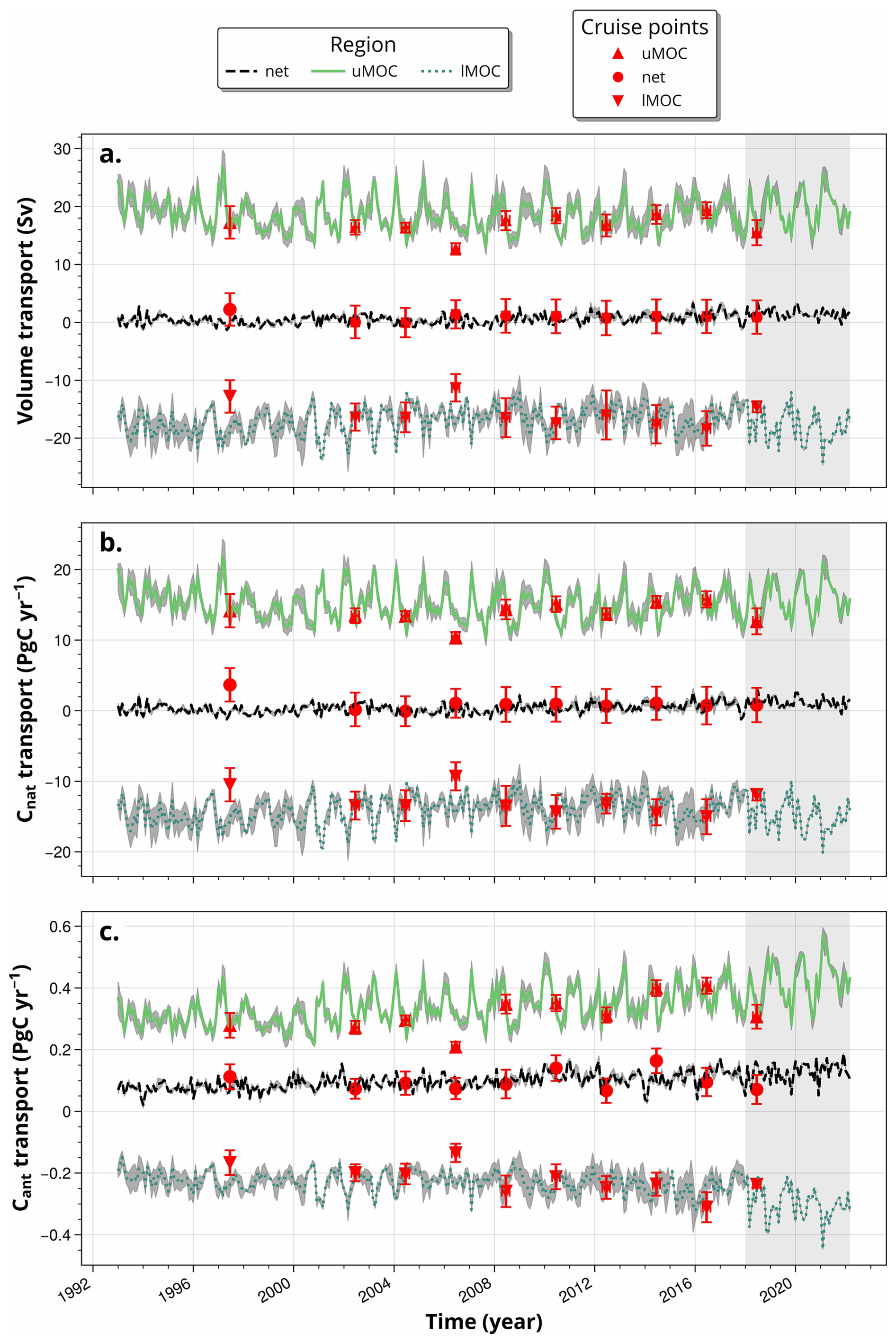
Figure 6 (a) Volume, (b) C_nat and (c) C_ant transports. Each panel (a, b, c) shows the net transport value across A25 (average of ECCO and GLOSEA5), the uMOC transport (average of ECCO, GLOSEA5, EN4, CORA transports) and the lMOC transport (average of ECCO and GLOSEA5). The standard errors (SEns) for the mean values computed as the SDs divided by the square root of the number of reanalysis are shown as grey shading. The cruise estimates with their uncertainties indicated in red are from Daniault et al. (2016); Lherminier et al. (2007, 2010); Zunino et al. (2014, 2015, 2017); Mercier et al. (2024). Vertical grey shading indicates when only the GLOSEA5 reanalysis is available.

3.2.1 Seasonal

Maximum seasonal northward C_nat transport anomalies of 2.66 and 2.63 PgC yr⁻¹ are observed in March within uMOC and ML, respectively (Fig. 7c, d). The seasonal anomaly of uMOC C_nat transport reaches a minimum of −1.80 PgC yr⁻¹ in September. Between June and November, the ML C_nat transport anomaly is negative with a slight minimum of −1.19 PgC yr⁻¹ in June. uMOC^* C_nat transport seasonality is dampened compared to uMOC while ML^* C_nat transport seasonality is strengthened compared to that of ML. The seasonality of the transport of lMOC (bML) C_nat is the opposite to that of uMOC^* (ML^*) C_nat transport seasonality. C_nat transport in the lMOC reaches a −1.24 PgC yr⁻¹ maximum to the South in March and a 1.15 PgC yr⁻¹ maximum to the North in September and November (Fig. 7c). C_nat transport in the bML reaches −4.06 PgC yr⁻¹ to the South in March and a maximum seasonal anomaly to the North of 2.11 PgC yr⁻¹ in September (Fig. 7d). The seasonal anomaly of net C_nat transport is minimum in May (−0.28 PgC yr⁻¹) and maximum in September (0.34 PgC yr⁻¹) (Fig. 7c, d). Its amplitude is an order of magnitude lower than the seasonal anomaly of the uMOC, lMOC, ML and bML layers.

The seasonality of C_ant transport is mainly in phase with the seasonality of C_nat transport (Fig. 7c–e, d–f). In the uMOC, there is a corresponding northward maximum of 0.06 PgC yr⁻¹ in March and a reduced southward transport in September of −0.04 PgC yr⁻¹ (Fig. 7e). The seasonality of uMOC^* C_ant transport is dampened compared to that of the uMOC. The seasonality of the transport of ML C_ant is slightly higher than that of uMOC in the late winter, with 0.08 PgC yr⁻¹ to the North in March (Fig. 7f). There is a rapid drop in April in the transport of ML C_ant and a negative anomaly of −0.04 PgC yr⁻¹ in July, corresponding to half of the maximum ML in late winter (Fig. 7f). The seasonality of ML^* C_ant transport is slightly larger than that of ML C_ant transport. The transport of bML C_ant is equal to −0.09 PgC yr⁻¹ southward in March and shows a plateau between June and November of almost 0.05 PgC yr⁻¹ (Fig. 7e). The net C_ant transport seasonality is very small. Seasonal net C_ant transport is influenced by both the seasonal variation of net volume transport and full section averaged concentration (Figs. 7a, b and 3c, d).

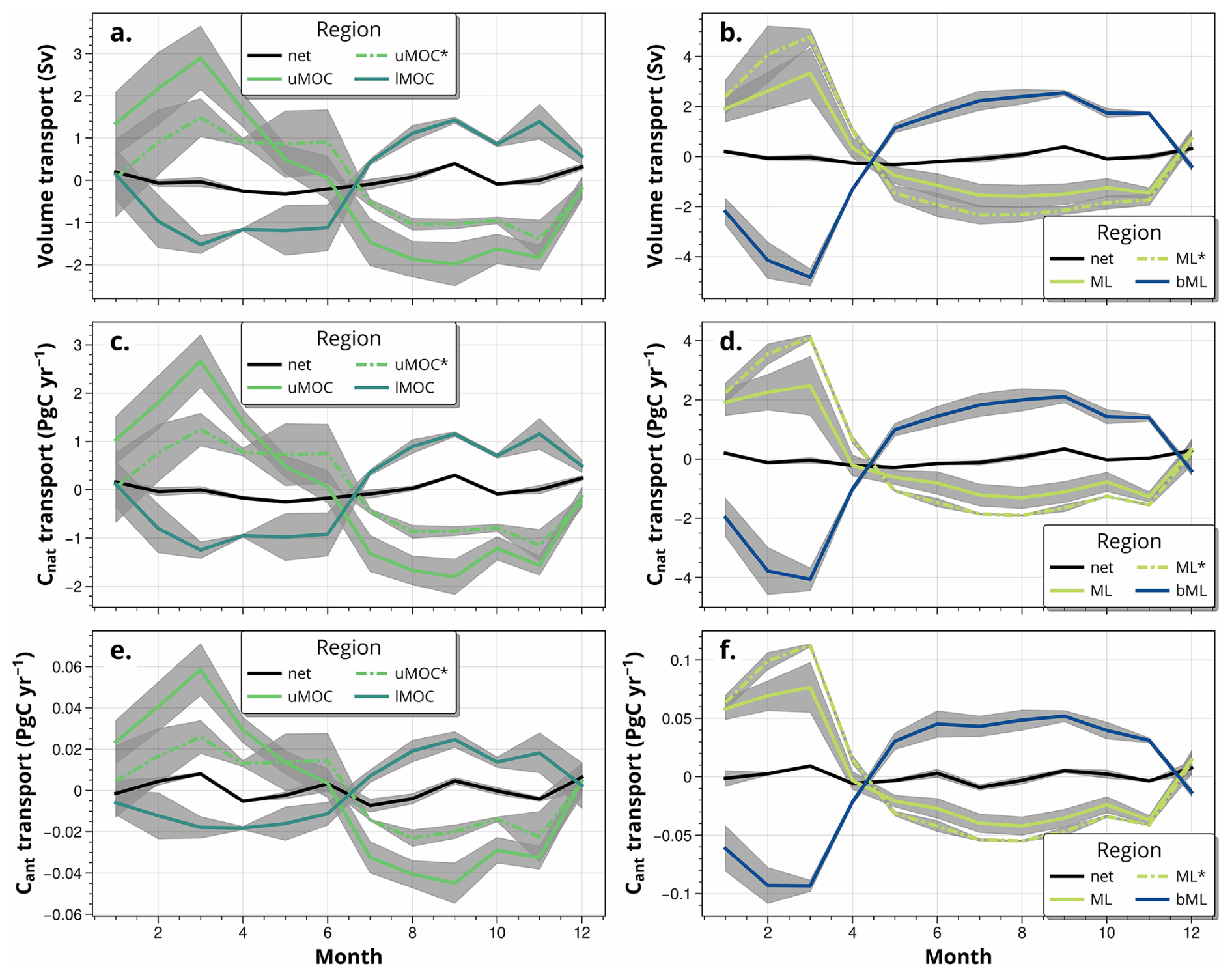
Figure 7 Volume (a, b), C_nat (c, d), and C_ant (e, f) seasonal transport anomalies. Left (right) panels show uMOC/lMOC (ML/bML). Light colors represent the upper-ocean layers (either uMOC or ML), dark colors the deeper-ocean layers (either lMOC or bML), and the black lines the net transport (section integration). The seasonal anomalies presented here are computed using the average of all reanalyses available. uMOC^* and ML^* represent the average of only GLOSEA5 and ECCO, to align with the lMOC and bML estimates, which are based solely on these two datasets (Table 2). The shaded areas is the standard error for the mean (SEn) computed as the standard deviation for each month, divided by the square root of the number of reanalysis.

The seasonal cycle of the C_ant and C_nat transports closely reflects the seasonality of the volume transport, as evidenced by the similarity between the seasonal cycles of the volume transport and the property transport (Fig. 7). The strong influence of ocean circulation on the seasonal transport of C_ant and C_nat is also supported by the fact that, for a given layer (ML or MOC branches), although [C_nat] and [C_ant] seasonal anomalies are opposite, C_nat transport and C_ant transport seasonal signals are synchronous (Fig. 7). The seasonal variations of volume transport of 4.88 and 2.95 Sv for uMOC and lMOC, respectively, represent 26.1 % and 17.3 % of their annual mean values corresponding to seasonal changes of 4.46 and 2.40 PgC yr⁻¹ for C_nat, and 0.10 and 0.04 PgC yr⁻¹ for C_ant for uMOC and lMOC, respectively (Fig. 7). The seasonal amplitudes for the uMOC and the lMOC for the transport of C_nat (C_ant) represent 29.3 % and 17 % (29.8 % and 17.9 %) of their annual mean value (Figs. 6a, c and 7a, e). The sole observed effect of the seasonality of [C_ant] is on the seasonality of the net C_ant transport.

3.2.2 Interannual to long-term

The net volume transport along the section is close to 1 Sv for the 30-year time series, the uMOC and lMOC transports having opposite signs (Fig. 6). These opposite signs will be reflected in the signs of uMOC and lMOC C_nat (C_ant) transports (Figs. 6, 8).

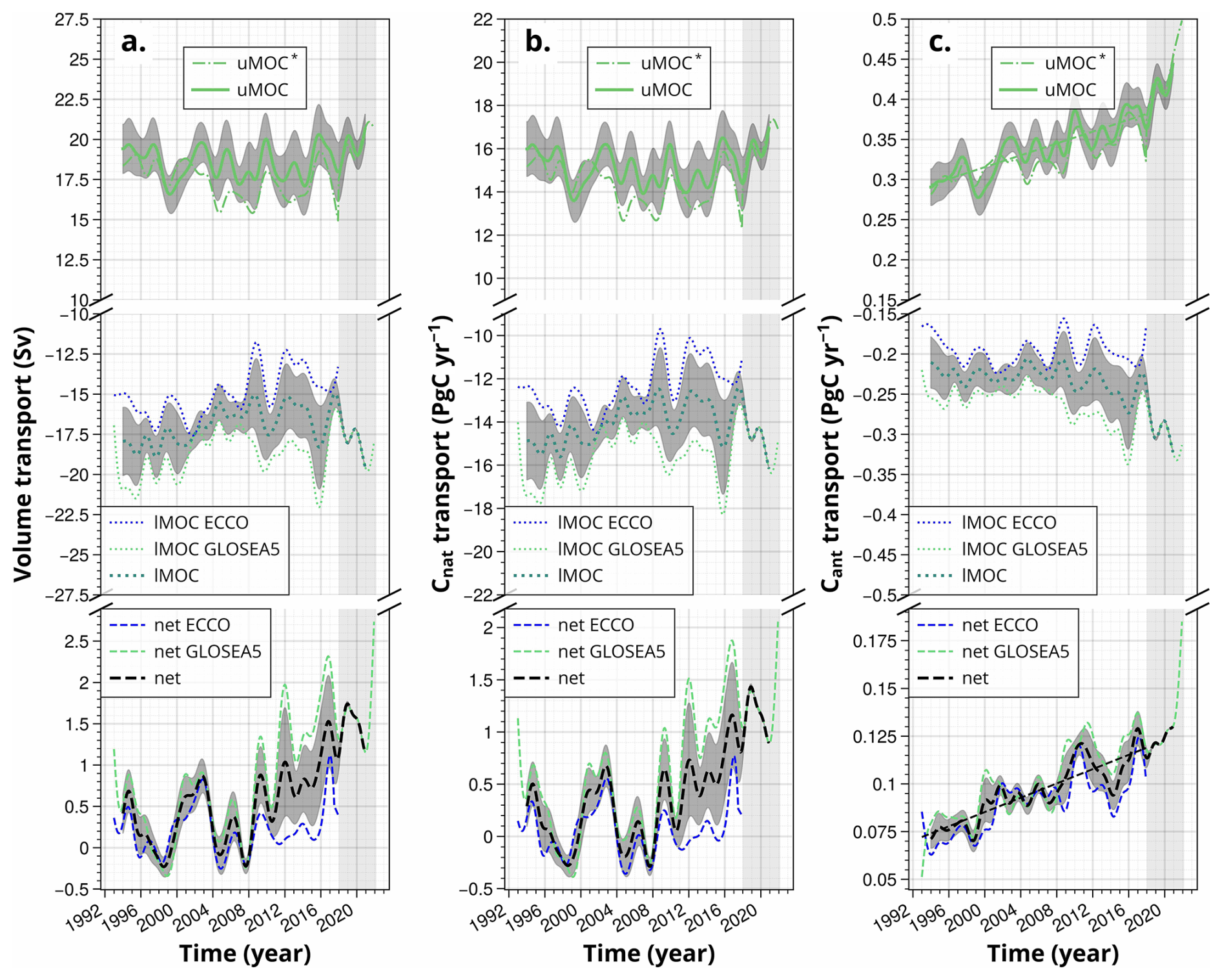
Figure 8 Low-pass filtered (a) volume, (b) C_nat and (c) C_ant transports time series for the uMOC (upper panels), lMOC (middle panels) and net section (bottom panels). These interannual time series were obtained by subtracting the high frequency time series obtained using a one-year high-pass filter to the original series, as reported in Fig. 6 (see Sect. 2.7). The dashed straight lines correspond to the linear trends on the low-pass filtered signals. Vertical light grey shading indicates where only GLOSEA5 reanalysis is available. The standard errors (SEns) are shown in dark grey shading for the mean values.

The net C_nat transport averages to 0.40 ± 0.44 PgC yr⁻¹ northward over 1993–2021 (Fig. 8b). This transport did not show a tendency before 2010 and increased from 0.13 ± 0.15 to 1.04 ± 0.09 PgC yr⁻¹ between 2010 and 2021 (Fig. 8b). The SE of the net C_nat transport increases over time, from 0.18 PgC yr⁻¹ for 1993–2010 to 0.33 PgC yr⁻¹ for 2011–2018. Between 1993 and 2021, the C_nat transports for the uMOC and lMOC average to 15.3 ± 1.1 and −14.1 ± 1.1 PgC yr⁻¹, respectively. There is noticeable variability in C_nat uMOC transport with a longer-term weakening period before 2010 and growth after this year. In 2021, uMOC C_nat transport reaches 17.78 ± 0.63 PgC yr⁻¹ (Fig. 8b). The C_nat uMOC and lMOC transports show the same variability as the uMOC and lMOC volume transport (Fig. 8a, b). The reduction of 1.15 (1.94) Sv in the volume transport of uMOC (lMOC) between the 1993–1997 pentad and the 2008–2012 pentad results in a decrease of 1.17 (1.58) PgC yr⁻¹ in the C_nat uMOC (lMOC) transport during the same period (Fig. 8a, b). This result indicates that the interannual variations of [C_nat] are negligible compared to volume changes (Figs. 3b, 8a). Pearson coefficient correlation of 0.98 (0.99) is found between interannual volume and C_nat transport in the uMOC (lMOC), highlighting that changes in volume transport outweigh changes in concentration. The interannual variability of uMOC C_nat transport amounts to 0.86 PgC yr⁻¹ (uMOC SD in Fig. 8b). It is an order of magnitude smaller than the seasonal amplitude of transport of uMOC C_nat (4.46 PgC yr⁻¹). The dispersion between ocean reanalysis C_nat transport is measured by SEns. The uMOC SEns average at 1.06 PgC yr⁻¹ for 1993–2021. A larger dispersion in the reanalyses is observed within the C_nat lMOC transport after 2010, the SEs increasing from 1.15 PgC yr⁻¹ for 1993–2010 to 1.36 PgC yr⁻¹ for 2011–2018. Breaking down the net interannual C_nat transport time series following Eq. (3), we note that most of the variability is explained by the net' C_nat transport i.e. the product at each time step of the net volume transport by the average property. This is confirmed in Fig. 9 where 99 %–100 % of the C_nat transport variance (r²) is explained by net' C_nat transport and thus volume transport variability for ECCO and GLOSEA5, respectively. The variability of C_nat transport in the SPNA at A25 is shown to be driven by volume transport both in the uMOC, lMOC and net sections at the interannual and long-term time scales (Figs. 6–8).

The net C_ant transport doubled in thirty years, from 0.07 in 1993 to 0.14 PgC yr⁻¹ in 2021 northward corresponding to an increase of 0.023 PgC per decade. Its evolution is closely approximated by a linear increase (Fig. 8c). C_ant transport in the uMOC increased from 0.29 ± 0.03 to 0.45 ± 0.02 PgC yr⁻¹ between 1993 and 2021 (0.056 PgC per decade). In contrast, the lMOC C_ant southward transport shows no trend until 2008, after which it increases. This results in an overall increase between 1993 and 2021 from −0.19 ± 0.03 to −0.32 ± 0.04 PgC yr⁻¹ (0.047 PgC per decade, Fig. 8c). The southward transport of lMOC compensates in part for the northward transport of uMOC. The relative increase in [C_ant] in uMOC is close in percentage (45.6 ± 2.0 %, 48.4 ± 2.6 % for uMOC^*) to that in lMOC (37.4 ± 0.7 %) (Fig. 5). However, the net northward [C_ant] transport increases due to higher [C_ant] values in the upper layers and an increase in the difference in [C_ant] between uMOC and lMOC from 1994 to 2021, uMOC [C_ant] being 19 % larger than lMOC [C_ant] in 1993 but more than twice in 2021 (Fig. 5). The section averaged [C_ant] shows an increase of 9.1 µmol kg⁻¹ (42.5 ± 0.8 %) between 1993 (21.4 µmol kg⁻¹) and 2021 (30.5 µmol kg⁻¹) (Fig. 5b). For the net C_ant transport, there is a first period of small increase before 2010, which is resulting from an increase in [C_ant] compensated for by a decrease in the water mass transport over the period (Figs. 5a and 8c) for both branches. After 2008, the increase is more rapid, with a rate of 0.038 PgC per decade compared to 0.013 PgC per decade previously, as both volume transport and concentration are intensified. The interannual C_ant transport for uMOC and lMOC follows the interannual transport of volume (Fig. 8). Pearson correlation coefficients of 0.91 and 0.93 were obtained between the two interannual transports for uMOC and lMOC, respectively.

The large correlations between the diapycnal component (Eq. 3) and the net C_ant transport (r² values of 0.71, 0.81 for ECCO, GLOSEA5) (Fig. 9c, d) show that the diapycnal component T_diap drives the net C_ant transport. The strong positive T_diap for C_ant comes from the higher concentration of C_ant in uMOC than in lMOC (Fig. 5b). Separating the two components of the diapycnal transport (velocity and [C_ant]) into a time-mean term (overline) and a fluctuation term (prime) in Fig. 10 shows that the interannual changes in diapycnal transport come from the changes in volume and velocity multiplied by the average concentration of [C_ant], for both GLOSEA5 and ECCO (Fig. 10).

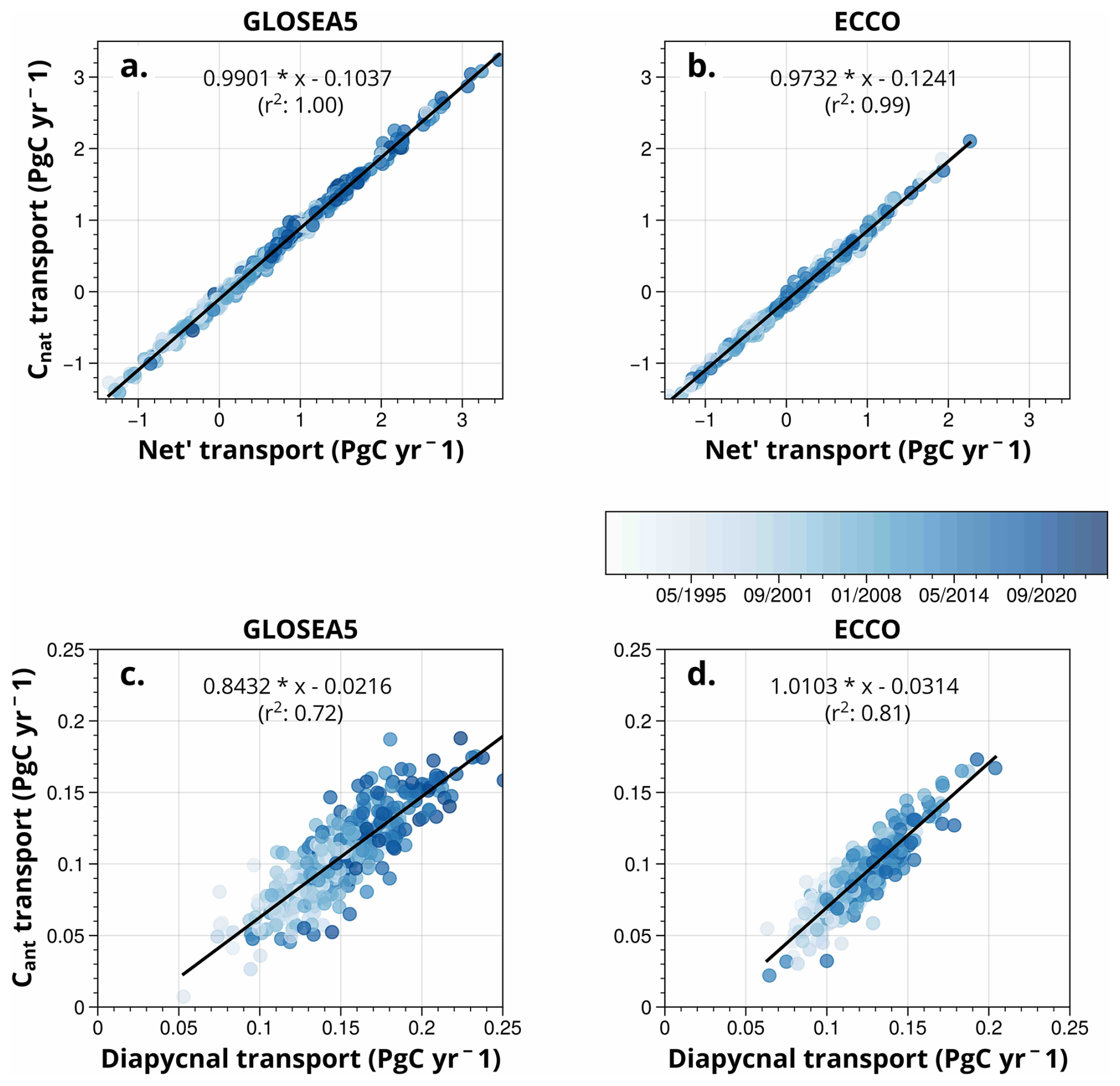
Figure 9 (a, b) Natural carbon (C_nat) transport as a function of its net' term along with the (c, d) anthropogenic carbon (C_ant) transport as a function of its diapycnal term, for (a, c) GLOSEA5 and (b, d) ECCO. The data points are colored according to their date. The linear function with the r² coefficient is shown on the figures.

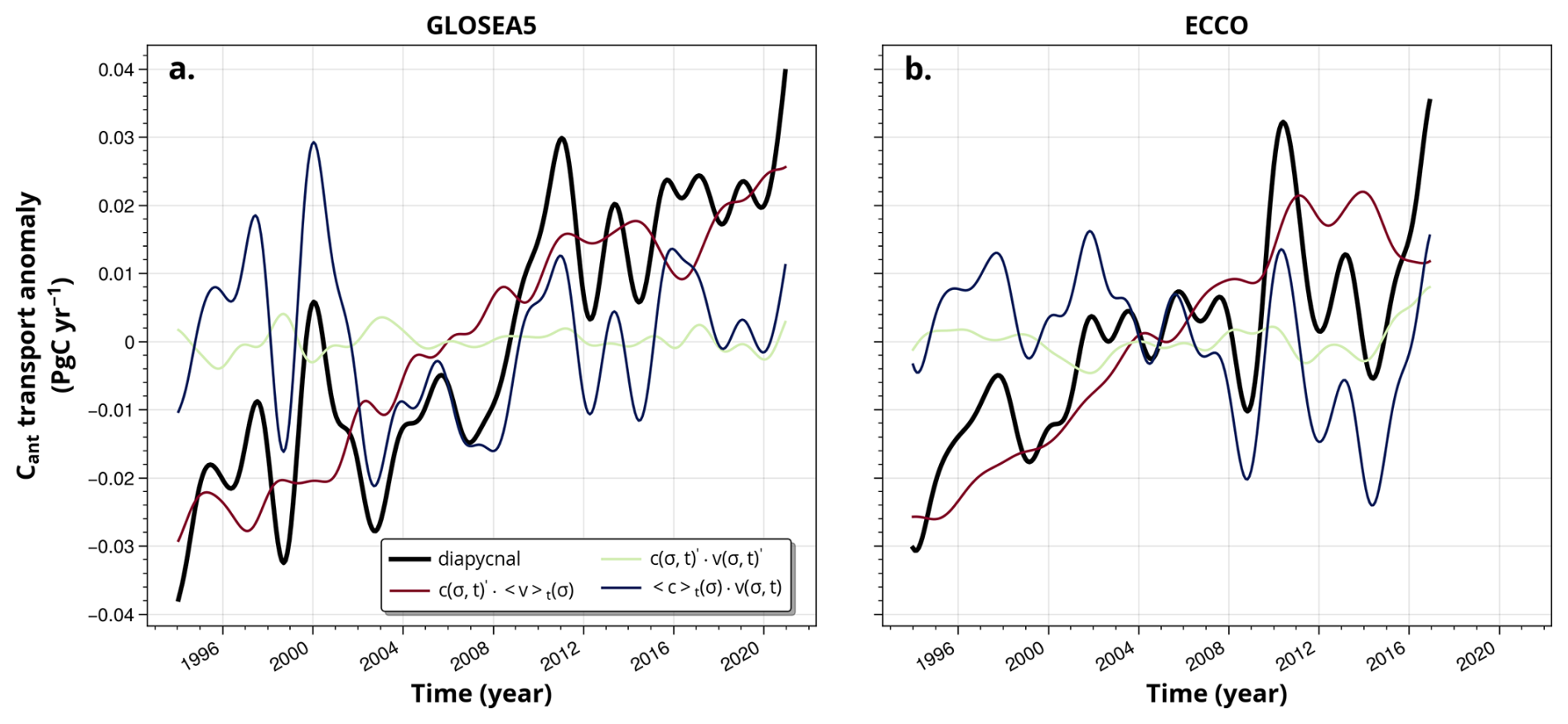
Figure 10 (a, b) Low-pass filtered signal anomaly of the diapycnal component of the net anthropogenic carbon (C_ant) transport along with its decomposition into a mean over time profile ($<c{>}_t\left(\mathit{\sigma }\right)$, $<v{>}_t\left(\mathit{\sigma }\right)$) and a perturbation ($c(\mathit{\sigma },t{)}^{\prime }$, $v(\mathit{\sigma },t{)}^{\prime }$) for the velocity and concentration terms in Eq. (3), for (a) GLOSEA5 and (b) ECCO.

4 Discussion

4.1 Time series evaluation

The [C_ant] derived from ocean reanalysis temperature and salinity, using NNs and the BC $\mathit{\phi }{C}_{\mathrm{T}}^{\mathrm{0}}$ approach, collectively referred to here as the OR-NN-BC method, shows good agreement with the 2002–2018 cruise-based estimates presented here using the same BC approach (RMSD of 5.1 µmol kg⁻¹ Table S1 and Fig. 2b), and with previous estimates at A25 reported by Zunino et al. (2014). The agreement between reanalysis products and bottle data was evaluated and summarized in Tables 4, S3, S5, and discussed in Sect. 2.8.2 and 2.8.3. The [C_ant] increase rates obtained from our [C_ant] time series are also in good agreement with the cruise-based rates. Here, we found [C_ant] increase rates of 0.7 ± 0.03, 0.2 ± 0.006 and 0.3 ± 0.004 µmol kg⁻¹ yr⁻¹ for the uMOC, lMOC and the section average, respectively, during the entire period (1993–2022) (Fig. 2b). These results closely match the [C_ant] increase rate estimates by Zunino et al. (2014) of 0.6 ± 0.3, 0.2 ± 0.3 and 0.3 ± 0.2 µmol kg⁻¹ yr⁻¹ for the same layers, based on A25 cruise data spanning 1997–2010. The agreement between both estimates, considering the two distinct periods used for the calculations, highlights the linear nature of the [C_ant] increase over time for all the layers under consideration. Looking at specific longitudinal regions of the A25 section, the [C_ant] increase rate in the IS (0.36 ± 0.005 µmol kg⁻¹ yr⁻¹) is slightly higher than the increase rate for the section average (Fig. S3i, j), likely due to the transfer of [C_ant] to intermediate depths in the IS by deep convection (Pérez et al., 2018; Asselot et al., 2024). This increase rate is comparable to that observed in the North East Atlantic Deep Water in the Labrador Sea (0.3 µmol kg⁻¹ yr⁻¹ for 1986–2016), but substantially lower than the 0.8 µmol kg⁻¹ yr⁻¹ rate found in Labrador Sea Water over the same period (Raimondi et al., 2021). This difference reflects the enhanced [C_ant] storage capacity of Labrador Sea compared to that of the IS, which results from its direct exposure to frequent deep convection events that efficiently transport [C_ant] from the surface to depths up to 2000 m (Raimondi et al., 2021; Yashayaev, 2024).

A comparison of C_ant transports with previous studies at A25 also reveals good consistency of the results. The cruise-based estimate of 0.092 ± 0.010 PgC yr⁻¹ by Pérez et al. (2013) for June 2004 is similar to our estimate of 0.09 ± 0.02 PgC yr⁻¹ for the same period (Fig. 7c). The 2002–2010 C_ant transport of 0.096 ± 0.011 PgC yr⁻¹ (254 ± 29 kmol s⁻¹) reported by Zunino et al. (2014) is comparable to the 0.098 ± 0.02 PgC yr⁻¹ that we find for the same period. Our [C_nat] estimates are also in good agreement with the 2002–2018 cruise-based [C_nat] values (Table S3), showing no long-term trend. The C_nat transport estimates derived from ocean reanalysis (net, uMOC and lMOC) are generally consistent with the A25 cruise-based estimates presented in this study, lying within their uncertainty range (Fig. 6, Table S7), except in 2006, when the discrepancy between the two values exceeded the uncertainty (Fig. 6a, c). Taking into account what happens on an intraannual scale, the seasonality of ML [C_nat] and the seasonality of surface [C_nat] and [DIC] (Figs. 4a, S6) are consistent with seasonal amplitudes in the range of 42–60 µmol kg⁻¹ observed for surface [DIC] at high latitudes (Keppler et al., 2020; Hagens and Middelburg, 2016) and ≈ 60 µmol kg⁻¹ for surface [DIC] in the SPNA (Leseurre et al., 2020; Reverdin et al., 2018). Finally, we note the lack of previous research on the seasonality of C_ant and C_nat transports in the SPNA.

This study corroborates previous estimates (Zunino et al., 2015; Pérez et al., 2013), which relied on cruise observations, and provides a more detailed perspective on C_ant and C_nat concentration and transport variability at seasonal to interannual time scales.

4.2 Mechanisms involved in seasonality

The deepening of the ML in winter favors the enrichment of [C_nat] within the ML through the entrainment of DIC-rich thermocline waters (Keppler et al., 2020; Takahashi et al., 1993), increasing the seawater partial pressure of CO₂ (pCO₂) and thus leading to surface saturation or slight supersaturation. In this study, we quantify that this physical mechanism of the mixed-layer pump accounts for approximately two-thirds of the winter increase in ML [C_nat] (Fig. 3). ML [C_nat] decreases in summer. During this period, changes in the depth of ML account for only one-third of the ML [C_nat] variability, with the remaining two-thirds largely favored by extensive biological carbon consumption (Keppler et al., 2020) resulting in surface undersaturation (Olsen et al., 2008; Lacour et al., 2015; Tjiputra et al., 2012).

It is important to note that the OR-NN-BC method relies solely on T, S, date, and position as predictor variables to obtain [DIC] from which the [C_nat] and [C_ant] components are derived (see Sect. 2.4). Hence, by methodology, we expect that the surface [C_nat] and [C_ant] correlate or anti-correlate to a certain extent with temperature (Figs. S7, S8). However, this does not imply that the temperature itself (i.e. solubility) is the sole or dominant driving mechanism of the observed seasonal surface [C_nat] and [C_ant] variability. For [C_nat], the seasonal cycle, which anti-correlates with temperature (Fig. S7a, b), still remains when considering no seasonal temperature signal at all (Fig. S7c, d). For [C_ant], however, there is a positive correlation with temperature (Fig. S8), and when the seasonal cycle of temperature is removed (Fig. S8c, d), the [C_ant] seasonal signal largely disappears. This effect reflects seasonal changes in the ocean's CO₂ uptake capacity rather than temperature-driven solubility control: summer conditions show minimum Revelle factor values (Fig. S4), which indicates enhanced seawater buffer capacity, thereby favoring [C_ant] uptake. Together, summer changes in both [C_nat] and [C_ant] components are indicative of an enhanced uptake of atmospheric CO₂ in the SPNA (Rodgers et al., 2023; Rustogi et al., 2023).

At the intraaanual scale, C_nat and C_ant transports are dominated by seasonal variations in volume transport, driven by uMOC volume changes in the EGC and velocity variations in the eastern boundary current (Mercier et al., 2024). At A25, this combined effect of uMOC thickness variations and velocity changes on seasonal tracer transport variability differs from C_ant transport variability at 26.5° N in the subtropical gyre, which was attributed primarily to velocity variability (Brown et al., 2021) (Fig. S9). Less seasonal variation in C_ant transport is observed in the SPNA at the A25 section (amplitude of 0.015 PgC yr⁻¹) (Fig. 7e–f)) than at 26.5° N (peak-to-trough amplitude of 0.08 PgC yr⁻¹) (Brown et al., 2021). However, the large seasonal variations for uMOC and lMOC represent more than 25 % of the annual average for volume and tracer transports at A25. Likewise, at 26.5° N between 2004 and 2012, the seasonal variability in the transport of uMOC C_ant constituted 27 % of its mean value (Brown et al., 2021).

4.3 Interannual to long-term mechanisms

The long-term [C_ant] increase at A25 is linear (Fig. 8). This rise is primarily driven by the atmospheric increase in CO₂ and the increase in air-sea CO₂ fluxes in the NA (Gruber et al., 2023), as suggested by the trend-less C_ant transport at 26.5° N between 2004 and 2012 (Brown et al., 2021). The decadal rate of increase in [C_ant] in the water column depends on the distance of the layer from the sea surface, with higher increase rates closer to the surface where atmospheric [C_ant] enters the ocean via air-sea exchange (Fig. 5). For example, a rate of increase of 6.0 µmol kg⁻¹ per decade was found for the uMOC compared to 2.4 µmol kg⁻¹ per decade for the lMOC. However, the relative increase for each layer is the same. The atmospheric CO₂ growth was about 61.35 ppm for 1993–2022 (1993: 357.21 ppm, 2022: 418.56 ppm) (Lan et al., 2023). This rise resulted in an almost doubling of [C_ant] in ML (49.8 %). [C_ant] variability is dominated by long-term changes in concentration, due to atmospheric CO₂ forcing, while [C_nat] variability is dominated by seasonal and interannual changes.

The interannual variability in ML [C_nat] and [C_ant] is the strongest when particularly deep ML are found during deep convection periods, before 1995 (for [C_nat]) and between 2008–2016 (for both) (Figs. 5, S3). The interannual variability of seasonal deep convection events shapes the interannual [C_nat] and [C_ant] in the ML. The signal is the largest in the IS and in agreement with previously reported events (Piron et al., 2016, 2017). In turn, the alternation of shallow and deep ML and the persistence of the signal at depth cause interannual variability in concentrations.

At 24.5° N, the rates of increase in [C_ant] between 0.25 and 0.88 µmol kg⁻¹ yr⁻¹ were observed between 1992 and 2011 for deep waters and surface layers, respectively (Guallart et al., 2015). This is consistent with our increase rate for 1993–2011 of 0.2 µmol kg⁻¹ yr⁻¹ for deep waters and more than 0.8 µmol kg⁻¹ yr⁻¹ in ML. Motivated by the study of Müller et al. (2023) on GLODAP data spanning over 1994 (1989–1999), 2004 (2000–2009) and 2014 (2010–2020) decades, we computed the accumulation rates obtained with our method for these three decades at A25 (the first decade for us is limited and starts in 1993). Despite using a different methodology, we observe the reduction in [C_ant] accumulation rate in the North Atlantic (Steinfeldt et al., 2024) at A25, with a lower [C_ant] increase rate above 3000 m in the 2014 decade (3.4 µmol kg⁻¹ per decade) than in the 1994 and 2004 decades (4.0 µmol kg⁻¹ per decade) (Fig. 11). This reduction is concomitant with the observation of deeper ML at the end of the 2011–2020 period (Fig. S2). The maximum [C_ant] reduction is located on the Reykjanes Ridge (Fig. 11b), suggesting that the NAC brought less [C_ant] during the 2014 decade. The early 1994 decade and the 2014 decade correspond to periods when the subpolar gyre was more intense and less affected by NAC waters (Häkkinen and Rhines, 2004; Marzocchi et al., 2015; Zunino et al., 2020; Holliday et al., 2020). In addition, deeper ML (as in the 2014 decade) would lead to a minimum in [C_ant], even if the [C_ant] from the NAC was higher or unchanged.

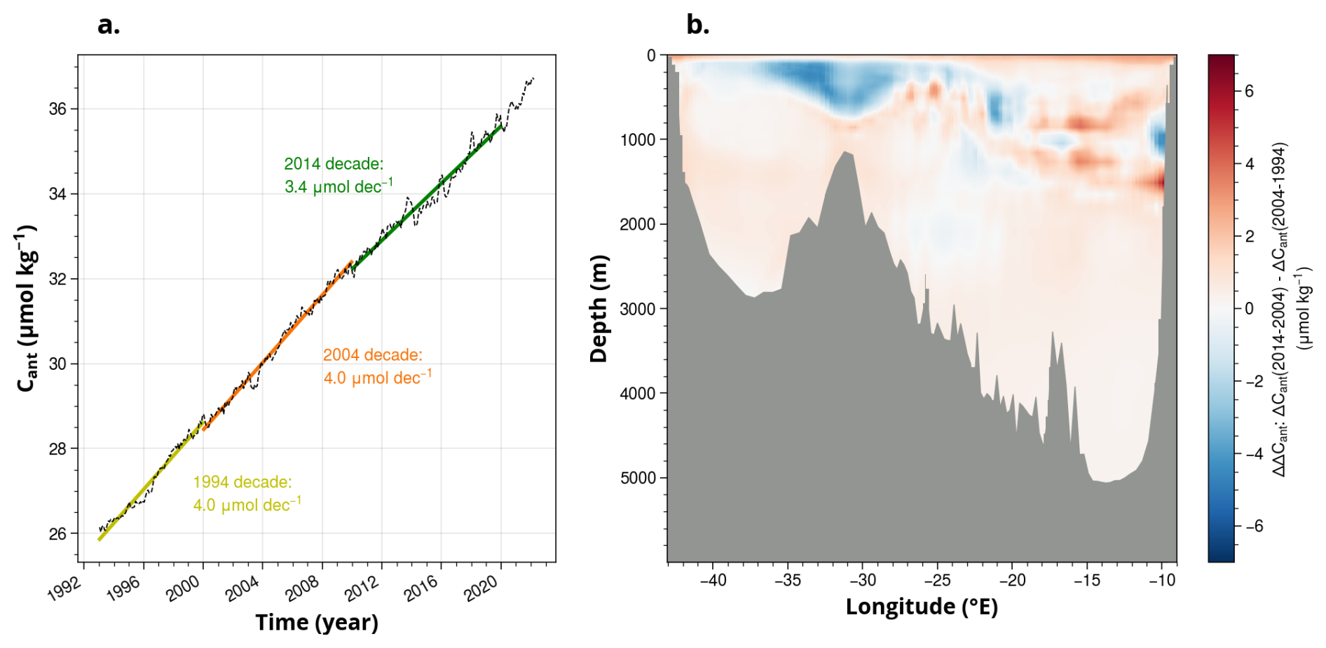
Figure 11 (a) C_ant increase rate for the 0–3000 m depth range according to the estimates calculated from GLOSEA5 reanalysis. The decades are centered like in Müller et al. (2023). (b) ΔΔC_ant: difference in increase rate between 2014–2004 and 2004–1994 decades at A25 section.

Looking at volume transport, an interannual decrease is observed in the net and MOC transports until the early 2010s as in Jackson et al. (2022) (Fig. 8a) and is consistent with the weakest state of the AMOC in recent decades (Caesar et al., 2018, 2021; Boers, 2021; Jackson et al., 2022; Mercier et al., 2024) before increasing since then (Fig. 8a).

For C_ant transport, the decadal time scale that shows a linear trend is not driven by circulation but by the linear growth in [C_ant], compared to C_nat, a result that refines previous results, obtained over a shorter time frame in the subtropical and subpolar gyres, which concluded that the variability of C_ant transport is driven by circulation (Brown et al., 2021; Pérez et al., 2013). Most of the net C_ant transport variability comes from its diapycnal component, which is set by [C_ant] growth (Figs. 9, 10). There is a significant imbalance between the C_ant transports of the uMOC and the lMOC due to the [C_ant] strong vertical gradient so that the uMOC is the main driver of the North Atlantic northward transport of C_ant (Brown et al., 2021; Pérez et al., 2013). The increase in [C_ant] results in almost a doubling of the northward C_ant transport from 0.08 PgC yr⁻¹ in 1992 to 0.15 PgC yr⁻¹ in 2022. Over the shorter pre-2008 period, C_ant transport exhibited a slower increase rate (0.013 PgC per decade compared to 0.038 PgC per decade after 2008), attributed to weakened MOC strength (uMOC decreased by 1.8 Sv per decade before 2008) that attenuated the increase in [C_ant].

The variability of the C_nat net transport is driven by the variability of volume transport from intraannual to long-term scales, in agreement with Zunino et al. (2014, 2015), and that [C_nat] is mainly constant throughout the time range of this study. Relative changes in mean [C_nat] are small (Fig. 2), so long-term C_nat transport changes are mainly determined by volume transport changes. Since C_nat transport strongly correlates with net volume transport in the subpolar gyre, having the latter well constrained and solved is crucial. The interannual net C_ant transport variability is also circulation-driven because relative changes in [C_ant] are not significant in successive years contrary to the relative changes in volume transport. The net volume transport of GLOSEA5 increases while ECCO one stays constant, which is reflected as well on net C_nat transports. The transport of uMOC C_nat also shows the periods of reduction and strengthening before and after 2008–2012, and is based on the diversity in the physics of ocean reanalysis. Due to the strong volume transport-driven variability of net C_nat transport, the spread of circulation in ECCO and GLOSEA5 has a greater influence on net C_nat decadal transport than on decadal net C_ant decadal transport, being more influenced by [C_ant] (see Sect. 2.8.3 and Tables 4, S5 for a comparison of ocean analysis products).

4.4 NA C_ant budget implications

The C_ant budget of an oceanic region is the result of the balance between lateral advection, air-sea fluxes, and storage. Net advective transport plays an important role in the NA budget, contributing to 65 ± 13 % of the NA C_ant storage rate (reference to 2004, Pérez et al., 2013). The observed increase in net northward C_ant transport over the 30-year period is evident in both subtropical and subpolar regions of the NA, as documented through decadal GO-SHIP section repeats (Caínzos et al., 2022). At A03, C_ant transport experienced an increase from 0.058 ± 0.036 to 0.104 ± 0.035 PgC yr⁻¹ between 2000–2009 and 2010–2019, while at 26.5° N C_ant transport passed from 0.128 ± 0.032 to 0.222 ± 0.024 PgC yr⁻¹ (Caínzos et al., 2022) (Fig. S9). During the same time periods (2000–2009 and 2010–2019), we found at A25 an increase in northward C_ant transport from 0.09 ± 0.02 PgC yr⁻¹ to 0.11 ± 0.03 PgC yr⁻¹. At AR07, north of A25, similar values as at A25 are found: 0.088 ± 0.038 for 2000-2009 and 0.115 ± 0.042 PgC yr⁻¹ for 2010–2019 (Caínzos et al., 2022) (Fig. S9). The 73 %–79 % increase in C_ant transport in the subtropical region between 2000–2009 and 2010–2019 is greater than the 22 %–32 % increase in the subpolar region. However, stable C_ant transport is found at 26.5° N over a shorter period (2004–2012) at high resolution (Brown et al., 2021), suggesting an analysis over a longer period to better identify long-term trends and a better consensus between distinct methods. The 2004–2012 average C_ant transport convergence between A25 and 26.5° N is equal to 0.091 ± 0.033 PgC yr⁻¹: 0.191 ± 0.013 PgC yr⁻¹ at 26.5° N (Brown et al., 2021) minus 0.10 ± 0.02 PgC yr⁻¹ at A25. Therefore, the northward transport of C_ant at A25 is half the one observed at 26.5° N, similar to previous findings (Pérez et al., 2013). Due to the northward increase in C_ant transport at A25 concomitant with its constant supply at 26.5° N, the convergence is greater (reduced) at the beginning (end) of the time period. We found that the lateral C_ant transport convergence between A25 and 26.5° N averages to 0.13 ± 0.07 PgC yr⁻¹ in 2004 and 0.10 ± 0.05 PgC yr⁻¹ in 2012. The documented increase in air-sea CO₂ fluxes between A25 and 26.5° N during this period (Gruber et al., 2023) may partially offset this reduced convergence; however, this compensation would imply a decrease in storage.

4.5 Limits of the OR-NN-BC method

This study represents the first quantitative assessment of [C_ant] seasonality in the SPNA, and no comparable studies exist in the literature to validate or challenge these findings. The seasonality of [C_ant] may depend on the approach used to calculate it, and further investigations based on other [C_ant] estimation approaches (TTD, TrOCA, $C_{\mathrm{IPSL}}^{\mathrm{o}}$, ΔC^*) may be of interest. The abiotic model, used as an assumption in the BC approach to determine the saturation of [C_ant] in the first 25 m based solely on the fraction of atmospheric CO₂, is a good approximation to constrain [C_ant] seasonality at the sea surface. We obtained a seasonal variation of ML [C_ant] of ±2.5–3.0 µmol kg⁻¹, that is 1.1 µmol kg⁻¹ higher (on average) compared to seasonal [C_ant] in ML for an annual [C_ant] profile (difference between ML and ML annual in Fig. 3d). The natural variability of [DIC] coming from NN is an order of magnitude higher (Fig. 3b, d). We found a ±12.5 µmol kg⁻¹ amplitude increase on average in ML [C_nat] compared to ML [C_nat] applied to annual [C_nat] profile (Fig. 3b). The natural variation of the CO₂ fraction in surface water, motivated by natural processes, and here incorporated in the OR-NN-BC method owing to NN, is then an order of magnitude higher than the variability caused by the increase in the anthropogenic fraction of CO₂ in the atmosphere.

Our results show that the seasonal variability of ML [C_nat] and C_ant is generally well captured by surface C_nat and C_ant concentrations (Fig. S10), as the difference between surface and ML mean concentrations remains nearly constant throughout most of the year (within −8.6 ± 4.9 µmol kg⁻¹ for [C_nat], and 1.8 ± 0.4 µmol kg⁻¹ for C_ant). Surface concentrations therefore provide a reasonable proxy for seasonal variability within the ML, except in winter. In March, deviations in [C_nat] ([C_ant]) of up to 16.8 (2.7) µmol kg⁻¹ are observed between surface and ML values. These differences result from the combined effect of a slight vertical decrease (increase) in [C_ant] ([C_nat]) within the winter ML, and a deeper winter ML in the IS relative to the rest of the section (Fig. S3). The non-uniformity of ML [C_ant] for winter deep ML has also been reported using a similar methodology with Argo-O₂ profilers in the IS (Asselot et al., 2024). In our case, this effect is further amplified by the NN-generated [O₂], which exhibits a vertical gradient within the ML. This pattern likely reflects a methodological artifact rather than a physical signal, as Argo-O₂ observations generally show a vertically homogeneous [O₂] distribution within the winter ML in the IS (Piron et al., 2016, 2017; Wolf et al., 2018). Consequently, the NN-induced [O₂] vertical gradient amplifies the vertical gradients in ML [C_ant] and [C_nat], and such methodological limitation should be taken into account when applying the OR-NN-BC method.

As for the inter-product comparison, GLOSEA5 simulates deeper ML values in winter and shallower ML in summer than ECCO (Fig. S2), producing higher (lower) ML [C_nat] values in winter (summer), thereby amplifying the seasonal carbon signal. In contrast, the weaker ECCO ML depth seasonal amplitude dampens the seasonal variability of this property. The opposite behavior is observed for [C_ant] owing to its opposed vertical gradient.

When looking at the interannual-to-long-term signal, this study suggests that the results in C_ant increase rates depend strongly on the period chosen. Interannual variability is added to the linear trend, giving different results depending on the chosen period. Continuing to address [C_ant] variability at higher resolution on multiple time scales is also of interest.

To summarize, and despite the methodological limitations discussed in this section, we are confident in our results regarding the main interannual variability signals and long-term trends in concentrations and transport, as well as for the mean seasonal cycle of [C_nat], which are supported by other independent studies. For [C_ant], however, this study represents the first quantitative assessment of [C_ant] seasonality in the SPNA, and no comparable studies exist in the literature to validate or challenge these findings. Each reanalysis shows good agreement with A25. However, year-round hydrographic data is not available for comparison with the seasonal transport estimates from the reanalysis. This would be all the more interesting in winter, when seasonal maxima for most of the concentrations and transports presented in this study are observed. In addition, the study of specific high-frequency processes will require additional data sources to further discuss the results and explore each of the reanalysis rather than an average signal. Finally, our results will depend even more on the reanalysis chosen if volume transport is predominant in the process, i.e. for [C_nat] transport (seasonal and interannual) and seasonal [C_ant] transport.

5 Conclusions

This study establishes the first nearly 30-year time series of natural (C_nat) and anthropogenic (C_ant) carbon properties and transports in the SPNA at the A25 section. The novelty of this study lies in the combination of neural networks (NN) and ocean reanalysis temperature and salinity fields to estimate C_nat and C_ant (with errors), yielding monthly-resolution results consistent with biennial summer observations. The resulting time series enable the analysis of variability across time scales, from seasonal to interannual and long-term, relative to hydrographic sections.

Large seasonal variability was evidenced in the mixed layer (ML) and the upper branch of the meridional overturning circulation (uMOC), the ML showing the strongest seasonal variations in tracer concentrations. For C_nat concentrations, seasonal variability dominates over interannual and long-term signals. We found that winter ML deepening (here referred to as mixed layer pump) accounts for two-thirds of the ML C_nat seasonal cycle. In summer, however, the changes in ML depth explain only one-third of the ML C_nat seasonal cycle, with the remainder mainly attributed to biological activity, which peaks at this time of year. In contrast, for C_ant concentrations, the long-term signal dominates over seasonal and interannual variability. The long-term increase averages to 0.3 ± 0.004 µmol kg⁻¹ yr⁻¹ for the entire section and reaches 0.825 ± 0.016 µmol kg⁻¹ yr⁻¹ in the ML. Despite the relatively small seasonal amplitude of C_ant concentrations, ML C_ant also exhibited intraannual variability. In this case, the mixed layer pump accounted for about one-quarter of the mean ML C_ant variation in summer and half of the seasonal signal in winter, the remainder likely linked to seasonal changes in the Revelle factor.

In terms of lateral tracer transport, we observed seasonal peak-to-peak amplitudes of about 25 % of the annual average for the uMOC (lMOC). Therefore, significant differences in C_nat and C_ant uMOC transports can arise when comparing annual to synoptic data. Since observations of the A25 OVIDE cruise are summer dependent, further reference observations in winter might be a key element in better constraining the seasonal cycles of carbon and corresponding transport.

The variability of tracer transport is largely governed by volume transport for both C_nat and C_ant on all evaluated time scales, except long-term C_ant transport, which is driven by changes in [C_ant] – ultimately linked to rising atmospheric CO₂ concentrations. We show the rapid increase in [C_ant] at different rates in the water column and how it influences northward C_ant transport. In general, the uniform vertical relative increase in [C_ant] combined with steep vertical gradients creates a disequilibrium in meridional [C_ant] transport, and this imbalance intensifies as atmospheric concentrations continue to rise. We speculate that the projected reduced AMOC, which may already have begun (e.g. Caesar et al., 2018), will reinforce the [C_ant] gradient between the upper and lower limbs of the MOC as the accumulation of [C_ant] at depth will be less rapid and [C_ant] will continue to grow.

Regarding interannual variability, the most pronounced anomaly in volume transport occurred around 2010, also affecting tracer transport due to circulation-driven variability. A significant C_ant transport anomaly in 2010, previously documented at 26.5° N, was attributed to a decrease in volume transport during that year. Here we found that a persistent long-term decrease in the uMOC volume transport was observed up to 2010. The two ocean reanalysis used to evaluate net transports (GLOSEA5 and ECCO) presented similar values before 2010, supporting the reliability of this anomaly, but diverged afterwards, leading to larger discrepancies in the tracer transport post 2010. This discrepancy in the datasets is not attributable to an inherent signal but rather to the methodologies employed in the construction of the reanalyses. The period of reanalysis divergence aligns with the freshening of the eastern subpolar gyre that began in the late 2010s and peaked in 2016 (Fox et al., 2022). Together, these observations and our results indicate a transition period around 2010 with impacts on the carbon dynamics.

This study, based on ocean reanalysis, connects with studies using high-resolution Argo-O₂ Lagrangian profilers to analyze biogeochemical properties (Asselot et al., 2024) and helps to resolve natural and anthropogenic oceanic carbon cycles, providing results that can contribute to the evaluation of the impacts of climate change on marine ecosystems amid uncertain ocean responses (Henson et al., 2022). Expanding the BGC-Argo float network (including Argo-O₂ profilers), combined with NN and multiple linear regression (MLR) techniques (Keppler et al., 2020; Müller et al., 2023; Brown et al., 2021), will improve understanding of biogeochemical cycles and parameterization of biogeochemical processes in Earth system models. NN and MLR techniques are effective in filling data gaps, but perform poorly in data-scarce regions due to limited training. Ultimately, enhancing the spatio-temporal coverage of ocean observations will refine climate projections and assessments of ocean carbon storage. Increasing data from BGC-Argo will also support NN training to capture diverse oceanic states under climate change, particularly for carbon dynamics and acidification (Pérez et al., 2013; Gruber et al., 2023). GLODAP's extensive North Atlantic coverage (Olsen et al., 2019) aids in reliable reference data for NN training, ensuring minimal errors. Although in this study we did not find that the use of O₂ as input to NN improved the estimation of layer-averaged variables, O₂ plays a central role in biological processes such as photosynthesis/remineralization. Thereby, including O₂ data, for example, through Argo-O₂ profilers, will reduce errors in the estimation of carbon variables in discrete locations, especially close to the sea surface (Bittig et al., 2018; Carter et al., 2021; Asselot et al., 2024).

A logical next step following the present study would be to apply the method used here to 4D gridded fields to quantify [C_ant] between several ocean sections and to identify the connections between advection and inventory changes in C_ant in different ocean regions. Properly accounting for uncertainty in the C_ant inventory opens up many possibilities for future work aimed at better understanding the processes governing ocean's anthropogenic and natural carbon budgets.