Land surface model underperformance tied to specific meteorological conditions

The exchange of carbon, water, and energy fluxes between the land and the atmosphere plays a vital role in shaping global change and extreme events. Yet our understanding of the theory of this surface-atmosphere exchange, represented via land surface models (LSMs), continues to be limited, highlighted by marked biases in model-data benchmarking exercises. Here, we leveraged the PLUMBER2 dataset of observations and model simulations of terrestrial sensible heat, latent heat, and net ecosystem exchange fluxes from 153 international eddy-covariance sites to identify the meteorological conditions under which land surface models are performing worse than independent benchmark expectations. By defining performance relative to three sophisticated out-of-sample empirical models, we generated a lower bound of performance in turbulent flux prediction that can be achieved with the input information available to the land surface models during testing at flux tower sites. We found that land surface model performance relative to empirical models is worse at edge conditions – that is, LSMs underperform in timesteps where the meteorological conditions consist of coinciding relative extreme values. Conversely, LSMs perform much better under “typical” conditions within the centre of the meteorological variable distributions. Constraining analysis to exclude the edge conditions results in the LSMs outperforming strong empirical benchmarks. Encouragingly, we show that refinement of the performance of land surface models in these edge conditions, consisting of only 12 %–31 % of all site-timesteps, would see large improvements (22 %–114 %) in an aggregated performance metric. Better performance in the edge conditions could see mean relative improvements in the aggregated metric of 77 % for the latent heat flux, 48 % for the sensible heat flux, and 36 % for the net ecosystem exchange on average across all LSMs and sites. Precise targeting of model development towards these meteorological edge conditions offers a fruitful avenue to focus model development, ensuring future improvements have the greatest impact.

1 Introduction

Our ability to predict future climate and its impact on the places where we live largely rests on our ability to model the land surface (Charney, 1975; Friedlingstein et al., 2014, 2025; Arora et al., 2020; Canadell et al., 2021). Turbulent fluxes of carbon, water, and energy link terrestrial processes with atmospheric dynamics and oceanic freshwater input. As the climate changes, these land-atmosphere interactions will be altered as the behaviour of both the land surface and the atmosphere is impacted (Cao et al., 2021; Walker et al., 2021). As such, it is necessary that our knowledge of terrestrial processes is robust and well-developed.

Land Surface Models (LSMs) simulate the surface carbon, water, and energy cycles and their interaction with the boundary layer (the lowest part of the atmosphere directly influenced by the land surface) and are important components of Earth System Models (ESMs) that are used to create future climate projections. Since LSMs integrate our current knowledge of terrestrial processes, they are an ideal testbed for evaluating the extent and efficacy of our understanding. While all LSMs are based on fundamental theory and physical processes, implementations can vary substantially whether via equations, parametrisation, approach to approximations, or the number of processes represented, with multiple independent modelling teams producing their own unique LSMs (Fisher and Koven, 2020). In turn, the outputs from LSMs can also exhibit significant differences, resulting in a wide range of contemporary simulations and future projections of the terrestrial carbon, water, and energy cycles (Arora et al., 2020).

Analysing LSM performance can provide important feedback on our understanding of terrestrial processes. Analysis conducted against observations yield estimates of accuracy (Blyth et al., 2011). Comparing LSMs against each other, either in coupled simulations as part of ESMs as seen within progressive phases of the Coupled Model Intercomparison Projects (CMIP, Eyring et al., 2016) such as CMIP6 (Gier et al., 2024), stand-alone implementations such as the PILPS (Henderson-Sellers et al., 1996) and TRENDY projects (Sitch et al., 2015, 2024), or even the combination of coupled and offline simulations (e.g. LS3MIP, van den Hurk et al., 2016), provides a measure of model uncertainty that can advance our understanding of terrestrial processes. A relatively novel approach to LSM evaluation is that of benchmarking LSMs against a priori expectations of performance as used in the PLUMBER framework (Best et al., 2015; Haughton et al., 2018b). Model intercomparisons alone rarely guide model refinement as quantifying intermodel spread or demonstrating that one model is marginally superior does not provide insight into the processes or input conditions causing such performance discrepancies. Here we used data from the PLUMBER2 benchmarking experiment to answer three questions that might more constructively contribute to LSM development:

1. Under what specific meteorological input conditions does each land surface model consistently underperform in simulations of net ecosystem exchange, latent heat, and sensible heat fluxes?

2. Are the conditions where each LSM underperforms similar across different LSMs and fluxes?

3. How much do these conditions, and the subsequent underperformance when simulating fluxes, influence the overall performance of LSMs in benchmarking studies, such as PLUMBER2?

To answer the first question, it is necessary to define “underperformance”. To do so, we turn to the PLUMBER benchmarking framework and its second iteration, PLUMBER2 (Best et al., 2015; Abramowitz et al., 2024). PLUMBER2 includes multiple LSM simulations using harmonised input data from a set of eddy-covariance sites (Ukkola et al., 2022). In addition, it includes a series of out-of-sample empirical flux models (EFMs) which also simulate the fluxes at the same sites to provide performance measures independent of the LSMs. By comparing LSM outputs to those of EFMs of increasing complexity, PLUMBER2 creates a range of potential performance expectations predicated on the information available to the LSMs – the EFMs provide lower bounds of flux prediction skill based on the input data (Haughton et al., 2018a) – and LSMs can then be assessed on their accuracy relative to these benchmarks (Abramowitz et al., 2024). As such, here we define “underperformance” as instances where the LSM does not achieve these empirically-derived lower bounds of predictive skill.

Next we must consider what is meant by “conditions”. The PLUMBER2 dataset includes a wide variety of eddy-covariance sites – over 150 eddy-covariance sites situated in more than 20 countries and comprising of 11 vegetation classes (Ukkola et al., 2022). While this is a biased sampling of the global land surface (Alton, 2020; Chu et al., 2017, 2021; Griebel et al., 2020), the dataset does capture a broad range of ecosystems, climate regimes and weather conditions (van der Horst et al., 2019; Beringer et al., 2022). Therefore, the PLUMBER2 domain space is likely to be suitable for assessing LSM performance and identifying specific conditions where LSMs underperform. Identifying “poor performance” conditions based on plant functional type (PFT) classifications or individual site behaviour is unlikely to provide clear directions for improvement (Haughton et al., 2018a). PFTs are poor descriptors of flux-meteorology interactions, so grouping sites in this manner is likely to obscure the cause of performance issues (Cranko Page et al., 2024). Similarly, studies have repeatedly analysed LSM performance during meteorological conditions defined at longer timescales – such as the monthly scales used in the TRENDY project (Sitch et al., 2024) – with conditions such as droughts being poorly modelled by LSMs (Bastos et al., 2021; De Kauwe et al., 2015; Gu et al., 2016). However, most LSMs operate with approximately half-hourly timesteps meaning that any emergent biases ultimately originate from biases at this timescale, and so in this study, we consider meteorological conditions at this higher temporal resolution. Analysis at half-hourly resolution is unlikely to adversely penalise LSMs (Haughton et al., 2016) but could provide crucial information on conditions in which LSMs underperform and the processes responsible, including issues of process representation associated with diurnal cycles, fast processes such stomata functioning, or particular transient weather conditions (e.g. clouds).

To answer whether all LSMs reliably underperform in similar conditions we can again lean on the PLUMBER benchmarking framework. Multiple LSMs were run with the same information at the same eddy-covariance sites, facilitating comparison between LSMs in a robust manner (Abramowitz et al., 2024). If all LSMs routinely underperform in the same half-hourly meteorological conditions, this would imply there are processes at play that are either consistently missing or incorrectly represented across all models. However, if the conditions under which each LSM underperforms differ, then information on correct process representation and parametrisation might be derived from these differences.

When considering LSM performance, the initial PLUMBER2 analysis found that LSMs perform poorly against benchmarking EFMs (Abramowitz et al., 2024). In fact, LSM simulations of turbulent fluxes were often of worse quality than those from simple empirical models when the modelled fluxes were compared via an aggregated measure of seven independent performance metrics. This result may derive from a base level of LSM underperformance under all meteorological conditions – the LSMs may just consistently be slightly worse than the EFMs. However, potentially, this poor LSM performance against EFMs could be caused by the specific conditions in which LSMs underperform. If this is the case, we could identify the region of input space of meteorological conditions that is responsible for the poor LSM performance relative to the benchmarks in PLUMBER2 and help constrain areas for future model development.

We might hypothesise that the conditions of worst EFM performance will be in those areas where the EFMs may be lacking training data. Such conditions will be associated with meteorological extremes, which due to their nature are observed less frequently. Meanwhile, the EFMs should perform very well under “average” conditions – those meteorological conditions experienced the most across the available training data. As such, we hypothesise that the LSMs may underperform generally across the more temperate and hence “populated” meteorological conditions due to the better EFM performance under these conditions. However, since most LSM parametrisation is based on typical or good conditions conducive to normal ecosystem functioning, two possible contrasting hypotheses are posited regarding the extreme meteorological conditions. Firstly, that the lack of training data is a greater penalty to the EFMs and so LSMs have good performance at meteorological extremes relative to the EFMs. The alternative hypothesis is that the LSMs' lack of parametrisation at extremes is a bigger disadvantage than the lack of training data for EFMs, and hence the LSMs underperform in the extreme conditions.

A final hypothesis is that, under conditions where the observations used are erroneous but consistently biased (for example, conditions where the eddy-covariance method is biased due to violated assumptions such as during low wind speeds), the LSMs will underperform compared to the EFMs. This is because the eddy-covariance data is compromised and therefore the LSMs, being process-based, cannot model the biased observations, while the EFMs have no such constraints and can learn the biased behaviour under such conditions.

2 Methods

2.1 Data

2.1.1 Eddy-covariance Data

As part of the PLUMBER2 benchmarking framework, this study utilised the PLUMBER2 eddy-covariance dataset of observations (Ukkola et al., 2022). Of the 170 available sites, 153 were used in this study, as 17 sites were found to exhibit problematic or missing precipitation data (Abramowitz et al., 2024). For each site, observed fluxes of sensible heat (Qh), latent heat (Qle), and net ecosystem exchange (NEE) were available at a half-hourly timestep. Note that the PLUMBER2 dataset includes energy balance-corrected versions for each of these fluxes but these were not used in this study since Abramowitz et al. (2024) showed that using the energy balance-corrected data did not improve the overall performance of the LSMs. Locally-observed meteorology including downwelling surface shortwave radiation (SWdown), downwelling surface longwave radiation (LWdown), air temperature (Tair), vapour pressure deficit (VPD), specific humidity (Qair), relative humidity (RH), precipitation (Precip), surface air pressure (PSurf), CO₂ concentration (CO2air), and wind speed (Wind) was used as inputs to the models. The leaf area index (LAI) provided for each site in the PLUMBER2 dataset was also utilised. This LAI timeseries was derived from one of two remote sensing products, with this study using the preferred timeseries as detailed in Ukkola et al. (2022). In total, over 16 million individual site-timesteps were available in the dataset. Throughout this study, the three fluxes were analysed separately.

2.1.2 Models

The PLUMBER2 benchmarking framework involved 33 models, including seven empirical flux models and 26 process-based models. The details are specified in Abramowitz et al. (2024). To confine this study and ensure models were comparable, we here focussed on the 11 process-based models that are “Land Surface Models” or LSMs – that is, those models that are designed to be used in coupled climate modelling simulations. The models meeting this requirement are detailed in Table 1. Simulated NEE fluxes were not available for CLM5, JULES_GL9, JULES_GL9_LAI, and MATSIRO. In addition, ORCHIDEE2 and ORCHIDEE3 were lacking model outputs for all three fluxes at two and four sites, respectively. Additionally, this study used five of the PLUMBER2 EFMs in two different groups – the “benchmark” EFMs and the “best” EFMs. The “benchmark EFMs” were used to illustrate the full range of EFM performance when using models of increasing complexity and data needs. As such, they can be used to benchmark LSM performance aligning with their use in PLUMBER2. These were:

• the “1lin” model, a simple linear regression of flux against SWdown.

• the “3km27” model that used k-means clustering plus regression on three meteorological variables, namely SWdown, Tair and RH. 27 clusters were used to theoretically allow clusters where each meteorological variable is “low”, “medium”, and “high”.

• the “LSTM” model, a long short-term memory model that was provided similar information to the LSMs, including static site parameters such as vegetation type and canopy height.

Kowalczyk et al. (2006)Wang et al. (2011)Haverd et al. (2013, 2016, 2018)Balsamo et al. (2009)Boussetta et al. (2013)Dutra et al. (2010)van den Hurk et al. (2000)Lawrence et al. (2019)Dunne et al. (2020)Shevliakova et al. (2024)Best et al. (2011)Clark et al. (2011)Best et al. (2011)Clark et al. (2011)MATSIRO6 Document Writing Team (2021)Niu et al. (2011)He et al. (2023)Krinner et al. (2005)Vuichard et al. (2019)

Table 1 Land Surface Models included in this study. “No NEE flux” here refers only to the necessary 30 min outputs required for this analysis – the model may produce NEE simulations at a larger timestep.

The “best EFMs” were, as the name suggests, the three EFMs that performed best according to the aggregated metrics for NEE, Qle, and Qh in the PLUMBER2 framework (Abramowitz et al., 2024). These EFMs were the most complex EFMs used in the framework and were:

• the “6km729lag” model, which used k-means clustering plus regression across 6 meteorological variables – SWdown, Tair, RH, Wind, Precip, and LWdown – as well as lagged Precip and Tair in the form of mean values over the prior 1–7, 8–30, and 31–90 d. Similar to the “3km27”, the number of clusters was chosen such that each meteorological variable could be “low”, “medium”, or “high”, resulting in 729 clusters.

• the “RF” model which used the Random Forest method with SWdown, LWdown, RH, Qair, surface air pressure (Psurf), Wind, CO₂ concentration (CO2air), VPD, and LAI as predictors.

• the “LSTM” model as above.

By using three EFMs to define the best EFM performance, we reduced the influence of individual model structure on our results while also limiting any instances of a single EFM performing anonymously well and affecting the assessment of LSM performance.

In all cases, the EFMs were run out-of-sample for each site. For all but the “LSTM” model, this involved training the models on the timesteps from all but a single site to then predict the remaining site out-of-sample. For the “LSTM” model, three randomly chosen sites were held back from each model and this was repeated until all sites had been simulated out-of-sample. As such, each EFM is the collective output from multiple models trained on all but one or three sites and then simulating the individual unseen sites. Similarly, for all but the “LSTM” model, each of the three fluxes used separate models. The “LSTM” model predicted NEE, Qle, and Qh in each model.

2.2 Analysis

2.2.1 Defining Poor LSM Performance

To analyse the conditions under which the LSMs could be expected to perform better, we compared LSM error to the errors of the best EFMs at each site-timestep. The absolute model error was calculated as:

$$\begin{array}{}\text{(1)}& {\displaystyle }{\displaystyle }{\text{Error}}_{\text{Mod}}\left(t\right)=\left|{\text{Flux}}_{\text{Mod}}\right(t)-{\text{Flux}}_{\text{Obs}}(t\left)\right|\end{array}$$

for each LSM and the three best EFMs (step 2 in Fig. 1). We then defined an individual timestep as being a “LSM Loss” (LL) if and only if the absolute error of the LSM was greater than the absolute error of each of the three best EFMs:

$$\begin{array}{ll}{\displaystyle }\text{Timestep}t=\text{LSM Loss}⟺& {\displaystyle }{\text{Error}}_{\text{LSM}}\left(t\right)\\ \text{(2)}& {\displaystyle }& {\displaystyle }>max\left({\text{Error}}_{\text{EFM}}\right(t\left)\right)\end{array}$$

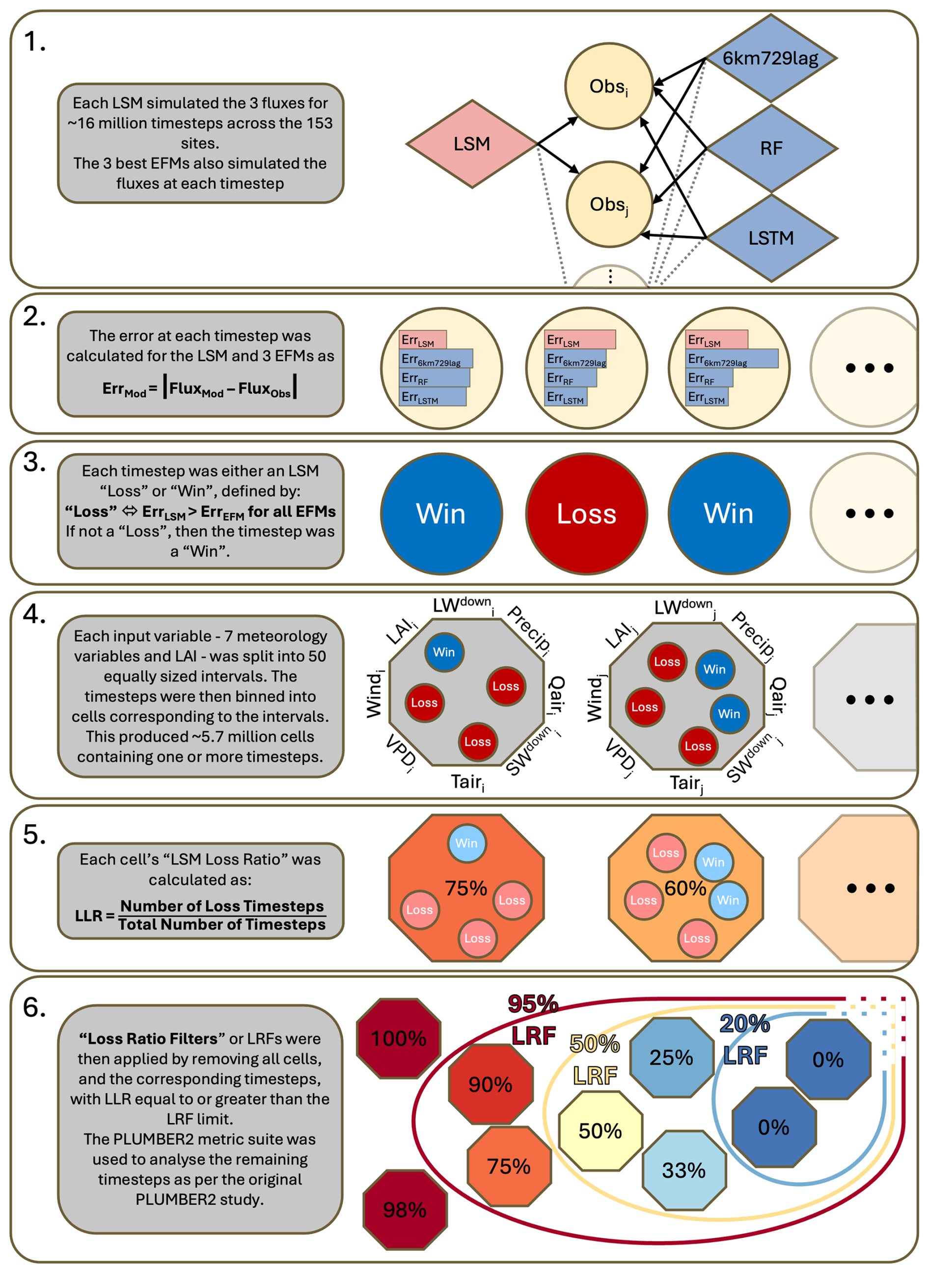
Figure 1 Schematic of Analysis Process. Circles indicate a timestep and octagons indicate a cell containing all timesteps that fall within a specific interval for each meteorological variable. The ellipses indicate that many other timesteps and cells are included in the full analysis.

If a timestep was not an LSM Loss, then we defined it as an “LSM Win” such that each timestep had a binary classification of whether or not we could expect the LSM to perform better under the corresponding conditions (step 3, Fig. 1). This definition was chosen to favour the LSMs. If the absolute LSM error was smaller than the absolute error of any of the best EFMs – that is, if the LSM outperformed just one of the three EFMs – we did not count this towards the definition of poor LSM performance. As previously mentioned, this reduced the influence of individual EFM model structure, meaning that poor LSM performance is more likely due to a general underutilisation of the information available in the input variables by the LSM. This in turn aimed to ensure that any areas of the input domain that exhibit poor performance under this definition are more likely to yield performance improvements if targeted for development. To illustrate the impact of such a definition of LSM Loss, consider the situation where an LSM and the best EFMs had equal performance across the entire domain of site-timesteps so that the differences between the four models were simply noise. We'd then expect a ratio of LSM Loss to LSM Win of 1:3. In other words, 25 % of timesteps would be an LSM Loss.

To explore the conditions under which the LSMs perform better or worse, we binned the input space based on eight input variables from the data measured at each site – SWdown, LWdown, Tair, Qair, VPD, Precip, Wind, and LAI. Each variable's range was split into fifty equally-spaced bins. With eight variables and fifty bins each, the input space was then split into 4×10¹³ unique cells across the 8-dimensional domain. Each cell was defined by the small sub-range of each of the eight input variables it contained. However, due to site distribution and the nature of meteorology, many of these cells were empty and some contained many more timesteps than others. For instance, cells corresponding to low SWdown values contained many timesteps due to roughly half of all the observational timesteps occurring at nighttime. Meanwhile, the PLUMBER2 dataset contains fewer sites that experience the extremes of temperature compared to temperate locations. Therefore, due to natural conditions and physically-determined interactions, the number of populated cells (i.e. cells with at least one timestep assigned to them) was far fewer than the total number of cells at slightly under six million (step 4, Fig. 1). The “LSM Loss Ratio” or LLR was then defined for each input cell as the percentage of timesteps in the cell that were an LSM Loss (step 5, Fig. 1). Hence, the LLR took a range of 0 % (the LSM outperformed at least one of the three best EFMs for every timestep in the cell) to 100 % (every timestep saw the LSM perform worse than all three of the best EFMs). The LLR provided a metric for LSM performance relative to the EFMs, and indicates the degree to which the LSMs are able to match the EFM's lower bound estimate of flux predictability for the small domain space contained within each cell. Cells with high LLR represent meteorological conditions under which the LSM(s) could be expected to perform better. In contrast, low LLR indicates meteorological conditions where our process understanding, LSM structure, and parametrisation are effective at utilising the available information to predict terrestrial fluxes. As noted above, if the LSM and best EFMs are equally capable, such that differences in their errors are random, then the LLR would be 25 %. Therefore, a LLR of 25 % or less indicates conditions where LSMs are reliably adding value.

We enabled visualisation of the results by collapsing the eight-dimensional input space into two-dimensional “fingerprints” via grouping the cells based on only two input variables at a time. We present plots of these fingerprints with Tair as one dimension and the other variables as the second dimension in turn. Tair was chosen as the constant x axis because it is intuitively easy to understand, has clear relationships with other meteorological variables, and its domain space is relatively uniformly represented by the site-timesteps, as opposed to the zero-dominated shortwave radiation for instance. Thus, we have two-dimensional fingerprints consisting of cells for which we calculated the LLR. We do not present the fingerprints for Qair because Qair and VPD are highly coupled.

2.2.2 Quantifying Impacts of Poor LSM Performance

While high LLR implies that the LSM(s) are underperforming compared to the EFMs, it does not quantify the magnitude of this underperformance. To do this, we utilised the metric suite from PLUMBER2 (Abramowitz et al., 2024). This consists of seven independent metrics (here meaning that any timeseries can be modified such that any one metric changes while the others remain constant), namely Mean Bias Error, Standard Deviation Difference, Correlation Coefficient, Normalised Mean Error, 5th Percentile Difference, 95th Percentile Difference, and Density Overlap Percentage. These capture information about the averages, distributions, and extremes of the timeseries as well as temporal correlation. Note that these were calculated on a site-by-site basis. To summarise these seven metrics, we utilised the independent normalised metric value (iNMV), introduced by PLUMBER2 and again calculated on a site-by-site basis. For metrics where lower values are better, the metric iNMV^m was defined as:

$$\begin{array}{}\text{(3)}& {\displaystyle }{\displaystyle }{\mathit{iNMV}}_{\text{LSM}}^m={\displaystyle \frac{m_{\text{LSM}}-min\left(m_{\text{benchmarkEFMs}}\right)}{max\left(m_{\text{benchmarkEFMs}}\right)-min\left(m_{\text{benchmarkEFMs}}\right)}}\end{array}$$

while for metrics where higher values are better, it was:

$$\begin{array}{}\text{(4)}& {\displaystyle }{\displaystyle }{\mathit{iNMV}}_{\text{LSM}}^m={\displaystyle \frac{max\left(m_{\text{benchmarkEFMs}}\right)-m_{\text{LSM}}}{max\left(m_{\text{benchmarkEFMs}}\right)-min\left(m_{\text{benchmarkEFMs}}\right)}}\end{array}$$

where m is the metric value, and the set of benchmark EFMs is as listed above. A lower iNMV^m is better. The mean iNMV^m across metrics and sites, iNMV, then provides a single number that synthesises LSM performance relative to EFMs. Since each of the seven metrics is weighted equally within this summary metric, the iNMV should adequately account for performance related to averages, extremes, and the distribution of the modelled timeseries as far as any aggregated metric can.

To assess the impact of poor LSM performance under the LSMs' worst meteorological conditions against other potential sources of poor LSM performance, we filtered the site-timesteps in five ways and compared the iNMV to the iNMV of the unfiltered data. Three of these filters were related to physical conditions, and two were “Loss Ratio Filters” (LRFs), where all timesteps that belong to input cells with a LLR above the threshold value were removed from the analysis, and performance impact of removing them was assessed (Fig. 1). Importantly, the LRFs were applied on the eight-dimensional input cells, not the two-dimensional fingerprints. The five filters were:

• A LRF of 95 %. All timesteps belonging to input cells with a LLR of 95 % or above were removed. This captured all conditions where the LSM was nearly always outperformed by the best EFMs.

• A LRF of 50 %. All timesteps belonging to input cells with a LLR of 50 % or above were removed. This provided an analysis that included only cells where the number of LSM wins outnumbered LSM losses. Due to the preference shown to the LSMs in the definition of an LSM Loss, this LRF significantly weighted the analysis towards conditions where the LSMs perform well compared to the best EFMs.

• A “Physical” consistency filter. This filter removed timesteps that consisted of physically impossible meteorological conditions. This involved calculating the saturated vapour pressure (SVP) at the observed air temperature and then removing any timesteps with a Qair or VPD value that violated this SVP. Such timesteps may occur due to observational error and could result in empirical models having an advantage where LSMs have strict constraints.

• A “Daytime” filter. All timesteps with SWdown less than or equal to 10 W m⁻² were removed. The assumptions underlying the eddy-covariance method can be violated at night-time (for instance, due to increased instances of insufficient turbulence), and hence night-time data can be heavily gap-filled (Aubinet et al., 2010, 2012; Pastorello et al., 2020).

• A “Windy” filter. All timesteps with Wind less than or equal to 2 m s⁻¹ were removed. This again was to account for potential measurements at times of insufficient turbulence. Wind speed was chosen over the friction velocity u^* to maintain consistency across the PLUMBER2 studies, with the wind speed threshold also being used in Abramowitz et al. (2024).

By applying these filters, we could gain an understanding of the areas of weak performance of LSMs, whether this was at night, being fed physically inconsistent inputs, or under particular meteorological conditions.

3 Results

Figure 2 shows the sensible heat flux LSM Loss Ratio (LLR) for the LSMs. Yellow indicates the null expectation of LSM performance (an LLR of around 25 %) where the LSM performed similarly to the best EFMs. This progresses to oranges and reds as LSM performance decreased and LLR increased. In contrast, LLRs of less than 20 % are coloured blue-green and indicate conditions where the LSMs were providing additional performance over the EFMs. The first column is an aggregated measure of LLR across all the LSMs using the root mean square of the individual LLRs. The Timesteps column shows the density distribution of the full dataset. Interestingly, across all potential input variable pairings with Tair, the largest LLRs for the root mean square (RMS) of all LSMs were seen in the edge cases – that is, located around the edge of the fingerprints. High LLRs occurred over the widest range of conditions when considering the LWdown-Tair interaction, with VPD-Tair and Wind-Tair also having more substantial areas of low LSM performance. There were no large discrepancies between the individual LSMs at LLRs above 80 % (light and dark red), with the “fingerprints” exhibiting similar patterns for poor LSM performance across models, and this is reflected too in the RMS fingerprints in the first column. At a LLR of 50 % or more (i.e. the LSM performing poorly at least half the time), differences between LSMs were clearer. For the VPD-Tair interaction, CABLE-POP had a high LLR across all conditions, while CABLE and both JULES implementations did worse at high VPD for the corresponding Tair (high LLR in the top right of the VPD-Tair domain). GFDL exhibited an inverse result with worse performance at low VPD-Tair values. The ORCHIDEE LSMs had a LLR of 50 % or more at VPD values with high but not extreme temperatures as seen from the dark orange streak to the right of the fingerprint, with surrounding lighter areas at higher temperatures. CHTESSEL_1, CLM5, and NoahMP had poor performance only at the boundaries of the Tair-VPD input space.

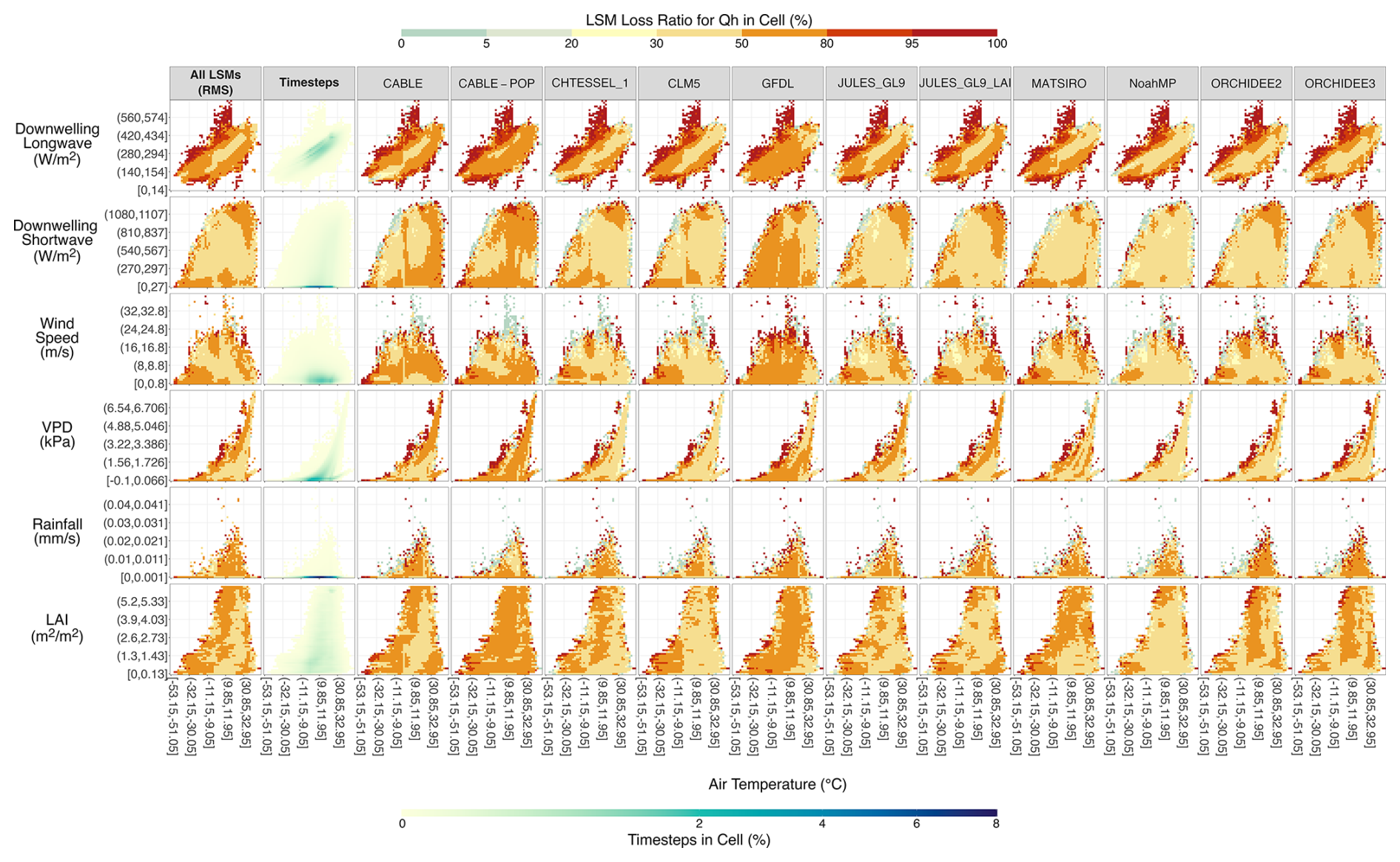
Figure 2 LSM Loss Ratio by Driving Variable and Model for Predicting Sensible Heat Flux. The x axis of each plot is air temperature and the y axis the other variables, each split into 50 equal-sized bins of which only every 10th bin is labeled. For the columns of individual models, each cell is coloured by the LSM Loss Ratio, the percentage of timesteps within the corresponding 2-D variable cell that are classified as an LSM Loss for the Qh flux. An LSM Loss of 0 occurs where, for every timestep within the cell, the LSM's absolute flux error is smaller than at least one of the absolute flux errors of the three best EFMs. Conversely, an LSM Loss of 100 occurs when the LSM's absolute flux error is greater than all three absolute flux errors of the best EFMs for all timesteps in the cell. For the timesteps column, the colour indicates the percentage of the total number of timesteps that fell within the 2-D variable cell. The “All LSMs” column is coloured by the root mean square of the LSM Loss across all models. Note that since all models simulated the same site-timesteps, the cells and timesteps within each cell are approximately the same but not equal for every model (some LSMs did not submit simulations for every site, missing four sites at most).

Figure 3 shows the Tair interaction LLR fingerprints for latent heat flux. While Qle had lower LLR values than Qh in general, it is still the case that the majority of high LLRs occurred in the edges of the fingerprints. However, in comparison to Qh (Fig. 2), it is not the case that most edge cells had poor LLR. In fact, many edge condition cells had LLR as low as 20 % or less. This indicates that, while LSMs still had areas of poor performance under edge conditions, there were also edge conditions under which Qle was well simulated relative to the EFMs. Hence, there were edge conditions where the LSMs have poor performance for Qh but good performance for Qle (for instance, compare the LWdown – Tair fingerprints in Figs. 2 and 3 where dark red areas in Fig. 2 are blue in Fig. 3). In turn, there were also edge conditions where both fluxes showed poor performance compared to the EFMs, such as can be seen in the VPD – Tair fingerprints. Particularly high LLR and poor LSM performance for Qle was seen at high VPD values relative to the concurrent Tair observation. Generally, as seen in the RMS of LLR for all LSMs and across most models independently, poor LSM performance for Qle did not appear to be dependent on LAI values, with the edge LLR rarely exceeding even 80 %, and the rest of the fingerprints' areas at 50 % or below.

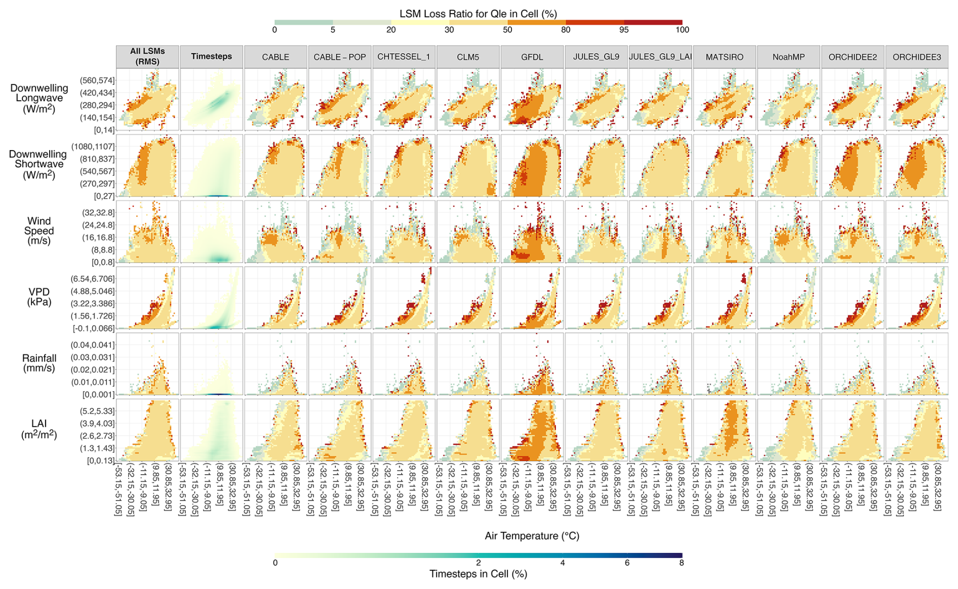
Figure 3 LSM Loss Ratio by Driving Variable and Model for Predicting Latent Heat Flux. The details are the same as Fig. 2 but for predictions of the Qle flux.

At low Tair (−30 °C or less), LLR was sub-20 % irrespective of input interactions across all LSMs, seen from the blue regions in columns 2 onwards in Fig. 3. For Qle, GFDL stands out as having the most potential for improvement in flux simulations. Extensive high LLR areas exist for all input condition interactions. GFDL has a LLR of around 20 %–50 % at high but not extreme temperatures indicating capacity for satisfactory simulation, yet performance began to decline around 10 °C. Other behaviours of note are the ORCHIDEE models having a similar drop in performance around a Tair value of 10 °C, although here the effect was moderated by interaction with other input conditions. The performance decline was seen only at the high/low LWdown boundaries, for SWdown values above ∼300 W m⁻², and for high VPD values. MATSIRO had high LLR (and hence poor relative performance) at Tair values around 0 °C when LAI is above ∼1 m² m⁻² but performed well at higher and lower temperatures.

Figure 4 completes the fingerprinting with the results for NEE. The LSM performance under edge conditions was much improved for NEE compared to the energy fluxes. In fact, there are substantial areas in Fig. 4 where the LSMs were providing additional value above the EFM simulations, often around the edge of the fingerprints. High LLRs still occurred at the boundaries of the Tair-VPD and Tair-Wind fingerprints yet were interspersed with cells of good LSM performance. However, inter-LSM differences were conspicuous for the carbon flux. NoahMP struggled against the EFMs relative to the rest of the LSMs: there was a pronounced temperature effect with a gradient of generally increasing LLR as Tair values increased. This dominant role of Tair appeared, but with a more subtle impact, for the other LSMs to varying degrees with greater regions of worse LLR (orange and red tones) towards higher temperatures and good performance (blue tones) towards lower temperatures. CABLE and CHTESSEL_1 were the other two LSMs that exhibited LLRs of 50 % or more at higher temperatures, while the two ORCHIDEE models in particular have only small regions of high LLR.

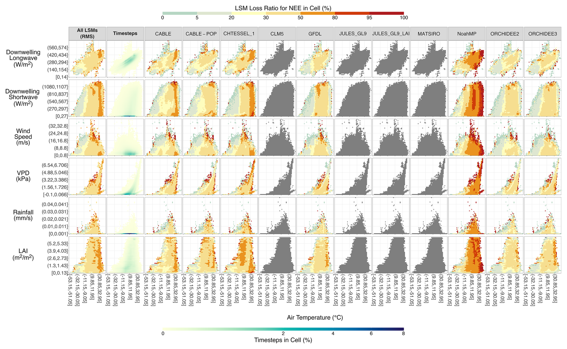
Figure 4 LSM Loss Ratio by Driving Variable and Model for Predicting Net Ecosystem Exchange. The details are the same as Fig. 2 but for predictions of the NEE flux. Note that greyed out LSMs did not provide half-hourly NEE outputs to the PLUMBER2 experiment.

Figure 5 shows the independent normalised metric values (iNMV) for each LSM defined by the range of metric values of the three benchmark EFMs. This is a measure of LSM performance based on the benchmark EFM performance, directly comparable across LSMs (note the differing y axes). The grey lines indicate the 3 PLUMBER2 benchmark EFMs – 1lin, 3km27, and LSTM – with different symbols to differentiate between the EFMs and darker greys as the complexity increases. The black line is the base LSM performance. The blue lines are the LSM results when filters were applied, either using only daytime timesteps (dark blue), timesteps with sufficient wind (mid blue), or timesteps that did not violate physical humidity limits (light blue). The orange (95 %) and red lines (50 %) are the LSM results when timesteps are filtered based on the LSM Loss Ratio. In all cases, iNMV was calculated using the benchmark metrics as calculated on the original dataset i.e. no filters were ever applied to the benchmark models – their iNMV values are always calculated on the entire dataset. The black lines indicate the raw LSM performance as in the PLUMBER2 benchmarking framework and are therefore almost exactly the same result as Abramowitz et al. (2024) (there are slight differences due to using one less site here). As per Abramowitz et al. (2024), LSMs mostly performed worse than the benchmark EFMs, with all 11 LSMs performing worse than a simple linear model for simulating Qh. Better performance was seen in the other two fluxes, with most LSMs' performance falling between the linear model and the “3km27” k-means clustering model for Qle. For NEE, three of the seven LSMs in this analysis beat the linear model performance.

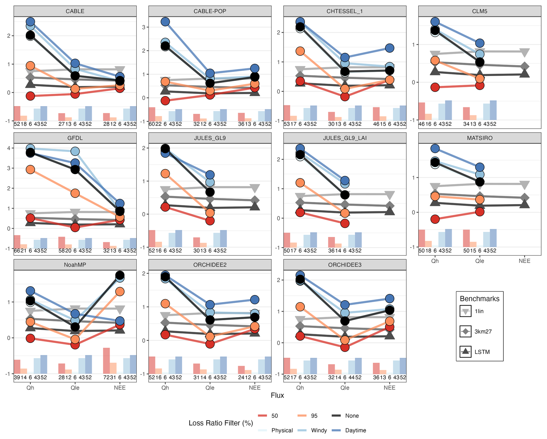
Figure 5 LSM Performance after Application of Different Timestep Filters. The three fluxes are on the x axis, and the y axis is the independent normalised metric value iNMV. Note that the y axis varies for each facet. Each facet is for an individual LSM. Lower iNMV is better. The grey lines are the benchmark EFMs, the black line is the original LSM, and the blue and red lines are the LSM under different filters including the 95 % and 50 % Loss Ratio Filters as well as Daytime, Windy, and Physical filters. The bar charts and labels indicate the percentage of timesteps removed by each of the five filters. Note the differing y axis scales and that the “Physical” filter is often obscured by the “None” LRF/original model performance.

The iNMVs for two different LRFs are also shown in Fig. 5. The first, a LRF of 95 %, indicates the LSM performance when timesteps in poorly modelled input cells were removed from the analysis. These are the darker cells from Figs. 2–4. The percentage of timesteps removed by this filter varied from 12 % (CABLE and ORCHIDEE2 for NEE, CABLE-POP and NoahMP for Qle) to 31 % (also NoahMP but for NEE). The mean percentage of timesteps removed by the 95 % LRF was 17 % for Qh, 14 % for Qle, and 16 % for NEE. The 95 % LRF substantially improved iNMV for many of the models for all three fluxes (indicated by the difference between the black “None” and orange “95” points). The mean relative improvement in iNMV across all fluxes and models was 56 % (Table S1 in the Supplement). Noteworthy cases include many models (CABLE, CHTESSEL_1, CLM5, JULES_GL9, and the ORCHIDEE LSMs) improving from beating only the “1lin” model to being better than even the “LSTM” when simulating Qle (the mean relative improvement of iNMV for Qle under the 95 % LRF was 77 %). The Qh simulations from CABLE-POP, CLM5, MATSIRO, and NoahMP improved from a drastically worse performance than any of the EFM benchmarks to at least beating the “1lin” model (iNMV improvements of 69 %, 58 %, 68 %, and 57 % respectively). The impact of the 95 % LRF was less substantial for the NEE flux with smaller improvements across the LSM suite (mean iNMV relative improvement of 36 %).

The 50 % LRF was a drastic filter application. Any timesteps located in input cells with a LLR of 50 % or higher were removed from the metric calculations. This means that theoretically, within any single removed input cell, there were still up to 50 % of the removed timesteps that were instances where the LSMs actually beat (at least one of) the best EFMs. The largest improvement here was seen in the Qh flux simulations, where all LSMs but CHTESSEL_1 and GFDL beat the “LSTM” model under the 50 % LRF (mean relative iNMV improvement of 97 %, Table S2 in the Supplement). Differences between the 50 % and 95 % LRFs were minimal for Qle and NEE. The exception was Qle from GFDL where at the 95 % LRF, GFDL was still outperformed by the “1lin” EFM but at the 50 % LRF, GFDL can beat the “LSTM” EFM. Necessarily, the 50 % LRF resulted in the exclusion of a greater percentage of timesteps. Individual LSMs range from 24 % to 72 % (ORCHIDEE2 and NoahMP respectively, both for NEE) of timesteps removed. A mean of 52 % of timesteps were removed for the Qh flux, 35 % for Qle, and 39 % for NEE.

As clear in Figs. 2–4, the original PLUMBER2 dataset includes timesteps that represent physically-impossible conditions. For instance, there are timesteps that fall outside of the VPD-temperature curve which is well-defined by the laws of thermodynamics. Such instances could be due to observational error, poor gap-filling, or incorrectly applied quality control. These timesteps have been retained in the LRF filters in this analysis as they feature in the published PLUMBER2 dataset. However, we also plotted the iNMV of the LSMs when the physically inconsistent timesteps were removed (the “Physical” LRF in light blue). The performance for most models and fluxes was almost indistinguishable from the raw LSM performance (mean relative iNMV improvement of 1 % across all fluxes, Table S3 in the Supplement) and only 6 % of timesteps were removed.

Another non-LRF filter is the “Daytime” filter, implemented by removing all timesteps with a SWdown value of 10 W m⁻² or less. This removed 52 % of the timesteps in the base analysis, a substantial amount. However, in nearly all cases, the LSM performance for Qh was degraded by applying this filter (Table S4 in the Supplement), with higher iNMV for all LSMs except GFDL and JULES_GL9 (relative iNMV improvement of 1 % and 7 % respectively). For Qle, the LSM performance was always worse for the Daytime filter. In fact, for many LSMs, the base performance beat the “1lin” benchmark while the Daytime filter resulted in even this simple EFM performing better than the LSM. The relative difference in iNMV varied from −11 % (GFDL) to −120 % for NoahMP. The Daytime filter also resulted in worse NEE performance for all LSMs except NoahMP which struggled with simulating NEE under the original conditions (Fig. 4). NoahMP saw a dramatic performance increase (73 % relative iNMV improvement) from failing to beat the “1lin” benchmark to nearly matching the “3km27” benchmark. Significant declines in performance (i.e. a negative change in the EFM benchmark beaten) were seen for CHTESSEL_1 (−108 % iNMV relative difference) and ORCHIDEE2 (−76 % iNMV change) simulations of NEE in terms of EFM benchmark thresholds (from beating “1lin” to not).

The final filter is a “Windy” filter where timesteps with a wind speed of 2 m s⁻¹ or less were removed from the iNMV calculations for the LSMs. With the intention of removing timesteps of insufficent turbulence for effective eddy-covariance measurements, the iNMV under this filter was generally degraded (Table S5 in the Supplement), falling between the original LSM iNMV and the Daytime NMV. This filter removed 43 % of timesteps. Performance was degraded for Qle (mean relative iNMV difference of −39 %) while Qh and NEE saw little change (mean relative iNMV differences of −4 % and −5 % respectively).

4 Discussion

LSMs are under constant cycles of development with multiple modelling teams across the globe dedicated to improving their performance. By benchmarking LSMs against three different out-of-sample EFMs that performed well when predicting site fluxes, we provide insight for model development and assessment. This was not a “beauty contest” between LSMs – comparing LSMs directly against each other fails to account, for example, for instances where all models are underperforming. Similarly, direct comparison to observations fails to account for the level of inherent predictability in flux measurements (Haughton et al., 2018a, b; Di et al., 2023). Importantly, we also do not address here the absolute performance of the LSMs. Instances of poor LSM performance, as defined in this study, may in fact occur where both LSMs and EFMs are performing objectively well compared to the observations. On the converse, we may here report good LSM performance where the LSMs and EFMs have significant absolute errors compared to observations. Instead, by considering performance relative to out-of-sample EFMs, we can infer a lower bound estimate of predictability that LSMs theoretically should be capable of achieving (Nearing et al., 2018).

Importantly, all EFMs simulations were produced out-of-sample on a site-by-site basis, meaning that they were not exposed to any information from the site they were tasked with simulating. This increases the information provided by the benchmark of prediction skill. For instance, suppose there exists a process that LSMs are assumed to struggle to represent accurately, for example, the temperature acclimation of photosynthesis (Oliver et al., 2022; Ren et al., 2025). If the EFMs also struggle under these conditions, then LSM development may be ill-spent focused on improving the representation of this process because the poor EFM performance would indicate that we lack the necessary information (whether missing observations of related processes or even the processes themselves) to easily improve LSM performance. Instead, in areas where the EFMs outperform the LSMs by a substantial margin, we can hypothesise that we have the information required to model the process accurately. In such areas, targeted LSM development may see easier performance gains.

In line with this, our results show that model improvements targeted to behaviour in a small number of specific meteorological conditions could significantly improve LSM performance. For instance, consider the MATSIRO LSM simulations of sensible heat. As illustrated in Fig. 5, in the PLUMBER2 analysis across all site-timesteps, MATSIRO underperformed with simulations worse than a simple linear regression. However, when we applied the 95 % LRF, the performance of MATSIRO dramatically improved. Removing 17 % of timesteps resulted in MATSIRO leapfrogging the “1lin” model and even beating the “3km27” benchmark. Figure 2 shows where these 17 % of timesteps are located in meteorological space – conditions of high VPD and high wind speed relative to air temperature as well as high and low temperature values relative to incoming longwave radiation. That is, removing a small number of timesteps located in discrete meteorological conditions resulted in a substantial performance improvement. This was especially true for sensible heat flux where the message of the PLUMBER2 analysis (Abramowitz et al., 2024) – that for sensible heat simulations, LSMs were consistently beaten by a simple linear model – would significantly change. The LSM simulations of Qle improved dramatically under the 95 % LRF, frequently improving the EFM benchmark threshold they could beat to the best EFM in the analysis. This implies that, compared to the other two fluxes, the performance of the LSM in predicting Qle was dominated by a few poorly modelled instances. In other words, there were timesteps (less than 20 % for all models, see dark red cells in Fig. 3) where the LSM performance was so much worse than the average performance that these outliers significantly skewed the metrics towards worse performance.

An interesting result is that the only substantial improvement in model performance when applying the “Daytime” filter is for the NEE flux simulated by NoahMP. For all other models, the “Daytime” LRF reduces NEE performance. This would suggest that the poor performance of NoahMP for NEE is related to soil respiration which dominates nighttime fluxes. The lack of similar improvement in the “Windy” filter applied to NoahMP supports this. Similarly, the other LSMs having worse NEE performance when filtering out nighttime timesteps would indicate that these LSMs more accurately capture the soil respiration. This might in turn mean that the other LSMs are not as competent in simulating GPP as the original PLUMBER2 results for NEE suggest. Of course, such inferences might be tempered by the possible poor nighttime flux data meaning that the LSMs are attempting to simulate biased data at nighttime.

Figures 2–4 visualise the LSM input space through two-dimensional fingerprints in combinations of input variables interacting with Tair. There was a clear “edge effect” for all three fluxes, albeit of varying magnitude. This indicates that LSM performance was weak whenever an extreme value in the input space of a variable coincided with an extreme air temperature relative to the variable value in question. In other words, the edge effect was itself two-dimensional. For example, the LSM performance for sensible heat was notably weaker at the edge values of longwave radiation and air temperature. These edge conditions would imply extreme levels of humidity and/or cloudiness (the drivers of longwave radiation) compared to the temperature. The weaker LSM performance at these timesteps may relate to site water availability and the LSMs incorrectly partitioning energy between sensible and latent heat, poor representation of the effects of direct vs diffuse radiation, or perhaps even changes in the heat capacity of the air that are not considered within the LSMs. Another notable edge effect is seen in the VPD-Tair fingerprints where LSMs have high LSM Loss Ratios for both sensible and latent heat in the upper edge cells (Figs. 2 and 3). This implies that at times of relatively high VPD and low humidity for the given temperature, LSMs struggle to predict Qh and Qle well relative to the EFMs. This could potentially arise from incorrect energy partitioning in the LSMs (Yuan et al., 2022). Similar high LLRs are seen at high relative VPD for NEE (Fig. 4) but to a lesser extent, with cells at the lower and upper ends of the temperature range exhibiting good performance for the carbon flux. Interestingly, NEE performance also suffers under high relative temperatures for a given VPD. This may be further evidence for the energy partitioning explanation since the LSMs can perform well for NEE in some of the same regions that they struggle for Qh and Qle. This would align with Haughton et al. (2016) who found that, in the original PLUMBER analysis, LSM errors were largely attributable to energy partitioning within the LSMs. Yet another edge case is at high wind speeds, relative to Tair, where substantial LSM losses occur for all three fluxes. Future work should investigate which of these possible causes may be responsible for the specific edge effects.

Figure 4 indicates that a relationship between temperature and LSM performance appears to exist for NEE. For NoahMP in particular, and CABLE and CHTESSEL_1 to a lesser degree, there is a clear progression from low LLR to high LLR as air temperature increases. This relationship also exists for CABLE-POP, GFDL, ORCHIDEE2, and ORCHIDEE3 but with generally better LSM performance. One potential reason for better LSM performance at low temperatures is simply that photosynthesis and repsiration are significantly diminished or zero at cold temperatures which is easy to incorporate in LSMs through temperature thresholds. Another potential cause could be the temperature acclimation of photosynthesis at higher temperatures with LSMs struggling to model this process (Blyth et al., 2021; Mengoli et al., 2022). Interestingly, all LSMs except NoahMP still exhibit an edge effect at higher temperatures with the most extreme high temperatures also showing good LSM performance.

LSMs are often tested against certain types of climatic extreme events as part of their development. For instance, LSM performance under drought conditions (De Kauwe et al., 2015; Ukkola et al., 2016; Huang et al., 2016; Harper et al., 2021) and heatwaves (Mu et al., 2021a, b) is heavily studied. It is worth noting that while these extremes operate at longer timescales than the half-hourly data explored here, they necessarily need to result from processes simulated at the half-hourly timescale in these models. When data is temporally aggregated from this half-hourly timestep – even to the 6-hourly inputs of e.g. TRENDY (Sitch et al., 2024) – the extreme edge cases are averaged out. However, it is likely more difficult for LSMs to capture the high-resolution behaviour at the sub-daily scale than averages over longer periods. For example, it would be theoretically possible to simulate perfect monthly average fluxes and have poor, but compensating, process representations at the shorter timescales. In the extreme case, an LSM could even simulate the diurnal cycle out of phase by 12 h, and this may not be apparent when performance is analysed at monthly timescales. Interestingly, Haughton et al. (2016) showed that, for the original PLUMBER experiment, temporal aggregation made no significant difference to LSM performance relative to EFMs. This may indicate that LSMs submitted to other benchmarking and comparison studies are too heavily calibrated to the aggregated data on which they are applied. Our results indicate that LSM behaviour under all types of short-term climatic extremes is worthy of investigation, including during colder temperatures and varying humidity levels. This edge effect is then most likely explained by the parametrisation of LSMs not being tested on meteorological edge conditions at high temporal resolution to the degree necessary. A potential reason for this lack of parametrisation testing at the input boundaries is the complexity of the LSMs. The number of parameters in LSMs is increasing over time (Fisher and Koven, 2020) as development attempts to improve the representation of numerous model components, such as soil structure and hydrology (Fatichi et al., 2020; Xu et al., 2023). This increasing complexity may not be ideal given that most parameters are poorly constrained (Shiklomanov et al., 2020; Famiglietti et al., 2021).

Interestingly, by their nature and as illustrated in the fingerprints of Figs. 2–4, these edge cells contained fewer timesteps than the cells near the centre of the variable distribution. As such, there was much less training information available for these conditions for the EFMs – in fact, these edge cells were often populated with timesteps entirely from a single site (see Fig. S1 in the Supplement). Since the EFMs were trained out-of-sample, they potentially had zero training data from these extreme conditions. As such, it might be assumed that EFM performance would be at its worst at the edge. Yet it was within these data-sparse regions that the EFMs outperformed the LSMs. This would imply that the flux behaviour under the extreme conditions can be learned from other areas of the input space. Hence, it is unlikely to be novel processes or missing biophysical interactions that limit LSM performance in this space. In fact, Haughton et al. (2016) found in the first PLUMBER experiment that, on a site-by-site basis, LSMs could perform much better than EFMs at unique sites dominated by less-common behaviour or unusual processes. Another consideration is the temporal nature of these edge timesteps – did the extremes come from consecutive timesteps during an extreme event or do they occur only as random noise in the measurements? While we did not explicitly assess the temporal connections within our framework, if these coinciding extreme values did occur only due to random noise, then we might expect the EFMs to perform worse than the LSMs here. Since most of the extreme values are observed at single sites (Fig. S1), the EFMs have no visibility of data from the exact same conditions when simulating the timestep and should therefore equally struggle to accurately model random noise. A next step here may be exploring the results at site-level to identify more explicitly the processes in action within each cell with a high LLR.

Figures S2–S4 in the Supplement show the LSM fingerprints for the mean LSM error relative to the observations within each cell for Qh, Qle, and NEE respectively. While not considered in-depth in the same manner as the benchmarking, a few key findings stand out. Firstly, the magnitude of mean error exhibits a similar edge effect to the benchmarking losses with larger mean errors towards the edges of the two-dimensional. As such, targeting model developments at these cells is not only feasible as shown by the benchmarking results in Figs. 2–4 but also targets the objectively worst performing conditions when considered against observations. Evidence for the power of our benchmarking and LSM Loss framework is evinced by the LSMs' mean error for NEE, especially NoahMP (Fig. S4). While the mean error tends to have a greater magnitude at higher temperatures as most evident for NoahMP, the clear relationship between temperature and LSM performance (in terms of the LLR) with higher temperatures having higher LSM Loss Ratios (Fig. 4) is not discernible. In general, high LLR does not align with consistent under- or overestimation. A good example is GFDL's performance for latent heat (Figs. 3 and S3). A large area of high LLR at mid to low temperatures contains cells with positive and negative mean errors. Since no clear relationship exists between areas of high LLR and the LSM mean error, we recommend that model developers use LLR benchmarking to identify priority areas before assessing the model error and other metrics to pinpoint which processes or parameters may need additional consideration.

The importance of observations at particular meteorological extremes is clear from the edge effect observed here. Such analysis is only possible because the existing eddy-covariance networks have managed to capture these conditions. However, van der Horst et al. (2019) showed that the current network of flux towers undersamples high temperature conditions. It is likely also the case that the potential extremes of other variables are also underobserved. As such, there is a need for increased observations from ecosystems exposed to extreme meteorology (in this multi-dimensional sense). This is important both because of the performance edge effect we noted here, and the fact that these conditions will likely become more common than they have been historically. While additional flux towers are an easy and obvious request, two other actions could be taken. The first and simplest is ensuring that existing towers can operate during the extremes experienced at their locations by enhancing protection from the elements and disturbances. Secondly, the rapid deployment of portable flux measurements when meteorological extremes are forecast could help develop the necessary dataset of extreme observations. Such deployments could be eddy-covariance towers (Billesbach et al., 2004; Ocheltree and Loescher, 2007), leaf-canopy or footprint-scale (respiration chambers) measurement campaigns, that could complement ecosystem-scale understanding.

As mentioned for the Fig. 5 results, the PLUMBER2 analysis contains some timesteps that are physically inconsistent based on temperature and humidity relationships. It was possible that such timesteps may have negatively affected this analysis – the EFMs were not constrained by physics and so were more likely to be able to accurately model these timesteps than the LSMs. The manner in which individual LSMs handle physical inconsistency in inputs may also differ in methodology and therefore the impact on LSM performance. However, removing these timesteps from the analysis did not improve LSM performance, with any changes in iNMV minimal. Approximately 6 % of the timesteps were removed, representing a non-negligible portion of the data. Whether the ability of the LSMs to robustly deal with such physically-inconsistent inputs is reassuring (since model outputs did not massively degrade when forced by them) or of concern (why should we expect LSMs to be able to simulate fluxes under these unpredictable conditions?) is unclear and is an area for further research.

5 Conclusions

We have shown that the LSM underperformance relative to empirical benchmarks reported by the PLUMBER2 experiment can largely be attributed to LSM performance under specific conditions. In other words, LSMs perform significantly better and can beat better EFM benchmarks when certain meteorological conditions are excluded from the analysis. Notably, the conditions of markedly poor LSM performance occur in only a fraction of the total site-timesteps being considered with the majority occurring under coinciding extremes of two or more meteorological variables. In particular, the concurrent extremes, both low and high, of incoming longwave radiation and air temperature result in poor LSM performance for sensible heat. In addition, LSM performance under high values of VPD relative to air temperature show strong potential for improvement for all three fluxes of sensible heat, latent heat, and net ecosystem exchange. Hence, the timesteps of poor performance are mostly described by a edge effect visible in 2-dimensional fingerprints of meteorological input space. By focussing LSM development on the dominant processes at these half-hourly mutual extremes of multiple drivers, we have shown that substantial performance gains could be realised. This places clear value on observations of ecosystem fluxes at these meteorological edge conditions. Without observations of these conditions, the continued advancement of LSMs is constrained by a lack of calibration and testing data. Targeted field campaigns, using rapid deployments to sample responses, may be a necessary step to guide efficient future LSM development and process refinement.